Arctic Ocean CO₂ uptake: an improved multiyear estimate of the air–sea CO₂ flux incorporating chlorophyll a concentrations

We estimated monthly air–sea CO₂ fluxes in the Arctic Ocean and its adjacent seas north of 60^∘ N from 1997 to 2014. This was done by mapping partial pressure of CO₂ in the surface water (pCO_2w) using a self-organizing map (SOM) technique incorporating chlorophyll a concentration (Chl a), sea surface temperature, sea surface salinity, sea ice concentration, atmospheric CO₂ mixing ratio, and geographical position. We applied new algorithms for extracting Chl a from satellite remote sensing reflectance with close examination of uncertainty of the obtained Chl a values. The overall relationship between pCO_2w and Chl a was negative, whereas the relationship varied among seasons and regions. The addition of Chl a as a parameter in the SOM process enabled us to improve the estimate of pCO_2w, particularly via better representation of its decline in spring, which resulted from biologically mediated pCO_2w reduction. As a result of the inclusion of Chl a, the uncertainty in the CO₂ flux estimate was reduced, with a net annual Arctic Ocean CO₂ uptake of 180 ± 130 Tg C yr⁻¹. Seasonal to interannual variation in the CO₂ influx was also calculated.

1 Introduction

The Arctic Ocean and its adjacent seas (Fig. 1) generally act as a sink for atmospheric CO₂ because of the high solubility of CO₂ in their low-temperature waters, combined with extensive primary production during the summer season (Bates and Mathis, 2009). The Arctic Ocean and its adjacent seas consist of complicated subregions that include continental shelves, central basins, and sea-ice-covered areas. Therefore, the surface partial pressure of CO₂ (pCO_2w) distribution is not only affected by ocean heat loss and gain, and biological production and respiration, but also by sea ice formation and melting, river discharge, and shelf–basin interactions (see Bates and Mathis, 2009, and references therein). However, CO₂ measurements are sparse in this very heterogeneous area (Fig. 2), and hence the existing air–sea CO₂ flux estimates in the Arctic are poorly constrained (Bates and Mathis, 2009; Schuster et al., 2013; Yasanuka et al., 2016).

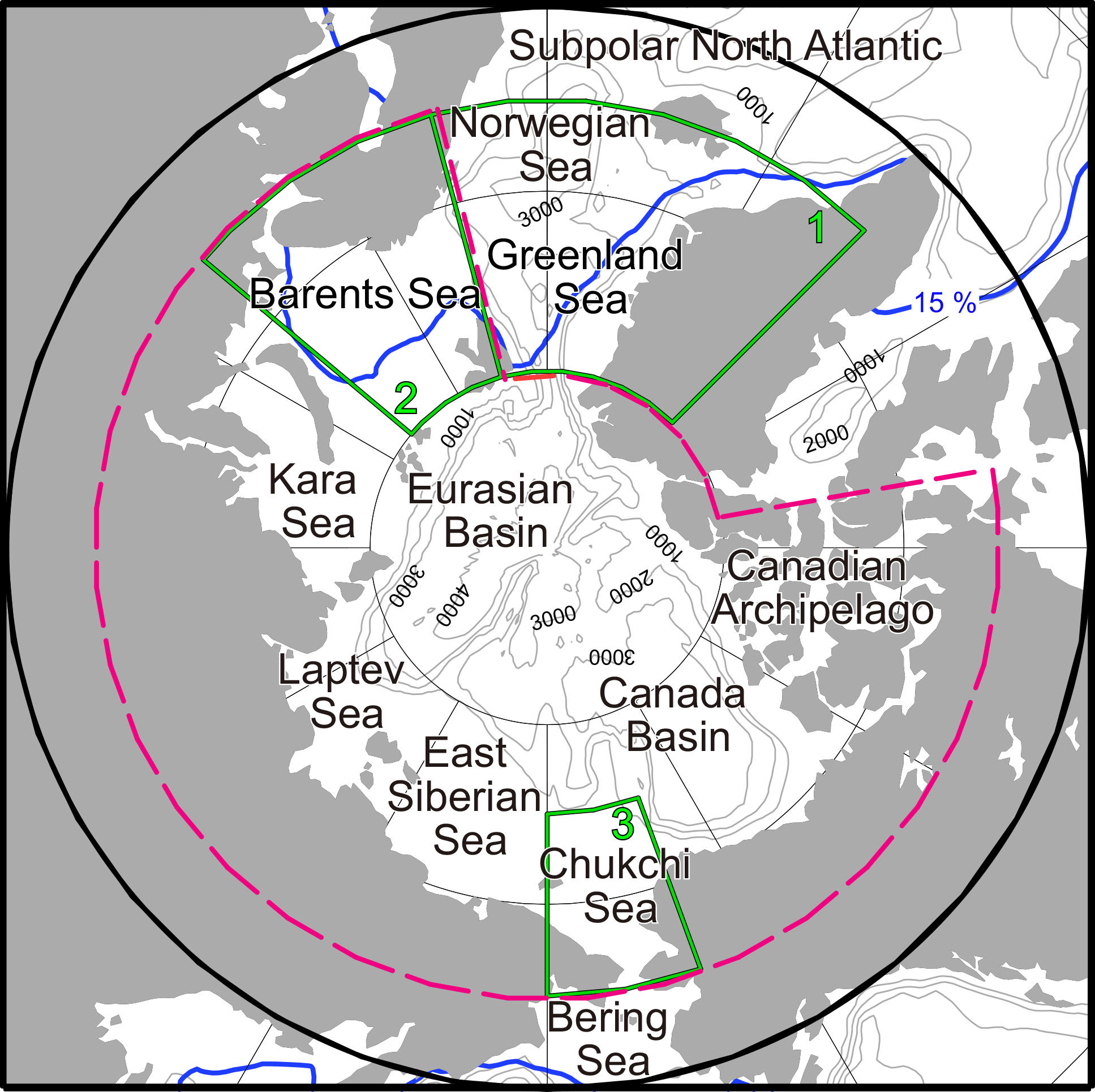
Figure 1 Map of the Arctic Ocean and its adjacent seas. Gray contour lines show the 1000, 2000, 3000, and 4000 m isobaths. Blue lines show the 17-year annual mean position of the ice edge (SIC = 15 %). Area for the mapping is north of 60^∘ N (heavy black circle). Sectors selected for regional analysis are the Arctic Ocean (dashed magenta line), the Greenland and Norwegian seas (green 1), the Barents Sea (green 2), and the Chukchi Sea (green 3).

As global warming progresses, melting of sea ice will increase the area of open water and enhance the potential for atmospheric CO₂ uptake (e.g., Bates et al., 2006; Gao et al., 2012). However, other processes could suppress CO₂ uptake. For example, increasing seawater temperatures, declining buffer capacity due to the freshening of Arctic surface water by increased river runoff and melting of sea ice, and increased vertical mixing supplying high-CO₂ water to the surface will all result in a tendency for reduced uptake (Bates and Mathis, 2009; Cai et al., 2010; Chierici et al., 2011; Else et al., 2013; Bates et al., 2014; Fransson et al., 2017). The combined effect of all these processes on ocean CO₂ uptake has not yet been clarified for the Arctic.

Yasunaka et al. (2016) prepared monthly maps of air–sea CO₂ fluxes from 1997 to 2013 for the Arctic north of 60^∘ N by applying, for the first time, a self-organizing map (SOM) technique to map pCO_2w in the Arctic Ocean. The advantage of the SOM technique is its ability to empirically determine relationships among variables without making any a priori assumptions (about what types of regression functions are applicable, and for which subregions the same regression function can be adopted, for example). The SOM technique has been shown to reproduce the distribution of pCO_2w from unevenly distributed observations better than multiple regression methods (Lefèvre et al., 2005; Telszewski et al., 2009). The uncertainty of the CO₂ flux estimated by Yasunaka et al. (2016), however, was large (± 3.4–4.6 $\mathrm{mmol}{\mathrm{m}}^{-\mathrm{2}}{\mathrm{d}}^{-\mathrm{1}}$), and the estimated CO₂ uptake in the Arctic Ocean was smaller than the uncertainty (180 ± 210 Tg C y⁻¹). One possible reason for the large uncertainties is that no direct proxies for the effect of biological processes on pCO_2w were used in that study, leading to an underestimation of the seasonal amplitude of pCO_2w.

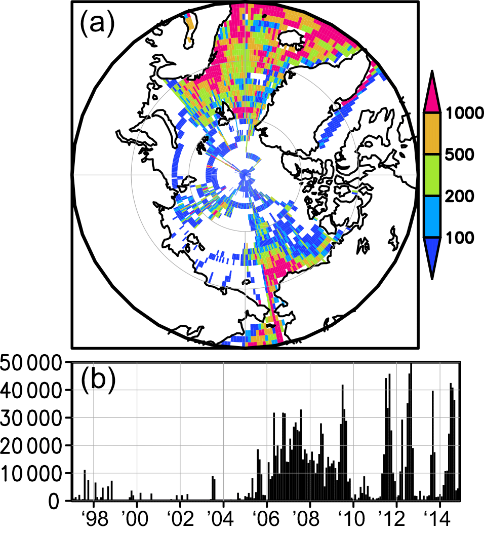
Figure 2 (a) The number of ocean surface CO₂ data in the grid boxes (1^∘ × 1^∘) used in this study. Data are from SOCATv4, LDEOv2014, and GLODAPv2 and those collected by R/V Mirai of JAMSTEC between 1997 and 2014. (b) Monthly number of CO₂ data in the analysis area (north of 60^∘ N) from 1997 to 2014.

Remotely sensed chlorophyll a concentrations (Chl a) have been used in several pCO_2w mapping efforts as a direct proxy for the effect of primary production. For example Chierici et al. (2009) produced pCO_2w algorithms for the subpolar North Atlantic during the period from May to October and found that the inclusion of Chl a improved the fit substantially. Measurements in several areas of the Arctic show that relationships between pCO_2w and Chl a also occur in this region. They correlate negatively (Gao et al., 2012; Ulfsbo et al., 2014), as expected from the drawdown of CO₂ during photosynthesis, but exceptions do occur; in coastal regions the correlation is positive (Mucci et al., 2010).

Several studies have demonstrated that Chl a in the Arctic can be estimated from satellite remote sensing reflectance (Rrs) (e.g., Arrigo and van Dijken, 2004; Cota et al., 2004). Perrette et al. (2011) showed that satellite-derived Chl a successfully captured a phytoplankton bloom in the ice edge region. Changes in the seasonal cycle from a single peak to a double peak of Chl a have also been detected and are likely a consequence of the recent sea ice loss in the Arctic (Ardyna et al., 2014). However, the available products (e.g., NASA's OceanColor dataset) in the Arctic include large uncertainty and many missing values because of sea ice, low angle of sunlight and cloud cover, and are also prone to error due to the co-occurrence of high colored dissolved organic matter (CDOM) and total suspended matter (TSM) concentrations (e.g., Matsuoka et al., 2007; Lewis et al., 2016). Here we deal with these issues by using several Chl a algorithms optimized for the Arctic and others, and by excluding Chl a data from grid cells potentially affected by CDOM and TSM. Calculated Chl a values were then interpolated so as to fit with the original data. Using these data, we examined the relationship between pCO_2w and Chl a in the Arctic Ocean and its adjacent seas and computed monthly air–sea CO₂ flux maps for regions north of 60^∘ N using a SOM technique similar to that of Yasunaka et al. (2016) and with Chl a added to the SOM process.

2 Data

2.1 pCO_2w measurements

We used fugacity of CO₂ (fCO_2w) observations from the Surface Ocean CO₂ Atlas version 4 (SOCATv4; Bakker et al., 2016; http://www.socat.info/; 1 983 799 data points from > 60^∘ N), and pCO_2w observations from the Global Surface pCO₂ Database version 2014 (LDEOv2014; Takahashi et al., 2015; http://cdiac.ornl.gov/oceans/LDEO_Underway_Database/; 302 150 data points from > 60^∘ N). In the LDEO database, pCO_2w is based on measured CO₂ mixing ratio in a parcel of air equilibrated with a seawater sample and computed assuming CO₂ as an ideal gas, whereas in the SOCAT, fCO₂ is obtained considering the non-ideality from CO₂–CO₂ and CO₂–H₂O molecular interactions. Because of ambiguities in the CO₂–H₂O interaction corrections, the SOCAT fCO_2w values are converted to pCO_2w values (a correction of < 1 %) and then combined with the LDEO pCO_2w values. When data points were duplicated in the SOCAT and LDEO datasets, the SOCAT version was used, except for the data obtained from onboard the USCGC Healy as these have been reanalyzed by Takahashi et al. (2015). Altogether 200 409 duplicates were removed. We also used shipboard pCO_2w data obtained during cruises of the R/V Mirai of the Japan Agency for Marine-Earth Science and Technology (JAMSTEC) that have not yet been included in SOCATv4 or LDEOv2014 (cruises MR09_03, MR10_05, MR12_E03, and MR13_06; available at http://www.godac.jamstec.go.jp/darwin/e; 95 725 data points from > 60^∘ N). In total, we used 2 181 265 pCO_2w data points, 33 % more than used by Yasunaka et al. (2016).

To further improve the data coverage, especially for the ice-covered regions, we also used 2166 pCO_2w values calculated from dissolved inorganic carbon (DIC) and total alkalinity (TA) data extracted from the Global Ocean Data Analysis Project version 2 (GLODAPv2; Key et al., 2015; Olsen et al., 2016; http://www.glodap.info). Of these data, 90 % were obtained at cruises without underway pCO_2w data. We extracted values of samples obtained from water depths shallower than 10 m, or the shallowest values from the upper 30 m of each cast if there were no values from above 10 m. There are 1795 data points above 10 m depth, 296 in the 10–20 m range, and 75 in the 20–30 m range. This resulted in 94 % more calculated pCO_2w values than used by Yasunaka et al. (2016), and altogether the number of directly measured and calculated data points used here is 33 % more than used in Yasunaka et al. (2016). The CO2SYS program (Lewis and Wallace, 1998; van Heuven et al., 2009) was used for the calculation with the dissociation constants reported by Lueker et al. (2000) and Dickson (1990).

We checked the difference between calculated pCO_2w and measured pCO_2w using the data from cruises with both bottle DIC and TA samples and underway pCO_2w available (10 % of the bottle samples, i.e., 245 pairs). The mean value for the calculated pCO_2w values from bottle DIC and TA samples from the upper 30 m was 299 ± 42 µatm, and that for the corresponding directly measured pCO_2w values from underway observation generally at 4–6 m was 289 ± 11 µatm. The mean values are slightly higher for calculated pCO_2w values than for measured ones, but the difference is smaller than the standard deviation and the uncertainties of the calculation (the latter of which is 14 µatm; see Sect. 4.2). The difference between calculated and measured pCO_2w is not dependent on the depth at which the TA and DIC samples were obtained. It was 10 ± 31 µatm for samples from above 10 m, 7 ± 27 µatm for samples from 10–20 m, and 11 ± 47 µatm for samples from 20 to 30 m.

The availability of pCO_2w data (measured and calculated) varies spatially and temporally (Fig. 2). Most of the available data are from the subpolar North Atlantic, the Greenland Sea, the Norwegian Sea, the Barents Sea, and the Chukchi Sea while much less data are available for the Kara Sea, the Laptev Sea, the East Siberian Sea, and the Eurasian Basin. The number of pCO_2w data increased after 2005, but there are also a substantial number of data from before 2004.

2.2 Other data

To calculate Chl a, we used merged Rrs data from the SeaWiFS, MODIS-Aqua, MERIS, and VIIRS ocean color sensors processed and distributed by the GlobColour Project (Maritorena et al., 2010; http://hermes.acri.fr/index.php?class=archive). For compatibility with the spatiotemporal resolution of the gridded pCO_2w data (see below Sect. 3.3), we selected monthly mean Rrs data with a spatial resolution of 1^∘ (latitude) × 1^∘ (longitude).

Sea surface temperature (SST) data were extracted from the NOAA Optimum Interpolation SST Version 2 (Reynolds et al., 2002; http://www.esrl.noaa.gov/psd/data/gridded/data.noaa.oisst.v2.html). These data are provided at a resolution of 1^∘ × 1^∘ × 1 month. Sea surface salinity (SSS) data were retrieved from the Polar Science Center Hydrographic Climatology version 3.0, which also has a resolution of 1^∘ × 1^∘ × 1 month (Steele et al., 2001; http://psc.apl.washington.edu/nonwp_projects/PHC/Climatology.html). Sea ice concentration (SIC) data were obtained from the NOAA National Snow and Ice Data Center Climate Data Record of Passive Microwave Sea Ice Concentration version 2, which has a resolution of 25 km × 25 km × 1 month (Meier et al., 2013; http://nsidc.org/data/G02202). These data were averaged into 1^∘ × 1^∘ × 1 month grid cells. Zonal mean data for the atmospheric CO₂ mixing ratio (xCO_2a) were retrieved from the NOAA Greenhouse Gas Marine Boundary Layer Reference data product (Conway et al., 1994; http://www.esrl.noaa.gov/gmd/ccgg/mbl/index.html) and were interpolated into 1^∘ × 1^∘ × 1 month grid cells. Both sea level pressure and 6-hourly 10 m wind speed data were obtained from the US National Centers for Environmental Prediction–Department of Energy Reanalysis 2 (NCEP2) (Kanamitsu et al., 2002; http://www.esrl.noaa.gov/psd/data/gridded/data.ncep.reanalysis2.html). We also used the 6-hourly 10 m wind speeds from the US National Centers for Atmospheric Prediction and the National Center for Atmospheric Research Reanalysis 1 (NCEP1) (Kalnay et al., 1996; https://www.esrl.noaa.gov/psd/data/gridded/data.ncep.reanalysis.html) when the gas transfer velocity was optimized for NCEP2 wind (see Sect. 3.5 below).

Surface nitrate measurements were extracted from GLODAPv2 (Key et al., 2015; Olsen et al., 2016) and the World Ocean Database 2013 (WOD; Boyer et al., 2013). When data points were duplicated in the GLODAPv2 and WOD datasets, the GLODAPv2 version was used as this has been subjected to more extensive quality control.

3 Methods

3.1 Calculation of chlorophyll a concentrations

Chl a was calculated from Rrs by using the Arctic algorithm developed by Cota et al. (2004). Several assessments have shown that this algorithm has a large uncertainty (e.g., Matsuoka et al., 2007; Lewis et al., 2016), and therefore the sensitivity of our results to this choice was evaluated by using two alternative algorithms for Chl a: the standard algorithm of O'Reilly et al. (1998) and the coastal algorithm of Tassan (1994).

To ensure that we were working with Rrs data relatively unaffected by CDOM and TSM, the Chl a data were masked following the method of Siswanto et al. (2013). Briefly, the Rrs spectral slope between 412 and 555 nm (Rrs_{555−412 slope}; ${\mathrm{sr}}^{-\mathrm{1}}{\mathrm{nm}}^{-\mathrm{1}}$) was plotted against logarithmically transformed Chl a. Based on the scatter plot of log(Chl a) and Rrs_{555−412 slope}, we then defined a boundary line separating phytoplankton-dominated grid cells (Rrs_{555−412 slope} < boundary value) from potentially non-phytoplankton-dominated grid cells (Rrs_{555−412 slope} ≥ boundary value) by

$$\begin{array}{ll}{\displaystyle }{\text{Rrs}}_{\mathrm{555}-\mathrm{412}\mathrm{slope}}& {\displaystyle }=-\mathrm{0.000003}\mathit{\left\{}\text{log(Chl}a\right){\mathit{\}}}^{\mathrm{2}}\\ \text{(1)}& {\displaystyle }& {\displaystyle }+\mathrm{0.00002}\mathit{\left\{}\text{log(Chl}a\right)\mathit{\}}+\mathrm{0.00006}.\end{array}$$

Grid cells were considered invalid and masked out if (1) Rrs_{555−412 slope} ≥ boundary value or (2) Rrs at 555 nm (Rrs₅₅₅) > 0.01 sr⁻¹ (or normalized water-leaving radiance > 2 $\mathrm{mW}{\mathrm{cm}}^{-\mathrm{2}}\mathrm{\mu }{\mathrm{m}}^{-\mathrm{1}}{\mathrm{sr}}^{-\mathrm{1}}$; see Siswanto et al., 2011; Moore et al., 2012). This criterion masked 2 % of all Chl a data.

The criteria described in the previous paragraph could mask out grid cells with coccolithophore blooms, which are sometimes observed in the Arctic Ocean (e.g., Smyth et al., 2004), as they also have Rrs₅₅₅ > 0.01 sr⁻¹ (Moore et al., 2012). Unlike waters dominated by non-phytoplankton particles, whose Rrs spectral shape peaks at 555 nm, the Rrs spectral shape of waters with coccolithophore blooms peaks at 490 or 510 nm (see Iida et al., 2002; Moore et al., 2012). Therefore, grid cells with Rrs spectral peaks at 490 or 510 nm (already classified using the criteria of Rrs at 490 nm (Rrs₄₉₀) > Rrs at 443 nm (Rrs₄₄₃) and Rrs at 510 nm (Rrs₅₁₀) > Rrs₅₅₅) were considered as coccolithophore grid cells and were reintroduced. Of the masked Chl a data, 8 % were reintroduced by this criterion.

3.2 Chlorophyll a interpolation

Chl a values are often missing because of cloud cover, low angle of sunlight, or sea ice. For the period and area analyzed here, data are missing for 86 % of the space and time grid cells. Because pCO_2w mapping requires a complete Chl a field without missing values, we interpolated the Chl a data as follows; (1) Chl a was set to 0.01 mg m⁻³ (minimum value of Chl a) in high-latitude regions in winter when there was no light (north of 80^∘ N in December and January, and north of 88^∘ N in November and February). (2) Whenever SIC was greater than 99 %, Chl a was set to 0.01 mg m⁻³ (full ice coverage, thus minimum Chl a). We chose the strict criterion of SIC > 99 % because weak but significant primary production has been found to occur under the sea ice in regions with SIC around 90 % (Gosselin et al., 1997; Ulfsbo et al., 2014; Assmy et al., 2017). (3) The remaining grid cells with missing data were filled, wherever possible, using the average of Chl a in the surrounding grid cells within ± 1^∘ latitude and ± 1^∘ longitude; this mainly compensated for missing Chl a values due to cloud cover or grid cells masked out as potentially affected by CDOM and TSM. (4) Parts of the remaining missing Chl a values, mainly for the pre-satellite period of January–August 1997, were set to the monthly climatological Chl a values based on the 18-year monthly mean from 1997 to 2014. (5) The final remaining missing Chl a data, mainly for the marginal sea ice zone, were generated with linear interpolation using surrounding data. With each interpolation step the number of grid cells with missing data decreased; 23 % of grid cells without Chl a data were filled by the first step, and the subsequent steps provided data for the remaining 12, 8, 5, and 52 %.

3.3 Gridding of pCO₂ data

In order to bring the individual pCO_2w data to the same resolution as the other input data, they were gridded to 1^∘ × 1^∘ × 1 month grid cells covering the years from 1997 to 2014. This was carried out using the same three-step procedure of Yasunaka et al. (2016) as this excludes values that deviate strongly from the long-term mean in the area of each grid cell. In short, first, anomalous values were screened in the following manner. We calculated the long-term mean and its standard deviation for a window size of ± 5^∘ of latitude, ± 30^∘ of longitude, and ± 2 months (regardless of the year) for each 1^∘ × 1^∘ × 1 month grid cell. We then eliminated the data in each grid cell that differed by more than 3 standard deviations from this long-term mean. In the second step, we recalculated the long-term mean and its standard deviation using a smaller window size of ± 2^∘ of latitude, ± 10^∘ of longitude, and ± 1 month (regardless of the year) for each 1^∘ × 1^∘ × 1 month grid cell, and eliminated data that differed from that long-term mean by more than 3 standard deviations. In the final step the mean value of the remaining data in each 1^∘ × 1^∘ × 1 month grid cell for each year from 1997 to 2014 was calculated. This procedure identified in total about 0.5 % of the data as extreme values. These may well be correct observations, but likely reflect small spatial scale and/or short timescale variations that can be quite atypical of the large-scale variability of interest in this study. These excluded values were randomly distributed in time and space.

Although some studies have used pCO_2w normalized to a certain year, based on the assumption of a constant rate of increase for pCO_2w (e.g., Takahashi et al., 2009), we used “non-normalized” pCO_2w values from all years; therefore, in our analysis pCO_2w can increase both nonlinearly in time and non-uniformly in space.

3.4 pCO₂ estimation using a self-organizing map

We estimated pCO_2w using the SOM technique used by Yasunaka et al. (2016), but with Chl a as an added training parameter to the SOM in addition to SST, SSS, SIC, xCO_2a, and geographical position X (= sin[latitude] × cos[longitude]) and Y (= sin[latitude] × sin[longitude]). Chl a, SST, SSS, and SIC are closely associated with processes causing variation in pCO_2w, such as primary production, warming–cooling, mixing, and freshwater input, and they represent spatiotemporal pCO_2w variability on seasonal to interannual timescales. Including the xCO_2a enables the SOM to reflect the pCO_2w time trend in response to the atmospheric CO₂ changes including large seasonal variation and continued anthropogenic emissions. In several previous studies the anthropogenic pCO_2w increase has been assumed to be steady and homogeneous and subtracted from the original pCO_2w data and added to the estimated pCO_2w (Nakaoka et al., 2013; Zeng et al., 2014). However, the occurrence of steady and homogeneous pCO_2w trends has not yet been demonstrated in the Arctic Ocean and using xCO_2a as a training parameter in the SOM, similar to Landschützer et al. (2013, 2014), is preferable. Finally, the inclusion of geographical position among the training parameters can prevent systematic spatial biases (Yasunaka et al., 2014). Compared to other efforts mapping pCO_2w using the SOM technique such as those by Telszewski et al. (2009) and Nakaoka et al. (2013), we used xCO_2a and geographical position as training parameters while we did not use mixed layer depth because of lack of reliable data in the Arctic.

Briefly, the SOM technique was implemented as follows: first, the approximately 1 million 1^∘ × 1^∘ × 1 month grid cells in the analysis region and period were assigned to 5000 groups, which are called “neurons”, of the SOM by using the training parameters. Then, each neuron was labeled, whenever possible, with the pCO_2w value of the grid cell where the Chl a, SST, SSS, SIC, xCO_2a, and X and Y values were most similar to those of the neuron. Finally, each grid cell in the analysis region and period was assigned the pCO_2w value of the neuron whose Chl a, SST, SSS, SIC, xCO_2a, and X and Y values were most similar to those of that grid cell. If the most similar neuron was not labeled with a pCO_2w value, then the pCO_2w value of the neuron that was most similar and labeled was used. That case often happened in periods and regions without any observed data. A detailed description of the procedure can be found in Telszewski et al. (2009) and Nakaoka et al. (2013).

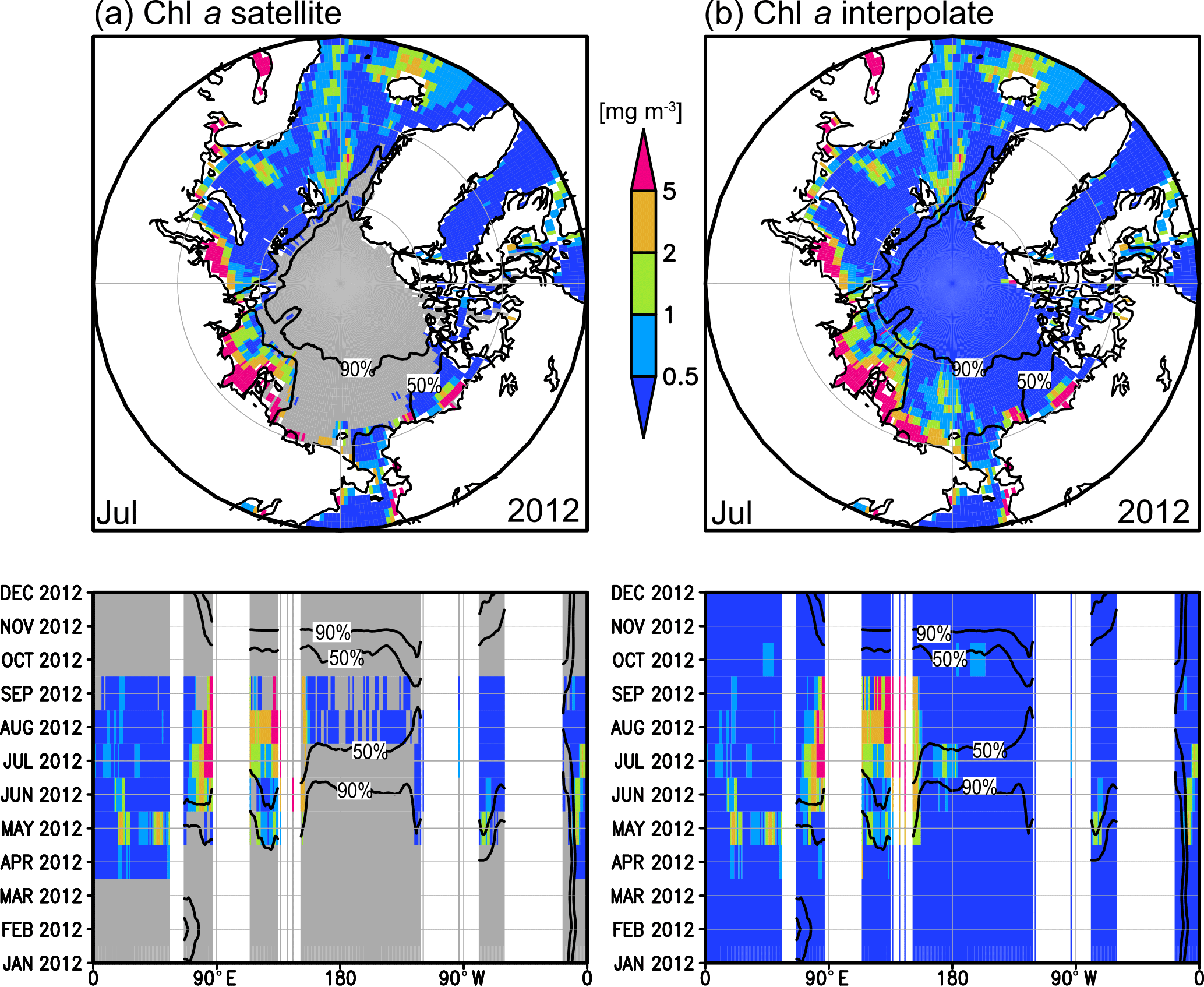
Figure 3 (a) Original and (b) interpolated Chl a (mg m⁻³) in July 2012 (upper panels), and along 75^∘ N in 2012 (lower panels). Black lines denote SIC of 50 and 90 %. Gray areas in (a) indicate missing Chl a data.

3.5 Calculation of air–sea CO₂ fluxes

We calculated monthly air–sea CO₂ flux (F) values from the pCO_2w values estimated in Sect. 3.4 by using the bulk formula:

$$\begin{array}{}\text{(2)}& F=kL(p{\mathrm{CO}}_{\mathrm{2}\mathrm{w}}-p{\mathrm{CO}}_{\mathrm{2}\mathrm{a}}),\end{array}$$

where k is the gas transfer velocity and L is the solubility of CO₂. The solubility of CO₂ (L) was calculated as a function of SST and SSS (Weiss, 1974). We converted the interpolated NOAA marine boundary layer xCO_2a data (Sect. 2.2) to pCO_2a by using monthly sea level pressure data and the water vapor saturation pressure calculated from monthly SST and SSS (Murray, 1967).

The gas transfer velocity k was calculated by using the formula of Sweeney et al. (2007):

$$\begin{array}{}\text{(3)}& k=\mathrm{0.19}(\mathit{\text{Sc}}/\mathrm{660}{)}^{-\mathrm{0.5}}\langle W_{\mathrm{NCEP}\mathrm{2}}^{\mathrm{2}}\rangle ,\end{array}$$

where Sc is the Schmidt number of CO₂ in seawater at a given SST, calculated according to Wanninkhof (1992, 2014), “〈〉” denotes the monthly mean, and $\langle W_{\mathrm{NCEP}\mathrm{2}}^{\mathrm{2}}\rangle$ is the monthly mean of the second moment of the NCEP2 6-hourly wind speed. The coefficient 0.19, which is the global average of $\mathrm{0.27}\langle W_{\mathrm{NCEP}\mathrm{1}}^{\mathrm{2}}\rangle /\langle W_{\mathrm{NCEP}\mathrm{2}}^{\mathrm{2}}\rangle$, is based on the one determined by Sweeney et al. (2007) but optimized for NCEP2 winds, following the same method as Schuster et al. (2013) and Wanninkhof et al. (2013).

The suppression of gas exchange by sea ice was accounted for by correcting the air–sea CO₂ fluxes using the parameterization presented by Loose et al. (2009); the flux is proportional to (1 − SIC)^0.4. Following Bates et al. (2006), in the regions with SIC > 99 %, we used SIC = 99 % to allow for non-negligible rates of air–sea CO₂ exchange through leads, fractures, and brine channels (Semiletov et al., 2004; Fransson et al., 2017). This parameterization reduces the flux in fully ice-covered waters (SIC > 99 %) by 84 %.

4 Uncertainty

4.1 Uncertainty in chlorophyll a concentration data

Figure 3 shows original and interpolated Chl a for the year 2012, as an example. Overall, the interpolated Chl a data seem to fit well with the original data. Most interpolated Chl a data have low concentrations because of high SIC and lack of sunlight. The average of the interpolated Chl a values is 0.1 mg m⁻³, and less than 5 % of the interpolated Chl a values are > 0.5 mg m⁻³ (cf. the average of the original Chl a values is 1.1 mg m⁻³, and 48 % of the original Chl a values are > 0.5 mg m⁻³). The previous studies to estimate pCO_2w in high latitudes assumed missing Chl a as constant values and ignored spatiotemporal variation in Chl a (Landschützer et al., 2013; Nakaoka et al., 2013). However, original Chl a values in the ice edge region are not small as captured by Perrette et al. (2011), and those in the northernmost grids in winter, north of which the original Chl a values are missing, are far south of the polar night region since they are missing not because of no sunlight but because of low angles of sunlight (Fig. 3a). Therefore, we believe interpolation is better than using low and constant values.

To validate our Chl a interpolation, we repeated the interpolation after randomly eliminating 10 % of the satellite Chl a values. We then used the eliminated original Chl a data as independent data for the validation. Note that this comparison was performed where there were the original Chl a data, i.e., the high Chl a region. The root mean square difference (RMSD) and correlation coefficient between the interpolated and the independent original Chl a data are 0.90 mg m⁻³ and 0.80, respectively. It means the interpolated Chl a, maybe not quantitatively, but qualitatively reproduced the original Chl a, and therefore is a meaningful parameter in the SOM process. Actually Chl a data improved the pCO_2w estimate, even though Chl a values in many grid cells were interpolated values (see Sect. 5.4).

Table 1 RMSD (mg m⁻³) and correlation (r) between Chl a values.

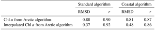
Figure 4 (a) Observed pCO_2w averaged over the whole analysis period (µatm). (b) Estimated pCO_2w averaged over the grid boxes in which observed pCO_2w values were available (µatm). (c) Bias (estimate–observation) and (d) RMSD between observed and estimated pCO_2w averaged over the whole analysis period (µatm).

Figure 5 (a) Monthly time series of observed pCO_2w averaged over the entire analysis area (black), and estimated pCO_2w averaged over the grid boxes in which observed pCO_2w values were available (green) (µatm). (b) Bias (estimate–observation; black) and RMSD (green) between observed and estimated pCO_2w averaged over the entire analysis area (µatm).

To evaluate our choice of Chl a algorithm (i.e., the Arctic algorithm of Cota et al., 2004), we compared its calculated Chl a values with those determined by using the standard algorithm of O'Reilly et al. (1998) and the coastal algorithm of Tassan (1994). RMSD and correlation coefficient (r) between the original (i.e., non-interpolated) Chl a values are about 0.8 mg m⁻³ and 0.9, respectively (Table 1). For all the Chl a values including the interpolated data, they are about 0.4 mg m⁻³ and 0.9. The lower RMSD in this case results from the fact that most of the interpolated Chl a values have low concentrations. This result means the Chl a from the different algorithms are, maybe not quantitatively, but qualitatively consistent with each other. Since not absolute Chl a values but relative values affect the pCO_2w estimates in the SOM technique, the large RMSD among the Chl a values does not result in significant difference of the pCO_2w estimates. Actually, the pCO_2w and CO₂ fluxes determined using Chl a from any of these algorithms as input to the SOM are consistent within their uncertainties (see Sect. 4.2 and 4.3 below). RMSDs between the observed and estimated pCO_2w are smallest in the pCO_2w estimate using Chl a from the Arctic algorithm, but the differences are quite small (< 1 %).

4.2 Uncertainty of pCO_2w mapping

Figure 4 compares observed and estimated pCO_2w (note that the spatial pattern visible in Fig. 4a and b includes differences generated by different seasonal coverage of data in the various regions). Both observed and estimated pCO_2w tend to be higher in the subpolar North Atlantic, the Laptev Sea, and the Canada Basin, and lower in the Greenland Sea and the Barents Sea. However, the east–west contrast in the Bering Sea and the contrast between the Canada Basin and the Chukchi Sea are weaker in our estimates than in the observations, and mean bias and RMSD are relatively large in those areas (Fig. 4c and d). The temporal changes in the observed and estimated pCO_2w are in phase (Fig. 5a), although the variability in the estimated values is somewhat suppressed compared to that of the observed data (note that the temporal change depicted in Fig. 5a also includes changes incurred by time variations in data coverage). The mean bias and RMSD fluctuate seasonally but are at a constant level over the years (Fig. 5b).

The correlation coefficient between estimated and observed pCO_2w is 0.82, and the RMSD is 30 µatm, which is 9 % of the average and 58 % of the standard deviation of the observed pCO_2w values. This is a performance level categorized as “good” by Maréchal (2004). The differences between the estimated and observed values stem not only from the estimation error but also from the error of the gridded observed data. The uncertainty of the pCO_2w measurements is 2–5 µatm (Bakker et al., 2014), the uncertainty of the pCO_2w values calculated from DIC and TA, whose uncertainties are within 4 and 6 µmol kg⁻¹, respectively (Olsen et al., 2016), can be up to 14 µatm (Lueker et al., 2000), and the sampling error of the gridded pCO_2w observation data was determined from the standard errors of monthly observed pCO_2w in the 1^∘ × 1^∘ grid cells to be 7 µatm (Yasunaka et al., 2016).

To validate our estimated pCO_2w values for periods and regions without any observed data, we repeated the mapping experiments after systematically excluding some of the observed pCO_2w data when labeling the neurons; four experiments were carried out, by excluding data (1) from 1997 to 2004, (2) from January to April, (3) from north of 80^∘ N, and (4) from the Laptev Sea (90–150^∘ E), where there are only a few pCO_2w observations. We compared the pCO_2w estimates obtained in each experiment with the excluded observations and found that the pCO_2w estimates reproduced the general features of the excluded data, both spatially and temporally (not shown here). They were also similar to the pCO_2w estimates obtained by using all observations, although the RMSDs between the estimates and the excluded observations are 54 µatm on average, which is 1.8 times the RMSDs of the estimates based on all observations. It means that our estimated pCO_2w values reproduce the general features both in space and time even when and where there are no observed data, although the uncertainty in pCO_2w might be as large as 54 µatm in regions and periods without data. We used this uncertainty for pCO_2w estimates made by using the pCO_2w values of a less similar neuron.

4.3 Uncertainty of CO₂ flux estimates

Signorini and McClain (2009) estimated the uncertainty of the CO₂ flux resulting from uncertainties in the gas exchange parameterization to be 36 % and the uncertainty resulting from uncertainties in the wind data to be 11 %. The uncertainty for SIC is 5 % (Cavalieri et al., 1984; Gloersen et al., 1993; Peng et al., 2013). The standard error of the sea ice effect on gas exchange was estimated to about 30 % by Loose et al. (2009). The uncertainty of pCO_2a is about 0.5 µatm (http://www.esrl.noaa.gov/gmd/ccgg/mbl/mbl.html), and that of pCO_2w was 30 µatm (Sect. 4.2); therefore, we estimated the uncertainty of ΔpCO₂ ($=p{\mathrm{CO}}_{\mathrm{2}\mathrm{w}}-p{\mathrm{CO}}_{\mathrm{2}\mathrm{a}}$) to be 34 % (average ΔpCO₂ in the analysis domain and period was −89 µatm). The overall uncertainty of the estimated CO₂ fluxes is thus 59 % ([0.36${}^{\mathrm{2}}+{\mathrm{0.11}}^{\mathrm{2}}+{\mathrm{0.05}}^{\mathrm{2}}+{\mathrm{0.3}}^{\mathrm{2}}+{\mathrm{0.34}}^{\mathrm{2}}{]}^{\mathrm{1}/\mathrm{2}})$ in sea-ice-covered regions and 51 % ([0.36${}^{\mathrm{2}}+{\mathrm{0.11}}^{\mathrm{2}}+{\mathrm{0.34}}^{\mathrm{2}}{]}^{\mathrm{1}/\mathrm{2}})$ in ice-free regions. For estimates using the pCO_2w values of a less similar neuron, whose uncertainty in pCO_2w is 54 µatm and the uncertainty of the ΔpCO₂ estimates can be as high as 61 %, the uncertainty is 78 % ([0.36${}^{\mathrm{2}}+{\mathrm{0.11}}^{\mathrm{2}}+{\mathrm{0.05}}^{\mathrm{2}}+{\mathrm{0.3}}^{\mathrm{2}}+{\mathrm{0.61}}^{\mathrm{2}}{]}^{\mathrm{1}/\mathrm{2}})$ in sea-ice-covered regions and 72 % ([0.36${}^{\mathrm{2}}+{\mathrm{0.11}}^{\mathrm{2}}+{\mathrm{0.61}}^{\mathrm{2}}{]}^{\mathrm{1}/\mathrm{2}})$ in ice-free regions. The average of the estimated CO₂ flux in the analysis domain and period is 4.8 $\mathrm{mmol}{\mathrm{m}}^{-\mathrm{2}}{\mathrm{d}}^{-\mathrm{1}}$; hence the uncertainty of the CO₂ flux estimate corresponds to 2.8 $\mathrm{mmol}{\mathrm{m}}^{-\mathrm{2}}{\mathrm{d}}^{-\mathrm{1}}$ in sea-ice-covered regions and 2.4 $\mathrm{mmol}{\mathrm{m}}^{-\mathrm{2}}{\mathrm{d}}^{-\mathrm{1}}$ in ice-free regions. For estimates using the pCO_2w values of a less similar neuron, the uncertainty corresponds to 3.7 $\mathrm{mmol}{\mathrm{m}}^{-\mathrm{2}}{\mathrm{d}}^{-\mathrm{1}}$ in the sea-ice-covered region and 3.5 $\mathrm{mmol}{\mathrm{m}}^{-\mathrm{2}}{\mathrm{d}}^{-\mathrm{1}}$ in ice-free regions.

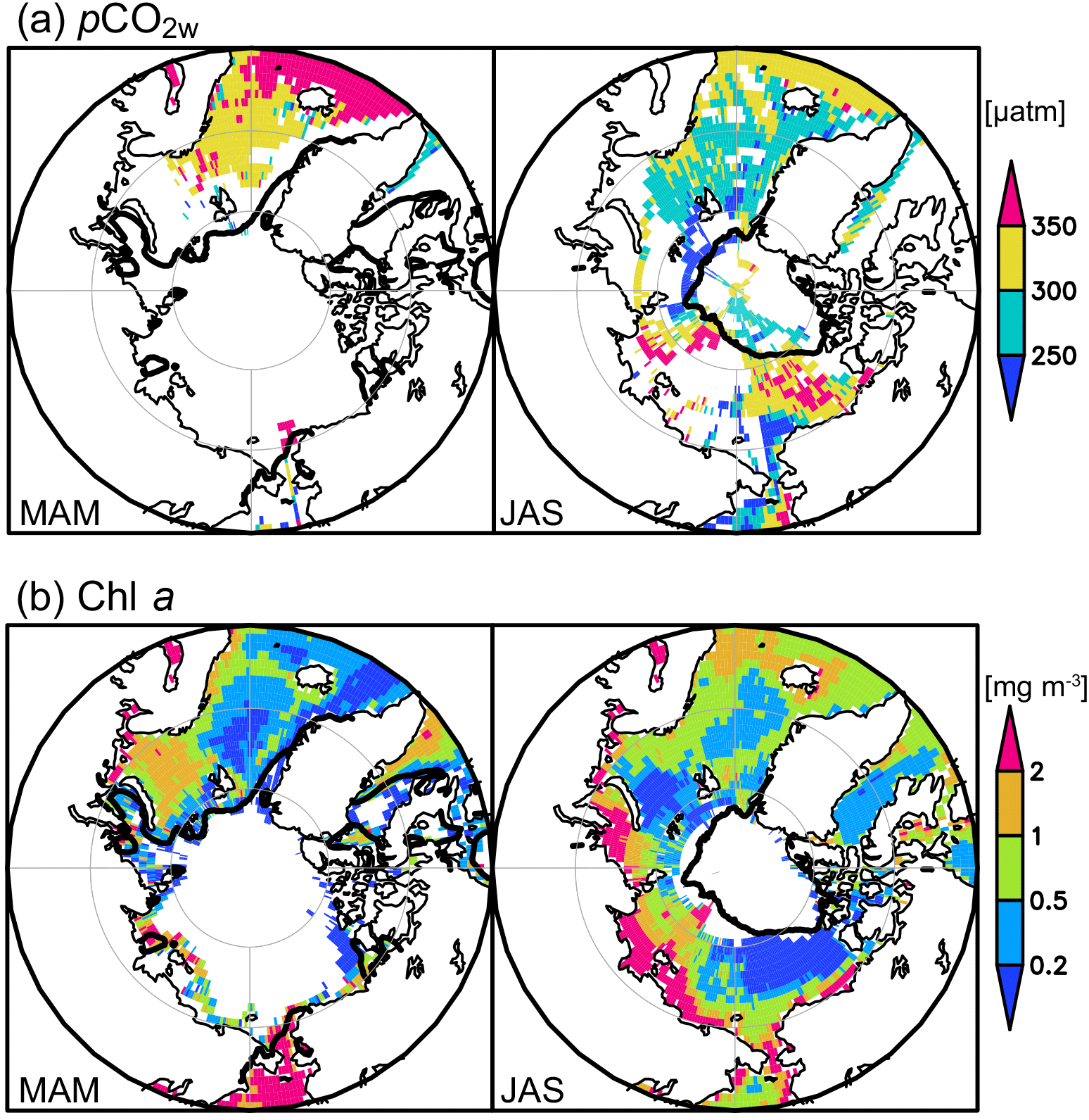
Figure 6 (a) Observed pCO_2w (µatm), and (b) non-interpolated Chl a (mg m⁻³) in March–May (left) and July–September (right) from 1997 to 2014.

5 Results and discussion

5.1 Relationship between pCO₂ and chlorophyll a

Figure 6 compares the observed pCO_2w and the original non-interpolated Chl a in spring (March–May) and summer (July–September). In spring, when much of the Arctic Ocean is ice covered, Chl a is high in the Barents Sea and the Bering Strait (> 1 mg m⁻³). In summer, when the ice cover is less extensive, Chl a is high in the Chukchi Sea, the Kara Sea, the Laptev Sea, and the East Siberian Sea (> 1 mg m⁻³) and especially high in the coastal regions of the two latter (> 2 mg m⁻³). pCO_2w is high in the Norwegian Sea in spring, and in the Kara Sea, the Laptev Sea, and the Canada Basin during summer (> 300 µatm). Conversely, it is lower in the Chukchi Sea, Bering Strait area, and the sea ice edge region of the Eurasian Basin in summer (< 300 µatm). The overall correlation between pCO_2w and Chl a is negative where Chl a ≤ 1 mg m⁻³ (70 % of all the data; correlation coefficient $r=-\mathrm{0.36}$, P < 0.01), but there is no significant relationship where Chl a > 1 mg m⁻³ (Fig. 7). A similar situation was identified in the subpolar North Atlantic by Olsen et al. (2008). It means that primary production generally draws down the pCO_2w, but high Chl a values are not necessarily associated with the low pCO_2w probably because high Chl a usually appears in the coastal regions (Fig. 6b; see below).

To determine the spatial variability in the relationship between pCO_2w and Chl a, we calculated the correlation coefficients between pCO_2w and Chl a in a window of ± 5^∘ of latitude and ± 30^∘ of longitude for each monthly 1^∘ × 1^∘ grid cell (Fig. 8a). The correlations between pCO_2w and Chl a are negative in the Greenland and Norwegian seas and over the Canada Basin. In the Greenland and Norwegian seas, the correlation between pCO_2w and Chl a is strongly negative ($r<-\mathrm{0.4}$) in spring and weakly negative (−0.4 < r < 0) in summer. Chl a there is higher in summer than in spring (Fig. 6b), whereas nutrient concentrations are high in spring and low in summer (Fig. 8b). Taken together, this suggests that primary production draws down the pCO_2w in spring, whereas in summer the primary production mostly depends on regenerated nutrients (Harrison and Cota, 1991) and the net CO₂ consumption is small, as also reported for the subpolar North Atlantic (Olsen et al., 2008). Therefore the correlation between pCO_2w and Chl a becomes less negative. In the eastern Barents Sea, the Kara Sea and the East Siberian Sea, and the Bering Strait, the correlations are positive because of water with high pCO_2w and Chl a in the coastal region subjected to river discharge (Murata, 2006; Semiletov et al., 2007; Anderson et al., 2009; Manizza et al., 2011). In the Chukchi Sea, the relationship is weak (−0.2 < r < 0.2), probably because the relationship is on smaller spatial and temporal scales than those represented by the window size used here, as shown by Mucci et al. (2010). The occurrence of calcifying plankton blooms in this region likely also weakens the correlation since the calcification increases pCO_2w (Shutler et al., 2013; Fransson et al., 2017).

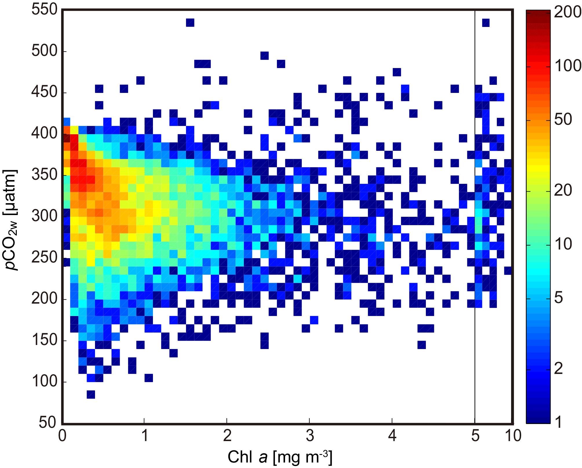
Figure 7 Observed pCO_2w (µatm) vs. satellite Chl a (mg m⁻³) in the Arctic Ocean and its adjacent seas (north of 60^∘ N) from 1997 to 2014. Colors indicate the number of data pairs in a 0.1 mg m⁻³ ×5 µatm bin when Chl a ≤ 5 mg m⁻³, or in a 1 mg m⁻³ × 5 µatm bin when Chl a > 5 mg m⁻³.

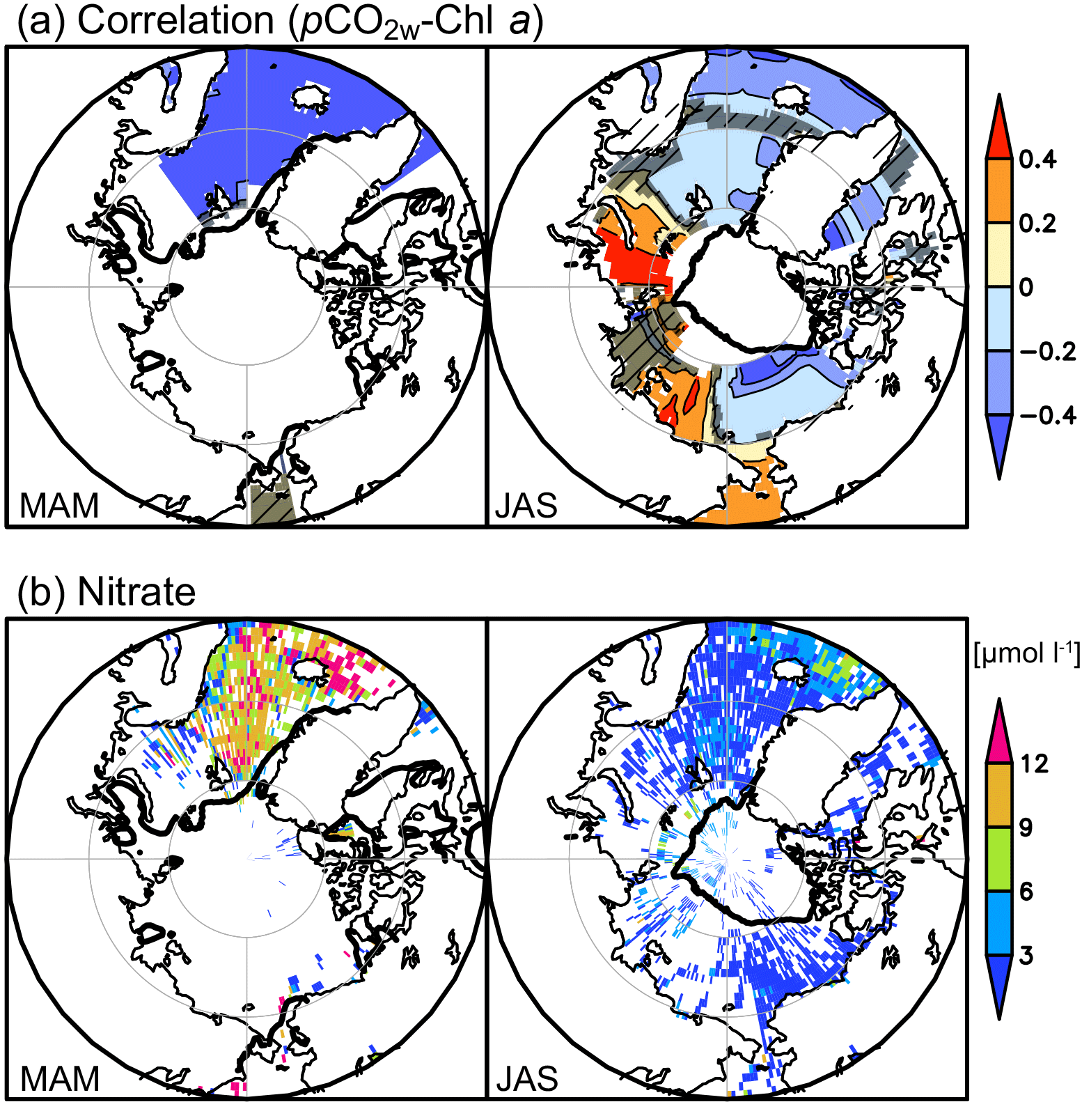
Figure 8 (a) Spatial correlation (correlation coefficient, r) between pCO_2w and Chl a in a window size of ± 1 month, ± 5^∘ latitude, and ± 30^∘ longitude in March–May (left) and July–September (right). Darker hatched areas represent values in grids where correlations are insignificant (P > 0.05). (b) Surface nitrate concentration (µmol L⁻¹) in March–May (left) and July–September (right) from 1997 to 2014.

These results show that pCO_2w relates to Chl a, but the relationships are different depending on the region and the season. It is difficult to represent such a complex relationship using simple equations (e.g., multiple regression methods) because it needs a priori assumptions of regression functions and of dividing the basin into subregions. But the SOM technique can empirically induce the relationships without any of the a priori assumptions and is therefore suitable to represent such a complex relationship.

5.2 Spatiotemporal CO₂ flux variability

The 18-year annual mean CO₂ flux distribution shows that all areas of the Arctic Ocean and its adjacent seas were net CO₂ sinks over the time period that we investigated (Fig. 9). The annual CO₂ influx to the ocean was strong in the Greenland and Norwegian seas (9 ± 3 $\mathrm{mmol}{\mathrm{m}}^{-\mathrm{2}}{\mathrm{d}}^{-\mathrm{1}}$; 18-year annual mean ± uncertainty averaged over the area shown in Fig. 1), the Barents Sea (10 ± 3 $\mathrm{mmol}{\mathrm{m}}^{-\mathrm{2}}{\mathrm{d}}^{-\mathrm{1}}$), and the Chukchi Sea (5 ± 3 $\mathrm{mmol}{\mathrm{m}}^{-\mathrm{2}}{\mathrm{d}}^{-\mathrm{1}}$). In contrast, influx was weak and not statistically significantly different from zero in the Eurasian Basin, the Canada Basin, the Laptev Sea, and the East Siberian Sea. Our annual CO₂ flux estimates are consistent with those reported by Yasunaka et al. (2016) and other previous studies (Bates and Mathis, 2009, and references therein).

The estimated 18-year average CO₂ influx to the Arctic Ocean was 5 ± 3 $\mathrm{mmol}{\mathrm{m}}^{-\mathrm{2}}{\mathrm{d}}^{-\mathrm{1}}$, equivalent to an uptake of 180 ± 130 Tg C yr⁻¹ for the ocean area north of 65^∘ N, excluding the Greenland and Norwegian seas and Baffin Bay (10.7 × 10⁶ km²; see Fig. 1). This accounts for 12 % of the net global CO₂ uptake by the ocean of 1.5 Pg C yr⁻¹ (Gruber et al., 2009; Wanninkhof et al., 2013; Landschützer et al., 2014). It is within the range of other estimates (81–199 Tg C yr⁻¹; Bates and Mathis, 2009), but close to the upper bound. That is partly because of the parameterization of the suppression effect by sea ice used in this study. Using another parameterization that represents the SIC effect linearly (Takahashi et al., 2009; Butterworth and Miller, 2016), CO₂ uptake of the Arctic Ocean was estimated to be 130 ± 110 Tg C yr⁻¹.

Figure 9 The 18-year annual means of CO₂ flux ($\mathrm{mmol}{\mathrm{m}}^{-\mathrm{2}}{\mathrm{day}}^{-\mathrm{1}}$) (negative values indicate flux into the ocean). Darker hatched areas represent values in grids where fluxes were smaller than the uncertainty, estimated as described in the text.

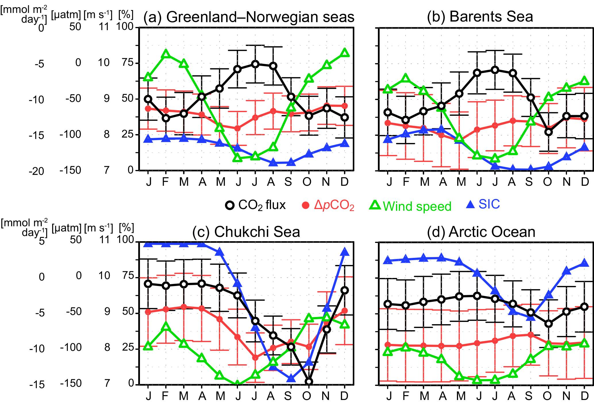
Figure 10 The 18-year monthly mean CO₂ flux ($\mathrm{mmol}{\mathrm{m}}^{-\mathrm{2}}{\mathrm{day}}^{-\mathrm{1}}$, black), ΔpCO₂ (µatm, red), wind speed (m s⁻¹, green), and SIC (%, blue), averaged over (a) the Greenland and Norwegian seas, (b) the Barents Sea, (c) the Chukchi Sea, and (d) the Arctic Ocean. Error bars indicate the uncertainty.

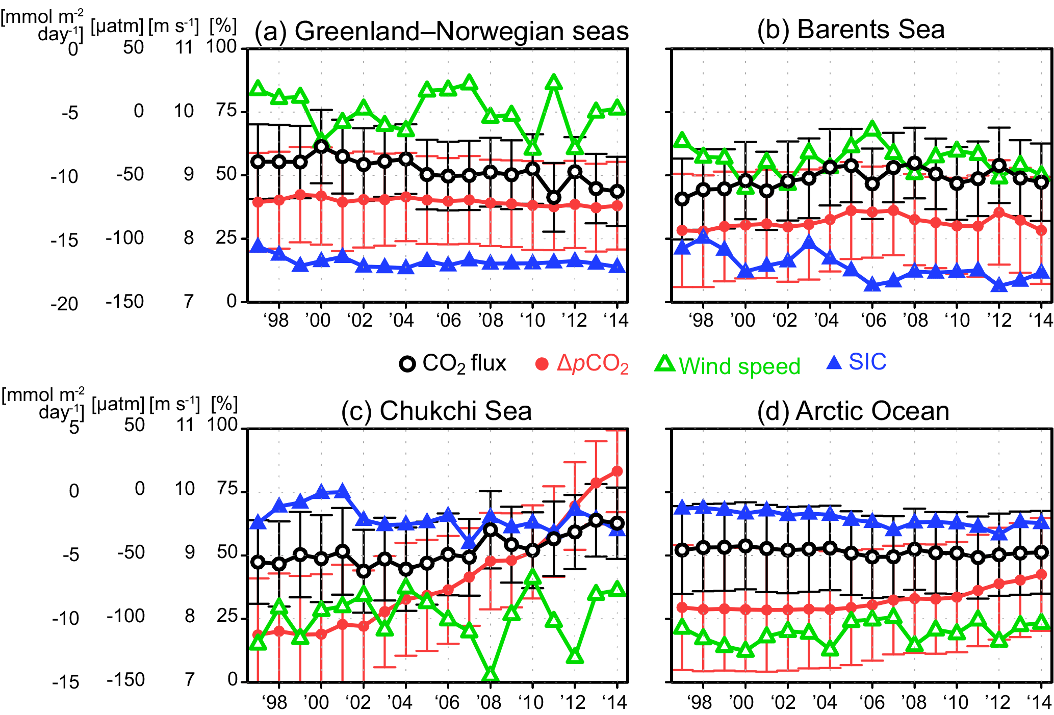
Figure 11 Area-mean interannual variations in CO₂ flux ($\mathrm{mmol}{\mathrm{m}}^{-\mathrm{2}}{\mathrm{day}}^{-\mathrm{1}}$, black), ΔpCO₂ (µatm, red), wind speed (m s⁻¹, green), and SIC (%, blue) in (a) the Greenland and Norwegian seas, (b) the Barents Sea, (c) the Chukchi Sea, and (d) the Arctic Ocean. Error bars indicate the uncertainty.

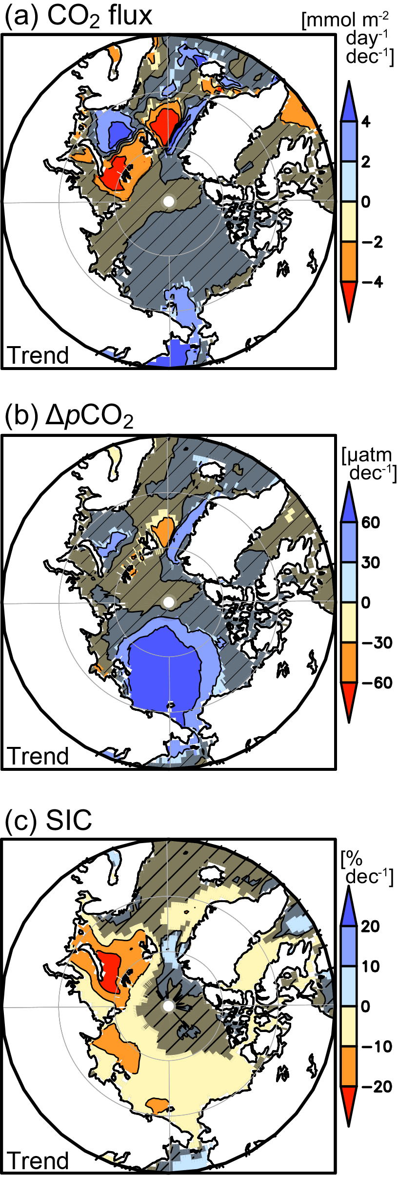
Figure 12 Trends in (a) CO₂ flux ($\mathrm{mmol}{\mathrm{m}}^{-\mathrm{2}}{\mathrm{day}}^{-\mathrm{1}}{\mathrm{decade}}^{-\mathrm{1}}$), (b) ΔpCO₂ (µatm decade⁻¹), and (c) SIC (% decade⁻¹). Darker hatched areas represent values in grids where trend values were less than the uncertainty, estimated as described in the text.

Figure 10 shows the seasonal variation in the air–sea CO₂ fluxes and its controlling factors (ΔpCO₂, wind speed and SIC; solubility is not shown as the impacts of its variations are relatively small in this context) in the Greenland and Norwegian seas, the Barents Sea, the Chukchi Sea, and the Arctic Ocean. In all of these regions the influxes are strongest in October, when the winds strengthen with the approach of winter and the pCO_2w and/or SIC are still as low as in the summer. In the Greenland and Norwegian seas and the Barents Sea the CO₂ influx shows a secondary maximum in February because the strongest winds occur in that month, while in the Chukchi Sea and Arctic Ocean, the winds are also strong but the flux is suppressed by the extensive sea ice cover. All of these regions are undersaturated with pCO_2w (i.e., negative ΔpCO₂) throughout all seasons. The undersaturation is strongest in the Arctic Ocean, as this has the most extensive sea ice cover limiting the fluxes from the atmosphere and the strongest stratification, limiting the mixing of CO₂ rich subsurface waters into the surface ocean. The undersaturation typically shows a maximum (i.e., ΔpCO₂ is minimum) in late spring to early summer (May–June) when the spring bloom occurs (Pabi et al., 2008), but not in the Arctic Ocean. Here the undersaturation reaches its minimum (ΔpCO₂ is the smallest) in late summer (August–September) at the time of minimum sea ice cover since the seasonal decrease in pCO₂ in summer is larger in the air than in the sea. Overall, in the Greenland and Norwegian seas and the Barents Sea the seasonal variations in the CO₂ flux are opposite to those expected from the seasonal ΔpCO₂ variations because it is the wind speed that governs most of the seasonal flux variations. In the Chukchi Sea, however, the CO₂ influx is strongest in summer, a consequence of the minimum sea ice cover and strongest pCO₂ undersaturation. In the Arctic Ocean it is the SIC and wind speed that drive the seasonal flux variations. Seasonal variations in CO₂ flux are consistent with those of the previous studies (Yasunaka et al., 2016, and references therein), whereas seasonal variations in pCO_2w become realistic (see Sect. 5.3 below).

Figure 11 shows interannual variation in CO₂ flux and its driving factors in these four regions. The interannual variations in CO₂ flux and ΔpCO₂ are generally smaller than the seasonal variations and are often smaller than their respective uncertainty. In the Greenland and Norwegian seas, interannual variation in the CO₂ flux negatively correlates with the wind speed (CO₂ influx to the ocean is large when the wind is strong; $r=-\mathrm{0.41}$), while interannual variation in ΔpCO₂ and sea ice change is small. In the Barents Sea, the interannual variation in CO₂ flux positively correlates with ΔpCO₂ (r=0.71) and negatively correlates with SIC ($r=-\mathrm{0.50}$), while the correlation with wind speed is not significant. Although low SIC enhances the air–sea CO₂ exchange due to increase in the area of open water, it also associates with high SST and therefore high pCO_2w. In the Chukchi Sea, CO₂ influx to ocean is decreasing with increasing ΔpCO₂ (r=0.87). High pCO_2w (> 500 µatm) via storm-induced deep mixing events has been sometimes observed in the Chukchi Sea after 2010 (Hauri et al., 2013; Taro Takahashi, personal communication, 2017). Interannual variability in the CO₂ flux averaged over the Arctic Ocean is small because the increasing ΔpCO₂ is compensated for by the effect of sea ice retreat ($r=-\mathrm{0.70}$). Thus, the combined effect of sea ice retreat and pCO_2w increase on CO₂ flux varied among regions.

The CO₂ influx has been increasing in the Greenland Sea and northern Barents Sea and decreasing in the Chukchi Sea and southern Barents Sea (Fig. 12). The CO₂ flux trend corresponds well with the ΔpCO₂ trend, which in turn corresponds well with the SST trend. The increasing CO₂ influx in the northern Barents Sea also corresponds with the sea ice retreat. These results are similar to those for the previous estimates without using Chl a (see Fig. 10 in Yasunaka et al., 2016). It shows again that the combined effect of sea ice retreat and pCO_2w increase on the CO₂ flux is regionally different. In the SOM process, the pCO_2w values observed in the latter period might be used for the pCO_2w estimate in the former period when the pCO_2w measurements have not been made, and therefore the trend in CO₂ influx might be affected by the spatiotemporal distribution of the measurements. To confirm this is not the case, we checked that the spatial distribution of the pCO_2w trend did not correspond to the year when the first observation was conducted (see Supplement).

Figure 13 The 18-year averaged pCO_2w seasonal variations (µatm) in (a) the Greenland and Norwegian seas, (b) the Barents Sea, and (c) the Chukchi Sea. Black lines with triangles show estimates without Chl a; magenta lines with open circles show estimates with Chl a; green lines with closed circles show observed values. The upper panels show pCO_2w averaged for all grid cells within each region, and the lower panels show pCO_2w averaged over the grid boxes in which observed pCO_2w values were available. Error bars show the uncertainty, estimated as described in the text.

5.3 Impact of incorporating chlorophyll a data in the SOM

To determine the impact of including Chl a data in the SOM process, the analyses were repeated without Chl a data. The RMSD of the resulting estimated pCO_2w values is 33 µatm, which is 3 µatm larger than the uncertainty of the estimates generated by including Chl a in the SOM. Chl a data thus improved the pCO_2w estimate (namely, a 10 % reduction of RMSD), even though 40 % of the Chl a data labeled with pCO_2w observations were interpolated Chl a values.

Figures S1 and S2 in the Supplement present the difference in bias and RMSD for pCO_2w estimated with and without Chl a; Fig. S1 shows the time evolution and Fig. S2 shows the spatial distribution. Both approaches typically underestimate pCO_2w in winter and overestimate the summertime values, but these systematic biases are reduced when Chl a values are included in the SOM (Fig. S1). Biases and RMSDs are reduced in the Canada Basin, the western Bering Sea, and the boundary region between the Norwegian Sea and the subpolar North Atlantic (Fig. S2). As a result, the strong east–west contrast in the Bering Sea and the contrast between the Canada Basin and the Chukchi Sea (see Fig. 4) are better represented when Chl a is included. Taken together, inclusion of Chl a when estimating pCO_2w yields not only better representation of the pCO_2w decline in spring and summer but also improves the representation of the spatiotemporal pCO_2w distribution. Technically, these improvements come from the fact that Chl a as a training parameter can separate high Chl a region–time and low Chl a region–time into different neurons, which were combined into the same neurons trained without Chl a. For example, since Chl a is high in spring but SST and SIC are still at similar levels as winter, the grid cells in spring and winter would be classified into separate neurons when Chl a is included as a training parameter but in the same neuron when Chl a is not included. As a result, without Chl a, the estimated pCO_2w in spring tends to be similar to the pCO_2w in winter, and the pCO_2w in winter tends to be similar to that in spring. And therefore the contrast between winter and spring is weakened without Chl a.

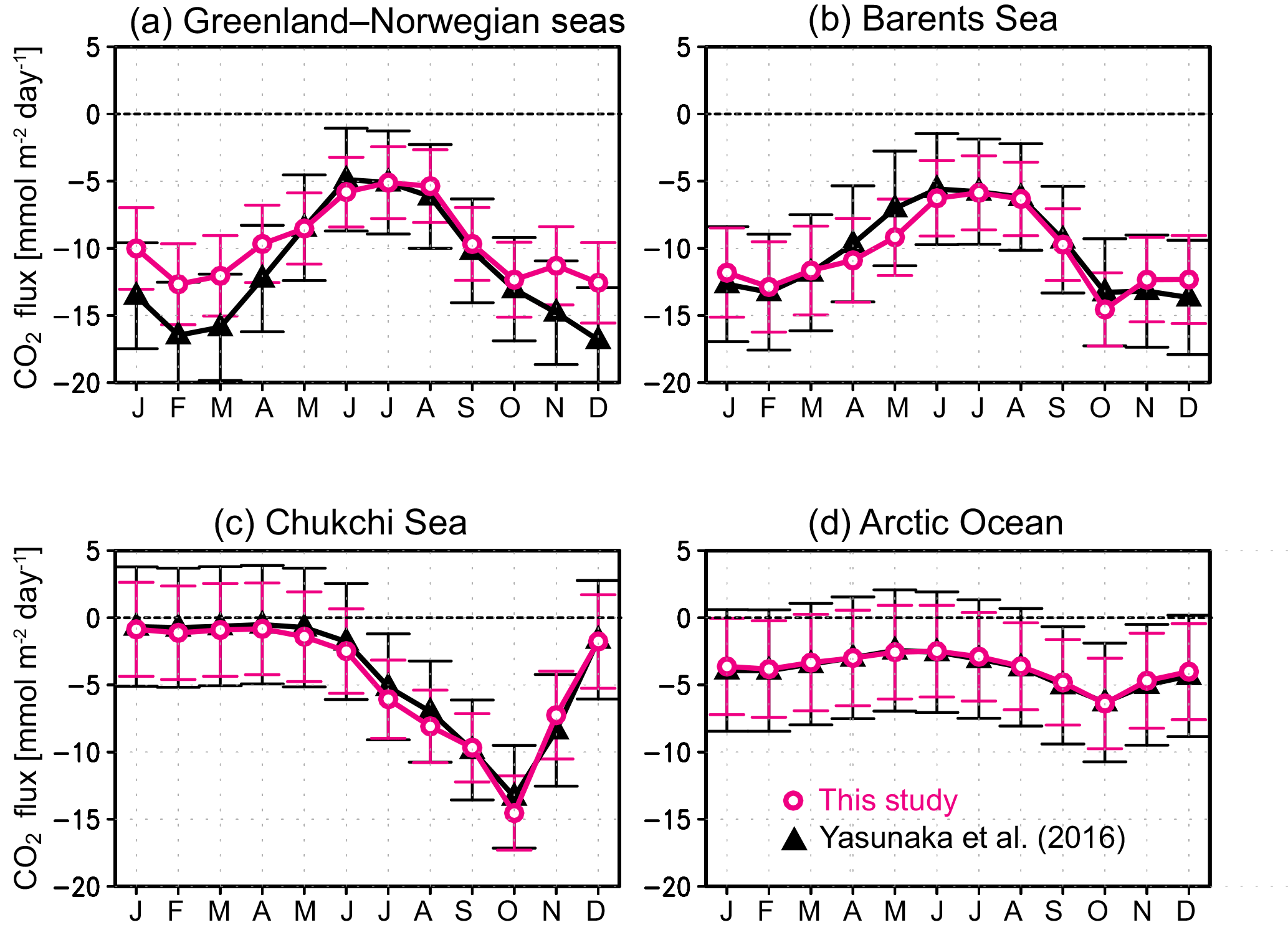
Figure 14 The 18-year monthly mean CO₂ flux ($\mathrm{mmol}{\mathrm{m}}^{-\mathrm{2}}{\mathrm{day}}^{-\mathrm{1}}$) averaged over (a) the Greenland and Norwegian seas, (b) the Barents Sea, (c) the Chukchi Sea, and (d) the Arctic Ocean. Black lines with triangles show estimates without Chl a by Yasunaka et al. (2016); magenta lines with open circles show estimates with Chl a. Error bars show the uncertainty, estimated as described in the text.

The seasonal cycles of pCO_2w estimates derived with the inclusion of Chl a have a larger amplitude than the uncertainties, whereas the uncertainties are larger than the seasonal amplitude when pCO_2w is derived without Chl a (upper panels of Fig. 13). The difference is caused by the fact that the seasonal cycle of pCO_2w in each region reproduces the observed cycle better when Chl a was included (lower panels of Fig. 13). Note that the much larger seasonal amplitude in the lower panels is an artefact generated by the seasonal bias in sampling locations; in winter most measurements are obtained at low latitudes where pCO_2w is typically higher than at high latitudes.

Compared to the CO₂ influx estimates by Yasunaka et al. (2016), the winter CO₂ influx in the Greenland and Norwegian seas estimated including Chl a is about 3 $\mathrm{mmol}{\mathrm{m}}^{-\mathrm{2}}{\mathrm{d}}^{-\mathrm{1}}$ less than that calculated without using Chl a (Fig. 14), but this difference is smaller than the uncertainties. The CO₂ fluxes in the other areas are quite similar for the two estimates, while their uncertainties are smaller in the present estimates.

The inclusion of Chl a data also reduced the uncertainty of the estimated annual air–sea CO₂ flux integrated over the entire Arctic Ocean. Compared to the flux estimate determined by Yasunaka et al. (2016) of 180 ± 210 Tg C yr⁻¹, the CO₂ uptake in the Arctic Ocean estimated here is significant within its uncertainty (180 ± 130 Tg C y⁻¹). This improvement is the result of (1) the inclusion of Chl a data in the SOM process (which reduced the uncertainty by 23 %); (2) the separate uncertainty estimates for ice-free and ice-covered regions (8 %); and (3) the addition of new observational pCO_2w data (7 %). Reducing the uncertainty of this quantification is a key contribution to the larger work of constraining the global carbon budget (e.g., Le Quéré et al., 2016). Because the Arctic is an important CO₂ sink, quantifying its fluxes and minimizing the uncertainty is of great scientific value.

5.4 Toward further reduction of the uncertainty

The addition of new observational data from SOCATv4 and GLODAPv2 reduced the overall uncertainty in the mapped pCO_2w: a 33 % increase in the number of observations induced a 7 % reduction in the uncertainty. However, there are still few observations in the Kara Sea, the Laptev Sea, the East Siberian Sea, and the Eurasian Basin (Fig. 2). To improve our understanding of the variability in air–sea CO₂ fluxes in the Arctic, it is of critical importance to obtain additional ocean CO₂ measurements to fill these data gaps and that these measurements are made publically available. Data synthesis activities like SOCAT must be encouraged.

In the present study, we discussed the combined effect of sea ice retreat and pCO_2w change on the air–sea CO₂ flux. There are other factors that will induce change of CO₂ flux. For example, warmer temperature will lead to an increasing buffering capacity while lower salinity will have the opposite effect and cause a decrease in buffering capacity. In our current study, we used climatological-mean salinity for the pCO_2w estimate because of lack of reliable year-to-year salinity data. That might be one of the improvements for a future study.

6 Conclusions

By applying an SOM technique with the inclusion of Chl a data to estimate pCO_2w, we produced monthly maps of air–sea CO₂ fluxes from 1997 to 2014 for the Arctic Ocean and its adjacent seas north of 60^∘ N. Negative correlation between pCO_2w and Chl a meant that Chl a is a valuable parameter to represent primary production. Since the relationship varied among seasons and regions, the SOM technique is better suited for the mapping than a multiple linear regression approach. Adding Chl a to the SOM process improved representation of the seasonal cycle of pCO_2w and therefore reduced the uncertainty of the CO₂ flux estimates.

In the Greenland and Norwegian seas and the Barents Sea the CO₂ influx was large in autumn and winter because of the strong wind. In the Chukchi Sea, however, the CO₂ influx was strong in summer and autumn, as a consequence of the low SIC and strong pCO_2w undersaturation. Although interannual variation in the CO₂ influx was smaller than the seasonal variation, the CO₂ influx has been increasing in the Greenland Sea and northern Barents Sea and decreasing in the Chukchi Sea and southern Barents Sea.

A major goal of the carbon-cycle research community in recent years has been to reduce the uncertainty in estimates of carbon reservoirs and fluxes. Our results contribute to this in that CO₂ uptake in the Arctic Ocean is demonstrated with high significance. The resulting estimate of the annual Arctic Ocean CO₂ uptake of 180 Tg C yr⁻¹ is significant with an uncertainty of ± 130 Tg C yr⁻¹. This is a substantial improvement over earlier estimates and is due mainly to the incorporation of Chl a data.

Assessment of the numerical models using our estimate of Arctic carbon uptake is also an interesting topic since numerical models are poorly validated in the Arctic due to the limited observations of biogeochemistry (Popova et al., 2012). However, such experiments need thorough insight into the numerical models, which is beyond the scope of this study. We hope to perform such comparisons in future studies.