the Creative Commons Attribution 4.0 License.
the Creative Commons Attribution 4.0 License.
 | 17 Oct 2019
N2O changes from the Last Glacial Maximum to the preindustrial – Part 1: Quantitative reconstruction of terrestrial and marine emissions using N2O stable isotopes in ice cores
Hubertus Fischer
Jochen Schmitt
Michael Bock
Barbara Seth
Fortunat Joos
Renato Spahni
Sebastian Lienert
Gianna Battaglia
Benjamin D. Stocker
Adrian Schilt
Edward J. Brook
Using high-precision and centennial-resolution ice core information on atmospheric nitrous oxide concentrations and its stable nitrogen and oxygen isotopic composition, we quantitatively reconstruct changes in the terrestrial and marine N2O emissions over the last 21 000 years. Our reconstruction indicates that N2O emissions from land and ocean increased over the deglaciation largely in parallel by 1.7±0.3 and 0.7±0.3 TgN yr−1, respectively, relative to the Last Glacial Maximum level. However, during the abrupt Northern Hemisphere warmings at the onset of the Bølling–Allerød warming and the end of the Younger Dryas, terrestrial emissions respond more rapidly to the northward shift in the Intertropical Convergence Zone connected to the resumption of the Atlantic Meridional Overturning Circulation. About 90 % of these large step increases were realized within 2 centuries at maximum. In contrast, marine emissions start to slowly increase already many centuries before the rapid warmings, possibly connected to a re-equilibration of subsurface oxygen in response to previous changes. Marine emissions decreased, concomitantly with changes in atmospheric CO2 and δ13C(CO2), at the onset of the termination and remained minimal during the early phase of Heinrich Stadial 1. During the early Holocene a slow decline in marine N2O emission of 0.4 TgN yr−1 is reconstructed, which suggests an improvement of subsurface water ventilation in line with slowly increasing Atlantic overturning circulation. In the second half of the Holocene total emissions remain on a relatively constant level, but with significant millennial variability. The latter is still difficult to attribute to marine or terrestrial sources. Our N2O emission records provide important quantitative benchmarks for ocean and terrestrial nitrogen cycle models to study the influence of climate on nitrogen turnover on timescales from several decades to glacial–interglacial changes.
- Article
(8052 KB) - Full-text XML
- Companion paper
- BibTeX
- EndNote


Nitrous oxide (N2O) is an important greenhouse gas that contributes to ongoing and past global warming (Stocker et al., 2013; Schilt et al., 2010b) and is involved in the destruction of stratospheric ozone (Myhre et al., 2013). Its past atmospheric variations are recorded in polar ice cores, although some sections of some records can be affected by in situ formation of N2O. N2O is produced through nitrification and denitrification on land and in the ocean, but nitrification appears to be the dominant pathway in marine environments (Battaglia and Joos, 2018b). Total natural net N2O sources are estimated to amount to 10.5±1 TgN yr−1, where about 60 % are estimated to be of terrestrial origin (Battaglia and Joos, 2018b), very similar to IPCC AR5 terrestrial emission estimates of 6.6 (3.3 to 9.0) TgN yr−1. Atmospheric N2O is photochemically destroyed in the stratosphere (Ciais et al., 2013) with an estimated preindustrial lifetime of 123 years (Prather et al., 2015).
Reconstructions of past variations in terrestrial and marine N2O emissions from ice core data (Schilt et al., 2014) provide information on the response of the global coupled carbon–nitrogen cycle to past climate variations. Atmospheric N2O increased from 270 ppb (MacFarling Meure et al., 2006) to around 330 ppb (https://www.esrl.noaa.gov/gmd/, last access: 11 October 2019) over the industrial period due to human activities such as fertilizer applications (Bouwman et al., 2013; Ciais et al., 2013). Atmospheric N2O varied between natural upper and lower bounds of around 300 and 180 ppb, respectively, over glacial–interglacial cycles (Sowers et al., 2003; Spahni et al., 2005; Schilt et al., 2010a). Moreover, atmospheric N2O concentrations showed a clear positive imprint of rapid climate warmings in the North Atlantic region that occurred during the last ice age (so called Dansgaard Oeschger (DO) events) and during the last glacial–interglacial transition (the Bølling–Allerød (BA) warming and the rapid warming at the end of the Younger Dryas (YD) into the Preboreal (PB)). These rapid warming events have been shown to be associated with a resumption of the Atlantic Meridional Overturning Circulation (AMOC) (Henry et al., 2016; Pedro et al., 2018; McManus et al., 2004) and a connected northward shift of the Intertropical Convergence Zone (ITCZ) leading to significant changes in monsoon precipitation (Wang et al., 2008). Available N2O data over the Holocene also show significant albeit smaller longer-term N2O variability. Until recently it had not been possible to attribute the observed concentration changes to terrestrial or marine sources, and ecosystem and physical processes leading to changes in N2O production remained not well understood.
Using the different nitrogen isotopic signature of terrestrial and marine N2O sources, high-resolution data on the isotopic composition of N2O from Greenland and Antarctic ice cores allow us to reconstruct past variations in terrestrial and marine N2O emissions and, thus, on C–N coupling on timescales from several decades to many centuries. A recent ice core study on the stable isotope composition of N2O over the time interval from 16 000 to 10 000 years before present (ka BP, where present is defined as 1950) demonstrated the power of such an isotopic approach (Schilt et al., 2014). The isotopic data showed that both land and marine sources increased during the interval from 16 to 10 ka BP and showed a clear imprint of AMOC variations and related climate changes on the terrestrial and marine carbon and nitrogen cycles (Schilt et al., 2014). Here we attempt a more detailed look at the temporal evolution and phasing of marine and terrestrial N2O emissions over this time interval. No previous study was able yet to reconstruct the complete temporal evolution in terrestrial versus marine emissions of N2O since the Last Glacial Maximum (LGM; 21 ka BP, including the onset of the termination and the early deglacial “Mystery Interval”) and to reconstruct the more subtle changes in the course of the Holocene.
Accordingly, the aim of this study is to improve our understanding of the changes in the main N2O sources over these time intervals. In this study we reconstruct the emissions of N2O from land and from the ocean over the entire glacial termination and the Holocene, using new ice core N2O isotope data. We contrast these emission changes to the accompanying changes in climate parameters and ocean circulation as archived in ice cores and marine sediments. In the accompanying paper (Joos et al., 2019a) these new emission records of the past 21 kyr are used to explore and test alternative mechanisms of the functioning of the C–N cycle on land and to quantify the leading environmental parameters controlling land-based N2O emissions over this time interval, while the response of the marine nitrogen cycle to rapid changes in AMOC has been recently studied by several coupled biogeochemistry ocean models (Schmittner and Galbraith, 2008; Joos et al., 2019b; Goldstein et al., 2003).
2.1 Composite records of N2O, δ15N(N2O) and δ18O(N2O) from bipolar ice cores
2.1.1 New N2O concentration and dual isotope measurements
A total of 202 ice core samples were analyzed at the University of Bern for N2O and its nitrogen and oxygen isotopic composition and compiled with previously published N2O isotope data measured at Oregon State University over the time interval 16 to 10 ka BP (Schilt et al., 2014). We measured 103 samples on ice from the North Greenland Ice Core Project (NGRIP), 42 from the European Project for Ice Coring in Antarctica (EPICA) Dronning Maud Land core (EDML), and 57 from the Antarctic Talos Dome Ice Core (TALDICE). A subset of 13 samples of these 202 samples are considered to be affected by in situ production of N2O (7 for NGRIP, 5 for EDML, and 1 for TALDICE) and were excluded from our data set (see details on outlier detection below).
The new data cover the period from about 27 to 0.3 ka BP and allow us to reconstruct for the first time the N2O isotopic composition for the LGM, the early deglacial period, and the entire Holocene (last 11 kyr). Two independent analytical systems were used at the University of Bern for both δ15N(N2O) and δ18O(N2O) as described in detail previously (Bock et al., 2014; Schmitt et al., 2014). δ15N(N2O) data are given with respect to atmospheric N2, δ18O(N2O) data are reported with respect to VSMOW (Vienna Standard Mean Ocean Water), both in the commonly used delta notation. Our reference is a recent air sample, NAT332, measured at Utrecht University (Sapart et al., 2011) and cross-referenced to Air Controlé, an in-house standard in Bern (Schmitt et al., 2014). Finally, all new Bern data presented here are shifted by small, constant offsets (−0.80 ‰ for δ15N(N2O) and +0.36 ‰ for δ18O(N2O)) to account for laboratory differences among results measured at the University of Bern and at Oregon State University as described previously (Schilt et al., 2014).
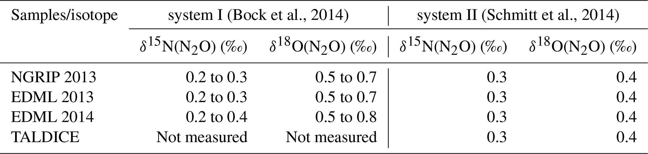
The analytical precision for the two systems used at the University of Bern and for different sample batches is given in Table 1. Error bars of all isotopic data in this publication represent one standard deviation (±1σ) of ice sample replicates or are based on the reproducibility of air reference measurements used to calibrate ice samples. Measurement precisions of individual samples for N2O, δ15N(N2O) and δ18O(N2O) are always better than ±5 ppb, ±0.4 ‰ and ±0.8 ‰, respectively (Table 1).
Table 1Measurement precision (±1 standard deviation) of N2O isotope ice core data measured at the University of Bern in this study.
2.1.2 The composite ice core records – data and age scale
Using measurements performed on various Greenland and Antarctic ice cores, composite records for N2O concentration and dual isotope signatures were derived over the last up to 28 kyr (Fig. 1). To this end our new N2O concentration data were combined with published N2O concentration data from NorthGRIP (Schilt et al., 2010b) after exclusion of data points likely affected by in situ N2O formation (see below), EPICA Dome C (EDC) (Flückiger et al., 2002; Spahni et al., 2005), and Taylor Glacier ice (Schilt et al., 2014). The EDC data included are for ages younger than 14.5 ka BP and the published Taylor Glacier data (Schilt et al., 2014) cover the period from 15.9 to 9.9 ka BP. We do not include published N2O concentration data from previous Talos Dome measurements (Schilt et al., 2010b) in the composite due to unresolved analytical offsets between these published and our new N2O concentration data. The new N2O dual isotope data are combined with published N2O dual isotope data from Taylor Glacier (Schilt et al., 2014) measured at Oregon State University covering the period 15.9 to 9.9 ka BP; the analytical procedures at Oregon and Bern are tightly cross-calibrated (Schilt et al., 2014; Schmitt et al., 2014).

Figure 1Compilation of new and published N2O records over the last 28 kyr including identified artifacts due to in situ production of N2O. (a) N2O concentration from this study and published records (Sowers et al., 2003; Bernard et al., 2006; Flückiger et al., 2002; MacFarling Meure et al., 2006; Park et al., 2012; Schilt et al., 2010b; Schmitt et al., 2014) (b) δ15N(N2O) and (c) δ18O(N2O) from this study and published records (Sowers et al., 2003; Bernard et al., 2006; Park et al., 2012; Schmitt et al., 2014; Schilt et al., 2014). The solid lines in (a)–(c) represent Monte Carlo average smoothing splines with a cutoff period of 2000 years prior to 16 ka BP and 700 years afterwards. The grey shaded envelopes (±2σ) represent the Monte Carlo based uncertainties of the splines. Samples identified to be subject to in situ formation are indicated by red circles; extreme values outside the plotting range are indicated by arrows and provided in small orange boxes.
In order to compare N2O data from different ice records, they must be put on a common age scale. We start from the existing AICC2012 age scale (Veres et al., 2013) and compare the concentrations of the fast-varying and globally well-mixed greenhouse gas methane (CH4) between ice cores (Fig. 2). In the process of establishing the AICC2012 age scale, Greenland and Antarctic ice cores were synchronized by aligning rapid climate changes in Greenland δ18O with rapid CH4 variations in Antarctic ice cores (Veres et al., 2013). Unfortunately, due to the ice age–gas age difference between Greenland δ18O and CH4 records, this leaves some uncertainty when comparing Greenland and Antarctic gas records. Accordingly, new high-resolution CH4 data reveal that AICC2012 gas ages are offset by several hundred years at the start of the BA and before and after the YD (Fig. 2). This is also true for other time periods during the last glacial period (Baumgartner et al., 2014), where rapid CH4 increases occurred. To correct for this age offset, we match mid points of fast CH4 variations (BA and YD) seen in all our ice cores to the fast climatic changes indicated by δ18O at NGRIP on the absolutely counted GICC05 age scale (Rasmussen et al., 2006). This assumes that the CH4 response is synchronous with rapid climate changes within a few decades, as previously shown for the NGRIP ice core (Baumgartner et al., 2014).
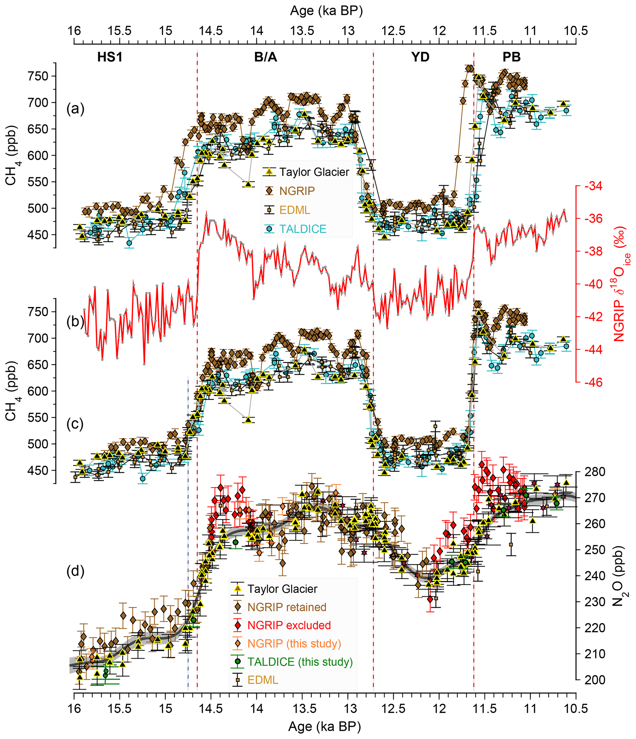
Figure 2Methane synchronization of ice core records. (a) Existing methane (CH4) concentration records for NGRIP and EDML (Baumgartner et al., 2012), and TALDICE (Schilt et al., 2010b) shown on the original AICC2012 gas age scale. The fast climate variations indicated by the NGRIP δ18Oice record (b) (Rasmussen et al., 2006) were used as tie points for CH4 changes in the NGRIP and TALDICE ice cores (mid points of the CH4 changes indicated by vertical dashed red lines). The onset of the CH4 increase at the end of HS1 is indicated by the blue vertical dashed line (see text). A similar approach had been taken by Schilt et al. (2010b) by synchronizing the fast changes in the Taylor Glacier CH4 data with the corresponding changes in the WAIS Divide deep ice core CH4 data on an updated version of the WDC06A-7 timescale. The synchronized CH4 records (c) are then used to create a common gas age scale for N2O data on the GICC05 age scale (d) (Rasmussen et al., 2006).
A well-known problem with N2O data is that they can be subject to in situ N2O formation for some ice core sections. In situ production leads to elevated N2O concentrations and abnormal isotopic signatures compared to other, coeval, ice core records. For Greenland ice, in situ artifacts typically occur as erratic N2O outliers during the glacial, especially when the ice chemistry changes during major climatic transitions (see Fig. 1; measurements with identified in situ production are marked by red circles). For several Antarctic ice cores (Schilt et al., 2010b; Flückiger et al., 2004, 1999), the dust-rich LGM sections are almost entirely affected by in situ production (see EDC and EDML records in Fig. 1). Due to their lower impurity content, the TALDICE ice core as well as the outcropping ice from Taylor Glacier (Schilt et al., 2014) appear to be an exception and potential artifacts have been found only in very few instances (Schilt et al., 2010b).
The most straightforward criterion to identify samples affected by in situ production targets anomalies in the N2O concentration. The assumption is that N2O cannot be consumed or lost in the ice, but only produced. An outlier detection method was used for the highest-resolution N2O record available to date (both in sample frequency and in terms of the width of the bubble enclosure characteristics) from the Greenland NGRIP ice core (Schilt et al., 2013) covering the time interval from 110 to 10 ka BP. Individual samples in this record were removed if they exceeded a threshold of 8 ppb above a spline approximation through all samples (Flückiger et al., 2004). This outlier algorithm is not well suited for detecting in situ formation in times when N2O concentrations increase strongly due to rapid emission increases. Thus, the outlier detection may fail during the onset and end of DO events. In fact, as illustrated in Fig. 2, the published NGRIP N2O record appears to be systematically higher than its Antarctic counterparts from the Talos Dome ice core and from Taylor Glacier after the onset of the BA and after the end of the YD, although the long atmospheric lifetime of N2O requires an interhemispheric gradient below the range of the measurement uncertainty. The higher NGRIP concentrations in these intervals can also not be attributed to narrower bubble enclosure characteristics and thus better resolution of the record compared to the Antarctic data, as the concurrent increase in atmospheric CH4 concentrations is comparably rapid in the NGRIP and Taylor Glacier data (Fig. 2). Accordingly, we cannot exclude an in situ contribution to the rapid N2O increases in the NGRIP ice core and excluded the respective samples (red symbols in Fig. 2) from our data set.
To obtain a final data set compiled from all cores after the pre-screening described above and to rigorously remove samples that may still be affected by in situ processes, individual samples were finally excluded in our study from the data set compiled from all ice cores if they were at least 20 ppb higher than the average of our Monte Carlo smoothing spline (see details on our Monte Carlo Average (MCA) below). For a group of EDML measurements (22–18 ka BP) this MCA method could not be applied, because precise N2O concentration measurements were not available for these samples. These samples were, therefore, excluded as in situ samples as well, as all surrounding EDML samples from this interval showed elevated N2O concentrations (Fig. 1). The final data set after age-scale synchronization and outlier removal is shown in Fig. 3.
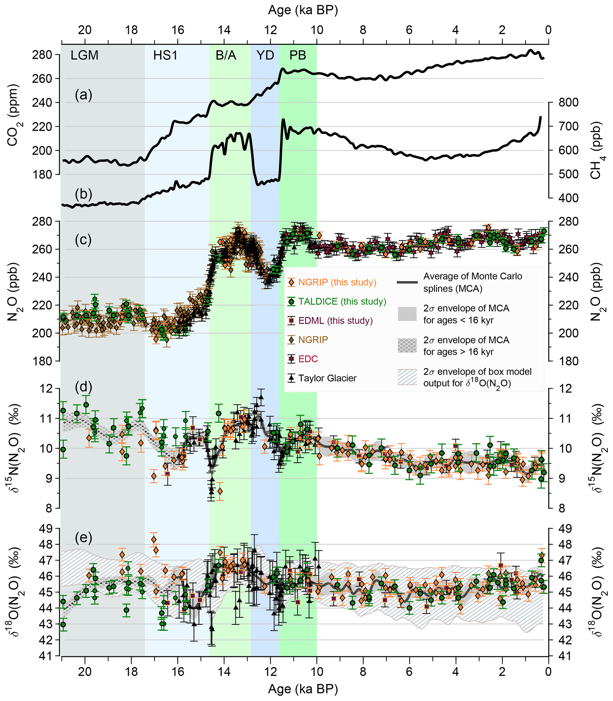
Figure 3Greenhouse gas records over the last 21 kyr after removing N2O samples affected by in situ formation. (a) CO2 concentration compilation (Bereiter et al., 2015), (b) CH4 concentration (Loulergue et al., 2008; Rhodes et al., 2015), (c) N2O concentration as compiled in this study, (d) δ15N(N2O) and (e) δ18O(N2O) from Schilt et al. (2014) and this study. The solid lines in (c)–(e) represent Monte Carlo Average smoothing splines with a cutoff period of 2000 years prior to 16 ka BP and 700 years afterwards. The grey shaded envelopes represent the Monte Carlo based uncertainties (±2σ) of the splines. The dashed envelope in panel (e) depicts the ±2σ range of the forward modeled atmospheric δ18O(N2O) signal expected from the terrestrial and marine emissions reconstructed using N2O concentrations and δ15N(N2O) (see also Fig. 7).
As none of the isotope and concentration records is continuous and as isotope measurements are only available at a lower resolution, we derived a common lower-frequency record using a spline fitting routine (Enting, 1987), which served as input into the box model inversion used to calculate emissions. As the time interval younger than 16 ka BP was better resolved than the glacial part of the record, we used a smaller cutoff period (higher frequency content) of the spline for ages <16 ka BP and a larger cutoff period for older ages. Thus, the time interval before 16 ka BP is more strongly low-pass filtered than that after 16 ka BP. To test the sensitivity of the choice of cutoff period on our emission reconstruction, we also used splines with different but constant cutoff periods throughout the record (not shown). A higher frequency content (equivalent to a cutoff period of 900 years or lower) prior to 16 ka BP leads to erroneous variations in the spline approximation that are not supported by the measured δ15N(N2O) data and consequently to erroneous variability in terrestrial and marine emissions. The same holds true for cutoff periods lower than 500 years in the time interval after 16 kyr BP. Vice versa, very long cutoff periods (longer than 900 years) in the record younger than 16 ka BP lead to a substantial underestimation of the N2O and δ15N(N2O) variability connected to the oscillations accompanying the BA warming and the YD cold swing. Accordingly, for our best reconstruction scenario we used a cutoff period of 2000 years prior to 16 ka BP and 700 years thereafter. This change in frequency content at 16 ka BP has to be taken into account when interpreting the data; however, most of the centennial to millennial N2O emission changes discussed below are found in the time interval after 16 ka BP, where a consistent cutoff period of 700 years was used.
To derive the uncertainty of the spline approximation representative for the timescale resolved by the low-pass filter, the spline fitting was repeated 1000 times using a Monte Carlo approach, where the measurements were varied randomly within their analytical uncertainties. This Monte Carlo spline and its uncertainty was then used to detect outliers affected by in situ formation as described above. The procedure was iterated until no more outliers were found and the final Monte Carlo spline was calculated using the final data set (Fig. 3).
To assess the accuracy of ice core N2O concentrations for recent times, we compare the ice core data with overlapping firn air and direct atmospheric air measurements (Fig. 4). Reconstructions from the high-accumulation Law Dome drill site offer the best connection with the current atmospheric measurements (Etheridge et al., 1988; Francey et al., 1999). The Law Dome ice core record covers the time interval from 2 ka BP to 1979 CE and air samples obtained from the firn column and the Cape Grim air archive cover 1942 CE to 2004 CE (MacFarling Meure et al., 2006) (Fig. 4). Our new measurements using NGRIP, EDML and TALDICE ice core samples and published records from EDC and EDML overlap within the two standard deviation envelope of a Monte Carlo average spline through the Law Dome and Cape Grim data with a cutoff period of 250 years (Fig. 4). Our new concentration data also generally agree with ice core data based on the Greenland NEEM ice core (Prokopiou et al., 2018), which however show negative outliers compared to our record. These are especially pronounced in NEEM ice core samples prior to 2000 BP with N2O concentrations as low as 240 ppb. Note that the data by Prokopiou et al. (2018) are based on a dry extraction technique, which does not ensure 100 % extraction efficiency. Moreover, the extraction efficiency for N2O in air bubbles, clathrates or N2O dissolved in the ice lattice may be different and could potentially be related to the low N2O concentrations in this interval. Our new compilation based on Greenland (NGRIP) and Antarctic (EDC, EDML, Talos Dome) ice cores consistently shows concentrations of 265–270 ppb in this time interval, similar to what is found during preindustrial times. In view of the good agreement of several Greenland and Antarctic ice cores and the better data resolution in our record, we decided not to use the NEEM samples by Prokopiou et al. (2018).
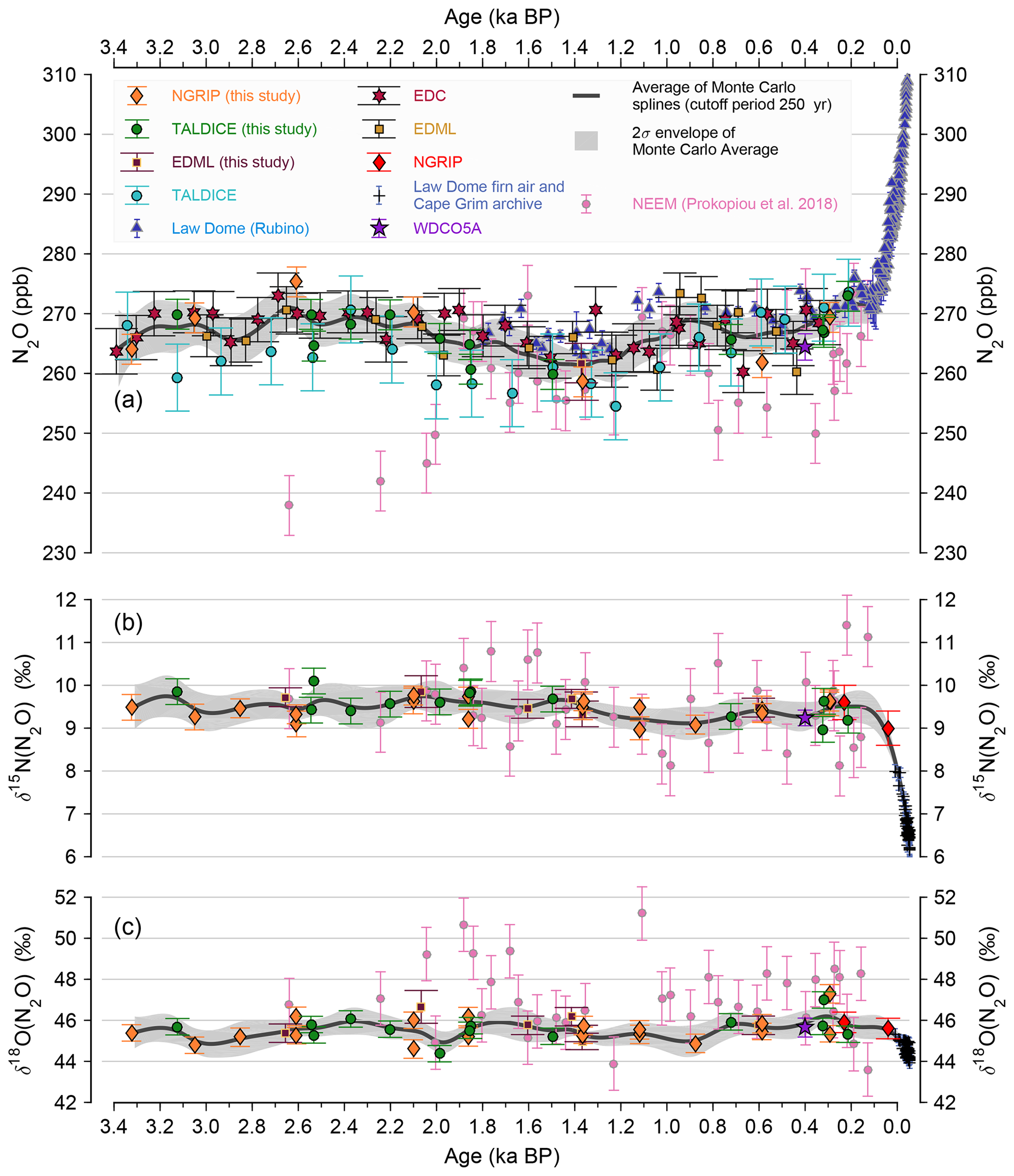
Figure 4Late Holocene evolution of (a) N2O concentrations from this study and published records (Bernard et al., 2006; Flückiger et al., 2002; MacFarling Meure et al., 2006; Park et al., 2012; Schilt et al., 2010b; Schmitt et al., 2014; Rubino et al., 2019; Prokopiou et al., 2018) (b) δ15N(N2O) and (c) δ18O(N2O) from this study and published records (Bernard et al., 2006; Park et al., 2012; Schmitt et al., 2014; Prokopiou et al., 2018), connecting the ice core records and the independent reconstructions using firn air and the Cape Grim air archive (Park et al., 2012).
In case of the N2O isotopic records very few other reconstructions are available. NGRIP results (Bernard et al., 2006) connect our youngest data points with the firn air and Cape Grim archive measurements (Fig. 4) capturing the recent anthropogenic perturbation (Park et al., 2012). The recent study by Prokopiou et al. (2018) also provides δ15N(N2O) and δ18O(N2O) data prior to the preindustrial period from the NEEM ice core (Fig. 4). Isotopic analyses in that publication also differentiate the nitrogen isotopic signature of molecules with the 15N located at the central δ15Nα(N2O) or terminal δ15Nβ(N2O) position, which we cannot distinguish by our method.
The δ15N(N2O) data from the NEEM ice core (Prokopiou et al., 2018) are in general agreement with our data set measured at the University of Bern based on Greenland (NGRIP) and Antarctic (EDML, Talos Dome) ice cores. However, our data show rather constant nitrogen isotopic signatures around +9 ‰ to +10 ‰ over the time interval 3.3–0.2 ka BP, i.e., significantly less scatter than the data by Prokopiou et al. (2018). This overall supports the conclusions drawn from the δ15N(N2O) record for the late Holocene (Prokopiou et al., 2018), but our more precise data constrain the late Holocene N2O budget and its variability much more closely. Accordingly, we refrain from using the δ15N(N2O) data by Prokopiou et al. (2018) in our model deconvolution.
Also, our δ18O(N2O) data show rather constant values in the late Holocene between +45 ‰ and +46 ‰. The values of Prokopiou et al. (2018) are higher in this time interval by +1 ‰ to up to +6 ‰ relative to our data. Such large offsets cannot be explained by differences in the isotopic standards used in the different labs. The much larger variability in the data by Prokopiou et al. (2018) connected to generally higher δ18O(N2O) compared to our data is not easy to explain. Any fractionation occurring during an (incomplete) gas extraction is expected to have an effect on δ15N(N2O) as well, which is not observed. Incomplete cryo-sampling of N2O during gas collection may explain lower N2O concentrations and higher δ18O(N2O) but again a similar effect on δ15N(N2O) would be expected. In view of the better data quality of our record we refrain from using the data by Prokopiou et al. (2018) in our δ18O(N2O) compilation. As we do not use δ18O(N2O) in our box model deconvolution to constrain terrestrial and marine emissions, the offset between the two data sets has no impact on the conclusions drawn in our study.
2.2 Reconstructing marine and terrestrial N2O emissions by deconvolving the N2O and δ15N(N2O) ice core records
2.2.1 Monte Carlo two-box model
We deconvolved the evolution of tropospheric N2O and δ15N(N2O) with a two-box atmosphere model following Schilt et al. (2014). This yields both the global terrestrial and the global marine N2O source evolution. This novel source reconstruction for the past 21 kyr permits us to disentangle various hypotheses put forward to explain the observed N2O changes. In addition, the reconstructed emission time series serve as benchmark for mechanistic and coupled climate/biogeochemical models simulating land and ocean N2O emissions.
The minimal two-box atmosphere model features a tropospheric and stratospheric box as well as a land and ocean source and includes N2O, δ15N(N2O), and δ18O(N2O) as tracers. Air exchange between the troposphere and stratosphere is assumed time-invariant and N2O is destroyed in the stratosphere assuming an e-folding lifetime and considering isotopic fractionation. N2O sources are inversely calculated by prescribing tropospheric N2O and δ15N(N2O) from the splines of the composite ice records as input data. The two budget equations for tropospheric N2O and δ15N(N2O) are solved at each time step for the two unknown global source fluxes for a given set of model parameters, initial conditions and tropospheric input data.
δ18O(N2O) serves as an independent check of consistency. To this end we used the terrestrial and marine emission records to calculate the tropospheric δ18O(N2O) signature in a forward model mode and compared it with the measured δ18O(N2O) record. The envelope of ±2 standard deviations around the mean of this Monte Carlo forward output is relatively large (Fig. 3) due to the large range of possible source signatures of terrestrial and marine sources. Nevertheless, Fig. 3 shows that our source deconvolution is in agreement with the δ18O(N2O) measurements.
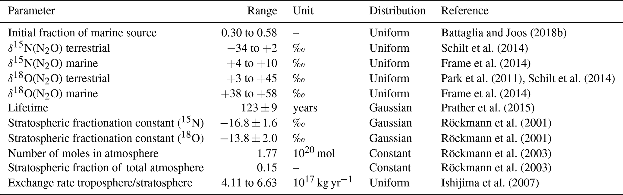
A Monte Carlo approach is used in the deconvolution to estimate uncertainties in N2O land and ocean emissions (see details in Schilt et al., 2014). Initial conditions and model parameters (Table 2) and tropospheric input data are varied randomly within their uncertainties. Model parameters are kept time invariant during a single Monte Carlo run, except in sensitivity simulations (see below). Model parameters include atmospheric lifetime, exchange rate of air between troposphere and stratosphere, stratospheric fractionation coefficients, and characteristic isotopic compositions of the terrestrial and marine sources. In particular, δ15N(N2O) is varied between −34 ‰ and +2 ‰ for the global terrestrial emissions (Schilt et al., 2014) and between +4 ‰ and +10 ‰ for global marine emissions (Frame et al., 2014). In order to constrain the model by the current knowledge of the ratio of natural marine and land emissions (Battaglia and Joos, 2018b), the allowed fraction of marine emissions to total emissions (fm) at the start of each run at 28 ka BP must lie between 30 % and 58 % close to the confidence interval for fm given by Battaglia and Joos (2018b). In principle the model could freely evolve from this starting point, but the results show (see Fig. 7 below) that fm is not varying largely over time and that the late Holocene value in our runs is very close to the best estimate of 43 % by Battaglia and Joos (2018b). For each Monte Carlo iteration the model is forced with an individual Monte Carlo realization of the splined ice core data with cutoff periods of 2000 years (28–16 ka BP) and 700 years (16–0 ka BP), where the measured values were varied within the distribution of the measurement uncertainty. Average sources and their 2σ uncertainty bands are then obtained from 500 solutions.
Table 2Parameter ranges used in the atmospheric two-box model for the calculation of terrestrial and marine N2O emissions.
2.2.2 Model performance tests and limitations
In order to test whether the model is able to reliably reconstruct terrestrial and marine emissions during rapid changes in the N2O budget using N2O concentration and δ15N(N2O) records from ice cores, we used artificial data mimicking the fast emission changes seen at the onset of the BA. These tests become especially important as the true data resolution is limited and because we use a spline approximation as input to the model. Moreover, ice core values represent a low-pass filtered version of the atmospheric record due to the slow bubble enclosure process at the firn/ice transition.
Due to the slightly different atmospheric lifetimes of 14N2O and 15N2O, significant variations in the isotopic signature of atmospheric N2O are expected over a time interval of a few centuries following a rapid increase in N2O emissions, even if the isotopic signature of the emissions remained constant. Accordingly, our transient deconvolution technique must be also able to correct for this so called “disequilibrium effect” in the low-pass filtered ice core record to derive unbiased terrestrial and marine emissions values.
We performed three test runs assuming (i) a ramp-up of land emissions only over 50 years with a constant nitrogen isotopic signature of −18 ‰, (ii) a ramp-up of marine emissions only over 50 years with a constant nitrogen isotopic signature of +7 ‰, and (iii) a proportional ramp-up of both land and marine emissions over 50 years using the constant isotope signatures given above (Fig. 5). The increase in total emissions was kept the same in all three runs. The emissions were used to drive a forward version of our model to calculate atmospheric N2O concentrations as well as its isotopic signatures. We refer to this data set further on as “artificial atmospheric data”. The emission changes led to an increase in atmospheric N2O from about 220 to 260 ppb, similar to what is observed at the BA onset (Fig. 5). The δ15N(N2O) signature of the atmosphere changed from a value of 10 ‰ before the emission change to a value of 8 ‰ in case (i), 12 ‰ in case (ii) and remained the same after fading out of the disequilibrium effect in case (iii) (Fig. 5). These atmospheric records were then low-pass filtered using a log-normal gas age distribution with a mean age of 132 years (Köhler et al., 2011) to mimic the bubble enclosure process. According to latest experimental results this represents an upper limit of the width of the age distribution in the bubbles over the deglacial for all the cores used in our compilation (Fourteau et al., 2017). Accordingly, this filter provides a conservative estimate of the maximum effect of the bubble enclosure on our deconvolution. We refer to this low-pass filtered version further on as “artificial ice core data”. The low-pass filtered atmospheric data were then used as input in our Monte Carlo box model deconvolution, where the input data from the artificial ice core data are splined with a cutoff period of 700 years. We refer to this record further on as “splined artificial ice core data”. The reconstructed emissions were compared to the input data and contrasted to the reconstructed emissions from the true ice core record at the onset of the BA. For the latter comparison we synchronized the well-defined onset of the CH4 increase in the ice core record with the start of the N2O emission increase in our test runs assuming that CH4 and N2O started to increase synchronously in response to the rapid warming events.

Figure 5Deconvolution of artificial ice core data for a hypothetical 50-year emission ramp-up of (i) terrestrial emissions, (ii) marine emissions and (iii) terrestrial and marine emissions in a fixed ratio. (a) Assumed terrestrial and/or marine emission increases for scenarios (i) to (iii). The increase in total emissions is the same in all cases; however, the contributions of terrestrial and marine sources differ in the three scenarios. fm denotes the change in the fraction of marine to total emissions during these three runs. (b) Calculated N2O concentration before (dashed black line) and after low-pass filtering with a log-normal gas age distribution with a mean gas age of 132 years mimicking the bubble enclosure process (solid black line). The dotted black line represents the artificial ice core data after applying a spline approximation with a cutoff period of 700 years. (c) Calculated δ15N(N2O) before (dashed colored lines) and after low-pass filtering (solid colored lines) with the log-normal gas age distribution and after applying a spline approximation with cutoff period of 700 years (dotted colored lines), (d) deconvolution results using the data in (b) and (c) showing terrestrial (solid colored lines) and marine (dashed colored lines) emissions. Also plotted for comparison are the reconstructed emissions using the ice core data at the onset of the BA warming (grey lines in b–d), where the ice core results are plotted on the model timescale assuming that the well-defined onset in the ice core CH4 increase (vertical blue dashed line in Fig. 2) is synchronous with the onset of the N2O emission increase in the artificial data.
The results of these performance tests are summarized in Fig. 5 with the increase in N2O emissions starting at model year 5000. As illustrated in Fig. 5, the model deconvolution is able to unambiguously separate terrestrial and marine emissions despite the low-pass filtering by the bubble enclosure process and the spline approximation and despite the disequilibrium effect. The model is able to reconstruct the total amplitude in emission fluxes well; however, the temporal resolution of fast emission changes is hampered by the low-pass filtering of the data. We also performed tests with a much larger expected value of the gas age distribution of 330 years (a typical deglacial value derived from firnification models for low accumulation sites such as EDC; Köhler et al., 2011) and our method was also able to unambiguously reconstruct the emission changes in this case (not shown).
As can be seen in Fig. 5b and c, the N2O concentrations in the artificial ice core data and its isotopic composition start to change a few decades after the onset of the true emission increase in the input data. This can be readily explained by the log-normal age distribution assumed to mimic the low-pass filter of the bubble enclosure process, which has a very long tail of air bubbles containing very old air, thus leading to a small delay in the onset of the reconstructed emission changes. This effect is more pronounced assuming a mean age of the gas age distribution of 330 years (not shown) instead of 132 years. In real ice core data this offset is compensated by a shift in the gas age scale relative to the ice age scale.
The long tail of old air in the gas age distribution together with the spline approximation is also the reason for the time needed in the emission reconstruction based on the splined artificial ice core data to reach its maximum, which takes several hundred years longer than the 50 years ramp-up in the originally assumed emission increase. Note that a log-normal age distribution is overestimating the width of the true age distribution in the ice and especially the long tail of old air is not realistic. The effect of this low-pass filtering on the synthetic data is, therefore, stronger than the effect of the true bubble enclosure in the ice and the effects illustrated in Fig. 5 can be regarded as an upper limit of the true delay and the response time. Note also that the reconstructed emission increases in Fig. 5d appear to start about 2 centuries earlier than the major increase in the input fluxes and the artificial ice core data. This lead is an artifact created by the use of the splined artificial ice core data as input to our model.
In view of the reasonable model performance described above, the comparison of the artificial data runs with the true ice core reconstructions for the BA warming in Fig. 5 suggests that for example the rapid N2O increase at the onset of the BA is mainly of terrestrial origin while the major marine emission increase is delayed to this onset by a few centuries (see results and discussion). While our transient box model deconvolution accounts for the long atmospheric lifetime of N2O, it – of course – cannot correct for the low-pass filtering of the bubble enclosure process and the spline approximation. This is the reason why the emission reconstruction takes about 350 years from the start of the emission increase in the input data (and about 550 years from the start of the first increase in the reconstructed emissions) to accomplish 90 % of the emission increase. This is very likely also the reason why the duration of the terrestrial emission increase in the ice core based reconstruction (grey line in Fig. 5) has a similar timescale, while the rapid warming in Greenland and the North Atlantic occurred only in a few decades (Erhardt et al., 2019; Steffensen et al., 2008).
In summary, our model can reliably separate terrestrial and marine emissions. The onset of rapid increases in total N2O emission can be clearly identified using the high-resolution N2O concentration record itself; however, the resolution of individual terrestrial and marine emission reconstructions is still limited by the available resolution of the δ15N(N2O) record. The precise temporal evolution of emission changes could be improved in the future if the true gas age distribution in the ice were known (Fourteau et al., 2017) and when even higher data resolution and precision become available that allow us to use input data with a higher frequency content than our spline with a cutoff period of 700 years.
2.2.3 Sensitivity runs
In two sensitivity tests, we investigated the influence of the prescribed initial range of the marine contributions to total N2O emissions and varied the initial fraction of marine emissions only between 25 % and 35 % and between 53 % and 63 % as alternatives to our standard run, where this contribution was varied over a larger range from 30 % to 58 % (Fig. 6). Sensitivity simulations were also used to probe the influence on time-varying changes in the isotopic signature of terrestrial (Amundson et al., 2003; McLauchlan et al., 2013) and marine N2O emissions (Galbraith and Kienast, 2013) and in the atmospheric lifetime (Kracher et al., 2016).
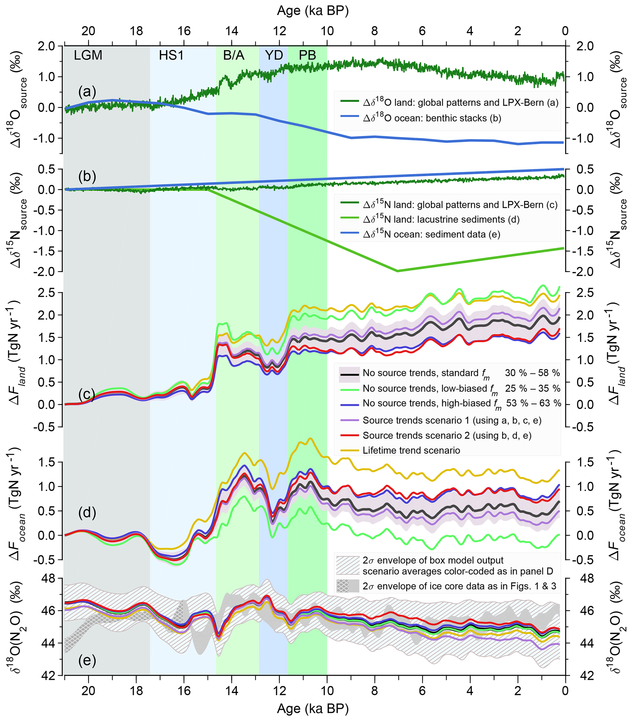
Figure 6Results from sensitivity analyses to test the robustness of N2O emissions inferred by deconvolving the ice core N2O and δ15N(N2O) records. Reconstructed, potential changes in oxygen (a) and nitrogen (b) isotopic source signatures of precursor material relative to 21 ka BP. Inferred changes in terrestrial (c) and marine (d) N2O emissions anomalies relative to 21 ka BP, (e) atmospheric δ18O(N2O) from ice cores (dark grey band) and inferred from the terrestrial and marine emissions in panels (c) and (d). Emission anomalies of the standard deconvolution in (c)–(e) are shown in black including their ±1 standard deviation uncertainty (grey shading). Sensitivity setups refer to runs with a lowered (green) and elevated (blue) marine source fraction range at the start of the runs, temporal terrestrial source signature changes derived from model data (purple line) and from lacustrine sediments (red line), and using a time-dependent atmospheric lifetime (yellow) as described in detail in Sect. 2.2.3. In both source signature scenarios (purple and red line), marine source signatures are varied according to evidence from marine sediment records.
δ15N(N2O) (as well as δ18O(N2O)) of terrestrial and marine N2O emissions are kept time-invariant in the standard deconvolution setup; however, these isotopic source signatures may have changed over time. We constructed scenarios for temporal changes in the δ15N signatures of global terrestrial and marine N2O emissions to test the sensitivity of inferred terrestrial and ocean N2O emissions to these changes in source signatures (Fig. 6). The scenarios are based on scarce, and partly conflicting, observational evidence. They are used here solely as indicative measures of the potential magnitude of plausible temporal changes in the δ15N signature of emitted N2O.
Amundson et al. (2003) provide empirical relationships between δ15N of the integrated soil N pool (0–50 cm depth), δ15Nsoil, and local annual mean temperature, MAT (in ∘C), and annual mean precipitation, MAP (in mm yr−1):
This relationship is derived from modern spatial gradients in climate and soil nitrogen isotopic signatures. Here, we transferred this relationship to estimate the potential magnitude of a temporal change in δ15N of N2O emitted from soils. The relationship was evaluated for each grid cell using transient climate data from the TraCE-21kyr model run covering the last 21 000 years (Liu et al., 2009; Otto-Bliesner et al., 2014). Global average signatures are calculated as the flux weighted mean of simulated N2O emissions in LPX-Bern (version 1.4) at decadal resolution and for the past 21 000 years (see Joos et al., 2019a, for details of the setup of LPX-Bern). Similarly, soil experiments of N2O production reveal that the difference of δ18O between soil water and produced N2O is linearly related to the water filled pore space (WFPS) and we applied the relationship given by Lewicka-Szczebak et al. (2014) using WFPS and N2O emissions as simulated by LPX-Bern (version 1.4). This yields an N2O emission-weighted, global mean change in isotopic source signature from 18 to 0 ka BP of about +0.4 ‰ for δ15N and of about +0.8 ‰ for δ18O (dark green line in Fig. 6a and b). The reliability of these estimates remains questionable, as it is, for example, not clear whether the current geographical relationship between bulk soil δ15N with climate holds also for temporal changes in δ15N of emitted N2O from soils.
δ15N data of lacustrine sediments (McLauchlan et al., 2013) suggest an opposite signal than estimated from the empirical climate-δ15N relationship. The stacked data show a 2 ‰ decrease in δ15N from 15 to 7 ka BP and an 0.6 ‰ increase thereafter (light green line in Fig. 6b). The stack of lacustrine sediments is from sites predominantly outside the main N2O emission regions (see Fig. 1 in McLauchlan et al., 2013), and may not be representative for global changes in δ15N in soils. In addition, it is plausible that with a change in soil N availability, pathways of N loss and fractionation processes relevant for N2O emissions may change as well. In brief, the δ15N trend from lacustrine sediments may not necessarily correspond to the trend in δ15N of N2O emitted from the land biosphere.
As a measure of potential changes in δ15N of marine N2O emissions, we apply reconstructed changes in δ15N of marine sediment material (blue line in Fig. 6b) which amount to about +0.4 ‰ from 18 to 0 ka BP period (Galbraith and Kienast, 2013). Further, the trend in δ18O from a global benthic isotope stack corrected for temperature changes (Elderfield et al., 2012; Lisiecki and Raymo, 2005) is applied to estimate potential temporal changes in δ18O(N2O) (blue line in Fig. 6a).
This yields two scenarios for isotopic source change. The temporal changes in δ15N of global terrestrial emissions are either prescribed according to the empirical relationship (scenario 1; purple line in Fig. 6c to e) or from changes in δ15N from stacked records of lacustrine sediments (scenario 2; red line in Fig. 6c to e). In both scenarios marine δ15N and δ18O source signatures are varied according to the evidence from marine sediment records. The resulting land and ocean N2O emissions are shown in Fig. 6c and d.
Finally, we tested the sensitivity of our box model approach to temporal changes in the atmospheric lifetime (yellow lines in Fig. 6c–e), which is controlled by the troposphere/stratosphere exchange. The Brewer–Dobson circulation and atmospheric lifetime of N2O may change over time. Kracher et al. (2016) find a linear relationship between the relative change in atmospheric lifetime of N2O and the change in global mean surface air temperature (SAT) with a slope of −5.87 % K−1 in idealized global warming simulations. Taken at face value, their results imply a longer lifetime during the LGM and a shorter lifetime in the early Holocene compared to preindustrial conditions. We applied the slope of Kracher et al. (2016) in a simulation with an idealized deglacial temperature evolution. SAT was assumed to increase linearly by 3.5 ∘C between 17 and 11 ka BP and to decrease linearly by 0.7 ∘C over the Holocene (Marcott et al., 2013; Shakun et al., 2012); the N2O lifetime was varied accordingly. Obviously, the box model does not represent the Brewer–Dobson Circulation, but summarizes troposphere-to-stratosphere exchange in a single air mass exchange parameter only. Therefore, we varied the stratospheric decomposition rate of N2O in the model to enforce changes in lifetime. The scenario yields an atmospheric lifetime that is about 16 % (20 years) higher for LGM than for preindustrial conditions. Accordingly, the inferred marine and terrestrial emissions over the past 21 kyr are about 16 % higher than in the standard deconvolution setup (Fig. 6b and c). Within the framework of our two-box model, the partitioning between marine and terrestrial emissions is not sensitive to this temporal change in lifetime.
3.1 Ice core data of N2O, δ15N(N2O) and δ18O(N2O)
Reconstructed tropospheric N2O shows an overall increase from around 210 ppb at the LGM (21 ka BP) to 270 ppb before the onset of industrialization (Fig. 3). During the late glacial, N2O concentrations alternated around a relatively constant level of around 210 ppb after declining from an elevated level of up to 240 ppb during DO event 3 at around 28.5 ka BP (see Fig. 1). Even during this late glacial interval between 26 and 18 ka BP, significant variations in N2O concentrations can be resolved with pronounced concentration minima of around 200 ppb at 25 ka BP (potentially related to Heinrich event 2), at 24.5 ka BP and less pronounced at around 23.5 ka BP.
During the deglaciation, the N2O record features a pronounced millennial-scale decrease by about 15 ppb from 17.4 to 16.6 ka in the early phase of the Heinrich Stadial 1 Northern Hemisphere (NH) cold phase (HS1; 17.4 to 14.6 ka BP; Rasmussen et al., 2014) followed by a slow recovery in the second phase of HS1. At the end of HS1 (the onset of the BA NH warm period; 14.6 to 12.8 ka BP) N2O shows a very rapid increase by almost 40 ppb, followed by a slower increase to peak values in the late BA. N2O decreased again by about 20 ppb from 13 to 12 ka BP in the early part of the YD NH cold period (YD; 12.8 to 11.7 ka BP), followed by a recovery during the late YD to reach peak values around 11 ka BP after a rapid increase at the end of the YD.
During the early Holocene N2O shows another decrease from about 270 to 260 ppb in the interval from 11 to 10 ka BP followed by rather constant mixing ratios until about 5 ka BP. After 5 ka BP N2O increases to about 270 ppb and is generally more variable than in the early Holocene. In this period, N2O varies on multi-centennial to millennial timescales between 272 and 262 ppb with maxima around 4.5 and 2.6 and minima at 3.8 and 1.4 ka BP. For the most recent millennia (Fig. 4) there exists excellent overlap of N2O data from many different ice core sites and analytical techniques and the ice core record is seamlessly linked to instrumental N2O measurements of tropospheric background air by the Law Dome data (MacFarling Meure et al., 2006). This not only provides confidence in the ice core reconstructions, but also provides a robust view on the millennial-scale N2O oscillation during the late Holocene. From the local N2O maximum with ca. 270 ppb at around 2.6 ka BP, N2O dropped by around 8 ppb to reach a minimum at 1.4 ka BP followed by a recovery within around 200 to 400 years (Fig. 4).
δ15N(N2O) varied within only about 2 ‰ over the past 28 kyr (Fig. 1). This suggests that the relative contribution of isotopically light and isotopically heavy emission sources did not change substantially. There is an overall net change in δ15N(N2O) from 21 ka BP to the preindustrial by about −1 ‰ and some small but distinct variations in the course of the last glacial termination. Prior to 22 ka BP, δ15N(N2O) data exist only from the Greenland NGRIP ice core (Fig. 1), which appears to be isotopically quite low in δ15N(N2O) for dusty glacial ice compared to the Antarctic Talos Dome (TALDICE) ice core, where data exist after 23 ka BP. As the NGRIP data proved to be more prone to in situ N2O production compared to the TALDICE core, we refrain from quantitatively interpreting the N2O isotope data prior to 21 ka BP using the box model deconvolution. During the time period from 21 ka BP to the preindustrial (Fig. 3) it is interesting to note that the minima in N2O around 17.5 ka in HS1 seems reflected by a corresponding minimum in δ15N(N2O), whereas the two other distinct minima in δ15N(N2O) at 14.6 and 11.6 ka BP coincide with the rapid N2O rise at the onset of the BA and the Preboreal NH warm phases. In the two latter cases atmospheric δ15N(N2O) is highly affected by the disequilibrium effect and a model deconvolution is required to reliably derive the dynamics in nitrous oxide source changes. The overall decrease in δ15N(N2O) by about −1 ‰ from the LGM to the preindustrial is not affected by this effect and points to an increasing share of terrestrial emissions on total emissions over the deglaciation.
δ18O(N2O) also varied modestly (typical range of 3 ‰) during the past 28 kyr around a mean value of about 45 ‰ (Fig. 1). Again, we concentrate on the interpretation of the last 21 kyr (Fig. 3) in terms of isotope changes as the δ18O(N2O) signature of the NGRIP data prior to 23 ka BP appears to be offset (by about +1 ‰) relative to the TALDICE data. The δ18O(N2O) record over the last 21 kyr suggests a minimum around 15.5 ka BP and highest values during the BA, while δ18O(N2O) varied around 45 ‰ to 46 ‰ in the Holocene and comparable to LGM values. Despite a lower signal-to-noise ratio compared to δ15N(N2O), δ18O(N2O) appears to become progressively isotopically lighter (more negative) in the first half of the Holocene and seems to increase again thereafter. Note that there is no overall correlation between the δ15N(N2O) and δ18O(N2O) records. The low correlation may be linked to overall small variability in the two records and to differences in the processes affecting δ15N(N2O) and δ18O(N2O) with δ18O also being affected by changes in the water cycle and ice sheet mass, while δ15N(N2O) being dependent on the efficiency of nitrogen turnover in soils or in low oxygen water masses of the ocean.
3.2 Reconstructed changes in terrestrial and marine N2O emissions: deconvolving the ice core N2O and δ15N(N2O) records
3.2.1 Inferred emission changes
The N2O and δ15N(N2O) records allow us to disentangle changes in global terrestrial and global marine N2O emissions to the atmosphere since the LGM. To this end we used the two-box model deconvolution of the N2O and δ15N(N2O) records described in Sect. 2.2 to determine marine and terrestrial N2O emissions and their uncertainty (Fig. 7) over the last 21 kyr. The uncertainty (colored shading in Fig. 7) of the absolute emissions (left y axes) is relatively large, reflecting the large range of possible isotopic source signatures for marine and terrestrial emissions accepted in the box model runs, which spreads essentially over the entire allowed range of terrestrial and marine source signatures. Together with the constraint on the marine emission fraction, this determines the absolute level of terrestrial and marine emissions in each of our accepted Monte Carlo runs (see Fig. 7 for three examples of individual runs (grey lines)). Note that these individual runs are systematically offset from each other dependent on the choice of the isotopic source signature, but that the anomalies relative to the LGM level of all runs are very similar. Thus, using our Monte Carlo box model deconvolution with randomly chosen but temporal constant isotopic source signatures, we can quantify emission anomalies relative to the LGM level much more precisely than the absolute emission level using or deconvolution.

Figure 7Reconstructed global terrestrial (a) and marine (b) N2O emission changes: mean reconstructed terrestrial and marine N2O emissions are shown by the solid green and blue lines, respectively, together with their uncertainty estimate (±1σ; colored shaded area) based on 500 accepted runs calculated using the Monte Carlo atmospheric two-box model (Schilt et al., 2014) and ice records of N2O concentration and δ15N(N2O). (c) mean reconstructed marine fraction fm of total emissions (solid brown line) and its 1σ uncertainty (orange shaded area). y axes on the left indicate reconstructed absolute emissions, y axes on the right indicate the terrestrial and marine emission anomalies relative to the LGM (21 ka BP). The dashed colored lines around the mean anomalies indicate the ±1σ uncertainty of the reconstructed anomalies. Note that the uncertainties of the anomalies are smaller than those of the total fluxes, as the choice of the isotopic source signatures in the Monte Carlo approach systematically shifts total emission fluxes in an individual run to higher or lower values but not the anomalies. This is illustrated by three randomly selected runs (runs 1, 2, and 3, indicated by grey lines), which are systematically offset from each other in (a)–(c). In summary, we are able to reconstruct anomalies in the N2O emissions relative to the LGM more precisely than the overall level of marine and terrestrial emissions using our approach.
Reconstructed terrestrial and marine N2O emissions increased between the LGM (21 ka BP) and full interglacial conditions (7 ka BP) by 1.5±0.3 and 0.5±0.3 TgN yr−1 (mean ± 1 standard deviation) and between LGM and PI conditions (1500 CE) by 1.7±0.3 and 0.7±0.3 TgN yr1, respectively. Marine sources first dropped by ∼0.5 TgN yr−1 during the onset of HS1, when AMOC strongly decreased (McManus et al., 2004). This drop into HS1 also explains the apparently higher marine emission change estimate in Schilt et al. (2014), who, due to the limited data availability at that time, provided an emission anomaly relative to the value at 16 kyr instead of 21 kyr BP. Marine emissions remained minimal over the following millennium, but started to increase around 16 ka BP and recovered to LGM levels around 15 ka BP in the course of HS1, while AMOC remained constantly low (McManus et al., 2004). This pattern of recovery during cold stadials has been observed before (Schilt et al., 2013) and is tentatively attributed to a slow recovery of N2O production in subsurface waters as also suggested by marine nitrogen cycle modeling (Schmittner and Galbraith, 2008; Joos et al., 2019b). Our quantitative emission reconstruction shows for the first time the complete evolution of marine (and terrestrial) N2O emissions over the entire HS1 interval. The isotope results demonstrate that the millennial decrease at the beginning of HS1 and the later increase in atmospheric N2O during HS1 are indeed caused by marine emissions and may be linked to the substantial ocean reorganization that is thought to have determined the early deglacial rise in atmospheric CO2 (Schmitt et al., 2012; Tschumi et al., 2011; Jaccard et al., 2016). In contrast, terrestrial N2O emissions remained approximately invariant until the start of the BA warm period in the Northern Hemisphere. Then, land emissions rapidly increased at the start of the BA, declined again during the YD, and peaked again after a rapid rise into the Preboral, consistent with earlier results for the 16 to 10 ka BP interval (Schilt et al., 2014). Also marine emissions generally start to increase during the BA warming, however, not as rapidly as terrestrial emissions, and the main marine increase is delayed by a few hundred years relative to the onset of the rapid atmospheric N2O concentration increase. A similar pattern is found for the rapid warming at the end of the YD. Note also that while terrestrial emissions remained relatively low over the entire course of the YD, marine emissions show a slow recovery that starts about 1000 years before the rapid N2O increase at the end of the YD into the Preboreal.
Compared to the drastic emission changes over the deglaciation, the trends in terrestrial N2O emissions are comparably small during the Holocene. Our deconvolution suggests only a very small increase in terrestrial emissions over the first half of the Holocene. Consistently, the decline in atmospheric N2O concentrations in the early Holocene is attributed to a reduction in marine emissions. The 10 ppb higher N2O concentrations in the later Holocene are mainly attributed to an increase in terrestrial emissions which occurred predominantly in the time interval from about 6.5 to 5 ka BP. Marine emissions show only slightly increased values after 6 ka BP interrupted by a weak decline in marine emissions in the time interval 2.5–0.5 ka BP (Fig. 7). However, the uncertainty in our reconstructed emission anomalies based on N2O and δ15N(N2O) during the Holocene is as large as the reconstructed emission changes (Fig. 7, solid and grey dashed lines), leaving some doubt about the significance of this reconstructed ocean emission anomaly. Looking at the δ18O(N2O) record in Fig. 3, which was not used in the deconvolution, δ18O(N2O) values are about 1 ‰ higher after 2.5 ka BP than before which – taken at face value – would contradict reduced N2O emissions by marine sources. A similar caveat applies to the millennial variability in marine and terrestrial emission over the Holocene. The well-resolved and precise reconstruction of atmospheric N2O concentrations (Fig. 3) shows significant maxima around 4.5 and 2.5 ka BP and less pronounced maxima around 9.0, 7.3 and at 5.8 ka BP as well as minima at 8.3, 6.5, 3.6 and 1.4 ka BP, documenting significant millennial changes in total N2O emissions. However, the nitrogen isotope-based reconstruction of terrestrial and marine emissions does not yet allow for an unambiguous attribution of these changes to one source category. It may be tempting to attribute these millennial N2O emission changes over the Holocene to changes in the AMOC strength or variations in the position of the ITCZ and the monsoonal rain belt (for example for the 8.2 ka cold event in Greenland; Spahni et al., 2003) or to apparent large-scale climate changes in the course of the Holocene (Wanner et al., 2011). However, no consistent connection of N2O emission maxima or minima with global climate changes can be recognized and no quantitative attribution to terrestrial or marine sources is possible at this point. To this end, higher-resolution isotope records and further improvements in precision of the δ15N(N2O) analyses will be necessary to better constrain small changes in the N2O budget over the Holocene.
Our new ice core isotope data permit novel insights in the response timescales of terrestrial and marine N2O emissions during periods of rapid climate change. Using our box model deconvolution approach, we can in principle resolve rapid emission changes which are otherwise hidden in the atmospheric N2O concentration record by the relatively long atmospheric lifetime (see methods). However, the ice core record presents a low-pass filtered version of the atmospheric changes due to the bubble enclosure process, which generally leads also to a documented response in the ice core record which is delayed and smoothed relative to the atmosphere. Moreover, as input data for the deconvolution we use the Monte Carlo spline estimate of the N2O and δ15N(N2O) records, which adds additional low-pass filtering to the ice core record. As outlined in Sect. 2.2.2, the latter leads to an erroneously early response in the emission reconstruction for rapid N2O changes. In line, the change point marking the increase in reconstructed terrestrial and marine emissions at the onset of the BA warming appears to occur earlier than the rapid CH4 increase marking the rapid warming in the gas archive, but this lead is essentially an artifact imposed by the spline filtered data used for the deconvolution and is not supported by the unsmoothed N2O concentration record. In order to pinpoint the onset of rapid changes in total N2O emissions more exactly, the higher-resolution concentration record from the NGRIP ice core (Schilt et al., 2013), where the bubble enclosure process leads to an effective resolution on the order of a few decades for the Holocene and less than a century for the Last Glacial Maximum (Schilt et al., 2013), may be used. Taking the NGRIP data after outlier removal (Schilt et al., 2013) at face value (see the discussion on potential in situ production above), this record suggests that N2O concentrations, and thus total N2O emissions, started to change synchronously within the data resolution with the CH4 concentration measured on the same samples (Fig. 2). In particular, the NGRIP N2O record excludes any significant N2O emission increase prior to the onset of the CH4 rise, where the latter is also synchronous within a few decades with the rapid warming in Greenland temperatures, as evidenced in the thermal diffusion signal in δ15N2 in the NGRIP ice core (Baumgartner et al., 2014).
The low-pass filtering also leads to an underestimation of the true atmospheric dynamics in N2O concentration changes. Using our Monte Carlo N2O concentration record compiled from all ice cores (Fig. 2), we see that 90 % of the concentration increase at the end of HS1 is achieved over a timescale of about 500 years. Using artificial emission data in forward box model runs and low-pass filtering the calculated atmospheric concentrations with a log normal age distribution with a mean age of 132 years (as applicable for the atmospheric record compiled from all our ice cores), this timescale can be achieved by a linear increase in terrestrial emission within about 200 years. In contrast, an emission increase over 300 years already requires an increase in the (bubble low-pass filtered) ice core record over 600 years. As our ice core N2O compilation is also low-pass filtered by the applied spline approximation, the true increase in the ice core concentration record should be even faster than 500 years, implying that the terrestrial emission increase happened within less than 200 years. However, based on the resolution of the available records to date we cannot constrain the timescale of the N2O emission increase to better than 200 years. In particular, we refrain from using the NGRIP concentration data, which show a more rapid increase in N2O (Fig. 2) at the onset of the BA and the end of the YD, to constrain this timescale, as these data appear to be affected by in situ formation of N2O in the ice in the respective time intervals (see discussion above).
A similar picture in terms of the timing of the onset and timescale of N2O increase as at the onset of the BA emerges for terrestrial emissions accompanying the warming at the end of the YD. Again, the major N2O concentration rise in our data compilation starts synchronously within uncertainty with CH4 and the warming in Greenland, while peak N2O concentrations are delayed by a few centuries relative to the CH4 maximum and the temperature change documented in Greenland climate records (Steffensen et al., 2008). Accordingly, this time evolution of terrestrial N2O emission changes appears to be a common feature of rapid climate changes during the last termination and potentially also for all DO events. Due to the preceding long-term increase in marine N2O emissions over the YD event, a clear acceleration of the increase in marine N2O emissions (as found for the BA warming) is difficult to discern during the rapid warming at the end of the YD. A major increase in marine emissions, however, is reconstructed at around 11.4 ka BP, which is delayed relative to the onset of the YD-Preboreal warming and lasts for about 200 years.
In summary, the terrestrial N2O emission increases at the beginning of the BA period and the end of the YD were realized within 200 years. A more rapid, decadal-scale increase in terrestrial N2O emissions is possible, but cannot be confirmed by the available ice core information to date. In any case, the terrestrial emissions increased much more rapidly than marine emissions during rapid climate warming, indicating a longer response time of the ocean compared to the land biosphere, as also suggested in a marine N2O modeling study (Goldstein et al., 2003). Modeling studies also suggest that the main response of marine N2O production and emissions is delayed by a few centuries relative to AMOC changes in idealized freshwater hosing experiments and even a longer delay is simulated until marine emission changes have reached their full amplitude (Schmittner and Galbraith, 2008; Joos et al., 2019b).
3.2.2 Testing the robustness of the deconvolution results
δ18O(N2O) was not used as additional constraint in the deconvolution but was used as independent check in forward modeling of the atmospheric concentrations and isotopic signature from the reconstructed emissions (Fig. 3). The mean results of this forward modeling suggest little change in tropospheric δ18O(N2O) in agreement with the ice core δ18O(N2O). Yet, the uncertainty range in projected δ18O(N2O) is with about ±1.5 ‰ about two times larger than the analytical uncertainty of an individual δ18O(N2O) ice core measurement (Fig. 3). This is due to the relatively wide range of possible input data (mainly the isotopic source signatures) used in our Monte Carlo box model approach. The large model uncertainty in addition to the complex nature of the global cycle of δ18O, prevents any firm conclusions from δ18O(N2O) data.
We further test the robustness of the Monte Carlo deconvolution approach to infer changes in global N2O emissions using sensitivity analyses (see Fig. 6). The results suggest a moderate sensitivity of inferred land and ocean N2O emissions to plausible changes in the global mean δ15N of N2O emissions from land and from the ocean but still well within the overall uncertainty ranges obtained from the Monte Carlo procedure. In other words, the sensitivity of inferred N2O emissions to plausible changes in δ15N of the global land and ocean emissions is smaller than the reconstructed glacial–interglacial and rapid changes. In particular, a large deglacial decrease in the land isotopic signature by 2 ‰ as suggested by lacustrine data (McLauchlan et al., 2013), requires a reduction in land emission change relative to the LGM value by only about 0.4 TgN yr−1 compared to our standard scenario (and an equivalent increase in marine emissions), i.e., very close to the 1σ uncertainty of our standard runs. Moreover, while the total glacial–interglacial increase may change (in opposite directions for marine and terrestrial emissions), the relative millennial variability seen in our records is not affected by these source scenarios.
Second, the influence of the prior assumption on the initial fraction of marine emissions relative to total N2O emissions is investigated. In the standard Monte Carlo setup, the marine contribution at the start of the deconvolution is uniformly varied between 30 % and 58 % of total emissions (equivalent to a range of 3.3 to 6.6 TgN yr−1 in preindustrial marine N2O emissions), following the most recent observation-constrained estimate (Battaglia and Joos, 2018b) with a best-guess estimate of 43 % very close to the mean preindustrial value in our reconstruction (Fig. 7). In two sensitivity tests, we investigate the influence of the prescribed initial range and vary the initial fraction of marine emissions between 25 % and 35 % (low-biased scenario, green line in Fig. 6c to e) and between 53 % and 63 % (high-biased scenario, blue line in Fig. 6c to e) only. Assuming such strong deviations from the best estimate for the marine fraction, the Holocene emission anomalies relative to the LGM level are shifted by about +1σ of the standard runs towards higher marine emissions in the high-biased scenario and by −2σ of the standards runs towards lower marine emissions in the low-biased scenario. In fact, the latter sensitivity run does show only a very small change in marine emissions between the LGM and the late Holocene. However, while a low marine fraction during the LGM as required in this run is possible, the preindustrial marine fraction in this run is lower than the best-guess estimate by Battaglia and Joos (2018b); thus, this run is likely underestimating the Holocene increase in marine emissions. To reconcile the required increase in marine fraction from the LGM to the late Holocene and our isotopic constraints asks for a significant shift in the isotopic source signatures, similar to what is observed in source signature scenario 1. We conclude that the results of our sensitivity studies overall support the robustness of our results and that the standard deviation of the emission anomalies relative to the LGM level in the standard runs provides a representative uncertainty estimate for possible emission changes. While we stress that the absolute magnitude of land and ocean N2O emissions is sensitive to selected isotopic source signature and the assumed split between marine and terrestrial N2O emissions, the relative changes in the temporal evolution of marine and terrestrial emissions are much less affected by this choice.
Finally, we varied the atmospheric lifetime over the deglacial period in an idealized scenario assuming an overall decrease in lifetime from 143 to 123 years from the glacial to the Holocene. This change in lifetime causes a parallel increase in both land and ocean emissions by about 16 %. Late Holocene emission anomalies relative to 21 ka BP increase by about 0.6 Tg yr−1 for both terrestrial and marine emissions. Again, the assumed scenario for past lifetime changes alters the absolute amplitude of emission anomalies relative to the LGM but has little effect on the temporal evolution of the emissions.
In conclusion, the main features of our standard reconstruction such as the decrease in and recovery of global marine N2O emissions during the HS1 and YD intervals and the rapid rise in global terrestrial emissions at the onset of the BA and the end of the YD are robust. The reconstructed emission anomalies relative to the LGM level clearly exceed the uncertainty ranges revealed by our Monte Carlo analysis, where both parameters and ice core data were varied within their uncertainties. The rather constant terrestrial N2O emissions in the Holocene and the slow decline in marine emissions after the Preboreal appear to be robust as well as the finding of constant terrestrial emissions during the LGM and HS1 and the overall deglacial increase in both global marine and global terrestrial N2O emissions to the atmosphere.
4.1 Reconstructed N2O emission changes
We followed the approach by Schilt et al. (2014) and deconvolved the ice core records of N2O and δ15N(N2O) to quantify changes in terrestrial and marine N2O emissions. These emission records serve as benchmarks for ocean and land models simulating N2O emissions to the atmosphere. The total emission changes are only a function of atmospheric lifetime changes; however, the split of total emissions in marine versus terrestrial emissions depends on isotopic source signatures and the assumed initial ratio of land versus ocean emissions. However within reasonable bounds of the marine emission fraction, the changes in land and ocean emission relative to the LGM level represent a robust feature of our box model deconvolution.
The temporal resolution of reconstructed N2O atmospheric concentration and marine and terrestrial emission changes is limited by the smoothing properties of the ice archive. Specifically, the transfer of atmospheric air to the firn layer and the enclosure of firn air into the ice leads to an age distribution of the air conserved in the ice and finally measured. This enclosure process acts like an asymmetric low-pass filter with a strong bias to old ages of the air enclosed, removing fast variations in N2O and N2O isotopes. In addition, for our deconvolution the ice core measurements are smoothed with a spline that acts like a (symmetric) low-pass filter to produce a continuous record from the large but limited number of samples and to account for the small but noticeable scatter in the ice core data due to measurement and archive uncertainties. Taken together, these limitations restrict the temporal resolution of changes that can be unveiled by our deconvolution. Nevertheless, we can firmly state that the terrestrial N2O emission changes at the onset of the BA and the end of the Younger Dryas started synchronously with the increase in CH4 and occurred within 2 centuries at maximum, but potentially even faster.
4.2 Marine N2O emission changes
Marine N2O emissions are controlled by the amount of organic matter re-mineralized and oxygen (O2) concentrations (Suntharalingam and Sarmiento, 2000; Battaglia and Joos, 2018b). N2O production by nitrification increases with substrate availability and with decreasing O2 concentration. The overall increase in marine N2O emission over the termination is as such consistent with paleoceanographic evidence showing an oxygen depletion across the deglaciation in the upper ocean (Jaccard and Galbraith, 2012; Moffitt et al., 2015), whereas changes in organic matter export as inferred from ocean sediments varied regionally (Kohfeld et al., 2005) and overall organic matter preservation was much higher during the LGM than the Holocene at low and mid latitudes (Cartapanis et al., 2016). The largest volumetric expansion of oxygen-depleted water masses is reconstructed for the onset of the BA, when oxygen concentrations decreased throughout the Indo-Pacific above 2500 m (Jaccard et al., 2014) and oxygen minimum zones expanded worldwide (Moffitt et al., 2015). High-resolution records from the North Pacific clearly show that hypoxic events occurred in response to the fast warming into the BA and at the end of the YD and were connected to local productivity feedbacks (Praetorius et al., 2015). In summary, upper ocean oxygen depletion appears to be the most likely explanation for the marine N2O emission increase from 16 to 13.5 ka BP, perhaps partly counteracted by a potential decrease in organic matter export and remineralization.
Marine N2O emissions show a very sharp drop around 17.4 ka BP at the onset of the HS1 and reduced emissions for the next ∼1500 years. This decreased N2O emission occurred together with the onset of the deglacial CO2 rise (Monnin et al., 2001; Marcott et al., 2014) and a concomitant equally sharp decrease in δ13C(CO2) (Schmitt et al., 2012), an increase in the deposition of biogenic opal in Southern Ocean sediments indicative of Southern Ocean upwelling (Anderson et al., 2009), a drop in atmospheric Δ14C (Southon et al., 2012; Reimer et al., 2013), and an increase in Southern Ocean oxygenation (Jaccard et al., 2016), as well as the occurrence of ice-rafted debris in Iberian Margin sediments (Bard et al., 2000). Apart from the ice-rafted debris, these changes have been explained by an intensification of Southern Ocean upwelling bringing carbon- and silica-rich and δ13C- and Δ14C-depleted waters from the deep ocean to the surface (Schmitt et al., 2012), and are consistent with the multi-tracer relationships found in dynamic ocean-biogeochemistry model simulations (Tschumi et al., 2011). Accordingly, the drop in marine N2O emissions at the onset and the low emissions during parts of the HS1 may be linked to an increase in Southern Ocean ventilation and ocean oxygen concentration during the first part of HS1.
Interestingly, both reconstructed marine N2O emissions and atmospheric CO2 show a trend change within HS1. Marine N2O emissions remained minimal within the interval from about 17.4 to 16 ka BP, while atmospheric CO2 increased by about 30 ppm during this period. Around 16 ka BP, marine N2O emissions started to rise and the growth trend in atmospheric CO2 declined. At the same time a minimum in δ13C(CO2) was reached and followed by a small increase (Schmitt et al., 2012). The change in N2O emissions and the trend reversal in δ13C(CO2) may point to a change in the mechanisms governing the rise in atmospheric CO2 which, in turn, led to a slower CO2 growth rate. This is consistent with the suggestion that Southern Ocean ventilation changes were mainly responsible for the early CO2 rise (Tschumi et al., 2011).
Paleo N2O modeling studies are sparse, but three studies present partly conflicting results for YD-type climatic events. All the studies report results from dynamic ocean models forced with freshwater hosing in the North Atlantic to provoke a collapse of the Atlantic Meridional Overturning Circulation and cooling in the North Atlantic realm. In a zonally averaged ocean model, Goldstein et al. (2003) simulated reduced marine emissions in response to reduced Atlantic overturning and a respective increase during AMOC resumption. This effect can explain about half of the reconstructed atmospheric N2O decrease/increase during the AMOC collapse/resumption. These authors proposed that terrestrial N2O emission changes must be responsible for the remaining atmospheric N2O variation and, in particular, caused the rapid increase in atmospheric N2O at the end of the YD. A recent nitrogen cycle ocean model study by Joos et al. (2019b) also shows a reduction/increase in marine N2O emissions of only 0.8 TgN yr−1, during AMOC collapse/resumption, which is not sufficient to explain the full amplitude of atmospheric N2O changes observed in the ice core record. In contrast, in the ocean model by Schmittner and Galbraith (2008) the variation in marine productivity is able to explain the full N2O concentration change observed in ice cores in response to AMOC variations. Our novel quantitative emission reconstructions support the findings by Goldstein et al. (2003) and Joos et al. (2019b). The reconstructions indeed show a slower recovery of marine N2O emissions and a much faster increase in terrestrial emissions towards the end of the YD, a N2O emission scenario already suggested by Schilt et al. (2010b).
While the centennial- to millennial-scale oscillations in terrestrial and marine emissions over the Holocene cannot be interpreted with certainty due to the still limited sampling resolution and precision of the Holocene δ15N(N2O) data, the longer-term decrease in the marine emissions over the first half of the Holocene appears significant and synchronous with a reconstructed slow increase in AMOC and subsurface water ventilation in the Atlantic Ocean (McManus et al., 2004; Waelbroeck et al., 2018) and a change in Southern Ocean bottom water properties (Jaccard et al., 2016). Thus, the processes invoked during the AMOC resumption at the end of HS1 and the end of the YD leading to a century-scale increase in marine N2O emissions cannot explain the early Holocene decrease in ocean sources. Moffitt et al. (2015) (their Table 5) show that oxic conditions expanded between 10 and 4 ka BP in the Pacific eastern upwelling systems. The extent of oxygen minimum zones in the Arabian Sea decreased from the early Holocene to mid-Holocene as ventilation of these water masses increased (Kessarkar et al., 2018). This has been related to an intensified winter monsoon and winter mixing arising from cooling in the North Atlantic region (Reichart et al., 1998). We speculate that the gradual AMOC intensification (McManus et al., 2004), accompanying the demise of the Northern Hemisphere ice sheets at a time when interglacial temperatures and sea ice extent were already established, led to an improvement in oxygenation in the low-latitude thermocline of the Atlantic and, in concert with orbital forcing and monsoonal wind changes, in the Pacific and Indian upwelling systems that may have led to the reconstructed decrease in marine N2O emissions over the first half of the Holocene.
Generally, the difference in the timescales associated with the reconstructed marine and terrestrial emission changes during the YD and over the entire termination is consistent with the notion that terrestrial N2O emissions can react quickly to climate change. In contrast, marine emission changes materialize on longer centennial to up to millennial timescales associated with surface-to-deep tracer transport and with physical and biogeochemical adjustment processes, such as changes in ocean circulation, export productivity, oxygen concentrations and the marine N2O inventory, as also indicated by multi-millennial global warming projections of marine oxygen and N2O (Battaglia and Joos, 2018a).
4.3 Terrestrial N2O emission changes
Terrestrial emissions show a 40 % increase from the Last Glacial Maximum to the late Holocene period. Most of the deglacial increase was realized in two fast and large steps. These occurred at the onset of the BA and at the end of the YD, when reconstructed terrestrial N2O emissions changed by about 1 TgN yr−1. These large changes were realized within a period of 2 centuries, and possibly faster, considering the low-pass-filtering effects of the ice archive and in the input data used for the deconvolution. The BA onset and the end of the YD are linked to rapid, decadal-scale, and widespread Northern Hemisphere warming, to shifts in the Intertropical Convergence Zone (ITCZ) and precipitation patterns, and to fast changes in atmospheric CH4 (Baumgartner et al., 2014; Rhodes et al., 2015). The latter are indicative of terrestrial methane emissions (Bock et al., 2017; Spahni et al., 2011) mainly in the tropics.
Reconstructed terrestrial N2O emissions changed relatively little during the Holocene. This is in contrast to the large reconstructed changes in land biosphere carbon stocks and in atmospheric CO2 and CH4 (Elsig et al., 2009; Flückiger et al., 2002). Ice core data of CO2 and δ13C(CO2) imply an increase in terrestrial C storage of 290±36 PgC during the early Holocene until about 6.5 ka BP, followed by a smaller release thereafter (Elsig et al., 2009). At the same time our terrestrial N2O emission reconstruction suggests only a minor increase from 11 until 6.5 ka BP, a modest increase in terrestrial emissions of up to 0.2 TgN yr−1 from 6.5 to 5 ka BP, and a rather constant overall level thereafter. The significant increase in carbon storage in the early Holocene suggests that N supply was more than sufficient to support both generally high N2O emissions and an increase in the carbon inventory in boreal peatlands (Yu et al., 2010) and possibly other regions (Stocker et al., 2017).
The apparent decoupling of significant net terrestrial carbon storage from N2O emissions in the early Holocene and an increase in N2O emissions from 6.5 to 5 ka BP, when CO2 concentrations stayed relatively constant, imply that a linear relationship between terrestrial net carbon storage and N2O production is not an adequate picture for relative changes in nitrogen turnover in soils. While it is not possible to pinpoint the responsible regional terrestrial N2O sources from the globally integrated information stored in atmospheric N2O and δ15N(N2O) in ice cores, it is worth noting that the time interval from 11 to 6.5 ka BP was characterized by a significant decrease in sea level rise rates (Lambeck et al., 2014), the disappearance of the remnants of glacial Northern Hemisphere ice sheets, and therefore most likely increased soil formation at high northern latitudes. Moreover, the Holocene was characterized by a strong decline in NH summer insolation starting around 7 ka BP and continuing over the entire Holocene with significant impacts on the position of the ITCZ and monsoonal precipitation (Wang et al., 2005; Marcott et al., 2013); however, globally integrated terrestrial N2O emissions stayed relatively constant after 5 ka BP. Thus, global nitrogen turnover in soils and the connected N2O production cannot be attributed to a controlling single factor (such as precipitation changes) or a specific region of the globe, but most likely average over competing changes in different regions throughout the globe (see also Joos et al., 2019a, for a detailed terrestrial model study of the controlling processes and the contributing source areas).
We reconstructed the evolution of the stable isotopes δ15N and δ18O of N2O for the last 28 000 years. Our N2O concentration record is seamlessly linked with the Law Dome ice and firn N2O data and with instrumental N2O measurements of tropospheric background air (MacFarling Meure et al., 2006). The age scales of the records are aligned with the absolutely counted GICC05 age scale (Rasmussen et al., 2006) using high-resolution methane measurements from Antarctica and Greenland. This leads to particularly small age-scale uncertainties around periods of rapid climate and methane changes, namely, the onset of the BA (14.6 to 12.8 ka BP) Northern Hemisphere warm period and the beginning and end of the YD (12.8 to 11.7 ka BP) Northern Hemisphere cold period.
For the last 21 000 years, where (isotopic) N2O ice core data are available at sufficient resolution and from several ice cores from both polar regions, the N2O concentration and δ15N(N2O) records allow for a quantitative reconstruction of terrestrial and marine N2O emissions. These provide important benchmarks for fully coupled, N2O and isotope-enabled Earth system models (ESMs). Particularly interesting features to investigate are the N2O depression during Heinrich Stadial I (HS1; 17.4 to 14.6 ka BP), the rapid increase in N2O to preindustrial levels at the onset of the BA and the YD fluctuation, as well as the Holocene evolution of terrestrial and marine N2O emissions.
Our records show that both terrestrial and marine N2O emissions took part in the rapid N2O increases during rapid deglacial warmings connected to the resumption of the AMOC as already shown earlier (Schilt et al., 2014). For the first time we are able to show that this is also true for the general glacial–interglacial N2O increase, while some decoupling is suggested for long-term terrestrial and marine emission trends during the Holocene. In particular, the strong deglacial increase in terrestrial N2O emissions, indicative of an enhanced nitrogen turnover in soils, implies that either nitrogen availability was not a limiting factor of vegetation growth on the longer timescales or that the relative amount of N2O produced and lost to the atmosphere during nitrogen turnover in soils increased for warmer climate conditions (Joos et al., 2019a). Reconstructed terrestrial N2O emissions changed by up to 1 TgN yr−1 and within less than 2 centuries at the onset of the NH warming events around 14.6 and 11.7 ka BP, while marine emissions changed more sluggishly to ocean reorganizations accompanying the rapid warming events during the deglacial. These timescales are also relevant for 21st century climate projections and much longer than accessible in typical laboratory or field experiments. Taken at face value, our results suggest that the terrestrial nitrogen cycle will also rapidly adjust on the global scale in the coming decades, leading to enhanced N2O emissions, while marine N2O feedbacks to future global warming induced changes in AMOC will only fully unfold on timescales of centuries in the future.
Data presented in this study will be available on the NOAA paleoclimate database.
The concept of the study was developed by HF, JS, RS, FJ, AS and EJB. Analytical methods for N2O isotopic ice core analyses were developed by JS, MB, BS, HF, AS and EJB. Ice core analyses were carried out by JS, MB, BS and AS. Deconvolution has been carried out by JS, FJ, RS and AS based on the method developed by AS. Targeted model experiments were performed by SL and GB. The manuscript was written by HF with support by JS, FJ, and RS. All the coauthors contributed to the discussion of the data and of the manuscript.
The authors declare that they have no conflict of interest.
Long-term financial support of this research by the Swiss National Science Foundation (grant no. 200020_172506 and 200020_172476) is gratefully acknowledged. Part of the research leading to these results has received funding from the European Research Council under the European Union's Seventh Framework Programme (FP/2007-2013)/ERC Advanced Grant Agreement no. 226172 (MATRICs) awarded to HF. This work is also a contribution to the European Project for Ice Coring in Antarctica (EPICA), the Talos Dome Ice Core Project (TALDICE), and the North Greenland Ice Core Project (NGRIP). EPICA is a joint European Science Foundation/European Commission (EC) scientific program, funded by the EC and by national contributions from Belgium, Denmark, France, Germany, Italy, the Netherlands, Norway, Sweden, Switzerland, and the UK. The main logistic support was provided by IPEV and PNRA (at Dome C) and AWI (at Dronning Maud Land). TALDICE is a joint European program led by Italy and is funded by national contributions from Italy, France, Germany, Switzerland, and the United Kingdom. The main logistical support was provided by PNRA at Talos Dome. NGRIP is directed and organized by the Department of Geophysics at the Niels Bohr Institute for Astronomy, Physics and Geophysics, University of Copenhagen. It is supported by funding agencies in Denmark, Belgium, France, Germany, Iceland, Japan, Sweden, Switzerland, and the USA. This is EPICA publication no. 312 and TALDICE publication no. 57.
This research has been supported by the Swiss National Science Foundation (grant nos. 200020_172506 and 200020_172476).
This paper was edited by Sönke Zaehle and reviewed by two anonymous referees.
Amundson, R., Austin, A. T., Schuur, E. A. G., Yoo, K., Matzek, V., Kendall, C., Uebersax, A., Brenner, D., and Baisden, W. T.: Global patterns of the isotopic composition of soil and plant nitrogen, Global Biogeochem. Cy., 17, 1031, https://doi.org/10.1029/2002GB001903, 2003.
Anderson, R. F., Ali, S., Bradtmiller, L. I., Nielsen, S. H. H., Fleisher, M. Q., Anderson, B. E., and Burckle, L. H.: Wind-driven upwelling in the Southern Ocean and the deglacial rise in atmospheric CO2, Science, 323, 1443–1448, 2009.
Bard, E., Rostek, F., Turon, J.-L., and Gendreau, S.: Hydrological Impact of Heinrich Events in the Subtropical Northeast Atlantic, Science, 289, 1321–1324, 2000.
Battaglia, G. and Joos, F.: Hazards of decreasing marine oxygen: the near-term and millennial-scale benefits of meeting the Paris climate targets, Earth Syst. Dynam., 9, 797–816, https://doi.org/10.5194/esd-9-797-2018, 2018a.
Battaglia, G. and Joos, F.: Marine N2O emissions from nitrification and denitrification constrained by modern observations and projected in multimillennial global warming simulations, Global Biogeochem. Cy., 32, 92–121, https://doi.org/10.1002/2017gb005671, 2018b.
Baumgartner, M., Schilt, A., Eicher, O., Schmitt, J., Schwander, J., Spahni, R., Fischer, H., and Stocker, T. F.: High-resolution interpolar difference of atmospheric methane around the Last Glacial Maximum, Biogeosciences, 9, 3961–3977, https://doi.org/10.5194/bg-9-3961-2012, 2012.
Baumgartner, M., Kindler, P., Eicher, O., Floch, G., Schilt, A., Schwander, J., Spahni, R., Capron, E., Chappellaz, J., Leuenberger, M., Fischer, H., and Stocker, T. F.: NGRIP CH4 concentration from 120 to 10 kyr before present and its relation to a δ15N temperature reconstruction from the same ice core, Clim. Past, 10, 903–920, https://doi.org/10.5194/cp-10-903-2014, 2014.
Bereiter, B., Eggleston, S., Schmitt, J., Nehrbass-Ahles, C., Stocker, T. F., Fischer, H., Kipfstuhl, J., and Chappellaz, J.: Revision of the EPICA Dome C CO2 record from 800 to 600 kyr before present, Geophys. Res. Lett., 42, 542–549, https://doi.org/10.1002/2014GL061957, 2015.
Bernard, S., Röckmann, T., Kaiser, J., Barnola, J.-M., Fischer, H., Blunier, T., and Chappellaz, J.: Constraints on N2O budget changes since pre-industrial time from new firn air and ice core isotope measurements, Atmos. Chem. Phys., 6, 493–503, https://doi.org/10.5194/acp-6-493-2006, 2006.
Bock, M., Schmitt, J., Beck, J., Schneider, R., and Fischer, H.: Improving accuracy and precision of ice core δD(CH4) analyses using methane pre-pyrolysis and hydrogen post-pyrolysis trapping and subsequent chromatographic separation, Atmos. Meas. Tech., 7, 1999–2012, https://doi.org/10.5194/amt-7-1999-2014, 2014.
Bock, M., Schmitt, J., Beck, J., Seth, B., Chappellaz, J., and Fischer, H.: Glacial/interglacial wetland, biomass burning, and geologic methane emissions constrained by dual stable isotopic CH4 ice core records, P. Natl. Acad. Sci. USA, 114, E5778–E5786, https://doi.org/10.1073/pnas.1613883114, 2017.
Bouwman, A. F., Beusen, A. H. W., Griffioen, J., Van Groenigen, J. W., Hefting, M. M., Oenema, O., Van Puijenbroek, P. J. T. M., Seitzinger, S., Slomp, C. P., and Stehfest, E.: Global trends and uncertainties in terrestrial denitrification and N2O emissions, Philos. T. R. Soc. B, 368, 20130112, https://doi.org/10.1098/rstb.2013.0112, 2013.
Cartapanis, O., Bianchi, D., Jaccard, S. L., and Galbraith, E. D.: Global pulses of organic carbon burial in deep-sea sediments during glacial maxima, Nat. Commun., 7, 10796, https://doi.org/10.1038/ncomms10796, 2016.
Ciais, P., Sabine, C., Bala, G., Bopp, L., Brovkin, V., Canadell, J., A., C., DeFries, R., Galloway, J., Heimann, M., Jones, C., Le Quéré, C., Myneni, R., Piao, S., and Thornton, P.: Carbon and Other Biogeochemical Cycles, in: Climate Change 2013: The Physical Science Basis. Contribution of Working Group I to the Fifth Assessment Report of the Intergovernmental Panel on Climate Change, edited by: Stocker, T. F., Qin, D., Plattner, G.-K., Tignor, M., Allen, S. K., Boschung, J., Nauels, A., Xia, Y., Bex, V., and Midgley, P. M., Cambridge University Press, Cambridge, UK and New York, NY, USA, 465–570, 2013.
Elderfield, H., Ferretti, P., Greaves, M., Crowhurst, S., McCave, I. N., Hodell, D., and Piotrowski, A. M.: Evolution of Ocean Temperature and Ice Volume Through the Mid-Pleistocene Climate Transition, Science, 337, 704–709, https://doi.org/10.1126/science.1221294, 2012.
Elsig, J., Schmitt, J., Leuenberger, D., Schneider, R., Eyer, M., Leuenberger, M., Joos, F., Fischer, H., and Stocker, T. F.: Global carbon cycle changes during the Holocene based on ice-core stable carbon isotope measurements, Nature, 461, 507–510, 2009.
Enting, I. G.: On the use of smoothing splines to filter CO2 data, J. Geophys. Res., 92, 10977–10984, 1987.
Erhardt, T., Capron, E., Rasmussen, S. O., Schüpbach, S., Bigler, M., Adolphi, F., and Fischer, H.: Decadal-scale progression of the onset of Dansgaard–Oeschger warming events, Clim. Past, 15, 811–825, https://doi.org/10.5194/cp-15-811-2019, 2019.
Etheridge, D. M., Pearman, G. I., and de Silva, F.: Atmospheric trace-gas variations as revealed by air trapped in an ice core from Law Dome, Antarctica, Ann. Glaciol., 10, 28–33, 1988.
Flückiger, J., Dällenbach, A., Blunier, T., Stauffer, B., Stocker, T. F., Raynaud, D., and Barnola, J. M.: Variations in atmospheric N2O concentration during abrupt climatic changes, Science, 285, 227–230, 1999.
Flückiger, J., Monnin, E., Stauffer, B., Schwander, J., Stocker, T. F., Chappellaz, J., Raynaud, D., and Barnola, J. M.: High-resolution Holocene N2O ice core record and its relationship with CH4 and CO2, Global. Biogeochem. Cy., 16, 1010, https://doi.org/10.1029/2001GB001417, 2002.
Flückiger, J., Blunier, T., Stauffer, B., Chappellaz, J., Spahni, R., Kawamura, K., Schwander, J., Stocker, T. F., and Dahl-Jensen, D.: N2O and CH4 variations during the last glacial epoch: Insight into global processes, Global Biogechem. Cy., 18, GB1020, https://doi.org/10.1029/2003GB002122, 2004.
Fourteau, K., Faïn, X., Martinerie, P., Landais, A., Ekaykin, A. A., Lipenkov, V. Ya., and Chappellaz, J.: Analytical constraints on layered gas trapping and smoothing of atmospheric variability in ice under low-accumulation conditions, Clim. Past, 13, 1815–1830, https://doi.org/10.5194/cp-13-1815-2017, 2017.
Frame, C. H., Deal, E., Nevison, C. D., and Casciotti, K. L.: N2O production in the eastern South Atlantic: analysis of N2O stable isotopic and concentration data, Global. Biogeochem. Cy., 28, 1262–1278, https://doi.org/10.1002/2013gb004790, 2014.
Francey, R. J., Allison, C. E., Etheridge, D. M., Trudinger, C. M., Enting, I. G., Leuenberger, M., Langenfelds, R. L., Michel, E., and Steele, L. P.: A 1000-year high precision record of δ13C in atmospheric CO2, Tellus B, 51, 170–193, https://doi.org/10.1034/j.1600-0889.1999.t01-1-00005.x, 1999.
Galbraith, E. D. and Kienast, M.: The acceleration of oceanic denitrification during deglacial warming, Nat. Geosci., 6, 579–584, https://doi.org/10.1038/ngeo1832, 2013.
Goldstein, B., Joos, F., and Stocker, T. F.: A modeling study of oceanic nitrous oxide during the Younger Dryas cold period, Geophys. Res. Lett., 30, 1092, https://doi.org/10.1029/2002GL016418, 2003.
Henry, L. G., McManus, J. F., Curry, W. B., Roberts, N. L., Piotrowski, A. M., and Keigwin, L. D.: North Atlantic ocean circulation and abrupt climate change during the last glaciation, Science, 353, 470, https://doi.org/10.1126/science.aaf5529, 2016.
Ishijima, K., Sugawara, S., Kawamura, K., Hashida, G., Morimoto, S., Murayama, S., Aoki, S., and Nakazawa, T.: Temporal variations of the atmospheric nitrous oxide concentration and its δ15N and δ18O for the latter half of the 20th century reconstructed from firn air analyses, J. Geophys. Res.-Atmos., 112, D03305, https://doi.org/10.1029/2006jd007208, 2007.
Jaccard, S. L. and Galbraith, E. D.: Large climate-driven changes of oceanic oxygen concentrations during the last deglaciation, Nat. Geosci., 5, 151–156, https://doi.org/10.1038/ngeo1352, 2012.
Jaccard, S. L., Galbraith, E. D., Frölicher, T. L., and Gruber, N.: Ocean (de)oxygenation across the last deglaciation: Insights for the future, Oceanography, 27, 26–35, 2014.
Jaccard, S. L., Galbraith, E. D., Martínez-García, A., and Anderson, R. F.: Covariation of deep Southern Ocean oxygenation and atmospheric CO2 through the last ice age, Nature, 530, 207–210, https://doi.org/10.1038/nature16514, 2016.
Joos, F., Spahni, R., Stocker, B. D., Lienert, S., Müller, J., Fischer, H., Schmitt, J., Prentice, I. C., Otto-Bliesner, B., and Liu, Z.: N2O changes from the Last Glacial Maximum to the preindustrial – Part II: Terrestrial N2O emissions constrain carbon-nitrogen interactions, Biogeosciences Discuss., https://doi.org/10.5194/bg-2019-118, in review, 2019a.
Joos, F., Battaglia, G., Fischer, H., Jeltsch-Thömmes, A., and Schmitt, J.: Marine N2O emissions during a Younger Dryas-like event: the role of meridional overturning, tropical thermocline ventilation, and biological productivity, Environ. Res. Lett., 14, 075007, https://doi.org/10.1088/1748-9326/ab2353, 2019b.
Kessarkar, P. M., Naqvi, S. W. A., Thamban, M., Fernandes, L. L., Siebert, C., Rao, V. P., Kawahata, H., Ittekkot, V., and Frank, M.: Variations in Denitrification and Ventilation Within the Arabian Sea Oxygen Minimum Zone During the Holocene, Geochem. Geophys. Geosys., 19, 2179–2193, https://doi.org/10.1029/2017GC007286, 2018.
Kohfeld, K. E., LeQuéré, C., Harrison, S. P., and Anderson, R. F.: Role of marine biology in glacial-interglacial CO2 cycles, Science, 308, 74–78, 2005.
Köhler, P., Knorr, G., Buiron, D., Lourantou, A., and Chappellaz, J.: Abrupt rise in atmospheric CO2 at the onset of the Bølling/Allerød: in-situ ice core data versus true atmospheric signals, Clim. Past, 7, 473–486, https://doi.org/10.5194/cp-7-473-2011, 2011.
Kracher, D., Reick, C. H., Manzini, E., Schultz, M. G., and Stein, O.: Climate change reduces warming potential of nitrous oxide by an enhanced Brewer-Dobson circulation, Geophys. Res. Lett., 43, 5851–5859, https://doi.org/10.1002/2016gl068390, 2016.
Lambeck, K., Rouby, H., Purcell, A., Sun, Y., and Sambridge, M.: Sea level and global ice volumes from the Last Glacial Maximum to the Holocene, P. Natl. Acad. Sci. USA, 111, 15296–15303, https://doi.org/10.1073/pnas.1411762111, 2014.
Lewicka-Szczebak, D., Well, R., Köster, J. R., Fuß, R., Senbayram, M., Dittert, K., and Flessa, H.: Experimental determinations of isotopic fractionation factors associated with N2O production and reduction during denitrification in soils, Geochim. Cosmochim., 134, 55–73, 2014.
Lisiecki, L. E. and Raymo, M. E.: A Pliocene-Pleistocene stack of 57 globally distributed benthic delta O-18 records, Paleoceanography, 20, PA1003, https://doi.org/10.1029/2004pa001071, 2005.
Liu, Z., Otto-Bliesner, B. L., He, F., Brady, E. C., Tomas, R., Clark, P. U., Carlson, A. E., Lynch-Stieglitz, J., Curry, W., Brook, E., Erickson, D., Jacob, R., Kutzbach, J., and Cheng, J.: Transient Simulation of Last Deglaciation with a New Mechanism for Bolling-Allerod Warming, Science, 325, 310–314, https://doi.org/10.1126/science.1171041, 2009.
Loulergue, L., Schilt, A., Spahni, R., Masson-Delmotte, V., Blunier, T., Lemieux, B., Barnola, J.-M., Raynaud, D., Stocker, T. F., and Chappellaz, J.: Orbital and millennial-scale features of atmospheric CH4 over the past 800,000 years, Nature, 453, 383–386, 2008.
MacFarling Meure, C. M., Etheridge, D., Trudinger, C., Steele, P., Langenfelds, R. L., van Ommen, T., Smith, A., and Elkins, J. W.: The Law Dome CO2, CH4 and N2O ice core records extended to 2000 years BP, Geophys. Res. Lett., 33, L14810, https://doi.org/10.1029/2006GL026152, 2006.
Marcott, S. A., Shakun, J. D., Clark, P. U., and Mix, A. C.: A Reconstruction of Regional and Global Temperature for the Past 11,300 Years, Science, 339, 1198–1201, https://doi.org/10.1126/science.1228026, 2013.
Marcott, S. A., Bauska, T. K., Buizert, C., Steig, E. J., Rosen, J. L., Cuffey, K. M., Fudge, T. J., Severinghaus, J. P., Ahn, J., Kalk, M. L., McConnell, J. R., Sowers, T., Taylor, K. C., White, J. W. C., and Brook, E. J.: Centennial-scale changes in the global carbon cycle during the last deglaciation, Nature, 514, 616–619, https://doi.org/10.1038/nature13799, 2014.
McLauchlan, K. K., Williams, J. J., Craine, J. M., and Jeffers, E. S.: Changes in global nitrogen cycling during the Holocene epoch, Nature, 495, 352–355, https://doi.org/10.1038/nature11916, 2013.
McManus, J. F., Francois, R., Gherardi, J.-M., Kegwin, L. D., and Brown-Leger, S.: Collapse and rapid resumption of Atlantic meridional circulation linked to deglacial climate changes, Nature, 428, 834–837, 2004.
Moffitt, S. E., Moffitt, R. A., Sauthoff, W., Davis, C. V., Hewett, K., and Hill, T. M.: Paleoceanographic Insights on Recent Oxygen Minimum Zone Expansion: Lessons for Modern Oceanography, PLOS ONE, 10, e0115246, https://doi.org/10.1371/journal.pone.0115246, 2015.
Monnin, E., Indermühle, A., Dällenbach, A., Flückiger, J., Stauffer, B., Stocker, T. F., Raynaud, D., and Barnola, J. M.: Atmospheric CO2 concentrations over the last glacial termination, Science, 291, 112–114, 2001.
Myhre, G., Shindell, D., Bréon, F.-M., Collins, W., Fuglestvedt, J., Huang, J., Koch, D., Lamarque, J.-F., Lee, D., Mendoza, B., Nakajima, T., Robock, A., Stephens, G. T. T., and Zhang, H.: Anthropogenic and Natural Radiative Forcing, in: Climate Change 2013: The Physical Science Basis. Contribution of Working Group I to the Fifth Assessment Report of the Intergovernmental Panel on Climate Change, edited by: Stocker, T. F., Qin, D., Plattner, G.-K., Tignor, M., Allen, S. K., Boschung, J., Nauels, A., Xia, Y., Bex, V., and Midgley, P. M., Cambridge University Press, Cambridge, UK and New York, NY, USA, 2013.
Otto-Bliesner, B. L., Russell, J. M., Clark, P. U., Liu, Z. Y., Overpeck, J. T., Konecky, B., deMenocal, P., Nicholson, S. E., He, F., and Lu, Z. Y.: Coherent changes of southeastern equatorial and northern African rainfall during the last deglaciation, Science, 346, 1223–1227, https://doi.org/10.1126/science.1259531, 2014.
Park, S., Pérez, T., Boering, K. A., Trumbore, S. E., Gil, J., Marquina, S., and Tyler, S. C.: Can N2O stable isotopes and isotopomers be useful tools to characterize sources and microbial pathways of N2O production and consumption in tropical soils?, Global Biogeochem. Cy., 25, GB1001, https://doi.org/10.1029/2009gb003615, 2011.
Park, S., Croteau, P., Boering, K. A., Etheridge, D. M., Ferretti, D., Fraser, P. J., Kim, K. R., Krummel, P. B., Langenfelds, R. L., van Ommen, T. D., Steele, L. P., and Trudinger, C. M.: Trends and seasonal cycles in the isotopic composition of nitrous oxide since 1940, Nat. Geosci., 5, 261–265, https://doi.org/10.1038/Ngeo1421, 2012.
Pedro, J. B., Jochum, M., Buizert, C., He, F., Barker, S., and Rasmussen, S. O.: Beyond the bipolar seesaw: Toward a process understanding of interhemispheric coupling, Quaternary Sci. Rev., 192, 27–46, 2018.
Praetorius, S. K., Mix, A. C., Walczak, M. H., Wolhowe, M. D., Addison, J. A., and Prahl, F. G.: North Pacific deglacial hypoxic events linked to abrupt ocean warming, Nature, 527, 362, https://doi.org/10.1038/nature15753, 2015.
Prather, M. J., Hsu, J., DeLuca, N. M., Jackman, C. H., Oman, L. D., Douglass, A. R., Fleming, E. L., Strahan, S. E., Steenrod, S. D., Søvde, O. A., Isaksen, I. S. A., Froidevaux, L., and Funke, B.: Measuring and modeling the lifetime of nitrous oxide including its variability, J. Geophys. Res.-Atmos., 120, 5693–5705, https://doi.org/10.1002/2015jd023267, 2015.
Prokopiou, M., Sapart, C. J., Rosen, J., Sperlich, P., Blunier, T., Brook, E., van de Wal, R. S. W., and Röckmann, T.: Changes in the Isotopic Signature of Atmospheric Nitrous Oxide and Its Global Average Source During the Last Three Millennia, J. Geophys. Res.-Atmos., 123, 10757–10773, https://doi.org/10.1029/2018jd029008, 2018.
Rasmussen, S. O., Andersen, K. K., Svensson, A. M., Steffensen, J. P., Vinther, B. M., Clausen, H. B., Siggaard-Andersen, M. L., Johnsen, S. J., Larsen, L. B., Dahl-Jensen, D., Bigler, M., Rothlisberger, R., Fischer, H., Goto-Azuma, K., Hansson, M. E., and Ruth, U.: A new Greenland ice core chronology for the last glacial termination, J. Geophys. Res.-Atmos., 111, D06102, https://doi.org/10.1029/2005jd006079, 2006.
Rasmussen, S. O., Bigler, M., Blockley, S. P., Blunier, T., Buchardt, S. L., Clausen, H. B., Cvijanovic, I., Dahl-Jensen, D., Johnsen, S. J., Fischer, H., Gkinis, V., Guillevic, M., Hoek, W. Z., Lowe, J. J., Pedro, J. B., Popp, T., Seierstad, I. K., Steffensen, J. P., Svensson, A. M., Vallelonga, P., Vinther, B. M., Walker, M. J. C., Wheatley, J. J., and Winstrup, M.: A stratigraphic framework for abrupt climatic changes during the Last Glacial period based on three synchronized Greenland ice-core records: refining and extending the INTIMATE event stratigraphy, Quaternary Sci. Rev., 106, 14–28, https://doi.org/10.1016/j.quascirev.2014.09.007, 2014.
Reichart, G. J., Lourens, L. J., and Zachariasse, W. J.: Temporal variability in the northern Arabian Sea oxygen minimum zone (OMZ) during the last 225,000 years, Paleoceanography, 13, 607–621, https://doi.org/10.1029/98PA02203, 1998.
Reimer, P. J., Bard, E., Bayliss, A., Beck, J. W., Blackwell, P. G., Bronk Ramsey, C., Buck, C. E., Cheng, H., Edwards, R. L., Friedrich, M., Grootes, P. M., Guilderson, T. P., Haflidason, H., Hajdas, I., Hatté, C., Heaton, T. J., Hoffmann, D. L., Hogg, A. G., Hughen, K. A., Kaiser, K. F., Kromer, B., Manning, S. W., Niu, M., Reimer, R. W., Richards, D. A., Scott, E. M., Southon, J. R., Staff, R. A., Turney, C. S. M., and van der Plicht, J.: IntCal13 and Marine13 Radiocarbon Age Calibration Curves 0–50,000 Years cal BP, Radiocarbon, 55, 1869–1887, 2013.
Rhodes, R. H., Brook, E. J., Chiang, J. C. H., Blunier, T., Maselli, O. J., McConnell, J. R., Romanini, D., and Severinghaus, J. P.: Enhanced tropical methane production in response to iceberg discharge in the North Atlantic, Science, 348, 1016–1019, 2015.
Röckmann, T., Kaiser, J., Brenninkmeijer, C. A. M., Crowley, J. N., Borchers, R., Brand, W. A., and Crutzen, P. J.: Isotopic enrichment of nitrous oxide (15N14NO, 14N15NO, 14N14N18O) in the stratosphere and in the laboratory, J. Geophys. Res.-Atmos., 106, 10403–10410, https://doi.org/10.1029/2000jd900822, 2001.
Röckmann, T., Kaiser, J., and Brenninkmeijer, C. A. M.: The isotopic fingerprint of the pre-industrial and the anthropogenic N2O source, Atmos. Chem. Phys., 3, 315–323, https://doi.org/10.5194/acp-3-315-2003, 2003.
Rubino, M., Etheridge, D. M., Thornton, D. P., Howden, R., Allison, C. E., Francey, R. J., Langenfelds, R. L., Steele, L. P., Trudinger, C. M., Spencer, D. A., Curran, M. A. J., van Ommen, T. D., and Smith, A. M.: Revised records of atmospheric trace gases CO2, CH4, N2O, and δ13C-CO2 over the last 2000 years from Law Dome, Antarctica, Earth Syst. Sci. Data, 11, 473–492, https://doi.org/10.5194/essd-11-473-2019, 2019.
Sapart, C. J., van der Veen, C., Vigano, I., Brass,, M., van de Wal, R. S. W., Bock, M., Fischer, H., Sowers, T., Buizert, C., Sperlich, P., Blunier, T., Behrens, M., Schmitt, J., Seth, B., and Röckmann, T.: Simultaneous stable isotope analysis of methane and nitrous oxide on ice core samples, Atmos. Meas. Tech., 4, 2607–2618, https://doi.org/10.5194/amt-4-2607-2011, 2011.
Schilt, A., Baumgartner, M., Blunier, T., Schwander, J., Spahni, R., Fischer, H., and Stocker, T. F.: Glacial–interglacial and millennial-scale variations in the atmospheric nitrous oxide concentration during the last 800,000 years, Quaternary Sci. Rev., 29, 182–192, https://doi.org/10.1016/j.quascirev.2009.03.011, 2010a.
Schilt, A., Baumgartner, M., Schwander, J., Buiron, D., Capron, E., Chappellaz, J., Loulergue, L., Schüpbach, S., Spahni, R., Fischer, H., and Stocker, T. F.: Atmospheric nitrous oxide during the last 140,000 years, Earth Planet Sc. Lett., 300, 33–43, 2010b.
Schilt, A., Baumgartner, M., Eicher, O., Chappellaz, J., Schwander, J., Fischer, H., and Stocker, T. F.: The response of atmospheric nitrous oxide to climate variations during the last glacial period, Geophys. Res. Lett., 40, 1888–1893, https://doi.org/10.1002/grl.50380, 2013.
Schilt, A., Brook, E. J., Bauska, T. K., Baggenstos, D., Fischer, H., Joos, F., Petrenko, V. V., Schaefer, H., Schmitt, J., Severinghaus, J. P., Spahni, R., and Stocker, T. F.: Isotopic constraints on marine and terrestrial N2O emissions during the last deglaciation, Nature, 516, 234–237, https://doi.org/10.1038/nature13971, 2014.
Schmitt, J., Schneider, R., Elsig, J., Leuenberger, D., Lourantou, A., Chappellaz, J., Köhler, P., Joos, F., Stocker, T. F., Leuenberger, M., and Fischer, H.: Carbon isotope constraints on the deglacial CO2 rise from ice cores, Science, 336, 711–714, https://doi.org/10.1126/science.1217161, 2012.
Schmitt, J., Seth, B., Bock, M., and Fischer, H.: Online technique for isotope and mixing ratios of CH4, N2O, Xe and mixing ratios of organic trace gases on a single ice core sample, Atmos. Meas. Tech., 7, 2645–2665, https://doi.org/10.5194/amt-7-2645-2014, 2014.
Schmittner, A. and Galbraith, E. D.: Glacial greenhouse gas fluctuations controlled by ocean circulation changes, Nature, 456, 373–376, https://doi.org/10.1038/nature07531, 2008.
Shakun, J. D., Clark, P. U., He, F., Marcott, S. A., Mix, A. C., Liu, Z., Otto-Bliesner, B., Schmittner, A., and Bard, E.: Global warming preceded by increasing carbon dioxide concentrations during the last deglaciation, Nat. Geosci., 484, 49–55, https://doi.org/10.1038/nature10915, 2012.
Southon, J., Noronha, A. L., Cheng, H., Edwards, R. L., and Wang, Y.: A high-resolution record of atmospheric 14C based on Hulu Cave speleothem H82, Quaternary Sci. Rev., 33, 32–41, 2012.
Sowers, T., Alley, R. B., and Jubenville, J.: Ice Core Records of Atmospheric N2O Covering the Last 106,000 Years, Science, 301, 945–948, 2003.
Spahni, R., Schwander, J., Flückiger, J., Stauffer, B., Chappellaz, J., and Raynaud, D.: The attenuation of fast atmospheric CH4 variations recorded in polar ice cores, Geophys. Res. Lett., 30, 1571, https://doi.org/10.1029/2003GL017093, 2003.
Spahni, R., Chappellaz, J., Stocker, T. F., Loulergue, L., Hausammann, G., Kawamura, K., Flückiger, J., Schwander, J., Raynaud, D., Masson-Delmotte, V., and Jouzel, J.: Atmospheric methane and nitrous oxide of the late Pleistocene from Antarctic ice cores, Science, 310, 1317–1321, 2005.
Spahni, R., Wania, R., Neef, L., van Weele, M., Pison, I., Bousquet, P., Frankenberg, C., Foster, P. N., Joos, F., Prentice, I. C., and van Velthoven, P.: Constraining global methane emissions and uptake by ecosystems, Biogeosciences, 8, 1643–1665, https://doi.org/10.5194/bg-8-1643-2011, 2011.
Steffensen, J. P., Andersen, K. K., Bigler, M., Clausen, H. B., Dahl-Jensen, D., Fischer, H., Goto-Azuma, K., Hansson, M., Johnsen, S. J., Jouzel, J., Masson-Delmotte, V., Popp, T., Rasmussen, S. O., Röthlisberger, R., Ruth, U., Stauffer, B., Siggaard-Andersen, M.-L., Sveinbjornsdottir, A. E., Svensson, A., and White, J. W. C.: High-resolution Greenland ice core data show abrupt climate change happens in few years, Science, 321, 680–684, https://doi.org/10.1126/science.1157707, 2008.
Stocker, B. D., Roth, R., Joos, F., Spahni, R., Steinacher, M., Zaehle, S., Bouwman, L., Xu, R., and Prentice, I. C.: Multiple greenhouse-gas feedbacks from the land biosphere under future climate change scenarios, Nat. Clim. Change, 3, 666–672, https://doi.org/10.1038/nclimate1864, 2013.
Stocker, B. D., Yu, Z., Massa, C., and Joos, F.: Holocene peatland and ice-core data constraints on the timing and magnitude of CO2 emissions from past land use, P. Natl. Acad. Sci. USA, 114, 1492–1497, https://doi.org/10.1073/pnas.1613889114, 2017.
Suntharalingam, P. and Sarmiento, J. L.: Factors governing the oceanic nitrous oxide distribution: Simulations with an ocean general circulation model, Global Biogeochem. Cy., 14, 429–454, https://doi.org/10.1029/1999gb900032, 2000.
Tschumi, T., Joos, F., Gehlen, M., and Heinze, C.: Deep ocean ventilation, carbon isotopes, marine sedimentation and the deglacial CO2 rise, Clim. Past, 7, 771–800, https://doi.org/10.5194/cp-7-771-2011, 2011.
Veres, D., Bazin, L., Landais, A., Toyé Mahamadou Kele, H., Lemieux-Dudon, B., Parrenin, F., Martinerie, P., Blayo, E., Blunier, T., Capron, E., Chappellaz, J., Rasmussen, S. O., Severi, M., Svensson, A., Vinther, B., and Wolff, E. W.: The Antarctic ice core chronology (AICC2012): an optimized multi-parameter and multi-site dating approach for the last 120 thousand years, Clim. Past, 9, 1733–1748, https://doi.org/10.5194/cp-9-1733-2013, 2013.
Waelbroeck, C., Pichat, S., Böhm, E., Lougheed, B. C., Faranda, D., Vrac, M., Missiaen, L., Vazquez Riveiros, N., Burckel, P., Lippold, J., Arz, H. W., Dokken, T., Thil, F., and Dapoigny, A.: Relative timing of precipitation and ocean circulation changes in the western equatorial Atlantic over the last 45 kyr, Clim. Past, 14, 1315–1330, https://doi.org/10.5194/cp-14-1315-2018, 2018.
Wang, Y., Cheng, H., Edwards, R. L., He, Y., Kong, X., An, Z., Wu, J., Kelly, M. J., Dykoski, C. A., and Li, X.: The Holocene Asian Monsoon: links to solar changes and North Atlantic climate, Science, 308, 854–857, 2005.
Wang, Y., Cheng, H., Edwards, R. L., Kong, X., Shao, X., Chen, S., Wu, J., Jiang, X., Wang, X., and An, Z.: Millennial- and orbital-scale changes in the East Asian monsoon over the past 224,000 years, Nature, 451, 1090–1093, https://doi.org/10.1038/nature06692, 2008.
Wanner, H., Solomina, O., Grosjean, M., Ritz, S. P., and Jetel, M.: Structure and origin of Holocene cold events, Quaternary Sci. Rev., 30, 3109–3123, 2011.
Yu, Z., Loisel, J., Brosseau, D. P., Beilman, D. W., and Hunt, S. J.: Global peatland dynamics since the Last Glacial Maximum, Geophys. Res. Lett., 37, L13402, https://doi.org/10.1029/2010GL043584, 2010.