the Creative Commons Attribution 4.0 License.
the Creative Commons Attribution 4.0 License.
 | 20 Jan 2020
Oxygen dynamics and evaluation of the single-station diel oxygen model across contrasting geologies
In aquatic ecosystems, the single-station, single-stage R diel oxygen model assumes constant ecosystem respiration and aeration rate (notwithstanding temperature effects) over the course of a single night. The validity of this model was assessed for four small streams representing two geologies (Chalk and Greensand) over a 1-year period, by examining the behaviour of the nighttime dissolved oxygen (DO) saturation deficit for each night at points where change in DO is zero. The resulting value was then compared with the corresponding ratio (the regression quotient) obtained from nighttime regression analysis (Hornberger and Kelly, 1975). If model assumptions are correct, then these two values should be equal; where they diverge therefore gives a method of assessing the suitability of the model structure.
For two streams (one Chalk and one Greensand), the regression quotient persistently underestimated the observed DO deficit. These two streams showed similar timing patterns of oxygen dynamics with the point of minimum DO occurring relatively quickly after sunset in spring and early summer, although the two Chalk streams were more similar to one another in terms of DO magnitudes. Comparisons between different streams using the single-station model with constant R and k on the presumption that it is equally appropriate in all cases may lead to misleading conclusions.
- Article
(3460 KB) - Full-text XML
- BibTeX
- EndNote


The dissolved oxygen (DO) signal has been used to quantify primary productivity and respiration in aquatic ecosystems since the pioneering work of Odum (1956). Recently, the increased capacity to deploy automatic data loggers coupled with the ability to automate the analysis of the DO signal (e.g. Grace et al., 2015) has enabled the processing of potentially large amounts of data across multiple aquatic systems. Estimates of primary production obtained from the DO signal can then be used through the photosynthetic quotient (e.g. Duarte et al., 2010; Westlake, 1963) to estimate the corresponding carbon uptake. Therefore, with growing awareness of the significance of river systems in global carbon cycling (Cole et al., 2007; Wohl et al., 2017) it becomes more relevant to ensure both that the models used are sound and that model limitations are apparent.
Ecosystem metabolism can be quantified by partitioning a single DO time series into its component fluxes, namely photosynthesis, ecosystem respiration and aeration. Although for parts of aquatic systems, oxygen consumption can be measured continuously, for example, through the use of benthic incubation chambers (e.g. Glud, 2008) or using eddy correlation techniques (e.g. Reimers et al., 2012), there is no method to measure oxygen consumption for the whole system. For aeration, although it is possible to measure the gas exchange constant using tracers such as sulfur hexafluoride (e.g. Beaulieu et al., 2013) or propane (e.g. Demars et al., 2011), from which the exchange constant for oxygen can be derived, only recently has a method been proposed (Pennington et al., 2018) to do this on a continuous basis. This means that time series estimates of oxygen consumption for a whole stream are coupled to estimates of the aeration flux and must be inferred, rather than measured, from DO time series, so that quantification of each depends on simultaneously quantifying the other.
There is experimental evidence that ecosystem respiration changes over a single diurnal cycle (Staehr et al., 2010; Sadro et al., 2014; Alnoee et al., 2014). However, for modelling purposes, both community respiration (R) and the volumetric aeration rate constant (k) are typically assumed to be constant (notwithstanding temperature effects) over one diurnal cycle (e.g. Correa-Gonzalez et al., 2014; Izagirre et al., 2008; Benjamin et al., 2016; Richmond et al., 2016). Appling et al. (2018) justify the use of a simple model on grounds of parsimony that simple (i.e. single-stage R models) are more resistant to overfitting, and Song et al. (2016) state that changes in DO concentration can generally be described by single-stage R models. On the other hand, Schindler et al. (2017) suggest that R is better represented by a two-stage process according to whether the carbon source is autochthonous or allochthonous and state that “The two-stage model fit oxygen data considerably better than a single-stage model in nine of 13 stream × date combinations we considered”. Therefore, there is a question as to what extent single-stage R models adequately describe DO dynamics.
The open channel diel method requires the partitioning of the stream-dissolved oxygen response into the dominant processes as described by the following (single-stage R) equation (disregarding effects of temperature on kinetics as they are not the focus of this research):
where DO is dissolved oxygen concentration (g O2 m−3), P is the oxygen flux resulting from photosynthesis (g O2 m−3 s−1), −R is the oxygen consumption resulting from aerobic respiration (g O2 m−3 s−1), DOsat is dissolved oxygen concentration at saturation (g O2 m−3), t is the time (s) and k is volumetric aeration rate constant (s−1).
For nighttime, this relationship simplifies to the following:
Therefore, when ,
Therefore, if the model structure adequately captures DO dynamics, at points of zero DO change in the nighttime DO time series the ratio of respiration to the volumetric aeration rate constant is equal to the observed oxygen saturation deficit. Thus, by identifying points in time of zero DO change, (DOsat−DO) can be observed from which the ratio can be inferred. These observations can then be compared with theoretical counterparts by using the nighttime regression method (Hornberger and Kelly, 1975) to obtain values of respiration (RHK) and k (kHK) and by extension the quotient (), hereafter referred to as the regression quotient.
The questions addressed are as follows:
-
How does the observed oxygen saturation deficit at points of zero DO change (DODzero ΔDO) behave over time?
-
How do nighttime DODzero ΔDO values (as proxies for ) compare with the regression quotient ()?
-
Does the time at which DODzero ΔDO occurs depend on the underlying stream geology?
2.1 Study area
The study was conducted in the southern part of Britain in the Hampshire Avon catchment. The catchment covers an area of 1706 km2 (NFRA, 2018) and has an average annual rainfall of 810 mm. Approximately 80 % of the catchment is arable or grassland and less than 2 % is urban. The dominant geology in the catchment is highly permeable Chalk so that the rivers are primarily groundwater fed. Instrumentation was located on four tributaries within that catchment, the rivers Ebble, Wylye, Nadder and Upper Avon (Table 1) with surface water catchment sizes between 35 and 59 km2 and two dominant geology types (Chalk and Greensand). A more detailed site description is available in Heppell et al. (2017).
Table 1Site location and catchment characteristics.
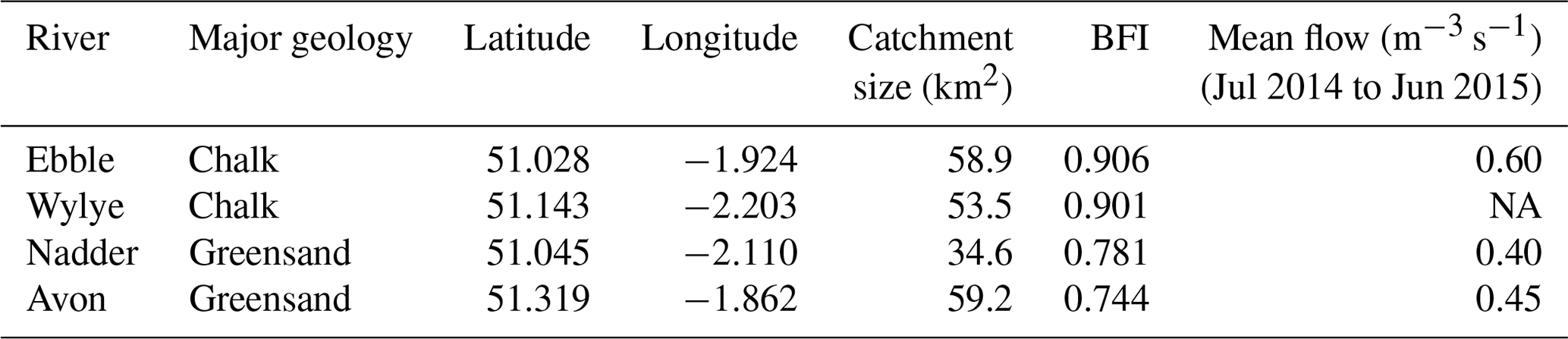
BFI: base flow index. Sources: Heppell et al. (2017) and for flow data, Heppell and Binley (2016). NA: not available.
2.2 Instrumentation and data analysis
Dissolved oxygen and temperature were logged continuously using miniDOT data loggers (Precision Measurement Engineering, Inc.) at a resolution of 0.01 mg L−1 and logging frequency of 1 min from mid-August 2014 to mid-August 2015. The DO time series for the miniDOTs was smoothed using a 30 min time step with the change in DO (ΔDO) at each minute computed from the smoothed time series. From this, the time at which ΔDO=0 was identified and the associated value of the DO deficit was noted. Dissolved oxygen at saturation was calculated using tables provided by United States Geological Survey (USGS, 2015) in accordance with Standard Methods of the American Public Health Association (1998), using both water temperature and atmospheric pressure, with atmospheric pressure data provided by British Atmospheric Data Centre. For the nighttime regression calculation, those data points that incorporated daytime values as a consequence of the implemented moving average were excluded from the regression. The data reported in this study is available from the NERC data centre (Heppell and Parker, 2018).
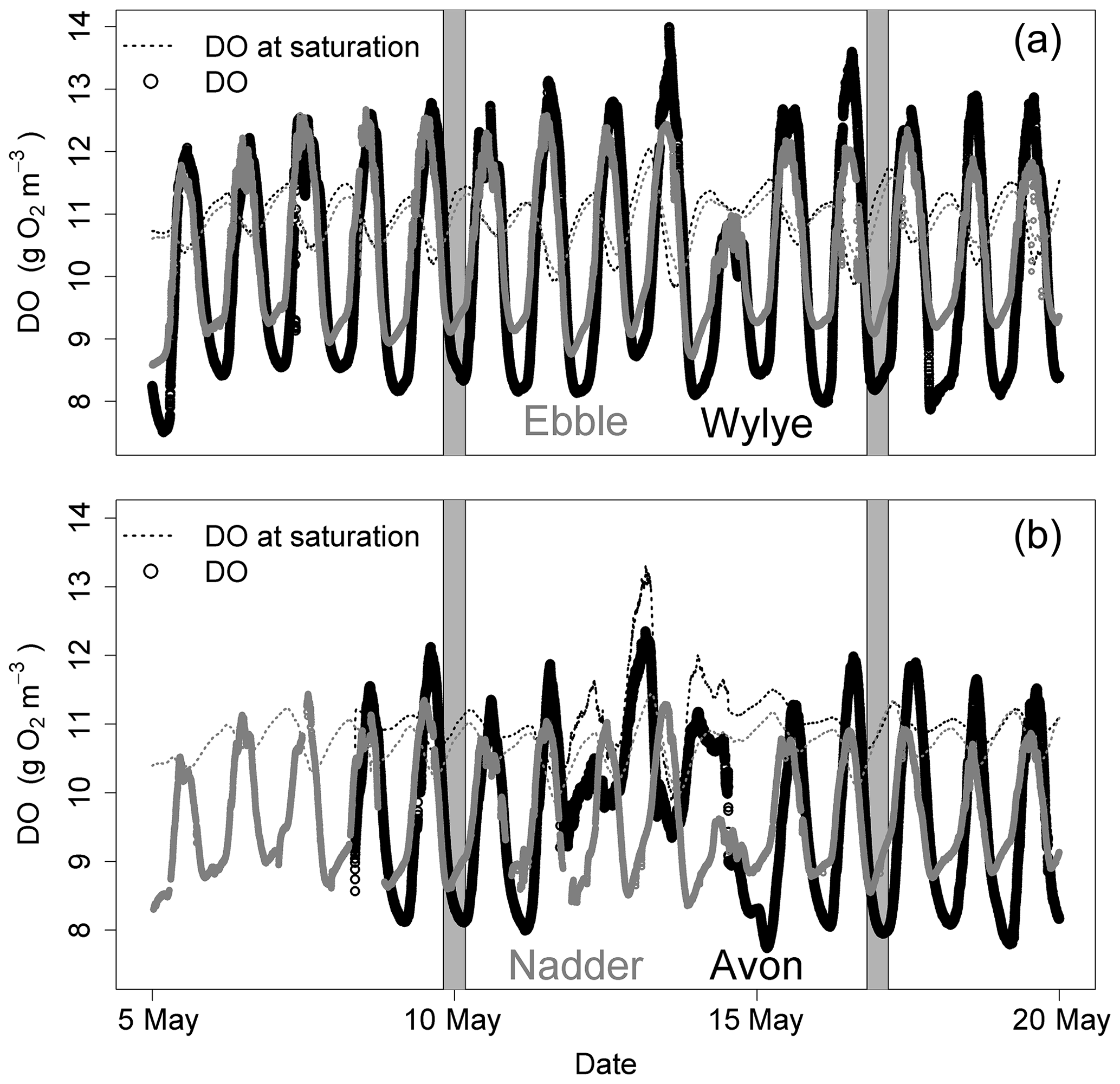
Figure 1DO time series for 5 to 20 May 2015 for two Chalk streams (a) and two Greensand streams (b). Solid grey areas are the nights of 9/10 and 16/17 May.
Figure 1 shows the DO time series (raw data) for a 2-week period in May 2015. For the two Chalk rivers, daytime DO consistently rises above DOsat typically by 1 to 3 mg DO per litre for the Wylye and 1 to 2 mg DO per litre for the Ebble. For the Greensand rivers, the Nadder rarely rises above saturation, and although the Avon does so, nevertheless not as regularly as the two Chalk rivers. The Avon shows anomalous behaviour for 13 and 14 May. Average daily DO maxima are 12.7, 12.2, 11.7 and 10.9 mg DO per litre for the Wylye, Ebble, Avon and Nadder respectively, so that prima facie the Wylye is the most productive. Peak daytime DO for the Wylye tends to happen later than that for the Ebble, as does the peak for the Avon compared to the Nadder, so that for example in the daytime of 16 May, DO for the Ebble and Wylye rises to 12 mg DO per litre, after which DO in the Ebble declines whilst DO in the Wylye continues to rise to 13.5 mg DO per litre. Note also that for the Ebble nighttime DO reaches a minimum early each night, after which it rises throughout the night, whereas the Wylye shows two types of behaviour, so that for example on the nights of 13/14 and 16/17 May, minimum DO occurs early whereas for 6/7 and 9/10 minimum DO occurs much later in the night. This behaviour is summarised in Fig. 2, with DO distributions shown in Fig. 2a and DO expressed as percent saturation averaged by time after sunrise shown in Fig. 2b. DO saturation levels for the Ebble and Nadder typically plateau at just after solar noon, whereas those for the Wylye and Avon continue to rise until 2 to 4 h after solar noon. For nighttime, DO saturation levels for the Ebble and Nadder reach a minimum relatively rapidly after sunset after which they increase slightly, particularly the Nadder, whereas for the Avon they decline throughout the night.
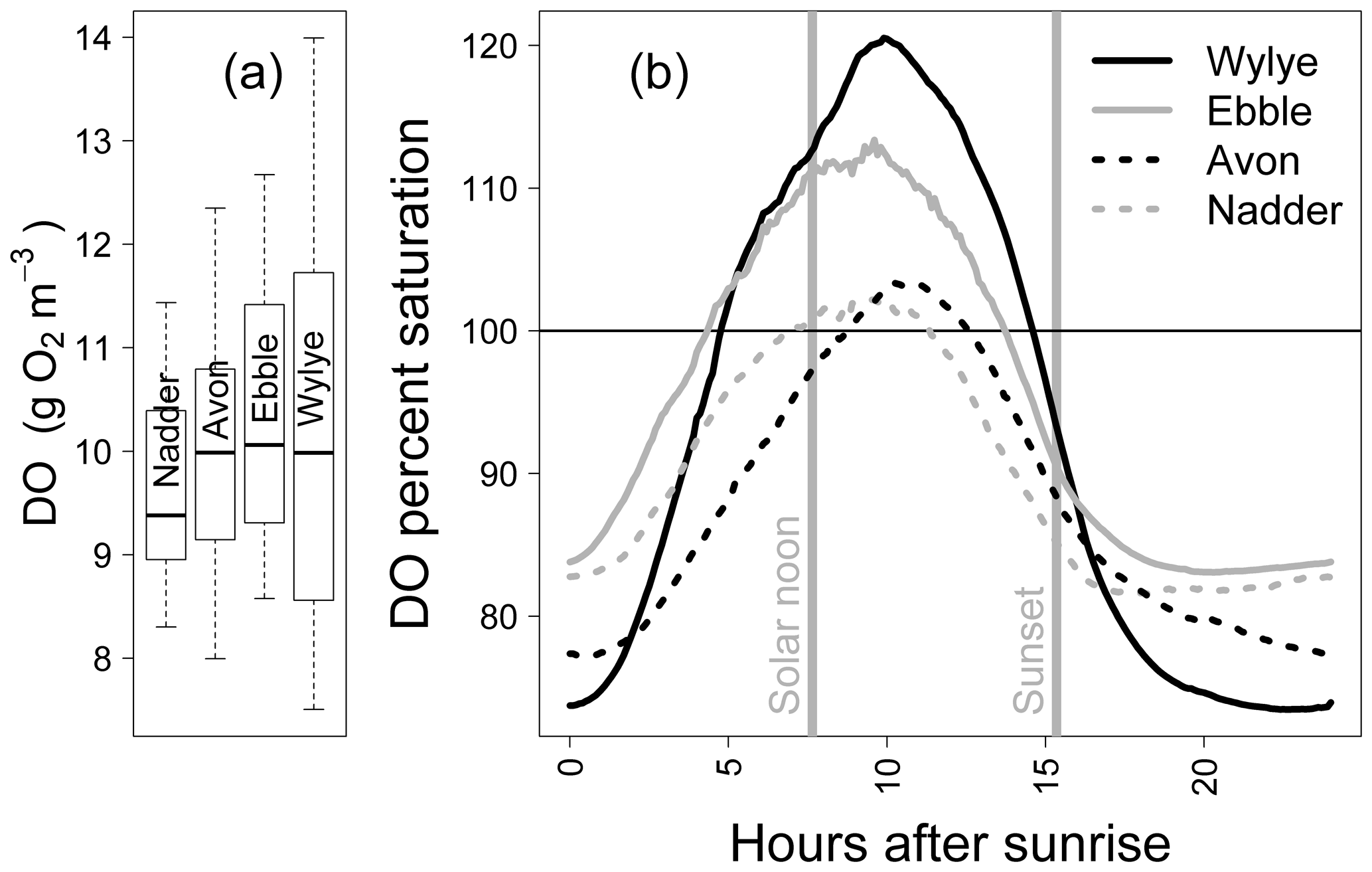
Figure 2Distributions of DO values (a) and mean DO percent saturation by hours after sunrise (b) for 5 to 20 May 2015.

Figure 3Analysis of lagged differences in DO between normalised DO time series. (a) Ebble and Wylye, (b) Ebble and Nadder (c) cross-correlations for four rivers for 5 to 20 May 2015.
In fact, the behaviour of the Ebble in terms of timing (i.e. phase) is much closer to that of the Nadder than to the behaviour of the Wylye. Figure 3 (panels a and b) shows the distributions of differences in DO at different lag intervals between normalised (that is, mean DO is first subtracted) DO time series for the Wylye, Ebble and Nadder. Each box plot is the distribution of the difference in DO for two of those time series, with one time series having been time-shifted by the number of minutes shown on the x axis. Of the two Chalk streams (Ebble and Wylye, panel a), the Wylye tends to respond later than the Ebble and is phase-shifted by approximately 90 min, whereas for the Ebble and Nadder (panel b), both systems respond at approximately the same time. The cross-correlations in Fig. 3c summarise the relative timings for all four rivers; the correlation is stronger for the Ebble and Wylye and for the Ebble and Nadder than it is for the Wylye compared to the Avon and also the Nadder compared to the Avon (for which anomalous data of 13 and 14 May was removed prior to analysis). Nevertheless, for the whole time series, the Avon lags the Nadder by approximately 2 h, which is consistent with Fig. 2. Thus, in terms of typical DO magnitudes, the two Chalk streams are similar (Fig. 2a), but in terms of phase the Ebble is similar to the Nadder.
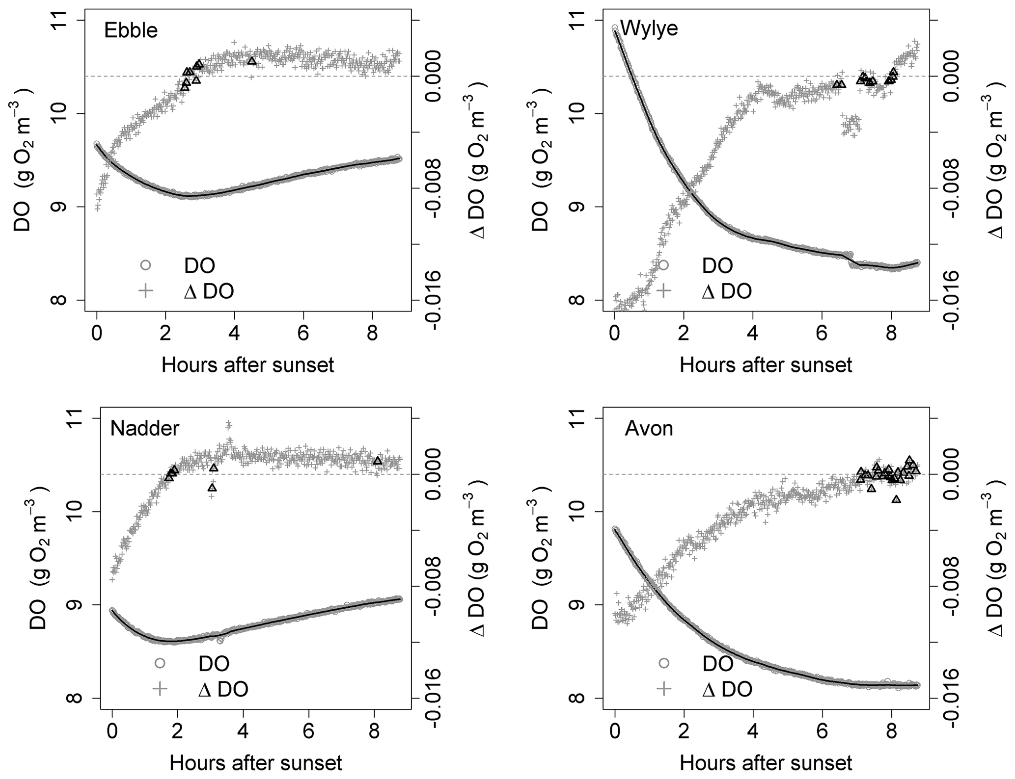
Figure 4Time series for DO and ΔDO for the night of 9 to 10 May. ΔDO is at 1 min intervals. Bold triangles mark those points where there was a change in sign of ΔDO.
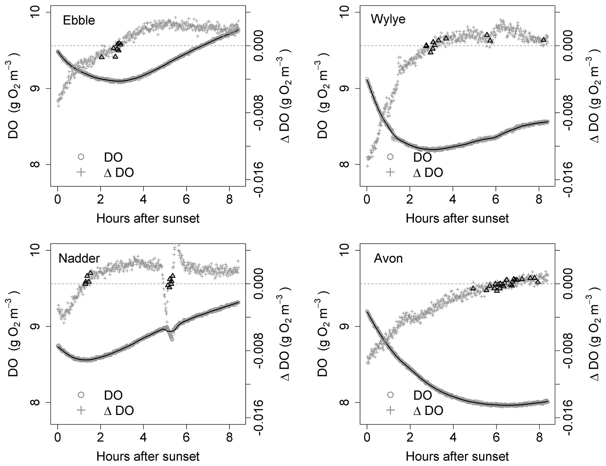
Figure 5Time series for DO and ΔDO for the night of 16 to 17 May. ΔDO is at 1 min intervals. Bold triangles mark those points where there was a change in sign of ΔDO.
For the time series shown in Fig. 1, the nights of 9 to 10 May and of 16 to 17 May are shown as examples in Figs. 4 and 5 showing both raw DO data (grey circles) and a 30-point DO moving average (solid black line), together with associated changes in DO at each minute. The changes in DO are computed using the 30-point DO moving average, not the raw data. Black triangles are those points where ΔDO=0, discussed further below. At sunset, the Wylye shows the greatest rate of DO decline of −0.016 g O2 m−3 min−1. The Ebble and the Nadder each experience approximately half that rate, with the Nadder considerably less on 9/10 May. For the Avon, the initial rate of decline is intermediate between those at about −0.010 g O2 m−3 min−1. For all four rivers, the rate of decline at sunset is higher on 9 than on 16 May. For the Ebble, there is a saddle at approximately 1 h after sunset where there is a sudden drop in the rate of decline. The main feature of the ΔDO plots, however, is the difference in timing of the point at which ΔDO=0, where for the Ebble and the Nadder it occurs between 1 and 3 h after sunset, for the Avon between 6 and 8 h after sunset but for the Wylye on 9 May it occurs late at 7.5 h after sunset and on 16 May it occurs early at 3 h after sunset.
Identification of the point at which there is zero change in DO is not as straightforward as at first it seems; the change in DO for any 1 min time step may be very close to, but never equal to, zero because of short-term stochastic variability in the DO signal. Identification could be achieved by fitting a line to the points in Fig. 4 and noting where the line crosses ΔDO=0, but this presupposes a particular model structure which may be invalid. There are two other approaches, both of which have limitations and both of which were implemented as a mutual check. One method (Method 1) is to locate the point during the night at which DO is at a minimum. One limitation is that there may be multiple local minima because of short-term DO fluctuations, any of which could be the “true” global minimum for that night. The main limitation, however, is that DO may decrease throughout the night such that minimum DO occurs at the end of the night and ΔDO itself is never equal to zero. Therefore, as a safeguard, in the implementation of Method 1, if the minimum DO was found to occur within 20 min of sunrise, that outcome was discarded. The third approach (Method 2) is to compare each pair of contiguous data points in the smoothed DO time series and to identify those points where ΔDO changes sign (from negative to positive). These are shown as black triangles in Figs. 4 and 5, which gives a range of DODzero ΔDO values. For example, for the Wylye for 16/17 May there are 11 data points where ΔDO changes sign from negative to positive, with associated values of the DO deficit ranging between 3 and 3.18 mg DO per litre with a median value of 3.06 occurring at 3 h and 9 min after sunset. For the Ebble, corresponding numbers are 1.57 to 1.73 with a median of 1.7 mg DO per litre occurring at 2 h and 46 min after sunset. The median value of those points can then be taken as the single value of the DO deficit where ΔDO=0. The drawback of this approach is that there may be anomalous data points (for example the Nadder in Fig. 5), which might yield erroneous DODzero ΔDO values.
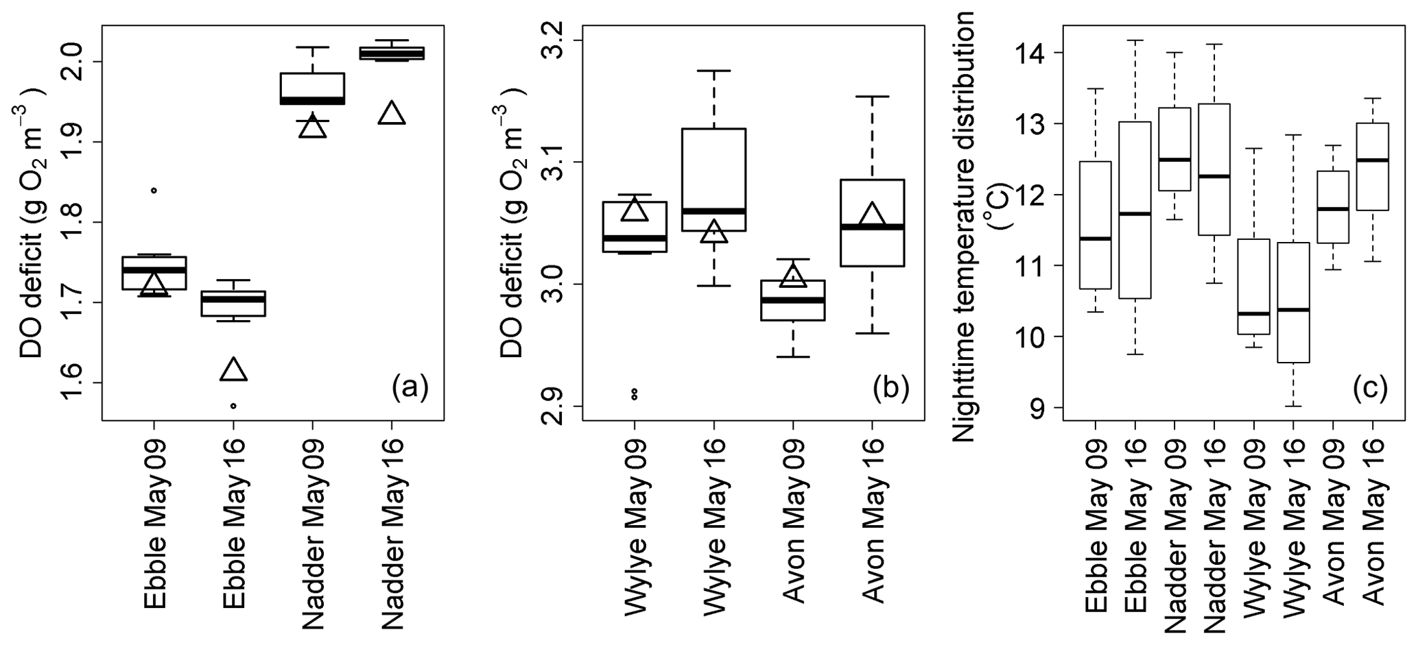
Figure 6Box plot time series of DO deficits at points of steady-state DO for the nights of 9/10 and 16/17 May 2015 for Ebble and Nadder (a) and Wylye and Avon (b). Values for the regression quotient are shown as triangles. Panel (c) shows corresponding distributions of nighttime temperatures.
For the same two nights, the sets of DODzero ΔDO values are shown as box plots (Fig. 6). Also shown (black triangles) are the corresponding values of the regression quotient calculated from the nighttime regression method. For the Ebble and the Nadder (panel a), the regression quotient underestimates the range of DODzero ΔDO values. For the Avon (panel b), the regression quotient slightly overestimates the median DODzero ΔDO value for 9/10, but on 16/17 the values are equal to one another.
For the Wylye (panel b), the regression quotient overestimates on 9/10 and underestimates on 16/17. Thus, on the night when the DO minimum comes early after sunset and the Wylye behaves more like the Ebble and the Nadder in terms of timings of DO dynamics, the regression quotient underestimates the median DODzero ΔDO value. Assuming constant R and constant k, corresponding optimised simulations for 16/17 (using “deSolve” and “FME” R libraries, Soetaert et al., 2010; Soetaert and Petzoldt, 2010) for the Ebble and Avon are shown in Fig. 7. The fit for both Ebble and Avon appears to be good, but the residuals for the Ebble are highly non-stationary. It is possible that these patterns arise because of a failure to incorporate effects of temperature on reaction kinetics of R and k. However, distributions of nighttime temperatures (Fig. 6c) do not suggest that the Ebble and Nadder have one temperature regime and the Wylye and Avon have another. In fact, the temperature regimes for the Nadder and Avon are more similar to one another than those for the Nadder and Ebble, even though the Nadder and Ebble are the rivers with early DO nighttime minima, so temperature does not appear to explain the differences in behaviour.
For data covering the entire study period (August 2014 to August 2015), the distribution of the ratio of median DODzero ΔDO values to the regression quotient is shown for each river in Fig. 8. Where the ratio is greater than 1, the median DODzero ΔDO exceeds the regression quotient. For the Ebble and Nadder this is the case for about three-quarters of the nights (75 % and 73 % for Ebble and Nadder respectively) whereas the distributions are more symmetrical for the Wylye and Avon with corresponding proportions of 60 % and 44 % respectively. Note also that groundwater regimes may be similar, but oxygen regimes differ. So, for example, even though the Wylye and Ebble are both Chalk and equally groundwater-dominated with a BFI of 0.9 (Table 1), a comparison of the distributions shown in Fig. 8 suggests differing oxygen dynamics. A corresponding argument applies to the Nadder and Avon.
A time series of median DODzero ΔDO values for the entire study period is shown in Fig. 9, together with a time series of the comparison with the regression quotient. For the Ebble, median DODzero ΔDO values range between 1 and 2.5 mg DO per litre with two peaks, one in October/November 2014 and a second in summer 2015. A trough occurs in winter, before rising to values in May similar to those in the previous September. For the Wylye, values range between 2 and approximately 5 mg DO per litre; data for June 2015 onward are more volatile and consequently less clear with regard to any evident pattern. The seasonal pattern differs in that there is no November 2014 peak, with an earlier autumnal peak occurring in September 2014. Values for the Avon range between 2 and 4 mg DO per litre with peaks in October/November 2014 and a second in June/July 2015. From mid-March to mid-April and again in late May/early June, the median DODzero ΔDO for the Avon were persistently low, with values of about 1 mg DO per litre or less. These points were considered anomalous and were discarded from the analysis. For the Nadder, the median DODzero ΔDO value rises steadily from a value of 1.5 mg DO per litre at the beginning of March 2015 to approximately 2.3 mg DO per litre in late June 2015. The Nadder differs from the other three sites in that there is only one peak occurring between May and September 2015, although the caveat is that data for the first part of the time series is missing. None of the sites shows a marked difference in behaviour according to whether Method 1 or Method 2 is used.
Also shown (Fig. 9) is a comparison between median DODzero ΔDO value () and the regression quotient (), expressed as the ratio of the former to the latter. For the Wylye and the Avon, this ratio is very close to 1 over most of the year. For the Ebble and the Nadder, however, the median DODzero ΔDO values almost always exceed the regression quotient. The notable exception is in October/November 2014 for the Ebble, where this pattern is reversed, with the regression quotient tending to exceed median DODzero ΔDO values. Whether the regression quotient overestimates or underestimates the median DODzero ΔDO value depends partly on when median DODzero ΔDO () occurs as shown for the Wylye in Fig. 10; if the change in sign of ΔDO occurs relatively quickly after sunset (between 2 and 6 h after), then the regression quotient is more likely to underestimate median DODzero ΔDO and as the time after sunset increases, the regression quotient has a tendency to overestimate DODzero ΔDO values. As the time after sunset further increases, the regression quotient again underestimates median DODzero ΔDO. To demonstrate that this is not simply a seasonal effect, this pattern is shown for the entire study period (panel a) and also for the 2-month period up to 20 May 2015 (panel b).

Figure 7Nighttime simulations for 16/17 May for Ebble and Avon. For Ebble, median DODzero ΔDO is 1.7 and regression quotient is 1.6, whereas for the Avon, they are equal (3.05).
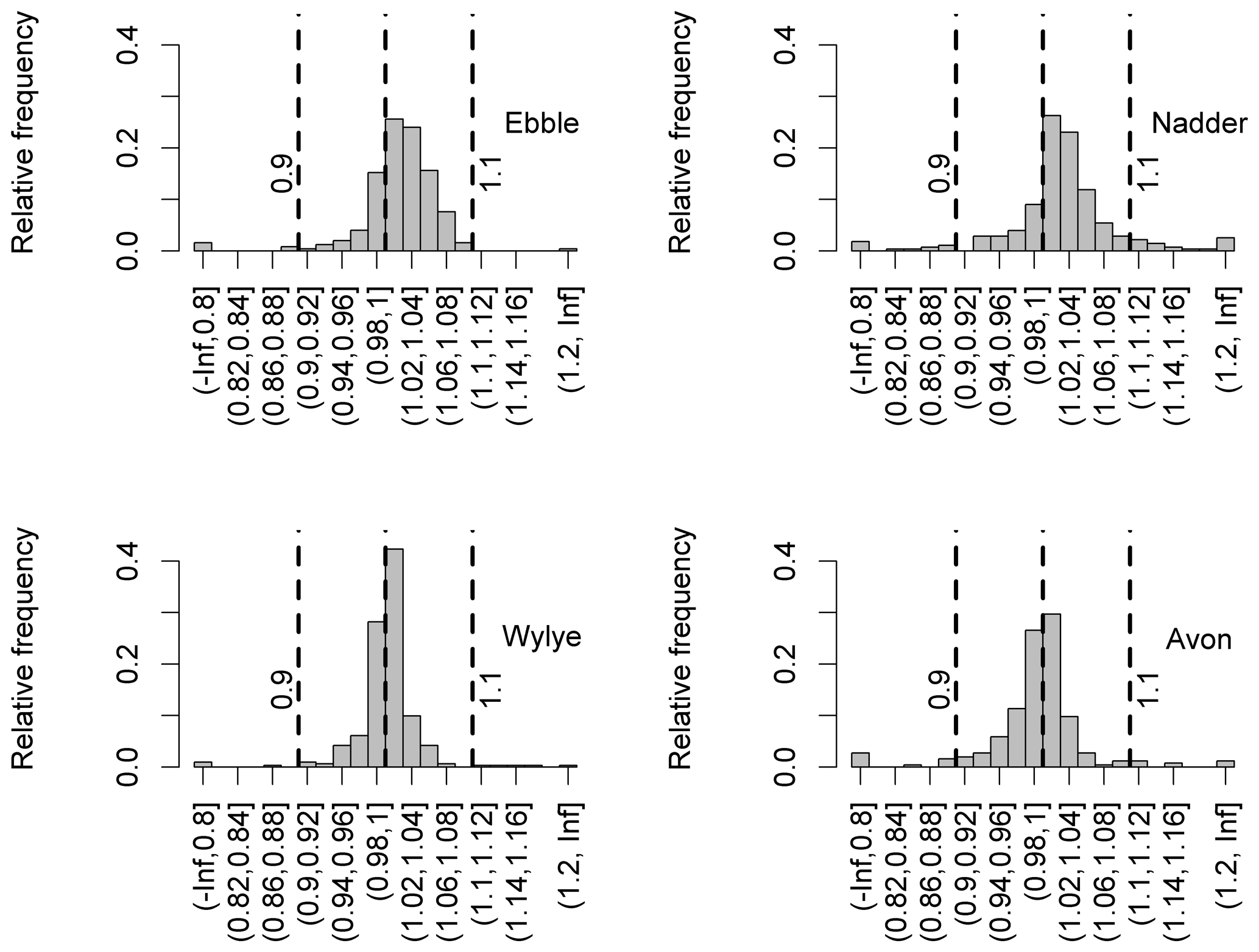
Figure 8Distributions of the ratio of DO deficit at points of zero DO change to the regression quotient.
Figure 11 shows a time series for each river relating to the length of time after sunset at which median DODzero ΔDO occurs. For September 2014 to February 2015, this interval is notably variable for all rivers, ranging between 2 and 10 h. For May to July 2015, the Ebble and Nadder show a clear pattern of a reduction in time to DODzero ΔDO. For the Nadder, this remains relatively constant at between 2 and 3 h. For the Ebble, DO reaches its minimum point most quickly in May at approximately 3 h after sunset, but then rises steadily through approximately 4 h in June, 5 h in July and 6 h after sunset in August. For the Wylye, DODzero ΔDO in May and June 2015 occurs typically at just under 5 h after sunset. Despite the fact that at other times of the year, the time interval is more variable, nevertheless the annual pattern as indicated by the trend line shows a clear periodicity with a maximum of approximately 10 h in winter (November to January) for all rivers with river-specific patterns in spring and summer.
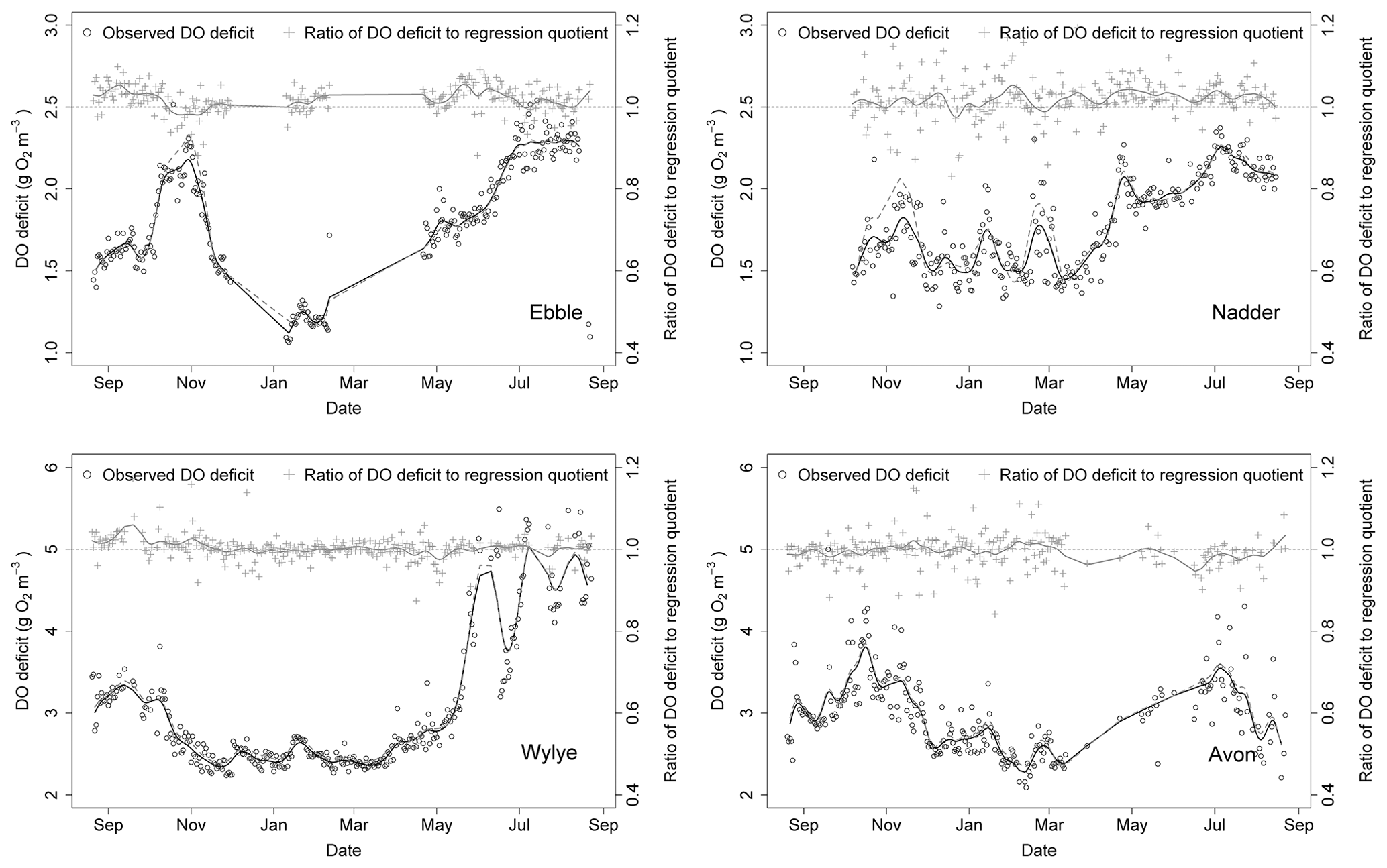
Figure 9Time series (2014–2015) of the DO deficit at points of zero DO change (black circles) and comparison with corresponding ratio derived from nighttime regression (grey crosses). Trend lines are shown for both time series. For grey dashed line (Nadder), see text.
The regression quotient up to this point was computed using all data points for any given night. An alternative would be to calculate the regression quotient using only a subset of nighttime points. One possibility would be to do so using only those data points clustered around the time after sunset at which ΔDO=0. The effect of this is shown for the Nadder in Fig. 12, which compares the regression quotient for each night in the year, calculated using all data points for each night, with that obtained using only those data points that are recorded within 15 min before or after the time where ΔDO=0. By restricting the nighttime regression calculation to those points, the bias is seen to be removed. This does not necessarily mean that the associated estimates of R and k are better, but it might mean that comparisons between nights are more consistent, although this possibility was not investigated further.
For four sites on four separate rivers, two Chalk (Wylye and Ebble) and two Greensand (Avon and Nadder), DO data were analysed for the period August 2014 to August 2015 with particular focus on a 2-week period in May 2015. For each night in the year, the nighttime dissolved oxygen deficit at points of zero DO change (DODzero ΔDO) was identified and used as a proxy for the ratio of community respiration to the volumetric aeration rate constant. This ratio was compared to a theoretical equivalent, the regression quotient, computed using the nighttime regression method (Hornberger and Kelly, 1975). The objective in comparing these ratios was to provide an aid in assessing the validity of assuming single-stage respiration. When daily median DODzero ΔDO values were compared to daily regression quotient values for the year as a whole, the regression quotients for the Ebble and Nadder persistently underestimated median DODzero ΔDO values. Additionally, for the May period, although the two Chalk rivers were more alike in terms of DO magnitudes, timings for the Ebble (times of daily DO maxima and minima) were very close to those of the Nadder, with DODzero ΔDO occurring relatively quickly after sunset. For the year, using the Wylye as an exemplar, it was shown that the regression quotient typically underestimates DODzero ΔDO when DODzero ΔDO occurs relatively quickly after sunset.
Typically, single-station DO models assume constant R and k (notwithstanding temperature effects) over the course of a single night. The analysis set out above provides a method of assessing the extent to which the assumptions of the single-stage R oxygen dynamics model are satisfied. Assume both R and k are constant and given (at nighttime) that the following relationship holds:
then
-
A plot of ΔDO against (DOsat−DO) will give a straight line with slope k and constant term R. This is used to calculate a ratio R∕k (ratio 1). and
-
At the point where ΔDO is zero, the oxygen saturation deficit (DOsat−DO) is measured. This gives a different method of calculating the same quantity, R∕k (ratio 2).
If Eq. (1) adequately describes the nighttime DO dynamics, then ratio 1 will be equal to ratio 2. If, however, they diverge significantly, then the assumptions are not satisfied. For 16 May, for example, for the Ebble, ratio 1 is 1.6 and ratio 2 is 1.7, but for the Avon, they are equal (3.05), and the corresponding simulations (Fig. 7) show clear differences in the pattern of residuals.
In itself, this divergence does not demonstrate that R is not constant, but that model assumptions are not upheld. One other possibility is that k is variable. Of course, k may differ across sites, but in order to violate model assumptions it must change both within the course of a single night and according to the same pattern for several nights in a row (as for the Ebble in May 2015). Changes in discharge and wind speed could be expected to have an impact on k. However, there is no difference in the discharge (data not shown) that would account for differences between Ebble and Avon. It could be that wind speed is changing every night in a consistent manner and therefore k is changing, but changes in the wind speed would be similar across all sites. Therefore, changes in wind speed could only account for the behaviour if the Wylye and Avon were sheltered, and buffered from the effects of changes in wind speed. However, wind speeds tend to drop during the night, so that, if for the Ebble and Nadder, a variable k were explained by falling wind speed, then one would expect DO to stagnate as the night progresses, but the reverse is the case.
On the other hand, ecosystem respiration is known to change over a single diurnal cycle (Staehr et al., 2010; Sadro et al., 2014; Alnoee et al., 2014). Schindler et al. (2017) suggest that increases in nighttime oxygen concentrations, as is the case for both the Ebble and the Nadder in May (Figs. 4 and 5), might be indicative of two-stage ecosystem metabolism. Increasing nighttime DO could be brought about by falling water temperature alone, but nighttime water temperature declines for all four sites, yet only the Ebble and Nadder consistently register increases in nighttime DO percent saturation (Fig. 2). The fact that the Ebble and Wylye exhibit similar DO ranges in May, yet the daytime Ebble DO peak typically occurs earlier could indicate that for the Ebble, as photosynthesis progresses, some products of that process are aerobically consumed. There is, however, an important caveat. Of the four rivers, the Wylye records the highest DO concentrations so that there is a prima facie case that the Wylye is the most productive. Although there were nights during which the Wylye showed increases in nighttime DO, it still consistently recorded the highest daytime DO values in May 2015. Assuming that this is because the Wylye has the highest primary production, that would mean that nighttime rises in DO maybe sufficient, but not necessary, as indicators of productive aquatic systems.
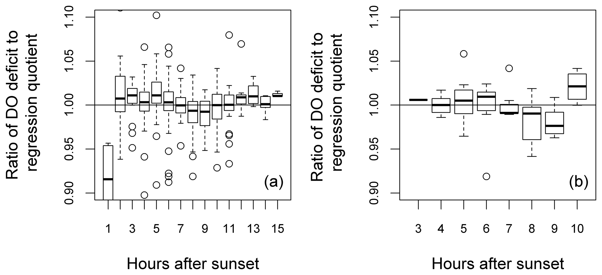
Figure 10Relationship between time after sunset until the point of zero DO change and the ratio DODzero ΔDO: (regression quotient) for the river Wylye for the entire study period (a) and the 2-month period up to 20 May 2015 (b). Hours after sunset are rounded to the nearest whole hour.

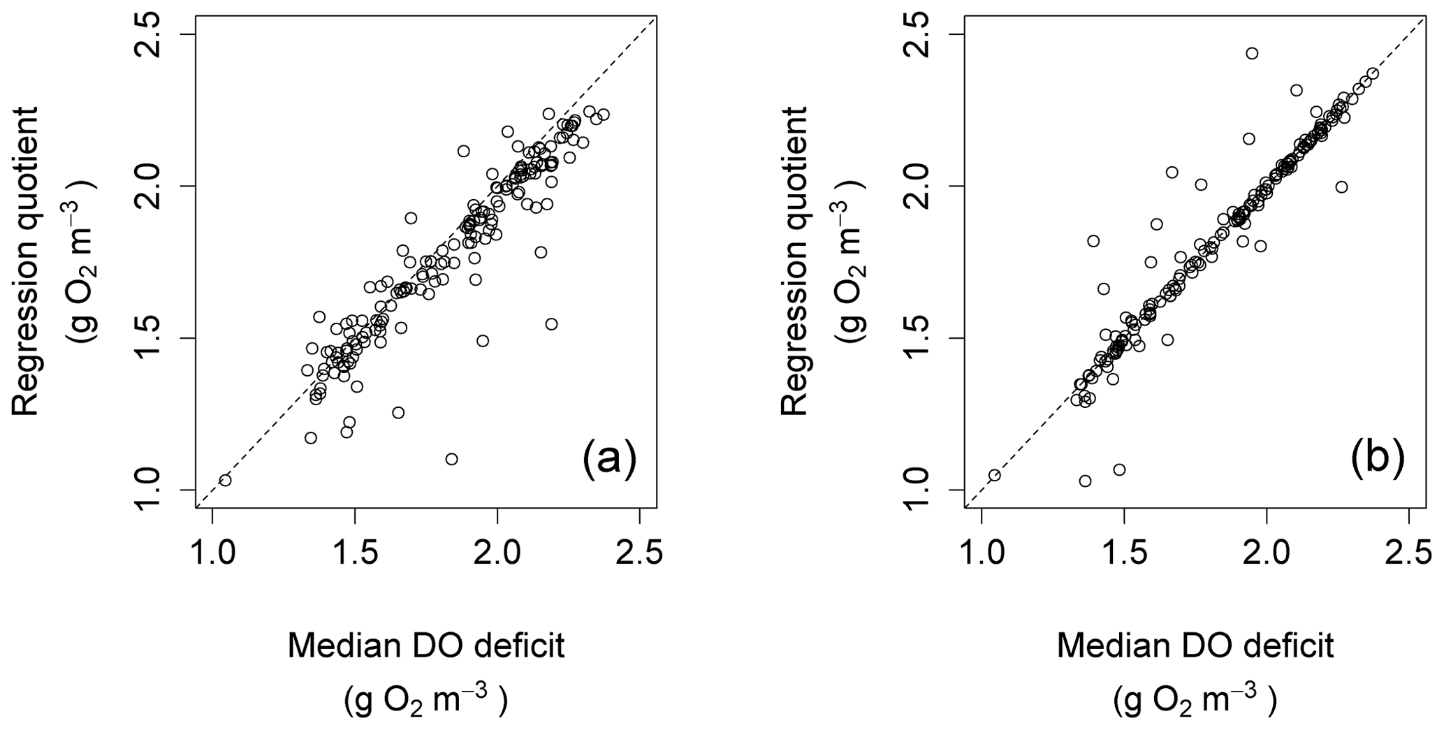
Figure 12Scatter plots for regression quotient against median DO deficit at points of zero DO change for the Nadder.
No part of the analysis presented above demonstrates, however, that R varies over the course of a day, just that the single-stage R model structure is less appropriate in some cases and that this is more likely to be explained by a variable R than by a variable k. There may be other confounding factors in the analysis, such as probe drift, but simulations (supplementary analysis) incorporating an assumed probe drift did not alter the conclusions. If the divergence is explained by other factors, this still means that those other factors, whatever they may be, are not incorporated into the model. The use of the single-stage R model to characterise or quantify aspects of stream metabolism and DO dynamics is more appropriate for some streams than others, so it is important to identify the correct model for each river system and indiscriminate application of the single-stage R diel oxygen model can result in misleading inferences when comparing different sites.
Behaviour of DO dynamics were also examined with regard to hours after sunset at which ΔDO is zero. Typically, a DO time series will be presented with time marked as civil time in a particular time zone, but framing time in terms of the behaviour of the sun both makes inter-site comparisons more transparent and also is more pertinent to the response of the aquatic plant community. It also means that, by identifying as an annual time series, the time after sunset at which ΔDO is zero, anomalous behaviour can also be identified and used either as a filter to remove spurious data or as a flag to search for particular events, for example floods or periods of unusually low flow.
The regression quotient was calculated for the night as a whole and also by restricting the data points included to those ±15 min either side of the point at which change DO is zero. This was found to remove the bias. This does not mean that calculations of R and k using only those points will give better estimates of R and k, since if there is two-stage metabolism, then such an approach would be disregarding the photosynthetic-dependent R, although it might mean that intra-stream comparisons over a series of nights are more consistent.
This paper began with a comment on the proliferation of automatic logging devices which vastly increases the potential for analysis of river oxygen and therefore river carbon dynamics. Oxygen dynamics are often analysed using models that make simplifying assumptions about the underlying processes, specifically about the constant values of both community aerobic respiration and the reaeration rate constant over the course of a single day. However, there is a debate about the extent to which respiration in particular can be represented by a single daily value. Through analysis of the dissolved oxygen deficit at points of zero DO change for four sites on four rivers, it was shown here that the assumption of constant values for either respiration or the aeration rate constant was violated perennially for two of those sites. It was suggested that this is likely to be because of two-stage rather than one-stage respiration, although it should be noted that variability in the volumetric aeration rate or even unidentified factors could account for the findings. In any case, this means that the use of single station, single-stage respiration diel oxygen models might not be optimal in such cases. This is not to decry the use of such models, as the purpose of a model is to abstract from reality. However, if analysis of DO time series were to become routine with results impacting environmental policy decisions, then it would be important to understand when these models are failing rather than presume that they are fit for purpose.
Natural Environment Research Council (NERC) data at https://doi.org/10.5285/840228a7-40a1-4db4-aef0-a9fea2079987 (Heppell and Parker, 2018).
The author declares that there is no conflict of interest.
Foundation work was carried out as part of post-doctoral research at Imperial College London. Thanks to Adrian Butler for support.
This research has been supported by the Natural Environment Research Council (grant nos. NE/J01219X/1 and NE/J012106/1).
This paper was edited by Perran Cook and reviewed by two anonymous referees.
Alnoee, A. B., Riis, T., Andersen, M. R., Baattrup-Pedersen, A., and Sand-Jensen, K.: Whole-stream metabolism in nutrient-poor calcareous streams on Oland, Sweden, Aquat. Sci., 77, 207–219, 2015.
American Public Health Association (APHA): Standard Methods for the Examination of Water and Waste Water, 20th Edn., American Public Health Association, Washington, DC, 1796 pp., 1998.
Appling, A. P., Hall, R. O., Yackulic, C. B., and Arroita, M.: Overcoming equifinality: Leveraging long time series for stream metabolism estimation, J Geophys. Res.-Biogeo., 123, 624–645, 2018.
Beaulieu, J. J., Arango, C. P., Balz, D. A., and Shuster, W. D.: Continuous monitoring reveals multiple controls on ecosystem metabolism in a suburban stream, Freshwater Biol., 58, 918–937, 2013.
Benjamin, J. R., Bellmore, J. R., and Watson, G. A.: Response of ecosystem metabolism to low densities of spawning Chinook Salmon, Freshw. Sci., 35, 810–825, 2016.
Cole, J. J., Prairie, Y. T., Caraco, N. F., McDowell, W. H., Tranvik, L. J., Striegl, R. G., Duarte, C. M., Kortelainen, P., Downing, J. A., Middelburg, J. J., and Melack, J.: Plumbing the global carbon cycle: integrating inland waters into the terrestrial carbon budget, Ecosystems, 10, 172–185, 2007.
Correa-Gonzalez, J. C., Chavez-Parga, M. D. C., Cortes, J. A., and Perez-Munguia, R. M.: Photosynthesis, respiration and reaeration in a stream with complex dissolved oxygen pattern and temperature dependence, Ecol Model, 273, 220–227, 2014.
Demars, B. O., Thompson, J., and Manson, J. R.: Stream metabolism and the open diel oxygen method: Principles, practice, and perspectives, Limnol. Oceanogr.-Meth., 13, 356–374, 2015.
Duarte, C. M., Marbà, N., Gacia, E., Fourqurean, J. W., Beggins, J., Barrón, C., and Apostolaki, E. T.: Seagrass community metabolism: Assessing the carbon sink capacity of seagrass meadows, Global Biogeochem. Cy., 24, 1–8, 2010.
Glud, R. N.: Oxygen dynamics of marine sediments, Mar. Biol. Res., 4, 243–289, 2008.
Grace, M. R., Giling, D. P., Hladyz, S., Caron, V., Thompson, R. M., and MacNally, R.: Fast processing of diel oxygen curves: Estimating stream metabolism with BASE (BAyesian Single-station Estimation), Limnol. Oceanogr.-Meth., 13, 103–114, 2015.
Heppell, C. M. and Binley, A.: Hampshire Avon: Daily discharge, stage and water chemistry data from four tributaries (Sem, Nadder, West Avon, Ebble), NERC Environmental Information Data Centre, https://doi.org/10.5285/0dd10858-7b96-41f1-8db5-e7b4c4168af5, 2016.
Heppell, C. M. and Parker, S. J.: Hampshire Avon: Dissolved oxygen data collected at one minute intervals from five river reaches, NERC Environmental Information Data Centre, https://doi.org/10.5285/840228a7-40a1-4db4-aef0-a9fea2079987, 2018.
Heppell, C. M., Binley, A., Trimmer, M., Darch, T., Jones, A., Malone, E., Collins, A., Johnes, P., Freer, J., and Lloyd, C.: Hydrological controls on DOC : nitrate resource stoichiometry in a lowland, agricultural catchment, southern UK, Hydrol. Earth Syst. Sc., 21, 4785–4802, https://doi.org/10.5194/hess-21-4785-2017, 2017.
Hornberger, G. M. and Kelly, M. G.: Atmospheric reaeration in a river using productivity analysis, J. Environ. Eng. Div., 101, 729–739, 1975.
Izagirre, O., Agirre, U., Bermejo, M., Pozo, J., and Elosegi, A.: Environmental controls of whole-stream metabolism identified from continuous monitoring of Basque streams, J. N. Am. Benthol. Soc., 27, 252–268, 2008.
NFRA (National River Flow Archive): Gauging station 43021 – Avon at Knapp Mill, available at: https://nrfa.ceh.ac.uk/data/station/info/43021, last access: on 13 October 2018.
Odum, H. T.: Primary Production in Flowing Waters1, Limnol. Oceanogr., 1, 102–117, 1956.
Pennington, R., Argerich, A., and Haggerty, R.: Measurement of gas-exchange rate in streams by the oxygen-carbon method, Freshw. Sci., 37, 222–237, 2018.
Reimers, C. E., Özkan-Haller, H., Berg, P., Devol, A., McCann-Grosvenor, K., and Sanders, R. D.: Benthic oxygen consumption rates during hypoxic conditions on the Oregon continental shelf: Evaluation of the eddy correlation method, J. Geophys. Res.-Ocean., 117, 1–18, 2012.
Richmond, E. K., Rosi-Marshall, E. J., Lee, S. S., Thompson, R. M., and Grace, M. R.: Antidepressants in stream ecosystems: influence of selective serotonin reuptake inhibitors (SSRIs) on algal production and insect emergence, Freshw. Sci., 35, 845–855, 2016.
Sadro, S., Holtgrieve, G. W., Solomon, C. T., and Koch, G. R.: Widespread variability in overnight patterns of ecosystem respiration linked to gradients in dissolved organic matter, residence time, and productivity in a global set of lakes, Limnol. Oceanogr., 59, 1666–1678, 2014.
Schindler, D. E., Jankowski, K., A'mar, Z. T.. and Holtgrieve, G. W.: Two-stage metabolism inferred from diel oxygen dynamics in aquatic ecosystems, Ecosphere, 8, 1–15, 2017.
Soetaert, K. and Petzoldt, T.: Inverse Modelling, Sensitivity and Monte Carlo Analysis in R Using Package FME, J. Stat. Softw., 33, 1–28, 2010.
Soetaert, K., Petzoldt, T., and Setzer, W.: Solving Differential Equations in R: Package deSolve, J Stat. Softw., 33, 1–25, 2010.
Song, C., Dodds, W. K., Trentman, M. T., Rüegg, J., and Ballantyne IV, F.: Methods of approximation influence aquatic ecosystem metabolism estimates, Limnol. Oceanogr.-Meth., 14, 557–569, 2016.
Staehr, P. A., Bade, D., Van de Bogert, M. C., Koch, G. R., Williamson, C., Hanson, P., Cole, J. J., and Kratz, T.: Lake metabolism and the diel oxygen technique: state of the science, Limnol. Oceanogr.-Meth., 8, 628–644, 2010.
USGS (United States Geological Survey): Dissolved oxygen solubility tables, available at: http://water.usgs.gov/software/DOTABLES/, last access: 23 November 2015.
Westlake, D. F.: Comparisons of plant productivity, Biol. Rev., 38, 385–425, 1963.
Wohl, E., Hall, R. O., Lininger, K. B., Sutfin, N. A., and Walters, D. M.: Carbon dynamics of river corridors and the effects of human alterations, Ecol. Monogr., 87, 379–409, 2017.