the Creative Commons Attribution 4.0 License.
the Creative Commons Attribution 4.0 License.
 | 13 Aug 2020
Historical CO2 emissions from land use and land cover change and their uncertainty
Léa Crepin
Yann Quilcaille
Richard A. Houghton
Philippe Ciais
Michael Obersteiner
Emissions from land use and land cover change are a key component of the global carbon cycle. However, models are required to disentangle these emissions from the land carbon sink, as only the sum of both can be physically observed. Their assessment within the yearly community-wide effort known as the “Global Carbon Budget” remains a major difficulty, because it combines two lines of evidence that are inherently inconsistent: bookkeeping models and dynamic global vegetation models. Here, we propose a unifying approach that relies on a bookkeeping model, which embeds processes and parameters calibrated on dynamic global vegetation models, and the use of an empirical constraint. We estimate that the global CO2 emissions from land use and land cover change were 1.36±0.42 PgC yr−1 (1σ range) on average over the 2009–2018 period and reached a cumulative total of 206±57 PgC over the 1750–2018 period. We also estimate that land cover change induced a global loss of additional sink capacity – that is, a foregone carbon removal, not part of the emissions – of 0.68±0.57 PgC yr−1 and 32±23 PgC over the same periods, respectively. Additionally, we provide a breakdown of our results' uncertainty, including aspects such as the land use and land cover change data sets used as input and the model's biogeochemical parameters. We find that the biogeochemical uncertainty dominates our global and regional estimates with the exception of tropical regions in which the input data dominates. Our analysis further identifies key sources of uncertainty and suggests ways to strengthen the robustness of future Global Carbon Budget estimates.
- Article
(6450 KB) - Full-text XML
- BibTeX
- EndNote


The annual flux of carbon dioxide (CO2) to the atmosphere caused by land use and land cover change (LULCC) is a key part of the Global Carbon Budget (GCB; Friedlingstein et al., 2019). It is one of the two historical anthropogenic sources of CO2 (along with fossil fuel burning and industry emissions), and when added to the land carbon sink it gives the net land-to-atmosphere carbon exchange. In fact, it is so closely connected to the land carbon sink that choosing incompatible definitions for these two fluxes can lead to double counting or missing part of the budget (Gasser and Ciais, 2013). Thus, models are required to disentangle these emissions from the land carbon sink, because only the sum of both can be physically observed. The Global Carbon Budget 2019 (GCB2019) assessment (Friedlingstein et al., 2019) estimated that LULCC emissions were 1.5±0.7 PgC yr−1 (1σ range) on average over the 2009–2018 period. This value relied on two lines of evidence: dynamic global vegetation models (DGVMs), which are complex process-based and spatially explicit models of the terrestrial carbon cycle (and related processes), and bookkeeping models, which are parametric models that convolute time series of LULCC areal perturbations with empirical response functions describing changes in ecosystem carbon stocks after these perturbations.
The strengths and weaknesses of those two types of models are contrasting: DGVMs are developed to precisely describe the biogeochemistry of plants and ecosystems, albeit without overly focusing on LULCC, whereas bookkeeping models are specifically designed to evaluate LULCC emissions, although without any explicit representation of biogeochemical processes. Any comparison between those models is rendered even more difficult by two factors. First, DGVMs and bookkeeping models do not naturally follow the same definition of LULCC emissions, as DGVMs tend to include the “loss of additional sink capacity” (LASC) in their estimate (Gasser and Ciais, 2013; Pongratz et al., 2014). The LASC is defined as the difference between the actual land sink under changing land cover and the counterfactual (stronger) land sink under preindustrial land cover. The LASC, however, is not an actual physical flux: it is a foregone carbon removal. (A few DGVMs are now capable of providing LULCC emissions that are consistent with the bookkeeping definition; however, these estimates are not used to establish the best-guess estimates for the GCB (Friedlingstein et al., 2019).) The second source of discrepancy is the different historical LULCC data sets used to drive the models. In the GCB2019, the DGVMs and one of the two bookkeeping models (Hansis et al., 2015) used spatially explicit LULCC drivers from the “Land-Use Harmonization” (LUH) project (Hurtt et al., 2006, 2011). The second bookkeeping model (Houghton and Nassikas, 2017), however, used independent driving data compiled from national statistics of the United Nation's Food and Agriculture Organization (FAO), especially from its Global Forest Resources Assessment 2015 (FRA2015; FAO, 2015).
Here, using the OSCAR reduced-form Earth system model, we bridge the gap between these approaches and estimates. OSCAR embeds a bookkeeping module as well as simplified biogeochemical processes calibrated on DGVMs; this makes it a valuable tool to consistently bridge across the different estimates used in the GCB, as illustrated in Table 1. Thus, the goal of this paper is threefold: first, it is to provide another bookkeeping estimate of global and regional LULCC emissions – that will hopefully be used in the future GCB – obtained with an original model; second, it is to revise and further investigate the LASC estimates that we provided in an earlier version of the GCB (Le Quéré et al., 2018b); and, third, it is to investigate the uncertainty range in both these fluxes along the three axes of analysis shown in Table 1: the inclusion of the LASC, the driving LULCC data sets, and the biogeochemical parameterization.
Table 1Availability of LULCC emissions estimates in the GCB2019 and this study. This follows our three main axes of analysis: the definition of LULCC emissions (i), the driving data sets (ii), and the biogeochemical parameterization (iii).

a BLUE (Hansis et al., 2015) and H&N (Houghton and Nassikas, 2017) are bookkeeping models, whereas the others are DGVMs. b OSCAR could not be calibrated on these DGVMs due to insufficient data.
OSCAR is a reduced-complexity model built to emulate the behavior of more complex (typically three-dimensional and process-based) models at the yearly timescale (although it cannot generate inter-annual variability by itself). Its land carbon cycle is calibrated on DGVMs; it is not spatially resolved, but it is subdivided into 10 broad world regions and 5 biomes (see Appendix A1 for a more detailed description). The model's preindustrial steady state is calibrated on the exact same simulations made for the GCB (also called the TRENDY exercise), and it does not require any spin-up. The transient responses of net primary productivity, wildfires, and heterotrophic respiration to changes in atmospheric CO2 and climate are calibrated on Coupled Model Intercomparison Project 5 (CMIP5) simulations (Arora et al., 2013). Its bookkeeping module keeps track of ecosystems affected by LULCC separately, offering a consistent and easy way to isolate LULCC emissions from the land sink (Gasser and Ciais, 2013; Gasser et al., 2017). The LULCC activities accounted for are gross land cover change transitions, wood harvest (without land cover change), and shifting cultivation (i.e., rapid rotations between young natural ecosystems and cropland). OSCAR does not include fire as a land management tool (Houghton et al., 2012), the emissions caused by the draining and burning of peatlands (Carlson et al., 2015; Guillaume et al., 2018; Houghton and Nassikas, 2017), or the impact of LULCC on the export of terrestrial organic carbon to the ocean via the land–ocean aquatic continuum (Regnier et al., 2013). Here, we use OSCAR v3.1: an iteration over v3.0 in which the land carbon cycle's structure was slightly altered and its preindustrial steady state was recalibrated. Both changes are described in Appendix A2, and older changes that led from v2.2 to v3.0 are summed up in Appendix A3. OSCAR v2.2 has been comprehensively described by Gasser et al. (2017). These and earlier versions have been used in the past to investigate LULCC emissions (Arneth et al., 2017; Bastos et al., 2016; Eglin et al., 2010; Gasser and Ciais, 2013; Gitz and Ciais, 2003).
We follow an experimental protocol similar to that used in the recent GCBs (and fully described in Appendix A4). The model is driven with observed changes in environmental conditions (global atmospheric CO2, regional temperature, and precipitation) and with specific LULCC driving data. Thanks to the model's flexibility and low computing requirements, we also run different LULCC data sets, sensitivity experiments in which either changes in environmental conditions or LULCC are turned off, and a Monte Carlo ensemble of 10 000 different biogeochemical parameterizations. These parameterizations are drawn randomly and with equiprobability from a pool of potential sets of parameters. This main pool is obtained by combining smaller pools of available parameterizations for separate processes (or groups of processes), as described by Gasser et al. (2017). For instance, recalibration of the preindustrial steady state led to 11 possible parameterizations for preindustrial net primary productivity and turnover times, 4 for preindustrial wildfire rates, 5 for preindustrial export fractions from crop harvesting, and 2 for those from animal grazing. This is already a total of parameterizations. These are further combined with available parameterizations for other elements such as the transient response of the land carbon cycle to atmospheric CO2 and climate change or the handling of harvested wood products, which leads to a main pool of ∼1.5 million sets of parameters.
Our best-guess estimate is derived by combining the results obtained with two LULCC data sets: the latest iteration of the LUH2 data set used for the GCB2019 (Friedlingstein et al., 2019) and the FRA2015 data set used by Houghton and Nassikas (2017). However, the latter data set ends in 2015; therefore, we extended its results with constant values over the 2016–2018 period equal to the average of the 2011–2015 period. To constrain this best-guess ensemble, each of the 20 000 elements is given a weight based on how well it compares to a reference value. All results presented in this study are the ensuing weighted averages and weighted standard deviations (see Appendix A5). The chosen constraining value is the net change in the land carbon stock between 1850 and 2018, which is estimated to be PgC. It is calculated via the carbon balance over the chosen period using the GCB2019 estimates of cumulative fossil fuel emissions and changes in atmospheric and oceanic carbon stocks as well as standard uncertainty propagation.
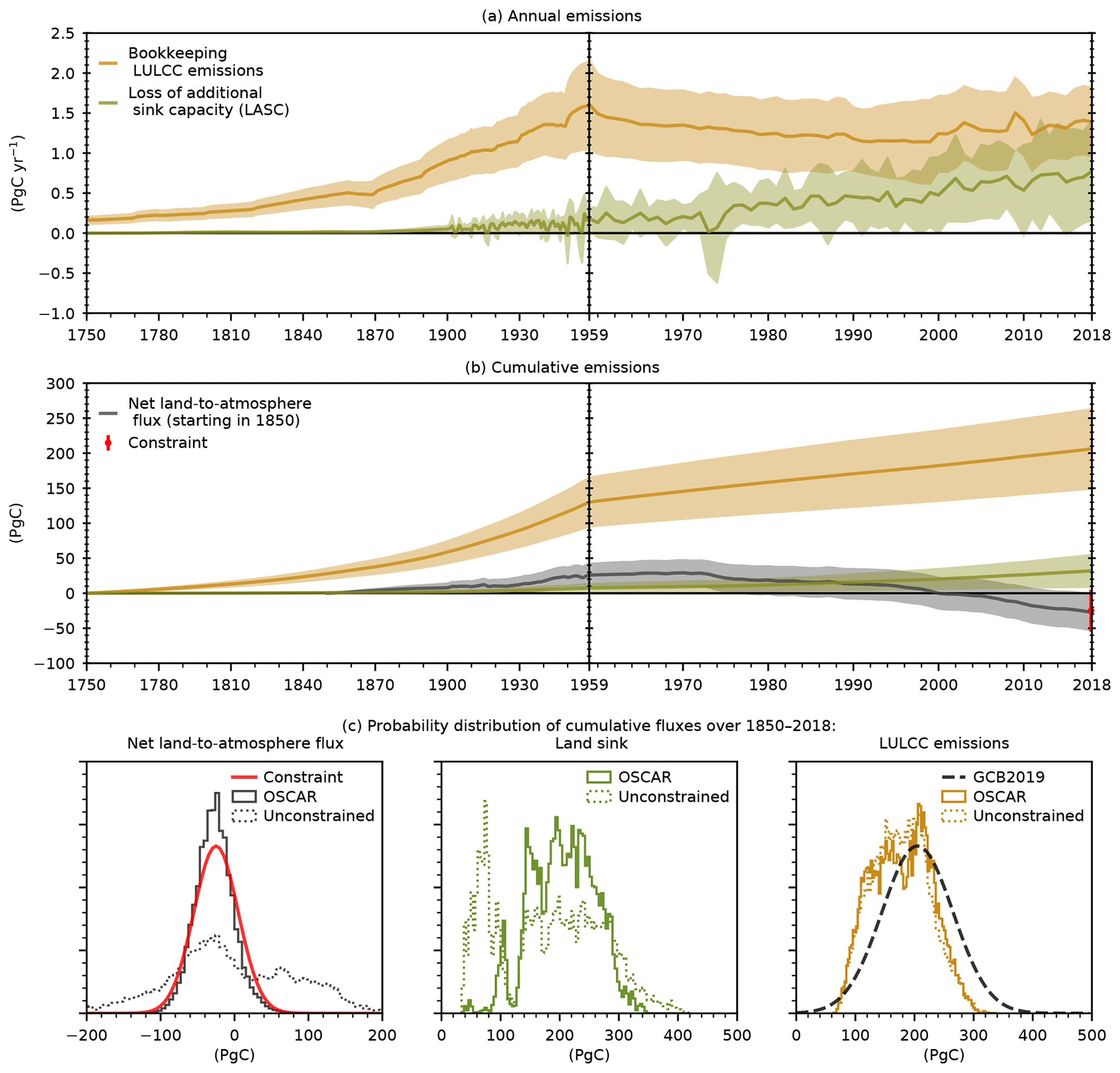
Figure 1Our best-guess estimates of bookkeeping LULCC emissions and LASC. Panel (a) shows annual fluxes, and panel (b) shows cumulative fluxes. The net land-to-atmosphere flux is also shown in panel (b) and compared with the constraint (red). Shaded areas show the 1σ uncertainty range. Panel (c) shows the detailed probability distributions of the cumulative net land flux, land sink, and LULCC emissions in the unconstrained (dotted histograms) and constrained (plain histograms) output ensemble (20 000 Monte Carlo elements) compared with the constraint (red) and the GCB estimates (dashed black).
3.1 Global LULCC emissions and LASC
Our primary results are shown in Table 2 and Fig. 1. We find global LULCC emissions of 1.36±0.42 PgC yr−1 on average over the 2009–2018 period, which is consistent with the GCB2019 estimate (Friedlingstein et al., 2019) of 1.5±0.7 PgC yr−1. Our reported value follows a bookkeeping definition (Gasser and Ciais, 2013; Pongratz et al., 2014) and is therefore comparable to that of the GCB. We simulate that historical LULCC emissions peaked at a value of 1.61±0.55 PgC yr−1 in 1959. Since then, they have remained roughly steady, but they reached a local minimum of 1.14±0.52 PgC yr−1 in 1999. Overall, we estimate that a total of 206±57 PgC was emitted between 1750 and 2018, and a total of 178±50 PgC was emitted between 1850 and 2018. These values are also consistent with the GCB2019 estimates of 235±75 and 205±60 PgC over the same periods, respectively.
Table 2Estimates of the global net land-to-atmosphere flux, LULCC emissions, land sink, and LASC. Estimates following our default (i.e., best-guess) and alternative constraints are provided. The land sink includes the LASC; therefore, the net land-to-atmosphere flux is strictly equal to the LULCC emissions minus the land sink.
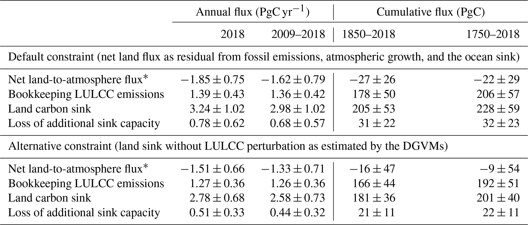
* Counted algebraically: negative values denote carbon removal from the atmosphere.
We estimate a global LASC of 0.68±0.57 PgC yr−1 on average over the 2009–2018 period. This amounted to a cumulative total of 32±23 PgC between 1750 and 2018 and to 31±22 PgC between 1850 and 2018. This extremely low difference between the two periods is explained by the nature of the LASC. It is a foregone land carbon sink – a product of both land cover change and environmental condition changes. Since environmental conditions only changed marginally during the early 1750–1850 period, the land sink and the LASC were extremely low. As the change in environmental conditions became more intense in the recent past, both fluxes increased in intensity. Our new estimates of the LASC are larger than those we reported in a past GCB (Le Quéré et al., 2018b) owing to the change in the empirical constraint. Table 2 shows that we indeed obtain estimates similar to prior estimated values by reverting back to the old constraint (which was the cumulative land sink over the 1850–2018 period without LULCC simulated by DGVMs). The performance of this alternative constraint is further discussed later in this paper and is shown in Fig. A1 in the Appendix.
The effect of the constraint is further detailed in Fig. 1c. Since the constraint is applied to the cumulative net land-to-atmosphere flux over the 1850–2018 period, it corrected the overestimate and substantially reduced the spread of this value: from an unconstrained PgC to PgC (compared with the constraining value of PgC). Applying the constraint essentially resulted in the exclusion of aberrant values of the land carbon sink without significantly affecting LULCC emissions. The cumulative LULCC emissions over the 1850–2018 period were indeed 176±48 PgC before the constraint was applied (and 178±50 PgC after). As similar processes drive the LASC and the land sink, the stronger constraining effect on the land sink is also logically visible on the LASC: the unconstrained cumulative LASC over the 1850–2018 period was 25±23 PgC (and the constrained value was 32±23 PgC).
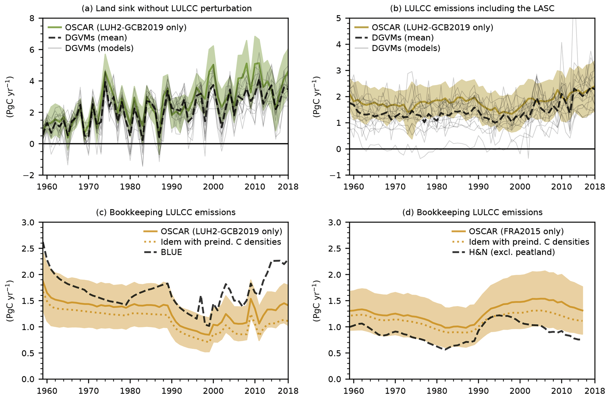
Figure 2Comparison of our results with the GCB2019. (a) The annual terrestrial carbon sink in the absence of the LULCC perturbation simulated by OSCAR (color), the individual GCB DGVMs (light gray), and their multi-model mean (dashed black). (b) The annual LULCC emissions deduced from the GCB DGVMs (i.e., including the LASC). (c) Bookkeeping LULCC emissions when the model is driven by the LUH2-GCB2019 data set compared with BLUE estimates reported by the GCB2019. The dotted line shows the same emissions but when carbon densities are kept at their preindustrial level throughout the simulation (shown without uncertainty for legibility). (d) Bookkeeping LULCC emissions when the model is driven by the FRA2015 data set compared with the H&N estimates from which emissions from peatlands were subtracted. All shaded areas show the 1σ uncertainty range. “Idem” stands for “same as above”.
3.2 Comparison with GCB models
Comparability between our best-guess estimates and those of the GCB2019 is limited (due to the differing definitions or driving data); therefore, we dedicate this section to comparing like to like. Figure 2a compares the annual land sink over the 1959–2018 period in the absence of the LULCC perturbation (i.e., with a preindustrial land cover). OSCAR simulates a slightly larger land sink by the end of the period than the DGVMs, although it remains within their uncertainty range. It also reproduces the inter-annual variability of the complex models fairly well. Note that this specific simulation is used by the GCB to define the land sink. This implies that their land sink is not comparable to ours (except in this figure), as theirs does not include the LASC. Figure 2b compares LULCC emissions calculated using the DGVMs' definition (Gasser and Ciais, 2013; Pongratz et al., 2014; i.e., including the LASC) over the 1959–2018 period. OSCAR is in line with the DGVMs, although it estimates a slightly larger flux over the beginning of the period. More importantly, it displays a much lower uncertainty range than the spread among DGVMs. Since OSCAR emulates the carbon densities of the DGVMs well (Table A1 in the Appendix), we attribute this difference in spread to the large variance in the land cover map used by the DGVMs (Table A2) and their processing of the input LULCC data set.
Figure 2c compares OSCAR and BLUE estimates of the bookkeeping LULCC emissions (i.e., without the LASC). BLUE is one of the two bookkeeping models used in the GCB2019, and both models are driven by the LUH2-GCB2019 data set. OSCAR and BLUE display similar annual variations in their LULCC emissions, but BLUE is systematically higher than OSCAR, and it is above the 1σ range of our estimates by the end of the simulation. Figure 2d compares OSCAR and H&N estimates (also without the LASC). H&N is the second bookkeeping model of the GCB2019, and this time both models are driven by the FRA2015 data set. Again, both models display similar annual variations, except near the end of the simulation, and this time H&N is systematically lower than OSCAR, although it remains mostly within its 1σ range. Given that BLUE and H&N are parameterized with the same carbon densities, one would expect that OSCAR's estimates would systematically be either higher or lower. The fact that this is not the case suggests that part of the differences between the three bookkeeping models possibly stems from other factors such as structural assumptions or ways of processing and implementing the LULCC data sets.
Table 3Uncertainty sources in our estimates of bookkeeping LULCC emissions and LASC expressed as the debiased standard deviation (1σ) and the coefficient of variation (CV; in parentheses).
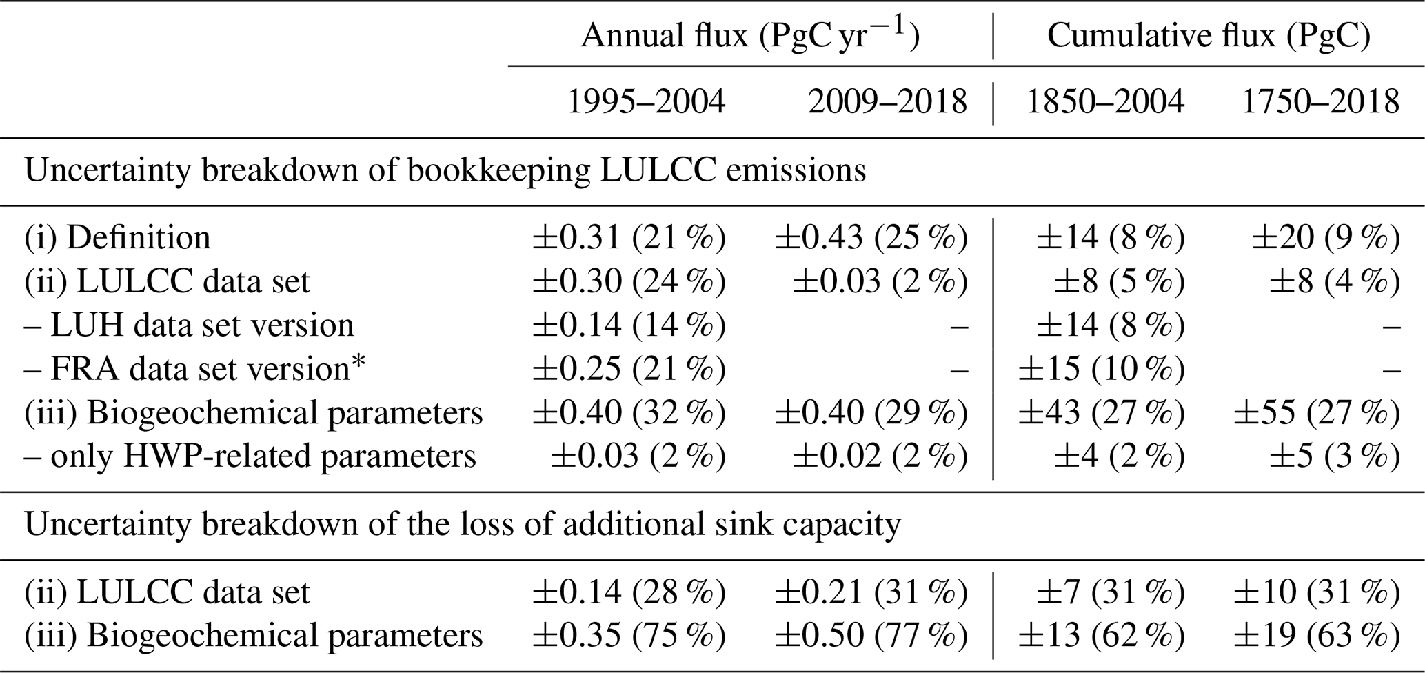
* These values were taken directly from Houghton and Nassikas (2017); therefore, they were not computed with OSCAR. They include some biogeochemical uncertainty, although to a lesser but unknown degree.
3.3 Uncertainty analysis
Although we cannot investigate the aforementioned structural differences between bookkeeping models, our experimental setup allows for the investigation of several factors within OSCAR that affect the spread in our global results. Figure 3 and Table 3 summarize this. The first factor is whether the LASC is included in the estimate of the LULCC emissions, as this is usually the case when they are calculated with DGVMs, which is illustrated in Fig. 3a. Over the last decade, the difference between including and excluding the LASC corresponds to a debiased 1σ range of ±0.43 PgC yr−1 and a coefficient of variation (CV) of ±25 % (see Appendix A6). This rather substantial value is in line with previous studies that quantified this discrepancy (Gasser and Ciais, 2013; Stocker and Joos, 2015). Because the LASC only became non-negligible in the recent past, the effect of its inclusion or exclusion on cumulative LULCC emissions is smaller than for recent annual emissions: we estimate that it is only ±20 PgC (±9 %) over the 1750–2018 period. However, it is crucial to understand that the intensity of this discrepancy will keep increasing and accumulating as long as changes in environmental conditions do not stabilize (Gasser and Ciais, 2013). This is illustrated by the positive trend in the CV in Fig. 3a. In our view, this ever-growing discrepancy strongly pleads in favor of choosing, retaining, and consistently applying one clear definition of LULCC emissions. In the following, we exclude the LASC from LULCC emissions; therefore, we discuss it separately.
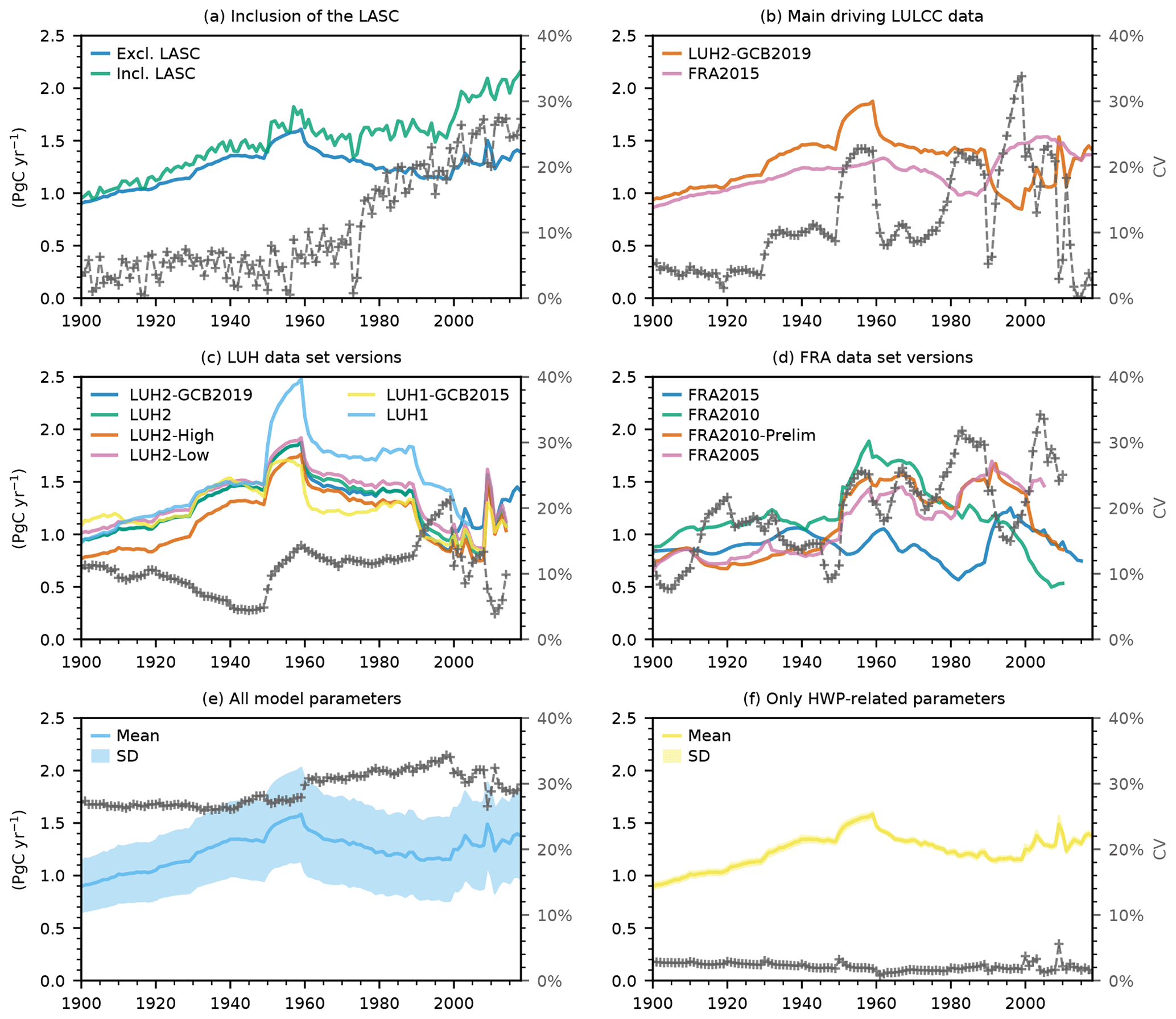
Figure 3Variations and uncertainties in the time series of global annual LULCC emissions. (a) The effect of adding the LASC to LULCC emissions. (b) The effect of the LULCC driving data sets (only the two data sets used to estimate our best guess). (c) The effect of the data set version among the LUH variants (not used for our best guess). (d) The effect of the data set version among FRA variants. These emissions were not simulated by OSCAR; they were reported by Houghton and Nassikas (2017; their Fig. 8). (e) The effect of all of the parameters of OSCAR (using the weighted Monte Carlo ensemble). (f) The effect of the subset of parameters of OSCAR that are related to harvested wood products (i.e., the parameters that are not derived from DGVMs). All panels show bookkeeping LULCC emissions with the obvious exception of panel (a). Thick colored lines show the values obtained by averaging over all axes of analysis apart from the one investigated in the panel. The dashed gray lines with markers show the debiased coefficients of variation (CVs), i.e., the ratios of the debiased standard deviation over the average, and refer to the y axis on the right-hand side of each panel.
The second factor of uncertainty is the driving LULCC data set. Figure 3b shows the difference between the average bookkeeping emission estimates based on LUH2-GCB2019 and those based on FRA2015. We find that the annual emissions from the two data sets are in particularly good agreement on average over the last decade (Table 3), although this is purely fortuitous as the discrepancy is ±0.30 PgC yr−1 (±24 %) over the 1995–2004 period and even peaks at ±0.39 PgC yr−1 (±34 %) in 1999. More worrying, perhaps, is the two data sets' disagreement on the trend in emissions after 1990. This discrepancy is hidden in our best-guess emissions that are rather even over the last 30 years. In terms of cumulative emissions over the 1750–2018 period, however, results from the two data sets are in good agreement, with only a ±8 PgC (±4 %) discrepancy. Additionally, Fig. 3c and d display the same source of uncertainty but among different versions of each of the two main data sets. This variation, which is caused by updating the data sets, is visible, for instance, when comparing older versions of the GCB with one another. We find that the difference among several versions of the same data set is of the same order of magnitude as the difference between our two main data sets. For the LUH data set, this is explained by several factors, from the simple update of the historical land cover data used as input (Klein Goldewijk et al., 2017; Klein Goldewijk et al., 2011) to the complete overhaul of how shifting cultivation is estimated (Heinimann et al., 2017). Among the FRA-based data set's versions, this difference is found to be somewhat larger. This is likely due to the concomitant update of some biogeochemical parameters of the H&N model (Houghton and Nassikas, 2017) that we cannot separate here, because the results shown in Fig. 3d are not based on OSCAR.
The third and last factor of uncertainty is the parameterization of the model (for biogeochemistry). Using our Monte Carlo ensemble, we find a weighted standard deviation of ±0.40 PgC yr−1 (±29 %) for annual emissions averaged over the 2009–2018 period and of ±55 PgC (±27 %) for emissions cumulated over the 1750–2018 period. Except in some specific years, this source of uncertainty in annual emissions is the largest of the three we studied, and it dominates without exception in cumulative emissions. Carbon densities (and the parameters determining them) are the key modeling factors explaining this spread (Gasser and Ciais, 2013). Figure 3f and Table 3 show the spread in our results when looking only at the variation caused by the parameters that relate to harvest wood products (HWPs). It is found to be one order of magnitude smaller than the total uncertainty caused by all parameters, confirming that biogeochemical parameters explain most of the uncertainty. However, we acknowledge that OSCAR likely underestimates the HWP-related uncertainty, because there is only one option to choose from (in the Monte Carlo setup) regarding how HWPs are split between pools with different decay timescales (Appendix A7).
Finally, a similar uncertainty breakdown for the LASC is reported in Table 3. We find that the uncertainty in the average annual LASC between our two main LULCC data sets over the last decade is ±0.21 PgC yr−1 (±31 %), and it is ±10 PgC (±31 %) for the cumulative LASC since the year 1750. The much higher CV in the cumulative LASC compared with that in the cumulative LULCC emissions suggests that the latter is kept relatively low thanks to compensation effects that do not come into play in the former. We also find that the biogeochemical uncertainty in the LASC is high: ±0.50 PgC yr−1 (±77 %) for the annual flux over the 2009–2018 period and ±19 PgC (±63 %) for the cumulative flux over the 1750–2018 period. These values reflect the large uncertainty in the ecosystems' response to transiently changing environmental conditions, despite our constraints (unconstrained CVs are ±98 % and ±86 % for the abovementioned time periods, respectively).
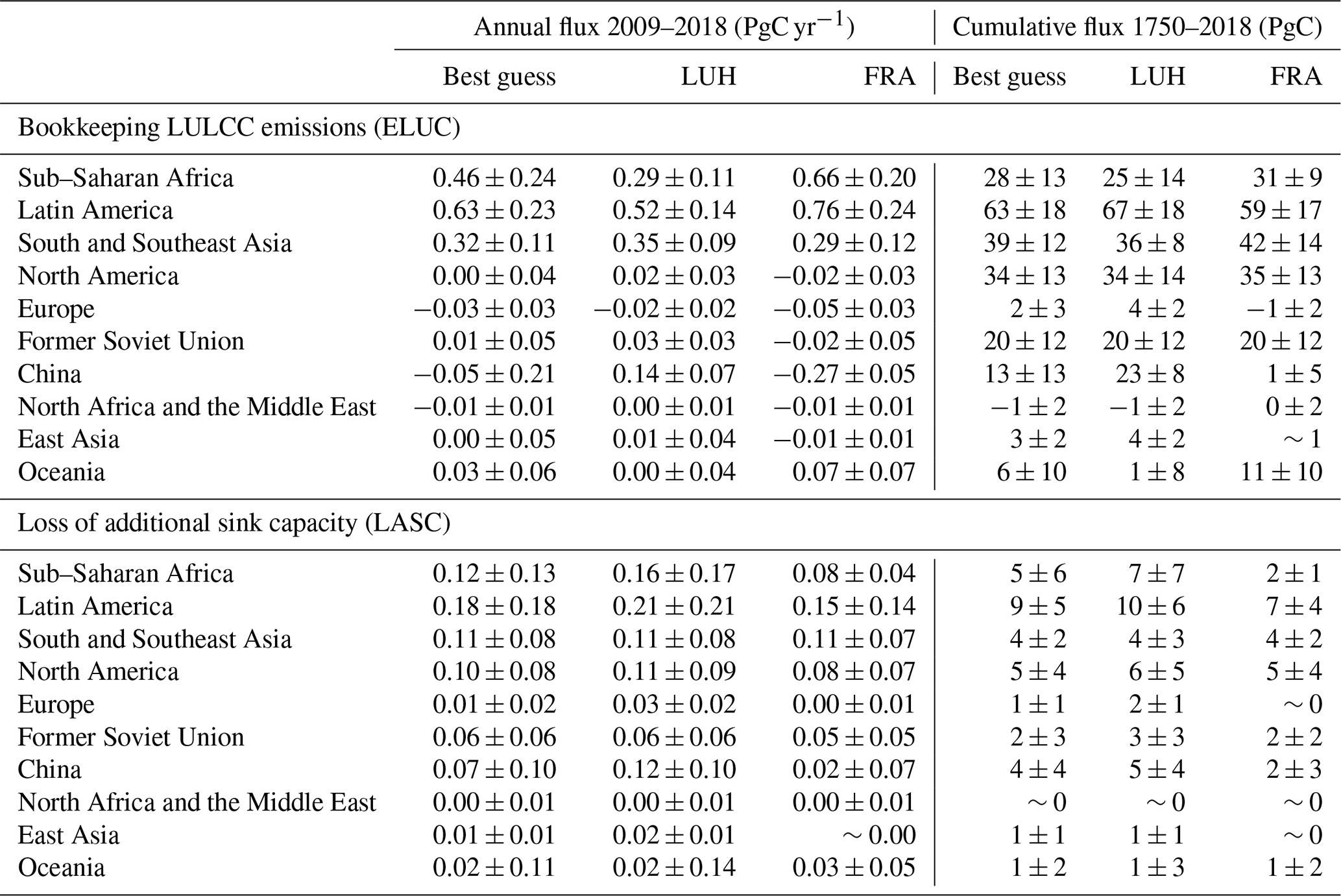
Table 4Regional breakdown of bookkeeping LULCC emissions and LASC. This is provided for our best-guess estimates and the two main LULCC data sets (LUH2-GCB2019 and FRA2015) separately. The regions are defined in Houghton and Nassikas (2017).
3.4 Breakdown by region
Figure 4 and Table 4 provide our best-guess estimates of the bookkeeping LULCC emissions in our 10 broad world regions. Unsurprisingly, tropical regions (Latin America, sub-Saharan Africa, and South and Southeast Asia, in decreasing order) are found to be the main LULCC emitters over the last decade, with a positive trend over the last 50 years. Conversely, North America, Europe, the former Soviet Union, and China are all found to have a decreasing trend over the last 50 years – to the point of North America, Europe, and China being net carbon absorbers over the last decade. Looking at a larger historical period, Latin America and South and Southeast Asia were the top two emitters over the 1750–2018 period, with North America being the third-highest emitter. It must be noted, however, that this ranking is not statistically significant due to uncertainties. When the subset of our simulations driven by the FRA2015 data set is isolated, our estimates compare very well to the estimates of H&N (Houghton and Nassikas, 2017; see Table A3 in Appendix).
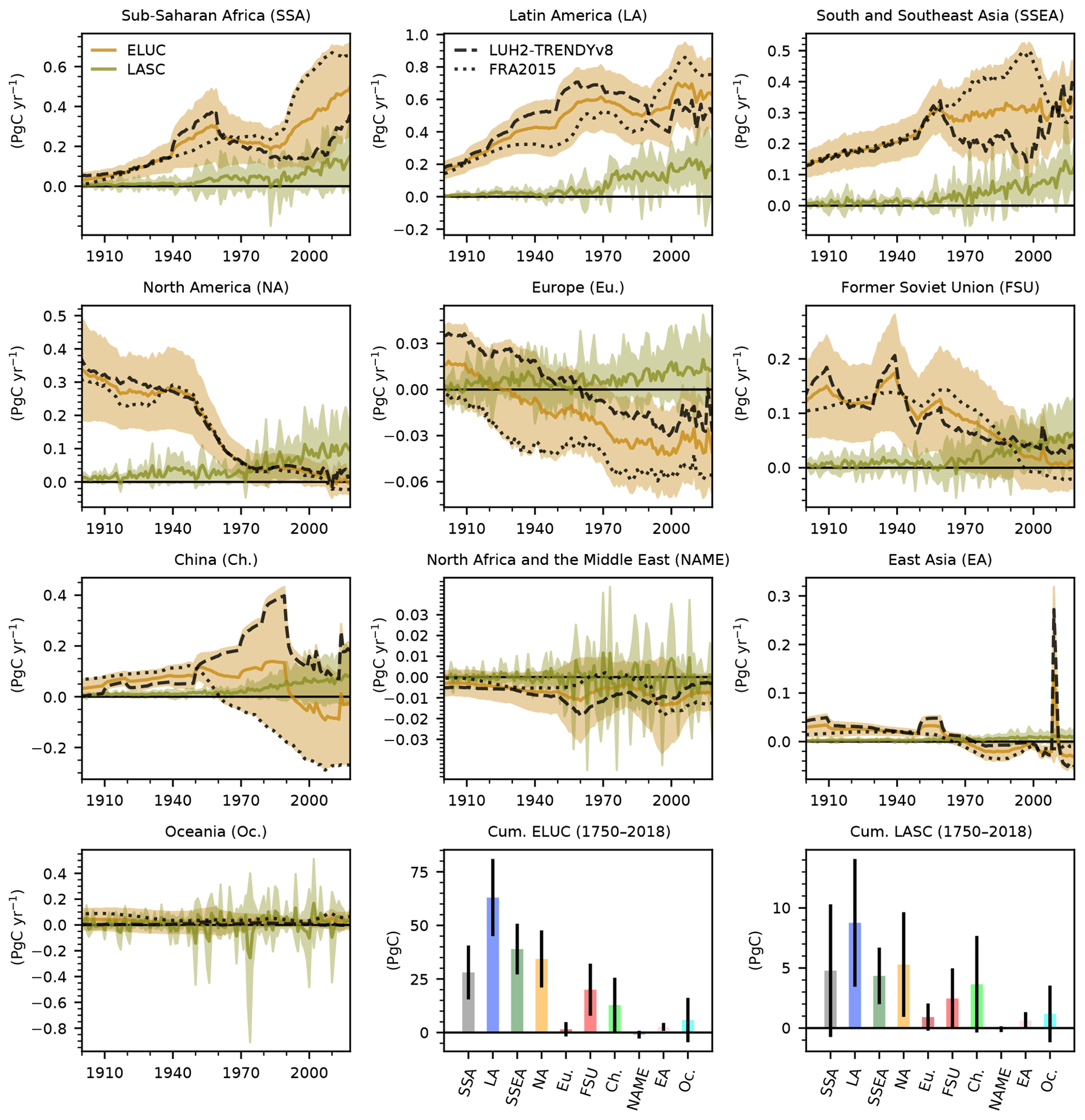
Figure 4Regional breakdown of our best-guess estimates. Annual bookkeeping LULCC emissions (in brown) and LASC (in green) are shown, except in the last two panels where the regional cumulative bookkeeping LULCC emissions (ELUC) and LASC over the 1750–2018 period are shown. Shaded areas and uncertainty bars represent the 1σ uncertainty range. To help identify regional discrepancies between LULCC driving data sets, we also separate the average estimates for the LUH2-GCB2019 (dashed black line) and FRA2015 (dotted black line) data sets (which are shown without their own uncertainty for legibility).
The uncertainty in our regional bookkeeping LULCC emissions can be attributed to the LULCC data sets and the biogeochemical parameters using Fig. 4 and Table 4. For North America, the former Soviet Union, and, to a lesser extent, Europe, the two LULCC data sets lead to emissions that are in rather good agreement; this implies that the regional uncertainty is dominated by the biogeochemical parameterization. In tropical regions, however, the two data sets show substantial disagreement – to the point of being the main source of uncertainty in sub-Saharan Africa and in South and Southeast Asia. Remarkably, the disagreement in the emissions of Latin America is shown in Fig. 4, but the inverse global trends is shown in Fig.3b. China is another region in which the discrepancy between the two data sets leads to a substantial uncertainty range. On the one hand, FRA2015 exhibits large-scale forest plantation in China based on national declarations, which leads to a significant atmospheric carbon removal; on the other hand, the LUH2-GCB2019 ignores those declarations and considers that China lost a large amount of forest over the same period. Ultimately, it is not the goal of this paper to provide a detailed analysis of the regional discrepancies between the two data sets nor to recommend one over the other. Nevertheless, we produced Fig. A2, which shows regional LULCC drivers, to offer a starting point for such an endeavor.
Our estimate of the LASC is also broken down regionally in Fig. 4. The annual LASC of most regions follows a similar trend to the global one. However, in North Africa and the Middle East as well as in Oceania, the noise produced by the inter-annual variability appears to dominate over the trend. It is unclear what exactly causes this noise, but the fact that both regions include large non-vegetated areas suggests that the parameterization of OSCAR is not very robust in such a case. The noise intensity in Oceania is even larger than the signal in any other region, suggesting that some of the uncertainty in our LASC estimates could be an artifact of this weakness in our modeling approach. As to the regional split of the cumulative LASC over the 1750–2018 period, it roughly follows that of the cumulative LULCC emissions, although it is modulated by the land sink's relative efficiency in each region. Latin America is the region in which the largest part of this loss of sink capacity occurred (almost one-third), followed by North America, South and Southeast Asia, and sub-Saharan Africa. However, uncertainties in the LASC are too high for this ranking to be determined with good statistical confidence.
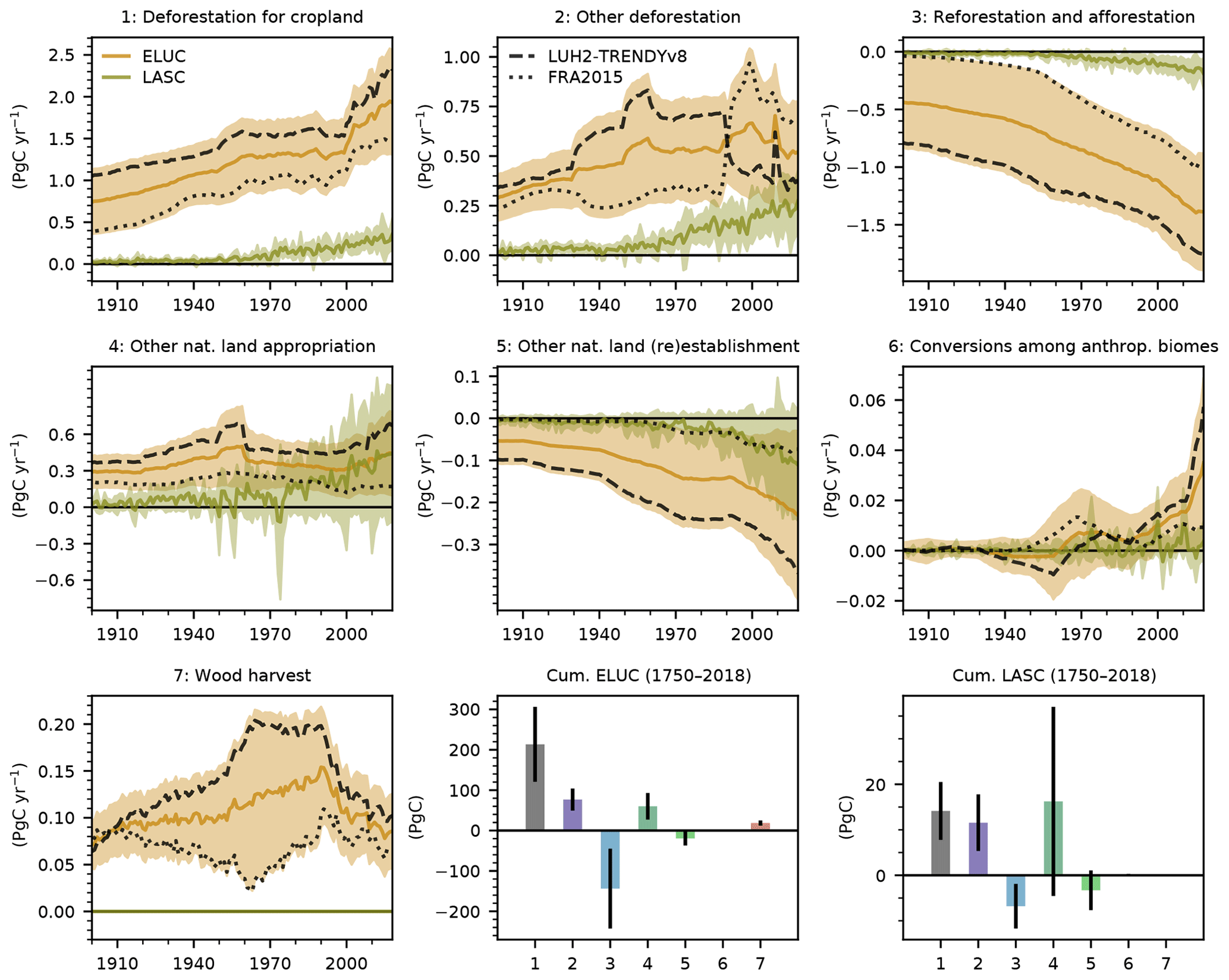
Figure 5Breakdown of our best-guess estimates by LULCC activities. Annual bookkeeping LULCC emissions (in brown) and LASC (in green) are shown, except in the last two panels that show the regional cumulative bookkeeping LULCC emissions (ELUC) and LASC over the 1750–2018 period. Shaded areas and uncertainty bars represent the 1σ uncertainty range. Similarly to Fig. 3, we also separate the average estimates for the LUH2-GCB2019 (dashed black line) and FRA2015 (dotted black line) data sets (which are shown without their own uncertainty for legibility).
Table 5Breakdown of bookkeeping LULCC emissions and LASC by LULCC activity. This is provided for our best-guess estimates and the two main LULCC data sets (LUH2-GCB2019 and FRA2015) separately.
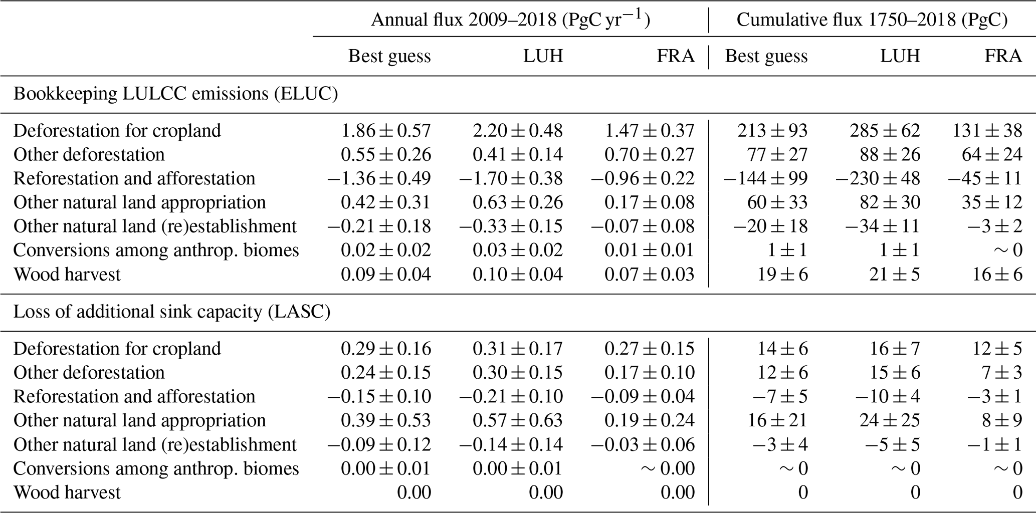
3.5 Breakdown by transition
Figure 5 and Table 5 show a breakdown of our global bookkeeping LULCC emissions and LASC following seven categories of LULCC activities. These categories are essentially a subdivision of the main three LULCC activities mentioned previously in the short description of OSCAR. Category 1 corresponds to land cover change (LCC) where forest is replaced by cropland. Category 2 is LCC where forest is replaced by anything else (but forest). Category 3 is the opposite of 1 and 2: LCC where any type of land but forest is replaced by forest. Category 4 is LCC where non-forested natural land is replaced by any anthropogenic land. Category 5 is the opposite of 4. Category 6 is any LCC occurring among anthropogenic land (e.g., pasture to cropland). Category 7 is the sum of wood harvest and LCC occurring from any type of natural land to the same type of natural land (e.g., forest to forest). Note that the effects of shifting cultivation are included in their corresponding LCC categories due to the model's structure.
Forest-related land cover change dominates historical bookkeeping emissions. Over the last decade, we estimate that an average of 1.86±0.57 PgC yr−1 was emitted due to deforestation in order to establish cropland, an additional 0.55±0.26 PgC yr−1 was from other types of deforestation (e.g., deforestation for pastoral land or simply due to forest degradation), and a capture of PgC yr−1 was due to reforestation and afforestation. These estimates include the effect of our shifting cultivation driver that encompasses traditional activities such as “slash-and-burn”, which leads to large but counteracting gross carbon fluxes caused by back-and-forth deforestation/reforestation activities (Houghton et al., 2012; Li et al., 2018; Yue et al., 2018). The cumulative emission over the 1750–2018 period was 213±93 PgC due to deforestation for cropland, 77±27 PgC due to other types of deforestation, and 60±33 PgC due to the loss of other natural land. This was partly compensated for by PgC from reforestation and afforestation as well as PgC when other natural land was regained.
The uncertainty in the bookkeeping LULCC emissions is largely dominated by the discrepancy between the two main LULCC data sets. For annual emissions, this is even reinforced by the fact that shifting cultivation is included in our estimates. Figure A2 indeed shows that both data sets have a very different level of shifting cultivation area, although this is somewhat artificial as it is caused by the difference in the data sets' starting year. Therefore, our uncertainty ranges for the deforestation and reforestation categories are overestimated. For cumulative emissions, however, this overestimation is much lower, as shifting cultivation has a long-term effect of zero net emissions in OSCAR (Appendix A7). However, a few other clear differences between the two data sets remain, such as the opposite trend in 1990 in the “other deforestation” category or the difference in wood harvest.
When we split the LASC between these transitions types, we obtain a slightly different picture. Our three categories of natural land appropriation caused roughly similar amounts of cumulative LASC: 14±6 PgC from deforestation for cropland, 15±6 PgC from other deforestation, and 24±25 PgC from loss of other natural land. This was partially compensated for by a negative LASC (i.e., an increase in the sink capacity) of PgC caused by reforestation and afforestation and PgC caused by other natural land gain. Other types of LULCC led to a negligible LASC. Regarding the uncertainty in the LASC, the noise we identified in the previous section can be attributed to the “other natural land” biome. Combined with the diagnosis from the previous section, this suggests that OSCAR may benefit from separating desert areas (i.e., bare soils) from the non-forest biome. However, this would make processing the LULCC data sets more difficult, as new assumptions should then be made regarding how much of this new biome is affected by LULCC.
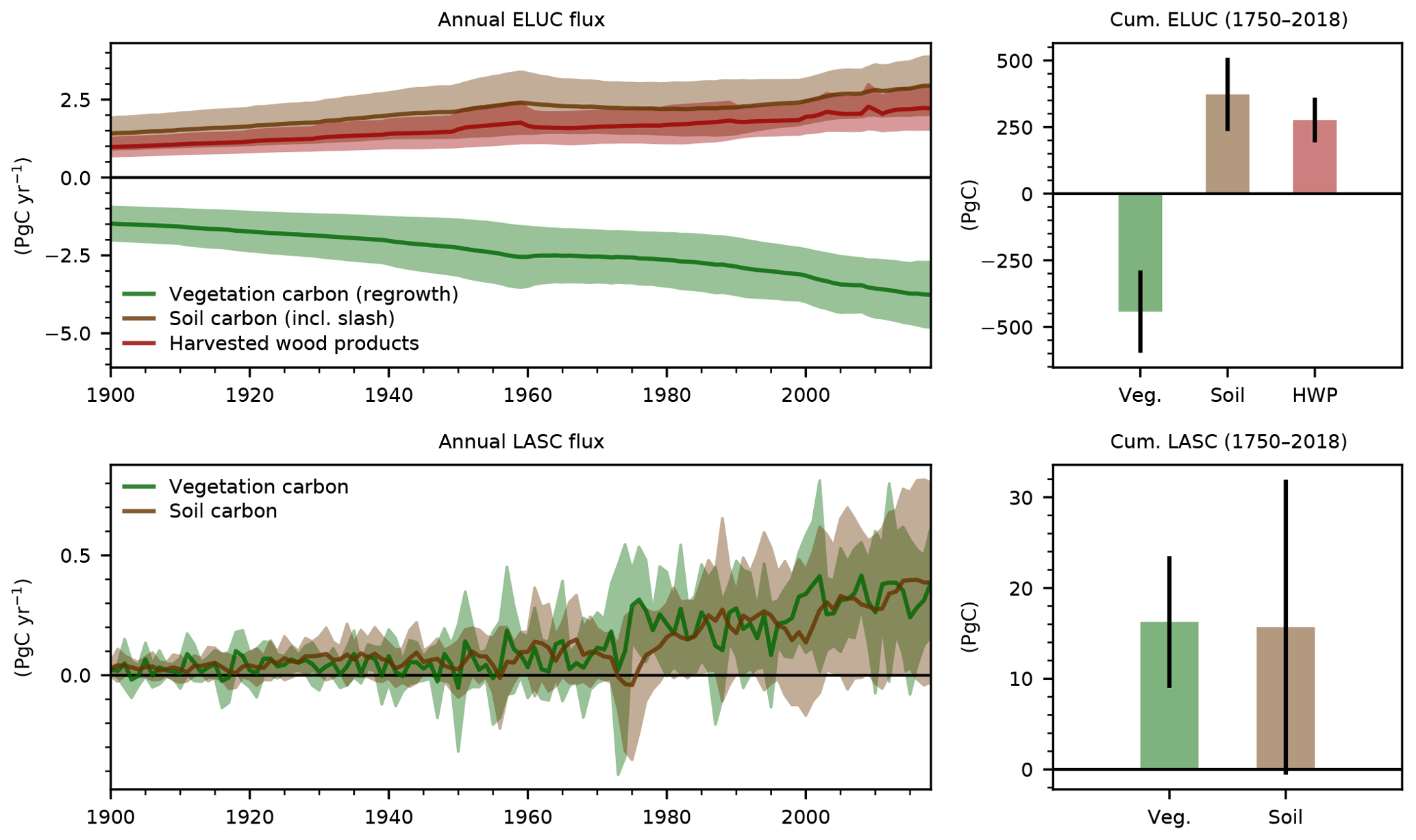
Figure 6Breakdown of our best-guess estimates by carbon pools: vegetation (green), soils (brown), and HWPs (red). Shaded areas and uncertainty bars represent the 1σ uncertainty range.
3.6 Breakdown by carbon pool
A final axis of analysis that OSCAR can provide is a breakdown of the model's carbon pools, thereby indirectly following its biogeochemical processes. Figure 6 shows such a breakdown into our three main carbon pools: vegetation carbon, soil carbon, and HWPs. Bookkeeping LULCC emissions over the last decade have consisted of a combination of PgC yr−1 of vegetation carbon (i.e., biomass) regrowth, 2.84±0.85 PgC yr−1 emitted by equilibrating soils, and 2.18±0.65 PgC yr−1 emitted by HWP oxidization. Here, the equilibration of soils includes both the heterotrophic respiration in originally carbon-rich soils that is not compensated for by enough primary productivity (e.g., when deforesting to establish cropland) and the oxidation of slash products (i.e., dead biomass left on site after land cover change). The three sub-fluxes have been steadily increasing over the past century or so. Cumulated over the 1750–2018 period, these three pool-specific values amount to , 373±137, and 276±84 PgC, respectively.
For the LASC, this pool-based decomposition only concerns the vegetation and soil pools, as no HWPs are involved in the processes driving the land sink. Both components of the annual LASC are positive, with notable inter-annual variability and positive trend, reaching 0.33±0.25 PgC yr−1 for the vegetation and 0.35±0.36 PgC yr−1 for soils, on average over the 2009–2018 period. Over the 1750–2018 period, the cumulative component fluxes are 16±7 PgC for vegetation and 16±16 PgC for soils. These positive values must be interpreted as a storage of carbon that did not occur because the preindustrial land cover was modified and the new ecosystems could not provide as strong a land sink as the preindustrial ecosystems. The breakdown shows how this storage would have been split between vegetation and soil carbon pools, had it occurred. Since it is implicitly determined by the model's processes, this breakdown is heavily model dependent and is largely dominated by the biogeochemical uncertainty.
4.1 The constraint
Table 2 shows that the choice of constraint does not drastically impact our results, as there is a large overlap between the estimates obtained with both the old and new constraints. More precisely, LULCC emissions do not show a large impact, whereas the land sink and the LASC do. However, this is somewhat artificial, as both our constraints are aimed at constraining the processes that dictate the land sink (such as the fertilization effect), which is visible in Fig. 1c where the unconstrained distribution of the land sink exhibits a large spread that is reduced after the application of constraints. Other (or additional) constraints focused on LULCC emissions, such as constraints on carbon densities, could be envisioned – although we deemed this unnecessary for this study. Because the constraint is applied after the simulations are actually run, it is indeed possible to decide on the best constraint (or combination thereof) ex post, depending on one's ultimate goal. Our choice of constraint was driven by our will to make our estimates of LULCC emissions compatible with the overall GCB2019, our scientific conviction that it is preferable to use physical (i.e., observable) variables as constraints, and our own expert judgement as to which parts of the GCB are the most robust. Our choice can be debated, however, and we invite the community to download our raw estimates and apply their own constraints if they so wish (see the “Data availability” section). Ultimately, a Bayesian synthesis framework could be used at the GCB scale (Li et al., 2016) to avoid having to make such an arbitrary choice.
4.2 The OSCAR model
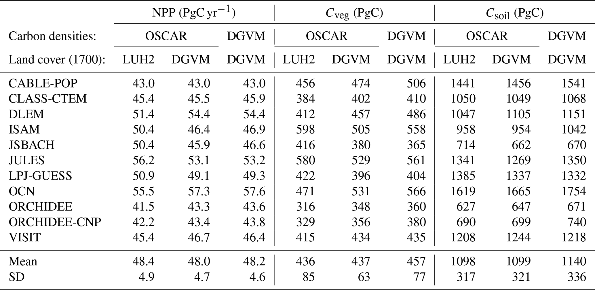
OSCAR satisfactorily emulates the carbon densities and stocks of DGVMs (Table A1), but these stocks are in the lower end of existing assessments. The DGVMs we calibrated OSCAR upon have global preindustrial pools of 457±77 PgC for vegetation and 1140±336 PgC for soil, whereas the IPCC Fifth Assessment Report (Ciais et al., 2013) gives values of 450–650 and 1500–2400 PgC, respectively. Some of the difference in soil carbon comes from the absence of peatland in DGVMs (Nichols and Peteet, 2019), and some may be explained by the existence of “passive” soil carbon that is not mobilized under the timescales we consider here (Barré et al., 2010; He et al., 2016). Nevertheless, the relatively low carbon pools suggest that our bookkeeping LULCC emissions could be underestimated. Alternatively, our preindustrial land cover taken from the LULCC data sets could be inaccurate (Table A2). We ran the LUH2 data set starting in 850, and did not find substantial carbon loss between 850 and 1750 (23±15 PgC in total). Other studies that specifically focused on the more distant past have found much higher carbon loss over this early period (Erb et al., 2018; Kaplan et al., 2011; Pongratz et al., 2008), again suggesting this part of our results could be underestimated.
A key feature of OSCAR is that the model's carbon densities transiently change as a response to changes in environmental conditions. This change in carbon densities is fully coupled to the bookkeeping module and, therefore, impacts bookkeeping LULCC emissions. This feature contrasts with the fixed carbon densities of other bookkeeping models and makes it possible to account for processes such as CO2 fertilization, wildfire changes, and climate feedbacks. Without any change in environmental conditions, we find that annual bookkeeping LULCC emissions would have been 1.11±0.35 PgC yr−1 on average over the last decade, and cumulative emissions would have been 191±52 PgC over the 1750–2018 period. This is 19 % and 7 % less than our best guesses with environmental changes for the abovementioned periods, respectively, and is primarily driven by the lower carbon densities that are caused by the absence of the fertilization effect. The effect on the cumulative emissions is in line with a previous estimate (Gasser and Ciais, 2013). The effect on annual emissions, however, is higher. This suggests that this effect increases with time and will keep increasing in the future as environmental conditions change and move further away from preindustrial conditions. This underscores the importance of building hybrid bookkeeping models such as OSCAR that are capable of capturing such an effect. A structural limitation of this version of OSCAR is the absence of any age-specific process. This means that none of the model's parameters depend on the time elapsed since a given LULCC perturbation (i.e., it has no age classes). For instance, 5-year-old forests grow and die at the same rate as 50-year-old forests. This, by construction, means that the biomass regrowth of disturbed ecosystems follows an exponential response curve, which we acknowledge is unrealistic. The impact of this structural choice is difficult to estimate; however, as it affects only dynamics and not carbon densities, we can speculate that annual emissions are more impacted than cumulative emissions. Other regrowth curves could be introduced (Fekedulegn et al., 1999), although this would require the introduction of age-dependent functions in the model's formulation, which, in turn, would make it heavier and slower. Actually, when OSCAR v2.4 was developed, the only process that had been age dependent until then, namely the decay of HWPs (Gasser et al., 2017), was reformulated to be age independent. The reason for this simplification is that, beyond being a carbon cycle model, OSCAR is also an Earth system model, and the complexity of each of its modules has to be kept in check. However, it is not excluded that future variants of the model will see implementation of such a feature.
A final structural element that we find worth mentioning is the biome aggregation of our model. The final list of five biomes in OSCAR is a trade-off between the plant functional types (PFTs) of the DGVMs and the land cover classes of the LULCC data sets. Typically, DGVMs tend to focus on natural ecosystems (i.e., they have many types of forests), whereas LULCC data sets focus on anthropogenic ecosystems (i.e., more types of croplands and pastures). Our list of biomes aimed at limiting the number of assumptions made when processing both types of data for implementation within OSCAR, but some were necessary nonetheless. Qualitatively, we see two important caveats caused by our biome aggregation. First, as we only have one natural biome to cover all natural land but forests, we average actual natural ecosystems with relatively high carbon densities such as shrubland with almost carbon-free ecosystems like deserts. We saw in previous sections that this may explain part of the large uncertainty in our LASC estimates, but it likely also affects our bookkeeping LULCC emissions. Second, we do not distinguish between primary and secondary natural land. In other words, pristine and disturbed natural ecosystems are assumed to have the same steady-state carbon densities. However, this does not mean that the actual carbon densities are the same. It means that it is assumed that, if left undisturbed, previously disturbed ecosystems will grow back to the exact same steady state as those that have never been disturbed. Because they relate to carbon densities, these structural aspects are likely to have the largest impact on our estimates. Quantifying this impact would require a significant amount of work; however, it would undoubtedly require making new assumptions that, in turn, would introduce additional uncertainty and potential biases.
In spite of those caveats, this study has introduced an innovative method to estimate historical LULCC emissions and LASC, whereby a bookkeeping approach, data from processed-based models, several LULCC data sets, and an empirical constraint are consistently combined. We have also identified key sources of uncertainty that must be reduced to improve future GCBs. One easy improvement is to decide on where to account for the LASC. We argued elsewhere (Gasser and Ciais, 2013) that it is ill-advised to include the LASC in LULCC emissions, as it is a theoretical flux that cannot be observed and that does not tend to zero after LULCC activities cease. However, reducing the other sources of uncertainty is a more challenging endeavor. Although satellite data (Hansen et al., 2013) and crowd-sourcing (Fritz et al., 2019) are currently promising ways of establishing more accurate land cover maps, these must be backcast over the past to be relevant for the long-term dynamic of the global carbon cycle. Such backcasting generates new uncertainty (Peng et al., 2017), and additional data, perhaps in the form of historical records (Bastos et al., 2017; Houghton and Nassikas, 2017), are required to mitigate the lack of direct observations. We found that the biogeochemical uncertainty dominated, although that is a reflection of the uncertainty in the DGVMs' own parameterization, and not the uncertainty stemming from direct observations of real-life carbon densities. Improving the DGVMs' calibration (e.g., by assimilating observational data) is an obvious albeit resource-intensive way of reducing this source of uncertainty. Posterior evaluation and weighting of the DGVMs is another approach, be it through a specifically designed protocol such as the International Land Model Benchmarking (ILAMB) project (Collier et al., 2018) or a synthesis setup like ours.
A1 A brief description of the land carbon cycle module
The land carbon cycle module of OSCAR v3.1 is used in “offline” mode: it is not coupled to the rest of the Earth system and, in particular, permafrost carbon release (Gasser et al., 2018) is not accounted for. The global terrestrial biosphere is divided into pairs of regions and biomes, noted (i, b), representing the “average” biome b of the ith region with assumed homogeneous biogeochemical characteristics. Therefore, the module is not spatially explicit, and the regional aggregation for this study follows the 10 regions defined in Houghton and Nassikas (2017; their Table 2) and 5 biomes (forests, other natural lands, croplands, pastures, and urban lands). A detailed analytical description of the module is provided in Appendix A7.
The first part of the module describes the evolution of vegetation, litter, and soil carbon densities (i.e., carbon stocks per unit area) as well as the areal carbon exchanges between these pools and/or the atmosphere, within each set (i, b) and in the absence of LULCC. The preindustrial steady-state values of these carbon densities and areal fluxes are calibrated on DGVMs. During a transient simulation, these values are affected by environmental conditions: changes in atmospheric CO2 concentration impact net primary productivity (NPP) – the “fertilization” effect – and wildfire intensity, while changes in regional yearly temperature and precipitation alter NPP, wildfire intensity, and heterotrophic respiration rate.
Table A1Preindustrial NPP and carbon stocks in GCB2018 DGVMs and in their emulation by OSCAR. The “DGVM” columns show the carbon fluxes or stocks we extracted for the calibration of OSCAR. Because we used our own land area map and regional mask to process the original DGVM outputs and then aggregated regional values into global values, these values may slightly differ from a direct extraction of the DGVM outputs. The GCB2018 protocol did not require the DGVM teams to provide their own land area map.
The second part of the module describes the effect of LULCC using a bookkeeping approach. When a LULCC perturbation occurs, carbon from the originally undisturbed (i, b) pools is redistributed to other pools, including an anthropogenic pool of harvested wood products (HWPs). The new pools can also be within another biome b′ in the case of land cover change. This displaced carbon follows the biogeochemical properties of the new pools, thereby slowly tending toward a new steady state. Following the discussion and recommendation of Gasser and Ciais (2013), the carbon fluxes and pools of these transitioning ecosystems are defined as a difference to their expected but yet to be reached new steady state; thus, the effect of any LULCC perturbation tends toward zero in the long run. This bookkeeping approach corresponds to “definition 3” introduced by Gasser and Ciais (2013) and to “definition B” of Pongratz et al. (2014).
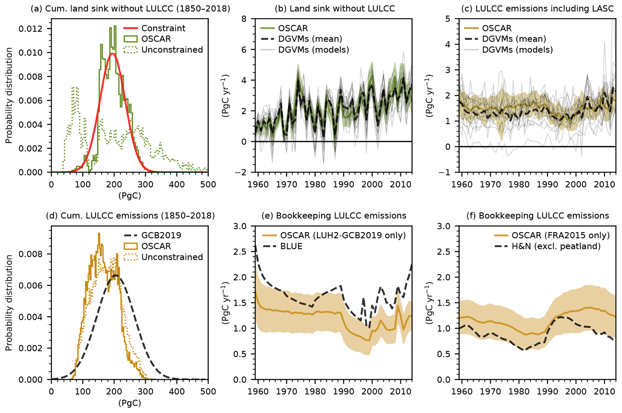
Figure A1The effect of the alternative constraint and comparison to the GCB2019. (a) Probability distributions in the unconstrained (dotted histograms) and constrained (plain histograms) OSCAR ensembles of the cumulative terrestrial carbon sink over the 1850–2018 period in the absence of LULCC perturbation compared with the constraint (red). (b) The annual terrestrial carbon sink in the absence of the LULCC perturbation simulated by OSCAR (color), the individual GCB DGVMs (light gray), and their multi-model mean (dashed black). (c) The annual LULCC emissions deduced from the GCB DGVMs (i.e., including the LASC). (d) Probability distributions of our best-guess estimate of the cumulative LULCC emissions over the 1850–2018 period compared with the GCB estimate (dashed black). (e) Bookkeeping LULCC emissions when the model is driven by the LUH2-GCB2019 data set compared with BLUE estimates reported by the GCB2019. (f) Bookkeeping LULCC emissions when the model is driven by the FRA2015 data set compared with H&N estimates from which emissions from peatlands were subtracted. All shaded areas show the 1σ uncertainty range.
A2 Recalibration of the preindustrial land carbon cycle
The carbon cycle in each combination of region and biome (i, b) is represented by a three-box model, illustrated in Fig. A3. In OSCAR v3.1, the three-box model was slightly altered but remains very close to that of earlier versions (Gasser et al., 2017). Concretely, a flux going directly from the vegetation carbon pool to the soil carbon pool (and therefore bypassing the litter carbon pool) was added (“fmort2” in Fig. A3). This simple change enables one to use the three-box model as a two-box model without changing its structure or equations. In turn, this enables complex models that do not provide enough information to be emulated with a two-box model but using the three-box model's equations. In addition to this increased flexibility, the model was extended using two new fluxes: emissions from harvested crop products (“eharv”) and emissions caused by pasture grazing (“egraz”).
Table A2Global preindustrial (1700) land cover (in Mha) in the GCB2018 DGVMs compared with that from our two main LULCC data sets.

In OSCAR v3.1, the parameters describing the preindustrial steady state of the land carbon cycle module were recalibrated on outputs of the DGVMs that took part in the GCB2018 (Le Quéré et al., 2018a), i.e., the TRENDYv7 models. We used outputs from the control experiment (named “S0” in their protocol), in which no LULCC occurs and environmental conditions such as atmospheric CO2 and climate are maintained at their preindustrial level, to calibrate the parameters of the natural biomes (“forest” and “non-forest”). However, because it follows preindustrial (here, 1700) land cover data, the areal extent of anthropogenic biomes (“cropland”, “pasture”, and “urban”) is very low in the S0 experiment. For these anthropogenic biomes, in order to avoid any bias in their parameters potentially caused by this low land cover fraction, we decided to use the last years of another experiment instead (namely, “S4”), in which historical LULCC occurs but environmental conditions are still maintained at preindustrial levels. We acknowledge that the existence of LULCC in S4 is not in line with our aim of calibrating a steady state, but it is a necessary compromise in order to have a large enough areal extent of anthropogenic biomes for proper calibration. Note that some DGVMs did not provide enough data and could, therefore, not be used for calibration at all, which led to a total of 11 models used out of the 16 original DGVMs (see Table 1). A detailed calibration protocol is given in Appendix A8.

Figure A2Summary of LULCC drivers in LUH2-GCB2019 (dashed black lines) and FRA2015 (dotted gray lines). For each region (rows), the first five columns show net changes in our five biomes (in order: forest, non-forest, cropland, pasture, and urban), the second-to-last column shows wood harvest, and the final column shows total area under shifting cultivation.
Table A1 shows a comparison of the global net primary productivity and carbon pools in the OSCAR v3.1 and in the original DGVMs. The emulation is not perfect, and the preindustrial global (and regional) carbon pools of OSCAR do not exactly match those of the emulated DGVMs. There are three main reasons for this. First, since we average and homogenize biogeochemical properties over large world regions, we lose some accuracy, as unevenly distributed carbon pools are not explicitly represented in OSCAR. This bias is somewhat reduced by defining regions that show a certain bioclimatic consistency (e.g., separated tropical regions). Second, OSCAR works with clearly defined biomes; therefore, we have to map the DGVMs' plant functional types (PFTs) onto the biomes of our model. Since few DGVMs provide detailed fluxes and pools on a PFT basis, we further have to use an ad hoc method to distribute aggregated variables between our biomes (see the detailed calibration protocol). Third, we calibrate carbon densities and not stocks, and some discrepancy is introduced by the fact that we do not use the DGVMs' preindustrial land cover map (Table A2). Despite these three caveats, Table A1 demonstrates that the emulation remains largely satisfactory.
A3 Changes between OSCAR v2.2 and v3.1
The following points outline the changes between OSCAR v2.2 and v3.1:
-
v3.1. Changes to the land carbon cycle are described hereinabove (Appendix A2). The new structure made it necessary to adapt the wetlands module, so that CH4 emissions from wetlands now scale with the relative change in total heterotrophic respiration (and not the change in litter respiration).
-
v3.0.1. An error in the overlap function for the radiative forcing of CH4 and N2O was corrected. This error appeared during the rewriting of v3.0 and did not affect earlier versions.
-
v3.0. OSCARv3 was completely recoded from scratch in Python 3 (instead of Python 2), with an entirely new structure and solving scheme. This version heavily relies on the “xarray” Python library (Hoyer and Hamman, 2017) to parallelize Monte Carlo simulations and/or scenarios. The default solving scheme was changed to a forward-Eulerian exponential integrator. All underpinning physical equations and parameter values remain the same as in v2.4. Both versions were compared, and no significant difference was found beyond the effect of the new solving scheme.
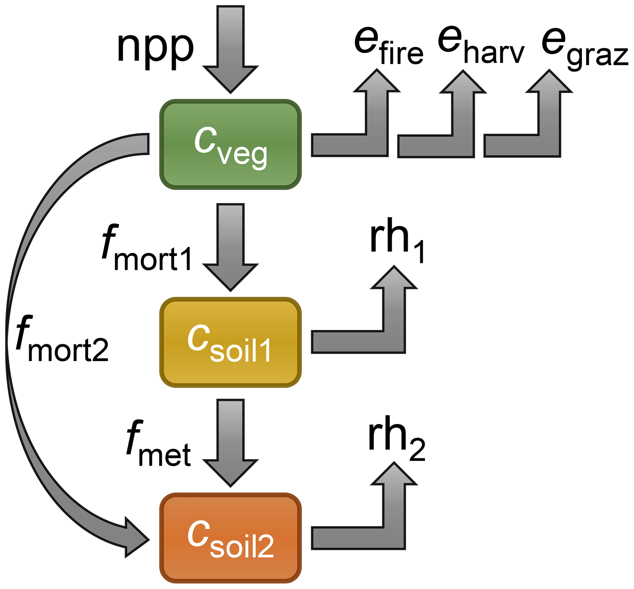
Figure A3Diagram of the three-box model describing the intensive land carbon cycle in each (region, biome) set. The three boxes correspond to carbon pools in the vegetation (cveg), the litter (csoil1), and the soil (csoil2). Detailed definitions and formulations of the fluxes (gray arrows) are provided in Appendix A7.
-
v2.4. This version was developed as a bridge version between v2 and v3. Our goal was that v2.4 be as close to v3.0 as possible (without changing the overall structure of the model) at this point. The preindustrial land cover map was changed to being that of the LULCC data set used to drive the model. The dependency of the fractional area of wetlands to the preindustrial land cover map was removed and was taken as the average of all previous parameterizations. The possibility of having HWPs follow a non-exponential decay was removed. To compensate for this, in addition to the original parameterization of the HWP lifetimes (called “normal”), two new options were added in which these lifetimes are rescaled by 0.5 (“fast”) or by 1.25 (“slow”). Finally, the biome aggregation was fixed to that of v3: the five biomes described in this paper.
-
v2.3.1. A number of minor errors were fixed, and additional adjustments were made. Land carbon cycle parameters for the urban biome were corrected. So were one parameterization for the radiative efficiency of tropospheric O3 and one parameterization for the semi-direct effect of black carbon (BC) aerosols. One parameterization for the effect of N2O on stratospheric O3 and one parameterization for the fractional release factor of ozone-depleting substances were removed. One parameterization for the radiative efficiency of tropospheric O3 was added. All of these changes had almost no impact on the model's performance. However, two additional changes had more impact: first, the discretization of the response functions for HWPs was corrected, which led to higher LULCC emissions after correction; and, second, a new parameter was introduced to account for the fact that too much of the HWPs were assumed to be burned. This amount was reduced by half, leading to better endogenous non-CO2 biomass burning emissions but having no impact on the CO2 budget.
-
v2.3. The permafrost carbon model described by Gasser et al. (2018) was implemented in the model's main branch.
-
v2.2.2. A minor error in one parameterization for the lifetimes of primary organic aerosols (POAs) and BC was fixed. This had very little impact on the overall performance of the model.
-
v2.2.1. Two errors in the code were fixed. The first was in the function linking the surface ocean carbon pool to the surface ocean partial pressure in CO2, which was leading to an overly efficient ocean carbon sink under high warming and high atmospheric CO2. However, the effect was negligible under historical conditions. The second was in the function linking atmospheric CO2 and surface ocean pH change. This function was not described by Gasser et al. (2017); it was taken from Bernie et al. (2010) but was incorrectly implemented.
-
v2.2. This version was comprehensively described by Gasser et al. (2017).
Table A3Comparison of regional bookkeeping LULCC emissions with H&N estimates. H&N values are taken directly from Houghton and Nassikas (2017): their annual flux is calculated over the 2006–2015 period, and their cumulative flux is calculated over the 1850–2015 period.

A4 Experimental setup
The land carbon cycle module of OSCAR is driven by (i) global atmospheric CO2 concentrations over the 1700–2018 period created for the GCB2019 exercise (Friedlingstein et al., 2019), (ii) observation-based reconstructions of regional air temperature and precipitation over the 1901–2018 period from the CRU-TS v4.03 (Harris et al., 2014), and (iii) several LULCC data sets detailed hereafter. Atmospheric CO2 before 1700 is assumed to be constant and equal to the preindustrial value used in OSCAR (Gasser et al., 2017), which is a very slight deviation from the GCB protocol, as our model's preindustrial reference year is 1750 and not 1700. Climate variables are offset by their average over the 1901–1920 period, assuming that this corresponds to a preindustrial climate that is further extended backward before 1901. This is similar to the GCB protocol with the exception of the fact that we use the average of 1901–1930, whereas the GCB recycles the individual years of this period (leading to a 30-year cycle). This difference was tested, and we found only a negligible effect on our results (not shown).
Our best-guess estimates are based on two significantly differing LULCC data sets. The first one is an update of the LUH2 data set made for the GCB2019 exercise, in which only the years after 1950 differ slightly from the original data set. The second one is the data set used and created by Houghton and Nassikas (2017) on the basis of FAO and FRA2015 data. Although these two data sets have several data sources in common, they remain mostly independent given the way that they internally process these input data. Additionally, for Fig. 3, we ran simulations with older variants of the LUH data set. These variants are as follows: the first Land-Use Harmonization (LUH1) data set (Hurtt et al., 2011), originally produced for the CMIP5 modeling exercise; an updated version of LUH1 made for the GCB2015 exercise, which was based on then-preliminary HYDE3.2 data (Klein Goldewijk et al., 2017) instead of HYDE3.1 data (Klein Goldewijk et al., 2011); and the original LUH2 data set produced for CMIP6, as well as its two “Low” and “High” variants (Lawrence et al., 2016). All of these data sets required some slight processing, as described in Appendix A9. Our simulations start in the earliest year of the LULCC data sets: in 850 for LUH2 variants, in 1500 for LUH1 variants, and in 1700 for FRA2015. This significantly differs from the GCB protocol that starts in 1700.
A5 Constrained Monte Carlo ensemble
All of those simulations were made following a probabilistic Monte Carlo setup in which 10 000 sets of the model's parameters were drawn randomly (with equiprobability). Note that these parameters include the nine parameters introduced in Appendix A7 (multiplied by the number of (i, b) pairs) as well as additional parameters described by Gasser et al. (2017) for a total of more than 1300 parameters. The combination of Monte Carlo elements, LULCC data sets, and variant runs led to a total of 140 000 simulations and about 100 million simulated years. We constrained this large ensemble to limit the bias and spread that typically results from using OSCAR in such a probabilistic fashion (Gasser et al., 2017). This is done in a way similar to what we did for the GCB2017 (Le Quéré et al., 2018b). Each element of the Monte Carlo ensemble is given a weight (w) equal to
where μ and σ are the mean and standard deviation of the constraint, respectively, and x is the value of the corresponding variable for this element of the ensemble. The constraint we use in this study is the cumulative net land-to-atmosphere flux over the 1850–2018 period, calculated as the residual of the carbon emitted by fossil fuel burning and industry minus the carbon stored in the atmosphere and the ocean. These values were taken from the GCB2019 (Friedlingstein et al., 2019; their Table 8), leading to and σ=30 PgC. See Fig. 1 and Sect. 4 in the paper for more on the effect of the constraint.
A6 Debiased uncertainty
To analyze and separate each uncertainty factor, we average our simulations ensemble over all uncertainty axes except the one investigated and then quantify the absolute (standard deviation) and relative (coefficient of variation; CV) uncertainty along the remaining axes. Because the size of the remaining ensemble can be as small as only two elements, both values are debiased by multiplying them by a factor κσ (Brugger, 1969):
where N is the size of the remaining ensemble, and Γ is the gamma function. This approach differs from a proper variance decomposition, but it is simpler to handle given the number of simulations we performed, and it provides a relative ranking of the importance of each uncertainty factor.
A7 Analytical description of the land carbon cycle module
Following Fig. A3, the evolution of vegetation (cveg), litter (csoil1), and soil (csoil2) carbon densities is determined by a number areal fluxes: net primary productivity (npp), emission from wildfire (efire), emission from harvested crop products (eharv), emission from grazing (egraz), mortality to litter (fmort1) and to soil (fmort2), metabolization from litter to soil (fmet), and heterotrophic respiration from litter (rh1) and soil (rh2). Using the superscripts i and b to denote regions and biomes, respectively, and a dot on top of a variable to denote its first time differential, the associated differential system for all (i, b) is as follows:
Each of these fluxes is then formulated as
Here, the three functions noted with script F are sensitivity functions to atmospheric CO2, regional air temperature (Ti), and precipitation (Pi), all calibrated on CMIP5 models (Arora et al., 2013) (on the 1pctCO2, esmFdbk1, and esmFixClim1 experiments) and described in earnest by Gasser et al. (2017).
The Greek letters introduced in Eqs. (6)–(14) are the parameters of the system: η is the preindustrial NPP; ι is the preindustrial wildfire intensity; εharv and εgraz are the export fractions from crop harvesting and animal grazing, respectively; μ1 and μ2 are the mortality rates to litter and soil, respectively; μmet is the metabolization rate; and ρ1 and ρ2 are the preindustrial heterotrophic respiration rates of litter and soil, respectively. Mathematically, these nine parameters are sufficient to define the preindustrial steady state of the system, noted with the subscript 0:
These nine parameters are the ones recalibrated on the GCB2018 models.
In OSCAR, the LULCC perturbation is represented by three anthropogenic forcings: land cover change (δAcover), wood harvest (δHwood), and shifting cultivation (δAshift). The first forcing describes area transitions from one biome to another; therefore, it is defined along two biome axes b and b′ representing the initial and final biomes of the transition. It is the only forcing that actually alters the areal extent (Aland) of the different biomes, following
The second forcing describes biomass harvested from woody biomes that then regrow, and it is defined along only one biome axis. The third forcing describes reciprocal area transitions between one natural biome and another anthropogenic biome, typical of practices such as slash-and-burn. It is defined along two axes, but its matrix representation in the (b, b′) space is symmetrical, which implies a net zero land cover change. To account for this last forcing in a computationally efficient way, one key simplification is made in OSCAR: shifting cultivation is assumed to be equivalent to harvesting the biomass of ecosystems that are τshift years old (Gasser et al., 2017). The τshift value is taken from Hurtt et al. (2006). This amount of harvested biomass is calculated as the vegetation carbon density multiplied by the δAshift driver and by a reduction factor (pshift) based on the (exponential) growth of the biomass described in Eq. (3):
To manage the bookkeeping itself, OSCAR keeps track of LULCC-perturbed extensive variables as the difference from the steady state they would reach after a long enough time period (which is described by Eqs. A3–A14). These variables use uppercase letters (in opposition to the lowercase letters of the previous section) and have the subscript “bk” to denote that they are under bookkeeping. It is also necessary to introduce a new carbon pool for harvested wood products (Chwp) that is itself split into several sub-pools denoted using the superscript w. The differential system describing this part of the model is as follows:
Equations (20)–(23) introduce new fluxes that correspond to the initialization step of the bookkeeping. δCbk,veg, δCbk,soil1, and δCbk,soil2 represent the initial carbon in the vegetation, litter, and soil pools, respectively, as a difference from their respective future steady state. For the vegetation pool, it is assumed that the new ecosystems start without any biomass:
For the litter and soil pools, it is assumed that they start with the carbon of the old ecosystems:
From the old ecosystems, the aboveground biomass fraction (πagb) is partly harvested and allocated to harvest wood product pools (Fhwp), following pool-specific allocation coefficients (πhwp):
The fraction of biomass of the old ecosystem that is left on site (pslash) is comprised of the rest of the aboveground biomass and the belowground biomass:
This defines the so-called “slash” fluxes to the litter (Fslash1) and soil (Fslash2) pools:
The slash is not accounted for separately in OSCAR. Therefore, slash fluxes only appear at the initialization step (as this carbon is added to the litter and soil pools and then follow the biogeochemistry of these pools). It should also be noted that this initialization step is carbon neutral with respect to the atmosphere:
Notwithstanding the initialization fluxes, there is a clear similarity between Eqs. (20)–(22) and Eqs. (3)–(5). With the exception of NPPbk, all of the natural fluxes then follow a similar formulation to that of Eqs. (6)–(14) for the intensive cycle:
Recall that the extensive cycle is formulated as a difference from the steady state that the perturbed ecosystems would reach in an infinite amount of time. Therefore, Eq. (32) means that there is no difference in the NPP between undisturbed and disturbed ecosystems in OSCAR. See the discussion of this model feature in Sect. 4.2. Finally, harvested wood products decay following a product-specific timescale (τhwp), which leads to carbon emission (Ehwp):
All of the parameters introduced specifically for the extensive cycle follow the definitions and values of earlier versions of OSCAR (Gasser et al., 2017) with two exceptions: first, the aboveground biomass fractions (πagb) were recalibrated on the DGVMs, along with the intensive cycle parameters; and, second, change from v2.3 to v2.4 simplified the treatment of harvested wood products but also introduced more uncertainty in their lifetime (τhwp).
The global land carbon sink (Fland) is defined as
and the emissions caused by land use and land cover change (Eluc) are defined as
The combination of both equals the net land-to-atmosphere flux, as demonstrated in Gasser and Ciais (2013). In OSCAR, the LASC (FLASC) is naturally a subcomponent of the land carbon sink. It is deduced from Eq. (42) as the difference from a case without transient land cover change (i.e., with fixed preindustrial land cover, denoted as Aland,0):
A8 Detailed calibration protocol
In this section, we explicitly define the link between our model's parameters and DGVMs' carbon fluxes and pools using the standardized CMIP variable names . These variables are as follows: “cLitter” (litter pool), “cRoot” (biomass in root), “cSoil” (soil pool), “cVeg” (vegetation pool), “gpp” (gross primary productivity), “fDOC” (flux of dissolved organic carbon), “fFire” (wildfire emissions), “fGrazing” (emission from grazing), “fHarvest” (emission from harvested crop products, “fLitterSoil” (flux from litter to soil), “fVegLitter” (flux from vegetation to litter), “fVegSoil” (flux from vegetation to soil), “landCoverFrac” (land cover fractions), “npp” (net primary productivity), “ra” (autotrophic respiration), and “rh” (heterotrophic respiration).
First, a given DGVM is considered good for emulation if and only if it provides at least the following key variables: npp (or gpp and ra), rh, cVeg, cSoil, and landCoverFrac. Second, the calibration on that model will follow the three-box model if and only if cLitter, cSoil, and fLitterSoil are all provided; it will follow the two-box model otherwise (see Sect. 2.2). Third, an extra variable “grid” is created for each model, corresponding to the area of land in each of the model grid cell, using the land mask provided with the LUH2 land use and land cover change data set. Fourth, for each variable and each GCB simulation, the model's spatially explicit data are aggregated into regional and biome-specific time series (i.e., defined on the i and b axes) using a regional mask (“mask”) adapted to the model's resolution and its own landCoverFrac data aggregated onto OSCAR's biomes. The latter is used to split a variable's value in a given grid cell (g) among the model's biomes. For any variable “Var”, the resulting time series (along the t axis) follows
In a given region, the biome area fraction map is taken to the power 3 to give more importance to the grid cells in which biomes are purer, without risking the exclusion any of those grid cells (e.g., by setting a threshold of biome area fraction instead). This processing is also done with Var being an array full of ones, in which case we obtain the “area” variable corresponding to the area of each biome in each region. Fifth, to correspond with our assumption of a steady state, the obtained time series are averaged over the whole simulation for S0 and over the 1990–2010 period for S4.
In the second-to-last step, intermediate variables are defined, with fallback definitions to overcome the unavailability of some DGVMs' outputs:
Moreover, assuming any other variables' value is zero if it was not reported in the GCB2018 data base, we determine OSCAR's parameters over each pair (i, b) as follows:
Finally, two ultimate adjustments are made after this entire processing procedure. First, if a DGVM lacks a given biome (such as cropland, pasture, or urban), all parameters but εharv and εgraz are assumed to be the same as those of the non-forest biome, with the exception of urban η that is then zero. Second, ι is set to zero in the urban biome, and εharv and εgraz are set to zero in all biomes except cropland and pasture, respectively.
A9 Processing of the LULCC data sets for OSCAR
The “natural land” biome of LUH1 variants had to be split between forest and non-forest. We did so on the data set's own grid, following the potential biomass map provided with the LUH1 data set, and using a threshold value of 2 kgC m−2 given by Hurtt et al. (2006) above which a grid cell's natural land was considered 100 % forest and below which it was split between forest and non-forest. This split was made such that the proportion of forest equaled the potential biomass divided by the threshold value. In addition, shifting cultivation transitions were calculated by isolating all reciprocal transitions between natural land and anthropogenic biomes within the shifting cultivation mask provided with the LUH1 data set. Note that the LUH1-GCB2015 data set does not include urban land.
The natural biomes of the LUH2 variants match those of OSCAR. However, the anthropogenic biomes are more finely defined than in our model (i.e., more cropland and pasture types). Therefore, we aggregated all of the cropland types into one unique cropland biome; a similar process was also undertaken for pasture biome types. It is worth noting that we assume rangeland to be pastures, which may explain some of the differences shown in Fig. A2. Additionally, following information provided by the LUH team, shifting cultivation transitions were calculated by isolating reciprocal transitions between any of the two natural biomes and cropland, and only between the latitudes of 33∘ N and 33∘ S.
The FRA2015 data as used by the H&N model of Houghton and Nassikas (2017) demanded little processing to be compatible with OSCAR. As stated in Sect. 4, forest plantations were assimilated to be natural forests. The two types of harvested wood (fuel and industrial) were summed together, which by construction leads to a split between HWP pools that is different from that of H&N. We created our shifting cultivation driver by calculating the cumulative sum of the yearly transitions towards what they identified as being newly established shifting cultivation areas. This was taken in tropical countries only and was divided by 15 years to assume a 15-year rotation time following Hurtt et al. (2011). No urban biome is included in this data set.
Our main estimates of LULCC emissions and related land carbon fluxes are available for download at http://dare.iiasa.ac.at/103 (Gasser et al., 2020). The source code of OSCAR is available at https://github.com/tgasser/OSCAR (Gasser, 2020). Additional scripts and data are available upon request from the corresponding author.
TG designed the study and developed all of the successive versions of OSCAR and its bookkeeping module. RAH provided FRA2015 input data. YQ and TG formatted all input data for OSCAR. LC processed the TRENDYv7 data and recalibrated OSCAR under the supervision of YQ and TG. Simulations were set up by LC and TG. TG drafted the paper, and all authors contributed to the final analysis and to the final paper.
The authors declare that they have no conflict of interest.
We thank all of the organizers and contributors to the TRENDY modeling exercise, as their work was key to recalibrating OSCAR.
This research has been supported by the European Research Council (grant no. ERC-2013-SyG-610028).
This paper was edited by Alexey V. Eliseev and reviewed by Anna Harper and one anonymous referee.
Arneth, A., Sitch, S., Pongratz, J., Stocker, B. D., Ciais, P., Poulter, B., Bayer, A. D., Bondeau, A., Calle, L., Chini, L. P., Gasser, T., Fader, M., Friedlingstein, P., Kato, E., Li, W., Lindeskog, M., Nabel, J. E. M. S., Pugh, T. A. M., Robertson, E., Viovy, N., Yue, C., and Zaehle, S.: Historical carbon dioxide emissions caused by land-use changes are possibly larger than assumed, Nat. Geosci., 10, 79, 2017.
Arora, V. K., Boer, G. J., Friedlingstein, P., Eby, M., Jones, C. D., Christian, J. R., Bonan, G., Bopp, L., Brovkin, V., Cadule, P., Hajima, T., Ilyina, T., Lindsay, K., Tjiputra, J. F., and Wu, T.: Carbon–Concentration and Carbon–Climate Feedbacks in CMIP5 Earth System Models, J. Climate, 26, 5289–5314, 2013.
Barré, P., Eglin, T., Christensen, B. T., Ciais, P., Houot, S., Kätterer, T., van Oort, F., Peylin, P., Poulton, P. R., Romanenkov, V., and Chenu, C.: Quantifying and isolating stable soil organic carbon using long-term bare fallow experiments, Biogeosciences, 7, 3839–3850, https://doi.org/10.5194/bg-7-3839-2010, 2010.
Bastos, A., Ciais, P., Barichivich, J., Bopp, L., Brovkin, V., Gasser, T., Peng, S., Pongratz, J., Viovy, N., and Trudinger, C. M.: Re-evaluating the 1940s CO2 plateau, Biogeosciences, 13, 4877–4897, https://doi.org/10.5194/bg-13-4877-2016, 2016.
Bastos, A., Peregon, A., Gani, É. A., Khudyaev, S., Yue, C., Li, W., Gouveia, C., and Ciais, P.: The contribution of land-use change versus climate variability to the 1940s CO2 plateau: Former Soviet Union as a test case, Biogeosciences Discuss., https://doi.org/10.5194/bg-2017-267, 2017.
Bernie, D., Lowe, J., Tyrrell, T., and Legge, O.: Influence of mitigation policy on ocean acidification, Geophys. Res. Lett., 37, L15704, https://doi.org/10.1029/2010GL043181, 2010.
Brugger, R. M.: A Note on Unbiased Estimation of the Standard Deviation, Am. Stat., 23, 32–32, 1969.
Carlson, K. M., Goodman, L. K., and May-Tobin, C. C.: Modeling relationships between water table depth and peat soil carbon loss in Southeast Asian plantations, Environ. Res. Lett., 10, 074006, 2015.
Ciais, P., Gasser, T., Paris, J. D., Caldeira, K., Raupach, M. R., Canadell, J. G., Patwardhan, A., Friedlingstein, P., Piao, S. L., and Gitz, V.: Attributing the increase in atmospheric CO2 to emitters and absorbers, Nat. Clim. Change, 3, 926–930, 2013.
Collier, N., Hoffman, F. M., Lawrence, D. M., Keppel-Aleks, G., Koven, C. D., Riley, W. J., Mu, M., and Randerson, J. T.: The International Land Model Benchmarking (ILAMB) System: Design, Theory, and Implementation, J. Adv. Model. Earth Sy., 10, 2731–2754, 2018.
Eglin, T., Ciais, P., Piao, S. L., Barre, P., Bellassen, V., Cadule, P., Chenu, C., Gasser, T., Koven, C., Reichstein, M., and Smith, P.: Historical and future perspectives of global soil carbon response to climate and land-use changes, Tellus B., 62, 700–718, 2010.
Erb, K.-H., Kastner, T., Plutzar, C., Bais, A. L. S., Carvalhais, N., Fetzel, T., Gingrich, S., Haberl, H., Lauk, C., Niedertscheider, M., Pongratz, J., Thurner, M., and Luyssaert, S.: Unexpectedly large impact of forest management and grazing on global vegetation biomass, Nature, 553, 73–76, 2018.
FAO: Global Forest Resources Assessment 2015 [Desk reference], Food and Agriculture Organization of the United Nations, Rome, Italy, 2015.
Fekedulegn, D., Mac Siurtain, M. P., and Colbert, J. J.: Parameter estimation of nonlinear growth models in forestry, Silva Fennica, 33, 653, https://doi.org/10.14214/sf.653, 1999.
Friedlingstein, P., Jones, M. W., O'Sullivan, M., Andrew, R. M., Hauck, J., Peters, G. P., Peters, W., Pongratz, J., Sitch, S., Le Quéré, C., Bakker, D. C. E., Canadell, J. G., Ciais, P., Jackson, R. B., Anthoni, P., Barbero, L., Bastos, A., Bastrikov, V., Becker, M., Bopp, L., Buitenhuis, E., Chandra, N., Chevallier, F., Chini, L. P., Currie, K. I., Feely, R. A., Gehlen, M., Gilfillan, D., Gkritzalis, T., Goll, D. S., Gruber, N., Gutekunst, S., Harris, I., Haverd, V., Houghton, R. A., Hurtt, G., Ilyina, T., Jain, A. K., Joetzjer, E., Kaplan, J. O., Kato, E., Klein Goldewijk, K., Korsbakken, J. I., Landschützer, P., Lauvset, S. K., Lefèvre, N., Lenton, A., Lienert, S., Lombardozzi, D., Marland, G., McGuire, P. C., Melton, J. R., Metzl, N., Munro, D. R., Nabel, J. E. M. S., Nakaoka, S.-I., Neill, C., Omar, A. M., Ono, T., Peregon, A., Pierrot, D., Poulter, B., Rehder, G., Resplandy, L., Robertson, E., Rödenbeck, C., Séférian, R., Schwinger, J., Smith, N., Tans, P. P., Tian, H., Tilbrook, B., Tubiello, F. N., van der Werf, G. R., Wiltshire, A. J., and Zaehle, S.: Global Carbon Budget 2019, Earth Syst. Sci. Data, 11, 1783–1838, https://doi.org/10.5194/essd-11-1783-2019, 2019.
Fritz, S., See, L., Carlson, T., Haklay, M., Oliver, J. L., Fraisl, D., Mondardini, R., Brocklehurst, M., Shanley, L. A., Schade, S., Wehn, U., Abrate, T., Anstee, J., Arnold, S., Billot, M., Campbell, J., Espey, J., Gold, M., Hager, G., He, S., Hepburn, L., Hsu, A., Long, D., Masó, J., McCallum, I., Muniafu, M., Moorthy, I., Obersteiner, M., Parker, A. J., Weisspflug, M., and West, S.: Citizen science and the United Nations Sustainable Development Goals, Nature Sustainability, 2, 922–930, 2019.
Gasser, T.: OSCAR, available at: https://github.com/tgasser/OSCAR, last access: 10 February 2020.
Gasser, T. and Ciais, P.: A theoretical framework for the net land-to-atmosphere CO2 flux and its implications in the definition of “emissions from land-use change”, Earth Syst. Dynam., 4, 171–186, https://doi.org/10.5194/esd-4-171-2013, 2013.
Gasser, T., Ciais, P., Boucher, O., Quilcaille, Y., Tortora, M., Bopp, L., and Hauglustaine, D.: The compact Earth system model OSCAR v2.2: description and first results, Geosci. Model Dev., 10, 271–319, https://doi.org/10.5194/gmd-10-271-2017, 2017.
Gasser, T., Kechiar, M., Ciais, P., Burke, E. J., Kleinen, T., Zhu, D., Huang, Y., Ekici, A., and Obersteiner, M.: Path-dependent reductions in CO2 emission budgets caused by permafrost carbon release, Nat. Geosci., 11, 830–835, 2018.
Gasser, T., Crepin, L., Quilcaille, Y., Houghton, R. A., Ciais, P., and Obersteiner, M.: Historical CO2 emissions from land-use and land-cover change and their uncertainty, available at: http://dare.iiasa.ac.at/103/, last access: 3 July 2020.
Gitz, V. and Ciais, P.: Amplifying effects of land-use change on future atmospheric CO2 levels, Global Biogeochem. Cy., 17, 1024, https://doi.org/10.1029/2002GB001963, 2003.
Guillaume, T., Kotowska, M. M., Hertel, D., Knohl, A., Krashevska, V., Murtilaksono, K., Scheu, S., and Kuzyakov, Y.: Carbon costs and benefits of Indonesian rainforest conversion to plantations, Nat. Commun., 9, 2388, 2018.
Hansen, M. C., Potapov, P. V., Moore, R., Hancher, M., Turubanova, S. A., Tyukavina, A., Thau, D., Stehman, S. V., Goetz, S. J., Loveland, T. R., Kommareddy, A., Egorov, A., Chini, L., Justice, C. O., and Townshend, J. R. G.: High-Resolution Global Maps of 21st-Century Forest Cover Change, Science, 342, 850–853, 2013.
Hansis, E., Davis, S. J., and Pongratz, J.: Relevance of methodological choices for accounting of land use change carbon fluxes, Global Biogeochem, Cy,, 29, 1230–1246, 2015.
Harris, I., Jones, P. D., Osborn, T. J., and Lister, D. H.: Updated high-resolution grids of monthly climatic observations – the CRU TS3.10 Dataset, Int. J. Climatol., 34, 623–642, 2014.
He, Y., Trumbore, S. E., Torn, M. S., Harden, J. W., Vaughn, L. J. S., Allison, S. D., and Randerson, J. T.: Radiocarbon constraints imply reduced carbon uptake by soils during the 21st century, Science, 353, 1419–1424, 2016.
Heinimann, A., Mertz, O., Frolking, S., Egelund Christensen, A., Hurni, K., Sedano, F., Parsons Chini, L., Sahajpal, R., Hansen, M., and Hurtt, G.: A global view of shifting cultivation: Recent, current, and future extent, PLOS ONE, 12, e0184479, 2017.
Houghton, R. A., House, J. I., Pongratz, J., van der Werf, G. R., DeFries, R. S., Hansen, M. C., Le Quéré, C., and Ramankutty, N.: Carbon emissions from land use and land-cover change, Biogeosciences, 9, 5125–5142, https://doi.org/10.5194/bg-9-5125-2012, 2012.
Houghton, R. A. and Nassikas, A. A.: Global and regional fluxes of carbon from land use and land cover change 1850–2015, Global Biogeochem. Cy., 31, 456–472, 2017.
Hoyer, S. and Hamman, J.: xarray: N-D labeled Arrays and Datasets in Python, J. Open Res. Softw., 5, 927–953, 2017.
Hurtt, G. C., Chini, L. P., Frolking, S., Betts, R. A., Feddema, J., Fischer, G., Fisk, J. P., Hibbard, K., Houghton, R. A., Janetos, A., Jones, C. D., Kindermann, G., Kinoshita, T., Klein Goldewijk, K., Riahi, K., Shevliakova, E., Smith, S., Stehfest, E., Thomson, A., Thornton, P., van Vuuren, D. P., and Wang, Y. P.: Harmonization of land-use scenarios for the period 1500–2100: 600 years of global gridded annual land-use transitions, wood harvest, and resulting secondary lands, Climatic Change, 109, 117, 2011.
Hurtt, G. C., Frolking, S., Fearon, M. G., Moore, B., Shevliakova, E., Malyshev, S., Pacala, S. W., and Houghton, R. A.: The underpinnings of land-use history: three centuries of global gridded land-use transitions, wood-harvest activity, and resulting secondary lands, Glob. Change Biol., 12, 1208–1229, 2006.
Kaplan, J. O., Krumhardt, K. M., Ellis, E. C., Ruddiman, W. F., Lemmen, C., and Goldewijk, K. K.: Holocene carbon emissions as a result of anthropogenic land cover change, Holocene, 21, 775–791, 2011.
Klein Goldewijk, K., Beusen, A., Doelman, J., and Stehfest, E.: Anthropogenic land use estimates for the Holocene – HYDE 3.2, Earth Syst. Sci. Data, 9, 927–953, https://doi.org/10.5194/essd-9-927-2017, 2017.
Klein Goldewijk, K., Beusen, A., van Drecht, G., and de Vos, M.: The HYDE 3.1 spatially explicit database of human-induced global land-use change over the past 12,000 years, Global Ecol. Biogeogr., 20, 73–86, 2011.
Lawrence, D. M., Hurtt, G. C., Arneth, A., Brovkin, V., Calvin, K. V., Jones, A. D., Jones, C. D., Lawrence, P. J., de Noblet-Ducoudré, N., Pongratz, J., Seneviratne, S. I., and Shevliakova, E.: The Land Use Model Intercomparison Project (LUMIP) contribution to CMIP6: rationale and experimental design, Geosci. Model Dev., 9, 2973–2998, https://doi.org/10.5194/gmd-9-2973-2016, 2016.
Le Quéré, C., Andrew, R. M., Friedlingstein, P., Sitch, S., Hauck, J., Pongratz, J., Pickers, P. A., Korsbakken, J. I., Peters, G. P., Canadell, J. G., Arneth, A., Arora, V. K., Barbero, L., Bastos, A., Bopp, L., Chevallier, F., Chini, L. P., Ciais, P., Doney, S. C., Gkritzalis, T., Goll, D. S., Harris, I., Haverd, V., Hoffman, F. M., Hoppema, M., Houghton, R. A., Hurtt, G., Ilyina, T., Jain, A. K., Johannessen, T., Jones, C. D., Kato, E., Keeling, R. F., Goldewijk, K. K., Landschützer, P., Lefèvre, N., Lienert, S., Liu, Z., Lombardozzi, D., Metzl, N., Munro, D. R., Nabel, J. E. M. S., Nakaoka, S., Neill, C., Olsen, A., Ono, T., Patra, P., Peregon, A., Peters, W., Peylin, P., Pfeil, B., Pierrot, D., Poulter, B., Rehder, G., Resplandy, L., Robertson, E., Rocher, M., Rödenbeck, C., Schuster, U., Schwinger, J., Séférian, R., Skjelvan, I., Steinhoff, T., Sutton, A., Tans, P. P., Tian, H., Tilbrook, B., Tubiello, F. N., van der Laan-Luijkx, I. T., van der Werf, G. R., Viovy, N., Walker, A. P., Wiltshire, A. J., Wright, R., Zaehle, S., and Zheng, B.: Global Carbon Budget 2018, Earth Syst. Sci. Data, 10, 2141–2194, https://doi.org/10.5194/essd-10-2141-2018, 2018a.
Le Quéré, C., Andrew, R. M., Friedlingstein, P., Sitch, S., Pongratz, J., Manning, A. C., Korsbakken, J. I., Peters, G. P., Canadell, J. G., Jackson, R. B., Boden, T. A., Tans, P. P., Andrews, O. D., Arora, V. K., Bakker, D. C. E., Barbero, L., Becker, M., Betts, R. A., Bopp, L., Chevallier, F., Chini, L. P., Ciais, P., Cosca, C. E., Cross, J., Currie, K., Gasser, T., Harris, I., Hauck, J., Haverd, V., Houghton, R. A., Hunt, C. W., Hurtt, G., Ilyina, T., Jain, A. K., Kato, E., Kautz, M., Keeling, R. F., Klein Goldewijk, K., Körtzinger, A., Landschützer, P., Lefèvre, N., Lenton, A., Lienert, S., Lima, I., Lombardozzi, D., Metzl, N., Millero, F., Monteiro, P. M. S., Munro, D. R., Nabel, J. E. M. S., Nakaoka, S., Nojiri, Y., Padin, X. A., Peregon, A., Pfeil, B., Pierrot, D., Poulter, B., Rehder, G., Reimer, J., Rödenbeck, C., Schwinger, J., Séférian, R., Skjelvan, I., Stocker, B. D., Tian, H., Tilbrook, B., Tubiello, F. N., van der Laan-Luijkx, I. T., van der Werf, G. R., van Heuven, S., Viovy, N., Vuichard, N., Walker, A. P., Watson, A. J., Wiltshire, A. J., Zaehle, S., and Zhu, D.: Global Carbon Budget 2017, Earth Syst. Sci. Data, 10, 405–448, https://doi.org/10.5194/essd-10-405-2018, 2018b.
Li, W., Ciais, P., Wang, Y., Peng, S., Broquet, G., Ballantyne, A. P., Canadell, J. G., Cooper, L., Friedlingstein, P., Le Quéré, C., Myneni, R. B., Peters, G. P., Piao, S., and Pongratz, J.: Reducing uncertainties in decadal variability of the global carbon budget with multiple datasets, P. Natl. Acad. Sci. Usa, 113, 13104–13108, 2016.
Li, W., Ciais, P., Yue, C., Gasser, T., Peng, S., and Bastos, A.: Gross changes in forest area shape the future carbon balance of tropical forests, Biogeosciences, 15, 91–103, https://doi.org/10.5194/bg-15-91-2018, 2018.
Nichols, J. E. and Peteet, D. M.: Rapid expansion of northern peatlands and doubled estimate of carbon storage, Nat. Geosci., 12, 917–921, 2019.
Peng, S., Ciais, P., Maignan, F., Li, W., Chang, J., Wang, T., and Yue, C.: Sensitivity of land use change emission estimates to historical land use and land cover mapping, Global Biogeochem. Cy., 31, 626–643, 2017.
Pongratz, J., Reick, C., Raddatz, T., and Claussen, M.: A reconstruction of global agricultural areas and land cover for the last millennium, Global Biogeochem. Cy., 22, 177–195, 2008.
Pongratz, J., Reick, C. H., Houghton, R. A., and House, J. I.: Terminology as a key uncertainty in net land use and land cover change carbon flux estimates, Earth Syst. Dynam., 5, 177–195, https://doi.org/10.5194/esd-5-177-2014, 2014.
Regnier, P., Friedlingstein, P., Ciais, P., Mackenzie, F. T., Gruber, N., Janssens, I. A., Laruelle, G. G., Lauerwald, R., Luyssaert, S., Andersson, A. J., Arndt, S., Arnosti, C., Borges, A. V., Dale, A. W., Gallego-Sala, A., Goddéris, Y., Goossens, N., Hartmann, J., Heinze, C., Ilyina, T., Joos, F., LaRowe, D. E., Leifeld, J., Meysman, F. J. R., Munhoven, G., Raymond, P. A., Spahni, R., Suntharalingam, P., and Thullner, M.: Anthropogenic perturbation of the carbon fluxes from land to ocean, Nat. Geosci., 6, 597–607, 2013.
Stocker, B. D. and Joos, F.: Quantifying differences in land use emission estimates implied by definition discrepancies, Earth Syst. Dynam., 6, 731–744, https://doi.org/10.5194/esd-6-731-2015, 2015.
Yue, C., Ciais, P., and Li, W.: Smaller global and regional carbon emissions from gross land use change when considering sub-grid secondary land cohorts in a global dynamic vegetation model, Biogeosciences, 15, 1185–1201, https://doi.org/10.5194/bg-15-1185-2018, 2018.