the Creative Commons Attribution 4.0 License.
the Creative Commons Attribution 4.0 License.
 | 15 Dec 2020
Vertical partitioning of CO2 production in a forest soil
Patrick Wordell-Dietrich
Anja Wotte
Janet Rethemeyer
Jörg Bachmann
Mirjam Helfrich
Kristina Kirfel
Christoph Leuschner
Large amounts of total organic carbon are temporarily stored in soils, which makes soil respiration one of the major sources of terrestrial CO2 fluxes within the global carbon cycle. More than half of global soil organic carbon (SOC) is stored in subsoils (below 30 cm), which represent a significant carbon (C) pool. Although several studies and models have investigated soil respiration, little is known about the quantitative contribution of subsoils to total soil respiration or about the sources of CO2 production in subsoils. In a 2-year field study in a European beech forest in northern Germany, vertical CO2 concentration profiles were continuously measured at three locations, and CO2 production was quantified in the topsoil and the subsoil. To determine the contribution of fresh litter-derived C to CO2 production in the three soil profiles, an isotopic labelling experiment, using 13C-enriched leaf litter, was performed. Additionally, radiocarbon measurements of CO2 in the soil atmosphere were used to obtain information about the age of the C source in the CO2 production. At the study site, it was found that 90 % of total soil respiration was produced in the first 30 cm of the soil profile, where 53 % of the SOC stock is stored. Freshly labelled litter inputs in the form of dissolved organic matter were only a minor source for CO2 production below a depth of 10 cm. In the first 2 months after litter application, fresh litter-derived C contributed, on average, 1 % at 10 cm depth and 0.1 % at 150 cm depth to CO2 in the soil profile. Thereafter, its contribution was less than 0.3 % and 0.05 % at 10 and 150 cm depths, respectively. Furthermore CO2 in the soil profile had the same modern radiocarbon signature at all depths, indicating that CO2 in the subsoil originated from young C sources despite a radiocarbon age bulk SOC in the subsoil. This suggests that fresh C inputs in subsoils, in the form of roots and root exudates, are rapidly respired, and that other subsoil SOC seems to be relatively stable. The field labelling experiment also revealed a downward diffusion of 13CO2 in the soil profile against the total CO2 gradient. This isotopic dependency should be taken into account when using labelled 13C and 14C isotope data as an age proxy for CO2 sources in the soil.
- Article
(5847 KB) - Full-text XML
-
Supplement
(410 KB) - BibTeX
- EndNote


Soils are the world’s largest terrestrial organic carbon (C) pool, with an estimated global C stock of about 2400 Gt in first 2 m of the world’s soils (Batjes, 2014). The CO2 efflux from soils, known as soil respiration, is the second-largest flux component in the global C cycle (Bond-Lamberty and Thomson, 2010; Raich and Potter, 1995) and can be divided into autotrophic respiration, due to roots and mycorrhizae, and heterotrophic respiration, due to the mineralisation of soil organic carbon (SOC) by decomposers. Global warming is expected to increase soil respiration by boosting the microbial decomposition of SOC (Bond-Lamberty et al., 2018; Hashimoto et al., 2015) and by greater root respiration (Schindlbacher et al., 2009; Suseela and Dukes, 2013). Although most of the CO2 is produced in topsoils (<30 cm), a significant amount of CO2 is produced in the subsoil (>30 cm; Davidson and Trumbore, 1995; Drewitt et al., 2005; Fierer et al., 2005; Jassal et al., 2005). Despite the fact that more than 50 % of global SOC stocks are stored in subsoils (Batjes, 2014; Jobbágy and Jackson, 2000), little is known about the amount and sources of CO2 production in subsoils. Moreover, the mechanisms controlling CO2 production in subsoils are still not fully understood. High apparent radiocarbon (14C) ages of SOC in subsoils (Rethemeyer et al., 2005; Torn et al., 1997) lead to an assumption of a high stability of C and a low turnover in subsoils. However, laboratory incubations of subsoil samples show similar mineralisation rates of SOC in both subsoils and topsoils (Agnelli et al., 2004; Salomé et al., 2010; Wordell-Dietrich et al., 2017), suggesting that subsoils also contain a labile fraction that should be taken into account as a source for soil respiration.
A range of studies have been conducted on CO2 production in soils, but most of them have focused on spatial variations in temperature, water content and substrate supply (Borken et al., 2002; Davidson et al., 1998; Fang and Moncrieff, 2001) while ignoring the vertical partitioning of CO2 production in the whole soil profile, which is essential for understanding soil C dynamics. One reason for this might be the measurement methods used to quantify sources and fluxes in the soil profile. Total CO2 production can easily be measured at the soil surface with an open-bottom chamber, whereas vertical monitoring of CO2 production needs the determination of CO2 concentrations at several soil depths in order to estimate the CO2 production, i.e. using the gradient method first described by De Jong and Schappert (1972). Basically, the CO2 flux between the two depths can be calculated using the effective gas diffusion coefficient and the CO2 gradient between the two depths. Recently, the development of low-cost sensors for temperature, soil moisture and CO2 concentration has allowed greater use of the gradient method (Jassal et al., 2005; Maier and Schack-Kirchner, 2014; Pingintha et al., 2010; Tang et al., 2005). This method can help quantify CO2 production in the entire soil profile, which is essential for an improved quantitative understanding of whole soil C dynamics, including the important contribution made by subsoil. To date, there have only been a few studies that have continuously determined CO2 production in the whole soil profile in situ over a longer timescale (Goffin et al., 2014; Moyes and Bowling, 2012).
In the present study, the vertical distribution of the CO2 concentration was measured, and CO2 production rates were calculated over a 2-year period in a Dystric Cambisol in a temperate beech forest. The objectives of this study were (1) to quantify the contribution of CO2 production in subsoils to total soil CO2 production, and (2) to identify sources of CO2 production along the soil profile using sources partitioning via isotopic data (13C and 14C). It was hypothesised that the majority of CO2 in subsoils originates from young C sources and not from the mineralisation of old SOC.
2.1 Site description and subsoil observatories
The study site is located in a beech forest (Grinderwald) 35 km northwest of Hannover, Germany (52∘34′22′′ N, 9∘18′49′′ E). The vegetation is dominated by common beech trees (Fagus sylvatica) that were planted in 1916, and the soil is characterised as a Dystric Cambisol (IUSS Working Group WRB, 2015) developed on Pleistocene fluvial and aeolian sandy deposits from the Saale glaciation. The site is located around 100 m above sea level, with a mean annual temperature and precipitation of 9.7 °C and 762 mm (Deutscher Wetterdienst, Nienburg, 1981–2010) respectively. The soil texture of the site is mainly composed of the sand fraction with contents varying from 60 % (<30 cm) to 90 % (>120 cm), with SOC contents of 11.5 g kg−1 down to (10 cm) 0.4 g kg−1 (185 cm) (Heinze et al., 2018; Leinemann et al., 2016).
In July 2013, three subsoil observatories were installed using a stainless steel lysimeter vessel (1.6 m diameter and 2 m height) driven 2 m deep into the soil (Fig. 1a). Once the vessel had been inserted, the soil inside the containment was excavated by hand, and undisturbed soil cores (5.7 cm inner diameter, 4.0 cm height) were taken with five replicates at depths of 10, 30, 50, 90 and 150 cm from each subsoil observatory for soil diffusivity measurements. In addition, undisturbed soil samples in the observatories were taken to estimate fine root density. Thus, six samples were taken from the forest floor and six samples from each of the upper mineral soil layers (0–10, 10–20 and 20–40 cm) using a soil corer (3.5 cm diameter), and three samples were taken from each depth increment of the lower profile (40–200 cm depth), at 20 cm depth intervals, using a steel cylinder (12.3 cm diameter and 20 cm height). In the laboratory, the samples were gently washed over sieves of 0.25 mm mesh size to separate the roots from adhering soil particles. Under the stereo microscope, the rootlets were separated into live (biomass) and dead (necromass) roots and, subsequently, into fine (<2 mm in diameter) and coarse roots (>2 mm in diameter). All live and dead root samples were dried at 70 ∘C for 48 h and weighed.
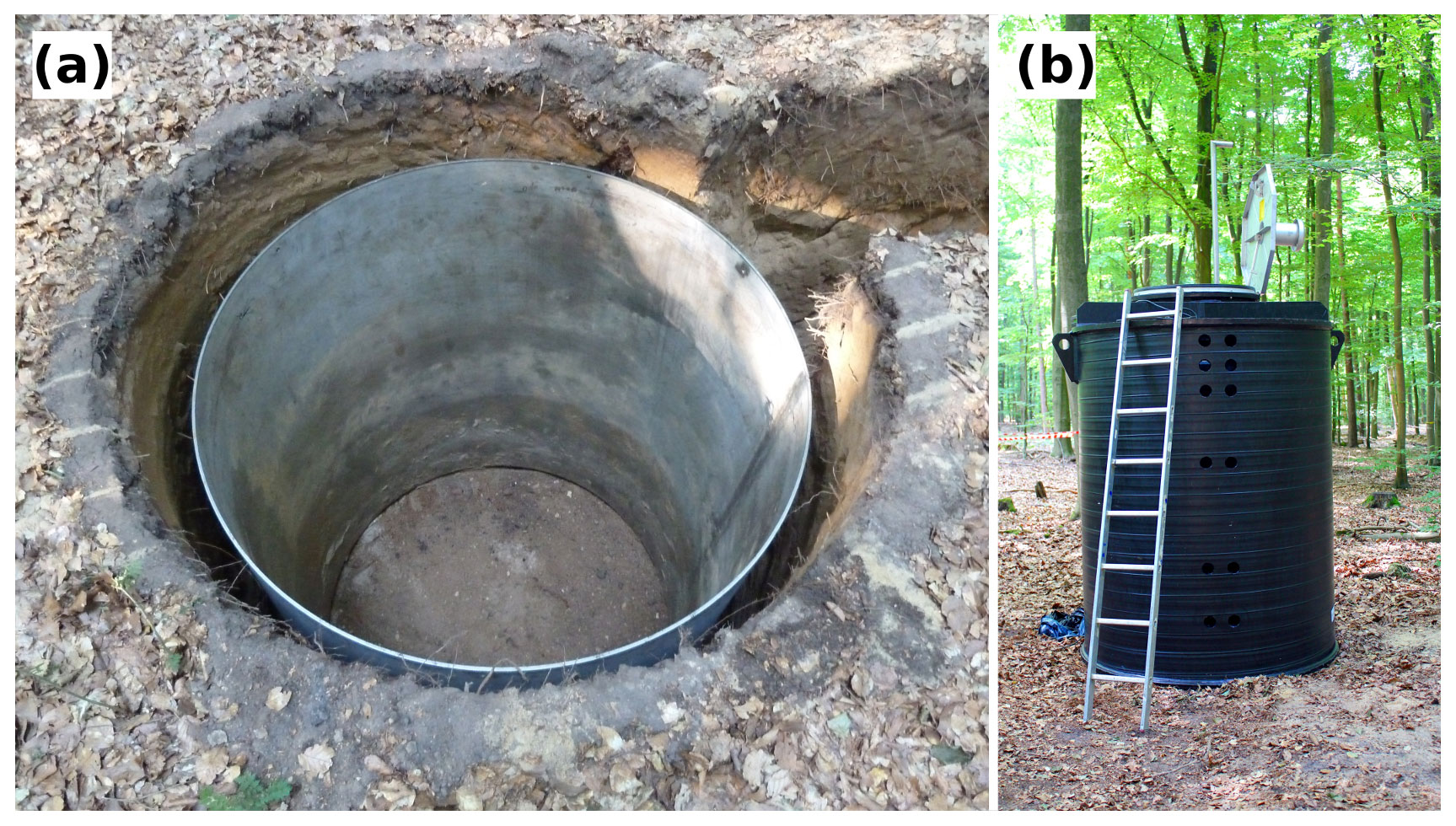
Figure 1Photographs of (a) the lysimeter vessels used to drill the hole for the subsoil observatories, and (b) the polyethylene shaft used as the subsoil observatory.
After the lysimeter vessel was removed, a polyethylene shaft (1.5 m in diameter and 2.1 m height) was placed in the soil (Fig. 1b) and is referred to here as the subsoil observatory. The gap (≈ 5 cm) between the subsoil observatory and the surrounding undisturbed soil was refilled. The observatories were installed close to one other, with a maximum distance of 30 m between them.
To monitor the temperature and volumetric water content, combined temperature and moisture sensors (UMP-1; Umwelt-Geräte-Technik GmbH, Germany) were installed at depths of 10, 30, 50, 90 and 150 cm, with a horizontal distance of 100 cm from the wall of the subsoil observatories (Fig. 2a). Measurements were taken every 15 min and stored on a data logger inside the subsoil observatory. The CO2 concentration in the soil air was monitored by solid-state infrared gas sensors (GMP221; Vaisala Oyj, Finland) with a measuring range of 0 %–10 % CO2. To protect the polytetrafluoroethylene (PTFE) membrane of the CO2 sensor from damage while being placed in the soil, the sensor was coated with an additional PTFE foil (616.13 P; FIBERFLON, Turkey) to allow gaseous diffusion and prevent water infiltration. The CO2 concentration was measured every 3 h to reduce power consumption. The CO2 sensors were turned on 15 min before the measurement itself, due to their warm-up time. In addition, PTFE suction cups (25 mm in diameter and 60 mm length) for soil air sampling with stainless steel tubing (2 mm inner diameter; ecoTech Umwelt-Meßsysteme GmbH, Germany) were installed adjacent to the CO2 sensors. The gas samplers and CO2 sensors were installed at the same depths as the temperature and moisture sensors. The horizontal distance of the gas samplers and CO2 sensors from the subsoil observatory wall increased from 40 to 100 cm with increasing soil depth (Fig. 2a).
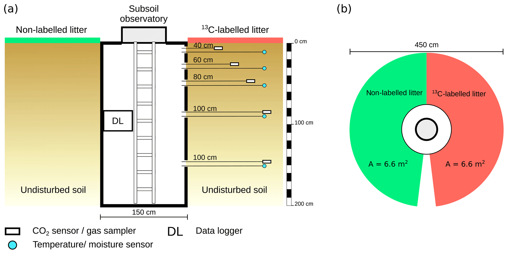
Figure 2Schematic overview of the subsoil observatories, the installed sensors and the labelling experiment. (a) Side view of the subsoil observatory. (b) Top view of the labelled and control area.
2.2 Gas sampling and measurements
2.2.1 Soil respiration
The surface CO2 efflux was measured using the closed-chamber method. A total of 30 PVC collars with a diameter of 10.4 cm and a height of 10 cm were installed 5 cm deep in the soil around the three subsoil observatories. The organic layer of 15 collars was removed in order to be able to distinguish between mineral soil respiration and total soil respiration. Soil respiration was measured with the EGM-3 SRC-1 soil respiration chamber (PP Systems, USA) and the LI-6400-09 soil chamber (LI-COR, Inc., USA). The measurement system was changed due to technical problems with the EGM-3 system; however, a comparison between the two systems revealed only minor differences. Each collar was measured three times per sampling day from March 2014 to March 2016, with sampling ranging from once a month to once a week. Annual soil respiration was derived from the linear interpolation of measured CO2 fluxes from the collars. Furthermore, soil respiration was modelled by fitting an Arrhenius-type model (Eq. 1), introduced by Lloyd and Taylor (1994) and using soil temperature data from 10 cm depth, and the measured CO2 fluxes as follows:
where F0 is soil respiration (µmol m−2 s−1), a, E0 and T0 are fitted model parameters, and T is the soil temperature at 10 cm depth (in degrees Celsius).
2.2.2 13CO2 sampling and measurement
In addition to continuous CO2 concentration monitoring, two gas samples per depth and subsoil observatory were taken at the end of the stainless steel tubing from the suction cups with a syringe and filled into 12 mL evacuated gas vials (Labco Exetainer; Labco Limited, UK). The sampling started in May 2014, with an interval of between once a month and once a week. The CO2 concentration in the soil gas samples was analysed by gas chromatography (Agilent 7890A; Agilent Technologies, Inc., USA). The δ13C values of the CO2 samples were measured by an isotope ratio mass spectrometer (Delta Plus with a GP interface and GC box; Thermo Fisher Scientific, Germany) connected to a PAL autosampler (CTC Analytics AG, Switzerland). The 13C results are expressed in parts per thousand (ppt) relative to the international standard of Vienna Pee Dee Belemnite (VPDB).
2.2.3 14CO2 sampling and measurement
Soil gas samples for radiocarbon analysis were taken in October and December 2014 in subsoil observatories 1 and 3. The CO2 was sampled using a self-made molecular sieve cartridge as described in Wotte et al. (2017). Briefly, each stainless steel cartridge was filled with 500 mg zeolite type 13X (40/60 mesh, charge 5634; IVA Analysetechnik GmbH & Co. KG, Germany), which is used as an adsorbent for CO2. The molecular sieve cartridges were connected to the installed gas samplers. The soil atmosphere of the corresponding depth was then pumped with an airflow of 7 mL min1 over a desiccant (Drierite; W. A. Hammond Drierite Co. Ltd, USA) to the molecular sieve cartridge for 40 min to trap the CO2 on the molecular sieve. Surface samples were taken from a respiration chamber (Gaudinski et al., 2000). The atmospheric CO2 inside the chamber was removed prior to sampling by circulating an airflow of ≈ 1.5 L min−1 from the chamber through a column filled with soda lime until the equivalent of 2–3 chamber volumes had been passed over the soda lime. Thereafter, the airflow was run over a desiccant and the molecular sieve cartridge for 10 min to collect the CO2 sample.
In the laboratory, the adsorbed CO2 was released from the molecular sieve cartridge by heating the molecular sieve under a vacuum (Wotte et al., 2017). The released CO2 was purified cryogenically and sealed in a glass tube. The radiocarbon (14C) analysis was directly performed on the CO2 with the gas ion source of the mini carbon dating system (MICADAS; Ionplus AG, Switzerland) at ETH Zurich (Ruff et al., 2010). The 14C concentrations are reported as fraction modern carbon (F14C), whereby F14C values of less than one denote that the majority of the C was fixed before the nuclear bomb tests in the 1960s, while values greater than one indicate C fixation after the bomb tests.
2.3 Labelling experiment
To trace the fate of fresh litter inputs in the soil and their contribution to the CO2 released from different soil horizons, a 13C labelling experiment was performed. In January 2015, the leaf litter layer around the subsoil observatories was removed and replaced with a homogeneous mixture of 237 g 13C-labelled and 1575 g non-labelled young beech litter, which is equal to a litter input of 250 g m−2. The labelled litter was distributed on a semi-circular area (6.6 m2) around the subsoil observatories (Fig. 2b). The labelled litter originated from young beech trees grown in a greenhouse in a 13CO2-enriched atmosphere. The mixture of labelled and non-labelled litter had an average δ13C value of 1241 ‰ for subsoil observatory 1 (OB1) and a δ13C value of 1880 ‰ for subsoil observatories 2 (OB2) and 3 (OB3).
2.4 Diffusivity measurements
Gas transport along the soil profile is determined by the diffusivity of the soil. The diffusivity of the soil was determined at depths of 10, 30, 50, 90 and 150 cm, with five undisturbed core sample replicates per depth and per observatory. To account for different water contents, the undisturbed soil cores (5.7 cm in diameter and 4.0 cm height) were adjusted in the laboratory at different matrix potentials (−30, −60 and −300 hPa) to cover a wide range of soil moisture. After the moisture adjustment, the soil cores were attached to a diffusion chamber as described in Böttcher et al. (2011). The diffusion chamber was flushed with N2 to initially establish a gas gradient between the chamber and the top of the sample as an atmospheric boundary condition. The increase in oxygen inside the ventilated chamber was measured over time with an oxygen dipping probe (DP-PSt3-L2.5-St10-YOP; PreSens Precision Sensing GmbH, Germany). Diffusivity and tortuosity factors (τ) were calculated with an inverse diffusion model (Schwen and Böttcher, 2013).
2.5 Data analysis
2.5.1 Gradient method
This method is based on the assumption that molecular diffusion is the main gas transport in the soil atmosphere. Therefore, gas fluxes, e.g. CO2 fluxes in a soil profile, can be calculated from the CO2 concentration gradient and the effective gas diffusion coefficient in the specific soil layer of interest.
In order to account for temperature and pressure dependencies of the CO2 sensors, the CO2 concentrations were corrected with a compensation algorithm for the GMP221 (S1) provided by the manufacturer (Niklas Piiroinen, Vaisala Oyj, Finland, personal communication, 2014). For the flux calculation, CO2 volume concentrations were converted to CO2 mole concentrations (Eq. 2) as follows:
where C is the CO2 mole concentration (µmol m−3), Cv is the CO2 volume fraction (µmol mol−1), p is the atmospheric pressure in Pascal (Pa), R is the universal gas constant (8.3144 J K−1 mol−1) and T is the soil temperature in kelvin (K) measured by temperature sensors at the corresponding soil depths. The CO2 flux of a soil layer was calculated using Fick's first law (Eq. 3) as follows:
where F is the diffusive CO2 flux (µmol m−2 s−1), Ds is the effective diffusivity in the soil atmosphere (m2 s−1) determined as described below, C is the CO2 concentration (µmol m−3) and z is the depth (metres). The equation is based on the assumption that (1) molecular diffusion is the dominating transport process in the soil atmosphere and other transport mechanisms – i.e. convective CO2 transport due to air pressure gradients or diffusion in the soil, and convective transport with soil water – are negligible, and (2) gas transport is 1D (e.g. De Jong and Schappert, 1972; Maier and Schack-Kirchner, 2014). The effective diffusivity Ds was calculated with Eq. (4) as follows:
where D0 is the CO2 diffusivity in free air. The pressure and temperature effect on D0 were taken into account by the following:
where Da0 is a reference value of D0 at standard conditions ( m2 s−1 at T0 293.15 K and p0 1.013×10⁵ Pa) (Jones, 1994). The dimensionless tortuosity factor τ at each depth was modelled as a function of the air-filled pore space ε for each soil depth. The model was derived from a power function fit from laboratory diffusion experiments (see above) on the undisturbed soil cores.
To account for the non-uniform vertical distribution of the soil water content in the soil profile, Ds was estimated as the harmonic average between the two measurement depths (Pingintha et al., 2010; Turcu et al., 2005) as follows:
where Δz1,2 (metres) is the thickness of the corresponding soil layer, and is the effective diffusivity of the respective soil layer. Finally, assuming a constant flux between measured CO2 at depth zi and zi+1, the CO2 flux (Fi) was calculated by combining Eqs. (2)–(6) as follows:
where Fi is the CO2 flux (µmol m−2 s−1) at the upper boundary (zi) between depth zi and zi+1 (metres). To calculate soil respiration (F0) at the surface with the gradient method, a CO2 concentration of 400 µmol mol−1 at the soil surface and a constant Ds for the first 10 cm were assumed.
2.5.2 CO2 production
The CO2 production (Pi) in a soil layer was calculated as the difference between the flux (Fi) leaving the specific soil layer at the upper boundary (zi) and the input flux (Fi+1) at the lower boundary (zi+1) of the specific soil layer. Therefore, Pi had the unit of a flux (µmol m−2 s−1) (a similar approach was done by, for example, Gaudinski et al., 2000; Hashimoto et al., 2007; Fierer et al., 2005; Davidson et al., 2006).
Total soil respiration was calculated as the sum of CO2 production in all soil layers. Equation (8) is based on the assumption of a steady-state diffusion. Steady-state conditions for CO2 concentration and volumetric water content were mostly given, except during a few heavy rain events where steady-state conditions were not met due to changing water contents in the profiles. Most soils exhibit increasing CO2 concentrations with increasing soil depth. Therefore, CO2 production is mostly positive with upward CO2 fluxes. However, if the CO2 concentration in a soil layer is greater than in the layers below, the calculated CO2 production in the layers below can become negative (downward directed). Hence, in the present study, no CO2 production was assumed when the calculated CO2 production in a soil layer was negative. This approach was based on the assumption that there are no relevant CO2 sinks in the soil profile. Furthermore, negative CO2 production is considered as CO2 storage, which will be released if the CO2 concentration gradient or diffusion conditions change. In OB1, negative CO2 production values were calculated in the first year at 30–50 cm depth (331 out of 365 d) and at 50–90 cm depth (359 out of 365 d). In the second year, negative values also occurred in OB1 at 30–50 cm depth (8 out of 308 d) and at 50–90 cm depth (182 out of 308 d).
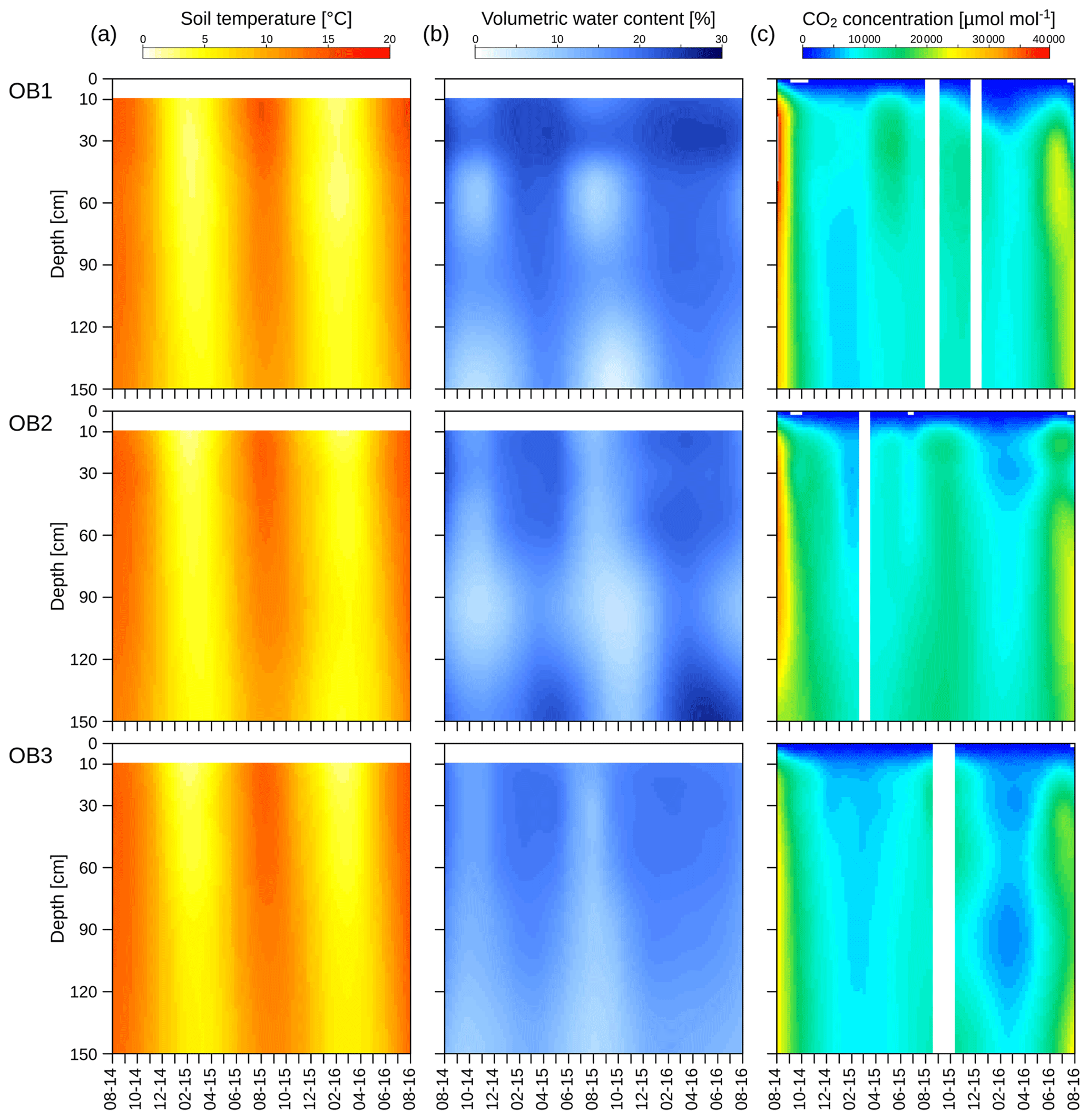
Figure 3Soil profile measurements of temperature (a), volumetric water content (b) and CO2 concentration for the three observatories (OB). White bars represent periods without measurements.
2.5.3 Isotopic composition of CO2
To determine the contribution of the labelled leaf litter to CO2 in the soil atmosphere, we used the isotopic mixing equation (Eq. 9) as follows:
where δ13CM is the isotopic signature of the gas sample, δ13CL is the isotopic signature of the labelled leaf litter (1241 ‰ for OB1 and 1880 ‰ for OB2 and OB3), and δ13CB is the average isotopic signature of the soil atmosphere for each observatory and depth before the labelled leaf litter was applied, assuming there was no change.
The CO2 fluxes and productions for each layer and isotopologue of CO2 (12CO2 and 13CO2) were calculated using the isotopic signature of the soil atmosphere and Eqs. (2)–(7). To account for different effective diffusivities of 12CO2 and 13CO2, the effective diffusivity Ds for 13CO2 was adjusted, according to Cerling et al. (1991), as follows:
where it is assumed that Ds is equivalent to 12Ds due to the fact that about 99 % of total CO2 is 12CO2.
To determine the contribution of the labelled leaf litter to the CO2 production in a soil layer and accounting for diffusion effects, the isotopic signature of CO2 production (δ13P-CO2) in each soil layer was calculated with Eq. (11) as follows:
where Rst is the isotopic ratio of the VPDB reference standard, while 13P-CO2 and 12P-CO2 are the CO2 production for each isotopologue of the respective soil layer. Afterwards, Eq. (9) was used to calculate the amount of labelled leaf litter to total CO2 production, where δ13CB was substituted with the average isotopic signature of CO2 production (Eq. 11) before the labelling, and δ13CM was substituted with the isotopic signature of CO2 production. The litter-derived CO2 production was calculated by multiplying the amount of labelled leaf litter (L) with the total CO2 production of the respective soil layer.
2.6 Statistical analysis
A Monte Carlo simulation was generated to determine the influence of the measurement uncertainties of the sensors, which were used for calculation of CO2 fluxes and CO2 production rates. It was assumed that each measurement error was normally distributed. The standard deviation was equal to the measurement accuracy, which was obtained from the corresponding manual. The distributions of CO2, volumetric water content and temperature measurements were used for 1000 Monte Carlo simulations. Unless stated otherwise, the error bars in the final results represent the standard deviation of these simulations. All analyses were performed in R (version 3.3.2) for Linux (R Core Team, 2017).
3.1 Temperature, water content and CO2 concentration in the profile
Soil temperature showed a distinct seasonality down to 150 cm, with the maximum and the minimum temperatures delayed with increasing soil depth (Fig. 3a). The minimum soil temperature was 0.3 and 4.0 ∘C in January 2016 at 10 and 150 cm depths respectively. The maximum temperature was measured in July in the uppermost layer (16.6 ∘C) and in August in the deepest layer (14.4 ∘C). The annual amplitude of the soil temperature decreased from 16.3 ∘C at 10 cm to 10.4 ∘C at 150 cm. However, mean annual values showed no significant decline with soil depth and were 8.4 and 8.3 ∘C at 10 and 150 cm respectively during the 2 years of observation. Variations in the mean soil temperatures between the three observatories were <1 ∘C at all depths (Fig. S1).
The volumetric water contents also showed seasonal variations at all depths (Fig. 3b), with depletion during the summer. The minimum of the volumetric water content at 10 cm was reached in August (10 %), whereas the minimum at 150 cm was observed 2 months later in October (6 %). The water reservoir of the soil profile was refilled during the autumn and winter, reaching maximum values at 10 cm (23 %) and 150 cm (22 %) in April (Fig. 3b), which were delayed by 14 d in the deepest layer. In OB1 and OB3, the mean volumetric water content decreased with increasing soil depth. Only in OB2 did the mean water content increase at 150 cm (Fig. S2). The water content showed a greater variation between the three observatories than in the soil temperature (Fig. S2).
The CO2 concentration in the soil pores followed a similar seasonality to the soil temperature (Fig. 3c), with a maximum during the summer and a minimum during the winter and early spring. The same behaviour was observed for both investigated years, while the values were higher during the first summer. The CO2 concentration in the uppermost layer ranged from 1000 to 35 000 µmol mol−1 and, thus, was in a similar range of results for the deepest layer, with 7500 to 35 000 µmol mol−1. However, values were highly variable between the observatories, with OB2 and OB3 showing an increasing CO2 concentration with greater soil depth, whereas OB1 yielded the highest CO2 concentrations at 30 to 50 cm depth.
3.2 Soil respiration
The mean annual mineral (without the organic layer) soil respiration determined with chamber measurements for the three observatories was 776±193 g C m−2 yr−1, with a small variability between the observatories (Table 1). The mineral soil respiration modelled with the Lloyd–Taylor function gave similar results for the same period. In contrast, soil respiration determined with the gradient method showed a high variability between the observatories, but was in the range of the directly measured respiration, except for OB1. This variability can be explained by the higher water content at OB1 and, consequently, the lower diffusion coefficient. The average diffusion coefficient at OB1 at 10 cm was less than half that at OB2 and OB3.
Table 1Total soil respiration with and without the organic layer for the three observatories derived from soil surface measurements with linear interpolation (chamber), modelled with a Lloyd–Taylor function and derived from the gradient method based on CO2 measurements along the soil profile for 1 year. Means and standard deviations are shown.
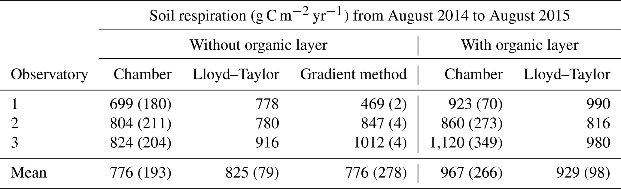
The organic layer increased total respiration by 13 % and 25 % respectively for the Lloyd–Taylor model and chamber measurements (Table 1). For all the methods and in all the observatories, soil respiration correlated well with soil temperature and soil moisture. The highest fluxes were measured when soil temperature (10 cm) was highest and water content (10 cm) was low (Figs. 3 and 4).
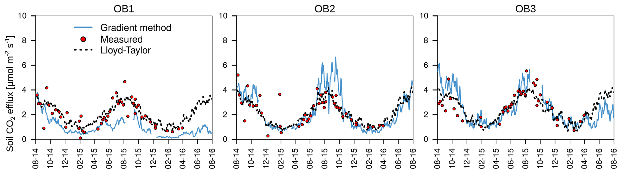
Figure 4Mean daily soil respiration determined with the gradient method, measured with chambers and modelled with a Lloyd–Taylor function for the observatories (OB).
3.3 Vertical CO2 production
The mean CO2 production rates decreased from 1.4 µmol m−2 s−1 in the uppermost layer (0–10 cm depth) to 0.03 µmol m−2 s−1 in the deepest layer (50–90 cm depth; Fig. 5). The CO2 production followed the same seasonality as soil temperature and CO2 concentration, with the highest production rates occurring during the summer and the lowest during the winter months in all soil layers. This seasonal variation was greatest in the top two layers of the soil (0–10 and 10–30 cm; Fig. 5a–d).
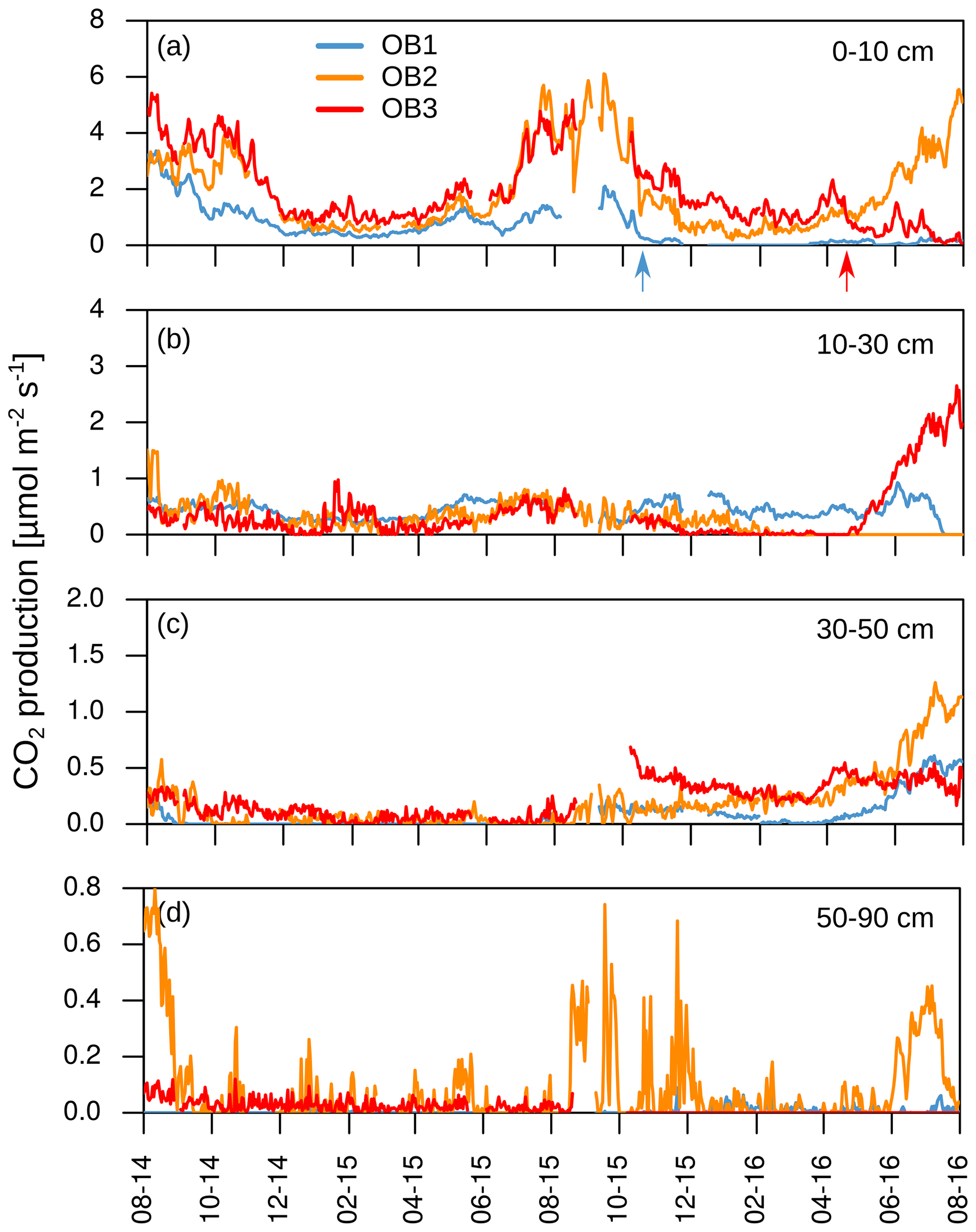
Figure 5(a–d) Daily mean CO2 production in each soil layer. Arrows indicate disturbances due to bioturbation of voles close to the CO2 sensors at 10 cm depth (OB1 and OB3), which created macropores and changed diffusivity.
About 70±17 % of total soil respiration was produced in the first 10 cm of the soil profile where 21 % of the SOC stock (0–1.5 m) was stored. The CO2 production at 10 to 30 cm accounted for 20 ± 14 % of the total soil respiration during the year, and 32 % of the SOC was located in this depth increment. The subsoil (>30 cm) accounted for 10 ± 9 % of total CO2 production, with 47 % of the SOC stock stored in the subsoil.
The mean total CO2 production showed no significant differences between the 2 years. The variation in total annual CO2 production was greater between the three observatories (326–1008 g CO2-C m−2 yr−1) than between the 2 studied years (Fig. 6). However, the CO2 production in the different soil layers showed considerable changes with time; it increased by 500 % in the subsoil, from 30 to 50 cm, in the second year, which increased the contribution of subsoil CO2 production from 4 % to 16 % of the total CO2 production. This increase was observed at all three observatories. In contrast, the CO2 production in the first 10 cm in OB1 and OB3 showed a decline from the first to the second year, which was probably caused by methodological variations and does not represent a real decrease in respiration activity since the bioturbation of animals (e.g. voles) might have had a strong influence on the diffusivity (Fig. 5a). Voles created macropores; therefore, the CO2 gradient approach was not applicable. This was also indicated by a sudden and rapid drop in CO2 production between 0 and 10 cm in OB1 (October 2015) (Fig. 5a).
To take the different SOC contents of each soil layer into account, the cumulative CO2 production was normalised to the SOC stock of the respective layer (Fig. 7). The specific CO2 production decreased from 322 g CO2-C kg−1 SOC yr−1 in the first 10 cm to 9 g CO2-C kg−1 SOC yr−1 at 50 to 90 cm. It should be noted that the proportion of autotrophic respiration in the total CO2 production could not be quantified.
3.4 Sources of CO2 production
3.4.1 Contribution of fresh litter
The isotopic signature of soil CO2 (δ13CO2) in the observatories before the start of the labelling experiment ranged from −25.4 ‰ to −21.8 ‰, with no significant differences between soil depths (Fig. 8a). The labelling experiment was conducted to assess the fate of fresh litter added on top of the organic layer into different C fractions (e.g. SOC and DOC), including soil CO2. A total of 6 d after the application of the 13C-labelled leaf litter, CO2 was already enriched in litter-derived C down to 90 cm depth in all the observatories. The isotopic signature ranged from 70 ‰ at 10 cm depth to −19 ‰ at 90 cm depth (Fig. 8b). Thus, the maximum contribution of litter-derived C to total CO2 was 5 % at 10 cm depth 6 d after the litter replacement (Fig. 8c). At 90 cm, the maximum amount of litter-derived CO2 was 0.6 % 2 weeks after the beginning of the labelling experiment (Fig. 8c). In addition, minor peaks with up to 0.8 % of CO2 derived from the labelled litter were observed at all depths after rain events within the first 6 months of litter application. The average contribution of litter-derived CO2 decreased with time and reached a range of 2.5 % to 0.2 % at 10 cm depth from January 2015 to July 2016. The total amount of labelled litter-derived C to the CO2 production below 10 cm was 291 mg C m−2 (±127) (Fig. 9), which accounted for 0.12 % of the total CO2 production below 10 cm depth.
Assuming that diffusion is the main transport process of CO2 in the soil atmosphere, the CO2 flux between two soil layers can be calculated for each C isotope separately. As mentioned, a positive flux indicates the release of CO2 from mineralisation or root respiration in the respective soil layer. A negative flux, in turn, represents the downward diffusion of CO2 from the layer above. Due to the high 13C enrichment in the applied litter, negative 13CO2 fluxes can indicate a downward diffusion of litter-derived CO2 from the soil layer above (Fig. 10). On average for the three observatories, 20 out of 41 samplings had negative 13CO2 fluxes below 90 cm depth, indicating a downward movement of labelled litter-derived CO2. Furthermore, OB2 and OB3 had positive 13CO2 fluxes between 10 and 90 cm, indicating a transport of labelled litter-derived C down the soil profile as dissolved organic carbon (DOC) and mineralisation of this DOC. Meanwhile, the observed 13C enrichment in CO2 in OB1 below 30 cm depth might also be influenced by diffusion of labelled litter-derived 13CO2 from the soil layer above (10 to 30 cm).
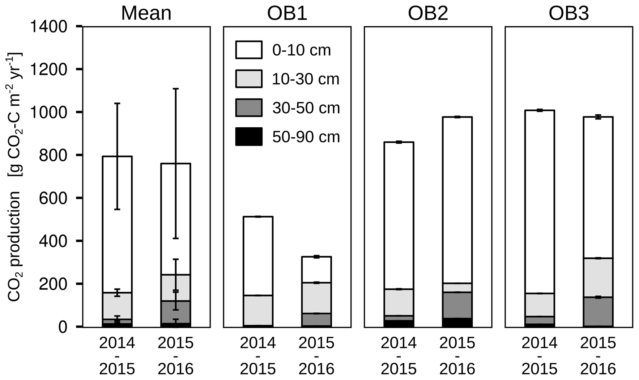
Figure 6Cumulative CO2 production for each soil layer, observatory (OB) and year of observation. Error bars represent the standard deviation.
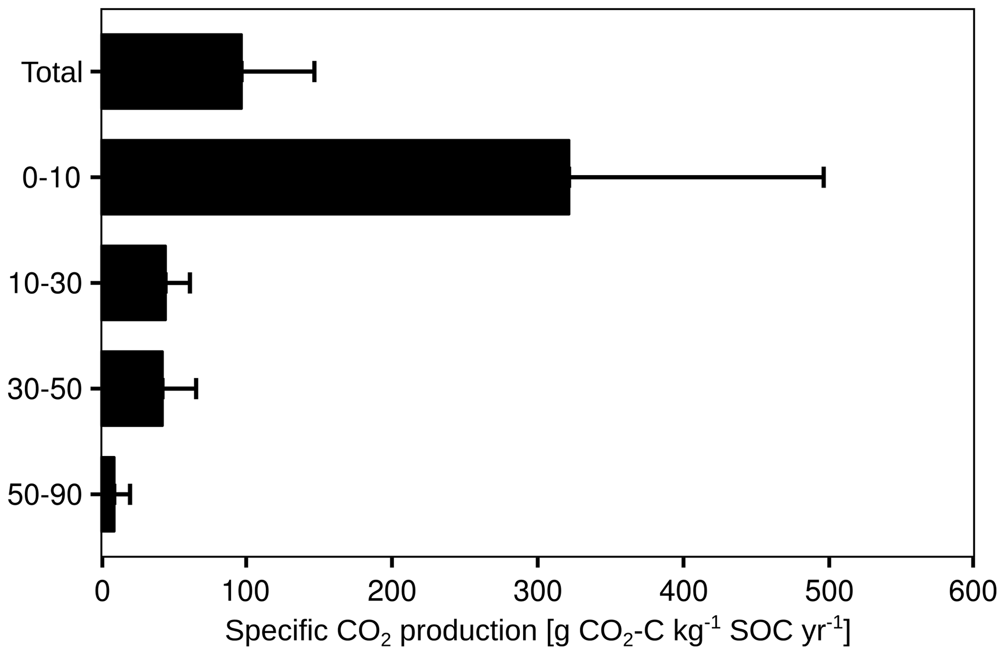
Figure 7Annual specific CO2 production for the total CO2 efflux. Mean (n=3) and standard deviation are shown.
3.4.2 Contribution of old C
The radiocarbon content of the bulk SOC decreased strongly with increasing soil depth from close to atmospheric values (F14C 0.99) at 10 cm to an apparent age of about 3460 years before the present (F14C 0.65) at 110 cm depth (Fig. 11; grey triangles). In contrast, the 14C concentrations of the CO2 in the soil atmosphere were relatively constant throughout the soil profile and for both samplings, with values in the range of 1.03–1.07 F14C and, thus, they derive mainly from the post-bomb period (Fig. 11; black dots). This indicates a young source of CO2 production. Consequently, old subsoil SOC was not detected as a significant source of CO2 production.
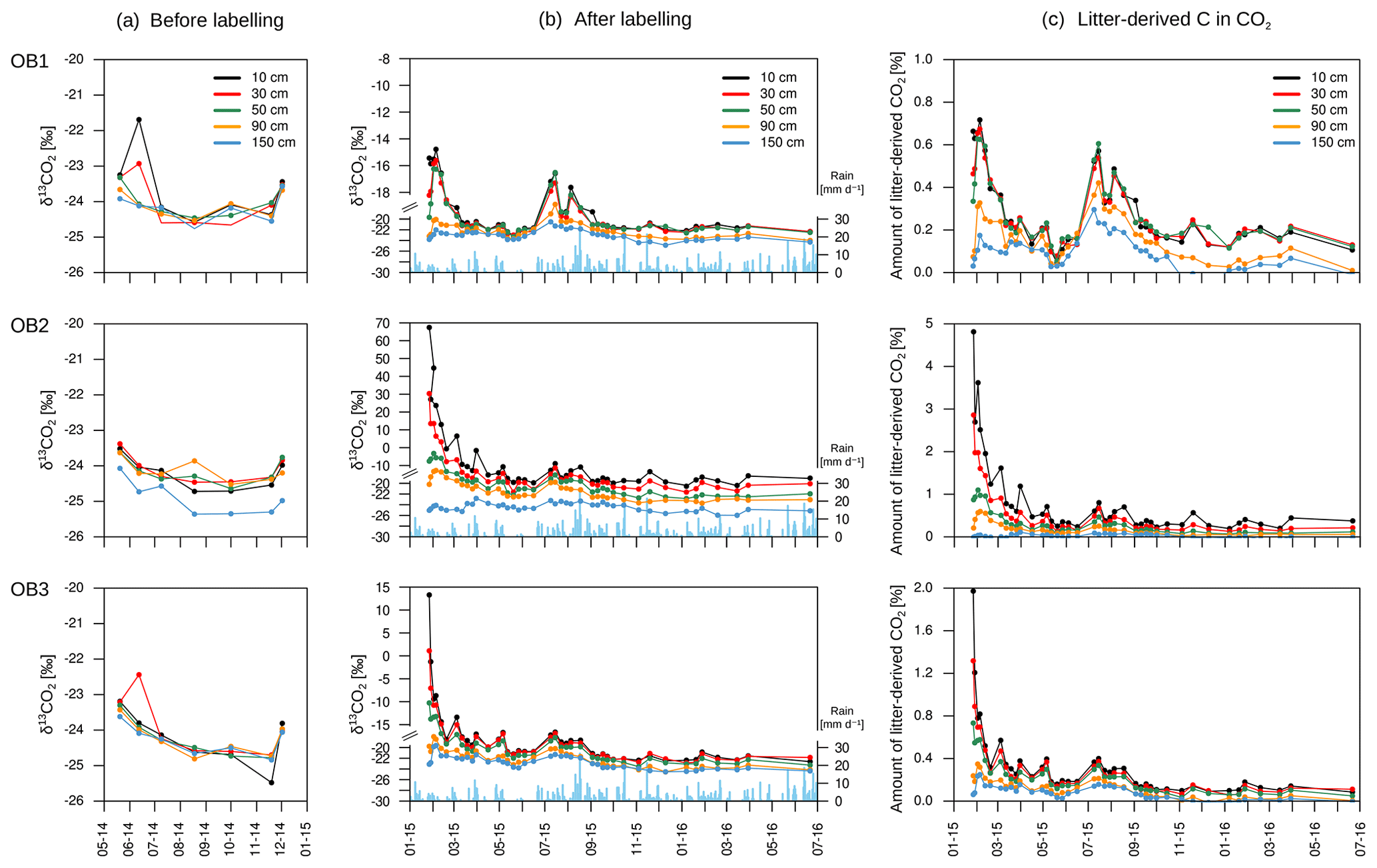
Figure 8Isotopic signature of CO2 at each depth and observatory (OB) before the addition of the labelled litter (a) and after the labelled litter addition (b), with daily precipitation data (blue bars). The relative amount of litter-derived CO2 on total CO2 at each depth and observatory (c). Please note the different y-axis ranges for (b) and (c).
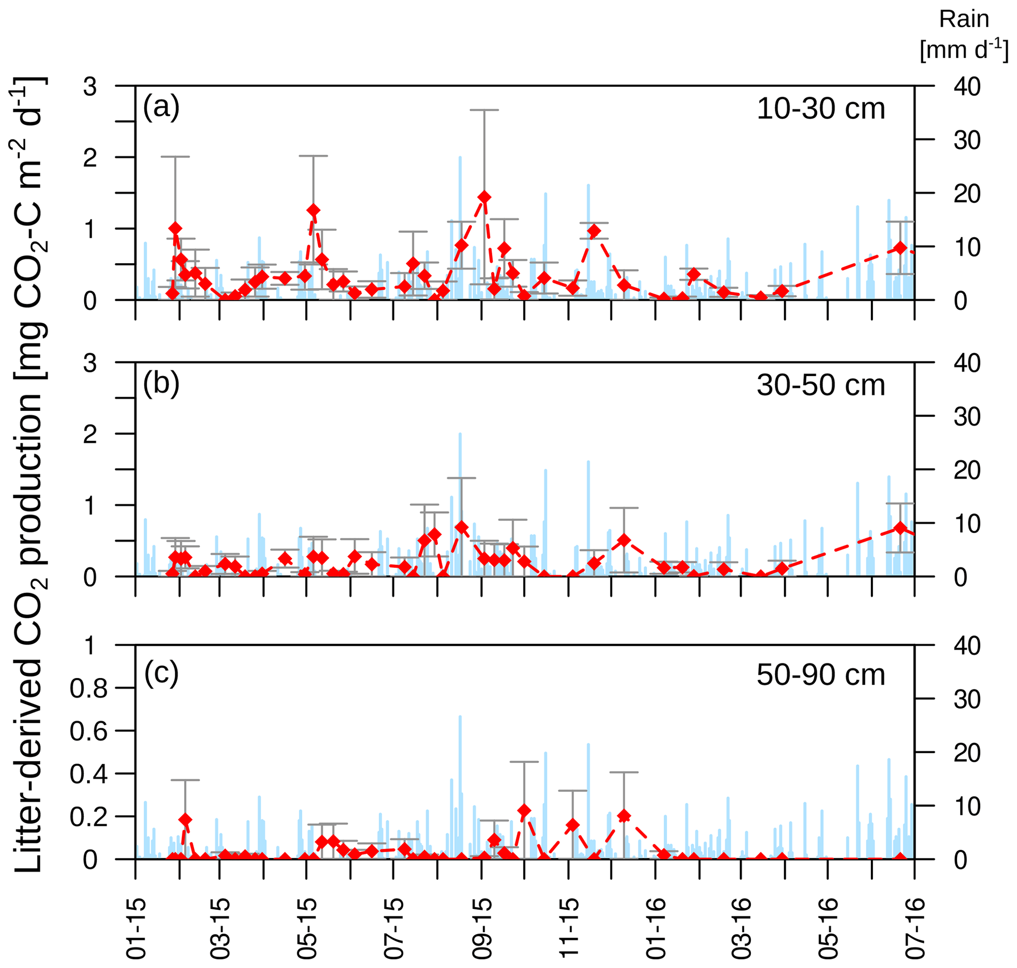
Figure 9(a–c) Litter-derived CO2 production in each soil layer. Mean (n=3) and standard error are shown.
4.1 Temperature, water content and CO2 concentration in the profile
In all three subsoil observatories, increasing CO2 concentrations with depth were observed. This has also been reported by other studies (Davidson et al., 2006; Drewitt et al., 2005; Fierer et al., 2005; Hashimoto et al., 2007; Moyes and Bowling, 2012). However, the increase was not continuous down to 150 cm depth. Higher CO2 concentrations were observed between 30 and 50 cm depth, indicating a higher CO2 production at this depth increment, which can be linked to the root distribution in the subsoil observatories (Fig. 12). About 82 % of the fine root biomass and necromass were found to be located between 0 and 50 cm and 18 % at the 30 to 50 cm depth. Therefore, the contribution of autotrophic respiration to CO2 production and the mineralisation of dead roots were greater at these depths than in the deep subsoil (>50 cm). The CO2 concentration in the soil pores is also controlled by abiotic factors such as effective diffusivity (Ds). The average effective diffusivity (Ds) at 10 cm was about 40 % lower than at 30 cm. Consequently, CO2 accumulated in the soil pores below 10 cm depth due to the lower diffusion of CO2 between the soil surface and 10 cm depth. The effective diffusivity was mainly controlled by soil water content, which reduced it. For example, the high CO2 concentration in August 2014 (up to 40 000 µmol mol−1) compared to August 2015 (up to 20 000 µmol mol−1; Fig. 3c) can be explained by the higher volumetric water content in 2014 in all profiles. The high water content was related to more precipitation in July 2014 (120 mm) than in July 2015 (47 mm) and to less precipitation in August in both years (49 and 95 mm). Additionally, evapotranspiration was greater in August 2015 than in August 2014 due to a higher mean air temperature (18 and 15 ∘C).
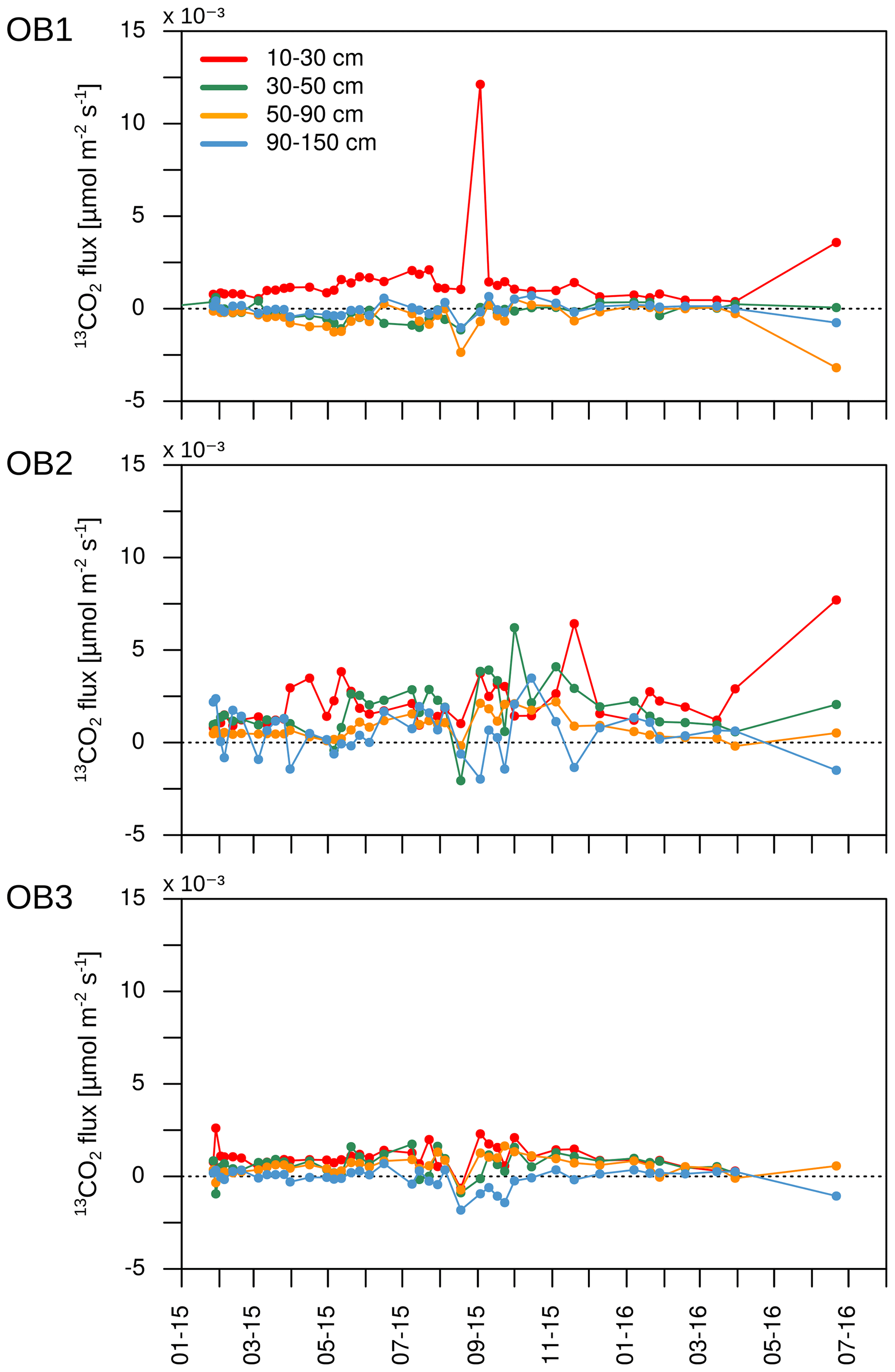
Figure 1013CO2 fluxes for each observatory. Negative fluxes represent the diffusion of 13CO2 from the soil layer above.
4.2 Soil respiration
The annual mean total respiration determined using the gradient method corresponded well with the results of the closed chamber measurements, indicating that the gradient method resulted in realistic flux estimations (Table 1; Fig. 4). This is in line with the results reported by other studies (Baldocchi et al., 2006; Tang et al., 2003; Liang et al., 2004). The differences in soil respiration between the methods can be attributed to the different spatial resolutions of the corresponding measurements. The chamber measurements were based on five spatial replicates for each subsoil observatory, covering a total measurement area of 1274 cm2. Therefore, chamber measurements accounted for spatial variability in water content and soil CO2 concentrations below the chamber, whereas the gradient method was based on one profile measurement for CO2 and water content at each of the three observatories. Large differences in total respiration rates of up to 200 % were found among the three observatories with the gradient method. Both methods have advantages and disadvantages for determining total soil respiration. The gradient method does not alter the soil atmosphere CO2 gradient, and is continuous and less time-consuming than chamber measurements, but it is vulnerable to the spatial heterogeneity of the soil structure, moisture content around the sensors and changes in diffusivity, e.g. due to bioturbation. For example, the higher soil respiration determined with the gradient method at OB2 and OB3 in summer (Fig. 4) is linked to lower soil moisture measured in 10 cm depth (Fig. 3b) and to higher total soil porosity (51 % at OB2 and 49 % at OB3 vs. 46 % at OB1). As a consequence, the effective diffusivity (Eq. 4) is higher, resulting in higher fluxes. Furthermore, the lower soil respiration of OB1 and OB3 in the second year, determined with the gradient method, was related to the bioturbation of voles, which increased the diffusivity around the CO2 sensors and led to a lower CO2 concentration in 10 cm depth, which in turn led to an underestimation of the total soil respiration (Fig. 4) by the gradient method.
Removing the organic layer in the soil collars was supposed to determine the contribution of CO2 production in the organic layer to total soil respiration. Since the organic layer was only removed in the soil collars and not around the soil collars, it must be noted that the contribution of the organic layer to total soil respiration might be underestimated with the used method. However, the results are in line with findings from litter manipulation experiments, which reported a contribution of 9 % to 37 % of the organic layer to total soil respiration (Nadelhoffer et al., 2004; Bowden et al., 1993; Kim et al., 2005; Sulzman et al., 2005).

Figure 11Mean 14C concentration (F14C) of bulk soil (grey triangles; data from Angst et al., 2016) and CO2 in the soil atmosphere (black dots). The solid black lines represent the annual average F14C values in the atmosphere from 2014, measured at the Jungfraujoch alpine research station, Switzerland (Ingeborg Levin and Samuel Hammer, personal communication, 2015).

Figure 12Mean fine root density for biomass and necromass of the subsoil observatories. Error bars represent the standard error.
4.3 Vertical CO2 production
The vertically partitioned CO2 flux revealed that more than 90 % of the total CO2 efflux was produced in the topsoil (<30 cm). These results correspond well with other studies which have found that more than 70 % of total CO2 efflux in temperate forests is produced in the upper 30 cm of the soil profile (Davidson et al., 2006; Fierer et al., 2005; Hashimoto et al., 2007; Jassal et al., 2005; Moyes and Bowling, 2012). Nevertheless, only 53 % of the SOC stock is stored in the first 30 cm, indicating that subsoil SOC on the site of the present study may have a slower turnover than the topsoil SOC. This is supported by the low 14C concentrations in SOC below 30 cm. However, the higher CO2 production in the topsoil can be also related to a greater fine root biomass and necromass density (Fig. 12), which may serve as an indicator of autotrophic respiration and heterotrophic respiration in the rhizosphere. Even if the current study is unable to distinguish between autotrophic and heterotrophic respiration, the importance of autotrophic respiration to total soil respiration was shown in a large-scale girdling experiment by Högberg et al. (2001). They reported that autotrophic respiration accounted for up to 54 % of total soil respiration. As a consequence, autotrophic respiration should be higher in the topsoil than in the subsoil, due to the decreasing root bio- and necromass with increasing soil depth (Fig. 12).
It is remarkable that the CO2 production at 30 to 50 cm increased from 23 g C m−2 yr−1 in the first year to 118 g C m−2 yr−1 in the second year of the study (Fig. 6). This can be explained in part by more precipitation in the second year (621 mm) than in the first year (409 mm), inducing fewer water-limiting conditions for plants and microbial activity. As a result, the mean volumetric water content was higher in the second year (18 % compared to 16 %) at 50 cm depth, which gave better conditions for the mineralisation of SOC by microorganisms (Cook et al., 1985; Moyano et al., 2012). Furthermore, the greater precipitation increased the input of DOC into the subsoil on the site of the present study, which is supported by the study of Leinemann et al. (2016), who investigated DOC fluxes in subsoil observatories for more than 60 weeks. They found a positive correlation between DOC fluxes, precipitation and water fluxes at 10, 50 and 150 cm depths. Furthermore, they showed that DOC fluxes declined by 92 % between a depth of 10 and 50 cm, which was attributed to mineral adsorption and microbial respiration of DOC (Leinemann et al., 2016).
4.4 Sources of CO2 production
4.4.1 Young litter-derived CO2
In this study, a unique labelling approach was used to estimate the contribution of aboveground litter to CO2 production along a soil profile by applying stable isotope-enriched leaf litter to the soil surface. These results showed that litter-derived C did not significantly contribute to annual CO2 production below 10 cm depth. Leaf litter is decomposed and washed into the mineral soil as DOC. Within 1 year, only 0.13 % of total CO2 production between 10 and 90 cm originated from the labelled leaf litter. It should be considered that part of the measured 13CO2 may derives from the turnover of the microbial necromass, which could lead to an overestimation of the litter-derived CO2. However, the isotopic signature of the biomass at the study site ranges from −27 ‰ (10 cm) to −25.8 ‰ (90 cm; Sebastian Preußer and Ellen Kandeler, personal communication, 2020) which is lower than the isotopic signature of the soil atmosphere before the application of the labelled leaf litter. This indicates that the turnover of microbial biomass had no measurable effect on the isotopic signature of the soil atmosphere. Instead, it should be mentioned again that the determination of the CO2 production is based on the assumption of steady-state conditions in the soil. Sudden changes in the CO2 concentration or soil moisture, for example, after precipitation events can lead to a violation of this assumption, and the uncertainties in litter-derived CO2 production increase for these periods. A non-steady-state model might be better to describe such periods, but a non-steady-state model may also require a higher spatial and temporal resolution of measurements (water content, CO2 and 13CO2) at depths of 0–10 cm. Nevertheless, further research should address this point. However, in periods without major precipitation events (before the 13CO2 sampling) the contribution of litter-derived CO2 to total CO2 remained below 1 %. This indicates that, despite the uncertainties due to non-steady-state conditions, the mineralisation of DOC originating from the organic layer was a minor source of CO2 production in the soil profile below 10 cm. The average DOC flux in the subsoil observatories in the first year was estimated to be 20 g C m−2 yr−1 at 10 cm depth and 2 g C m−2 yr−1 at 50 cm depth, indicating a DOC input of 18 g C m−2 yr−1 into the 10 and 50 cm depth increments (Leinemann et al., 2016). An assumed complete mineralisation of this DOC would account for 11 % of CO2 production at this depth increment. Overall, most of the CO2 production between a depth of 10 and 90 cm must be derived from autotrophic respiration and heterotrophic respiration in the rhizosphere.
4.4.2 Old SOC derived CO2
The very similar radiocarbon contents of soil CO2 produced at different depths, which were 1.06 F14C on average, revealed that ancient SOC components were not a major source of CO2 production. The results indicate that the CO2 originated mainly from young (several decades old) C sources, presumably mainly from root respiration, its exudates and DOC. Other studies have found similar results at a grassland site in California down to 230 cm depth (Fierer et al., 2005) and in temperate forests down to 100 cm (Gaudinski et al., 2000; Hicks Pries et al., 2017). In addition, Hicks Pries et al. (2017) incubated root-free soil from three depths (15, 50 and 90 cm) and compared the radiocarbon signature of the respired CO2 with their results from the field. They found that CO2 from the short-term incubations had the same modern signature as the field measurements despite the high 14C age of the bulk SOC at 90 cm depth (∼1000 yr BP; Hicks Pries et al., 2017). This supports the findings of the present experiment. Therefore, microbial respiration in temperate subsoils is mainly fed by relatively young C sources fixed less than 60 years ago.
4.4.3 Diffusion effects
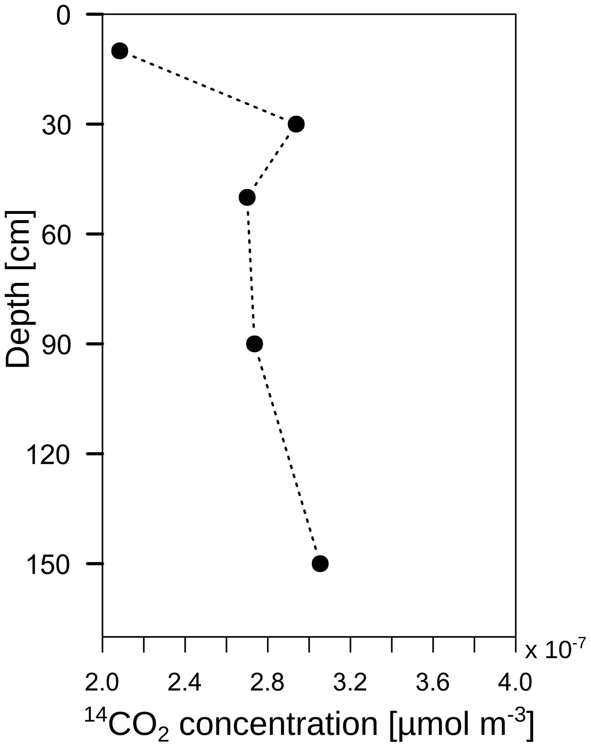
A highly 13C-enriched CO2 source was introduced to the top of a soil profile. Shortly afterwards, an enrichment of 13C was measured in CO2 along the whole soil profile (Fig. 8b). However, this enrichment could not only be linked to the transport and mineralisation of litter-derived C along the soil profile (e.g. DOC in seepage water). The diffusion of 13CO2 down the soil profile also has to be taken into account. According to Fick's first law, 13CO2 diffuses into the soil profile following the 13CO2 gradient independently from the 12CO2. Thus, even though the total CO2 concentration increased with soil depth, meaning an upward diffusion of 12CO2, the 13CO2 gradient could be the opposite due to 13C-enriched leaf litter, leading to a downward diffusion of 13CO2. Consequently, this could lead to a misinterpretation of the pathways of subsoil 13CO2 in tracer experiments. Furthermore, this effect should also be taken into consideration when interpreting 14CO2 soil profile measurements as an indicator of the age of the mineralised SOC, as in other field studies (e.g. Davidson et al., 2006; Davidson and Trumbore, 1995; Fierer et al., 2005; Gaudinski et al., 2000). Downward diffusion of 14CO2 might be an important factor for explaining the observed 14CO2 profiles. If this downward diffusion is the case, the 14CO2 gradient should not have a continuous decrease with soil depth since the 14CO2 gradient is the driving factor for diffusion according to Eq. (3). In fact, 14CO2 concentration at 30 cm depth in subsoil OB1 was greater than at 50 cm depth (Fig. 13), which in turn led to a downward diffusion of 14CO2 from a depth of 30 to 50 cm. This might lead to a rejuvenation in the 14CO2 soil profile and to an underestimation of the mineralisation of old SOC in subsoils.
The gradient method allowed total soil respiration to be partitioned vertically along a soil profile. Most of the CO2 (90 %) was produced in the topsoil (<30 cm). However, the subsoil (>30 cm), which contained 47 % of the SOC stocks, accounted for 10 % of total soil respiration. This can be explained by a larger amount of stable SOC in subsoils compared to topsoils. However, the modern radiocarbon signature of CO2 throughout the soil profiles indicated that mainly young carbon sources were being respired from roots and root exudates and autotrophic respiration. The contribution of old SOC to subsoil CO2 production was too small to significantly alter the 14C concentrations in the soil atmosphere used to identify CO2 sources. Furthermore, this study showed that the mineralisation of fresh litter-derived C only contributed to a small part of total soil respiration, underlining the importance of roots and the rhizosphere for subsoil CO2 production.
All raw data (without 14C) can be accessed in a data package via https://doi.org/10.25532/OPARA-101 (Wordell-Dietrich, 2020).
The supplement related to this article is available online at: https://doi.org/10.5194/bg-17-6341-2020-supplement.
All the authors contributed to the design of the field measurements, and PWD carried out the field measurements. The preparation of the 14CO2 samples was performed by PWD and AW. Data analysis and modelling were performed by PWD. KK took the root samples, analysed them and provided the data. PWD took the lead in writing the paper, with contributions from all the co-authors.
The authors declare that they have no conflict of interest.
We acknowledge support from the open access publication funds of the SLUB/TU Dresden for financing this open access publication. We would like to thank Jens Dyckmanns and Reinhard Langel from the Centre for Stable Isotope Research and Analysis at the University of Gö̈ttingen for the 13CO2 measurements. We also want to thank Frank Hegewald and Martin Volkmann for their support in the field, especially with changing the heavy (23 kg) batteries in the subsoil observatories every month. We would also like to thank Ullrich Dettmann for his support with R, and many thanks go to Heiner Flessa, Marco Gronwald, Cora Vos and Viridiana Alcantara for the fruitful discussions and recommendations. Finally, we thank the reviewers for their comments.
This research has been supported by the Deutsche Forschungsgemeinschaft (grant no. HE 6877/1-1).
This paper was edited by Luo Yu and reviewed by two anonymous referees.
Agnelli, A., Ascher, J., Corti, G., Ceccherini, M. T., Nannipieri, P., and Pietramellara, G.: Distribution of microbial communities in a forest soil profile investigated by microbial biomass, soil respiration and DGGE of total and extracellular DNA, Soil Biol. Biochem., 36, 859–868, https://doi.org/10.1016/j.soilbio.2004.02.004, 2004. a
Angst, G., John, S., Mueller, C. W., Kögel-Knabner, I., and Rethemeyer, J.: Tracing the sources and spatial distribution of organic carbon in subsoils using a multi-biomarker approach, Sci. Rep., 6, 29478, https://doi.org/10.1038/srep29478, 2016. a
Baldocchi, D., Tang, J., and Xu, L.: How switches and lags in biophysical regulators affect spatial-temporal variation of soil respiration in an oak-grass savanna, J. Geophys. Res.-Biogeo., 111, G2, https://doi.org/10.1029/2005JG000063, 2006. a
Batjes, N. H.: Total carbon and nitrogen in the soils of the world, Europ. J. Soil Sci., 65, 10–21, https://doi.org/10.1111/ejss.12114_2, 2014. a, b
Bond-Lamberty, B. and Thomson, A.: Temperature-associated increases in the global soil respiration record, Nature, 464, 579–582, https://doi.org/10.1038/nature08930, 2010. a
Bond-Lamberty, B., Bailey, V. L., Chen, M., Gough, C. M., and Vargas, R.: Globally rising soil heterotrophic respiration over recent decades, Nature, 560, 80–83, https://doi.org/10.1038/s41586-018-0358-x, 2018. a
Borken, W., Xu, Y.-J., Davidson, E. A., and Beese, F.: Site and temporal variation of soil respiration in European beech, Norway spruce, and Scots pine forests, Glob. Change Biol., 8, 1205–1216, https://doi.org/10.1046/j.1365-2486.2002.00547.x, 2002. a
Böttcher, J., Weymann, D., Well, R., Von Der Heide, C., Schwen, A., Flessa, H., and Duijnisveld, W. H. M.: Emission of groundwater-derived nitrous oxide into the atmosphere: Model simulations based on a 15N field experiment, Europ. J. Soil Sci., 62, 216–225, https://doi.org/10.1111/j.1365-2389.2010.01311.x, 2011. a
Bowden, R. D., Nadelhoffer, K. J., Boone, R. D., Melillo, J. M., and Garrison, J. B.: Contributions of aboveground litter, belowground litter, and root respiration to total soil respiration in a temperate mixed hardwood forest, Can. J. Forest Res., 23, 1402–1407, https://doi.org/10.1139/x93-177, 1993. a
Cerling, T. E., Solomon, D., Quade, J., and Bowman, J. R.: On the isotopic composition of carbon in soil carbon dioxide, Geochim. Cosmochim.a Ac., 55, 3403–3405, https://doi.org/10.1016/0016-7037(91)90498-T, 1991. a
Cook, F. J., Orchard, V. A., and Corderoy, D. M.: Effects of lime and water content on soil respiration, New Zeal. J. Agr. Res., 28, 517–523, https://doi.org/10.1080/00288233.1985.10417997, 1985. a
Davidson, E., Savage, K., Trumbore, S., and Borken, W.: Vertical partitioning of CO2 production within a temperate forest soil, Glob. Change Biol., 12, 944–956, 2006. a, b, c, d
Davidson, E. A. and Trumbore, S. E.: Gas diffusivity and production of CO2 in deep soils of the eastern Amazon, Tellus B, 47, 550–565, https://doi.org/10.3402/tellusb.v47i5.16071, 1995. a, b
Davidson, E. A., Belk, E., and Boone, R. D.: Soil water content and temperature as independent or confounded factors controlling soil respiration in a temperate mixed hardwood forest, Glob. Change Biol., 4, 217–227, https://doi.org/10.1046/j.1365-2486.1998.00128.x, 1998. a
De Jong, E. and Schappert, H.: Calculation of soil respiration and activity from CO2 profiles in the soil, Soil Sci., 113, 328–333, 1972. a, b
Drewitt, G. B., Black, T. A., and Jassal, R. S.: Using measurements of soil CO2 efflux and concentrations to infer the depth distribution of CO2 production in a forest soil, Can. J. Soil Sci., 85, 213–221, https://doi.org/10.4141/S04-041, 2005. a, b
Fang, C. and Moncrieff, J.: The dependence of soil CO2 efflux on temperature, Soil Biol. Biochem., 33, 155–165, https://doi.org/10.1016/S0038-0717(00)00125-5, 2001. a
Fierer, N., Chadwick, O. A., and Trumbore, S. E.: Production of CO2 in soil profiles of a California annual grassland, Ecosystems, 8, 412–429, https://doi.org/10.1007/s10021-003-0151-y, 2005. a, b, c, d, e, f
Gaudinski, J., Trumbore, S., Davidson, E., and Zheng, S.: Soil carbon cycling in a temperate forest: radiocarbon-based estimates of residence times, sequestration rates and partitioning of fluxes, Biogeochemistry, 51, 33–69, https://doi.org/10.1023/A:1006301010014, 2000. a, b, c, d
Goffin, S., Aubinet, M., Maier, M., Plain, C., Schack-Kirchner, H., and Longdoz, B.: Characterization of the soil CO2 production and its carbon isotope composition in forest soil layers using the flux-gradient approach, Agr. Forest Meteorol., 188, 45–57, https://doi.org/10.1016/j.agrformet.2013.11.005, 2014. a
Hashimoto, S., Tanaka, N., Kume, T., Yoshifuji, N., Hotta, N., Tanaka, K., and Suzuki, M.: Seasonality of vertically partitioned soil CO2 production in temperate and tropical forest, J. Forest Res., 12, 209–221, https://doi.org/10.1007/s10310-007-0009-9, 2007. a, b, c
Hashimoto, S., Carvalhais, N., Ito, A., Migliavacca, M., Nishina, K., and Reichstein, M.: Global spatiotemporal distribution of soil respiration modeled using a global database, Biogeosciences, 12, 4121–4132, https://doi.org/10.5194/bg-12-4121-2015, 2015. a
Heinze, S., Ludwig, B., Piepho, H.-p., Mikutta, R., Don, A., Wordell-Dietrich, P., Helfrich, M., Hertel, D., Leuschner, C., Kirfel, K., Kandeler, E., Preusser, S., Guggenberger, G., Leinemann, T., and Marschner, B.: Factors controlling the variability of organic matter in the top- and subsoil of a sandy Dystric Cambisol under beech forest, Geoderma, 311, 37–44, https://doi.org/10.1016/j.geoderma.2017.09.028, 2018. a
Hicks Pries, C. E., Castanha, C., Porras, R. C., and Torn, M. S.: The whole-soil carbon flux in response to warming, Science, 355, 1420–1423, https://doi.org/10.1126/science.aal1319, 2017. a, b, c
Högberg, P., Nordgren, A., Buchmann, N., Taylor, A. F. S., Ekblad, A., Högberg, M. N., Nyberg, G., Ottosson-Löfvenius, M., and Read, D. J.: Large-scale forest girdling shows that current photosynthesis drives soil respiration, Nature, 411, 789–792, https://doi.org/10.1038/35081058, 2001. a
IUSS Working Group WRB: World reference base for soil resources 2014, Update 2015, International soil classification system for naming soils and creating legends for soil maps, FAO, available at: http://www.fao.org/3/i3794en/I3794en.pdf, last access: 30 November 2015. a
Jassal, R., Black, A., Novak, M., Morgenstern, K., Nesic, Z., and Gaumont-Guay, D.: Relationship between soil CO2 concentrations and forest-floor CO2 effluxes, Agr. Forest Meteorol., 130, 176–192, https://doi.org/10.1016/j.agrformet.2005.03.005, 2005. a, b, c
Jobbágy, E. and Jackson, R.: The vertical distribution of soil organic carbon and its relation to climate and vegetation, Ecol. Appl., 10, 423–436, 2000. a
Jones, H. G.: Plants and microclimate :a quantitative approach to environmental plant physiology, Cambridge University Press, 2nd Edn., 1994. a
Kim, H., Hirano, T., Koike, T., and Urano, S.: Contribution of litter CO2 production to total soil respiration in two different deciduous forests, Phyton-Ann. Rei Bot. A, 45, 385–388, 2005. a
Leinemann, T., Mikutta, R., Kalbitz, K., Schaarschmidt, F., and Guggenberger, G.: Small scale variability of vertical water and dissolved organic matter fluxes in sandy Cambisol subsoils as revealed by segmented suction plates, Biogeochemistry, 131, 1–15, https://doi.org/10.1007/s10533-016-0259-8, 2016. a, b, c, d
Liang, N., Nakadai, T., Hirano, T., Qu, L., Koike, T., Fujinuma, Y., and Inoue, G.: In situ comparison of four approaches to estimating soil CO2 efflux in a northern larch (Larix kaempferi Sarg.) forest, Agr. Forest Meteorol., 123, 97–117, https://doi.org/10.1016/j.agrformet.2003.10.002, 2004. a
Lloyd, J. and Taylor, J. A.: On the Temperature Dependence of Soil Respiration, Funct. Ecol., 8, 315–323, https://doi.org/10.2307/2389824, 1994. a
Maier, M. and Schack-Kirchner, H.: Using the gradient method to determine soil gas flux: A review, Agr. Forest Meteorol., 192-193, 78–95, https://doi.org/10.1016/j.agrformet.2014.03.006, 2014. a, b
Moyano, F. E., Vasilyeva, N., Bouckaert, L., Cook, F., Craine, J., Curiel Yuste, J., Don, A., Epron, D., Formanek, P., Franzluebbers, A., Ilstedt, U., Kätterer, T., Orchard, V., Reichstein, M., Rey, A., Ruamps, L., Subke, J. A., Thomsen, I. K., and Chenu, C.: The moisture response of soil heterotrophic respiration: Interaction with soil properties, Biogeosciences, 9, 1173–1182, https://doi.org/10.5194/bg-9-1173-2012, 2012. a
Moyes, A. B. and Bowling, D. R.: Interannual variation in seasonal drivers of soil respiration in a semi-arid Rocky Mountain meadow, Biogeochemistry, 113, 683–697, https://doi.org/10.1007/s10533-012-9797-x, 2012. a, b, c
Nadelhoffer, K., Boone, R. D., Bowden, R. D., Canary, J. D., Kaye, J., Micks, P., Ricca, A., Aitkenhead, J. A., Lajtha, K., and McDowell, W. H.: The DIRT Experiment: Litter and Root Influences on Forest Soil Organic Matter Stocks and Function, in: Forests in time: the environmental consequences of 1000 years of change in New England, edited by: Foster, D. R. and Aber, J. D., chap. 15, Yale University Press, New Haven, Conneticut, 300–315, https://doi.org/10.1890/0012-9623-96.3.492, 2004. a
Pingintha, N., Leclerc, M. Y., BEASLEY Jr., J. P., Zhang, G., and Senthong, C.: Assessment of the soil CO2 gradient method for soil CO2 efflux measurements: comparison of six models in the calculation of the relative gas diffusion coefficient, Tellus B, 62, 47–58, https://doi.org/10.1111/j.1600-0889.2009.00445.x, 2010. a, b
R Core Team: R: A Language and Environment for Statistical Computing, R Foundation for Statistical Computing, Vienna, Austria, available at: https://www.R-project.org/, last access: 20 June 2017. a
Raich, J. W. and Potter, C. S.: Global patterns of carbon dioxide emissions from soils, Global Biogeochem. Cy., 9, 23–36, https://doi.org/10.1029/94GB02723, 1995. a
Rethemeyer, J., Kramer, C., Gleixner, G., John, B., Yamashita, T., Flessa, H., Andersen, N., Nadeau, M. J., and Grootes, P. M.: Transformation of organic matter in agricultural soils: Radiocarbon concentration versus soil depth, Geoderma, 128, 94–105, https://doi.org/10.1016/j.geoderma.2004.12.017, 2005. a
Ruff, M., Szidat, S., Gäggeler, H., Suter, M., Synal, H.-A., and Wacker, L.: Gaseous radiocarbon measurements of small samples, Nucl. Instr. Method. Phys. Res. Sect. B, 268, 790–794, https://doi.org/10.1016/j.nimb.2009.10.032, 2010. a
Salomé, C., Nunan, N., Pouteau, V., Lerch, T. Z., and Chenu, C.: Carbon dynamics in topsoil and in subsoil may be controlled by different regulatory mechanisms, Glob. Change Biol., 16, 416–426, https://doi.org/10.1111/j.1365-2486.2009.01884.x, 2010. a
Schindlbacher, A., Zechmeister-Boltenstern, S., and Jandl, R.: Carbon losses due to soil warming: Do autotrophic and heterotrophic soil respiration respond equally?, Glob. Change Biol., 15, 901–913, https://doi.org/10.1111/j.1365-2486.2008.01757.x, 2009. a
Schwen, A. and Böttcher, J.: A Simple Tool for the Inverse Estimation of Soil Gas Diffusion Coefficients, Soil Sci. Soc. Am. J., 77, 759–764, https://doi.org/10.2136/sssaj2012.0347n, 2013. a
Sulzman, E. W., Brant, J. B., Bowden, R. D., and Lajtha, K.: Contribution of aboveground litter, belowground litter, and rhizosphere respiration to total soil CO2 efflux in an old growth coniferous forest, Biogeochemistry, 73, 231–256, https://doi.org/10.1007/s10533-004-7314-6, 2005. a
Suseela, V. and Dukes, J. S.: The responses of soil and rhizosphere respiration to simulated climatic changes vary by season, Ecology, 94, 403–413, https://doi.org/10.1890/12-0150.1, 2013. a
Tang, J., Baldocchi, D. D., Qi, Y., and Xu, L.: Assessing soil CO2 efflux using continuous measurements of CO2 profiles in soils with small solid-state sensors, Agr. Forest Meteorol., 118, 207–220, https://doi.org/10.1016/S0168-1923(03)00112-6, 2003. a
Tang, J., Misson, L., Gershenson, A., Cheng, W., and Goldstein, A. H.: Continuous measurements of soil respiration with and without roots in a ponderosa pine plantation in the Sierra Nevada Mountains, Agr. Forest Meteorol., 132, 212–227, https://doi.org/10.1016/j.agrformet.2005.07.011, 2005. a
Torn, M. S., Trumbore, S. E., Chadwick, O. A., Vitousek, P. M., and Hendricks, D. M.: Mineral control ofsoil organic carbon storage and turnover, Nature, 389, 170–173, https://doi.org/10.1038/38260, 1997. a
Turcu, V. E., Jones, S. B., and Or, D.: Continuous soil carbon dioxide and oxygen measurements and estimation of gradient-based gaseous flux, Vadose Zone J., 4, 1161–1169, https://doi.org/10.2136/vzj2004.0164, 2005. a
Wordell-Dietrich, P.: Data set to the publication Vertical partitioning of CO2 production in a forest soil. https://doi.org/10.25532/OPARA-101, 2020.
Wordell-Dietrich, P., Don, A., and Helfrich, M.: Controlling factors for the stability of subsoil carbon in a Dystric Cambisol, Geoderma, 304, 40–48, https://doi.org/10.1016/j.geoderma.2016.08.023, 2017. a
Wotte, A., Wordell-Dietrich, P., Wacker, L., Don, A., and Rethemeyer, J.: 14CO2 processing using an improved and robust molecular sieve cartridge, Nucl. Instr. Method. Phys. Res. Sect. B, 400, 65–73, https://doi.org/10.1016/j.nimb.2017.04.019, 2017. a, b