the Creative Commons Attribution 4.0 License.
the Creative Commons Attribution 4.0 License.
 | 17 Dec 2020
Lagged effects regulate the inter-annual variability of the tropical carbon balance
A. Anthony Bloom
Kevin W. Bowman
Junjie Liu
Alexandra G. Konings
John R. Worden
Nicholas C. Parazoo
Victoria Meyer
John T. Reager
Helen M. Worden
Zhe Jiang
Gregory R. Quetin
T. Luke Smallman
Jean-François Exbrayat
Sassan S. Saatchi
Mathew Williams
David S. Schimel
Inter-annual variations in the tropical land carbon (C) balance are a dominant component of the global atmospheric CO2 growth rate. Currently, the lack of quantitative knowledge on processes controlling net tropical ecosystem C balance on inter-annual timescales inhibits accurate understanding and projections of land–atmosphere C exchanges. In particular, uncertainty on the relative contribution of ecosystem C fluxes attributable to concurrent forcing anomalies (concurrent effects) and those attributable to the continuing influence of past phenomena (lagged effects) stifles efforts to explicitly understand the integrated sensitivity of a tropical ecosystem to climatic variability. Here we present a conceptual framework – applicable in principle to any land biosphere model – to explicitly quantify net biospheric exchange (NBE) as the sum of anomaly-induced concurrent changes and climatology-induced lagged changes to terrestrial ecosystem C states (NBE = NBECON+NBELAG). We apply this framework to an observation-constrained analysis of the 2001–2015 tropical C balance: we use a data–model integration approach (CARbon DAta-MOdel fraMework – CARDAMOM) to merge satellite-retrieved land-surface C observations (leaf area, biomass, solar-induced fluorescence), soil C inventory data and satellite-based atmospheric inversion estimates of CO2 and CO fluxes to produce a data-constrained analysis of the 2001–2015 tropical C cycle. We find that the inter-annual variability of both concurrent and lagged effects substantially contributes to the 2001–2015 NBE inter-annual variability throughout 2001–2015 across the tropics (NBECON IAV = 80 % of total NBE IAV, r = 0.76; NBELAG IAV = 64 % of NBE IAV, r = 0.61), and the prominence of NBELAG IAV persists across both wet and dry tropical ecosystems. The magnitude of lagged effect variations on NBE across the tropics is largely attributable to lagged effects on net primary productivity (NPP; NPPLAG IAV 113 % of NBELAG IAV, r = −0.93, p value < 0.05), which emerge due to the dependence of NPP on inter-annual variations in foliar C and plant-available H2O states. We conclude that concurrent and lagged effects need to be explicitly and jointly resolved to retrieve an accurate understanding of the processes regulating the present-day and future trajectory of the terrestrial land C sink.
- Article
(6654 KB) - Full-text XML
-
Supplement
(4267 KB) - BibTeX
- EndNote


Immediate ecosystem responses to external forcings are invariably followed by time-lagged ecosystem responses, attributable to a continuum of lagged biotic and physical processes. For example, contemporaneous ecosystem state changes attributable to disturbances, climatic variability and increasing atmospheric CO2 levels all induce a temporal spectrum of lagged processes, such as diurnal to seasonal dynamics in canopy and groundwater storage and multi-annual changes in mortality rates, and induce ecosystem dynamics relating to species distributions, nutrient availability and soil properties on timescales spanning from decades to millennia (Schimel et al. 1997; Smith et al., 2009; Reichstein et al., 2013). Conversely, for a given time span, the sum of these “lagged effects” on ecosystem states ultimately represents the ecosystem dynamics attributable to a unique integrated legacy of past phenomena, spanning from diurnal to geologic timescales, making lagged effects a ubiquitous dynamical property of any terrestrial ecosystem. As a consequence, ecosystem function at any given time (such as photosynthetic uptake, respiration and evapotranspiration rates) is an emergent consequence of an ecosystem's initial physical and biotic states and the contemporaneous impact of meteorological and disturbance forcings on these states.
Disentangling the cumulative lagged consequences of past phenomena from contemporaneous impacts of external forcings is a critical priority for understanding and quantifying the contemporary terrestrial carbon (C) cycle responses to climatic variability. Global-scale efforts to resolve the state of the C cycle (Le Quéré et al., 2015) identify the tropical C cycle as a dominant contributor to the inter-annual variability (IAV) of the terrestrial C sink. Recent efforts to characterize the tropical C sink IAV have been largely focused on quantifying the role of concurrent responses to climatic variability, including the contribution of semi-arid ecosystems (Poulter et al., 2014; Ahlström et al., 2015), ecosystem responses to drought (Gatti et al., 2014), and more generally continental-scale sensitivities of photosynthesis, respiration and fire fluxes to concurrent temperature and precipitation anomalies (Cox et al., 2013; Andela and van der Werf, 2014; Alden et al., 2016; Jung et al., 2017; Liu et al., 2017; Piao et al., 2019). However, on comparable timescales, time-lagged manifestations of climatic variability on the state of the terrestrial biosphere have been extensively theorized and observed (Thompson et al., 1996; Schimel et al., 1996, 2005; Richardson et al., 2007; Arnone et al., 2008; Sherry et al., 2008; Saatchi et al., 2013; Frank et al., 2015; Doughty et al., 2015; Baldocchi et al., 2017; Schwalm et al., 2017; amongst many others). Specifically, lagged relationships between climate variability and the terrestrial C fluxes – namely mediated through lagged impacts on photosynthetic uptake and respiration fluxes, groundwater storage, mortality and subsequent shifts of ecosystem function – indicate that lagged effects may be a fundamental component in the inter-annual evolution of the terrestrial C balance. Observational constraints on terrestrial ecosystem responses to climatic variability further suggest that time-lagged phenomena are a non-negligible component of terrestrial ecosystem C dynamics on continental-to-global scales (Braswell et al., 1997; Saatchi et al., 2013; Anderegg et al., 2015; Detmers et al., 2015; Fang et al. 2017; Yang et al., 2018; Yin et al., 2020). Therefore, while recent efforts to diagnose inter-annual variations of the tropical C balance overwhelmingly emphasize the roles of concurrent forcings, observed ecosystem responses to climatic variability on multi-annual timescales indicate that the tropical C balance may be substantially affected – if not governed – by lagged responses to inter-annual variations in meteorological and disturbance forcings across tropical ecosystems.
Accurate knowledge of both instantaneous sensitivities and time-lagged processes of terrestrial C cycling to climate is critical for constraining model representations of the terrestrial C cycle. Uncertainty in the long-term terrestrial C flux imbalance and the associated carbon-climate feedbacks is a prevailing source of uncertainty in Earth system projections (Friedlingstein et al., 2014; Friend et al., 2014), and these are likely underestimated due to a range of under-represented and/or poorly constrained C cycle responses to a changing climate (Luo, 2007; Lovenduski and Bonan, 2017). Furthermore, assessments of Earth system projections based on present-day constraints (Cox et al., 2013; Mystakidis et al., 2016) provide little insight into the integrated roles of largely uncertain process controls, including C flux responses to drought (Powell et al., 2013), under-determined C pool dynamics (Bloom et al., 2016), nutrient dynamics and limitations (Wieder et al., 2015), and higher-order dead organic C dynamics (Schimel et al., 1994; Hopkins et al., 2014). In tropical ecosystems, rapid turnover rates of live and dead organic matter pools relative to extra-tropical ecosystems (Carvalhais et al., 2014; Bloom et al., 2016) imply interactions between uptake, respiration, and fires (Randerson et al., 2005; Chen et al., 2013; Bloom et al., 2015) on comparable timescales: specifically, given that (a) the mean C residence time in tropical biomass and soil organic matter pools typically spans ∼ 5–50 years and (b) multi-year observational constraints reveal rapid ecosystem vegetation/C responses to climatic extremes (Saatchi et al., 2013; Alden et al., 2016), sub-decadal timescales are likely critical for disentangling concurrent and lagged effect impacts on the evolution of tropical C balance. However, despite numerous studies on the roles of productivity (Doughty et al., 2015), water stress (Kurc and Small, 2007; Williams and Albertson, 2004), respiration (Trumbore, 2006; Exbrayat et al., 2013a, b; Guenet et al., 2018) and mortality (Saatchi et al., 2013; Anderegg et al., 2015; Rowland et al., 2015), there is currently a major gap between knowledge of individual processes controlling the tropical C balance on inter-annual timescales and the integrated impact process interactions leading to complex net C exchanges represented in terrestrial biosphere models (Huntzinger et al., 2013, 2017). As a result, while models provide critical mechanistic insight into complex process interactions, model representations of the net effect of competing and interacting C flux responses to climate variability and disturbance remain highly uncertain on regional and pan-tropical scales. Ultimately, given that tropical ecosystems account for 850 Pg of C and the majority of the Earth's photosynthetic uptake, plant respiration and fire C emissions (Saatchi et al., 2011; Hiederer and Köchy, 2011; Beer et al., 2010; van der Werf et al., 2010), quantitatively understanding the concurrent and long-lived impacts of climatic variability, drought and anthropogenic disturbance is critical for predicting their function in Earth system projections.
Recent inverse estimates of tropical C fluxes from satellite CO2 measurements provide much-needed spatial and temporal constraints on continental-scale net biospheric exchange (NBE; e.g. Takagi et al., 2014, Liu et al., 2014, 2017; Feng et al., 2017, Detmers et al., 2015; amongst others). Satellite-based NBE estimates – combined with land-surface observations of solar-induced fluorescence (SIF, Frankenberg et al. 2011), leaf-to-soil constraints on total C stocks (Saatchi et al., 2011) and disturbance (Giglio et al., 2013) – provide a unique opportunity for quantitatively informing terrestrial biosphere model representations of the tropical C balance; recent continental- to global-scale model–data fusion efforts have demonstrated the synergistic potential of the present-day “carbon-observing system” to resolve the dynamics of the terrestrial C balance (Liu et al., 2017; Bloom et al., 2016; MacBean et al., 2018; Exbrayat et al., 2018; Quetin et al., 2020; Yin et al., 2020). Ultimately, model–data fusion representations of terrestrial ecosystem C cycling allow for an explicitly mechanistic representation of the terrestrial C balance with in-built states and process parameterizations optimized to represent the observed C cycle variability in the observations; contingent on their mechanistic accuracy of the C cycle to external forcings, these terrestrial C balance models can be used to quantitatively diagnose the concurrent and lagged sensitivities of terrestrial ecosystems to external forcings.
In this study we present a framework for expressing the ecosystem state changes in a given year as the sum of (a) “concurrent effects”, attributable to concurrent forcing anomalies, and (b) “lagged effects”, attributable to the cumulative impacts of past forcings. We apply this framework on a data-constrained ecosystem C balance modelling framework to quantitatively diagnose the role of concurrent and lagged effects on the 2001–2015 inter-annual tropical C balance. Our analysis is motivated by some key unanswered questions on the large-scale tropical C cycle variability: for instance, are lagged effects significant contributors to inter-annual flux variability on pan-tropical scales? Which C fluxes (e.g. photosynthetic or respiratory) explain the majority of NBE variability attributable to lagged phenomena? Are lagged effects a ubiquitous property across both dry and wet tropical biomes? Here we hypothesize that on a pan-tropical scale, the integrated impact of lagged effects is a critical component of tropical NBE IAV. To test this hypothesis, we reconcile large-scale C cycle processes and satellite-based estimates of land-to-atmosphere CO2 fluxes using the CARbon DAta-MOdel fraMework (CARDAMOM) diagnostic ecosystem C balance model–data fusion approach. We outline our method in Sect. 2, where we present an analytical methodology for attributing inter-annual ecosystem state variability to concurrent and lagged effects; we present and discuss a quantification of the relative role of concurrent and lagged effects on continental-scale NBE and the attribution of lagged effects to inter-annual variations in C stock and plant-available water states in Sect. 3; we conclude our paper in Sect. 4.
To quantitatively diagnose concurrent and lagged effects on the inter-annual variability of the tropical C balance, we (i) present a conceptual framework for attributing annual ecosystem state changes to concurrent and lagged components, (ii) implement the CARDAMOM model–data fusion framework at a monthly resolution to observationally constrain 2001–2015 C cycle states, fluxes and process controls, and (iii) attribute ecosystem state changes to concurrent and lagged effects based on the CARDAMOM 2001–2015 representation of the tropical C balance. In summary, the CARDAMOM model–data fusion framework (Bloom et al., 2016) employs a Bayesian inference approach to constrain model parameters and initial states within the prognostic Data Assimilation Linked Ecosystem Carbon model (DALEC, Williams et al., 2005), based on observation constraints – where and when these are available. Since DALEC parameters are independently estimated at each location, the resolution was chosen to accommodate recent estimates of land-surface CO2 and CO fluxes produced at the GEOS-Chem atmospheric chemistry and transport model grid (Bowman et al., 2017; Liu et al., 2017; Jiang et al., 2017). We implement the CARDAMOM analysis across tropical and near-tropical latitudes (30∘ S–30∘ N) and evaluate the tropical C balance across six sub-continental regions as well as the dry tropics and the wet tropics (Fig. A1 in the Appendix); we chose to focus the evaluation of our results at sub-continental and pan-tropical scales to conform with the fundamental spatial resolution limitations of satellite-based surface CO2 flux estimates (Liu et al., 2014; Bowman et al., 2017). The following subsections describe a conceptual framework for concurrent and lagged effect attribution (Sect. 2.1), the DALEC ecosystem carbon balance model (Sect. 2.2), satellite and inventory-based observations (Sect. 2.3), the estimation of DALEC parameters and states within the CARDAMOM model–data fusion framework (Sect. 2.4), and the attribution of the observation-informed DALEC C cycle dynamics to their concurrent and lagged effect components (Sect. 2.5).
2.1 Concurrent and lagged effects
Ecosystem function – such as photosynthesis, respiration and evapotranspiration rates – at all stages of ecological succession is both a consequence of an ecosystem's initial physical and biotic states and the contemporaneous impact of meteorological and disturbance forcings on these states. For example, ecosystem water and nutrient availability along with species demography and species composition – effectively amounting to the time-integrated ecosystem legacy – will govern an ecosystem's function under a nominal forcing. The cumulative impact of both episodic or prolonged variability in external forcings will be “remembered” in ecosystem states, thus shaping ecosystem function as an emergent property of external forcing history. Ecosystem states under a constant and perpetual environmental forcing will follow a trajectory towards an equilibrium state (as has been largely hypothesized as the typical outcome for ecosystem C stocks; Luo and Weng, 2011; Luo et al., 2015) or more generally a transient trajectory about a domain of attraction (Holling, 1973), with stable equilibria, stable limit cycles, stable nodes and/or neutrally stable orbits as potential trajectories. Here, we define lagged effects as the sum of ecosystem state changes induced by a reference climatological mean forcing (Fig. 1); these include the functional responses of ecosystems under climatological conditions (e.g. joint photosynthesis, respiration and evapotranspiration responses to non-equilibrium plant-available water, leaf area, biomass and dead organic C states) as well as functional shifts (e.g. succession-induced changes in demography and species composition and consequently changes in ecosystem-scale photosynthetic capacity). In addition to an attraction towards a fixed equilibrium or domain, ecosystem states are perpetually disturbed by exogenous forces, such as meteorological and disturbance forcing anomalies relative to a climatological mean forcing. Here we define these concurrent effects as all anomaly-concurrent changes to ecosystem states unaccounted for by climatology-induced state changes (i.e. lagged effects); these include functional responses to anomalous forcings (e.g. drought impact on photosynthetic uptake and respiration in responses to meteorological phenomena) as well as functional shifts on demographics and species composition induced by concurrent mortality and disturbance events. The combined state changes resulting from both concurrent and lagged effects throughout a 1-year time period will in turn propagate into future ecosystem states. In this manner, forcing anomalies are perpetually propagated into ecosystem states, and lagged effects in subsequent years represent an aggregate legacy of all prior phenomena. The choices of (a) “concurrent effects” to describe effects contemporaneous to a meteorological event and (b) “lagged effects” to describe all time-lagged processes are consistent with Frank et al. (2015) definitions associated with effects occurring during or after a climatic anomaly. We note a distinction between (i) single-event lagged effects, which represent ecosystem state changes attributable to a single past forcing event, and (ii) aggregate lagged effects, which represent the sum and interactions between past single-event lagged effects. For example, single-event lagged effects might include the ecosystem state changes attributable to a single drought or disturbance event, while aggregate lagged effects can include the effects of cumulative drought impacts, the interactions in between dry and wet year events, and the longer-term succession processes (as described in Fig. 1); we henceforth use “lagged effects” to refer to aggregate lagged effects throughout the paper. Finally, while in this study we confine our analysis to the estimation of concurrent and lagged effects on annual timescales, we note that the conceptual framework presented in Fig. 1 can be adapted to diagnose concurrent and lagged ecosystem state changes on any timescale of relevance.
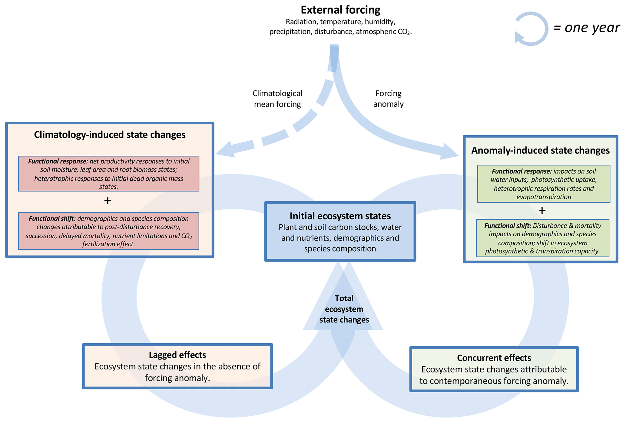
Figure 1Conceptual figure denoting annual ecosystem state changes attributable to concurrent and lagged effects. Throughout a 1-year cycle (circular arrows), lagged effects amount to the sum of ecosystem state changes induced by a reference climatological mean forcing, and concurrent effects amount to ecosystem state changes solely attributable to a contemporaneous forcing anomaly. The total state changes resulting from both concurrent and lagged effects will in turn determine the next year's initial ecosystem states.
2.2 Model and drivers
We use the DALEC model (Williams et al., 2005) to represent the principal terms and major pathways of the terrestrial C cycle. The DALEC model family has been extensively used to diagnose terrestrial C cycle dynamics across a range of site-level and spatially resolved approaches (Fox et al., 2009; Rowland et al., 2014; Bloom et al., 2016; Smallman et al., 2017; Exbrayat et al., 2018; amongst several others). Here we use DALEC version 2a (henceforth DALEC2a): a summary of the DALEC2a states and processes is depicted in Fig. 2. For the sake of brevity, we solely report changes in reference to DALEC2 (previously described by Bloom et al., 2016) and refer the reader to the Supplement (and references therein) for a complete description of the model.
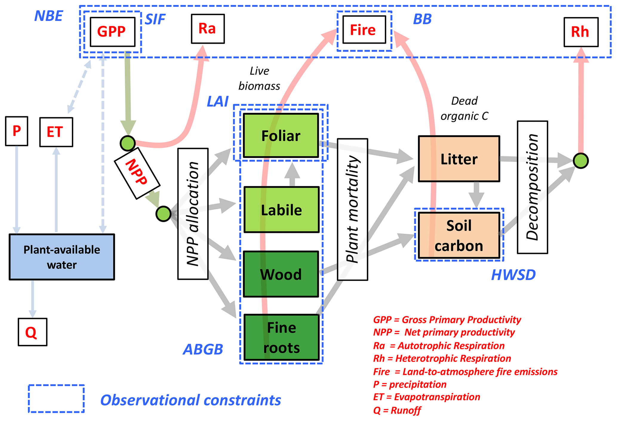
Figure 2Schematic of the CARbon DAta-MOdel fraMework (CARDAMOM) Bayesian model–data fusion approach: the DALEC2a model (described in Sect. 2.2) represents the ecosystem C and plant-available H2O balance; the dashed blue boxes denote the observational constraints used in this study (see Table 1 for abbreviations and details). The solid lines denote C and H2O fluxes between pools and/or external gains and losses. CARDAMOM is implemented at a resolution across the tropics (30∘ S–30∘ N). Within each grid cell, DALEC2a model parameters and initial ecosystem states are optimized using an adaptive Metropolis–Hastings Markov chain Monte Carlo algorithm.
We extended the DALEC2 structure to include the first-order plant-available water (H2O) pool, where the hydrological balance is defined as the sum of precipitation inputs (P) and evapotranspiration (ET) and runoff (R) outputs. In turn, the plant-available H2O limits gross primary productivity through conservation of the inherent water-use efficiency (Beer et al., 2009), where ET is calculated as a function of gross primary production (GPP) and atmospheric vapour pressure deficit (Appendix B1). Effectively, the interaction between plant-available H2O, GPP and ET constitutes a first-order plant–soil carbon–water feedback. We further appended the DALEC2 structure by including a parameterization of soil moisture limitation on heterotrophic respiration (Appendix B2), given that heterotrophic respiration dependence on soil moisture remains highly uncertain (Moyano et al., 2013; Sierra et al., 2015) as well as a dominant source of uncertainty amongst terrestrial C models (Falloon et al., 2011; Exbrayat et al., 2013a, b).
Given a range of in situ and continental-scale studies highlighting the uncertainties of fire combustion factors across a range of ecosystems (Ward et al., 1996; Bloom et al., 2015), the errors involved in representing fine-scale fire-type variability (Giglio et al., 2013), and spatial variability of fuel loads, we optimize fire C pool combustion factors (in contrast, combustion factors were prescribed as constants in Bloom et al., 2016): specifically, we optimize the combustion factors of foliar biomass (πfoliar), non-foliar biomass pools (πnfb), soil C (πSOM) and the fire resilience factor (we approximate the litter C combustion factor as the arithmetic mean of πfoliar and πSOM, given that the DALEC2a litter pool represents both above-ground and below-ground C reservoirs). Prior ranges for all π and the fire resilience are conservatively defined as spanning 0.01 to 1. We implement the ecological and dynamic constraints (Bloom and Williams, 2015) to ensure that foliar C combustion factors are greater than both non-foliar biomass and soil C combustion factors (πfoliar > πnfb and πfoliar > πSOM), which are comprehensively consistent with detailed measurements of C pool combustion factors across a range of ecosystem fire types (Shea et al., 1996; Araújo et al., 1999; van Leeuwen et al., 2014; amongst others). Finally, we also represent the uncertainty in the longevity of plant labile C; specifically, we now optimize – rather than prescribe – the labile C lifespan used during leaf flushing in DALEC2a (previously all labile C was used during leaf flush; see Bloom and Williams, 2015). The updated model structure is depicted in Fig. 2. We henceforth summarize the dynamical description of DALEC2a as
where xt represents the ecosystem state vector at time t, Mt represents the corresponding meteorological and disturbance forcings (namely monthly temperature, precipitation, global radiation, vapour pressure deficit, burned area and atmospheric CO2), p represents a vector of time-invariant process parameters and DALEC2a represents the DALEC2a operation on states xt throughout time . In summary, DALEC2a optimizable quantities consist of 26 process parameters, p, and seven initial ecosystem states (C and H2O pools; Fig. 2) at time step t=0, x0. For the sake of brevity, we include a complete description of DALEC2a state variables, process parameters and diagnostic C fluxes in the Supplement, except where an explicit mention is necessary in the paper.
2.3 Observations
The observations assimilated into CARDAMOM are summarized in Table 1. Following Bloom et al. (2016) we assimilate Moderate Imaging Spectroradiometer (MODIS) leaf area index (LAI) soil organic matter (SOM) from the Harmonized World Soil Database (HWSD; Hiederer and Köchy, 2011) and above- and below-ground biomass (ABGB, Saatchi et al., 2011). Solar-induced fluorescence (SIF) – retrieved from the Greenhouse Gases Observing Satellite (GOSAT) – is a robust proxy for photosynthetic activity: while non-linear inter-relationships at plant level and flux-tower level have been observed under certain conditions (Verma et al., 2017; Magney et al., 2017), GPP is observed to be linearly inter-related to SIF at ecosystem and regional scales (Frankenberg et al., 2011; Sun et al., 2017). Given that SIF : GPP linear relationships are known to vary substantially across individual species and entire ecosystems, here we solely assume that monthly SIF provides a constraint on the relative temporal variability of GPP (following MacBean et al., 2018). The monthly averaged 2010–2015 SIF values were derived with the polarizations and selection criteria described by Parazoo et al. (2014). The assimilation of relative SIF variability is described in Sect. 2.4.
Table 1Observational constraints assimilated into the CARDAMOM simulation.
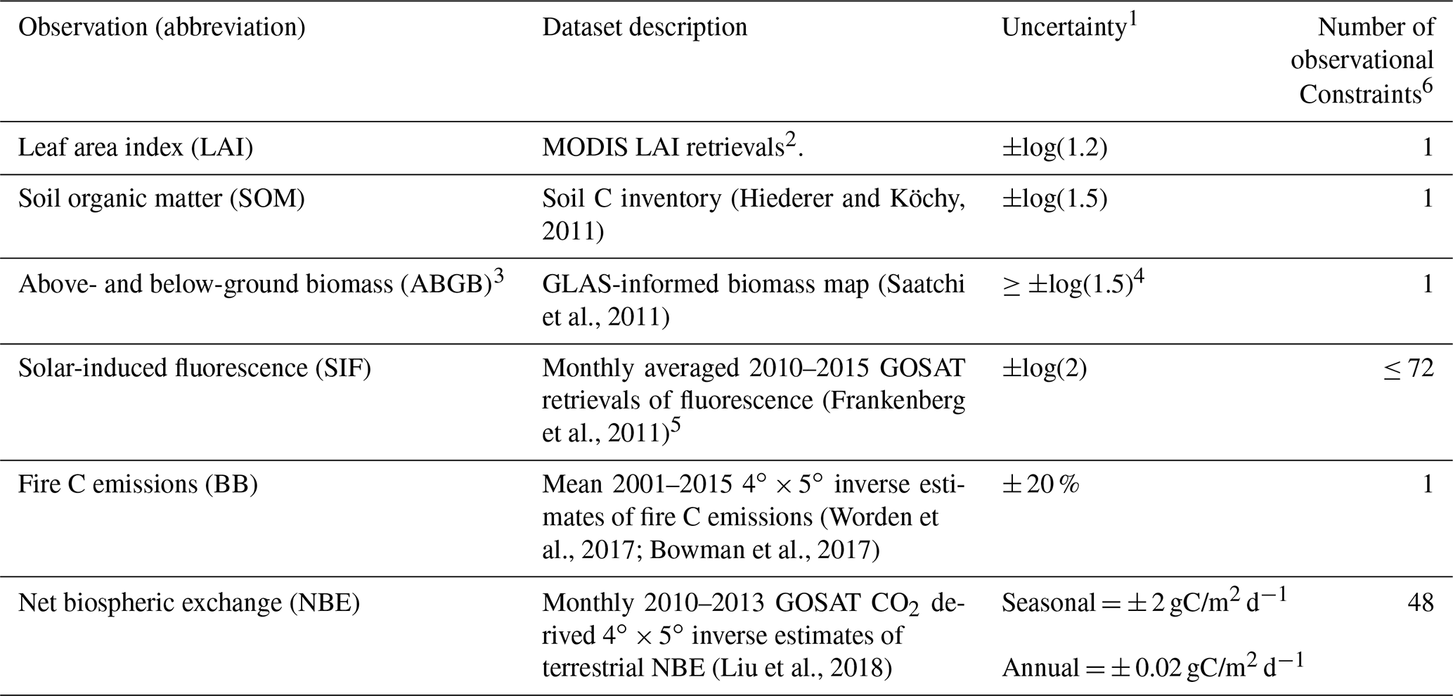
1 Uncertainties denoted as ±log() indicate log-transformed model and observed quantities (i.e. m and o in Eq. 4). 2 Only mean 2001–2015 LAI is assimilated into CARDAMOM, in order to mitigate the influence of seasonal LAI retrieval biases (Bi et al., 2015). 3 The ABGB estimate is applied as a constraint on the sum of all CARDAMOM live biomass pools (Fig. 1). 4 See Bloom et al. (2016) for details on biomass uncertainties. 5 Time-resolved SIF is assimilated as a relative constraint on the temporal variability of GPP (see Sect. 2.4). 6 See Fig. S1 for observational constraint spatial coverage.
We assimilate the GOSAT-derived 2010–2013 net biospheric C exchange (NBE) dataset (NBE > 0 for a net biosphere-to-atmosphere flux) estimated using the Carbon Monitoring System Flux atmospheric CO2 inversion framework (CMS-Flux; Liu et al., 2014, 2018). In summary, total monthly surface CO2 fluxes were scaled using a Bayesian 4D variational (4D-Var) inversion approach in order to minimize differences between GOSAT 2010–2013 observations and CMS-Flux representations of total column CO2 (we refer the reader to Liu et al., 2018, for additional details on the derivation of surface CO2 fluxes). Following Liu et al. (2017) and Bowman et al. (2017), we subtract prior estimates of anthropogenic CO2 emissions from total CMS-Flux total CO2 flux estimates, and we assume that prior anthropogenic CO2 emissions errors are minimal compared to the biospheric CO2 fluxes, given that these are typically much smaller than natural CO2 fluxes at a resolution across the tropics. We withhold 2015 CMS-Flux NBE estimates – constrained by Orbiting Carbon Observatory (OCO-2) total column CO2 observations (Liu et al., 2017) – to validate CARDAMOM 2015 regional NBE estimates and their associated uncertainties in the absence of CO2 constraints (OCO-2 NBE estimates are therefore withheld from the CARDAMOM NBE assimilation step described in Sect. 2.4); in effect, we employ the validation of CARDAMOM NBE predictions against the withheld data effect as a means of evaluating the mechanistic representations of CARDAMOM's time-varying C cycle processes.
Finally, we assimilate mean 2001–2015 fire C emission estimates derived from monthly satellite-based estimates of fire CO emissions (Jiang et al., 2017; Worden et al., 2017; Bloom et al., 2019): the estimates of biomass burning CO emissions were derived based on an ensemble of atmospheric CO inversions of column CO measurements from the Measurements of Pollution in the Troposphere (MOPITT) instrument onboard the NASA EOS/TERRA satellite (Deeter et al., 2014). We refer the reader to Jiang et al. (2017) for the details of the atmospheric CO inversion using the GEOS-Chem adjoint model and to Worden et al. (2017) for the attribution of optimized CO fluxes to biomass burning. Biomass burning CO emission estimates by Worden et al. (2017) were then used to derive total biomass burning C emissions based on monthly estimates of CO2 : CO; the approach is detailed in Bowman et al. (2017). We note that NBE estimates exhibit substantial spatial error covariance structures across individual grid cells, and the effective information content of the NBE inversions is larger than the resolution. To mitigate the spatial error correlation features identified in the NBE dataset (Bowman et al., 2017; Liu et al., 2017), we employed a 3×3 grid-cell smoothing window for monthly NBE estimates, following the approach by Liu et al. (2018).
2.4 Model–data fusion
Within each grid cell, the C cycle dynamics in DALEC are a function of meteorological and disturbance drivers M, model parameters p and initial conditions x0 (as summarized in Eq. 1). We use a Bayesian inference formulation to independently retrieve the optimal distribution of x0 and p given observations O for each grid cell, where
y is the control vector {x0,p}, p(y) is the prior probability distribution of y, and p(O|y) is proportional to the likelihood of y given O, L(y|O). At any given grid cell, the observation vector O consists of LAI, SOM, ABGB, SIF, NBE and CO-derived fire CO2 emissions (henceforth OLAI, OSOM, OABGB, OSIF, ONBE, and OCO, respectively), and – assuming errors are uncorrelated – the overall likelihood of y given O can be expressed as
For LAI, SOM, ABGB and CO, we derive the corresponding likelihood function L∗ (i.e. LLAI, LSOM, LABGB and LCO, respectively) as follows:
where oi and mi(y) correspond to the ith observation and corresponding modelled quantity derived from control vector y, respectively; σi represents the combined errors of model and data, namely the combined effects of DALEC model structural error, model driver errors and observation errors. In contrast to Bloom et al. (2016), given that MODIS LAI retrievals have exhibited systematic seasonal biases across the wet tropics (Bi et al., 2015), we solely use mean LAI as a constraint on the mean DALEC2a LAI values (therefore, for the derivation of LLAI, m and o in Eq. (3) correspond to the 2001–2015 mean modelled and observed LAI).
To constrain the relative variability of GPP based on SIF without imposing constraints on the absolute GPP magnitude, we derive LSIF – based on Eq. (4) – by formulating m and o as follows:
where SIFi and GPPi are SIF and corresponding DALEC2a GPP values at time index i and and are the corresponding means during the 2010–2015 time period.
We constrain CARDAMOM NBE using monthly CMS-Flux NBE estimates, derived from GOSAT atmospheric total column CO2 retrievals (Liu et al., 2018) spanning 2010–2013. At each location, we define the LNBE as the product of mean annual NBE and seasonal NBE anomalies using the following equation:
where denotes the annual mean DALEC2a NBE value for year a and denotes DALEC2a NBE seasonal deviations from their annual means; specifically, for a given month i with corresponding year a,
where NBEi,a is the DALEC2a NBE; observations and were derived identically to and . Similarly to Desai (2010), we implement the likelihood function outlined in Eq. (7) in order to capture both the seasonal and inter-annual modes of NBE variability; we found that solely minimizing the monthly NBE residuals following the formulation based on Eq. (4) led to disparate inter-annual variations between the model and observation-constrained NBE. Effectively the formulation in Eq. (7) – in comparison to Eq. (4) – increases the relative weight of mean annual CMS-Flux NBE constraints on DALEC2a NBE.
The uncertainty for each observational constraint (i.e. σ values in Eqs. 4 and 7) implicitly represents the combined impacts of observational random errors, systematic errors, and model structural error. In the absence of knowledge on the relative roles of observation errors in the monthly observation uncertainties and explicit knowledge of model structural error, we prescribed σ values through trial and error in order to (a) ensure that model states and diagnostic variables capture the predominant variability of the observational constraints O while (b) ensuring that σ values are comparable to the observational uncertainty. For all land surface variables (namely LAI, ABGB, SOM and SIF), m and o were log-transformed (following Bloom et al., 2016). For the mean 2001–2015 LAI constraint, we assumed log-normal uncertainty of log(1.2); we prescribed a log(2) log-normal uncertainty structure for each SIF observation. We approximated the uncertainty of the CO-derived mean 2001–2015 fire C values as %, which is broadly consistent with the monthly CO uncertainty estimates and the corresponding CO2 : CO uncertainty estimates reported by Bowman et al. (2017) and Worden et al. (2017). For NBE we prescribed and gC/m2 d−1; we found that these were suitable for capturing the first-order 2010–2013 seasonal and inter-annual components of continental-scale NBE variability. The uncertainties assumed for each observational constraint are summarized in Table 1; we note that these implicitly include the combined assumption about observational random errors, systematic errors, and model structural error. We discuss the potential impacts of observation uncertainty assumptions and make recommendations for future efforts in Sect. 3.3.
To retrieve the distribution of p(y|O), we employed an adaptive Metropolis–Hastings Markov chain Monte Carlo (MHMCMC) approach following Bloom et al. (2016) to sample the objective function, namely the product of p(y) and p(O|y); for reference, we list the individual components of the objective function in the paper's Supplement (Sect. S3). We generally found that the computational costs required to meet the MHMCMC convergence criterion reported by Bloom and Williams (2015) for each grid cell were prohibitively expensive. We updated the adaptive MHMCMC to the Haario et al. (2001) MHMCMC approach, where the MHMCMC proposal distribution is adapted as a function of previously accepted samples (see Haario et al., 2001, for algorithm details). We ran four adaptive MHMCMC chains for 108 iterations in each ∘ grid cell. We found that the latter half of the chains converged within a Gelman–Rubin convergence criterion value of < 1.2 in 75 % of the grid cells. For the subsequent analysis, we use a subset of 500 samples of y from the latter half of each MHMCMC chain, totalling 4×500 samples of y per grid cell.
2.5 Dynamical formulation of concurrent and lagged effects
Here we present a dynamical formulation for the derivation of concurrent and lagged effects on the inter-annual ecosystem state changes. To explicitly quantify the concurrent effects and lagged effects, we define the trajectory of the modelled dynamic state variables x at year a+1 as
where the state vector xa+1 – which is comprised of DALEC2a states at the beginning of year a+1 – is computed from the DALEC2a model operator D(), which is a function of the previous state xa at the beginning of year a, the meteorological and disturbance forcing history of the previous year Ma, and time-invariant ecosystem parameters p. We note that Eq. (10) is resolved on an annual time step; however, the DALEC2a operator time step is monthly, hence the operator in Eq. (10) is a composite of monthly operators as denoted in Eq. (1). To isolate the role of concurrent meteorological and disturbance anomalies in Ma, we define the C trajectory under a reference climatological mean forcing M′ as
Here we define M′ as the monthly climatological mean of the 2001–2015 meteorological and disturbance drivers and δMa as the corresponding anomaly in year a, where
With Eqs. (10) and (11), we can define the change in the state x in year a, δxa, as
This formulation allows us to define the lagged effect on ecosystem states in year a as
the concurrent effect on ecosystem states in year a as
and the sum of concurrent and lagged effects in Eqs. (14) and (15) as
We conceptually illustrate the derivation of annual concurrent and lagged effects on a given ecosystem state x in Fig. 3. Under a climatological mean forcing (blue line), the ecosystem state trajectory – solely induced by lagged processes – would diverge from an externally forced ecosystem state trajectory (black line) and would eventually converge to an equilibrium state or oscillate about a domain of attraction (Fig. 3a). For a 1-year time span, the change in ecosystem state x throughout year a, δxa, can be decomposed into a climatology-induced lagged effect change and an anomaly-induced concurrent effect change (Fig. 3a, inset).
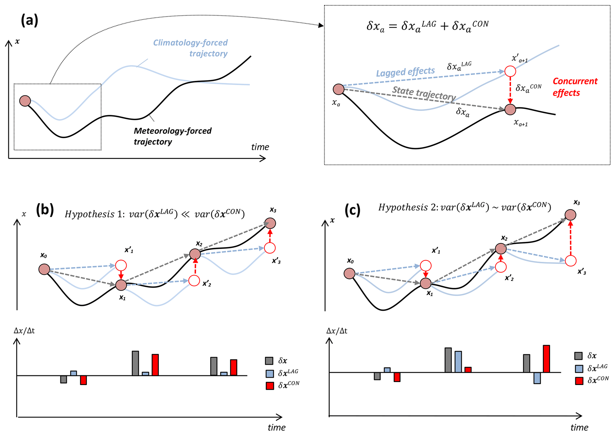
Figure 3(a) Schematic of meteorology-forced trajectory of ecosystem state x (solid black line) and trajectory of x under a climatological mean forcing (light blue solid line). Inset: state trajectory (δxa), decomposed as the sum of climatology-induced lagged effect vector () and anomaly-induced concurrent effect vector (). (b) Hypothetical scenario depicting approximately time-invariant annual lagged effects δxLAG (blue dashed arrows), in reference to changes in transient states x0, x1, x2, etc.; the temporal changes in x for each time interval, δx, δxLAG and δxCON, are shown in the underlying bar chart. In this scenario, δxLAG is relatively constant and its variability (denoted as “var()” in the schematic equation) is negligible relative to δxCON. (c) Hypothetical scenario depicting time-varying annual lagged effects δxLAG, in reference to transient states x0, x1, x2, etc.; in this scenario, the variability of δxCON is comparable to the variability of δxLAG.
From a mechanistic standpoint, the variability of is independent of meteorological forcing anomalies and is therefore solely dependent of all ecosystem states xa. For example, in a hypothetical scenario where a climatological mean forcing induces no net ecosystem state changes, and δx= δxCON. In a more general scenario, for all a: in this instance is non-zero but largely insensitive to variations in xa within a typical range of ecosystem states x; therefore, (i) the year-to-year variability of δx is largely dependent on the variability of δxCON and (ii) δxLAG amounts to an approximately constant offset term (Fig. 3b). Alternatively, if δxLAG is sufficiently sensitive to the variability of x, the variability of δx will be a function of both δxLAG and δxCON: in this instance, year-to-year variations in x are influencing both the sign and magnitude of lagged effects (Fig. 3c).
Here we investigate the possible contributions of the annual variability of δxCON and δxLAG to δx for the 2001–2015 time period across tropical ecosystems. Specifically, we test the following two hypotheses.
-
Hypothesis 1: var(δxLAG)≪ var(δxCON). In this instance, the impact of M′ on x is largely independent of the variability of x; consequently the year-to-year variability of the lagged effect force δxLAG is relatively small, and the year-to-year changes in ecosystem states, δx, are dominated by δxCON (Fig. 3b).
-
Hypothesis 2: var(δxLAG) ∼ var(δxCON). In this instance, the impact of M′ on x is dependent on the variability of x; consequently, the year-to-year variability of the lagged effects δxLAG is substantial, and the year-to-year changes in ecosystem states, δx, are substantially attributable to both δxCON and δxLAG (Fig. 3c).
The mechanistic nature of the DALEC2a model within CARDAMOM (namely the representation of allocation fractions, residence times, meteorological sensitivities and explicit representation of dynamical states) allows for a data-constrained probabilistic assessment of the relative role of lagged and concurrent effects on net ecosystem state changes. The disaggregation of δxa into and (and the associated hypotheses 1 and 2) can be projected onto any subset of net ecosystem fluxes or additive combination of gross fluxes. For example, the NBE in year a (NBEa) corresponds to the net C loss between xa and xa+1; in turn, NBEa can be decomposed into its lagged effect component (NBE) and the concurrent effect component (NBE), where
NBEa and NBE can be directly calculated from ) and ), respectively, and NBE is calculated as NBEa–NBE. By definition in the DALEC2a model, NBE is the sum of primary productivity (NPP), heterotrophic respiration (RHE) and fire (FIR) fluxes, where
In turn, disaggregation of RHE, FIR and NPP into their respective concurrent and lagged components gives
To diagnose relative inter-annual variations of a given flux F (namely the 2001–2015 time series of NBE, RHE, FIR and NPP), we derive annual anomalies ΔF relative to the mean 2001–2015 flux , where, for a given year a,
The Δ operation in Eq. (21) can be implemented in each term in Eqs. (18)–(20) without loss of equivalence between the left-hand and right-hand sides (for example, ).
Finally, we diagnose the 2001–2015 variability as a function of the inter-annual anomalies in individual ecosystem states, , relative to the mean ecosystem state . For DALEC2, these consist of annual anomalies in initial C and H2O states (see Fig. 2). For a given year, the total NBE lagged effect anomaly, , can be decomposed into
represents the NBE lagged effect component solely attributable to an anomaly in ecosystem state n (Δxa(n)), and ΔIa collectively accounts for the contribution of higher-order interactions between individual ecosystem states. In other words, given that is solely attributable to variability of annual initial conditions xa, the decomposition of to individual pool contributions provides a first-order attribution of lagged effect IAV to underlying C and H2O pool dynamics. The derivation of Eq. (22) is explicitly described in Appendix C.
To derive uncertainty estimates for each annual flux Fa or corresponding anomaly ΔFa, we calculate each term based on the 2000 samples of y at each grid cell (see Sect. 2.4), and we calculate the corresponding median and inter-quartile range (25th–75th percentiles) for each term. Inter-annual variations in 2001–2015 F and ΔF time series are reported as standard deviations of median values. We conservatively assume that F and ΔF errors are fully correlated when propagating these uncertainties across each region.
3.1 Evaluation of observation-constrained tropical C balance
Ultimately inferences about the concurrent and lagged effects on NBE can only be drawn if the CARDAMOM analysis is able to both (i) accurately represent observed NBE and (ii) accurately represent underlying states and processes controlling IAV. To assess the CARDAMOM 2001–2015 re-analysis, here we present an evaluation of CARDAMOM against (a) the assimilated 2010–2013 GOSAT-derived NBE dataset, (b) the withheld OCO-2-derived 2015 NBE dataset, and (c) assimilated and independent datasets of tropical terrestrial ecosystem states and fluxes.
Table 2CARDAMOM NBE evaluation against assimilated and predicted NBE.
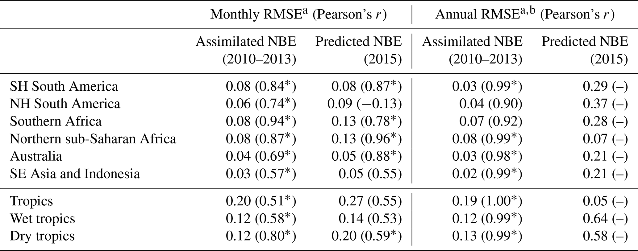
a RMSE units are PgC yr−1. b Prediction RMSE values are equivalent to absolute errors, since only one error value is considered. * Correlation p value < 0.05.
Optimized CARDAMOM NBE (a function of the optimized DALEC2a parameters and initial 2001 ecosystem states) broadly represents the monthly variability of the 2010–2013 regional-scale assimilated GOSAT-retrieved NBE (Fig. 4; Table 2). In individual regions, monthly CARDAMOM versus CMS-Flux NBE r≥0.69, with the exception of the South-East Asia and Indonesia region (r = 0.57), where the CARDAMOM and GOSAT-retrieved NBE exhibits a relatively small seasonality compared to other regions. Evaluation of CARDAMOM NBE against withheld NBE estimates from OCO-2 exhibits a degradation in the correlation and RMSE values but agrees favourably on the amplitude and timing of the NBE variability (Table 2). We find that the CARDAMOM analysis is able to robustly capture the 2010–2013 GOSAT-derived annual NBE estimates at regional scales (see Fig. 5 and Table 2; regional CARDAMOM versus CMS-Flux NBE r≥0.9). On an annual basis, all regional OCO-2 NBE estimates for 2015 except Northern Hemisphere South America are within the 90 % CARDAMOM prediction confidence intervals (Fig. 5); furthermore, all OCO-2 annual NBE estimates are within CARDAMOM 2015 prediction confidence intervals for the wet tropics, dry tropics and the entire tropical study region. We found generally lower seasonal correlations between CARDAMOM NBE and GOSAT retrieved across grid cells (Fig. S2; 25th–75th percentile = 0.19–0.63) and corresponding annual mean correlations (25th–75th percentile = 0.31–0.89) relative to the sub-continental and pan-tropical regions (Table 2); the lower correlative agreement is likely due to the limited information content of satellite-based NBE flux estimates (Liu et al., 2014; Bowman et al., 2017).
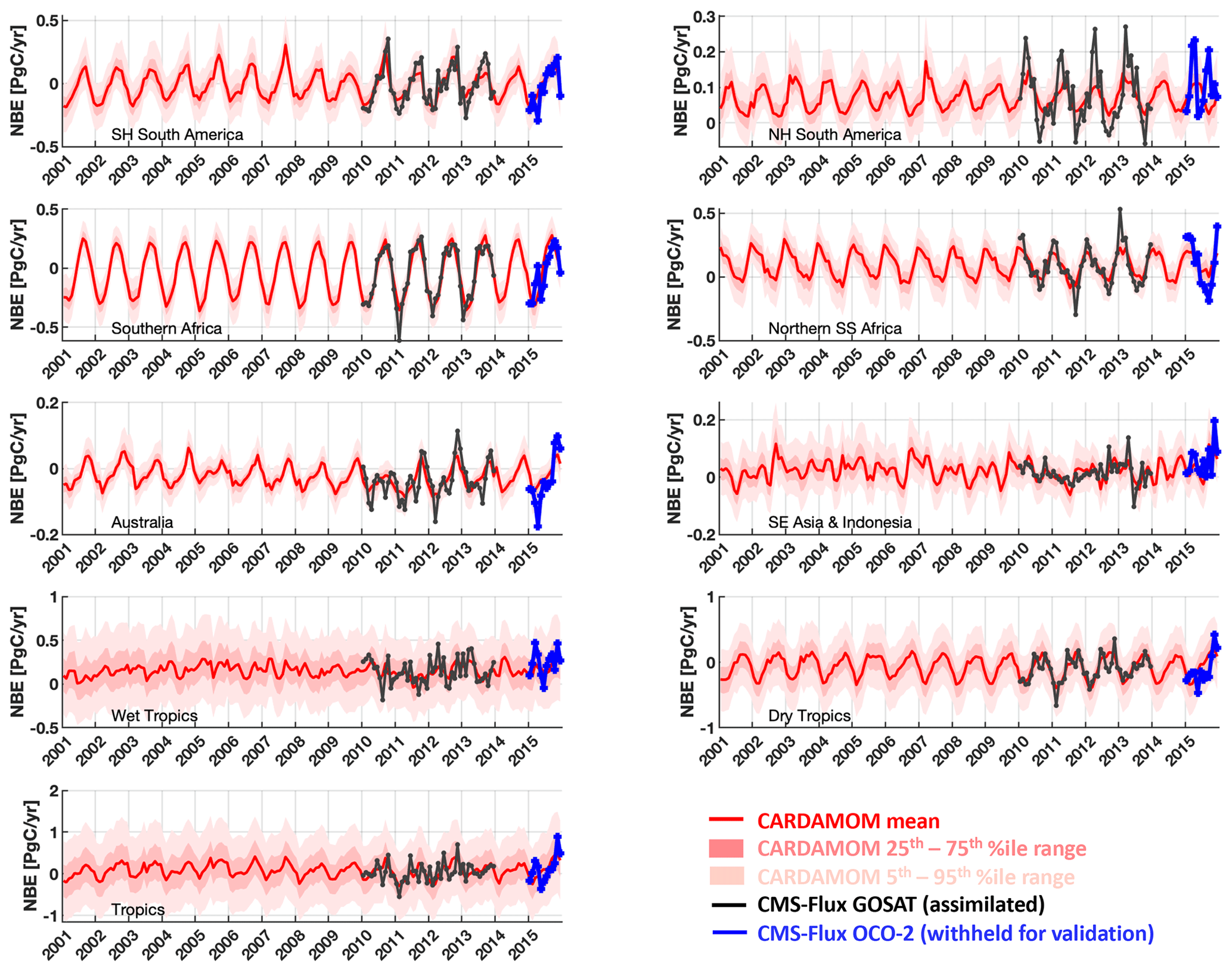
Figure 4CARDAMOM monthly analyses of 2001–2015 median NBE (red line) and associated uncertainty intervals (25th–75th percentiles in dark pink and 5th–95th percentiles in light pink). The analyses were constrained by CMS-Flux GOSAT-derived top-down fluxes (Liu et al., 2018) for the 2010–2013 period; CMS-Flux OCO-2-derived 2015 NBE fluxes were withheld for validation. The geographical definitions for each region are shown in Fig. A1 in the Appendix.
We also evaluate the 2001–2015 CARDAMOM NBE against the inter-annual variability of the NOAA ESRL surface-based global atmospheric CO2 growth rate observations (https://www.esrl.noaa.gov/gmd/ccgg/trends/, last access: 5 May 2020; see Supplement for dataset details). We assume that the atmospheric CO2 growth rate variability – once detrended to remove decadal trends in fossil fuel emissions and biogenic CO2 uptake – predominantly exhibits inter-annual variations of the tropical C balance (Baker et al., 2006; Cox et al., 2013; Sellers et al., 2018). We find that 2001–2015 detrended CARDAMOM NBE (Fig. 5, bottom-right panel) exhibits broad consistency with the atmospheric CO2 growth rate; the detrended datasets exhibit comparable levels of inter-annual variability (atmospheric CO2 growth rate IAV = ±0.62 PgC yr−1, CARDAMOM tropical NBE IAV = ±0.80 PgC yr−1) as well as a significant correlation between annual NBE growth rate anomalies (r = 0.62, pval = 0.01).
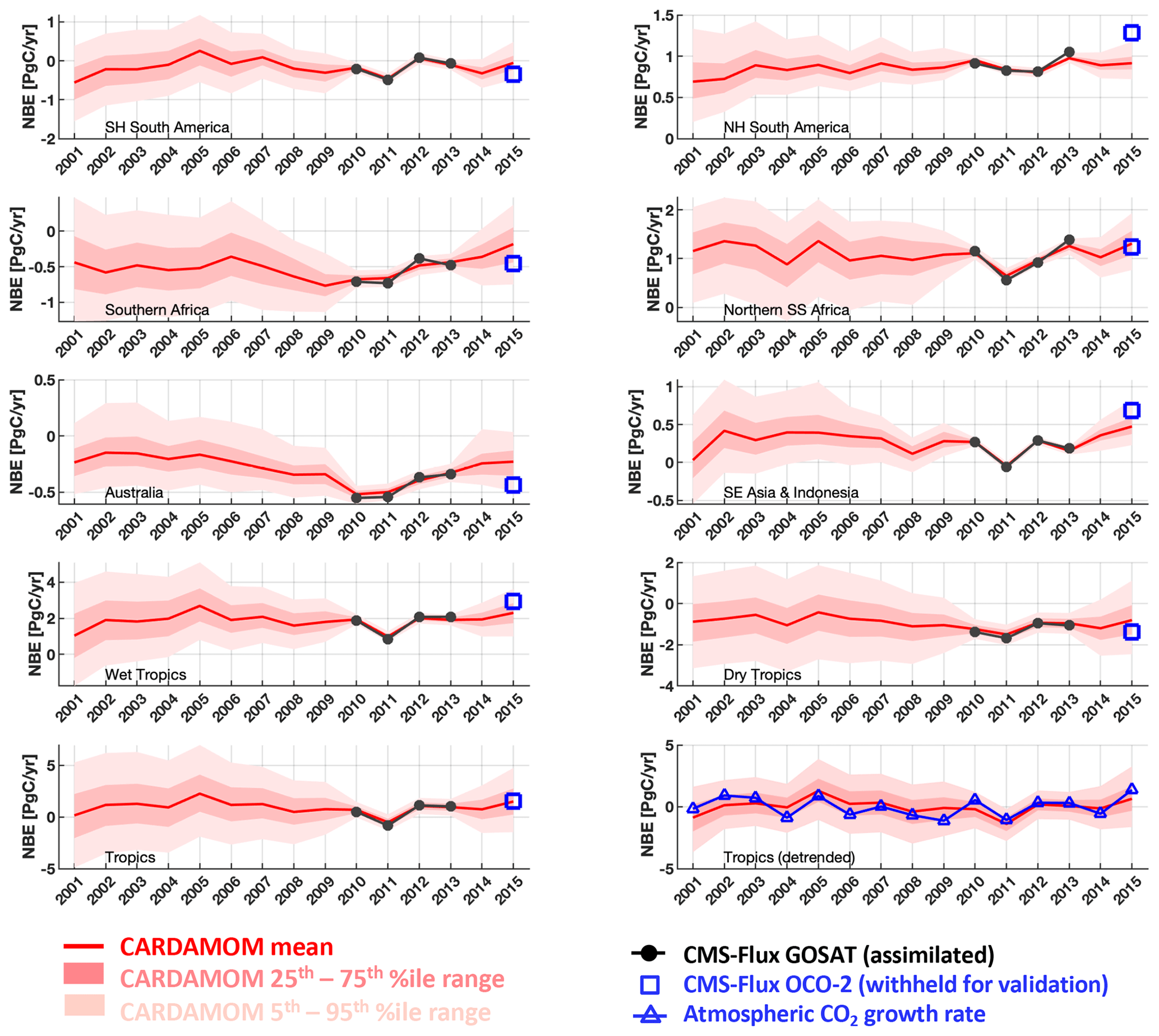
Figure 5CARDAMOM yearly analyses of 2001–2015 NBE (red line) and associated uncertainty intervals (25th–75th percentiles in dark pink and 5th–95th percentiles in light pink). The analyses were constrained by CMS-Flux GOSAT-derived top-down fluxes (Liu et al., 2018) for the 2010–2013 period. CMS-Flux OCO-2-derived 2015 NBEs (blue squares) are withheld for regional and pan-tropical NBE validation. CARDAMOM NBE and NOAA ESRL atmospheric CO2 growth rates were detrended for inter-comparison (bottom-right panel). The geographical definitions for each region are shown in Fig. A1.
The spatial variability of CARDAMOM state variables and fluxes constrained by static datasets, namely LAI, biomass, soil C and mean fire C emissions (Table 1), is broadly correlated with the observational constraints by the CARDAMOM analysis (r = 0.7–0.98; p<0.05; Fig. S2); for the above-mentioned quantities total median errors amounted to <10 %, with the exception of soil C (median error CARDAMOM soil C = 25 %). The correlation between CARDAMOM GPP and GOSAT SIF is positive and significant (p value < 0.05) in 67 % of pixels, with higher correlations in the dry tropics (25th–75th percentile = 0.41–0.78) relative to the wet tropics (25th–75th percentile = 0.13–0.63); the lower correlations in the wet tropics are generally expected, given that wet tropical ecosystems fundamentally exhibit a weaker GPP seasonal cycle.
We also evaluate the mean and inter-annual variability of CARDAMOM GPP, ET and LAI outputs against (i) two independent measurement-based GPP estimates for 2007–2015 (FLUXCOM GPP, Jung et al., 2020; and FLUXSAT GPP, Joiner et al., 2018), (ii) two independent measurement-based ET estimates (FLUXCOM ET, Jung et al., 2019; MODIS ET, Mu et al., 2011) for 2001–2013, and (iii) 2001–2015 MODIS LAI (we note that only mean 2001–2015 MODIS LAI was assimilated into CARDAMOM; see Sect. 2.3). Dataset details and regional evaluations are included Sect. S2 and Tables S2–S3 in the Supplement. In summary, we find that mean CARDAMOM pan-tropical GPP is within 20 % of both independent estimates and that regional estimates are within 40 % of both independent estimates; regional GPP IAV in CARDAMOM (0.8 %–7.4 %) is broadly consistent with FLUXSAT GPP (1.3 %–10.7 %) and FLUXCOM GPP (0.3 %–4.2 %). Pan-tropical GPP correlations are positive and significant (p value < 0.05) among all three estimates (r = 0.69–0.74); regional correlations are by and large positive but not significant. CARDAMOM mean ET values are lower but within 25 % of independent ET estimates, and differences in regional mean ET are within 50 % of independent estimates; regional ET IAV in CARDAMOM (2.3 %–5.5 %) is broadly consistent with FLUXCOM ET (0.3 %–5.9 %) and MODIS ET (1.3 %–13.4 %). Correlations between three datasets span positive and negative values but are mostly not significant; regional CARDAMOM ET correlations against MODIS and FLUXCOM (r = −0.64–0.41) are generally lower than inter-agreement between the two datasets (r = −0.27–0.94). Mean CARDAMOM LAI is within 15 % of MODIS LAI across all regions. Regional CARDAMOM LAI values (1.6 %–4.8 %) are broadly consistent with the range of MODIS LAI values (0.7 %–5.2 %); none of the regional correlation values were significant. The notable lack of correlative agreement between CARDAMOM and independent LAI and ET estimates is potentially due to (a) the lack of direct observational constraints on the temporal variability of ET and LAI in CARDAMOM, (b) systematic errors or limitations of independent LAI and ET estimation approaches on inter-annual timescales (Bi et al., 2015; Pan et al., 2020), and/or (c) fundamental limitations of CARDAMOM ET and LAI estimates (further discussed in Sect. 3.3).
Overall, we argue that (i) CARDAMOM NBE and associated uncertainties compare favourably against withheld and independent data on seasonal and inter-annual timescales, and (ii) the spatial variability and the IAV magnitude of CARDAMOM ancillary states and fluxes are in general agreement with a range of assimilated and independently estimated quantities. We discuss noteworthy caveats and limitations of retrieved CARDAMOM ecosystem dynamics – and the implications of inferred variability of concurrent and lagged effects – in Sect. 3.3. We anticipate that the ever-growing satellite CO2 record, along with increasing volume and quality of terrestrial ecosystem observations, will ultimately lead to improved seasonal and inter-annual process representations in future model–data fusion analyses of the terrestrial C balance.
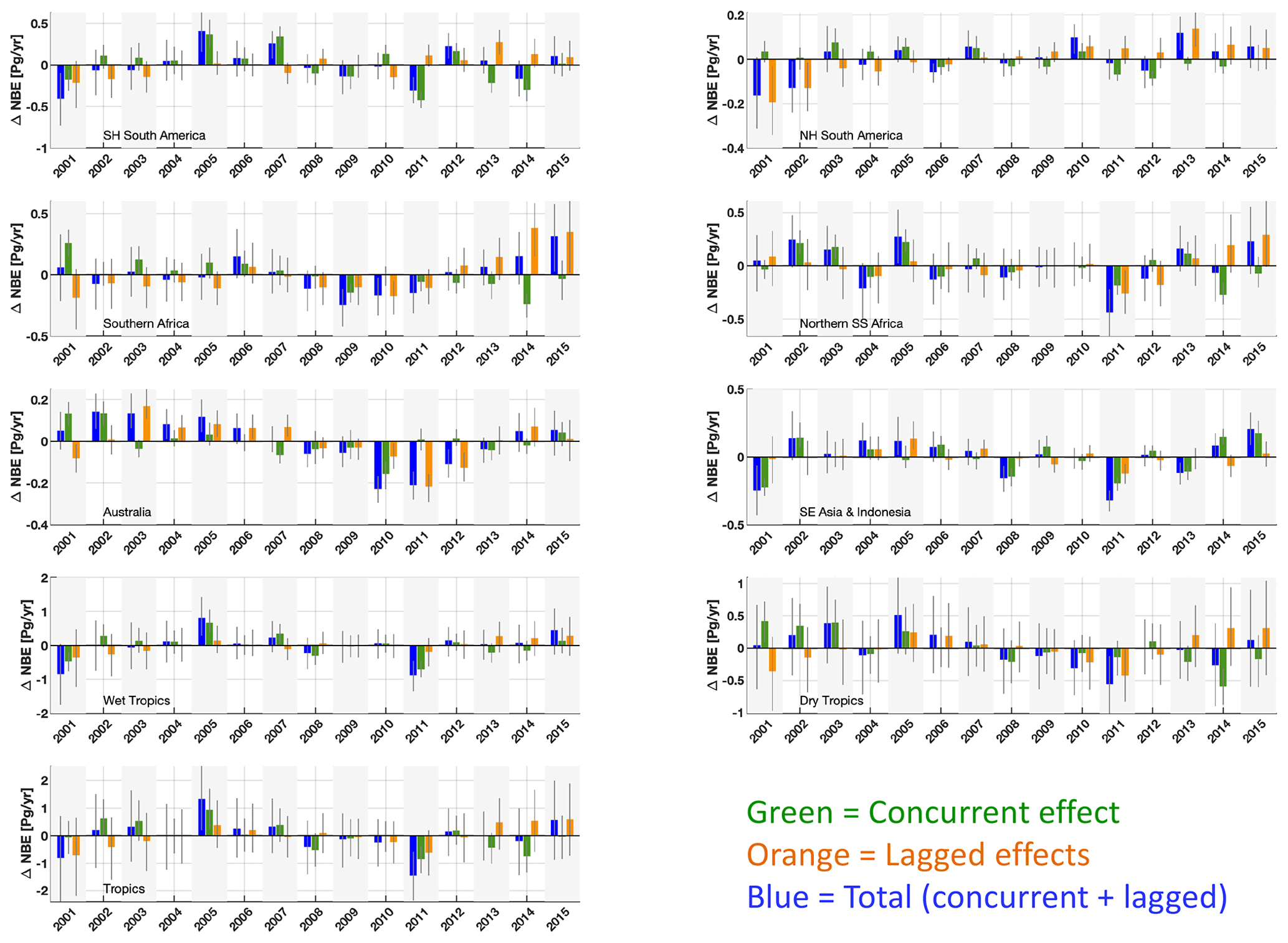
Figure 6Regional and pan-tropical median annual ΔNBE (blue bars) and its attribution to concurrent effects (ΔNBECON, green bars) and lagged effect (ΔNBELAG, orange bars) components. The geographical definitions for each region are shown in Fig. A1. Error bars denote the 25th–75th percentile uncertainty estimates for each flux anomaly.
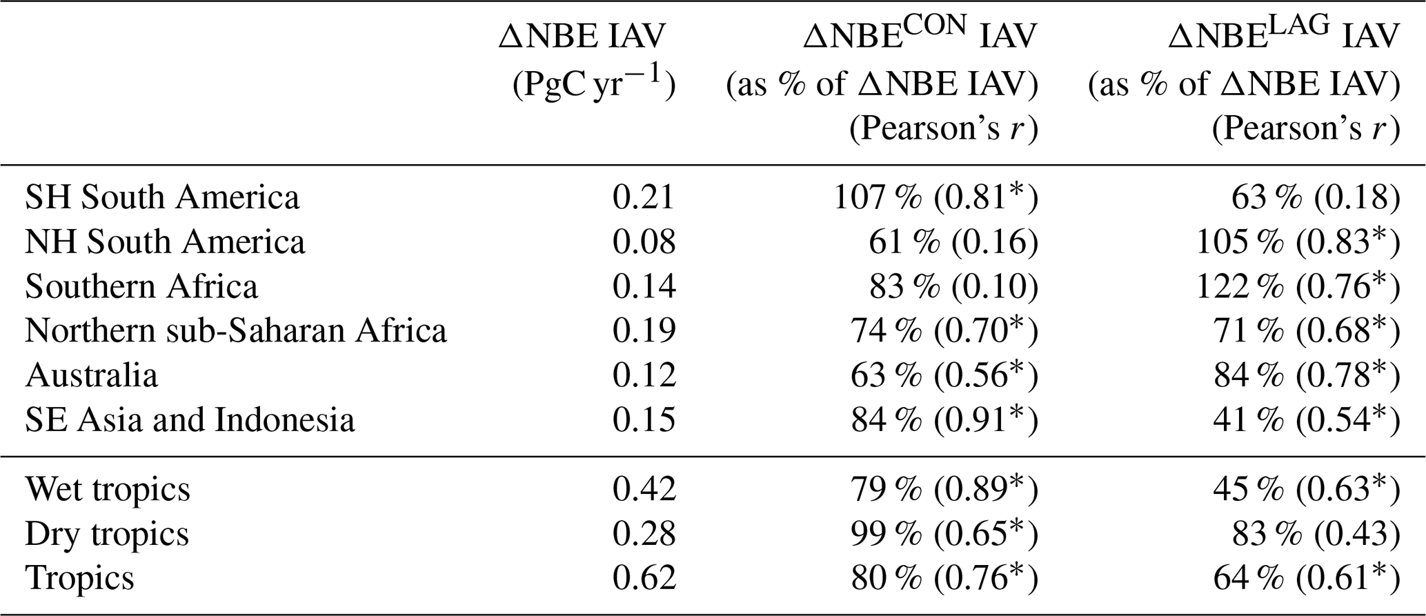
Table 32001–2015 regional ΔNBE IAV and corresponding contributions of concurrent effects (ΔNBECON) and lagged effects (ΔNBELAG); IAV values are represented here as standard deviations of annual 2001–2015 NBE values; bracketed values represent Pearson's correlation coefficients between total NBE and concurrent and lagged effect IAV. The regional masks are depicted in Fig. A1.
3.2 Concurrent and lagged effects on the tropical C balance
The attribution of annual ΔNBE into its concurrent and lagged components (ΔNBECON and ΔNBELAG) reveals that both are prominent contributors to regional and pan-tropical ΔNBE (Fig. 6). On a regional scale, ΔNBECON IAV and ΔNBELAG IAV during 2001–2015 amount to 61 %–107 % and 41 %–122 %, respectively, relative to ΔNBE IAV (Table 3). Notable ΔNBECON anomalies include (i) the positive ΔNBECON values in both South American regions during drier conditions in 2005, 2007 and 2010, in contrast with negative ΔNBECON responses during wetter conditions in 2009 and 2011, and (ii) negative ΔNBECON values during the relatively wet 2010–2011 conditions in Australia; both continental-scale responses corroborate the generally hypothesized responses of tropical ecosystems to wet and dry extreme events (Lewis et al., 2011; Bastos et al., 2013). For the most part, both ΔNBECON and ΔNBELAG contribute substantially to the year-to-year ΔNBE anomaly changes on a regional scale. Across the wet tropics, the signs of the largest ΔNBE anomalies are predominantly explained by ΔNBECON; in contrast, dry tropics ΔNBELAG IAV and ΔNBECON IAV both substantially contribute to annual ΔNBE anomalies. Instances where ΔNBELAG or ΔNBECON IAV values amount to > 100 % of ΔNBE IAV are attributable to regional and pan-tropical anti-correlations between ΔNBELAG and ΔNBECON: specifically, ΔNBELAG and ΔNBECON are anticorrelated across the tropics (r = −0.05) and all regions except SE Asia and Indonesia (r = −0.56–0.14); the consistent anticorrelation across five out of six regions suggests that lagged effects may significantly and systematically dampen the impact of ΔNBECON. On a pan-tropical scale, we found that ΔNBECON IAV and ΔNBELAG IAV are both substantial contributors to NBE IAV (80 % and 64 %); the relative importance of ΔNBELAG IAV relative to ΔNBECON is largest in the dry tropics (83 % and 99 %, respectively) and remains substantial albeit smaller in the wet tropics (79 % and 45 %, respectively). Uncertainties in ΔNBE, ΔNBECON and ΔNBELAG (Fig. 6) are generally linked to confounding NBE trend uncertainties throughout 2001–2015 (Fig. 4), particularly on a pan-tropical scale, where NBE uncertainties are considerably larger than median NBE IAV. To directly assess the uncertainty of ΔNBELAG IAV contributions to NBE IAV irrespective of annual NBE uncertainties, we (a) rank all grid-cell CARDAMOM samples by their corresponding 2001–2015 ΔNBELAG IAV and (b) combine CARDAMOM samples by ranking to generate a corresponding ensemble of regional and pan-tropical ΔNBELAG IAV estimates (summarized in Table S5). We find that the regional 95 % confidence ranges are all within 50 % of the median ΔNBELAG IAV values reported in Table 3. Notably, the ensemble of pan-tropical ΔNBELAG IAV estimates spans 42 %–97 % of NBE IAV (2.5th–97.5th percentile range), indicating that – even under overwhelmingly conservative assumptions about grid-cell ΔNBELAG IAV – lagged effects are invariably a prominent component of tropical NBE IAV.
Variations in ΔNBELAG throughout 2001–2015 include a range of lagged processes spanning between (a) ΔNBELAG changes induced by recent forcing events and (b) the gradual changes in ΔNBELAG attributable to an ecosystem's approach or oscillation around a domain of attraction (see Sect. 2.1). Notably, even in the absence of a recent forcing event, ΔNBELAG will potentially continue to change in magnitude from year to year as ecosystem states approach or oscillate around a domain of attraction. We conducted a sensitivity test for the Southern Hemisphere South America region (top-left panel of Fig. 6) to disentangle the range of contributions to 2001–2015 ΔNBELAG values: specifically, we (a) resolve ΔNBELAG in the absence of 2001–2015 forcing anomalies and (b) sequentially add 2001–2015 forcing anomalies to resolve ΔNBELAG attributable to annual forcing events (Fig. S6). In the absence of 2001–2015 forcing anomalies, lagged effects account for a ±0.11 PgC yr−1 variability in total NBE, explained by an approximately linear +0.02 PgC yr−1 increase throughout the 2001–2015 time period. The sequential addition of 2001–2015 forcing anomalies indicates the sign and magnitude of lagged effects are substantially influenced by annual forcing events; while the inter-annual variability modestly increased to ± 0.13 PgC yr−1, year-to-year changes exceed 0.3 PgC yr−1 (Fig. 6). Furthermore, while most years induced relatively short-lived (1–2-year) contributions to subsequent ΔNBELAG values, 2007 and 2010 – both notably dry years – induced more long-lasting impacts on 2010–2015 ΔNBELAG (Fig. S6). Given the combined importance of short- and long-lived impacts of forcing anomalies on lagged effects, we highlight the need to further investigate the relative contributions and potential interactions between single-event lagged effects (e.g. lagged effects attributable to a single forcing anomaly), their longevity, and their net contribution to ΔNBELAG and ΔNBE IAV.
The decomposition of ΔNBECON into constituent fluxes – namely net primary productivity (ΔNPPCON), heterotrophic respiration (ΔRHECON) and fires (ΔFIRCON) – reveals that ΔNPPCON is the largest contributor to ΔNBECON IAV (Fig. 7; Table 4), while ΔFIRCON and ΔNPPCON are comparable contributors to ΔNBECON in Australia. In Northern Hemisphere South America and South-East Asia and Indonesia, ΔRHECON variability is a smaller but substantial contributor to ΔNBECON, indicating that the integrated impacts of meteorological and disturbance forcing IAV on respiration are comparable to those on photosynthetic uptake. In Australia, the concurrent impact of fires on ΔNBECON is comparable to ΔNPPCON (Table 4). Similarly, the decomposition of ΔNBELAG into constituent fluxes (ΔNPPLAG, ΔRHELAG and ΔFIRLAG) reveals that ΔNBELAG is ubiquitously dominated by ΔNPPLAG variability, followed by modest contributions from ΔRHELAG variability and minimal contributions by ΔFIRLAG variability (see Table 4). The prominence of ΔNPPLAG is attributable to faster continental-scale response of C uptake following year-to-year variations in initial C and H2O states (relative to ΔRHELAG), indicating that live biomass dynamics (rather than dead organic C states) dominate initial ecosystem responses to external forcing anomalies. The relatively small contribution of ΔFIRLAG values to ΔNBELAG indicates that the magnitude of fires is, to first order, dominated by variability in the forcing rather than variability in fuel load within fire-prone ecosystems.
Table 4Concurrent and lagged effect NBE attributed to constituent fluxes (net primary production, heterotrophic respiration and fires, abbreviated as NPP, RHE and FIR, respectively): IAV values are represented here as the ratio of constituent flux standard deviation to NBE standard deviations of annual 2001–2015 NBE values; bracketed values correspond to Pearson's correlation coefficients between constituent flux and NBE (“*” denotes p values < 0.05). The underlined values denote the largest % IAV contribution to ΔNBECON and ΔNBELAG.
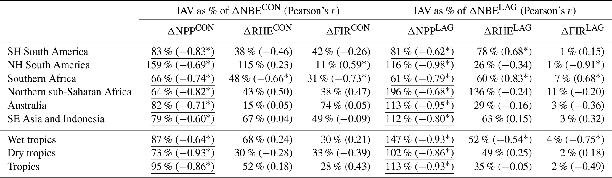
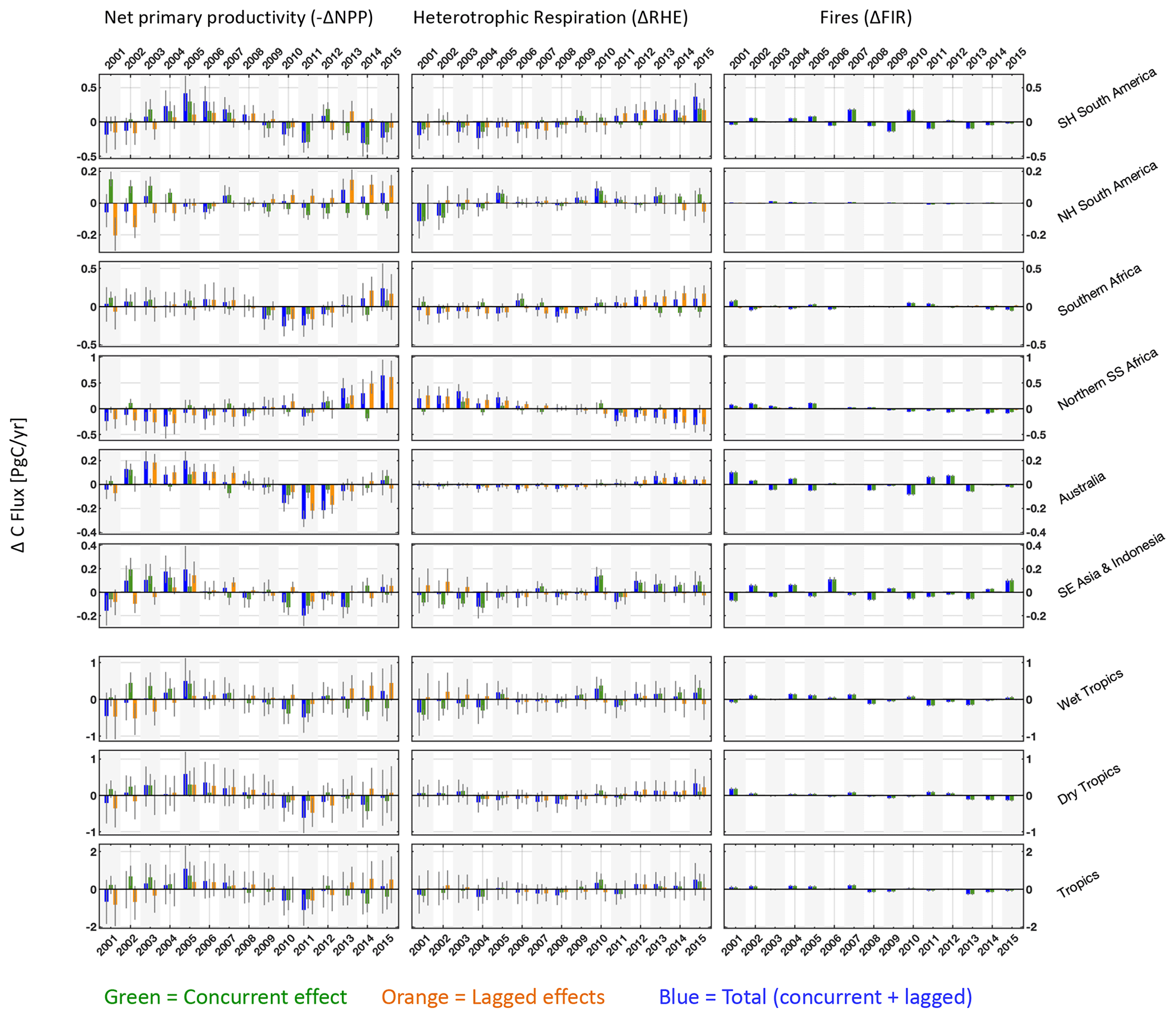
Figure 7Regional and pan-tropical median annual net primary productivity (left column), heterotrophic respiration (centre column) and fire (right column) anomalies (ΔNPP, ΔRHE and ΔFIR, respectively). Blue bars represent total anomalies and green and orange bars represent the corresponding annual concurrent and lagged effects. ΔNPP anomaly signs were reversed such that all anomalies are represented as positive for net land-to-atmosphere C flux. The sum of annual ΔNPP, ΔRHE and ΔFIR is equivalent to annual ΔNBE values presented in Fig. 6. Error bars denote the 25th–75th percentile uncertainty estimates for each flux anomaly.
We find that variability in foliar C, plant-available H2O and soil C contributes to the majority of regional and pan-tropical ΔNBELAG variability (Fig. 8). For example, both the enhanced foliar C and plant-available H2O in 2011 over the Australian continent (relative to 2010) – attributable to a combination of reduced fires and increased productivity due to anomalously wet 2010 conditions over the Australian continent (Fig. S3) – each contributed to a 0.1 PgC yr−1 net uptake increase (i.e. NBE reduction) relative to 2010. Similarly, we found that reduced foliar C in Southern Hemisphere South America following dry conditions in 2005, 2007 and 2010 induced a 0.1 PgC yr−1 NBE response in 2006, 2008 and 2011, respectively. We find that the sum of all the pool-specific ΔNBELAG anomalies approximately adds up to ΔNBELAG (Fig. S3), indicating that – insofar as these are represented in DALEC2a – ΔNBELAG is (a) to first order equivalent to the sum of NBELAG sensitivities to individual initial states and that (b) cross-pool interactions (“I” in Eq. 22) are a secondary component of ΔNBELAG. In aggregate, we find that foliar C variability contributes 41 %–120 % of ΔNBELAG variability across all regions and 58 % of the pan-tropical ΔNBELAG. Northern Hemisphere sub-Saharan Africa and South-East Asia and Indonesia are the only regions where inter-annual variations in soil C and plant-available H2O (respectively) contribute more variability than foliar C (Table 5). Notably, our results indicate that under a climatological mean forcing, (a) year-to-year changes in foliar C and plant-available H2O initial conditions are sufficient to induce substantial year-to-year changes in C uptake and (b) year-to-year changes in soil C are sufficient to substantially influence total heterotrophic respiration rates; we find that the remaining states (labile C, wood C, fine root C and litter C) explain < 0.2 PgC yr−1 variability of ΔNBELAG across all regions. We also find that the sum of regional foliar C and plant-available H2O impacts on ΔNBELAG (Fig. 8) are approximately equivalent to ΔNPPLAG (Fig. 7); in turn, the considerable contributions of both ΔNPPLAG and ΔNPPCON across tropical ecosystems indicate that both climatic variability and initial ecosystem states are substantial contributors to tropical ΔNPP IAV. Inter-annual variations of foliar C, soil C and plant-available H2O states exhibit substantial correlations with their corresponding ΔNBELAG components (Fig. S5): regional correlations are negative for foliar C (r = −0.6 to −1.0) and plant-available H2O (r = −0.7 to −0.2) and positive for soil C (r=0.6–1.0). We note that the general agreement between regional 2001–2015 foliar C IAV (1.1 %–4.0 %), CARDAMOM LAI IAV (1.6 %–4.8 %) and MODIS LAI IAV(0.7 %–5.2 %) corroborates the estimated impact of CARDAMOM C foliar dynamics on ΔNBELAG. In contrast to foliar C and plant-available H2O, soil C impacts on ΔNBELAG are predominantly induced by long-term soil C trends rather than year-to-year variability. Soil C regional trend signs (Fig. 7) are generally opposite to mean 2001–2015 NBE signs within each region (Fig. 5), indicating that the observed regional C imbalances are substantially mediated by 2001–2015 soil C trends.
Table 5IAV of 2001–2015 regional and pan-tropical NBE lagged effects attributable to annual anomalies in column-denoted ecosystem states (Eq. 22) as % of total NBE lagged effects (ΔNBELAG) IAV; bracketed values correspond to Pearson's correlation coefficients between single-state NBE lagged effects and total ΔNBELAG; “*” denotes p values < 0.05. The underlined values denote the maximum contribution in each region.
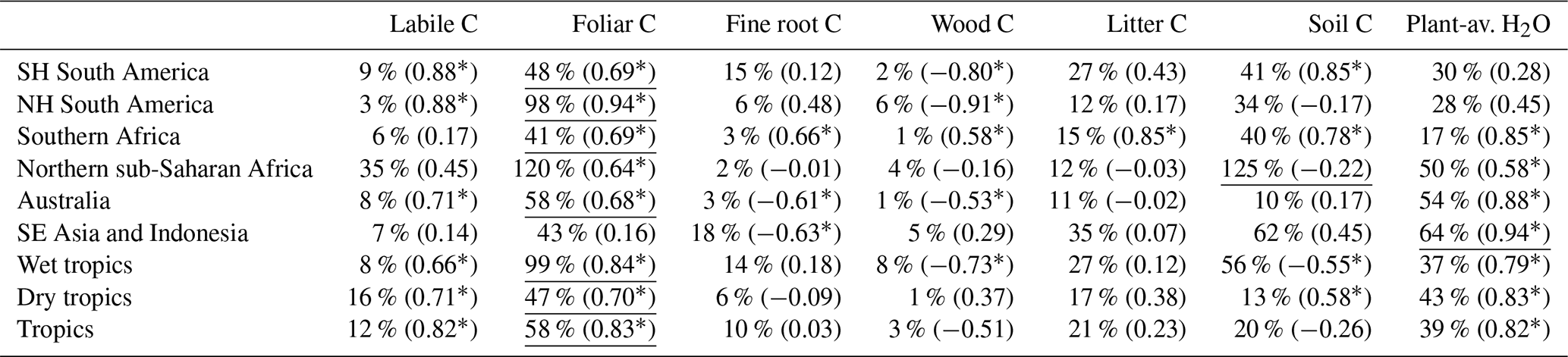
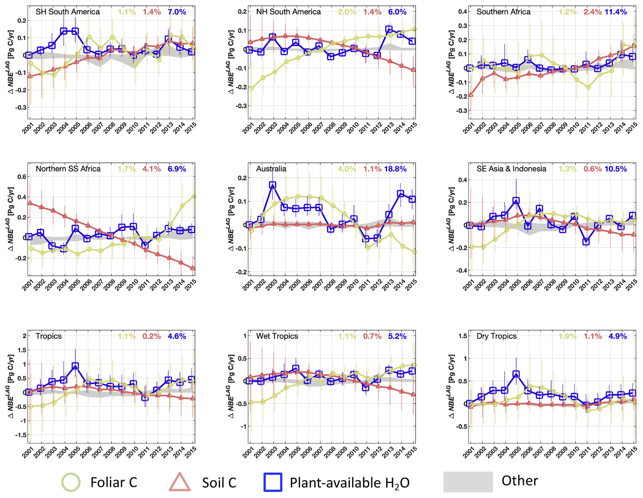
Figure 8Attribution of 2001–2015 annual regional and pan-tropical NBE lagged effect estimates (ΔNBELAG) to individual ecosystem state anomalies (i.e. the lagged effect in year a solely attributable to anomaly in ecosystem state n, ; see Eq. 22). In addition to foliar C (green circles), soil C (dark pink triangles), and plant-available H2O (blue squares), the grey areas (labelled as “Other” in the figure legend) denote the collective range of ΔNBELAG anomalies attributable to labile, wood, root and litter C. Percentage values indicate the inter-annual variability (reported as standard deviation) of median foliar C, soil C and plant-available H2O states throughout the 2001–2015 period, relative to mean 2001–2015 values within each region. The sum of annual state-specific ΔNBELAG values is approximately equal to the ΔNBELAG (see Fig. S4). Error bars denote the 25th–75th percentile uncertainty estimates for each flux anomaly.
Overall, our results indicate that (i) ΔNBELAG IAV is a prominent component of NBE IAV across tropical ecosystems; (ii) ΔNBELAG IAV is largely mediated by changes in ecosystem NPP capacity (ΔNPPLAG IAV); and (iii) ΔNPPLAG variability is regulated by inter-annual variations in ecosystem canopy and plant-available H2O states. In other words, our results highlight that inter-annual changes in ΔNBE – regardless of external forcing anomalies – are substantially determined by inter-annual anomalies in ecosystem H2O and canopy states. Lagged heterotrophic respiration responses (ΔRHELAG) are mediated by soil C states changes and are secondary component of NBE IAV; the dampened role of ΔRHELAG (relative to ΔNPPLAG) is likely due to the inherent lags between biomass growth and subsequent mortality inputs to soil C states, combined with ∼ 5–50-year mean dead organic C residence times across tropical ecosystems (Bloom et al., 2016). The relative importance of NPP-mediated lagged effects in responses to climatic anomalies has also been inferred on from in situ and continental-scale measurements (Sherry et al., 2008; Detmers et al., 2015; Wolf et al., 2016). Our findings also suggest that tracking the long-term evolution of tropical ecosystem canopy cover (Saatchi et al., 2013; Shi et al., 2017) and reducing the process-level uncertainties associated with foliar C dynamics relationships to meteorological and disturbance forcings (discussed in Sect. 3.3) are potentially critical for advancing process-level understanding of tropical NBE IAV. We anticipate that continued monitoring of NBE (e.g. following the 2015–2016 ENSO event) and subsequent attribution to concurrent and lagged effects will also be critical to better quantify the longevity NPP recovery (e.g. Schwalm et al., 2017) and to improve confidence in characterizing concurrent and lagged NPP impacts on the tropical C balance. Finally, while our analysis is focused on the ΔNBELAG sensitivity to year-to-year ecosystem state changes, we note that the magnitude of ΔNBECON is also in principle dependent on time-varying ecosystem states (Fig. 1); we recognize that further investigation on whether ΔNBECON IAV is (a) predominantly sensitive to forcing anomalies, or (b) sensitive to year-to-year ecosystem state changes, could amount to a critical step towards accurately characterizing the climate sensitivity of ΔNBE.
3.3 Observation and model uncertainty caveats
The prescribed observation uncertainty characteristics (Table 1) are potentially a critical source of error in the data-informed representation of terrestrial C cycle dynamics and its subsequent partitioning into concurrent and lagged effects. For example, relative differences in the mean NBE values retrieved from aircraft and satellite CO2 measurements over the Amazon Basin (Alden et al., 2016; Bowman et al., 2017) highlight the need to determine the sensitivity of our results to top-down estimates of NBE. While the uncertainty structures of top-down CO2 inversion estimates are beyond the scope of our paper, we recognize the need to robustly assess and characterize uncertainties in seasonal and inter-annual variations in NBE. Potential limitations in the linear SIF : GPP assumption include (i) systematic underestimations of afternoon GPP stress, given that the GOSAT overpass time is ∼ 1 pm, and (ii) uncharacterized biases emerging from non-linear SIF : GPP under extreme conditions (Verma et al., 2017). We highlight that recent efforts to merge multiple SIF datasets (Zhang et al., 2018) and process-based representations of SIF : GPP (Bacour et al., 2019) can together be used to improve the accuracy of SIF : GPP representation in CARDAMOM. We also note that the CARDAMOM likelihood function (Eq. 3) fundamentally assumes all errors are independent; however, commonalities in the derived datasets – such as systematic representation errors across all datasets and transport errors in the GEOS-Chem-derived CO2 and CO emissions – may lead to unrepresented error correlations in the likelihood functions.
We generally acknowledge that more elaborate approaches and a more comprehensive treatment of model and data error characteristics are necessary to understand the contribution of individual data stream error (Keenan et al., 2011; Heald et al., 2004; MacBean et al., 2016, 2018). Specifically, the explicit and accurate representation of model structural error is critical for both accurate retrievals of physical parameters and accurate model predictions (Brynjarsdottir and O'Hagan, 2014) and solving for error model parameters (Schoups and Vrugt, 2010; Xu et al., 2017) is potentially advantageous for physical parameter retrievals and prediction purposes. For example, we note that without an error model structure we cannot explicitly account for cross-correlations in the errors between observations or the impacts of heteroscedasticity (Schoups and Vrugt, 2010). While the identification and optimization of an appropriate structural error model are beyond the scope of this paper, we highlight that this as an important priority for future CARDAMOM analyses.
Unrepresented processes DALEC2a model structure – particularly processes that are potentially substantial contributors to ΔNBECON and ΔNBELAG – amount to an additional source of uncertainty in our analysis. Potentially critical processes include time-varying autotrophic respiration (Rowland et al., 2014), plant C allocation and plant mortality, as well as explicit representation of coarse woody debris (Smallman et al., 2017). In particular, given that our results suggest that foliar C is a major contributor to ΔNBE, unrepresented processes relating to tropical leaf phenology may substantially impact the accuracy of lagged effect attribution, including phenological processes regulating leaf onset, leaf lifespan and litterfall seasonality (Chave et al., 2010; Caldararu et al., 2012; Xu et al., 2016), as well as the time-varying allocation regimes (Doughty et al., 2015). Furthermore, while the DALEC2a phenology assumes a time-invariant ratio between LAI and foliar C (i.e. a time-invariant ecosystem-level leaf carbon mass per area), the joint roles of leaf demographics and species distribution on the temporal variability of leaf carbon mass per area could potentially amount to a significant impact on photosynthetic capacity, and subsequently on the variability of ΔNBECON and ΔNBELAG. We also highlight year-to-year changes in species composition (such as C3 : C4 plants) and the temporal dynamics of vegetation and soil nutrients as potential contributors to ΔNBELAG (Sherry et al., 2008; Schimel et al., 1997) are potentially unrepresented but critical processes, particularly in fire-prone regions (Pellegrini et al., 2018) and nutrient-limited tropical forest ecosystems (Wieder et al., 2015). A potential limitation in CARDAMOM ET estimates is the assumed inherent water-use efficiency relationship between GPP, ET and VPD (Eq. B4); recent efforts (Zhou et al., 2015; Boese et al., 2017) advocate for improved parameterizations for semi-empirical GPP : ET relationships, which could ultimately impact the sign and magnitude of inter-annual CARDAMOM ET variations – and the associated plant-available H2O balance – across tropical ecosystems. Finally, we highlight the need to investigate the sensitivity of our results to the 2001–2015 climatological mean forcing: while to first order the diagnosis of lagged effect anomalies from the mean (rather than absolute values) are insensitive to the reference forcing, further efforts are required to determine whether non-linear impacts of an alternative reference forcing (e.g. a climatological mean forcing based on a 30-year climate normal) may amplify or dampen ΔNBELAG IAV estimates.
Our continental-scale results indicate that DALEC2a model complexity is adequate to both represent NBE variability and accurately predict NBE outside the training window on a pan-tropical scale (2015), which provides a first-order assessment of the adequacy of the DALEC2a model structure. A notable exception is the substantial underestimation of CARDAMOM 2015 NBE within the Northern Hemisphere South America region (Fig. 5); given the considerable impact of the 2015 ENSO event within the region (Liu et al., 2017), the biased CARDAMOM NBE prediction suggests that either (a) the DALEC2a model structure cannot adequately represent NBE responses to climatic extremes or (b) the 2010–2013 NBE observational constrains are insufficient to accurately inform the regional DALEC2a states and process parameters. To determine the relative impact of model error, we anticipate that additional insights could be obtained by retrieving ΔNBECON and ΔNBELAG based on alternative DALEC model structures (Fox et al., 2009; Smallman et al., 2017). The implementation of DALEC2a assimilation and prediction evaluation across long-term records eddy covariance CO2 and H2O fluxes would amount to a useful evaluation of the model structure constrained by multiple data streams (e.g. following Richardson et al., 2010; Keenan et al., 2013; Smallman et al., 2017), and the potential sensitivities of ΔNBECON and ΔNBELAG to underlying model structures. While there are currently few tropical ecosystem sites where multi-year NBE constraints are available, we highlight that the analysis of ΔNBECON and ΔNBELAG at eddy covariance sites would also benefit from the relative wealth of ancillary site-level repeat measurements of C and H2O states and fluxes, and would ultimately allow more in-depth evaluation and hypothesis tests on lagged effect processes and their role on ΔNBE dynamics. Finally, to diagnose the potential role of higher-order process interactions on lagged and concurrent effects – such as nutrient limitations, ecosystem demography and explicit representations of carbon–water–energy interactions – we highlight that the ΔNBECON and ΔNBELAG attribution methodology introduced here can in principle be applied using higher complexity terrestrial biosphere models (e.g. Huntzinger et al., 2013, 2017; Macbean et al., 2018; Longo et al., 2019).
The prominent role of ΔNBELAG across the tropics throughout 2001–2015 supports our second hypothesis (Sect. 2.5), namely that concurrent and lagged effect variations are comparable on inter-annual timescales. By constraining a diagnostic ecosystem C balance model with an array of terrestrial C cycle observations (LAI, biomass, soil C, SIF, CO-derived fire C emissions and CO2-derived NBE), we show that on annual timescales both ΔNBECON and ΔNBELAG effects are substantial contributors to the 2001–2015 tropical C balance. The IAV of ΔNBECON is largely accounted for by NPP, with sizeable fire contributions from Australia, South-East Asia, Indonesia and South America and heterotrophic respiration contributions from wet tropical ecosystems. ΔNBELAG variability is overwhelmingly dominated by the impact of inter-annual variations in lagged NPP effects, followed by a modest contribution from the state dependence of heterotrophic respiration. In aggregate, anomalies in foliar C, plant-available H2O, and soil C were identified as the primary influences on ΔNBELAG variability. Our findings therefore highlight a critical need to explicitly account for lagged effects when investigating the process-level tropical NBE responses to climatic variability on inter-annual timescales. Furthermore, our findings highlight the need to accurately and continuously resolve NBE at sub-continental scales in order to advance our mechanistic and process-level understanding of terrestrial C cycling and its evolving sensitivity to climate.
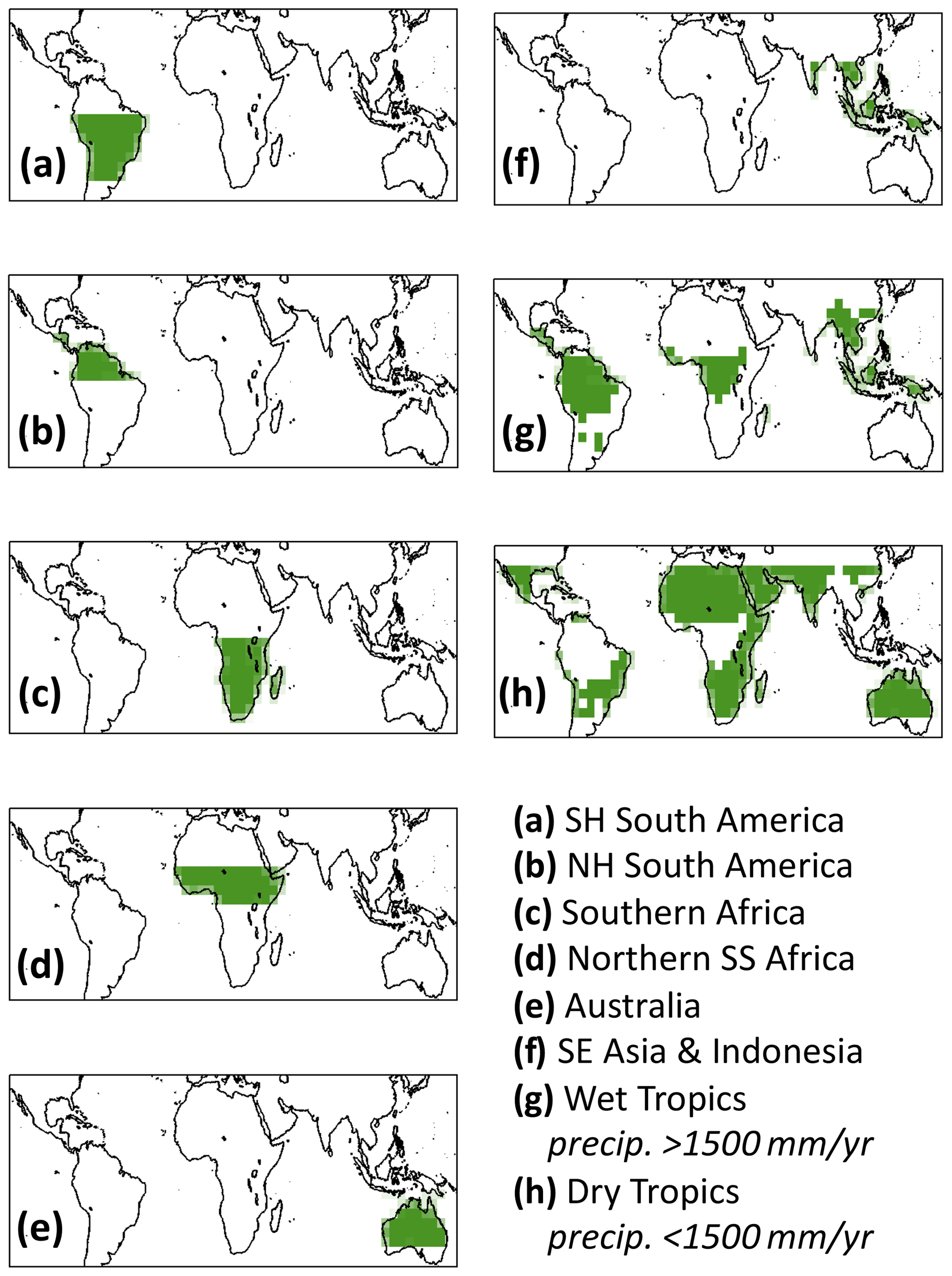
Figure A1Regional masks used in this study. The 1500 mm yr−1 precipitation thresholds were based on the ERA-Interim mean annual precipitation rates throughout the 2001–2015 study period.
The following sections provide a summary of the process parameterizations introduced in the DALEC version implemented in the Bloom et al. (2016) study. For completeness, a full description of DALEC2a is provided in the paper's Supplement.
B1 DALEC2a water balance and GPP water stress
The DALEC2a plant-available water balance at time step t+1 is derived as
where W denotes total plant-available H2O (in mm H2O storage equivalent) and P, R and ET precipitation, runoff and evapotranspiration fluxes (mm d−1) over the time period Δt (d). We note that this equation represents a water balance in the dynamic plant-available H2O pool and does not include deep groundwater, confined aquifers or other unconnected/static storages. Following a generalized non-linear reservoir formulation, we parameterize monthly runoff losses as a second-order decay function with respect to storage, Wt, as
where α is a second-order decay constant (mm−1 d−1). The dependence of runoff on W2 – instead of W – ensures that the fractional rate of plant-available H2O loss is proportional to W; relative to a first-order linear kinetics model, this provides a better representation of faster relative plant-available H2O depletion following high precipitation events, followed by slower losses during lower precipitation time spans (e.g. Matteucci et al., 2015) and serves a functional approximation of both storage-excess and infiltration-excess runoff generation mechanisms in most cases. Following previous results from land surface model development experiments (e.g. Liang et al., 1994; Lawrence et al., 2011), we assume that net runoff inputs from adjacent pixels are a negligible term in the lumped grid-scale H2O budget at spatial resolution. By construction, Rt values predicted at are unphysically high ), while loss rates at produce implausibly low residual storage (Wt−RtΔt) values. Therefore, in the eventuality of , we calculate runoff as , effectively representing a storage-excess overflow mechanism by introducing a transition between a state-dependent regime to a direct runoff regime.
We apply a linear scaling on GPP with respect to the plant-available H2O, where
where ω represents the plant-available H2O stress threshold; Eq. (B3) effectively imposes a stress factor on GPP spanning between 0 and 1, and offers a simplified representation of the integrated effects of leaf–soil H2O potential differences and their impact on canopy conductance. Evapotranspiration at time t is derived as
where υe is the inherent water-use efficiency (Beer et al., 2009) and VPD is the vapour pressure deficit derived from ERA-Interim monthly reanalysis datasets. Equations (B1)–(B4) amount to a plant–water feedback parameterization, and together represent a reduced complexity version of the DALEC water module implemented by Spadavecchia et al. (2011). All parameters involved in the above-mentioned parameterization – namely α, υe, ω and W0 – are optimized along with other DALEC2a parameters in CARDAMOM; the prior ranges are described in Table S1.
B2 Heterotrophic respiration
We parameterize the meteorological dependence of heterotrophic respiration ρ at time t as follows:
where T and P represent the monthly temperature and precipitation vectors. We chose to use P as a driver for heterotrophic respiration sensitivity to moisture, given that (a) the majority of heterotrophic respiration is expected to occur in the near-surface soil layer, and (b) near-surface soil moisture strongly covaries with P – rather than water storage – at monthly timescales. Previous versions of DALEC solely parameterized ρt as a function of temperature (e.g. Bloom et al., 2016 and references therein); effectively, the formulation in Eq. (B5) induces a joint sensitivity to relative changes in both temperature and near-surface moisture. The prior ranges for the respiration temperature and precipitation sensitivity parameters (Θ and sp) are reported in Table S1.
In the DALEC2a representation of the ecosystem C balance, the state vector xa consists of the C and H2O pool values at the start of year a. To diagnose the sensitivity of 2010–2015 lagged effects to the variability of ecosystem states, we conduct a sensitivity analysis to explicitly quantify the impact of individual ecosystem state anomalies – relative to their 2010–2015 mean values – on the variability of δxLAG throughout 2010–2015. To do this, we define the anomaly of the nth individual state in year a as the sum of finite differences relative to the mean state:
where is an N-element vector of the mean 2010–2015 states; N is the number of model state variables; xa(n) is an N-element vector of ecosystem states, where for the ith element xa(n)(i)=xa(i) for i = n, and for i≠n. Based on Eqs. (11) and (14), we can derive the state change under a climatological mean forcing of each term in Eq. (C1), and therefore
Ia collectively accounts for the unaccounted contribution of higher-order interactions between individual pool anomalies [ on . As outlined in Sect. 2.5, the “δx” terms in Eq. (C2) can be mapped onto any DALEC2a flux variable; specifically, NBE can be defined as the sum of lagged effect NBE components attributable to and as follows:
and can be directly calculated from ) and ), respectively. More succinctly, we summarize Eq. (B3) as
where represents the lagged effect anomaly attributable solely to the initial condition anomaly in ecosystem state n. By applying the “Δ” operator (Eq. 21) on Eq. (C3), Eq. (C4) can alternatively be expressed as
Effectively, the lagged effect partitioning formulation outlined in Eq. (C5) allows us to quantitatively diagnose the NBE lagged effect dependence on the inter-annual dynamics of individual C and H2O states depicted in Fig. 2.
ECMWF re-analysis datasets were obtained from https://www.ecmwf.int/en/forecasts/datasets/reanalysis-datasets/era-interim (Berrinsford et al., 2011). Burned area was obtained from https://globalfiredata.org/pages/data/ (Giglio et al., 2013). MODIS LAI data were obtained from https://e4ftl01.cr.usgs.gov/MOLT/ (Myneni et al., 2015). CMS-Flux datasets are available at cmsflux.jpl.nasa.gov. Biomass is available from Sassan Saatchi (sasan.s.saatchi@jpl.nasa.gov) upon reasonable request. The HWSD soil data was obtained from https://esdac.jrc.ec.europa.eu/content/global-soil-organic-carbon-estimates (Hiederer and Kochy, 2012). Gridded GOSAT fluorescence datasets used in this analysis are available from Nicholas Parazoo (nicholas.c.parazoo@jpl.nasa.gov) upon reasonable request. Biomass burning CO fluxes data was obtained from https://dashrepo.ucar.edu/dataset/CO_Flux_Inversion_Attribution.html (Bloom et al., 2019). FLUXCOM datasets were obtained from https://www.bgc-jena.mpg.de/geodb/ (Jung 2018, Jung 2020). FLUXSAT data were obtained from https://avdc.gsfc.nasa.gov/pub/tmp/FluxSat_GPP/ (Joiner et al., 2018). MODIS ET data are available from http://files.ntsg.umt.edu/data/NTSG_Products/MOD16/ (Running, 2020). The NOAA ESRL dataset was obtained from https://www.esrl.noaa.gov/gmd/ccgg/trends/ (Dlugokencky and Tans, 2020). The CARDAMOM results presented throughout the paper are available upon request.
The supplement related to this article is available online at: https://doi.org/10.5194/bg-17-6393-2020-supplement.
AAB, KWB, JL, AGK, and DSS designed the research, AAB conducted the analysis, and all the co-authors extensively contributed to evaluation of results and writing of the manuscript.
The authors declare that they have no conflict of interest.
Part of this work was carried out at the Jet Propulsion Laboratory, California Institute of Technology, under a contract with the National Aeronautics and Space Administration (NASA). Part of this study was funded as a component of NERC's support of the National Centre for Earth Observation. SSS and AGK were also supported by NASA through the Earth Science Program. We are thankful for feedback from Michael Keller, Paul Levine, Marcos Longo, Shuang Ma and Alexander Norton. The NCAR MOPITT project is supported by the National Aeronautics and Space Administration (NASA) Earth Observing System (EOS) Program. The MOPITT team is grateful for the contributions of COMDEV and ABB BOMEM with support from the Canadian Space Agency (CSA), the Natural Sciences and Engineering Research Council (NSERC) and Environment Canada.
This research was supported by a NASA Earth Sciences grant (no. NNH16ZDA001N-IDS).
This paper was edited by Andreas Ibrom and reviewed by two anonymous referees.
Ahlström, A., Raupach, M. R., Schurgers, G., Smith, B., Arneth, A., Jung, M., Reichstein, M., Canadell, J. G., Friedlingstein, P., Jain, A. K., Kato, E., Poulter, B., Sitch, S., Stocker, B. D., Viovy, N., Wang, Y. P., Wiltshire, A., Zaehle, S., and Zeng, N.: The dominant role of semi-arid ecosystems in the trend and variability of the land CO2 sink, Science, 348, 895–899, 2015.
Alden, C. B., Miller, J. B., Gatti, L. V., Gloor, M. M., Guan, K., Michalak, A. M., van der Laan-Luijkx, I. T., Touma, D., Andrews, A., Basso, L. S., Correia, C. S. C., Domingues, L. G., Joiner, J., Krol, M. C., Lyapustin, A. I., Peters, W., Shiga, Y. P., Thoning, K., van der Velde, I. R., van Leeuwen, T. T., Yadav, V., and Diffenbaugh, N. S.: Regional atmospheric CO2 inversion reveals seasonal and geographic differences in Amazon net biome exchange, Glob. Change Biol., 22, 3427–3443, https://doi.org/10.1111/gcb.13305, 2016.
Andela, N. and van der Werf, G. R.: Recent trends in African fires driven by cropland expansion and El Niño to La Niña transition, Nat. Clim. Change, 4, 791–795, 2014.
Anderegg, W. R., Schwalm, C., Biondi, F., Camarero, J. J., Koch, G., Litvak, M., Ogle, K., Shaw, J.D., Shevliakova, E., Williams, A. P., Wolf, A., Ziaco, E., and Pacala, S.: Pervasive drought legacies in forest ecosystems and their implications for carbon cycle models, Science, 349, 528–532, 2015.
Araújo, T. M., Carvalho Jr., J. A., Higuchi, N., Brasil Jr., A. C. P., and Mesquita, A. L. A.: A tropical rainforest clearing experiment by biomass burning in the state of Pará, Brazil, Atmos. Environ., 33, 1991–1998, 1999.
Arnone, J. A., Verburg, P. S. J., Johnson, D. W., Larsen, J. D., Jasoni, R. L., Lucchesi, A. J., Batts, C. M., von Nagy, C., Coulombe, W. G., Schorran, D. E., Buck, P. E., Braswell, B. H., Coleman, J. S., Sherry, R. A., Wallace, L. L., Luo, Y., and Schimel, D. S.: Prolonged suppression of ecosystem carbon dioxide uptake after an anomalously warm year, Nature, 455, 383–386, https://doi.org/10.1038/nature07296, 2008.
Bacour, C., Maignan, F., MacBean, N., Porcar-Castell, A., Flexas, J., Frankenberg, C., Peylin, P., Chevallier, F., Vuichard, N., and Bastrikov, V.: Improving estimates of Gross Primary Productivity by assimilating solar-induced fluorescence satellite retrievals in a terrestrial biosphere model using a process-based SIF model, J. Geophys. Res.-Biogeo., 124, 3281–3306, 2019.
Baker, D. F., Law, R. M., Gurney, K. R., Rayner, P., Peylin, P., Denning, A. S., Bousquet, P., Bruhwiler, L., Chen, Y. H., Ciais, P., and Fung, I. Y.: TransCom 3 inversion intercomparison: Impact of transport model errors on the interannual variability of regional CO2 fluxes, 1988–2003, Global Biogeochem. Cy., 20, GB1002, https://doi.org/10.1029/2004GB002439, 2006.
Baldocchi, D., Chu, H., and Reichstein, M.: Inter-annual variability of net and gross ecosystem carbon fluxes: A review, Agr. Forest Meteorol., 249, 520–533, 2017.
Bastos, A., Running, S. W., Gouveia, C., and Trigo, R. M.: The global NPP dependence on ENSO: La Niña and the extraordinary year of 2011, J. Geophys. Res.-Biogeo., 118, 1247–1255, 2013.
Beer, C., Ciais, P., Reichstein, M., Baldocchi, D., Law, B. E., Papale, D., Soussana, J. F., Ammann, C., Buchmann, N., Frank,D., Gianelle, D., Janssens, I. A., Knohl, A., Koestner, B., Moors, E., Roupsard, O., Verbeeck, H., Vesala, T., Williams, C. A., and Wohlfahrt, G.: Temporal and among-site variability of inherent water use efficiency at the ecosystem level, Global Biogeochem. Cy., 23, GB2018, https://doi.org/10.1029/2008gb003233, 2009.
Beer, C., Reichstein, M., Tomelleri, E., Ciais, P., Jung, M., Carvalhais, N., Rödenbeck, C., Arain, M. A., Baldocchi, D., Bonan, G. B., Bondeau, A., Cescatti, A., Lasslop, G., Lindroth, A., Lomas, M., Luyssaert, S., Margolis, H., Oleson, K. W., Roupsard, O., Veendendaal, E., Viovy, N., Williams, C., Woodard, F. I., and Papale, D.: Terrestrial gross cabon dioxide uptake: Global distribution and covariation with climate, Science, 329, 834–838, 2010.
Berrisford, P., Dee, D., Poli, P., Brugge, R., Fielding, K., Fuentes,M., Kallberg, P., Kobayashi, S., Uppala, S., and Simmons, A.: The ERA-Interim Archive, ERA Rep. Ser., 1, available at: https://www.ecmwf.int/node/8174 (last access: 20 July 2018), 2011.
Bi, J., Knyazikhin, Y., Choi, S. H., Park, T., Barichivich, J., Ciais, P., Fu, R., Ganguly, S., Hall, F., Hilker, T., Huete, A., Jones, M., Kimball, J., Lyapustin, A. I., Mottus, M., Nemani, R. R., Piao, S. L., Poulter, B., Saleska, S. R., Saatchi, S. S., Xu, L., Zhou, L. M., and Myneni, R. B.: Sunlight mediated seasonality in canopy structure and photosynthetic activity of Amazonian rainforests, Environ. Res. Lett., 10, 064014, https://doi.org/10.1088/1748-9326/10/6/064014, 2015
Bloom, A. A. and Williams, M.: Constraining ecosystem carbon dynamics in a data-limited world: integrating ecological “common sense” in a model–data fusion framework, Biogeosciences, 12, 1299–1315, https://doi.org/10.5194/bg-12-1299-2015, 2015.
Bloom, A. A., Worden, J., Jiang, Z., Worden, H., Kurosu, T., Frankenberg, C., and Schimel, D.: Remote sensing constraints on South America fire traits by Bayesian fusion of atmospheric and1140 surface data, Geophys. Res. Lett., 42, 1268–1274, https://doi.org/10.1002/2014GL062584, 2015.
Bloom, A. A., Exbrayat, J.-F., van der Velde, I. R., Feng, L., and Williams, M.: The decadal state of the terrestrial carbon cycle: Global retrievals of terrestrial carbon allocation, pools, and residence times, P. Natl. Acad. Sci. USA, 113, 1285–1290, https://doi.org/10.1073/pnas.1515160113, 2016.
Bloom, A., Jiang, Z., and Worden, H.: Global Carbon Monoxide (CO) Flux Estimates for 2001–2015, UCAR/NCAR – DASH Repository, https://doi.org/10.26024/r1r2-6620, 2019.
Boese, S., Jung, M., Carvalhais, N., and Reichstein, M.: The importance of radiation for semiempirical water-use efficiency models, Biogeosciences, 14, 3015–3026, https://doi.org/10.5194/bg-14-3015-2017, 2017.
Bowman, K. W., Liu, J., Bloom, A. A., Parazoo, N. C., Lee, M., Jiang, Z., Menemenlis, D., Gierach, M. M., Collatz, G. J., Gurney, K. R., and Wunch, D.: Global and Brazilian carbon response to El Niño Modoki 2011–2010, Earth Space Sci., 4, 637–660, 2017
Braswell, B. H., Schimel, D. S., Linder, E., and Moore, B. I. I. I.: The response of global terrestrial ecosystems to interannual temperature variability, Science, 278, 870–873, 1997.
Brynjarsdóttir, J. and O'Hagan, A.: Learning about physical parameters: The importance of model discrepancy, Inverse Problems, 30, 114007, https://doi.org/10.1088/0266-5611/30/11/114007, 2014.
Caldararu, S., Palmer, P. I., and Purves, D. W.: Inferring Amazon leaf demography from satellite observations of leaf area index, Biogeosciences, 9, 1389–1404, https://doi.org/10.5194/bg-9-1389-2012, 2012.
Carvalhais, N., Forkel, M., Khomik, M., Bellarby, J., Jung, M., Migliavacca, M., Mu, M., Saatchi, S., Santoro, M., Thurner, M., Weber, U., Ahrens, B., Beer, C., Cescatti, A., Randerson, J. T., and Reichstein, M.: Global covariation of carbon turnover times with climate in terrestrial ecosystems, Nature, 514, 213–217, https://doi.org/10.1038/nature13731, 2014.
Chave,J.,Navarrete,D.,Almeida,S.,Álvarez,E., Aragão,L.E.O. C., Bonal, D., Châtelet, P., Silva-Espejo, J. E., Goret, J.-Y., von Hildebrand, P., Jiménez, E., Patiño, S., Peñuela, M. C., Phillips, O. L., Stevenson, P., and Malhi, Y.: Regional and seasonal patterns of litterfall in tropical South America, Biogeosciences, 7, 43–55, https://doi.org/10.5194/bg-7-43-2010, 2010.
Chen, Y., Morton, D. C., Jin, Y., Collatz, G. J., Kasibhatla, P. S., Werf, G. R. van der, DeFries, R. S., and Randerson, J. T.: Long-term trends and interannual variability of forest, savanna and agricultural fires in South America, Carbon Manag., 4, 617–638, https://doi.org/10.4155/cmt.13.61, 2013.
Cox, P., Pearson, D., Booth, B., Friedlingstein, P., Huntingford, C., Jones, C., and Luke, C.: Sensitivity of tropical carbon to climate change constrained by carbon dioxide variability, Nature, 494, 341–344, 2013.
Deeter, M. N., Martínez-Alonso, S., Edwards, D. P., Emmons, L. K., Gille, J. C., Worden, H. M., Sweeney, C., Pittman, J. V., Daube, B. C., and Wofsy, S. C.: The MOPITT Version 6 product: algorithm enhancements and validation, Atmos. Meas. Tech., 7, 3623–3632, https://doi.org/10.5194/amt-7-3623-2014, 2014.
Desai, A. R.: Climatic and phenological controls on coherent regional interannual variability of carbon dioxide flux in a heterogeneous landscape, J. Geophys. Res.-Biogeo., 115, G00J02, https://doi.org/10.1029/2010jg001423, 2010.
Detmers, R. G., Hasekamp, O., Aben, I., Houweling, S., Leeuwen, T. T. V., Butz, A., Landgraf, J., Köhler, P., Guanter, L., and Poulter, B.: Anomalous carbon uptake in Australia as seen by GOSAT, Geophys. Res. Lett., 42, 8177–8184, https://doi.org/10.1002/2015GL065161, 2015.
Dlugokencky, E. and Tans, P.: Trends in Atmospheric Carbon Dioxide NOAA/GML; data available at https://www.esrl.noaa.gov/gmd/ccgg/trends/, last access: 5 May 2020.
Doughty, C. E., Metcalfe, D. B., Girardin, C. A. J., Amezquita,F. F., Durand, L., Huasco, W. H., Costa, M. C., Costa, A. C. L., Rocha, W., Meir, P., Galbraith, D., and Malhi, Y.: Source and sink carbon dynamics and carbon allocation in the Amazon basin, Global Biogeochem. Cy., 29, 645–655, 2015.
Exbrayat, J.-F., Pitman, A. J., Zhang, Q., Abramowitz, G., and Wang, Y.-P.: Examining soil carbon uncertainty in a global model: response of microbial decomposition to temperature, moisture and nutrient limitation, Biogeosciences, 10, 7095–7108, https://doi.org/10.5194/bg-10-7095-2013, 2013a.
Exbrayat, J. F., Pitman, A. J., Abramowitz, G., and Wang, Y. P.: Sensitivity of net ecosystem exchange and heterotrophic respiration to parameterization uncertainty, J. Geophys. Res.-Atmos., 118, 1640–1651, 2013b.
Exbrayat, J. F., Smallman, T. L., Bloom, A. A., Hutley, L. B., and Williams, M.: Inverse determination of the influence of fire on vegetation carbon turnover in the pantropics, Global Biogeochem. Cy., 32, 1776–1789, 2018.
Falloon, P., Jones, C. D., Ades, M., and Paul, K.: Direct soil moisture controls of future global soil carbon changes: An important source of uncertainty, Global Biogeochem. Cy., 25, GB3010, https://doi.org/10.1029/2010GB003938, 2011.
Fang, Y., Michalak, A. M., Schwalm, C. R., Huntzinger, D. N., Berry, J. A., Ciais, P., Piao, S. L., Poulter, B., Fisher, J. B., Cook, R. B., Hayes, D., Huang, M. Y., Ito, A., Jain, A., Lei, H. M., Lu, C. Q., Mao, J. F., Parazoo, N. C., Peng, S. S., Ricciuto, D. M., Shi, X. Y., Tao, B., Tian, H. Q., Wang, W. L., Wei, Y. X., and Yang, J.: Global land carbon sink response to temperature and precipitation varies with ENSO phase, Environ. Res. Lett., 12, 064007, https://doi.org/10.1088/1748-9326/aa6e8e, 2017.
Feng, L., Palmer, P. I., Bösch, H., Parker, R. J., Webb, A. J., Cor- reia, C. S. C., Deutscher, N. M., Domingues, L. G., Feist, D. G., Gatti, L. V., Gloor, E., Hase, F., Kivi, R., Liu, Y., Miller, J. B., Morino, I., Sussmann, R., Strong, K., Uchino, O., Wang, J., and Zahn, A.: Consistent regional fluxes of CH4 and CO2 inferred from GOSAT proxy XCH4 : XCO2 retrievals, 2010–2014, Atmos. Chem. Phys., 17, 4781–4797, https://doi.org/10.5194/acp-17-4781-2017, 2017.
Fox, A., Williams, M., Richardson, A. D., Cameron, D., Gove, J. H., Quaife, T., Ricciuto, D., Reichstein, M., Tomelleri, E., Trudinger, C. M., and van Wijk, M. T.: The reflex project: comparing different algorithms and implementations for the inversion of a terrestrial ecosystem model against eddy covariance data, Agr. Forest Meteorol., 149, 1597–1615, 2009.
Frank, D., Reichstein, M., Bahn, M., Thonicke, K., Frank, D., Mahecha, M., Smith, P., Van der Velde, M., Vicca, S., Babst, F., Beer, C., Buchmann, N., Canadell, J., Ciais, P., Cramer, W., Ibrom, A., Miglietta, F., Poulter, B., Rammig, A., Seneviratne, S., Walz, A., Wattenbach, M., Zavala, M., and Zscheischler, J.: Effects of climate extremes on the terrestrial carbon cycle: concepts, processes and potential future impacts, Glob. Change Biol., 21, 7861–2880, 2015.
Frankenberg, C., Fisher, J. B., Worden, J., Badgley, G., Saatchi, S. S., Lee, J.-E., Toon, G. C., Butz, A., Jung, M.,Kuze, A., and Yokota, T.: New global observations of the terrestrial carbon cycle from GOSAT: patterns of plant fluorescence with gross primary productivity, Geophys. Res. Lett., 38, L17706, https://doi.org/10.1029/2011GL048738, 2011.
Friedlingstein, P., Meinshausen, M., Arora, V. K., Jones, C. D., Anav, A., Liddicoat, S. K., and Knutti, R.: Uncertainties in CMIP5 climate projections due to carbon cycle feedbacks, J. Clim., 27, 511–526, 2014.
Friend, A. D., Lucht, W., Rademacher, T. T., Keribin, R., Betts, R., Cadule, P., Ciais, P., Clark, D. B., Dankers, R., Fal- loon, P. D., Ito, A., Kahana, R., Kleidon, A., Lomas, M. R., Nishina, K., Ostberg, S., Pavlick, R., Peylin, P., Schaphoff, S., Vuichard, N., Warszawski, L., Wiltshire, A., and Woodward, F. I.: Carbon residence time dominates uncertainty in terrestrial vegetation responses to future climate and atmospheric CO2, P. Natl. Acad. Sci. USA, 111, 3280–3285, https://doi.org/10.1073/pnas.1222477110, 2014.
Gatti, L. V., Gloor, M., Miller, J. B., Doughty, C. E., Malhi, Y., Domingues, L. G., Basso, L. S., Martinewski, A., Correia, C. S., C., Borges, V. F., Freitas, S., Braz, R., Anderson, L. O., Rocha, H., Grace, J., Phillips, O. L., and Lloyd, J.: Drought sensitivity of Amazonian carbon balance revealed by atmospheric measurements, Nature, 506, 76–80, https://doi.org/10.1038/nature12957, 2014.
Giglio, L., Randerson, J. T., and van der Werf, G. R.: Analysis of daily, monthly, and annual burned area using the fourth- generation global fire emissions database (GFED4), J. Geophys. Res.-Biogeo., 118, 317–328, https://doi.org/10.1002/jgrg.20042, 2013.
Guenet, B., Camino-Serrano, M., Ciais, P., Tifafi, M., Maignan, F., Soong, J. L., and Janssens, I. A.: Impact of priming on global soil carbon stocks, Glob. Change Biol., 24, 1873–1883, 2018.
Haario, H., Saksman, E., and Tamminen, J.: An adaptive Metropolis algorithm, Bernoulli, 7, 223–242, 2001.
Heald, C. L., Jacob, D. J., Jones, D., Palmer, P. I., Logan, J. A., Streets, D. G., Sachse, G. W., Gille, J. C., Hoffman, R. N., and Nehrkorn, T.: Comparative inverse analysis of satellite (MOPITT) and aircraft (TRACE-P) observations to estimate Asian sources of carbon monoxide, J. Geophys. Res.-Atmos., 109, D23306, https://doi.org/10.1029/2004JD005185, 2004.
Hiederer, R. and Köchy, M.: Global soil organic carbon estimates and the harmonized world soil database, EUR 25225 EN, Publications Office of the European Union, 79 pp., https://doi.org/10.2788/13267, 2011.
Hiederer, R. and Kochy, M.: Global Soil Organic Carbon Estimates and the Harmonized World Soil Database, EUR Scientific and Technical Research series – ISSN 1831-9424 (online), ISSN 1018-5593 (print), ISBN 978-92-79-23108-7, https://doi.org/10.2788/1326, 2012.
Holling, C. S.: Resilience and stability of ecological systems, Ann. Rev. Ecol. Syst., 4, 1–23, 1973.
Hopkins, F. M., Filley, T. R., Gleixner, G., Lange, M., Top, S. M., and Trumbore, S. E.: Increased belowground carbon inputs and warming promote loss of soil organic carbon through complementary microbial responses, Soil Biol. Biochem., 76, 57–69, 2014.
Huntzinger, D. N., Schwalm, C., Michalak, A. M., Schaefer, K., King, A. W., Wei, Y., Jacobson, A., Liu, S., Cook, R. B., Post, W. M., Berthier, G., Hayes, D., Huang, M., Ito, A., Lei, H., Lu, C., Mao, J., Peng, C. H., Peng, S., Poulter, B., Riccuito, D., Shi, X., Tian, H., Wang, W., Zeng, N., Zhao, F., and Zhu, Q.: The North American Carbon Program Multi-Scale Synthesis and Terrestrial Model Intercomparison Project – Part 1: Overview and experimental design, Geosci. Model Dev., 6, 2121–2133, https://doi.org/10.5194/gmd-6-2121-2013, 2013.
Huntzinger, D. N., Michalak, A. M., Schwalm, C., Ciais, P., King, A. W., Fang, Y., Schaefer, K., Wei, Y., Cook, R. B., Fisher, J. B., Hayes, D., Huang, M., Ito, A., Jain, A. K., Lei, H., Lu, C., Maignan, F., Mao, J., Parazoo, N., Peng, S., Poulter, B., Ricciuto, D., Shi, X., Tian, H., Wang, W., Zeng, N., and Zhao, F.: Uncertainty in the response of terrestrial carbon sink to environmental drivers undermines carbon-climate feedback predictions, Sci. Rep.-UK, 7, 4765, https://doi.org/10.1038/s41598-017-03818-2, 2017.
Jiang, Z., Worden, J. R., Worden, H., Deeter, M., Jones, D. B. A., Arellano, A. F., and Henze, D. K.: A 15-year record of CO emissions constrained by MOPITT CO observations, Atmos. Chem. Phys., 17, 4565–4583, https://doi.org/10.5194/acp-17-4565-2017, 2017.
Joiner, J., Yoshida, Y., Zhang, Y., Duveiller, G., Jung, M., Lyapustin, A., Wang, Y., and Tucker, C. J.: Estimation of terrestrial global gross primary production (GPP) with satellite data-driven models and eddy covariance flux data, Remote Sens., 10, 1346, https://doi.org/10.3390/rs10091346, 2018.
Jung, M., Reichstein, M., Schwalm, C. R., Huntingford, C., Sitch, S., Ahlström, A., Arneth, A., Camps-Valls, G., Ciais, P., Friedlingstein, P., Gans, F., Ichii, K., Jain, A. K., Kato, E., Papale, D., Poulter, B., Raduly, B., Rödenbeck, C., Tramontana, G., Viovy, N., Wang, Y.-P., Weber, U., Zaehle, S., and Zeng, N.: Compensatory water effects link yearly global land CO2 sink changes to temperature, Nature, 541, 516–520, 2017.
Jung, M.: FLUXCOM Global Land Energy Fluxes, https://doi.org/10.17871/FLUXCOM_EnergyFluxes_v1, 2018.
Jung, M.: FLUXCOM Global Land Carbon Fluxes, https://doi.org/10.17871/FLUXCOM_CarbonFluxes_v1, 2020.
Jung, M., Koirala, S., Weber, U., Ichii, K., Gans, F., Camps-Valls, G., Papale, D., Schwalm, C., Tramontana, G., and Reichstein, M.: The FLUXCOM ensemble of global land-atmosphere energy fluxes, Sci. data, 6, 1–14, 2019.
Jung, M., Schwalm, C., Migliavacca, M., Walther, S., Camps-Valls, G., Koirala, S., Anthoni, P., Besnard, S., Bodesheim, P., Carvalhais, N., Chevallier, F., Gans, F., Goll, D. S., Haverd, V., Köhler, P., Ichii, K., Jain, A. K., Liu, J., Lombardozzi, D., Nabel, J. E. M. S., Nelson, J. A., O'Sullivan, M., Pallandt, M., Papale, D., Peters, W., Pongratz, J., Rödenbeck, C., Sitch, S., Tramontana, G., Walker, A., Weber, U., and Reichstein, M.: Scaling carbon fluxes from eddy covariance sites to globe: synthesis and evaluation of the FLUXCOM approach, Biogeosciences, 17, 1343–1365, https://doi.org/10.5194/bg-17-1343-2020, 2020.
Keenan, T. F., Carbone, M. S., Reichstein, M., and Richardson, A. D.: The model–data fusion pitfall: assuming certainty in an uncertain world, Oecologia, 167, 587–597, 2011.
Keenan, T. F., Davidson, E. A., Munger, J. W., and Richardson, A. D.: Rate my data: quantifying the value of ecological data for the development of models of the terrestrial carbon cycle, Ecol. Appl., 23, 273–286, 2013.
Kurc, S. A. and Small, E. E.: Soil moisture variations and ecosystem-scale fluxes of water and carbon in semiarid grassland and shrubland, Water Resour. Res., 43, W06416, https://doi.org/10.1029/2006WR005011, 2007.
Lawrence, D. M., Oleson, K. W., Flanner, M. G., Thornton, P. E., Swenson, S. C., Lawrence, P. J., Zeng, X., Yang, Z.-L., Levis, S., Sakaguchi, K., Bonan, G. B., and Slater, A. G.: Parameterization improvements and functional and structural advances in version 4 of the Community Land Model, J. Adv. Model. Earth Sys., 3, M03001, https://doi.org/10.1029/2011MS000045, 2011.
Le Quéré, C., Moriarty, R., Andrew, R. M., Canadell, J. G., Sitch, S., Korsbakken, J. I., Friedlingstein, P., Peters, G. P., Andres, R. J., Boden, T. A., Houghton, R. A., House, J. I., Keeling, R. F., Tans, P., Arneth, A., Bakker, D. C. E., Barbero, L., Bopp, L., Chang, J., Chevallier, F., Chini, L. P., Ciais, P., Fader, M., Feely, R. A., Gkritzalis, T., Harris, I., Hauck, J., Ilyina, T., Jain, A. K., Kato, E., Kitidis, V., Klein Goldewijk, K., Koven, C., Landschützer, P., Lauvset, S. K., Lefèvre, N., Lenton, A., Lima, I. D., Metzl, N., Millero, F., Munro, D. R., Murata, A., Nabel, J. E. M. S., Nakaoka, S., Nojiri, Y., O'Brien, K., Olsen, A., Ono, T., Pérez, F. F., Pfeil, B., Pierrot, D., Poulter, B., Rehder, G., Rödenbeck, C., Saito, S., Schuster, U., Schwinger, J., Séférian, R., Steinhoff, T., Stocker, B. D., Sutton, A. J., Takahashi, T., Tilbrook, B., van der Laan-Luijkx, I. T., van der Werf, G. R., van Heuven, S., Vandemark, D., Viovy, N., Wiltshire, A., Zaehle, S., and Zeng, N.: Global Carbon Budget 2015, Earth Syst. Sci. Data, 7, 349–396, https://doi.org/10.5194/essd-7-349-2015, 2015.
Lewis, S. L., Brando, P. M., Phillips, O. L., van der Heijden, G. M. F., and Nepstad, D.: The 2010 Amazon drought, Science, 6017, 554, https://doi.org/10.1126/science.1200807, 2011.
Liang, X., Lettenmaier, D. P., Wood, E. F., and Burges, S. J.: A Simple hydrologically Based Model of Land Surface Water and Energy Fluxes for GSMs, J. Geophys. Res., 99, 14415–14428, 1994.
Liu, J., Bowman, K. W., Lee, M., Henze, D. K., Bousserez, N., Brix, H., Collatz, G. J., Menemenlis, D., Ott, L., Pawson, S., Jones, D., and Nassar, R.: Carbon monitoring system flux estimation and attribution: impact of ACOS-GOSAT XCO2 sampling on the inference of terrestrial biospheric sources and sinks, Tellus B, 66, 22486, https://doi.org/10.3402/tellusb.v66.22486, 2014.
Liu, J., Bowman, K. W., Schimel, D. S., Parazoo, N. C., Jiang, Z., Lee, M., Bloom, A. A., Wunch, D., Frankenberg, C., Sun, Y., O'Dell, C. W., Gurney, K. R., Menemenlis, D., Gierach, M., Crisp, D., and Eldering, A.: Contrasting carbon cycle responses of the tropical continents to the 2015–2016 El Niño, Science, 358, eaam5690, https://doi.org/10.1126/science.aam5690, 2017.
Liu, J., Bowman, K., Parazoo, N. C., Bloom, A. A., Wunch, D., Jiang, Z., Gurney, K. R., and Schimel, D.: Detecting drought impact on terrestrial biosphere carbon fluxes over contiguous US with satellite observations, Environ. Res. Lett., 13, 095003, https://doi.org/10.1088/1748-9326/aad5e, 2018.
Longo, M., Knox, R. G., Medvigy, D. M., Levine, N. M., Dietze, M. C., Kim, Y., Swann, A. L. S., Zhang, K., Rollinson, C. R., Bras, R. L., Wofsy, S. C., and Moorcroft, P. R.: The biophysics, ecology, and biogeochemistry of functionally diverse, vertically and horizontally heterogeneous ecosystems: the Ecosystem Demography model, version 2.2 – Part 1: Model description, Geosci. Model Dev., 12, 4309–4346, https://doi.org/10.5194/gmd-12-4309-2019, 2019.
Lovenduski, N. S. and Bonan, G. B.: Reducing uncertainty in projections of terrestrial carbon uptake, Environ. Res. Lett., 12, 044020, https://doi.org/10.1088/1748-9326/aa66b8, 2017.
Luo, Y.: Terrestrial carbon cycle feedback to climate warming, Annu. Rev. Ecol. Evol. S., 38, 683–712, 2007.
Luo, Y. and Weng, E.: Dynamic disequilibrium of the terrestrial carbon cycle under global change, Trends Ecol. Evol., 26, 96–104, 2011.
Luo, Y., Keenan, T. F., and Smith, M.: Predictability of the terrestrial carbon cycle, Glob. Change Biol., 21, 1737–1751, 2015.
MacBean, N., Peylin, P., Chevallier, F., Scholze, M., and Schuermann, G.: Consistent assimilation of multiple data streams in a carbon cycle data assimilation system, Geosci. Model Dev., 9, 3569–3588, 2016.
MacBean, N., Maignan, F., Bacour, C., Lewis, P., Peylin, P., Guanter, L., Köhler, P., Gómez-Dans, J., and Disney, M.: Strong constraint on modelled global carbon uptake using solar-induced chlorophyll fluorescence data, Sci. Rep., 8, 1973, https://doi.org/10.1038/s41598-018-20024-w, 2018.
Magney, T. S., Frankenberg, C., Fisher, J. B., Sun, Y., North, G. B., Davis, T. S., Kornfeld, A., and Siebke, K.: Connecting active to passive fluorescence with photosynthesis: A method for evaluating remote sensing measurements of Chl fluorescence, New Phytol., 215, 1594–1608, 2017.
Matteucci, M., Gruening, C., Ballarin, I. G., Seufert, G., and Cescatti, A.: Components, drivers and temporal dynamics of ecosystem respiration in a Mediterranean pine forest, Soil Biol. Biochem., 88, 224–235, 2015.
Moyano, F. E., Manzoni, S., and Chenu, C.: Responses of soil heterotrophic respiration to moisture availability: An exploration of processes and models, Soil Biol. Biochem., 59, 72–85, 2013.
Mu, Q., Zhao, M., and Running, S. W.: Improvements to a MODIS global terrestrial evapotranspiration algorithm, Remote Sens. Environ., 115, 1781–1800, 2011.
Mystakidis, S., Davin, E. L., Gruber, N., and Seneviratne, S. I.: Constraining future terrestrial carbon cycle projections using observation-based water and carbon flux estimates, Glob. Change Biol., 22, 2198–2215, 2016.
Pan, S., Pan, N., Tian, H., Friedlingstein, P., Sitch, S., Shi, H., Arora, V. K., Haverd, V., Jain, A. K., Kato, E., Lienert, S., Lombardozzi, D., Nabel, J. E. M. S., Ottlé, C., Poulter, B., Zaehle, S., and Running, S. W.: Evaluation of global terrestrial evapotranspiration using state-of-the-art approaches in remote sensing, machine learning and land surface modeling, Hydrol. Earth Syst. Sci., 24, 1485–1509, https://doi.org/10.5194/hess-24-1485-2020, 2020.
Parazoo, N. C., Bowman, K., Fisher, J. B., Frankenberg, C., Jones, D. B., Cescatti, A., Pérez-Priego, Ó., Wohlfahrt, G., and Montagnani, L.: Terrestrial gross primary production inferred from satellite fluorescence and vegetation models, Glob.Change Biol., 20, 3103–3121, 2014.
Pellegrini, A. F., Ahlström, A., Hobbie, S. E., Reich, P. B., Nieradzik, L. P., Staver, A. C., Scharenbroch, B. C., Jumpponen, A., Anderegg, W. R., Randerson, J. T., and Jackson, R. B.: Fire frequency drives decadal changes in soil carbon and nitrogen and ecosystem productivity, Nature, 553, 194–198, 2018.
Piao, S., Wang, X., Wang, K., Li, X., Bastos, A., Canadell, J. G., Ciais, P., Friedlingstein, P., and Sitch, S.: 2019. Interannual variations of terrestrial carbon cycle: Issues and perspectives, Glob. Change Biol., 26, 300–318, https://doi.org/10.1111/gcb.14884, 2019.
Poulter, B., Frank, D., Ciais, P., Myneni, R. B., Andela, N., Bi, J., Broquet, G., Canadell, J. G., Chevallier, F., Liu, Y. Y., Running, S. W., Sitch, S., and van der Werf, G. R.: Contribution of semiarid ecosystems to interannual variability of the global carbon cycle, Nature, 509, 600–603, 2014.
Powell, T. L., Galbraith, D. R., Christoffersen, B. O., Harper, A., Imbuzeiro, H. M., Rowland, L., Almeida, S., Brando, P. M., da Costa, A. C., Costa, M. H., Levine, N. M., Malhi, Y., Saleska, S. R., Sotta, E., Williams, M., Meir, P., and Moorcroft, P. R.: Confronting model predictions of carbon fluxes with measurements of Amazon forests subjected to experimental drought, New Phytol., 200, 350–365, https://doi.org/10.1111/nph.12390, 2013.
Quetin, G. R., Bloom, A. A., Bowman, K. W., and Konings, A. G.: Carbon flux variability from a relatively simple ecosystem model with assimilated data is consistent with terrestrial biosphere model estimates, J. Adv. Model. Earth Sys., 12, e2019MS001889, https://doi.org/10.1029/2019MS001889, 2020.
Randerson, J., van der Werf, G. R., Collatz, G. J., Giglio, L., Still, C. J., Kasibhatla, P., Miller, J. B., White, J. W. C., DeFries, R. S., and Kasischke, E. S.: Fire emissions from C3 and C4 vegetation and their influence on interannual variability of atmospheric CO2 and δ13 CO2, Global Biogeochem. Cy., 19, GB2019, https://doi.org/10.1029/2004GB002366, 2005.
Myneni, R., Yuri, K., and Park, T.: Boston University and MODAPS SIPS – NASA, MOD15A2 MODIS/Terra Leaf Area Index/FPAR 8-Day L4 Global 1 km SIN Grid. NASA LP DAAC, https://doi.org/10.5067/MODIS/MOD15A2.006, 2015.
Reichstein, M., Bahn, M., Ciais, P., Frank, D., Mahecha, M. D.,Seneviratne, S. I., Zscheischler, J., Beer, C., Buchmann, N.,Frank, D. C., Papale, D., Rammig, A., Smith, P., Thonicke, K., van der Velde, M., Vicca, S., Walz, A., and Wattenbach, M.: Climate extremes and the carbon cycle, Nature, 500, 287–295, https://doi.org/10.1038/Nature12350, 2013.
Richardson, A. D., Hollinger, D. Y., Aber, J. D., Ollinger, S. V., and Braswell, B. H.: Environmental variation is directly responsible for short-but not long-term variation in forest-atmosphere carbon exchange, Glob. Change Biol., 13, 788–803, 2007.
Richardson, A. D., Williams, M., Hollinger, D. Y., Moore, D. J., Dail, D. B., Davidson, E. A., Scott, N. A., Evans, R. S., Hughes, H., Lee, J. T., Rodrigues, C., and Savage, K.: Estimating parameters of a forest ecosystem C model with measurements of stocks and fluxes as joint constraints, Oecologia, 164, 25–40, 2010.
Running, S. W.: MOD16A_MONTHLY.MERRA_GMAO_1kmALB, available at: https://files.ntsg.umt.edu/data/NTSG_Products/ MOD16/, last access: 27 March 2020.
Rowland, L., Hill, T.C., Stahl, C., Siebicke, L., Burban, B., Zaragoza-Castells, J., Ponton, S., Bonal, D., Meir, P., and Williams, M.: Evidence for strong seasonality in the carbon storage and carbon use efficiency of an Amazonian forest, Glob. Change Biol., 20, 979–991, 2014
Rowland, L., da Costa, A. C. L., Galbraith, D. R., Oliveira, R. S., Binks, O. J., Oliveira, A. A. R., Pullen, A. M., Doughty, C. E., Metcalfe, D. B., Vasconcelos, S. S., Ferreira, L. V., Malhi, Y., Grace, J., Mencuccini, M., and Meir, P.: Death from drought in tropical forests is triggered by hydraulics not carbon starvation, Nature, 528, 119–122, 2015.
Saatchi, S. S., Harris, N. L., Brown, S., Lefsky, M., Mitchard, E. T., Salas, W., Zutta, B. R., Buermann, W., Lewis, S. L., Hagen, S., Petrova, S., White, L., Silman, M., and Morel, A.: Benchmark map of forest carbon stocks in tropical regions across three continents, P. Natl. Acad. Sci. USA, 108, 9899–9904, 2011.
Saatchi, S., Asefi-Najafabady, S., Malhi, Y., Aragao, L. E. O. C., Anderson, L. O., Myneni, R. B., and Nemani, R.: Persistent effects of a severe drought on Amazonian forest canopy, P. Natl. Acad. Sci. USA, 110, 565–570, 2013.
Schimel, D. S., Braswell, B., Holland, E. A., McKeown, R., Ojima, D., Painter, T. H., Parton, W. J., and Townsend, A. R.: Climatic, edaphic, and biotic controls over storage and turnover of carbon in soils, Global Biogeochem. Cy., 8, 279–293, 1994.
Schimel, D. S., Braswell, B. H., McKeown, R., Ojima, D. S., Parton, W. J., and Pulliam, W.: Climate and nitrogen controls on the geography and timescales of terrestrial biogeochemical cycling, Global Biogeochem. Cy., 10, 677–692, 1996.
Schimel, D. S., Braswell, B. H., and Parton W. J.: Equilibration of the terrestrial water, nitrogen, and carbon cycles, P. Natl. Acad. Sci. USA, 94, 8280–8283, 1997.
Schimel, D., Churkina, G., and Braswell, B.: Remembrance of weather past: ecosystem response to climate variability, in: A history of atmospheric CO2 and its effects on plants, animals, and ecosystems, edited by: Ehleringer, J. R., Cerling, T. E., and Dearing, M. D., Springer-Verlag, Berlin, 350–368, 2005.
Schoups, G. and Vrugt, J. A.: A formal likelihood function for parameter and predictive inference of hydrologic models with correlated, heteroscedastic, and non-Gaussian errors, Water Resour. Res., 46, W10531, https://doi.org/10.1126/science.aam5747, 2010.
Schwalm, C. R., Anderegg, W. R., Michalak, A. M., Fisher, J. B., Biondi, F., Koch, G., Litvak, M., Ogle, K., Shaw, J. D., Wolf, A., Huntzinger, D. N., Schaefer, K., Cook, R., Wei, Y., Fang, Y., Hayes, D., Huang, M., Jain, A., and Tian, H.: Global patterns of drought recovery, Nature, 548, 202–205, 2017.
Sellers, P. J., Schimel, D. S., Moore, B., Liu, J., and Eldering, A.: Observing carbon cycle–climate feedbacks from space, P. Natl. Acad. Sci. USA, 115, 7860–7868, 2018.
Shea, R. W., Shea, B. W., Kauffman, J. B., Ward, D. E., Haskins, C. I., and Scholes, M. C.: Fuel biomass and combustion factors associated with fires in savanna ecosystems of South Africa and Zambia, J. Geophys. Res.-Atmos., 101, 23551–23568, 1996.
Sherry, R. A., Weng, E., Arnone III, J. A., Johnson, D. W., Schimel, D. S., Verburg, P. S., Wallace, L. L., and Luo, Y.: Lagged effects of experimental warming and doubled precipitation on annual and seasonal aboveground biomass production in a tallgrass prairie, Glob. Change Biol., 14, 2923–2936, 2008.
Shi, M., Liu, J., Zhao, M., Yu, Y., and Saatchi, S.: Mechanistic Processes Controlling Persistent Changes of Forest Canopy Structure After 2005 Amazon Drought, J. Geophys. Res.-Biogeo., 122, 3378–3390, 2017.
Sierra, C. A., Trumbore, S. E., Davidson, E. A., Vicca, S., and Janssens, I.: Sensitivity of decomposition rates of soil organic matter with respect to simultaneous changes in temperature and moisture, J. Adv. Model. Earth Syst., 7, 335–356, 2015.
Smallman, T. L., Exbrayat, J.-F., Mencuccini, M., Bloom, A. A., and Williams, M.: Assimilation of repeated woody biomass observations constrains decadal ecosystem carbon cycle uncertainty in aggrading forests, J. Geophys. Res.-Biogeo., 122, 528–545, https://doi.org/10.1002/2016JG003520, 2017.
Smith, M. D., Knapp, A. K., and Collins, S. L.: A framework for assessing ecosystem dynamics in response to chronic resource alterations induced by global change, Ecology, 90, 3279–3289, 2009.
Spadavecchia, L., Williams, M., and Law, B. E.: Uncertainty in predictions of forest carbon dynamics: separating driver error from model error, Ecol. Appl., 21, 1506–1522, 2011.
Sun, Y., Frankenberg, C., Wood, J. D., Schimel, D. S., Jung, M., Guanter, L., Drewry, D. T., Verma, M., Porcar-Castell, A., Griffis, T. J., and Gu, L.: OCO-2 advances photosynthesis observation from space via solar-induced chlorophyll fluorescence, Science, 358, p.eaam5747, https://doi.org/10.1126/science.aam5747, 2017.
Takagi, H., Houweling, S., Andres, R. J., Belikov, D., Bril, A., Boesch, H., Butz, A., Guerlet, S., Hasekamp, O., Maksyutov, S., Morino, I., Oda, T., O'Dell, C. W., Oshchepkov, S., Parker, R., Saito, M., Uchino, O., Yokota, T., Yoshida, Y., and Valsala, V.: Influence of differences in current GOSAT XCO2 retrievals on surface flux estimation, Geophys. Res. Lett., 41, 2598–2605, https://doi.org/10.1002/2013GL059174, 2014.
Thompson, M. V., Randerson, J. T., Malmström, C. M., and Field, C. B.: Change in net primary production and heterotrophic respiration: How much is necessary to sustain the terrestrial carbon sink?, Global Biogeochem. Cy., 10, 711–726, 1996.
Trumbore, S.: Carbon respired by terrestrial ecosystems–recent progress and challenges, Glob. Change Biol., 12, 141–153, 2006.
van der Werf, G. R., Randerson, J. T., Giglio, L., Collatz, G. J., Mu, M., Kasibhatla, P. S., Morton, D. C., DeFries, R. S., Jin, Y., and van Leeuwen, T. T.: Global fire emissions and the contribution of deforestation, savanna, forest, agricultural, and peat fires (1997–2009), Atmos. Chem. Phys., 10, 11707–11735, https://doi.org/10.5194/acp-10-11707-2010, 2010.
van Leeuwen, T. T., van der Werf, G. R., Hoffmann, A. A., Detmers, R. G., Rücker, G., French, N. H. F., Archibald, S., Carvalho Jr., J. A., Cook, G. D., de Groot, W. J., Hély, C., Kasischke, E. S., Kloster, S., McCarty, J. L., Pettinari, M. L., Savadogo, P., Alvarado, E. C., Boschetti, L., Manuri, S., Meyer, C. P., Siegert, F., Trollope, L. A., and Trollope, W. S. W.: Biomass burning fuel consumption rates: a field measurement database, Biogeosciences, 11, 7305–7329, https://doi.org/10.5194/bg-11-7305-2014, 2014.
Verma, M., Schimel, D., Evans, B., Frankenberg, C., Beringer, J., Drewry, D.T., Magney, T., Marang, I., Hutley, L., Moore, C. and Eldering, A. Effect of environmental conditions on the relationship between solar-induced fluorescence and gross primary productivity at an OzFlux grassland site, J. Geophys. Res.-Biogeo., 122, 716–733, 2017.
Ward, D. E., Hao, W. M., Susott, R. A., Babbitt, R. E., Shea, R. W., Kauffman, J. B., and Justice, C. O.: Effect of fuel composition on combustion efficiency and emission factors for African savanna ecosystems, J. Geophys. Res.-Atmos., 101, 23569–23576, 1996.
Wieder, W. R., Cleveland, C. C., Smith, W. K., and Todd- Brown, K. E. O.: Future productivity and carbon storage limited by terrestrial nutrient availability, Nat. Geosci., 8, 441–444, https://doi.org/10.1038/ngeo2413, 2015.
Williams, C. A. and Albertson, J. D: Soil moisture controls on canopy-scale water and carbon fluxes in an African savanna, Water Resour. Res., 40, W09302, https://doi.org/10.1029/2004WR003208, 2004.
Williams, M., Schwarz, P. A., Law, B. E., Irvine, J., and Kurpius, M. R.: An improved analysis of forest carbon dynamics using data assimilation, Glob. Change Biol., 11, 89–105, 2005.
Wolf, S., Keenan, T. F., Fisher, J. B., Baldocchi, D. D., Desai, A. R., Richardson, A. D., Scott, R. L., Law, B. E., Litvak, M. E., Brunsell, N. A., Peters, W., and van der Laan-Luijk, I. T.: Warm spring reduced carbon cycle impact of the 2012 US summer drought, P. Natl. Acad. Sci., 113, 5880–5885, 2016.
Worden, J. R., Bloom, A. A., Pandey, S., Jiang, Z., Worden, H. M., Walker, T. W., Houweling, S., and Röckmann, T.: Reduced biomass burning emissions reconcile conflicting estimates of the post-2006 atmospheric methane budget, Nat. Commun., 8, 2227, https://doi.org/10.1038/s41467-017-02246-0, 2017.
Xu, X., Medvigy, D., Powers, J. S., Becknell, J. M., and Guan, K.: Diversity in plant hydraulic traits explains seasonal and inter-annual variations of vegetation dynamics in seasonally dry tropical forests, New Phytol., 212, 80–95, 2016
Xu, T., Valocchi, A. J., Ye, M., and Liang, F.: Quantifying model structural error: Efficient Bayesian calibration of a regional groundwater flow model using surrogates and a data-driven error model, Water Resour. Res., 53, 4084–4105, 2017.
Yang, Y., Saatchi, S. S., Xu, L., Yu, Y., Choi, S., Phillips, N., Kennedy, R., Keller, M., Knyazikhin, Y., and Myneni, R. B.: Post-drought decline of the Amazon carbon sink, Nat. Commun., 9, 3172, https://doi.org/10.1038/s41467-018-05668-6, 2018.
Yin, Y., Bloom, A. A., Worden, J., Saatchi, S., Yang, Y., Williams, M., Liu, J., Jiang, Z., Worden, H., Bowman, K., and Frankenberg, C.: Fire decline in dry tropical ecosystems enhances decadal land carbon sink, Nat. Commun., 11, 1–7, 2020.
Zhang, Y., Joiner, J., Alemohammad, S. H., Zhou, S., and Gentine, P.: A global spatially contiguous solar-induced fluorescence (CSIF) dataset using neural networks, Biogeosciences, 15, 5779–5800, https://doi.org/10.5194/bg-15-5779-2018, 2018.
Zhou, S., Yu, B., Huang, Y., and Wang, G.: Daily underlying water use efficiency for AmeriFlux sites, J. Geophys. Res.-Biogeo., 120, 887–902, 2015.
- Abstract
- Introduction
- Methods
- Results and discussion
- Conclusions
- Appendix A: Regional definitions
- Appendix B: Model description
- Appendix C: Sensitivity of lagged effects to individual ecosystem states
- Data availability
- Author contributions
- Competing interests
- Acknowledgements
- Financial support
- Review statement
- References
- Supplement