Technical note: CO₂ is not like CH₄ – limits of and corrections to the headspace method to analyse pCO₂ in fresh water

Headspace analysis of CO₂ frequently has been used to quantify the concentration of CO₂ in fresh water. According to basic chemical theory, not considering chemical equilibration of the carbonate system in the sample vials will result in a systematic error. By analysing the potential error for different types of water and experimental conditions, we show that the error incurred by headspace analysis of CO₂ is less than 5 % for typical samples from boreal systems which have low alkalinity (< 900 µmol L⁻¹), with pH < 7.5, and high pCO₂ (> 1000 µatm). However, the simple headspace calculation can lead to high error (up to −300 %) or even impossibly negative values in highly undersaturated samples equilibrated with ambient air, unless the shift in carbonate equilibrium is explicitly considered. The precision of the method can be improved by lowering the headspace ratio and/or the equilibration temperature. We provide a convenient and direct method implemented in an R script or a JMP add-in to correct CO₂ headspace results using separately measured alkalinity.

1 Introduction

The analysis of dissolved CO₂ in water is an important basis for the assessment of the role of surface waters in the global carbon cycle (Raymond et al., 2013). Indirect methods like calculating CO₂ from other parameters like alkalinity and pH (Lewis and Wallace, 1998; Robbins et al., 2010) are affected by considerable random and systematic errors (Golub et al., 2017) caused for example by dissolved organic carbon, which may result in significant overestimation of the CO₂ partial pressure (pCO₂) (Abril et al., 2015), or by pH measurement errors (Liu et al., 2020). Thus, direct measurement of CO₂ is highly recommended, particularly in soft waters.

Headspace analysis is a standard method to analyse the concentration of dissolved gases in liquids (Kampbell et al., 1989). In principle, a liquid sample is equilibrated with a gaseous headspace in a closed vessel under defined temperature. The partial pressure of the gas in the headspace is analysed, in most cases either by gas chromatography or infra-red spectroscopy. The concentration of the dissolved gas in solution is then calculated by applying Henry's law after correction for the amount of gas transferred from the solution to the headspace.

In freshwater research this is the widely applied standard method to analyse the concentration of greenhouse gases such as CH₄ and N₂O (UNESCO/IHA, 2010). The method is handy, does not depend on sophisticated equipment in the field, and provides reliable results. Papers and protocols using this method have also been published to analyse dissolved CO₂ concentrations in fresh waters (UNESCO/IHA, 2010; Cawley, 2018; Lambert and Fréchette, 2005). However, CO₂ cannot be treated like CH₄ because CO₂ is in dynamic chemical equilibrium with other carbonate species in water while CH₄ is not (Stumm and Morgan, 1981; Sander, 1999). Depending on the CO₂ concentration and pH, reactions of the carbonate equilibrium will either produce or consume some CO₂ in the sample vessel (Cole and Prairie, 2009). Although this is textbook knowledge and has been considered in some recent papers (Golub et al., 2017; Gelbrecht et al., 1998; Rantakari et al., 2015; Aberg and Wallin, 2014; Horn et al., 2017), and is standard practice in marine research (Dickson et al., 2007), a practical evaluation of the systematic error when applying simple headspace analysis to CO₂ in typical fresh waters is missing, presumably because it is widely assumed that “the effect is likely small” (Hope et al., 1995). In this paper, we aim to quantify the error associated with the simple application of Henry's law on headspace CO₂ data, present practical guidelines describing conditions under which the simple headspace analysis of CO₂ can give acceptable results, and offer a convenient tool for the exact CO₂ calculation that accounts for the carbonate equilibrium shifts in the sample equilibration vessel. The approach can also be used for correcting previous results obtained by simple headspace analysis of CO₂ using additional information regarding the carbonate system (i.e. alkalinity or DIC), a procedure we tested on a set of field measurements where pCO₂ was determined with independent methods (with and without headspace equilibration). Lastly, we evaluated how likely it is for this correction to be required when using a large dataset from 337 diverse Canadian lakes.

2 Methods

2.1 Theoretical considerations

If a water sample is equilibrated with a headspace initially containing a known pCO₂ (zero in case N₂ or another CO₂-free gas is used), some CO₂ is exchanged between water and headspace, resulting in an altered dissolved inorganic carbon (DIC) concentration in the water of the sample, thereby altering the equilibrium of the carbonate system in the water. Depending on partial pressure of CO₂ in the water relative to the headspace gas prior to equilibration, some CO₂ will either be produced from HCO${}_{\mathrm{3}}^{-}$ or converted to HCO${}_{\mathrm{3}}^{-}$. The exact amount will depend on temperature, pH, total alkalinity (TA), and the original pCO₂ of the water sample. If a CO₂-free headspace gas was applied, the vessel will finally contain more CO₂ than before equilibration, and consequently simply applying Henry's law results in too high a pCO₂ value. If an ambient-air headspace is applied, the error becomes negative in undersaturated samples and the calculated pCO₂ an underestimate.

To calculate this error we implemented an R script that simulates the above-mentioned physical and chemical equilibration for a wide range of hypothetical pCO₂, alkalinity, temperature, and headspace ratio (HR $=V_{\mathrm{gas}}/V_{\mathrm{liquid}}$) values. As output, we then compared the corrected (for the chemical equilibrium shift) and non-corrected pCO₂ values. All simulations were performed at 1 atm total pressure and results expressed as µatm.

2.2 Field data

As a further validation of our simulations, we used various datasets for which the pCO₂ was determined in multiple ways. We collated 266 observations from four reservoirs and three streams in Germany, 10 Canadian lakes, and a Malaysian reservoir exhibiting a wide range of TA between 0.03 and 1.9 mmol L⁻¹ and pH between 5.2 and 9.8. Two independent techniques were used to measure water pCO₂ in each sampling site: the in situ non-dispersive infrared (NDIR) technique and the headspace equilibration technique. The same NDIR technique was used for all sites, while the headspace technique differed slightly between sites. First, for the in situ NDIR technique, the water was pumped through the lumen side of a membrane contactor (MiniModule, Membrana, USA) (Cole and Prairie, 2009), and the gas side was connected to a NDIR analyser (EGM4, PP Systems, USA; or LGR ultra-portable gas analyser) in a counterflow recirculating loop. Readings were taken when the CO₂ mole fraction (mCO₂, ppm) values of the NDIR analyser became stable (fluctuating ±3 ppm around the mean), at which point the gas loop was in direct equilibrium with the sampled water. Finally, pCO₂ of the water was calculated by multiplying the mCO₂ by the ambient atmospheric pressure. Second, for the headspace technique, the methodology differed slightly among locations. In the German reservoirs, about 40 mL of water sample were taken in 60 mL syringes, and eventually occurring bubbles were pushed out by adjusting the sample volume to 30 mL. Samples were stored at 4 ^∘C and analysed within 1 d. In the laboratory, 30 mL of pure N₂ gas was added to the syringes after the samples had reached laboratory temperature, and the syringes were shaken for 1 h at laboratory temperature. After headspace equilibration, the water was discarded from the syringes and the headspace was manually injected into a gas chromatograph equipped with a flame ionization detector (FID) and a methanizer (GC 6810C, SRI Instruments, USA). In the Canadian lakes, 20 mL samples were taken in 60 mL syringes and equilibrated with a 40 mL volume of atmospheric air by vigorously shaking the syringes for 2 min. In the Malaysian reservoir, 600 mL of water samples was taken in 1.2 L of glass bottles and equilibrated with 611.5 mL of atmospheric air in 2016. In consecutive years, diverse volumes of water samples were taken in 60 or 100 mL syringes and equilibrated with diverse volumes of calibrated air brought from the laboratory. The equilibrated air was immediately transferred to and stored in 12 mL pre-evacuated exetainer vials (Labco Ltd, UK) and returned to the laboratory where it was injected into a gas chromatograph (GC-2014, Shimadzu, Kyoto, Japan) equipped with a FID. The original water pCO₂ was then calculated according to the headspace ratio, temperature, and the measured headspace mCO₂ as follows:

$$\begin{array}{}\text{(1)}& p{\mathrm{CO}}_{\mathrm{2}\mathrm{water}}={\displaystyle \frac{{\displaystyle \begin{array}{c}({\mathrm{mCO}}_{\mathrm{2}\mathrm{After}\mathrm{eq}}\times K_{\mathrm{hEq}}\times P)\\ +\left\{\left(\frac{V_{\mathrm{gas}}}{V_{\mathrm{liquid}}}\right)\times \left(\frac{{\mathrm{mCO}}_{\mathrm{2}\mathrm{After}\mathrm{eq}}-{\mathrm{mCO}}_{\mathrm{2}\mathrm{Before}\mathrm{eq}}}{V_{\mathrm{m}}}\right)\right\}\end{array}}}{K_{\mathrm{h}\mathrm{Sample}}}},\end{array}$$

where mCO_{2 Before eq} and mCO_{2 After eq} are the CO₂ mole fractions in the headspace before and after equilibrium (ppm) respectively, K_h Eq and K_h Sample are the gas solubility at the equilibration temperature and at the sampling temperature (Henry coefficient, Sander, 2015) (mol L⁻¹ atm⁻¹), P is pressure (atm), V_gas is the headspace volume, V_liquid is the sampled-water volume, and V_m is the molar volume (L mol⁻¹) (UNESCO/IHA, 2010). Results from Eq. (1) are reported as pCO₂ at 1 atm of barometric pressure and are corrected for ambient pressure at the time of sampling by multiplying with the in situ atmospheric pressure.

The difference between the headspace and NDIR method was divided by the pCO₂ measured by the in situ NDIR analysis and expressed as percent (%) error. In addition, temperature and pH of the water were measured in situ by a CTD probe (Sea and Sun, Germany) or a portable pH meter (pH meter 913, Metrohm Ltd, Canada). In samples from Canada and Germany, TA was analysed by titration with 0.11 N HCl. In some systems, a single TA measurement was available for multiple dates and therefore assumes little temporal variability in the alkalinity of these systems. In the Malaysian samples, TA was derived from dissolved inorganic carbon (DIC) measurements and pH. Analysis of certified calibration gases showed that the analytical error of both the NDIR instrument and GC was < 0.37 % at 1000 ppm. Analysis of seven replicate samples by our GC-headspace method gave a standard deviation of 6 %. This includes all random errors due to sampling, sample handling, and analysis.

To demonstrate the effect of our correction procedure, we used data from 377 lakes for which we had complete ancillary data and precise headspace measurements of CO₂ (< 5 % error between duplicates) obtained from the pan-Canadian Lake Pulse sampling programme (Fig. B1a; see Huot et al., 2019 for details).

3 Results and discussion

3.1 Simulations from chemical equilibrium

Applying a CO₂-free gas as headspace always results in a positive error (overestimation of the real pCO₂, Fig. 1a). If ambient air is applied as headspace, the error becomes negative in case of undersaturated samples (Fig. 1b). In general, the error tends to be lower if ambient air is used for headspace equilibration (Fig. 1b) compared to equilibration with CO₂-free gas (Fig. 1a), except in undersaturated conditions. This is because less CO₂ is exchanged between water and headspace during the equilibration procedure. The error will be below 5 % in supersaturated and low-alkalinity (< 900 µmol L⁻¹) samples, which are typical for boreal regions. However, the error can be higher than 100 % if the samples are undersaturated. The magnitude of the error is predictable from pH. Because of the carbonate equilibrium reactions, high pH is necessarily accompanied by low pCO₂ for a given alkalinity. Consequently, the error is large at high pH, while it is below 10 % at pH < 8 (headspace gas–liquid ratio of 1 : 1).

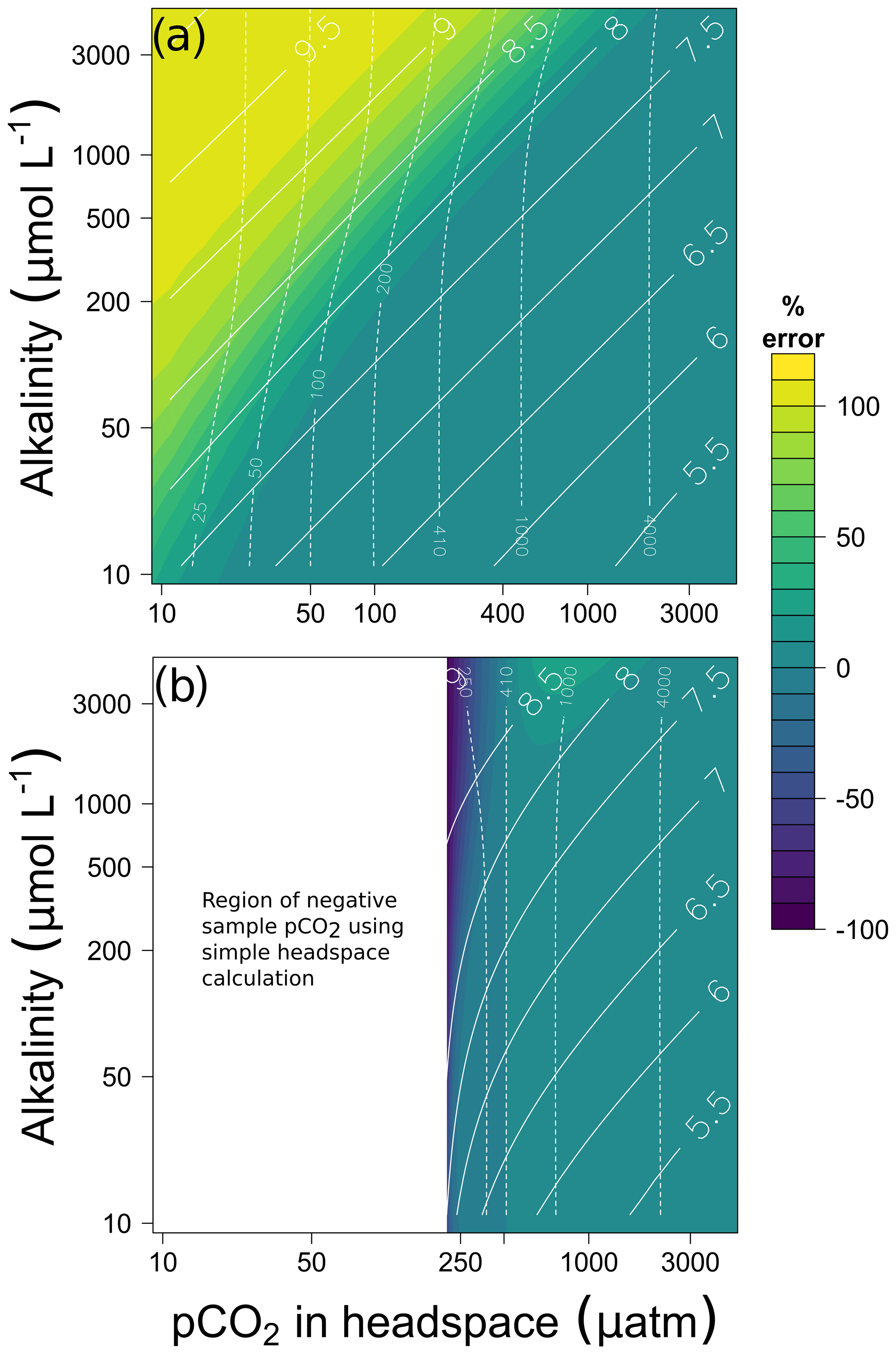
Figure 1 Error (%) when applying simple headspace calculations of pCO₂ on hypothetical water samples of different alkalinity and pCO₂ in the headspace after equilibration for (a) CO₂-free gas headspace and (b) ambient-air headspace assuming a pressure of 1 atm. The resulting pH and pCO₂ of the samples are depicted as full and dashed lines, respectively. The headspace ratio is 1 : 1, and the equilibration and field temperature is 20 ^∘C. Note the log scale in all axes. In panel (b) results for pCO₂ in headspace after equilibration lower than 215 µatm are masked, because they would imply negative pCO₂ in the sample.

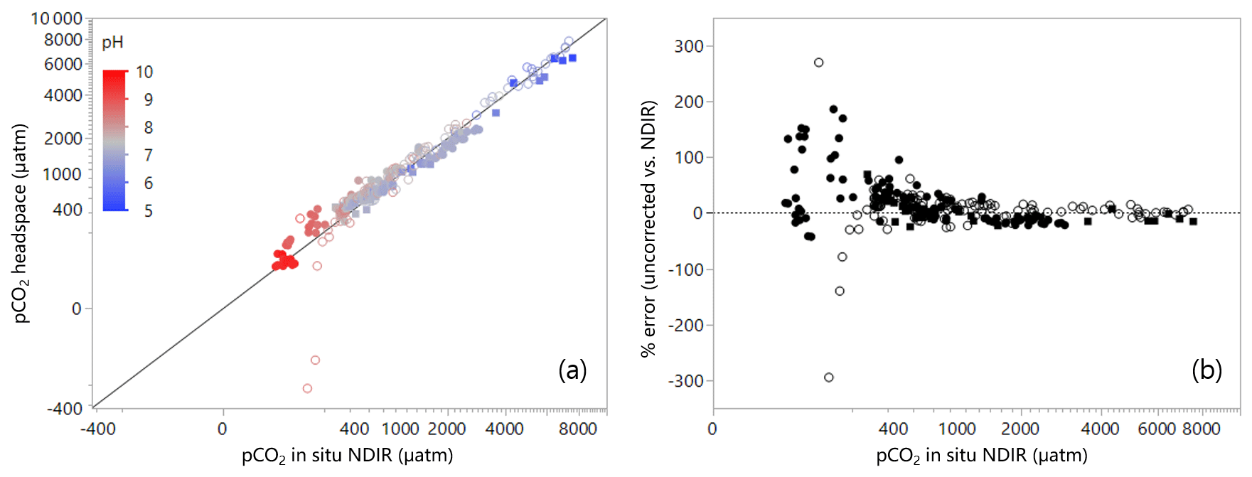
Figure 2 (a) Field data from 11 lakes, five reservoirs, and three streams in Germany, Canada, and Malaysia comparing pCO₂ derived from simple headspace analysis with direct pCO₂ measurements by NDIR analysis (pH colour coded). Note the cube-root scale in both axes. (b) Difference between the pCO₂ derived from the simple headspace analysis and the direct pCO₂ measurements by NDIR analysis expressed as error (%) as a function of the directly measured pCO₂ by NDIR analysis. Note the cube-root scale in the x axis. Open-circle symbols: ambient-air headspace; closed-circle symbols: CO₂-free gas headspace; and closed-square symbols: pre-measured-CO₂ gas (between 150 to 250 ppm) headspace applied.

Our field dataset is consistent with the theoretical predictions. While the fit between the simple headspace calculation and NDIR values over the whole range of values can be considered adequate overall (Fig. 2a, R²=0.92), it is clear that the deviations can become very large (up to about 300 %), particularly at water pCO₂ values < 600 µatm (Fig. 2b). As expected from the simulations, the error in undersaturated samples was positive when using CO₂-free gas as headspace and negative (sometimes impossible negative results) when using ambient air (Fig. 2b). The error became negligible at pCO₂ above 1000 µatm (Fig. 2b). Data scatter was considerable as was observed previously (Johnson et al., 2010), most probably because the analytical error of the applied methods was often in the same range as the absolute difference between both methods.

3.2 Error magnitude depends on the experimental procedure

The maximum error depends on how much CO₂ is exchanged between water and headspace. The more gas is exchanged between water and headspace the higher the error is. Thus, the error increases with decreasing solubility coefficient or HR. In high-alkalinity samples, the error can be significantly reduced by using a smaller headspace-to-water ratio (Fig. 3). By lowering the headspace ratio from 1 to 0.2 at 20 ^∘C, the error can be reduced from about 50 % to about 10 %.

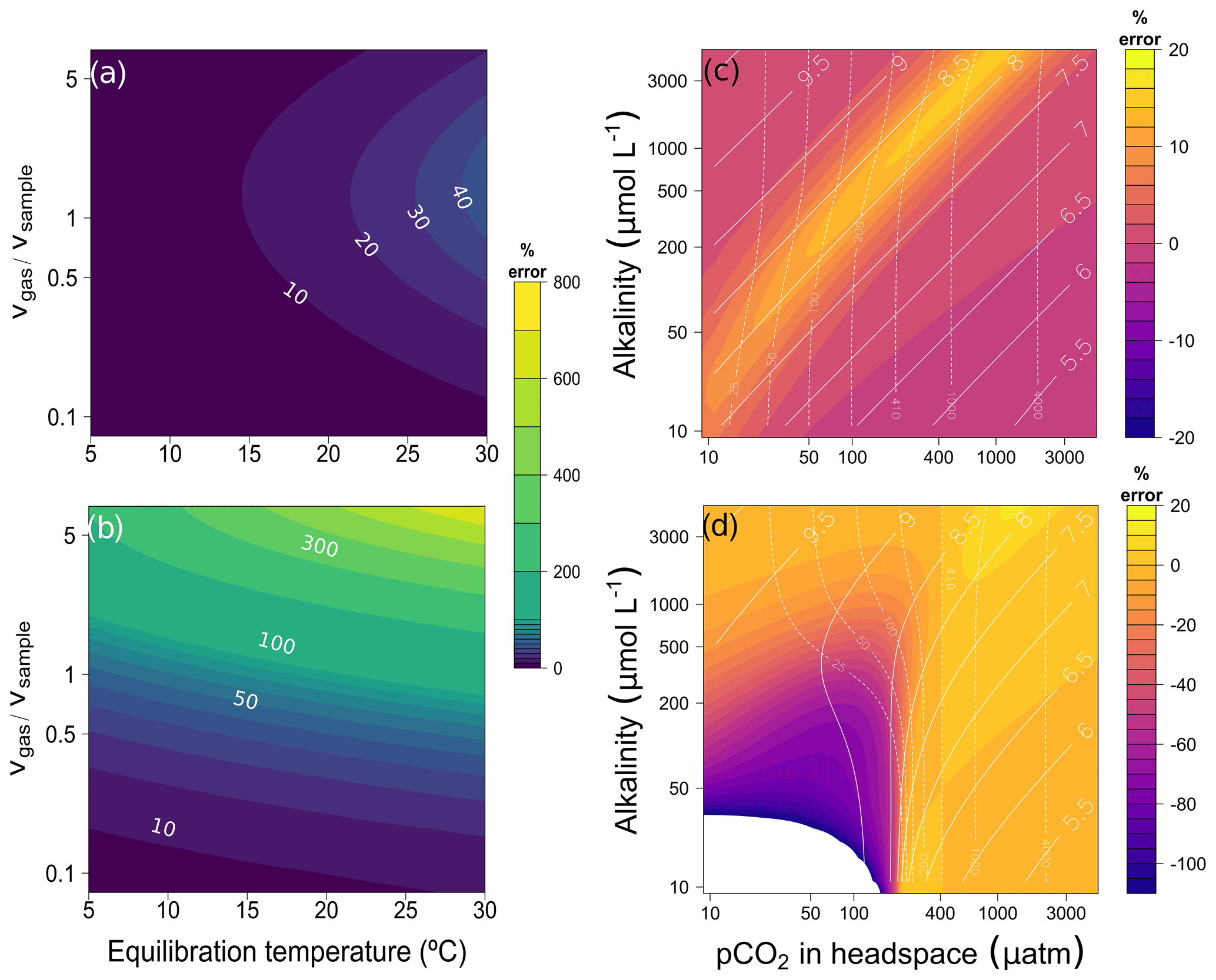
Figure 3 Error (%) when applying simple headspace calculation depending on headspace ratio and equilibration temperature for (a) 100 µmol L⁻¹ and (b) 1000 µmol L⁻¹ alkalinity. Panels (a) and (b) were constructed using highly undersaturated conditions (headspace pCO₂ = 50 µatm after equilibration and field water temperature of 20 ^∘C). The values of some isolines are added for reference. (c) Error (%) applying our complete headspace method when the alkalinity value supplied for calculations is off the real alkalinity of the sample by +50 %. The results are for hypothetical water samples of different alkalinity and pCO₂ in the headspace after equilibration using CO₂-free gas headspace, a headspace ratio of 1 : 1, and an equilibration and field temperature of 20 ^∘C. (d) Like panel (c) but with air headspace. All calculations assume a pressure of 1 atm.

Since solubility of CO₂ depends on temperature, the equilibration temperature also affects headspace equilibration. Due to lower solubility at higher temperature, more gas evades into the headspace, and thus the error increases with increasing temperature (Fig. 3a, b). At a HR of 1, the error increases from 97 % at 20 ^∘C to 111 % at 25 ^∘C in a high (1 mmol L⁻¹) alkalinity sample. Thus, the error can be significantly reduced by lowering the equilibration temperature. A possible way to take advantage of this is to perform headspace equilibration at in situ temperature in the field, as has been done in several studies. If in situ water temperature is lower than typical laboratory temperature, the error is thereby reduced. However, care must be taken to make sure that the exact equilibration temperature is known. For example, an error of 1 ^∘C in the equilibration temperature results in a 2 % different pCO₂ value (TA = 1 mmol L⁻¹, pCO₂ = 1000 µatm, HR = 1) (Fig. A1a). Both ambient air and N₂ can be used as headspace gas. Using N₂, however, eliminates the error associated with the exact quantification of pCO_2 Before. Using the same example, an unlikely error of 100 ppm in the headspace gas (mCO_{2 Before eq}) results in a 6.4 % different pCO₂ result (Fig. A1b).

3.3 What about kinetics?

CO₂ reactivity with water would not cause a problem for headspace analysis if the reaction kinetics were slow compared to physical headspace equilibration. The slowest reaction of the carbonate system is the hydration of CO₂, which has a first-order rate constant of 0.037 s⁻¹ (Soli and Byrne, 2002), so that chemical equilibration of CO₂ in water is in the range of seconds (Zeebe and Wolf-Gladrow, 2001; Schulz et al., 2006). This means that chemical equilibrium reactions are faster than physical headspace equilibration, and the chemical system can be assumed to always be in equilibrium. Thus, the reactions of the carbonate system have to be fully considered in headspace analysis of CO₂.

3.4 Correction of CO₂ headspace data

If other information regarding the carbonate system of the sample is known (alkalinity or DIC), one can correct for the bias induced by simple headspace calculations. A procedure to correct headspace CO₂ data using pH and alkalinity is already available in the standard operating procedure (SOP) no. 4 in Dickson et al. (2007) for marine samples and could be adapted to freshwater samples as well. For convenience, we provide here a modified procedure when the alkalinity of the sample is known by introducing an analytical solution to the equilibrium problem (iterative in SOP no. 4) and by using dissociation constants that may be more appropriate to fresh waters. The procedure essentially involves estimating the exact pH of the equilibrium solution before and after equilibration. If the alkalinity of the sample is known, the pH (−log ₁₀[H⁺]) of the aqueous solution after equilibration can be obtained by finding the roots of the third-order polynomial:

$$\begin{array}{}\text{(2)}& \begin{array}{rl}\mathrm{0}& =[{\mathrm{H}}^{+}{]}^{\mathrm{3}}+\mathrm{TA}\cdot [{\mathrm{H}}^{+}{]}^{\mathrm{2}}-\left(\left[{\mathrm{CO}}_{\mathrm{2}}\right]K_{\mathrm{1}}+K_{\mathrm{w}}\right)\left[{\mathrm{H}}^{+}\right]\\ & -\mathrm{2}{K}_{\mathrm{1}}{K}_{\mathrm{2}}\left[{\mathrm{CO}}_{\mathrm{2}}\right],\end{array}\end{array}$$

where $\left[{\mathrm{CO}}_{\mathrm{2}}\right]=p{\mathrm{CO}}_{\mathrm{2}}\cdot K_{\mathrm{h}\mathrm{Eq}}$ and from which one can obtain the ionization fraction for CO₂ (${\mathit{\alpha }}_{{\mathrm{CO}}_{\mathrm{2}}}$) as

$$\begin{array}{}\text{(3)}& {\propto }_{{\mathrm{CO}}_{\mathrm{2}}}={\displaystyle \frac{\mathrm{1}}{\mathrm{1}+\frac{K_{\mathrm{1}}}{\left[{\mathrm{H}}^{+}\right]}+\frac{K_{\mathrm{1}}{K}_{\mathrm{2}}}{[{\mathrm{H}}^{+}{]}^{\mathrm{2}}}}},\end{array}$$

where K₁ and K₂ are the temperature-dependent equilibrium constants for the dissociation reactions for bicarbonates and carbonates, respectively (Millero, 1979), and for estuarine conditions (Millero, 2010), as amended in Orr et al. (2015). K_w is the dissociation constant of water into H⁺ and OH⁻ (Dickson and Riley, 1979). The total DIC contained in the original sample (DIC_orig) can then be calculated as

$$\begin{array}{}\text{(4)}& {\mathrm{DIC}}_{\mathrm{orig}}={\displaystyle \frac{{\mathrm{CO}}_{\mathrm{2}}}{{\mathit{\alpha }}_{{\mathrm{CO}}_{\mathrm{2}}}}}+\left({\mathrm{CO}}_{\mathrm{2}\mathrm{HS}\mathrm{after}}-{\mathrm{CO}}_{\mathrm{2}\mathrm{HS}\mathrm{before}}\right),\end{array}$$

where CO₂ is the amount of CO₂ in the equilibrated water (mol), and CO_{2 HS after} and CO_{2 HS before} are the amount of CO₂ in the headspace after and before equilibration (mol). Given the DIC concentration of the original solution from Eq. (4) ([DIC] = DIC${}_{\mathrm{orig}}/V_{\mathrm{liquid}}$), the pH of this solution prior to equilibration can be obtained by finding the roots of the fourth-order polynomial,

$$\begin{array}{}\text{(5)}& \begin{array}{rl}\mathrm{0}& =[{\mathrm{H}}^{+}{]}^{\mathrm{4}}+\left(\mathrm{TA}+K_{\mathrm{1}}\right)\cdot [{\mathrm{H}}^{+}{]}^{\mathrm{3}}\\ & +\left(\mathrm{TA}\cdot K_{\mathrm{1}}-K_{\mathrm{w}}+K_{\mathrm{1}}{K}_{\mathrm{2}}-{\left[\mathrm{DIC}\right]}_{\mathrm{orig}}{K}_{\mathrm{1}}\right)\cdot {\left[{\mathrm{H}}^{+}\right]}^{\mathrm{2}}\\ & +\left(K_{\mathrm{1}}{K}_{\mathrm{2}}\cdot \mathrm{TA}-K_{\mathrm{1}}{K}_{\mathrm{w}}-\mathrm{2}{\left[\mathrm{DIC}\right]}_{\mathrm{orig}}{K}_{\mathrm{1}}{K}_{\mathrm{2}}\right)\cdot \left[{\mathrm{H}}^{+}\right]\\ & -K_{\mathrm{1}}{K}_{\mathrm{2}}{K}_{\mathrm{w}},\end{array}\end{array}$$

to then estimate the corresponding ionization fraction ${\mathit{\alpha }}_{{\mathrm{CO}}_{\mathrm{2}}}^{\prime }$ as in Eq. (3) above and calculate the original pCO₂ of the sample as

$$\begin{array}{}\text{(6)}& p{\mathrm{CO}}_{\mathrm{2}}={\displaystyle \frac{{\mathit{\alpha }}_{{\mathrm{CO}}_{\mathrm{2}}}^{\prime }\cdot {\left[\mathrm{DIC}\right]}_{\mathrm{orig}}}{K_{\mathrm{h}\mathrm{Sample}}}},\end{array}$$

where K_h Sample is determined for the water temperature during field sample collection (for simplicity, the equations above assume 1 atm pressure). We applied the above correction procedure to our samples, where pCO₂ was measured in several samples using both headspace and in situ NDIR methods together with measured alkalinity data. Figure 4 shows that the corrected values matched the in situ NDIR values nearly perfectly (r²=0.98), whereas the simple headspace calculations resulted, as expected, in significant underestimation for undersaturated conditions, particularly for samples equilibrated with ambient air.

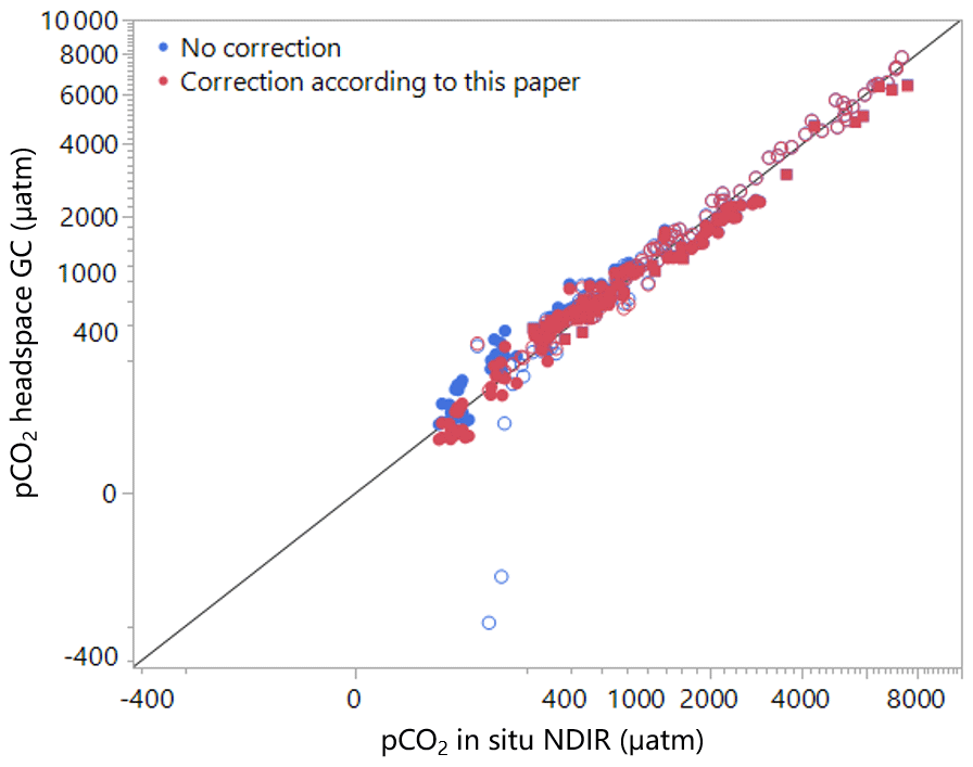
Figure 4 Comparison of uncorrected and corrected data with direct pCO₂ measurements by NDIR analysis. Note the cube-root scale in both axes. Open-circle symbols: ambient-air headspace; closed-circle symbols: CO₂-free gas headspace; and closed-square symbols: pre-measured-CO₂ gas (between 150 to 250 ppm) headspace applied.

We examined the sensitivity of the correction procedure to the precision of the alkalinity measurements and found that the error associated with alkalinity determination does not severely impact the final pCO₂ estimate when using N₂ as a headspace gas. For example, the error in the corrected pCO₂ values is always below 20 % even when the alkalinity is known only to within 50 % error (Fig. 3c). However, more precise alkalinity values are required when using ambient air as a headspace gas in undersaturated conditions (Fig. 3d).

Lastly, our simulations (Figs. 2 and 4) provide a complete analysis of the effects of the environmental and methodological conditions on the error incurred when using the simple headspace technique for estimating pCO₂. However, they do not assess how often such problematic conditions occur in inland water systems. To address this question, we applied our correction procedure to a dataset from 377 Canadian lakes (Huot et al., 2019). These results show a significant deviation between corrected and uncorrected values, particularly in lakes with high alkalinity (> 900 µmol L⁻¹, Fig. B1b), and ignoring the correction would have resulted in errors > 20 % in about 47 % of the data. Furthermore, our analysis illustrates how a larger headspace ratio significantly exacerbates the magnitude of the error (Fig. B1b).

The correction calculations have been implemented in an R script and, for a user-friendly interface, as a JMP add-in (or JSL script) (https://github.com/icra/headspace, last access: 3 March 2021). Roots of the polynomials (Eqs. 2 and 5) can be solved using either standard analytical formulas or by iterative algorithms. For the analytical solution, our script uses a combined form of the computational steps described in Zwillinger (2018) for both the cubic and quartic polynomials to find their first real roots. Analytical solutions are faster than iterative algorithms but can suffer small numerical instabilities (SD ≈ 1 ppm) in extreme situations (alkalinity > 4000 µmol L⁻¹ and pCO₂ < 100 ppm) due to limitations inherent to double-precision numerical calculations. The provided scripts consider the barometric pressure and thus allow calculation of pCO₂ as well as CO₂ concentration (µmol L⁻¹) for in situ conditions.

4 Conclusions

The headspace method has been used in several studies about CO₂ fluxes from surface waters. Our error analysis shows that the usual headspace method can be used (error < 5 %) if the pH is below 7.5 or pCO₂ is above 1000 µatm (TA < 900 µmol L⁻¹, air headspace), a typical situation in most boreal systems. However, the standard headspace method introduces large errors and cannot be used reliably for undersaturated samples, which are typical of eutrophic or low-DOC systems. In all other cases, not accounting for the chemical equilibrium shift leads to a systematic overestimation. The magnitude of the error can be reduced by increasing the water–headspace ratio or lowering the equilibration temperature. The magnitude of that error can be roughly estimated from Fig. 1. If alkalinity is known, pCO₂ obtained from headspace equilibration can be corrected by the provided scripts. We therefore recommend to always measure alkalinity if the headspace method is to be used for pCO₂ determinations. The procedure can also be used to correct historical pCO₂ data. Our field data showed that the correction works well even in highly undersaturated conditions and is not very sensitive to the precise determination of alkalinity if N₂ is used as a headspace gas. The precision of the corrected pCO₂ is similar to that obtained from direct pCO₂ measurement using a field NDIR analyser coupled to an online equilibrator (Cole and Prairie, 2009; Yoon et al., 2016).

Appendix A: Sensitivity analysis equilibration temperature and CO_2 Beforeeq

Figure A1 Error for a hypothetical sample with CO_{2 Before eq} = 400 ppm, CO_{2 after eq} = 1000 ppm, equilibration temperature of 20 ^∘C, and HR = 1 (a) depending on error in equilibration temperature and (b) depending on error in initial headspace gas composition.

Appendix B: Application of our correction to a large Canadian dataset

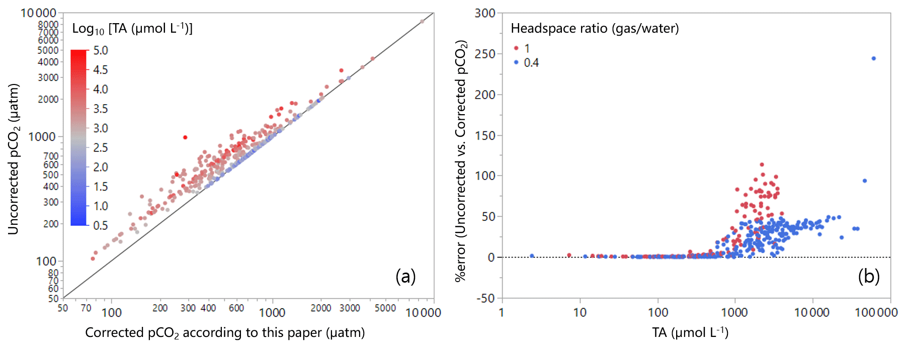
Figure B1 Field data from 377 lakes across Canada (a) for comparing pCO₂ derived from simple headspace calculation with that from the corrected headspace calculation according to this paper (Log₁₀ [TA (µmol L⁻¹)] colour coded). (b) Difference between the uncorrected and corrected pCO₂ expressed as error (%) as a function of TA (µmol L⁻¹) (the headspace ratio colour coded). Note that CO₂-free gas was used for headspace, and TA values were derived from DIC measurement and pH. More information about the dataset can be found in Huot et al. (2019).