Climate change and elevated CO₂ favor forest over savanna under different future scenarios in South Asia

South Asian vegetation provides essential ecosystem services to the 1.7 billion inhabitants living in the region. However, biodiversity and ecosystem services are threatened by climate and land-use change. Understanding and assessing how ecosystems respond to simultaneous increases in atmospheric CO₂ and future climate change is of vital importance to avoid undesired ecosystem change. Failed reaction to increasing CO₂ and climate change will likely have severe consequences for biodiversity and humankind. Here, we used the adaptive dynamic global vegetation model version 2 (aDGVM2) to simulate vegetation dynamics in South Asia under RCP4.5 and RCP8.5, and we explored how the presence or absence of CO₂ fertilization influences vegetation responses to climate change. Simulated vegetation under both representative concentration pathways (RCPs) without CO₂ fertilization effects showed a decrease in tree dominance and biomass, whereas simulations with CO₂ fertilization showed an increase in biomass, canopy cover, and tree height and a decrease in biome-specific evapotranspiration by the end of the 21st century. The predicted changes in aboveground biomass and canopy cover triggered transition towards tree-dominated biomes. We found that savanna regions are at high risk of woody encroachment and transitioning into forest. We also found transitions of deciduous forest to evergreen forest in the mountain regions. Vegetation types using C₃ photosynthetic pathway were not saturated at current CO₂ concentrations, and the model simulated a strong CO₂ fertilization effect with the rising CO₂. Hence, vegetation in the region has the potential to remain a carbon sink. Projections showed that the bioclimatic envelopes of biomes need adjustments to account for shifts caused by climate change and elevated CO₂. The results of our study help to understand the regional climate–vegetation interactions and can support the development of regional strategies to preserve ecosystem services and biodiversity under elevated CO₂ and climate change.

1 Introduction

Global climate has been identified as the primary determinant of large-scale natural vegetation patterns (Overpeck et al., 1990). Climate change has affected global vegetation pattern in the past and caused numerous shifts in plant species distribution over the last few decades (Chen et al., 2011; Thuiller et al., 2008). It is expected to have even more pronounced effects in the future and may lead to drastically increasing species extinction rates in various ecosystems (Brodie et al., 2014). Natural ecosystems have been and continue to be exposed to increased climate variability and abrupt changes caused by increased intensity and frequency of extreme events such as heat waves, drought and flooding (Herring et al., 2018). At the same time, they are under severe pressure due to anthropogenic disturbance and land conversion. Rising levels of atmospheric CO₂ are a strong driver of climate-induced vegetation changes (Allen et al., 2014). Anthropogenic CO₂ emissions account for approximately 66 % of the total anthropogenic greenhouse forcing (Forster et al., 2007) and are thus largely responsible for contemporary and future global climate change (Parry et al., 2007). Rising CO₂ is expected to alter distributions of plant species and ecosystems (Parry et al., 2007) both indirectly through its influence on global temperatures and precipitation patterns (Cao et al., 2010), two main drivers of vegetation dynamics, and directly via its physiological effects on plants (Nolan et al., 2018). It is therefore of vital importance to understand how ecosystems respond to simultaneous increases in atmospheric CO₂ and temperature, to changes in precipitation regime, and to altered ecosystem water balance in order to avoid critical ecosystem disruptions and the resulting consequences for biodiversity and humankind.

Increases in temperatures, decreases in precipitation and changes in precipitation seasonality can cause loss of vegetation biomass. Plants using C₃ photosynthetic pathway are often not saturated at the current atmospheric CO₂, whereas plants using the C₄ photosynthetic pathways are already at their physical optimum at current atmospheric CO₂ levels (Ehleringer and Cerling, 2002). The physiology of C₃ plants implies that elevated atmospheric CO₂ improves their ability for carbon uptake due to the CO₂ fertilization (Woodrow and Berry, 1988) and enhances carbon sequestration (Leakey et al., 2009; Norby and Zak, 2011) as well as plant water use efficiency (Soh et al., 2019). This has also been observed in long-term free-air carbon dioxide enrichment (FACE) experiments (Norby and Zak, 2011). Thus, elevated CO₂ influences photosynthesis and thereby affects other physiological processes such as respiration, decomposition (Doherty et al., 2010), evapotranspiration (ET) and biomass accumulation (Frank et al., 2015). Increasing CO₂ concentration has been associated with woody cover increase in structurally open tropical biomes such as grasslands and savannas (Stevens et al., 2017). This widespread proliferation of woody plants into arid and semiarid ecosystems has been attributed to increased water use efficiency in C₃ plants that facilitates woody sapling establishment and growth due to higher drought tolerance (Kgope et al., 2010; Stevens et al., 2017). These CO₂ effects on plant growth and competition can alter community structure (height distribution), ecosystem productivity, climatic niches of ecosystems and biome boundaries (Nolan et al., 2018; Wingfield, 2013). Change in vegetation distribution and altered vegetation structure feed back on climate by altering fluxes of energy, moisture, and CO₂ between land and atmosphere (Friedlingstein et al., 2006). Feedback mechanisms also involve vegetation‐mediated changes in albedo, surface roughness, land‐-atmosphere fluxes and evapotranspiration (Field et al., 2007; Richardson et al., 2013).

Enhanced plant growth due rising CO₂ implies rapid leaf area development and more total leaf area could translate into higher transpiration (Leakey et al., 2009). However, elevated CO₂ concentrations may decrease leaf stomatal conductance to water vapor, which could reduce transpiration. Evapotranspiration (ET) is a key ecophysiological process in the soil–vegetation–atmosphere continuum (Feng et al., 2017). Annually, 64 % of the total global land-based precipitation is returned to the atmosphere through ET (Zhang et al., 2016). Environmental change and concurrent vegetation changes alter ET and affect water availability (Mao et al., 2015), especially in arid and semiarid regions. In these regions, ET affects surface and subsurface processes such as cloud development, land surface temperature and groundwater recharge (Fisher et al., 2011).

South Asia is home to approximately 1.7 billion people and is one of the regions most vulnerable to climate change (Eckstein et al., 2018). It hosts four of the world's biodiversity hotspots (Myers et al., 2000) and harbors different biome types ranging from tropical in the south to temperate in the north at the fringe of the Himalayas. These hotspots are characterized by high levels of diversity and endemism, and they are threatened by climate change and anthropogenic land use (Deb et al., 2017). For instance, woody encroachment due to rising CO₂ threatens South Asian savannas (Kumar et al., 2020), and sifting cultivation in the northeastern part of South Asia threatens biodiversity (Bera et al., 2006).

Due to the absence of long-term field experiments such as FACE experiments, in the dominant biomes of the region, modeling studies are valuable tools to close existing knowledge gaps. Dynamic global vegetation models (DGVMs, Prentice et al., 2007) are particularly well suited to address questions that focus on vegetation response to changing environmental drivers, e.g., climate and CO₂. While most DGVM studies in South Asia focused on the vulnerability of forests to climate change (Chaturvedi et al., 2011; Ravindranath et al., 2006, 1997), they often overlooked the severely threatened savanna biome. These studies were further limited by the utilization of models with fixed ecophysiological parameters and traits, e.g., fixed carbon allocation values to assign carbon to plant biomass pools, fixed specific leaf area (SLA) and pre-defined bioclimatic limits that were derived from contemporary climatology in order to constrain the spatial distribution of plant functional types (PFTs). Moreover, many DGVMs used in these studies do not account for life history, eco-evolutionary processes and trait variability among individual plants (Kumar and Scheiter, 2019). While some global-scale studies have investigated the potential effect of increasing CO₂ on natural vegetation, carbon sequestration and biome boundaries (e.g., Hickler et al., 2006; Sato et al., 2007; Smith et al., 2014), detailed modeling studies focusing explicitly on different biomes in South Asia have not been conducted. The physiological effects of increased CO₂ and climate change on South Asian vegetation are uncertain and need to be addressed in order to improve understanding of regional ecosystem functioning as well as implications for biodiversity conservation.

To address the knowledge gaps in existing studies, we used the aDGVM2 (adaptive dynamic global vegetation model version 2), an individual- and trait-based vegetation model that combines elements of traditional DGVMs (Prentice et al., 2007) with newly implemented approaches for selection and trait filtering. In aDGVM2, environmental conditions select for the plants with trait value combinations that make them successful under these conditions. Therefore, plant communities that are adapted to site-specific environmental conditions dynamically assemble and emerge as a reaction to the environmental forcing (Langan et al., 2017; Scheiter et al., 2013). Originally, aDGVM2 had been tested for Amazonia (Langan et al., 2017) and Africa (Gaillard et al., 2018; Pfeiffer et al., 2019). In order to adapt it to South Asian ecosystems and their diversity, we included C₃ grasses, improved ecophysiological processes such as the leaf energy budget in order to estimate leaf temperature, implemented separate temperature sensitivities for C₃ and C₄ photosynthetic capacity (V_cmax), and included snow in the water balance model.

In this study we used the updated version of aDGVM2 and addressed the following questions:

1. How do projected changes in climate and CO₂ following two representative concentration pathways (RCP8.5 and RCP4.5, Meinshausen et al., 2011) change the distribution, boundaries and climatic niches of biomes in South Asia?

2. How does the relationship between projected biomass, ET, temperature and precipitation change in response to CO₂ fertilization?

3. What is the sensitivity of predicted changes in relation to presence and absence of CO₂ fertilization?

Based on our results we analyzed climate–vegetation interactions to improve our understanding of how to manage and mitigate impacts on biomes under climate change and increasing CO₂.

2 Methods

2.1 Description of the study region

Approximately 1.7 billion people populate South Asia, i.e., the Indian subcontinent, Afghanistan and Myanmar. South Asia incorporates a wide range of bioclimatic zones with distinctive biomes, ecosystem types and species (Rodgers and Panwar, 1988). Climatic conditions are controlled by interactions between the South Asian summer monsoon system and the region's complex topography. The climatic envelope ranges from tropical arid and semiarid regions in the west to humid tropical regions supporting rain forests in the northeast and temperate vegetation at the fringe of the Himalayas. Excluding the Himalayan regions, South Asia has a mean annual temperature of approximately 24 ^∘C with very low spatial variability. Mean annual precipitation (MAP) is 1190 mm, ranging from less than 500 mm in the warm desert zone in the west to more than 3500 mm in the northeast. The steep elevation gradients ranging from sea level to 8800 m result in a rich diversity of ecosystems that can alternate in areas of a few hundred square kilometers. Topography is recognized as a strong driver of ecological patterns, for example those related to forest structure and composition, floristic diversity and soil fertility (Gallardo-Cruz et al., 2009; Jucker et al., 2018; Sinha et al., 2018). South Asia hosts four major global biodiversity hotspots, namely the Western Ghats, Himalayas, India and Myanmar, and Sri Lanka (Myers et al., 2000). These hotspots include a wide diversity of ecosystems such as mixed wet evergreen, dry evergreen, deciduous and montane forests. Further vegetation types are alluvial grasslands and subtropical broadleaf forests along the foothills of the Himalayas, temperate broadleaf forests in the mid-hills, mixed conifer and conifer forests in the higher hills, savanna in the Deccan region and southern part of Malaysia, and alpine meadows above the tree line.

2.2 Model description

For this study we used aDGVM2 (Scheiter et al., 2013; Langan et al., 2017; Gaillard et al., 2018), a DGVM with a dynamic trait approach. In the Supplement we summarize main features of aDGVM2 and explain how the physiological effects of changing CO₂ concentration and rising temperature are simulated in a process-based way in the aDGVM2 by the implemented photosynthesis routine. To adapt the aDGVM2 to the requirements of the study region, we incorporated new subroutines into the model. We improved the representation of (a) the water balance by including snow, (b) the carboxylation rate, and (c) leaf temperature, and (d) we included C₃ grasses (previous model versions only simulated C₄ grasses).

• a.

  Water balance.

  In aDGVM2, the soil water module is based on the tipping-bucket concept. As the model was originally developed with a strong focus on tropical and subtropical forest and savanna regions, the original model version only considered water input in the form of rain (see Langan et al., 2017). In the updated model version, precipitation is assigned as snow when daily mean air temperature drops below 0 ^∘C. Snow accumulates on the soil surface or is added on top of an existing snowpack. The snowpack persists as long as air temperature remains below 0 ^∘C. Once temperature rises above 0 ^∘C, water from snowmelt is added to the soil water pool and becomes available to plants. This process may improve the water availability for plants at the beginning of spring, for example in the Himalayan region. Snowmelt (S_melt, mm/day) is calculated following Choudhury et al. (1998) as

  $$\begin{array}{}\text{(1)}& S_{\mathrm{melt}}=\mathrm{1.5}+K_{\mathrm{m}}{P}_{\mathrm{precip}}(T_{\mathrm{a}}-T_{\mathrm{snow}})S_{\mathrm{pack}},\end{array}$$

  where K_m is the coefficient of snowmelt (0.007 mm/day/^∘C), S_pack is the depth of the snowpack (mm) and is equivalent to the accumulated solid portion of precipitation, T_a is the daily mean air temperature (^∘C), P_precip is precipitation (mm/day), and T_snow is the maximum temperature where precipitation falls as snow (0 ^∘C). We do not consider insulation effects of the snowpack in the model.

• b.

  Carboxylation rate.

  In earlier versions of aDGVM2, leaf-level photosynthesis was calculated at the population level; i.e., it was assumed that all plants of a simulated vegetation stand have the same leaf-level photosynthetic rate. Only C₃- and C₄-type photosynthesis were distinguished. We therefore implemented new routines to calculate photosynthesis at a daily time step for each individual plant. We further incorporated an empirical relation between specific leaf area (A_SLA, mm²/mg) and leaf nitrogen content per unit area (N_a, g/m²) following Sakschewski et al. (2015):

  $$\begin{array}{}\text{(2)}& N_{\mathrm{a}}=\mathrm{6.89}{A}_{\mathrm{SLA}}^{-\mathrm{0.571}}.\end{array}$$

  The standard maximum carboxylation rate of rubisco per leaf area (V_cmax,25, µmol/m²/s) was derived from the TRY database (Kattge and Knorr, 2007) by Sakschewski et al. (2015) and is calculated as

  $$\begin{array}{}\text{(3)}& V_{\mathrm{cmax},\mathrm{25}}=\mathrm{31.62}{N}_{\mathrm{a}}^{\mathrm{0.501}},\end{array}$$

  where V_cmax,25 is V_cmax at 25 ^∘C. In the model, A_SLA is linked to the matric potential at 50 % loss of xylem conductance (P50; see Langan et al., 2017). The trade-off between A_SLA and V_cmax mediated by leaf traits (N_a) introduces variability in the spectrum of tree growth strategies in aDGVM2. A_SLA is linked to leaf longevity (LL) in aDGVM2, such that it affects the leaf turnover rates (represented by Eq. 72, in Appendix, Langan et al., 2017). Leaves with high A_SLA have shorter LL and higher turnover rates than leaves with low A_SLA (and vice versa). The correlation between A_SLA, P50 and LL represents the trade-off between two opposing resource strategies, i.e., conservation vs. rapid acquisition of soil water and nutrients (Wright et al., 2005). Trees that invest more carbon into their leaves (low A_SLA) enhance their structural stability but have lower leaf turnover to mitigate the higher initial carbon investment.

  The effect of temperature on photosynthesis is well described (Kirschbaum, 2004), and temperature may influence photosynthesis both directly, via temperature dependency of enzyme-mediated metabolic rates of carboxylation and the Calvin cycle (Sharkey et al., 2007), and indirectly, via its effect on transpiration and plant water uptake and transport (Urban et al., 2017). The maximum carboxylation rate (V_cmax) increases with temperature until it reaches an optimum, and it decreases again at temperatures above the optimum (Kattge and Knorr, 2007) due to reductions in enzyme activity. Above 30 ^∘C the electron transport chain is gradually inhibited, and at temperatures above 40 ^∘C the denaturation of rubisco and associated proteins becomes relevant (Lloyd et al., 2008). The temperature dependency of the carboxylation rate (V_cmax) is expressed as

  $$\begin{array}{}\text{(4)}& V_{\mathrm{cmax}}={\displaystyle \frac{V_{\mathrm{cmax},\mathrm{25}}{\mathrm{2}}^{\mathrm{0.1}(T_{\mathrm{leaf}}-\mathrm{25})}}{(\mathrm{1}+e^{\mathrm{0.3}(T_{\mathrm{low}}-T_{\mathrm{leaf}})})(\mathrm{1}+e^{\mathrm{0.3}(T_{\mathrm{leaf}}-T_{\mathrm{upp}})})}},\end{array}$$

  where T_leaf is the leaf temperature in ^∘C (see next paragraph for calculation). The photosynthetic model of Collatz et al. (1992) and Collatz et al. (1992) assumes specific values of T_upp and T_low for C₃ and C₄ plants, respectively (Tables S1 and S2 in the Supplement). These temperature ranges from −10 to 36 ^∘C and from 13 to 45 ^∘C for C₃ and C₄ photosynthetic pathways, respectively, allow plants to grow most efficiently in their plant-specific climatic niches.

• c.

  Leaf temperature.

  We calculate leaf temperature following the leaf-level energy budget concept (Gates, 1968). Leaf-level photosynthesis, activity of leaf enzymes and transpiration depend on leaf temperature (T_leaf, ^∘C), calculated as

  $$\begin{array}{}\text{(5)}& T_{\mathrm{leaf}}=T_{\mathrm{air}}+\left({\displaystyle \frac{R_{\mathrm{n}}-\mathit{\lambda }E{r}_{\mathrm{gb}}}{\mathit{\rho }{C}_P}}\right),\end{array}$$

  where T_air is air temperature (^∘C), R_n is net radiation absorbed by the leaf (MJ/m²/day), λ is latent heat of vaporization (MJ/kg), E is evapotranspiration (m/day), r_gb is the boundary layer resistance (m/s), ρ is the air density (kg/m³) derived from atmospheric pressure (101.325 kPa at sea level) that is scaled according to the elevation and T_air, and C_P is the specific heat of dry air (MJ/kg/^∘C). Leaf temperature is used to calculate the temperature dependence of V_cmax used in the photosynthesis model routines in Eq. (4). Absorbed net radiation (R_n), r_gb and E are model state variables calculated from climate input used in aDGVM2 (T_air, long-wave and shortwave radiation, and ρ). The values of latent heat of vaporization (λ) and C_P are 2.45 MJ/kg and 2.71 MJ/kg/^∘C, respectively, and are assumed to be constant parameters in this model version.

• d.

  C₃ grasses.

  C₃ grasses were not included in previous aDGVM2 versions (Gaillard et al., 2018; Langan et al., 2017; Pfeiffer et al., 2019; Scheiter et al., 2013). We therefore implemented C₃ grasses, following the approach used for C₄ grasses in previous model versions, but adjusted the photosynthetic pathway (see Appendix S2 in Langan et al., 2017). C₃ and C₄ grasses use a different leaf-level photosynthesis model (Farquhar et al., 1980) following the implementations of Collatz et al. (1991, 1992). The optimum temperature ranges for carboxylation for C₃ and C₄ grasses are also different (Table S1). As C₃ grasses have higher cold tolerance than C₄ grasses (Liu and Osborne, 2008), we implemented frost intolerance for C₄ grasses but not for C₃ grasses. Frost is assumed to damage the tissue of C₄ grasses, and in aDGVM2 we kill 10 % of the living leaf biomass of C₄ grasses per frost day independent of frost severity.

2.3 Model forcing data

2.3.1 Climate data

We used GFDL-ESM2M climate data for the period 1950 to 2099 from the Inter-Sectoral Impact Model Inter-comparison Project (ISIMIP2), as historical climate simulated by GFDL-ESM2M showed satisfactory performance for South Asia (McSweeney and Jones, 2016). The general circulation model (GCM) output was bias-corrected in the Inter-Sectoral Impact Model Intercomparison Project (ISIMIP) and downscaled to a spatial resolution of 0.5^∘ × 0.5^∘ (Warszawski et al., 2014). We used average, maximum and minimum air temperatures, precipitation, surface downwelling shortwave radiation and long-wave radiation, near-surface wind speed, and relative humidity at a daily temporal resolution. We used two representative concentration pathways, namely RCP4.5 and RCP8.5 (Meinshausen et al., 2011). These scenarios assume increases in radiative forcing of 4.5 and 8.5 W/m² by 2100 (Van Vuuren et al., 2011) and increases in atmospheric CO₂ concentrations to 560 and 970 ppm by 2100, respectively (Van Vuuren et al., 2011).

2.3.2 Projected changes in temperature and precipitation

Mean annual precipitation (MAP) from GFDL-ESM2M does not show a clear trend when averaged for South Asia under RCP4.5 and RCP8.5, due to high inter-annual variability of precipitation (Fig. S1 in the Supplement). Yet, there are region-specific differences in precipitation change. The Western Ghats which are located between 73–77^∘ E and 8–21^∘ N and the eastern Himalayan region are projected to become wetter under both RCP4.5 and RCP8.5, whereas the western part of the region is projected to become drier by the end of the century under both RCPs (Fig. S2). MAP is projected to increase by more than 600 mm in the eastern Himalayas and Western Ghats but predicted to decrease by 400–600 mm in the western and central area of the region (Fig. S2). By the end of the 21st century, the mean annual temperature (MAT) of South Asia is expected to increase between ca. 1 and 3.5 ^∘C under RCP4.5 and between 1 and 6 ^∘C under RCP8.5, relative to the average temperature in the baseline period of 2000–2009 (Figs. S1 and S2). The western parts of the region and the Himalayan mountains are projected to experience higher increases in temperature than the rest of the region (Fig. S2).

2.3.3 Soil and elevation data

Soil data were obtained from FAO (http://www.fao.org/soils-portal, last access: March 2016,  Nachtergaele et al., 2009) and include information on soil properties and types. The soil properties include parameters required by aDGVM2: volumetric water-holding capacity, soil hydraulic conductivity, soil bulk density, soil depth, soil texture, soil carbon content, soil wilting point and field capacity (for details see Fig. S3b and Langan et al., 2017). A digital elevation model (DEM) at 90 m spatial resolution was obtained from the Shuttle Radar Topography Mission (SRTM, Fig. S3a http://srtm.csi.cgiar.org, last access: March 2016,  Jarvis et al., 2008). It was resampled to a spatial resolution of 0.5^∘ × 0.5^∘ to match the spatial resolution of climate data. In the model, elevation is used to calculate the surface pressure at a given altitude, which is used to scale up air density and partial pressure of oxygen. The partial pressure of oxygen is used to estimate the CO₂ compensation point of photosynthesis (Eq. 2 of Appendix S2 in Langan et al., 2017). We did not use slope and aspect in the model.

2.4 Model simulation protocol

To understand how climate and CO₂ fertilization interact to influence the future vegetation state in South Asia, we simulated all combinations of two climate scenarios (RCP4.5 and RCP8.5) and two CO₂ scenarios (CO₂ fertilization enabled or disabled, four scenarios in total). We simulated potential natural vegetation between 1950 and 2099 using daily climate data for RCP4.5 and RCP8.5 (see Sect. 2.3.1). For both scenarios, simulations were run with a CO₂ increase in line with RCP4.5 (hereafter RCP4.5+eCO₂) and RCP8.5 (hereafter RCP8.5+eCO₂) and with the same climate data but fixed CO₂ after 2005 at 375 ppm for RCP4.5 (hereafter RCP4.5+fCO₂) and RCP8.5 (hereafter RCP8.5+fCO₂). Fixing the CO₂ concentration after 2005 mimics a situation where CO₂ fertilization would not occur and vegetation only responds to the climate signal. All simulations were conducted with natural fire as implemented in aDGVM2 and at 0.5^∘ × 0.5^∘ spatial resolution. The aDGVM2 simulates 1 ha stands that are assumed to be representative for the vegetation at a larger scale; i.e., we assume that the stand-level vegetation homogeneously covers the grid cell. The “representative hectare approach” is a concession to computational limitation, as photosynthesis and physiological processes are simulated individually for all individual plants of a stand (up to 36 000 individuals). It balances adequate representation of trait diversity among individuals against computational constraints. Also due to computational constraints, we did not conduct replicate simulations.

To ensure that simulated vegetation had sufficient time to adapt to prevailing environmental conditions, we conducted simulations for 650 years, split into a 500-year spin-up phase and a 150-year transient phase. For the spin-up phase, we randomly sampled years of the first 30 years of daily climate data (1950 to 1979). For the transient phase, we used the sequence of daily climate data between 1950 and 2099. Trial simulations showed that a 500-year spin-up period is sufficient to ensure that vegetation is in a dynamic equilibrium state with environmental drivers.

2.5 Model benchmarking and evaluation

For benchmarking of aDGVM2 simulation results, we used five different remote sensing products: aboveground biomass (t/ha, Saatchi et al., 2011), tree height (m, Simard et al., 2011), tree cover (percent, Friedl et al., 2010), MODIS evapotranspiration (mm/year, Zhang et al., 2010) and natural vegetation type (Ramankutty et al., 2010). We used a 10-year average of MODIS ET and compared it to a 10-year average of model-simulated ET (mm/year; 2000–2009). All remote sensing data sets were aggregated to a 0.5^∘ × 0.5^∘ spatial resolution to match the spatial resolution of model simulations by calculating the mean of all values within each 0.5^∘ grid cell or using nearest-neighbor aggregation in the case of vegetation type (“raster” package in R, Hijmans and van Etten, 2012). We first compared model results and observations assuming that the entire study region is covered by natural vegetation (Fig. 1). Then we repeated the comparisons only for areas with predominantly natural cover; i.e., we masked out areas with more than 50 % managed land (Fig. S4, land cover classes 7 “Cultivated and Managed Vegetation” and 9 “Urban and Built-up” in  Tuanmu and Jetz, 2014). We calculated the normalized mean squared error (NMSE) and coefficient of determination (R²) to quantify agreement between data and simulated variables.

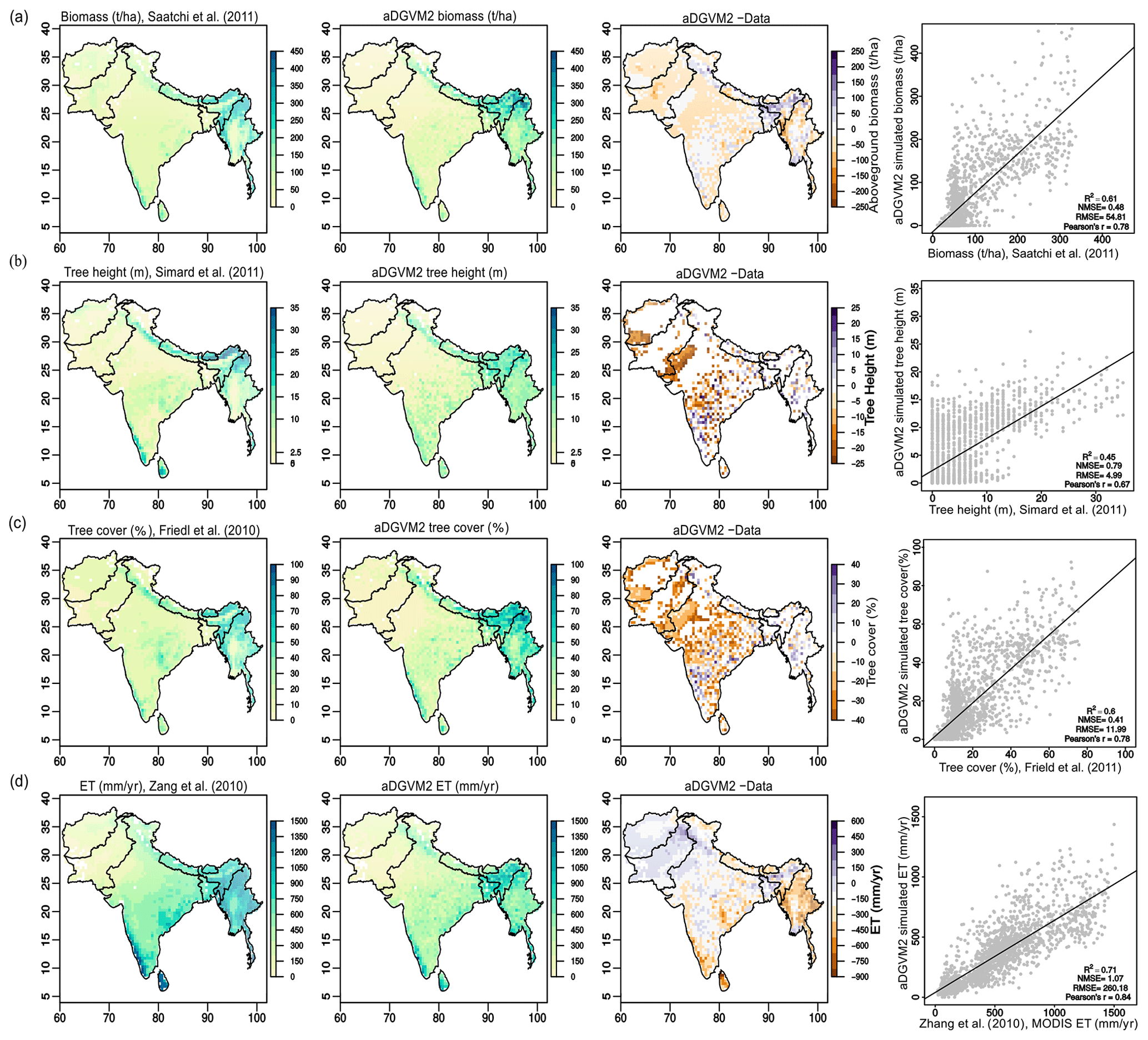
Figure 1 Comparison between aDGVM2 results and data for (a) simulated biomass and Saatchi et al. (2011) biomass, (b) simulated tree height and Simard et al. (2011) tree height, (c) simulated tree cover and Friedl et al. (2011) tree cover, and (d) simulated evapotranspiration and Zang et al. (2010) evapotranspiration. In the figure the first column shows the remote sensing products, the second column shows aDGVM2 results, the third column shows the difference between simulation and data, and the fourth column shows the scatter plot between simulated state variables against benchmarking data. NMSE and RMSE are the normalized mean square error and root mean square error, respectively. In the fourth column, each point represents one grid cell in the study region. For results with masked land-use cover see Supplement Fig. S4.

2.6 Biome classification

The aDGVM2 simulates state variables such as biomass and canopy cover of individual plants in simulated vegetation stands (1 ha, which is a representative of a grid cell). We used woody canopy area, abundance of shrubs and trees, and grass biomass to classify the simulated vegetation into biome types (Fig. S5). We used 10-year averages of state variables for the periods 2000–2009, 2050–2059 and 2090–2099 to represent the 2000s, 2050s and 2090s, respectively. We classified areas with woody canopy cover below 5 % as barren if grass biomass was below 100 kg/ha and as grassland if grass biomass exceeded 100 kg/ha. Grassland was classified as C₃ grassland or C₄ grassland based on predominance of C₃ or C₄ grass biomass. Simulated woody individuals were classified as trees if they had three or less stems and as shrubs if they had four or more stems (see Supplement). The canopy cover of woody plants and grass biomass was used to separate woodland and savanna biomes. Grid cells with tree canopy cover greater than shrub canopy cover, tree canopy cover between 5 % and 45 %, and grass biomass below 100 kg/ha were classified as woodland. Grid cells with the same woody cover characteristics but grass biomass higher than 100 kg/ha were classified as savanna. Savanna was further separated into C₃ savanna and C₄ savanna based on the predominance of C₃ or C₄ grass biomass. Areas with canopy cover greater than 45 % were classified as forest if tree cover exceeded shrub cover or shrubland if shrub cover exceeded tree cover, irrespective of grass biomass. Forests were subdivided into evergreen and deciduous forest based on the dominance of canopy area of both tree phenology types. In aDGVM2, whether a plant is deciduous or evergreen is decided by a trait. Biomes considered in this study were hence C₃ grassland, C₄ grassland, shrubland, woodland, deciduous forest, evergreen forest, C₃ savanna and C₄ savanna.

Biomes differ in the amount of precipitation they receive and their temperatures. Whittaker plots describe the boundaries of observed biomes with respect to temperature and precipitation. We used the “plotbiomes” R package (https://github.com/valentinitnelav/plotbiomes by ) to create Whittaker plots based on Ricklefs (2008) and Whittaker (1975). We overlaid the simulated biomes on Whittaker plots to assess climatic niches of biomes under current climate to determine shifts in climatic niches by the end of this century as a result of climate change and elevated CO₂ under both RCPs (see Sect. 3.6).

2.7 Calculation of biome-level evapotranspiration

For analyzing evapotranspiration change we calculated the amount of water transpired per unit leaf biomass. Simulated ET and leaf biomass for woody plants, C₃ grass, and C₄ grass were summed and scaled to the grid level, taking latitudinal variation of grid cell area into account. Absolute change in evapotranspiration quantity can either result from the change in biome area, from a change in total amount of leaf biomass over time or from changes in water use efficiency. In order to eliminate the effects caused by change in biome area and leaf biomass, we calculated biome-level evapotranspiration by normalizing evapotranspiration with biome-level leaf biomass (Eq. 6). Due to the normalization, differences in evapotranspiration at the biome level are comparable between different biomes and independent from biome attributes such as spatial extent and biome-level biomass. The biome-level evapotranspiration is calculated as the ratio of total annual ET over total leaf biomass for all respective biomes:

$$\begin{array}{}\text{(6)}& E_{\mathrm{biome}}={\displaystyle \frac{{\sum }_{i=\mathrm{1}}^G\left(E_{\mathrm{grid},i}{A}_{\mathrm{grid},i}\right)}{{\sum }_{i=\mathrm{1}}^G\left(B_{\mathrm{grid},i}{A}_{\mathrm{grid},i}\right)}},\end{array}$$

where E_biome is biome-level ET (mm/kg/year), 1, 2, …, G represents the grid cells of the biome; A_grid,i is the area of grid cell i (m²); E_grid,i is the total evapotranspiration of grid cell i (mm/year); and B_grid,i is the leaf biomass of grid cell i (kg/m²). Choosing to normalize evapotranspiration to leaf biomass integrates over both increased water use efficiency and soil water availability constraints. It is therefore suitable to characterize overall change in the water balance over time at the biome level, as it not only indicates water used to produce new biomass (as gross primary production over transpiration would express), but also includes water required to sustain existing biomass. We calculated the percentage change in E_biome for respective scenarios between the 2010s and 2050s and between the 2010s and the 2090s.

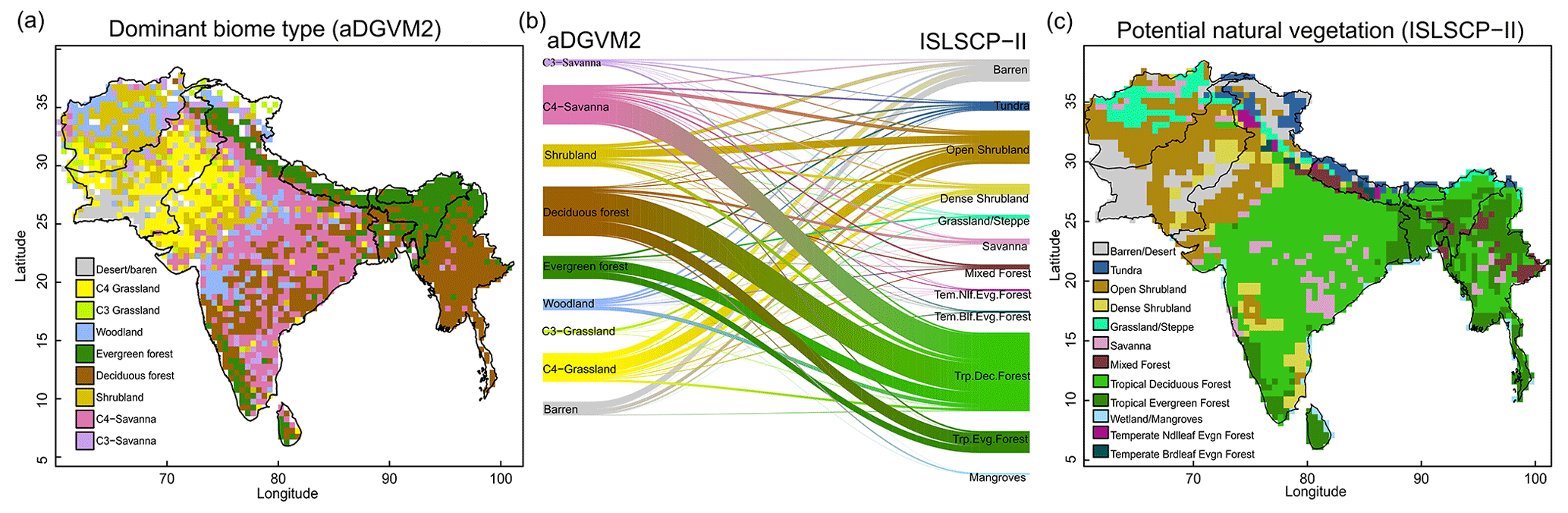
Figure 2 Comparison between simulated and observed biome patterns. (a) Simulated dominant biome type, (b) Sankey diagram showing overlap between simulated biomes and potential natural vegetation cover (ISLSCP II, Ramankutty et al., 2010), and (c) potential natural vegetation. The Sankey graph shows how aDGVM2 biomes and PNV classes overlap.

3 Results

3.1 Model performance and contemporary vegetation patterns

The aDGVM2 captured contemporary large-scale patterns of biomass, canopy cover, tree height and evapotranspiration. Model results agreed well with remote sensing products used for benchmarking (Figs. 1 and 2). R² was 0.61, 0.45, 0.6 and 0.71, and NMSE was 0.48, 0.78, 0.4 and 1.07 for biomass (Saatchi et al., 2011), tree height (Simard et al., 2011), tree cover (Friedl et al., 2010) and evapotranspiration (Zhang et al., 2010), respectively (Fig. 1). Data–model agreement improved when masking out managed land (Tuanmu and Jetz, 2014). R² increased to 0.66, 0.71, 0.67 and 0.80, while NMSE decreased to 0.43, 0.30, 0.61 and 1.03 for biomass, tree height, tree cover and evapotranspiration, respectively (Fig. S4). The model performed well in areas with higher fractional cover of natural vegetation, such as the Himalayas, Western Ghats and the northeast of the region, although the model overestimated biomass and canopy area in the Brahmaputra basin, which lies between 28–34^∘ N and 90–96.5^∘ E in the northeast of the study region (Fig. 1a, c,  Kumar et al., 2020).

The model simulated evergreen forests along the Himalayan mountains, the southern part of the Western Ghats and Sri Lanka, whereas deciduous forest was simulated in the northern Western Ghats, central India and the southern parts of Myanmar (Fig. 2a). Savanna was simulated in the southern, northern, and western parts of India and some regions of central Myanmar. Shrublands were simulated in the arid regions of Pakistan, the western parts of India and Afghanistan. The aDGVM2 simulated woodland in the west of central India and grassland in the drier regions (Fig. 2a). A large proportion of simulated deciduous forest area is in good agreement with that in maps of potential natural vegetation (PNV, Fig. 2b, c). However a large proportion of simulated savanna area is represented as deciduous forest in the map of PNV (Fig. 2b).

3.2 Projected changes in biome distribution pattern

The aDGVM2 projected increasing trends for canopy cover and aboveground biomass in response to climate change and CO₂ and hence changes in biome type, predominantly from savanna and grassland to deciduous forest (Fig. 3a, b). Simulations showed an increase in the area covered by evergreen and deciduous forests under both scenarios with eCO₂, in contrast to simulations under both scenarios with fCO₂, where CO₂ was fixed after 2005 (Table 1). Under RCP4.5+eCO₂, evergreen and deciduous forest cover increased by 3.1 % and 21.2 % until the 2050s and by 38.0 % and 59.1 % until the 2090s, respectively. Under RCP8.5+eCO₂, evergreen and deciduous forest increased by 24.8 % and 45.4 % until the 2050s and by 46.5 % and 60.2 % until the 2090s, respectively. The model simulated a small increase in forest area for RCP4.5+fCO₂, where the area increased by 7.9 % and 14.4 % for evergreen and deciduous forest until the 2090s, respectively. Evergreen forests were mainly simulated along the Himalayas, Western Ghats and eastern parts of the study region under current conditions (2000s, Fig. 3a) but expanded into the south of peninsular India in future periods (2050s and 2090s) under RCP4.5+eCO₂. Deciduous forest cover also increased in future periods in central India and along the Himalayas (Figs. 3 and S6).

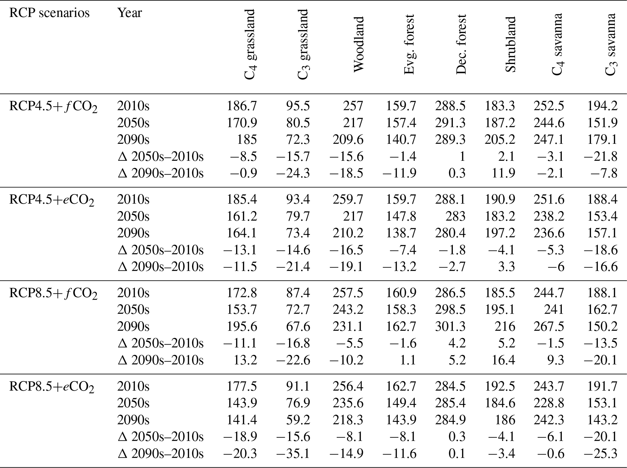
Table 1 Biome cover (in %) for the 2000s, 2050s and 2090s, and percent (%) change in biome cover from the 2000s to the 2050s and the 2000s to the 2090s under RCP4.5 and RCP8.5 with fixed and elevated CO₂. Δ indicates percent change in biome cover between time periods.

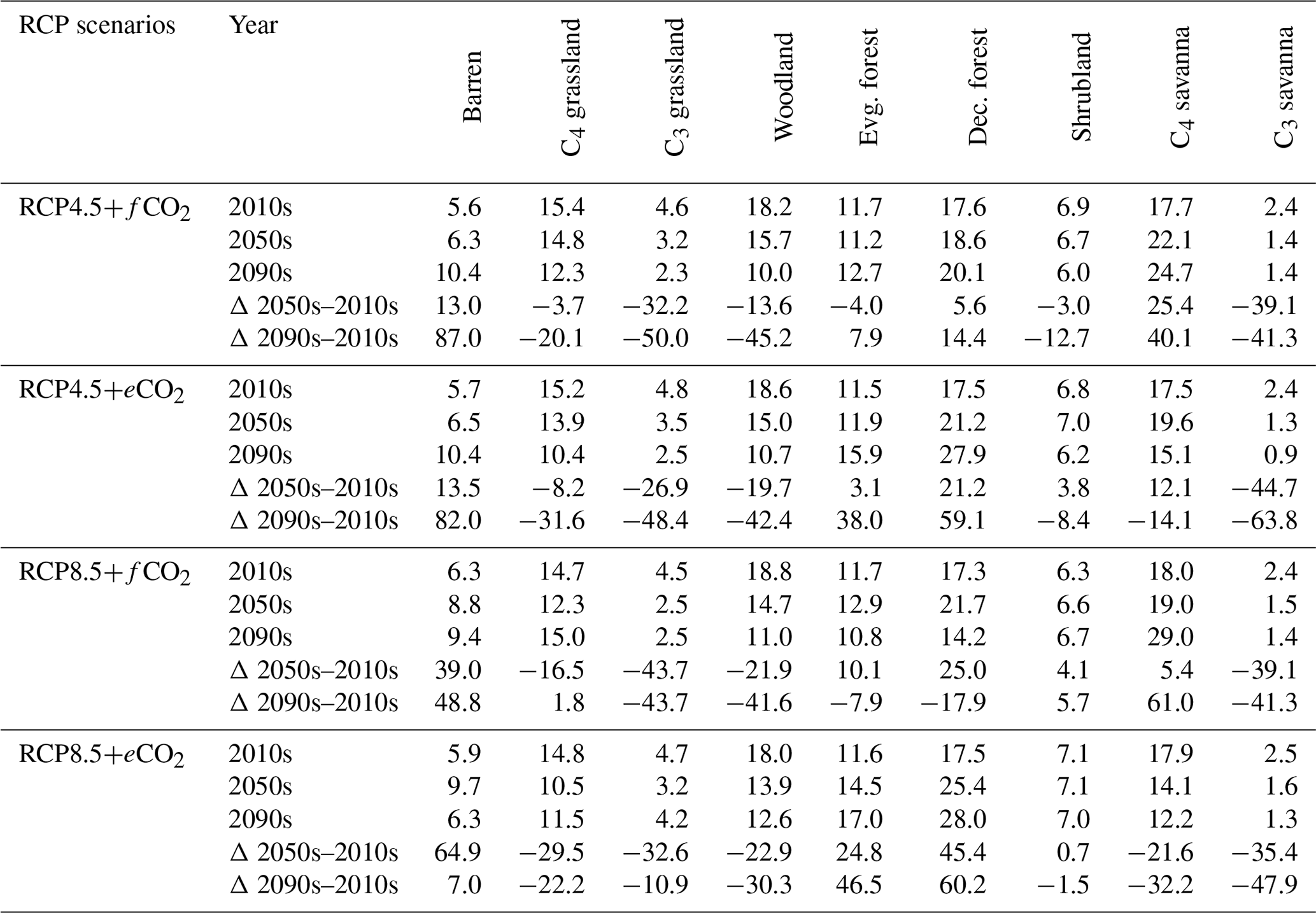
Figure 3 Simulated biome distribution for the 2000s, 2050s and 2090s under (a) RCP4.5+eCO₂ and (c) RCP4.5+fCO₂. The Sankey diagrams show the fractional cover of biomes and transitions between biomes from the 2000s to the 2050s and the 2050s to the 2090s under (b) RCP4.5+eCO₂ and (d) RCP4.5+fCO₂. See Fig. S6 for the simulated biome distribution under RCP8.5.

The extent of C₄ savanna showed a significant decrease under scenarios with eCO₂, although in RCP4.5+eCO₂ it showed an increase by 12.1 % between the 2010s and the 2050s (Table 1, Fig. 3). Simulated C₄ savanna area decreased by 14.1 % relative to the 2000s until the 2090s under RCP4.5+eCO₂. Under RCP8.5+eCO₂ the model projected a decrease in C₄ savanna area of 21.6 % and 32.2 % until the 2050s and the 2090s, respectively. The area covered by C₄ savanna increased under both RCPs with fCO₂ (Table 1). C₄ savannas were mainly located in the northern plain and peninsular India in the baseline period. However, these areas were replaced by deciduous forests in the northern plain and central India and by evergreen forests in peninsular India and in the southeast of the region by the 2090s under eCO₂ scenarios (Figs. 3a and S6a). The model simulated a decrease in area covered by woodland, shrubland, grasslands and C₃ savanna by the 2090s under all scenarios (Table 1, Fig. 3). Simulations showed an increase in barren areas in the western part of the region under all scenarios (Figs. 3 and S6, Table 1).

3.3 Projected changes in biomass at the biome level

The aDGVM2 predicted an increase in mean biomass for evergreen and deciduous forest in the eCO₂ scenarios for both RCPs (Table 2). Under RCP4.5+eCO₂, mean aboveground biomass in evergreen and deciduous forest increased by 8.1 % and 14.4 % by the 2050s and 3.8 % and 15.7 % by the 2090s, relative to the baseline period. The increase is even higher under RCP8.5+eCO₂ (Table 2). The mean biomass of woodland decreased under both RCPs except for the 2050s with eCO₂ scenarios. The mean biomass of grassland increased under RCP4.5 but decreased for C₄ grassland under RCP8.5 for both fCO₂ and eCO₂ scenarios. Shrublands in the western part of the study region showed an increase in mean biomass under eCO₂ scenarios except for the 2050s under both RCPs and a decrease under fCO₂ for both RCPs (Table 2). Our results showed that under RCP4.5 and RCP8.5 biomass decreased in the areas along the Himalayas, as well as in the central, northeastern and western parts of the study region by the end of the century. Modeled biomass decrease is higher under RCP8.5 in these regions (Figs. 4 and S7). Biomass in the central and southeastern part of the region is projected to increase under both RCPs with eCO₂ until the 2050s and 2090s and to decrease in southern India and in parts of western South Asia (Figs. 4 and S7). We found increased biomass in Afghanistan, western Pakistan, Nepal, and the southern part of Myanmar and decreased biomass in the western arid part of the study region under both RCPs for both eCO₂ and fCO₂ (Fig. 5), though the magnitude of change is different (Figs. 4 and S7). There were few areas in the western part of the study region where the model predicted increased biomass only under fCO₂ for both RCPs (Fig. 5). In large parts of the study region, biomass increased under eCO₂ for both RCPs but decreased under fCO₂; that is, CO₂ fertilization compensates for climate-change-induced biomass diebacks in these regions (Fig. 5).

Table 2 Mean biomass (in t/ha) within biomes for the 2000s, 2050s and 2090s, and percent (%) change in biomass from the 2000s to the 2050s and the 2000s to the 2090s under RCP4.5 and RCP8.5 with fixed and elevated CO₂. Δ indicates percentual biomass changes between time periods.

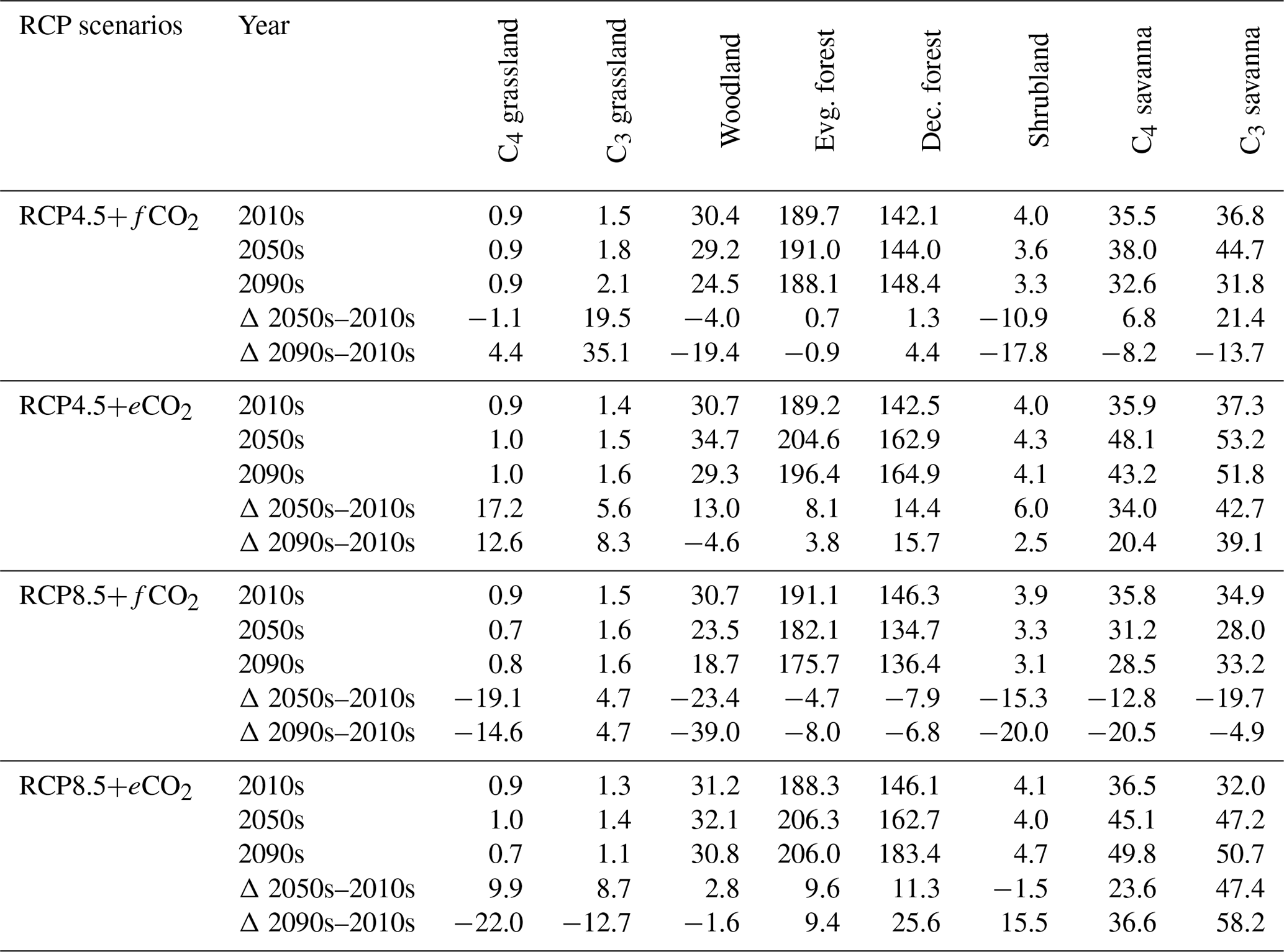
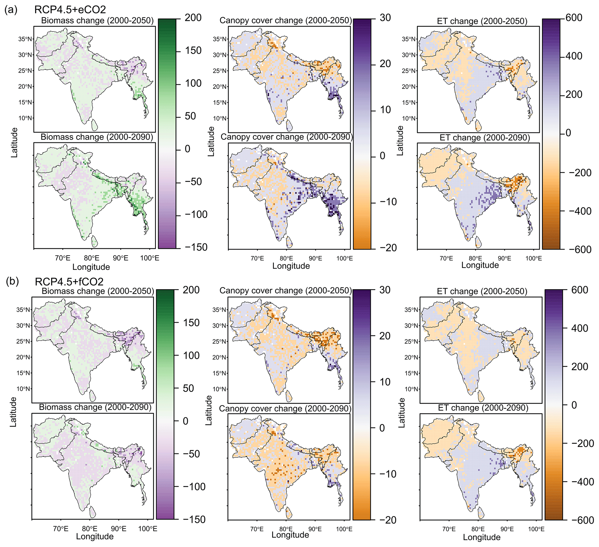
Figure 4 Projected change in biomass (t/ha), canopy cover (%) and evapotranspiration (ET, mm/year) between the 2000s and 2050s and between the 2000s and the 2090s under (a) RCP4.5+eCO₂ and (b) RCP4.5+fCO₂. See Fig. S7 for projected change of these variables under RCP8.5.

Figure 5 Maps showing areas where CO₂ fertilization compensates for biomass dieback caused by climate change between the 2000s and the 2090s under (a) RCP4.5 and (b) RCP8.5 and (c) aboveground biomass between 1950 and 2099 for South Asia in different scenarios.

3.4 Projected changes in evapotranspiration at the biome level

The response of simulated E_biome varies in different biomes under both RCP4.5 and RCP8.5 (Table 3). Under the RCP4.5+fCO₂ scenario the model predicted a decrease in ET in all biomes except for deciduous forest and shrubland where it increased by 1 % and 2.1 % until the 2050s and by 0.3 % and 11.9 % by the 2090s, respectively. Simulated E_biome under RCP8.5+fCO₂ for deciduous forest and shrubland increased by 4.2 % and 5.2 % until the 2050s and by 5.2 % and 16.4 % until the 2090s, respectively. The model also predicted increased E_biome for C₄ grassland, evergreen forest and C₄ savanna until the 2090s under RCP8.5+fCO₂ (Table 3). Comparisons of the RCP4.5+fCO₂ and RCP8.5+fCO₂ scenarios indicated that the former had a higher E_biome than the latter scenario across all biomes because precipitation decrease is higher in the RCP8.5 scenario than in the RCP4.5 scenario. Under both RCPs with eCO₂, the model predicted a decrease in E_biome across all biomes, except for a marginal increase in shrubland under RCP4.5 and deciduous forest under RCP8.5 until the 2050s and the 2090s (Table 3). In general, scenarios with eCO₂ showed lower biome-specific evapotranspiration across most of the biomes compared to simulations with fCO₂.

Table 3 Biome-level ET normalized to biomass (E_biome, mm/kg/year) for the 2000s, 2050s and 2090s, and percent (%) change in E_biome from the 2000s to the 2050s and the 2000s to the 2090s under RCP4.5 and RCP8.5 with fixed and elevated CO₂. Δ indicates percentual ET changes between time periods.

3.5 Response of mean ET and mean aboveground biomass to climate change

The model predicted a larger increase in absolute annual mean ET (mm/year) under eCO₂ than fCO₂ for both RCP scenarios due to the corresponding increase in biomass (Figs. 4 and S7). We compared the spatially averaged annual values over all of South Asia of simulated absolute ET with MAP over the period from 1951 to 2099 and found a statically significant relation (p value < 0.005). We found that absolute ET was positively correlated with MAP under all four scenarios (Figs. 6a and S8a) but weakly correlated with MAT (Figs. 6b and S8b). For a given MAP, the spatially averaged annual value of aboveground biomass (AGBM) was lower in scenarios with fCO₂ than scenarios with eCO₂ under both RCPs (Figs. 6c and S8c). The spatially averaged annual value of AGBM decreased beyond a MAT of 23.5 ^∘C for both RCPs with fCO₂, whereas it increased beyond 23.5 ^∘C under both RCP scenarios with eCO₂ (Figs. 6d and S8d).

Figure 6 Relationship between (a) evapotranspiration (ET) and mean annual precipitation (MAP), (b) ET and mean annual temperature (MAT), (c) mean aboveground biomass and MAP, and (d) mean aboveground biomass and MAT under RCP4.5. The lines (both solid and dotted) in all figures represent the best-fit regression line. Data points represent spatially averaged ET (a, b) and biomass (c, d) over all of South Asia for each year from 1950 to 2099. See Fig. S8 for results under RCP8.5.

3.6 Impact of climate change on climatic niches of biomes

The climate niches of simulated biomes broadly overlapped with the biome niches in the Whittaker scheme (Figs. 7 and S9, Ricklefs, 2008; based on Whittaker, 1975). Under RCP4.5+eCO₂ and RCP8.5+eCO₂, the aDGVM2 simulated shifts of climatic niches of biomes. Evergreen and deciduous forest biomes were predicted to invade the niche space of savannas under eCO₂ scenarios (Figs. 7 and S9). Savannas in turn were predicted to expand their climatic niche to MAT > 30 ^∘C by 2099, a climatic space that was essentially not occupied by current biomes. Under RCP8.5+eCO₂ in the 2090s, forests completely occupied the climate space, which is currently occupied by savanna (Fig. S9).

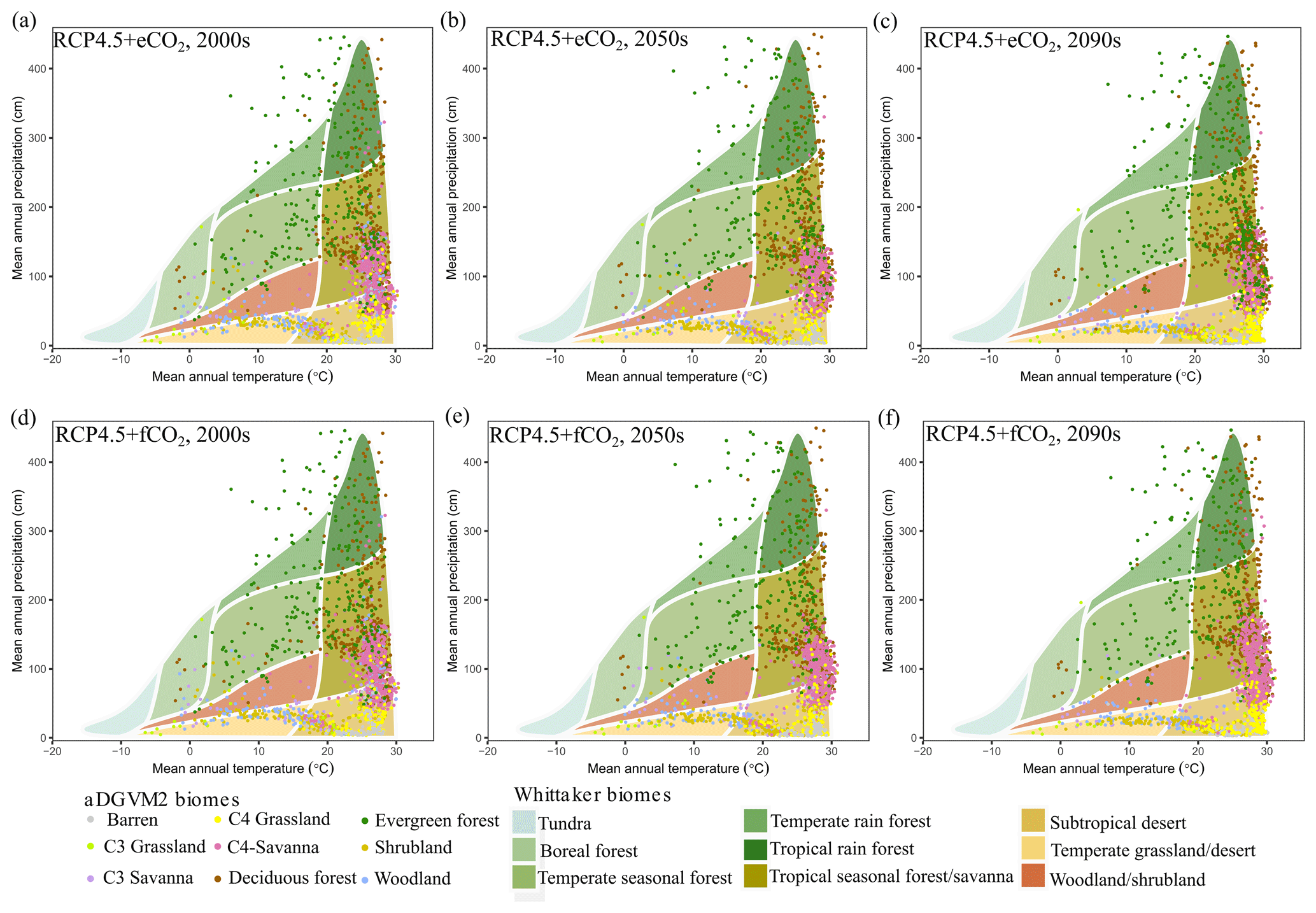
Figure 7 Simulated climate niches of biomes for the (a) 2000s, (b) 2050s and (c) 2090s under RCP4.5+eCO₂ and (d) 2000s, (e) 2050s and (f) 2090s under RCP4.5+fCO₂. The simulated biomes are overlaid on the climate envelopes of Whittaker's biomes and are plotted following Ricklefs (2008) and Whittaker (1975). See Fig. S9 for projected change in climatic niches of biomes under RCP8.5.

In both scenarios with fCO₂, savanna occupied the climate space delineated by MAT > 25 ^∘C and MAP between 500 and 1500 mm and did not experience major replacement by forest. The model predicted that savanna expansion in climate space was higher under RCP8.5+fCO₂ than under RCP4.5+fCO₂ (Figs. 7 and S9). Other biomes also experienced shifts in their climate space (Fig. 7). However, the results showed that for both the current and future period, grasslands and shrublands occupied the region with low MAP (<500 mm), and woodland occupied low MAP (<800 mm) regions, which correspond to the western arid and semiarid regions of the study region under the scenario with eCO₂ (Fig. 7).

4 Discussion

4.1 Impact of climate change and elevated CO₂ on biomes and biomass

Our simulations for RCP4.5+eCO₂ and RCP8.5+eCO₂ showed a strong positive response of vegetation growth, i.e., increases in biomass, canopy cover and canopy height. Mean biomass in most biomes was projected to increase, but the magnitude of increase differed considerably between different scenarios (Table 2). Projected change in canopy cover resulted in biome transitions. Under future conditions, the spatial distribution, extent and biomass of evergreen forests mostly remained at the current state, and evergreen forests were more resistant to climate change than deciduous forests. Expansion of deciduous forest into open biomes due to increasing woody cover resulted in significant loss of savanna area in the Deccan region under both RCPs with eCO₂ by the end of the century. Transition from deciduous forests to evergreen forest was simulated for the mountain regions of South Asia (Scheiter et al., 2020), i.e., the Himalayas and the Western Ghats, where precipitation was predicted to increase. The trade-offs between specific leaf area (A_SLA) and leaf longevity (LL) result in the emergence of evergreen behavior in wet regions of South Asia. In the wet tropics, higher LL allows achieving a constant positive carbon balance from photosynthesis throughout the year and increases the residence time of nutrients and carbon in the plant and therefore enhances the photosynthetic gain per unit carbon and nutrient investment in leaves (Kikuzawa and Lechowicz, 2011). The deciduous behavior is advantageous in dry regions, as in the Deccan region, because trees that do not invest much carbon into their leaves per unit dry mass (higher A_SLA and lower LL) lose less investment when shedding them during the dry season. Phenology change as a result of climate change has already been observed (Buitenwerf et al., 2015; Cleland et al., 2007). In Scheiter et al. (2020), we showed that climate change supports transitions to tall evergreen vegetation in tropical Asia and found increases in the abundance of evergreen plants and decreases in the abundance of deciduous plants in mainland Southeast Asia, central India and Pakistan. This relative advantage of evergreen plants over deciduous plants under elevated CO₂ in aDGVM2 can be explained by the fact that increased intrinsic water use efficiency under eCO₂ in evergreen plants is higher than in deciduous plants as demonstrated by Soh et al. (2019). Previous modeling studies also support aDGVM2 result showing transitions from deciduous to evergreen vegetation. With the BIOME4 model, Ravindranath et al. (2006) simulated the response of forest to Special Report on Emissions Scenarios (SRES) A2 and B2 and reported similar changes toward evergreen phenology. A study by Chaturvedi et al. (2011) using the IBIS model also predicted transitions toward evergreen forest.

Woody encroachment in many ecosystems is attributed to rising CO₂, and this is supported by studies based on both field observations (e.g., FACE experiments) and satellite data (Brienen et al., 2015; Fischlin et al., 2007; Piao et al., 2006; Schimel et al., 2015; Archer et al., 2017; Stevens et al., 2017). The aDGVM2 also supports these findings, i.e., increasing canopy cover and woody biomass under the eCO₂ condition, and agrees with the reported greening trend in South Asia during the last three decades (Wang et al., 2017). Elevated CO₂ affects plants by increasing their photosynthetic rate, growth rate and water use efficiency, leading to an increase in biomass (Leakey et al., 2009; Norby and Zak, 2011). Increased photosynthetic rates under elevated CO₂ are due to an increase in the rate of rubisco carboxylation for C₃ plants, with a concurrent decrease in photorespiratory losses of carbon (Long et al., 2004). Due to the improved carboxylation efficiency, C₃ plants can respond by reducing stomatal conductance, thereby reducing transpirational losses, improving leaf water status and water use efficiency, and favoring leaf area growth (Long et al., 2004; Norby and Zak, 2011). Evidence from both observation and modeling of forest dynamic suggests that combined effects of eCO₂ and increased water use efficiency include increases in forest growth and canopy greening, as well as widespread increases in woody plant biomass and potential forest carbon sink. However, it is still unclear how the CO₂ responses scale to the ecosystem level (Hickler et al., 2015) and how nutrient limitation from the soil may influence ecosystem responses to eCO₂. Körner (2015) argued that carbon from the atmosphere can only be converted into biomass if other factors such as nutrients, temperature and water are not limiting. In addition, the benefit of eCO₂ can be downregulated by broad-scale forest die-off due to frequent drought and warmer temperature (Choat et al., 2018; Mcdowell et al., 2016), as well as tree mortality due to negative tree physiological responses, negative carbon balance and accelerated pest attacks. Rising background mortality rates combined with projected increases in intensity, frequency and duration of drought (Huang et al., 2016) increase the uncertainty regarding positive effects of eCO₂.

In the long run, whether ecosystems act as a carbon source or sink can be estimated using models that consider all factors that are relevant in the carbon cycle and its associated factors (Fatichi et al., 2014; Körner, 2015). However, Terrer et al. (2019) showed that the global-scale response to eCO₂ from experiments is similar to past changes in greenness (Piao et al., 2019) and biomass (Sitch et al., 2015) in response to eCO₂. This suggests that CO₂ will likely continue to stimulate plant biomass in the future despite the constraining effect of soil nutrients; however Terrer et al. (2019) also argued that the empirical relationships with soil nutrients can be powerful for explaining large-scale patterns of eCO₂ responses, despite ecosystem-level uncertainties. According to our simulations we can conclude that natural vegetation of South Asia likely will remain a carbon sink in the future (Fig. 5).

4.2 Impact of climate change and fixed CO₂ on biomes and biomass

Under both fCO₂ scenarios, the spatial distribution of savanna areas remained in its contemporary state. Central India and the Deccan Plateau showed a transition of deciduous forest to savanna, because forest canopy opened up due to tree mortality caused by increasing temperature and reduced MAP. This indicates that plants experience temperature and drought stress under fixed CO₂. These stresses were compensated for by CO₂ fertilization in eCO₂ scenarios where the aDGVM2 simulated increased biomass and woody encroachment in areas affected by climate-induced dieback in fCO₂ simulations. This aDGVM2 behavior agrees with results presented by Lapola et al. (2009), who modeled biome shifts from forest to savanna in the absence of CO₂ fertilization for the Amazon region. Changes in precipitation regimes are likely to have a strong influence particularly in arid and semi‐arid regions, such as grasslands (Verstraete et al., 2009). The complex interactions of inter-annual precipitation variability and precipitation seasonality can result in rapid ecosystem transitions (e.g., between alternative stable states with high and low vegetation biomass; Holmgren and Scheffer, 2001). The decrease in simulated AGBM after MAT increases beyond 23.5 ^∘C under fCO₂ scenarios can be explained by the longer exposure of vegetation to temperatures beyond the optimum temperature range of C₃ photosynthesis during the main growing season. This effect was further enhanced by decreasing MAP and the absence of CO₂ fertilization. This implies that the increase in MAT above 23.5 ^∘C together with weak CO₂ fertilization would have negative consequences for carbon sequestration. The sensitivity of biomass to temperature and CO₂ change has been investigated in many studies (Norby and Luo, 2004; Song et al., 2019; Sperry et al., 2019). A meta-analysis by Lin et al. (2010) showed that warming significantly increased biomass by 12.3 % (with a 95 % confidence interval of 8.4 %–16.3 %) across all the terrestrial plants included. This observation is consistent with our model results. Biomass showed a positive relation with MAT, which did not change with mean annual precipitation or experimental duration or CO₂ enrichment (Lin et al., 2010). These findings are also supported by previous studies by Rustad et al. (2001), Walker et al. (2006), and Dormann and Woodin (2002), which have revealed that warming generally increases terrestrial plant biomass, indicating enhanced terrestrial carbon uptake via plant growth. Previous modeling studies using Biome‐BGC (Running and Hunt Jr, 1993), Century (Parton et al., 1993) and TEM (Tian et al., 1999) have shown an increase in productivity when both climate change and CO₂ effects were considered. However, the increase was smaller when only climate change effects were considered, and both Biome‐BGC and TEM suggest that without CO₂ fertilization, average productivity would decline relative to the current annual average as shown by our result (Fig. 6d). This suggests complexity and challenges in seeking general patterns of terrestrial plant growth in a future warmer climate condition. It also implies that we need a better understanding of impacts of heat stress on vegetation and how it interacts with drought and CO₂ fertilization. It is also unclear to what degree thermal acclimation may counteract some of the negative effects on plant growth caused by higher temperatures (Lombardozzi et al., 2015).

4.3 Impact of climate change and CO₂ change on climatic niches of biomes

Elevated CO₂ has a major impact on the climatic niche space of biomes. Our simulations showed forest invasion into the niche space currently occupied by savanna by the end of the century. The expansion of forests to drier areas corresponds to a widening of their climate niche space under eCO₂. This expansion is mainly driven by eCO₂ and is corroborated by the fact that in the absence of CO₂ fertilization the climatic niche of biomes is stable; i.e., biomes occupy the same niche space under current and future conditions. These findings imply that the bioclimatic boundaries used to define biome niche space are not static but are specific for given CO₂ levels. Therefore, the thresholds of Whittaker's biomes need to be redefined for a high-CO₂ world such that they encompass the altered climatic envelopes of biomes under elevated CO₂ in the future (Fig. 7). The shift in niche space can be attributed to the shift in plant communities caused by the combined effect of climate change and elevated CO₂, which increases plant water use efficiency, allowing them to grow under drier conditions. These community shifts can also lead to a change in the characteristics of biomes by altering community structure and ecosystem functions (Chapin et al., 1997).

4.4 Effect of CO₂ on ET and its interaction with climate change

Climate change has direct effects on hydrological processes (Liu et al., 2008). ET and water deficit influence plant productivity and distribution (Stephenson, 1998). Higher biomass coincided with increased absolute amounts of ET for eCO₂ scenarios in some parts of the study region under both RCPs by the end 21st century (Figs. 5 and S7). This change can be attributed to higher leaf biomass accumulated in plants enabled by increased photosynthetic efficiency under eCO₂. The higher amount of leaf biomass offsets the water-saving effect caused by reduced stomatal conductance due to improved water use efficiency under eCO₂ scenarios and resulted in reduced ET per unit leaf biomass (Warren et al., 2011). Our results showed that the strength of the CO₂ fertilization effect is relevant when attempting to determine E_biome at the biome level during the 21st century. Biome-specific ET decrease was less pronounced under RCP4.5 due to a lower concentration of atmospheric CO₂ compared to RCP8.5. Our simulated decrease in ET in response to climate change and increasing CO₂ concentration agrees with Kergoat et al. (2002), who have reported decreased ET under elevated CO₂ concentration in a chamber experiment. However, reduced ET under eCO₂ can reduce regional-scale atmospheric humidity and thereby enhance the vapor pressure deficit (VPD) between leaves and atmosphere, a driving force for water loss, which may partially counteract CO₂-induced reduction of ET due to decreased stomatal conductance. Due to stomatal closure, photosynthetic rates under soil water stress conditions decline in aDGVM2 when atmospheric VPD increases. The projected increase in air temperature also increases the saturated water vapor pressure. As a result VPD will increase, given that increase in actual vapor pressure is limited by soil water availability while the increase in saturated vapor pressure is not (Yuan et al., 2019), and potential evapotranspiration will increase with temperature (Warren et al., 2011). As future climate projections vary spatially and temporally, there was high model uncertainty on how ET will respond to changes in precipitation and temperature.

4.5 Implication of the projected change for conservation

Changes in biome types imply changes in biodiversity, ecosystem function and productivity. Each biome is characterized by a range of distinctive ecological processes and functions. For instance, the distribution of forest ecosystem in the mountains is largely regulated by the altitude and climatic factors (Saikia et al., 2017). They have high species richness and needed to be protected from the ever-increasing anthropogenic pressure and climate change. Open biomes such as grassland and savanna support high biodiversity (Parr et al., 2014). Pronounced increases in tree density in grasslands and savannas will alter vegetation structure and reduce grassland biodiversity. Such changes will negatively affect savanna-specific ecosystem services such as grazing potential, tourism and wildlife habitat availability (Parr et al., 2012). The threat posed to the biodiversity of Asian savannas by climate change is aggravated by inadequate management policies that misinterpret them as degraded forest (Ratnam et al., 2016). In this context, management policies aim to afforest open biomes, although paleoecological evidence indicates that these open biomes are not degraded forest but ancient ecosystems (Kumar et al., 2020; Ratnam et al., 2016). Moreover, increased woody cover can negatively affect water resources in the semiarid regions of the study area. Acharya et al. (2018) have shown that increased woody cover hinders the downward movement of water, causing increased water inception, which has negative effects on groundwater recharge. It is therefore necessary to control the abundance of woody plants in semiarid regions to control stream flow and enhance groundwater recharge (Bednarz et al., 2001).

In South Asia, biodiversity hotspots have a very unique topography, where climate varies strongly over short distances. As global biodiversity hotspots, mountain forest ecosystems in the Western Ghats, the Himalayas and northeastern part of the study area (India and Myanmar) are particularly vulnerable to climate change (Myers et al., 2000) and need targeted management action to mitigate adverse effects. Conservation of these hotspots requires consideration of many different attributes of plant communities, ecosystems, landscapes, and plant diversity; of how they will change; and of how their ecosystem services are valued.

Conservation methods and policies that can accommodate minimal losses of ecosystem services and provide robust strategies to mitigate climate change impacts should be developed and implemented. In this context, DGVMs facilitate the exploration of vegetation–climate interactions by providing detailed results for different management and climate scenarios. Such an exploration of different possible scenarios is necessary to develop optimized mitigation and conservation strategies for protected areas in biodiversity hotspots. The value of DGVM modeling results lies in their potential to provide insights into multiple future trajectories. Based on the most likely trajectories, the results can be used to tailor best-practice strategies for decision makers that need to manage conservation areas or protected areas (Boulangeat et al., 2012).

4.6 Limitations of this modeling study

Our simulation results are constrained by the model formulation and the assumptions underlying aDGVM2. Disagreement between model results and data used for benchmarking can be attributed to the fact that the aDGVM2 simulates potential natural vegetation, whereas remote sensing products integrate land use. This implies that enhancing the model to simulate observed land cover patterns would require additional information on anthropogenic impacts. Anthropogenic activities such as deforestation, habitat conversion and urbanization can modify the interactions between climate, plant communities and biomes (Hansen et al., 2001).

In addition data–model disagreement can be explained by model uncertainties and processes currently not considered in aDGVM2. For instance, aDGVM2 uses carbon allocation parameters that are not easily measurable in the field, which limits the evaluation of simulated mechanisms. The model currently does not account for carbon that plants invest into nutrient acquisition (e.g., mycorrhiza) or into defenses against predation and pathogens (Zemunik et al., 2015). There is insufficient ecophysiological data from the study region, which are required for parameterization of trait ranges used to simulate regional plant communities (Kumar and Scheiter, 2019). The complexity of the interactions between global change and biomes as well as biodiversity is difficult to model in the absence of such data. While the model currently captures effects related to CO₂ fertilization and temperature, associated mortality reasons such as pests attack and heat damage to plant tissues are insufficiently represented in the models. The low resolution of input data, both soil and climate data, also limits the model's capability to capture high-resolution regional heterogeneity in vegetation distribution. Further, the strength of CO₂ fertilization modeled in aDGVM2 may be overestimated because the effect of nutrient limitation on productivity is not included in this version of aDGVM2 (Körner et al., 2005; Terrer et al., 2018). Despite these caveats, we are nonetheless confident in capturing general patterns of future global change and its consequences for biomes and their boundaries in South Asia.

5 Conclusions

The model reproduced the contemporary distribution of biomes, biomass, evapotranspiration and tree height. We investigated the impact of eCO₂ and climate change on South Asian biomes and found that climate change and CO₂ fertilization in combination are substantial drivers of biome change and that elevated CO₂ concentrations altered the climatic envelope of biomes in addition to causing increases in biomass, tree height and canopy cover. Continued biomass increase indicates that South Asia's natural vegetation will likely remain a carbon sink in the 21st century. Our results also imply that woody encroachment poses a threat to open biomes and causes the transition of savanna biomes to deciduous forest in the future. The savanna biome is important in the context of biodiversity conservation. We showed that bioclimatic niches of biomes are not static but are specific for given CO₂ concentrations. We therefore argue that Whittaker plots used to illustrate niches of biomes need to be adjusted for future climate conditions. We also found that the simulated decrease in biomass-specific ET is more pronounced in scenarios with eCO₂ than in scenarios with fCO₂, which indicates that water use efficiency will likely increase due to CO₂ fertilization.

The biome transitions simulated under eCO₂ and changing climate indicate the need to adjust ecosystem management, mitigation strategies and conservation policies for protected areas to allow targeted long-term management. To understand the significance of ecological responses to climate change, it is essential to improve and expand biological monitoring activities (Loreau et al., 2001). To achieve this, the most vulnerable biomes that we identified in this study could be proposed as high-priority targets for programs that monitor vegetation–climate interactions, productivity and biodiversity (Proença et al., 2017).