the Creative Commons Attribution 4.0 License.
the Creative Commons Attribution 4.0 License.
 | 27 May 2021
Ocean carbon cycle feedbacks in CMIP6 models: contributions from different basins
Anna Katavouta
Richard G. Williams
The ocean response to carbon emissions involves the combined effect of an increase in atmospheric CO2, acting to enhance the ocean carbon storage, and climate change, acting to decrease the ocean carbon storage. This ocean response can be characterised in terms of a carbon–concentration feedback and a carbon–climate feedback. The contribution from different ocean basins to these feedbacks on centennial timescales is explored using diagnostics of ocean carbonate chemistry, physical ventilation and biological processes in 11 CMIP6 Earth system models. To gain mechanistic insight, the dependence of these feedbacks on the Atlantic Meridional Overturning Circulation (AMOC) is also investigated in an idealised climate model and the CMIP6 models. For the carbon–concentration feedback, the Atlantic, Pacific and Southern oceans provide comparable contributions when estimated in terms of the volume-integrated carbon storage. This large contribution from the Atlantic Ocean relative to its size is due to strong local physical ventilation and an influx of carbon transported from the Southern Ocean. The Southern Ocean has large anthropogenic carbon uptake from the atmosphere, but its contribution to the carbon storage is relatively small due to large carbon transport to the other basins. For the carbon–climate feedback estimated in terms of carbon storage, the Atlantic and Arctic oceans provide the largest contributions relative to their size. In the Atlantic, this large contribution is primarily due to climate change acting to reduce the physical ventilation. In the Arctic, this large contribution is associated with a large warming per unit volume. The Southern Ocean provides a relatively small contribution to the carbon–climate feedback, due to competition between the climate effects of a decrease in solubility and physical ventilation and an increase in accumulation of regenerated carbon. The more poorly ventilated Indo-Pacific Ocean provides a small contribution to the carbon cycle feedbacks relative to its size. In the Atlantic Ocean, the carbon cycle feedbacks strongly depend on the AMOC strength and its weakening with warming. In the Arctic, there is a moderate correlation between the AMOC weakening and the carbon–climate feedback that is related to changes in carbonate chemistry. In the Pacific, Indian and Southern oceans, there is no clear correlation between the AMOC and the carbon cycle feedbacks, suggesting that other processes control the ocean ventilation and carbon storage there.
- Article
(14867 KB) - Full-text XML
-
Supplement
(807 KB) - BibTeX
- EndNote


Carbon emissions drive an Earth system response via direct changes in the biogeochemical carbon cycle and the physical climate. These changes in the biogeochemical carbon cycle and physical climate further amplify or dampen the Earth system response, with this amplification often referred to as a feedback (Sherwood et al., 2015). The physical climate feedback involves the combined effect from changes in atmospheric water vapour, tropospheric lapse rate, surface albedo and clouds (Ceppi and Gregory, 2017) and from a shift in the regional patterns of ocean heat uptake due to changes in the ocean circulation (Winton et al., 2013). For the carbon cycle, an initial increase in atmospheric CO2 leads to carbon uptake and storage in land and ocean reservoirs. This response of the carbon cycle to the increase in atmospheric CO2 is characterised by the carbon–concentration feedback. At the same time, the carbon cycle is further modified by changes in the physical climate, such as warming and an increase in ocean stratification leading to an amplification of the initial increase in atmospheric CO2. This response of the carbon cycle to changes in the physical climate is characterised by the carbon–climate feedback. These two carbon cycle feedbacks have been extensively used to understand and quantify the response of the global carbon cycle to carbon emissions (Friedlingstein et al., 2003, 2006; Gregory et al., 2009; Boer and Arora, 2009; Arora et al., 2013; Schwinger et al., 2014; Schwinger and Tjiputra, 2018; Williams et al., 2019; Arora et al., 2020). A regional extension of the carbon cycle feedbacks has been also used to explore their geographical distribution and the mechanisms that control the land and ocean carbon uptake and storage in difference regions (Yoshikawa et al., 2008; Boer and Arora, 2010; Tjiputra et al., 2010; Roy et al., 2011).
On a global scale, the carbon–concentration feedback is of comparable strength over the land and ocean, while the carbon–climate feedback is about 3 times stronger over the land than over the ocean on centennial timescales in the CMIP6 Earth system models (Arora et al., 2020). However, there is a substantial geographical variation in the ocean carbon–climate feedback (Tjiputra et al., 2010; Roy et al., 2011) as a result of an interplay between the effect of carbonate chemistry, physical ventilation and biological processes. In the tropics, the carbonate chemistry and the decrease in solubility with warming drives a reduction in the ocean carbon uptake with climate change (Roy et al., 2011; Rodgers et al., 2020). In the North Atlantic, the physical ventilation and its weakening with warming acts to further reduce the ocean carbon uptake with climate change (Yoshikawa et al., 2008; Tjiputra et al., 2010; Roy et al., 2011). In the Southern Ocean, changes in the cycling of biological material with climate change can partly counteract the reduction in the ocean carbon uptake due to the decrease in solubility and physical ventilation with warming (Sarmiento et al., 1998; Bernardello et al., 2014).
The ocean carbon cycle feedbacks can be defined in terms of either the cumulative ocean carbon uptake or the ocean carbon storage (Schwinger et al., 2014; Arora et al., 2020). For the global ocean, these two definition are almost equivalent apart from a small contribution from the land-to-ocean carbon flux from river runoff and the carbon burial in ocean sediments (Arora et al., 2020). However, on a regional scale these two definitions are different, as the ocean carbon storage explicitly includes the convergence of transport of carbon by the ocean circulation. This transport effect leads to different geographical patterns for the ocean carbon storage and the ocean cumulative carbon uptake (Frölicher et al., 2015). This transport effect also leads to a broadly similar geographical distribution for ocean carbon and heat storage, with the “redistribution” of the pre-industrial carbon and heat by changes in the circulation with warming driving a second-order asymmetry between the regional patterns of heat and carbon storage (Winton et al., 2013; Bronselaer and Zanna, 2020; Williams et al., 2021). The combined air–sea transfer and transport effect leads to the Atlantic, Pacific and Southern oceans each storing about 25 %–30 % of the additional heat and carbon in CMIP6 models for a quadrupling of atmospheric CO2 (Fig. 1a and b), despite their different sizes (see Supplement Fig. S1 for the basins' definition). The Atlantic and Arctic oceans have the largest increase in carbon and heat per unit volume, as given by the dissolved inorganic carbon and temperature (Fig. 1c and d). The Pacific Ocean has the smallest increase in carbon and heat per unit volume (Fig. 1c and d). Our motivation is to explore the mechanisms that lead to these regional variations in carbon storage and carbon cycle feedbacks in the different ocean basins in CMIP6 models.
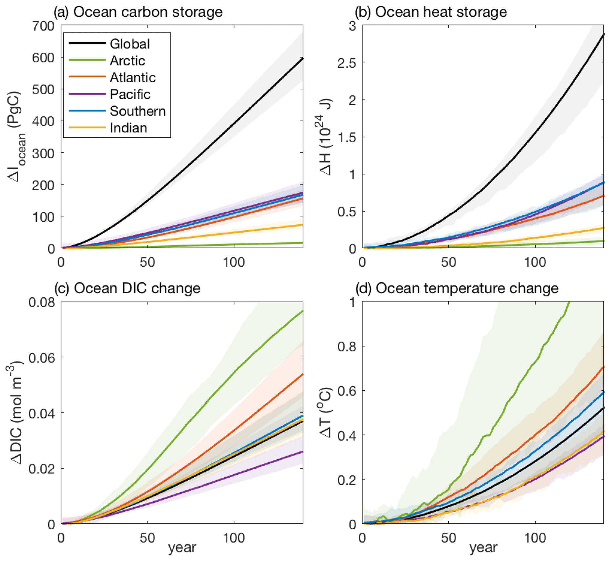
Figure 1Carbon and heat storage for the global ocean and different ocean basins in CMIP6 Earth system models: (a) ocean carbon content changes relative to the pre-industrial in petagrams of carbon; (b) ocean heat content changes relative to the pre-industrial in joules; (c) changes in the ocean dissolved inorganic carbon relative to the pre-industrial in moles per cubic metre, expressing the ocean carbon storage changes per volume; and (d) changes in ocean temperature relative to the pre-industrial in degrees Celsius, expressing the ocean heat changes per volume. The solid lines show the model mean and the shading the model range based on the 1 % yr−1 increasing CO2 experiment over 140 years in 11 CMIP6 models (Table 1). For the definition of the ocean basins see Supplement Fig. S1.
A mechanism that can affect the regional carbon storage is the Atlantic Meridional Overturning Circulation (AMOC). The projected weakening in the AMOC with climate change (Cheng et al., 2013) weakens the ocean physical ventilation and transport of carbon into the ocean interior, which acts to reduce the ocean carbon uptake and storage (Sarmiento and Le Quéré, 1996; Crueger et al., 2008). The weakening in the AMOC with climate change also increases the residence time in the ocean interior and the accumulation of remineralised carbon at depth, which acts to increase the ocean carbon uptake and storage (Sarmiento and Le Quéré, 1996; Joos et al., 1999; Schwinger et al., 2014; Bernardello et al., 2014). Previous studies suggest that the combined effect of these two competing processes leads to a modest reduction in ocean carbon uptake and storage with AMOC weakening and to an ocean carbon–climate feedback that amplifies the increase in atmospheric CO2 (Sarmiento and Le Quéré, 1996; Joos et al., 1999; Crueger et al., 2008; Schwinger et al., 2014). However, the net effect of AMOC weakening with climate change on the carbon storage is highly uncertain and sensitive to the representation of the vertical carbon gradient and ocean biological processes in Earth system models. This uncertainty motivates us to explore the control of the AMOC on the carbon cycle feedbacks in CMIP6 models, as well as the relative importance of changes in biological processes and physical ventilation for the carbon storage in different ocean basins.
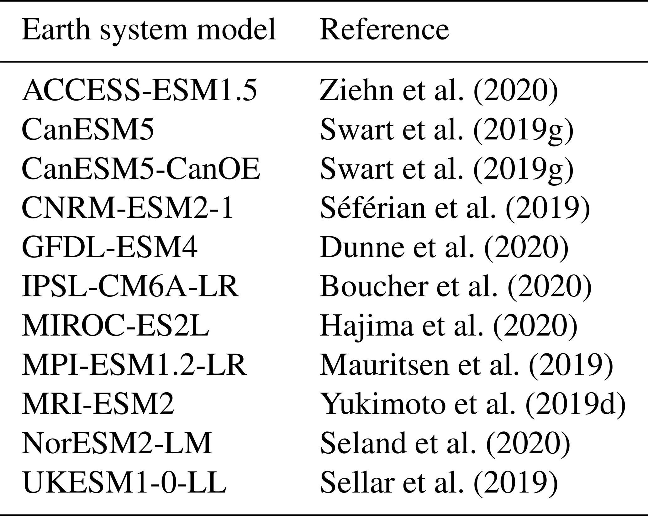
Our aim is to provide insight into the relative contribution of different ocean basins to the ocean carbon cycle feedbacks and the processes that drive this regional partitioning in the CMIP6 models. In Sect. 2, we provide the framework for the carbon cycle feedbacks and explore their geographical distribution in 11 CMIP6 Earth system models (Table 1). In Sect. 3, the ocean carbon cycle feedbacks are separated into contribution from carbonate chemistry, physical ventilation and biological processes, and the controls of the global and regional feedbacks are investigated in diagnostics of CMIP6 models. In Sect. 4, the effect of the AMOC on the global and basin-scale carbon cycle feedbacks is investigated, firstly using an idealised climate model that provides a mechanistic insight and then in diagnostics of CMIP6 models. Section 5 summarises our conclusions and discusses the wider context of our analysis.
Ziehn et al. (2020)Swart et al. (2019g)Swart et al. (2019g)Séférian et al. (2019)Dunne et al. (2020)Boucher et al. (2020)Hajima et al. (2020)Mauritsen et al. (2019)Yukimoto et al. (2019d)Seland et al. (2020)Sellar et al. (2019)Table 1List of the 11 CMIP6 Earth system models used in this study along with references for the model description.
2.1 Global ocean
In the carbon cycle feedback framework introduced by Friedlingstein et al. (2003, 2006) the ocean carbon gain due to anthropogenic carbon emissions, ΔIocean, is expressed as a function, F, of changes in the atmospheric CO2 and the physical climate:
where the surface air temperature, T, is used as a proxy for the physical climate and subscript 0 denotes the pre-industrial state. By expanding the function F into a Taylor series (Schwinger et al., 2014; Williams et al., 2019), the ocean carbon gain relative to the pre-industrial era, ΔIocean, is expressed as
where R3 contains the third-order and higher derivatives. By ignoring the second- and higher-order terms but keeping the terms for the non-linear relationship between atmospheric CO2 and climate change, Eq. (3) is rewritten as
where the ocean carbon–concentration feedback parameter is defined as , the ocean carbon–climate feedback parameter is defined as and the non-linearity of the ocean carbon cycle feedbacks is defined as .
The carbon cycle feedback parameters, β and γ, are traditionally estimated using Earth system model simulations with the couplings between the carbon cycle and radiative forcing switched either on or off: a fully coupled simulation, a radiatively coupled simulation and a biogeochemically coupled simulation (Friedlingstein et al., 2006; Arora et al., 2013; Jones et al., 2016; Arora et al., 2020). Any combination of these three simulations can be used to estimate the carbon cycle feedback parameters; however, each combination yields somewhat different results due to the non-linearity of the system (Gregory et al., 2009; Zickfeld et al., 2011; Schwinger et al., 2014; Arora et al., 2020). Here, we estimate the carbon cycle feedback parameters using the fully coupled simulation (COU) and the biogeochemically coupled simulation (BGC) under the 1 % yr−1 increasing CO2 experiment, in which the atmospheric CO2 concentration increases from its pre-industrial value of around 285 ppm until it quadruples over a 140-year period, following the recommended C4MIP protocol of experiments (Jones et al., 2016; Arora et al., 2020). To remove the effect of model drift and reduce model biases, the pre-industrial control simulation (piControl) was used to estimate the pre-industrial state in the Earth system models. For simplicity, we ignore the effect of the air temperature increase in the BGC simulation on the feedbacks, which has a contribution of less than 5 % (Arora et al., 2020), such that
where ΔCO2 is the increase in atmospheric CO2 and ΔT is the increase in air surface temperature in the fully coupled Earth system (i.e. COU simulation) relative to the pre-industrial state. The carbon–climate feedback parameter, γ, in Eq. (5) corresponds to the effect of climate change under rising atmospheric CO2 and hence includes the effect of the non-linearity, 𝒩ΔCO2, in Eq. (4) (Schwinger et al., 2014).
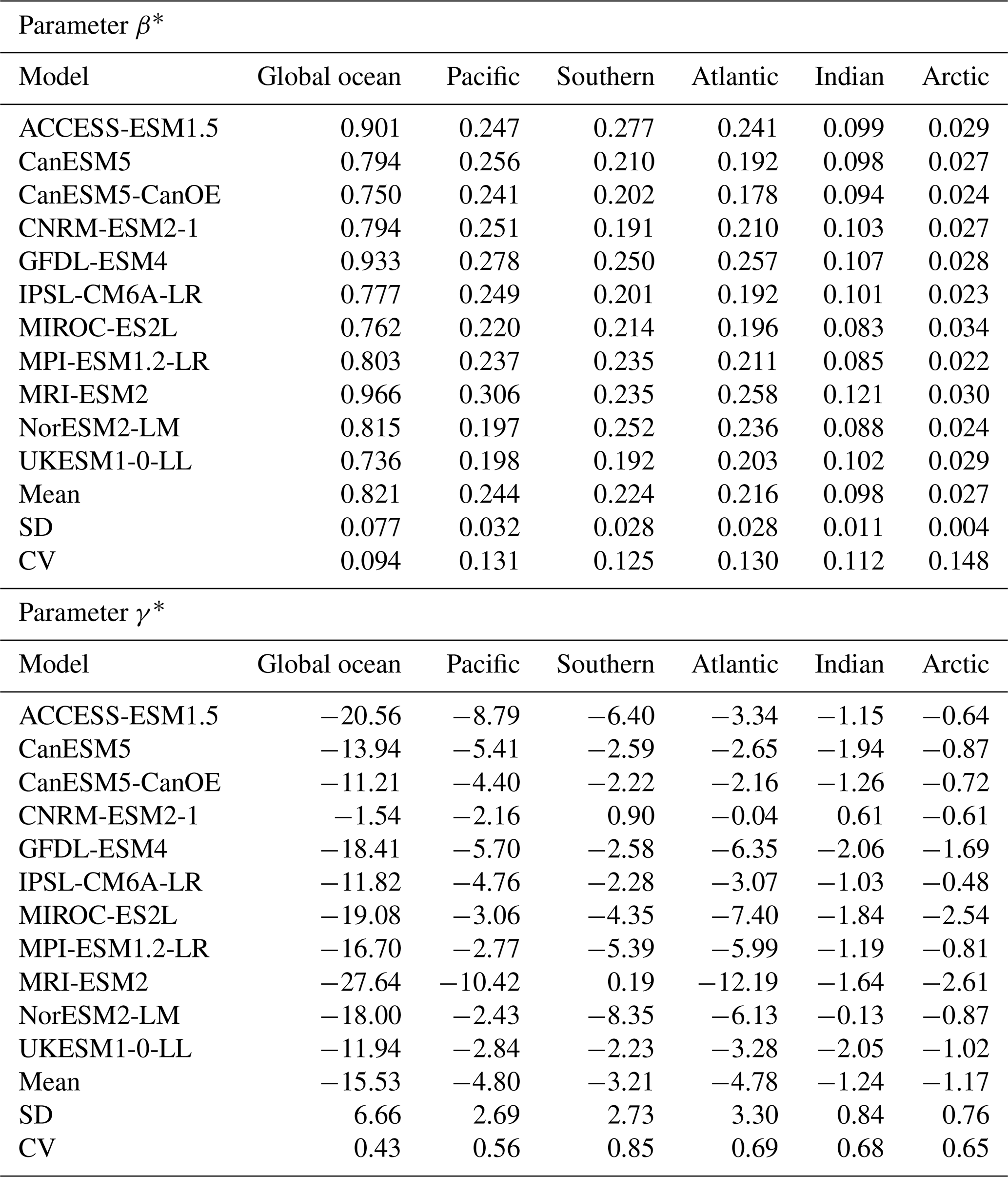
The ocean carbon–concentration feedback parameter, β, is positive in all the CMIP6 models (Table 2). The ocean carbon–climate feedback parameter, γ, is negative in all the Earth system models (Table 2), indicating that the ocean takes up less carbon in response to climate change. The variability in β amongst the Earth system models, as described by the coefficient of variation, CV, is relatively small on the global scale (CV = 0.09) when compared with the variability in γ (CV = 0.43) (Table 2). However, for the uncertainty in the ocean carbon gain due to carbon emissions, the carbon–concentration feedback contributes to a spread of 62 PgC, while the carbon–climate feedback contributes only to a spread of 25 PgC amongst the CMIP6 Earth system models on a global scale and to a quadrupling of atmospheric CO2, where the spread corresponds to 1 standard deviation.
Table 2Carbon–concentration feedback parameter based on carbon storage, β* (PgC ppm−1), and carbon–climate feedback parameter based on carbon storage, γ* (PgC K−1), for the global ocean and different ocean basins in 11 CMIP6 Earth system models, along with the inter-model mean; standard deviation; and coefficient of variation (CV), estimated as the standard deviation divided by the mean. The estimates are based on the fully coupled simulation (COU) and the biogeochemically coupled simulation (BGC) under the 1 % yr−1 increasing CO2 experiment. Diagnostics are from years 121 to 140 (the 20 years up to quadrupling of atmospheric CO2). Note that for the global ocean, β* and γ* are equivalent to β and γ.
2.2 Regional ocean
The carbon cycle feedbacks for the global ocean in Eq. (4) can be further separated into contributions from different ocean regions such that
where n denotes the different ocean regions; ΔCO2 and ΔT are the global changes in atmospheric CO2 and the surface air temperature, respectively; and βn, γn and 𝒩n are the carbon cycle feedback parameters and their non-linearity for each ocean region n.
Traditionally, the carbon cycle feedbacks are defined based on the cumulative carbon uptake from the atmosphere, Δ𝒮 (Tjiputra et al., 2010; Roy et al., 2011) such that the carbon cycle feedback parameters for each ocean region n are expressed as
where the carbon–climate feedback parameter, γn, corresponds to the effect of climate change under rising atmospheric CO2 and hence includes the effect of the non-linearity, 𝒩nΔCO2, in Eq. (6).
Alternatively, the carbon cycle feedbacks can be defined based on the carbon storage, such that the regional carbon cycle feedback parameters for each ocean region n are expressed as
where ΔIn is the change in the carbon inventory in region n. The carbon storage includes the combined effect from the local air–sea carbon exchange and the transport of carbon by the ocean circulation, such that
where Δ𝒮n is the regional cumulative ocean carbon uptake from the atmosphere relative to the pre-industrial era, and Δ𝒢n is the regional cumulative carbon gain relative to the pre-industrial era due to the ocean transport.
By substituting Eqs. (9) and (7) in Eq. (8) the two definitions for the carbon cycle feedback parameters are related by
Eq. (10) shows that the feedback parameters defined by the regional carbon storage, β* and γ*, are proportional to the feedback parameters defined by the regional cumulative carbon uptake, γ and β, but further modified by the ocean carbon transport.
2.2.1 Estimates based on carbon storage versus carbon uptake
On a global scale, the transport effect on the carbon storage integrates to zero, , such that the feedback parameters estimated from the carbon storage, β* and γ*, are equivalent to the feedback parameters estimated from the cumulative carbon uptake, β and γ, when ignoring the small carbon exchange between land and ocean. However, on regional scales the effect of the ocean transport on carbon storage leads to different spatial patterns in these carbon cycle feedback parameters, β and β* and γ and γ* (Fig. 2).
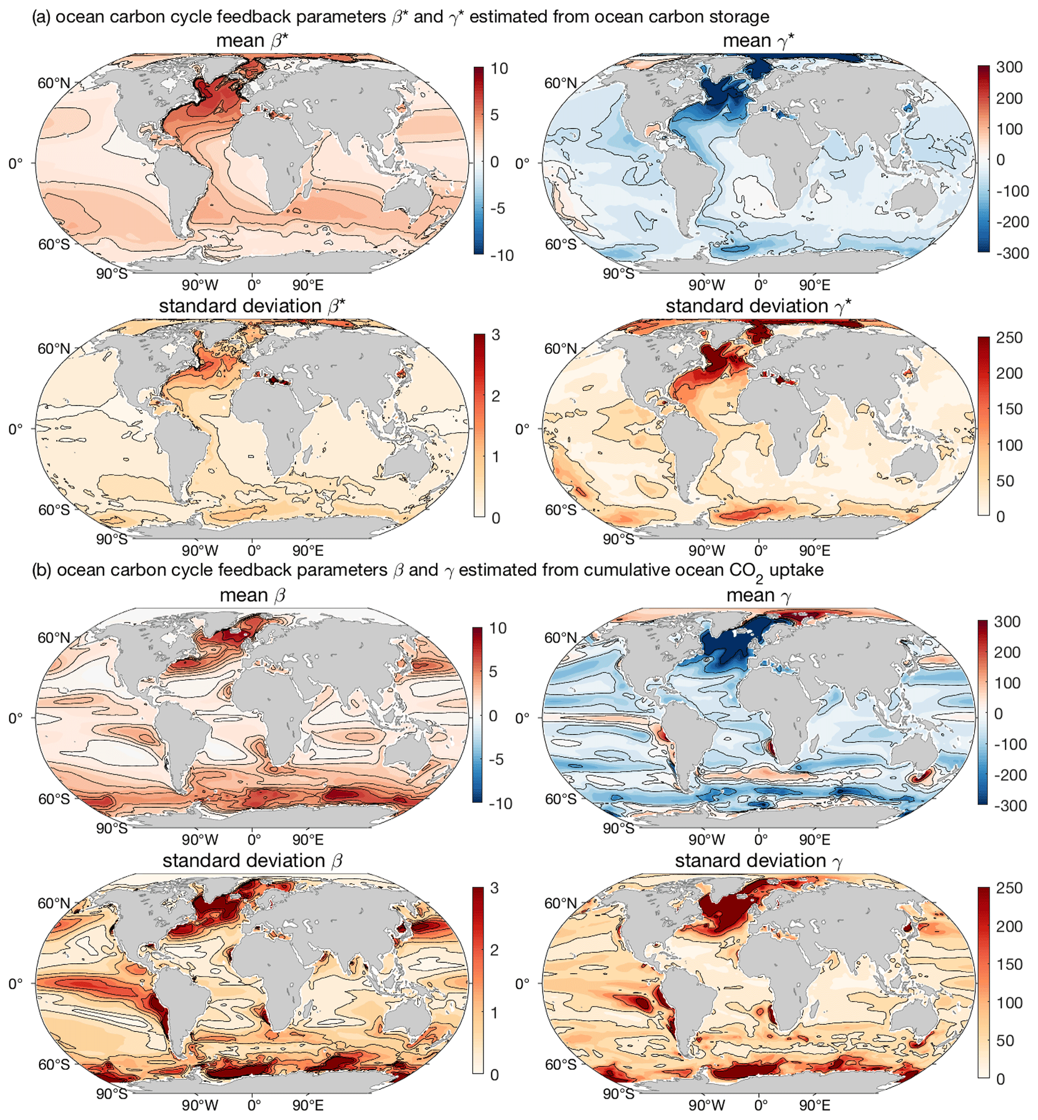
Figure 2Geographical distribution of the carbon cycle feedback parameters normalised by area: (a) β* (gC ppm−1 m−2) and γ* (gC K−1 m−2), estimated based on the regional ocean carbon storage, and (b) β (gC ppm−1 m−2) and γ (gC K−1 m−2), estimated based on the regional cumulative ocean carbon uptake. Results are shown as the inter-model mean and standard deviation based on 11 CMIP6 Earth system models (Table 1). The estimates are based on the fully coupled simulation (COU) and the biogeochemically coupled simulation (BGC) under the 1 % yr−1 increasing CO2 experiment. Diagnostics are from years 121 to 140 (the 20 years up to quadrupling of atmospheric CO2).
The carbon–concentration feedback parameter estimated from the cumulative carbon uptake, β, is largest and has more inter-model variability in (i) the Southern Ocean, (ii) the eastern boundary upwelling regions, (iii) the Gulf Stream and its extension into the North Atlantic Current, and (iv) the Kuroshio Extension (Fig. 2b). The inter-model variability in β is also significant along the equatorial Pacific, with this variability related to the inter-model spread in the trade winds and equatorial upwelling. In contrast, in the subtropical gyres, the ocean anthropogenic carbon uptake is limited and β is small (Fig. 2b).
The carbon–concentration feedback parameter estimated from ocean carbon storage, β*, is again large in the North Atlantic but instead large in the Southern Hemisphere subtropical gyres and small in the Southern Ocean south of 50∘ S relative to β (Fig. 2a). This difference between β and β* (Supplement Fig. S2) is due to the northward transport of anthropogenic carbon from the Southern Ocean associated with subduction and transport of mode and intermediate waters. The variability in β* amongst the models is large in the North Atlantic and extends south along the Atlantic western boundary (Fig. 2a).
The carbon–climate feedback parameter estimated from the cumulative carbon uptake, γ, is large and negative in the North Atlantic and in the Southern Ocean from 50 to 65∘ S (Fig. 2b). In contrast, γ is large and positive in a narrow band between 40 and 45∘ S, in the Southern Hemisphere eastern boundary upwelling regions, and in polar regions with sea ice. The regions of large ocean carbon loss or uptake from the atmosphere due to climate change, as shown by the large γ, also experience the largest variability in γ amongst the CMIP6 Earth system models (Fig. 2b).
The effect of carbon transport on γ* is of opposite sign to the effect of the cumulative carbon uptake in most regions (Supplement Fig. S2). This transport effect leads to a γ* that is overall less negative in the Southern Ocean and in the high latitudes of the North Atlantic but more negative in the Arctic, the equatorial Pacific and along the Atlantic western boundary relative to γ (Fig. 2a). The spread in γ* amongst the models is largest in the North Atlantic, in the Arctic, along the Atlantic western boundary and in the Southern Ocean (Fig. 2a).
The carbon cycle feedbacks estimated from the cumulative carbon uptake better describe the atmosphere–ocean interaction. The carbon cycle feedbacks estimated from the ocean carbon storage instead better describe the response of the ocean carbon budget to carbon emissions. Here, we focus on the carbon cycle feedbacks estimated from the regional ocean carbon storage to enable diagnostics in terms of the preformed and regenerated carbon pools and to gain more mechanistic insight.
2.2.2 Basin-scale β* and γ*
We define the Southern Ocean as south of 35∘ S and the Arctic Ocean as north of 65∘ N, and we exclude semi-enclosed seas from our basins' definition (see Supplement Fig. S1 for a map of the regions). The Pacific, Southern and Atlantic oceans contribute equally to the ocean carbon–concentration feedback parameter, as estimated in terms of carbon storage, with an inter-model mean β* of 0.24, 0.22 and 0.22 PgC ppm−1, respectively (Table 2). The Indian Ocean contributes less than half than the other three basins to β*, with an inter-model mean of 0.10 PgC ppm−1 (Table 2). The Arctic Ocean has a β* of only 0.03 PgC ppm−1. The Pacific, Southern, Atlantic, Indian and Arctic oceans have an inter-model mean carbon–climate feedback parameter, defined in terms of carbon storage, γ*, of −4.8, −3.2, −4.8, −1.2 and −1.2 PgC K−1, respectively (Table 2). The basin-scale variability in β* amongst the models, as described by the coefficient of variation, CV, is less than 0.15 (Table 2). The basin-scale variability in γ* amongst the models varies from CV = 0.56 in the Pacific Ocean to CV = 0.85 in the Southern Ocean (Table 2). The inter-model variability in β* and γ* for each basin is larger than that of the global ocean (Table 2), which suggests that variability in different basins compensate for each other. For diagnostics of the separate contribution of the ocean carbon uptake and transport on the basin-scale carbon storage and for feedback parameters see Appendix A.
To gain insight into the driving mechanisms of the carbon cycle feedbacks and their uncertainty amongst Earth system models, β* and γ* may be separated into contribution from the regenerated, the saturated and the disequilibrium ocean carbon pools following the methodology of Williams et al. (2019) and Arora et al. (2020). The ocean dissolved inorganic carbon, DIC, may be defined in terms of these separate carbon pools (Ito and Follows, 2005; Williams and Follows, 2011; Lauderdale et al., 2013; Bernardello et al., 2014):
where DICpref is the part of the DIC transferred from the surface into the ocean interior due to the physical ventilation, involving the circulation, and DICreg is the part of the DIC accumulated into the ocean interior due to biological regeneration of organic carbon. Similarly, the DICpre can be viewed as the part of the DIC associated with the solubility pump and the DICreg as the part of the DIC associated with the biological pump. The DICpref can be further split into two idealised carbon pools: (i) the DICsat representing the amount of DIC that the ocean would have if the whole ocean reached a full chemical equilibrium with the contemporaneous atmospheric CO2 concentration and (ii) the DICdis representing the extent that the ocean departs from a full chemical equilibrium with the contemporaneous atmospheric CO2. Assuming the changes in the biological organic carbon inventory are small, the changes in the ocean carbon inventory relative to the pre-industrial era, ΔIocean in petagrams of carbon, are related to the volume integral of the changes in each of the DIC pools, ΔDIC in moles per cubic metre, as
where PgC mol−1 is a unit conversion from moles to petagrams of carbon.
By substituting Eq. (12) into Eq. (5), for the global ocean, or into Eq. (8), for the regional ocean, the carbon cycle feedback parameters may be diagnosed in terms of these different ocean carbon pools (Williams et al., 2019; Arora et al., 2020):
3.1 Contribution from the saturated carbon pool to β* and γ*
The saturated part of β* and γ* in Eq. (13) is expressed as
The changes in the saturated carbon pool relative to the pre-industrial era in Eq. (14) are diagnosed as
where Δ is the change relative to the pre-industrial era, Tocean is the ocean temperature, S is the ocean salinity, P is the ocean phosphate concentration, Si is the ocean silicate concentration, Alkpre is the preformed alkalinity and f is a non-linear function representing the solution to the ocean carbonate chemistry which provides DICsat for the contemporaneous atmospheric CO2. Here, f is estimated following the iterative solution for the ocean carbonate chemistry of Follows et al. (2006) and by considering the small contribution of minor species (borate, phosphate, silicate) to the preformed alkalinity. In the limit that the ocean hydrogen ion concentration at a chemical equilibrium with the given atmospheric CO2, [H+]sat, is known or the preformed alkalinity is assumed equal to the carbonate alkalinity, the f function corresponds to the usual solution of the carbonate system that provides DICsat based on two knowns: atmospheric CO2 and either [H+]sat (see Eq. 18) or carbonate alkalinity. The preformed alkalinity is estimated from a multiple linear regression using salinity and the conservative tracer PO (Gruber et al., 1996), with the coefficients of this regression estimated based on the surface (first 10 m) alkalinity, salinity, oxygen and phosphate in each of the Earth system models.
To understand how the ocean carbonate chemistry operates and the mechanisms that control βsat, consider an ocean buffer factor, B, where the fractional change in the atmospheric CO2 and saturated carbon inventory is defined relative to the pre-industrial era (Katavouta et al., 2018):
where subscript 0 denotes the pre-industrial era.
Substituting Eq. (16) into Eq. (14) the saturated part of β* can be expressed as
where is the ocean buffer factor for the increasing atmospheric CO2 but with no climate change (i.e. for the pre-industrial ocean temperature, salinity and alkalinity), as is the case in the BGC run.
Eq. (17) shows that βsat is proportional to the ocean capacity to buffer changes in atmospheric CO2 with no changes in the physical climate, . The rise in atmospheric CO2 leads not only to an increase in the saturated ocean carbon inventory, ΔIsat (Fig. 3a, red shade), but also to a decrease in the ocean capacity to buffer changes in atmospheric CO2 as the ocean acidifies. Accordingly, the buffer factor, B, increases and βsat decreases with the rise in atmospheric CO2 at a global and basin scale in all the Earth system models (Fig. 3b, red shade). The buffer factor, B, and thus βsat also depend on the pre-industrial ocean state due to the non-linearity of the ocean carbonate system. Hence, there is a spread in βsat amongst the Earth system models forced by the same increase in atmospheric CO2 (Fig. 3b, red shade) related to their different pre-industrial ocean temperature, salinity and alkalinity.
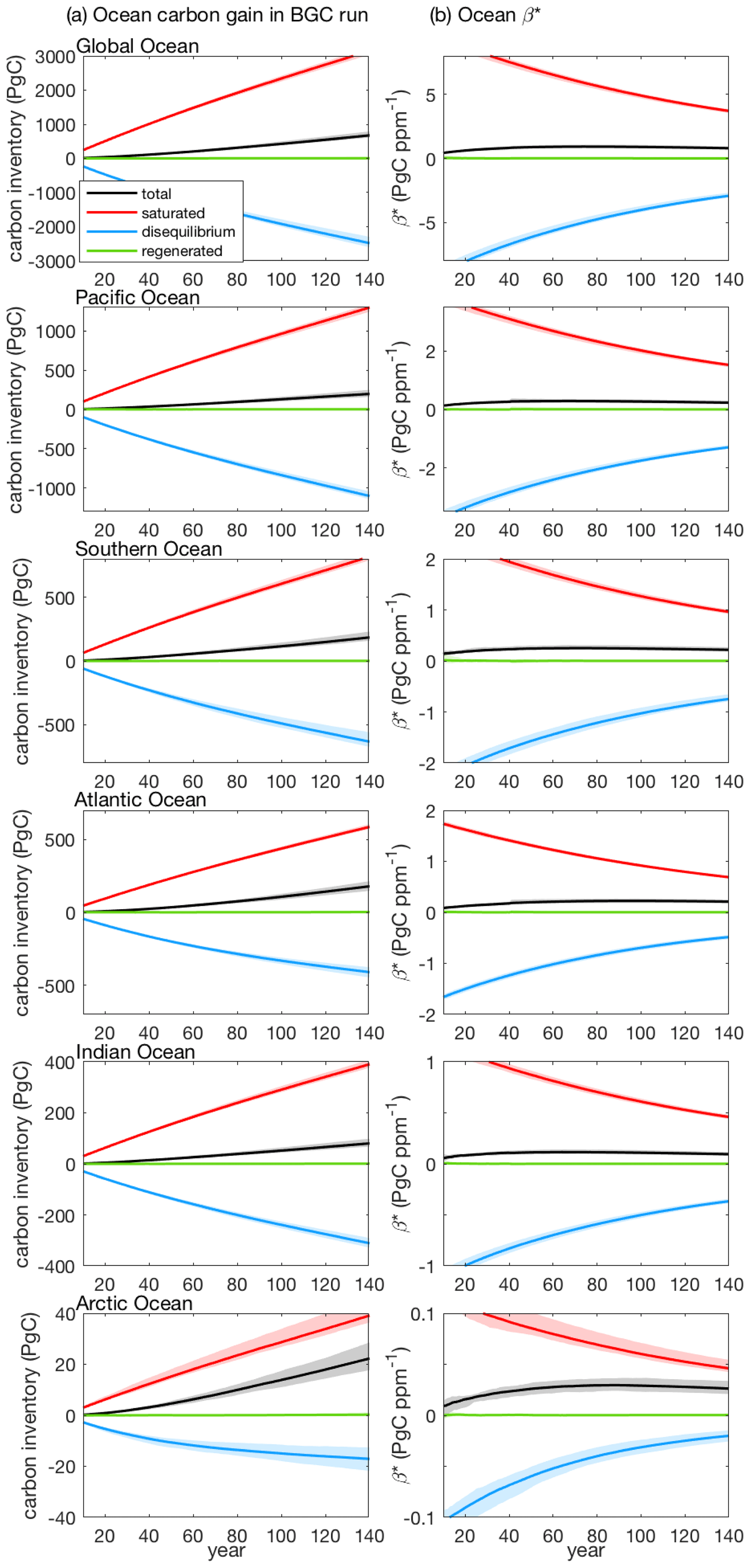
Figure 3Ocean carbon storage and ocean carbon–concentration feedback parameter, β*, for the global ocean and different ocean basins, along with the contribution from the saturated, disequilibrium and regenerated carbon pools in CMIP6 Earth system models: (a) ocean carbon inventory changes relative to the pre-industrial era in the biogeochemically coupled simulation (BGC) and (b) ocean carbon–concentration feedback parameter based on carbon storage, β* (PgC ppm−1). The solid lines and the shading show the model mean and the model range, respectively, based on the 1 % yr−1 increasing CO2 experiment over 140 years in 11 CMIP6 models (Table 1). Note that for the global ocean, β* is equivalent to β.
To understand the mechanisms that control γsat, consider the solution to the saturated part of DIC as dictated by the carbonate chemistry,
where
Ko is the solubility, K1 and K2 are the ocean carbon dissociation constants, and [H+]sat is the ocean hydrogen ion concentration at a chemical equilibrium with the contemporaneous atmospheric CO2. Ko, K1 and K2 are a function of the ocean temperature and salinity and so depend on the physical climate change, while [H+]sat depends primarily on the changes in atmospheric CO2. Combining Eq. (18) with Eqs. (14) and (15) and assuming that the ocean temperature and salinity remain at their pre-industrial value in the BGC run with no climate change, γsat can be expressed as
By expanding , Eq. (19) can be written as
The first term in curly brackets in Eq. (20) contributes to the linear part of γsat and is controlled by changes in climate only, specifically by the effect of changes in the ocean temperature to the solubility and ocean carbon dissociation constants. Under warming due to changes in climate, this term is negative. The second term in curly brackets in Eq. (20) contributes to the non-linear part of γsat, and it depends on changes in pH, due to the increase in atmospheric CO2, and changes in climate. Under rising atmospheric CO2 and warming, this term is negative as [H+]sat increases and Ko decreases, and it is smaller than the linear term as . The adjustment of γsat due to changes in the pH, represented by this non-linear term, depends on the increase in atmospheric CO2; for example, the non-linear term is about 30 % and 50 % of the linear term for a doubling of atmospheric CO2 and for a quadrupling of atmospheric CO2, respectively. Hence, the non-linearity of the carbonate chemistry acts to reduce the magnitude of the negative γsat consistent with the carbonate system being less sensitive to change in temperature under higher ocean DIC (Schwinger et al., 2014).
Eq. (20) shows that γsat is proportional to the changes in solubility due to climate change and is further modified by changes in the ocean carbon dissociation constants with warming and by the non-linearity of the carbonate chemistry. Ocean warming due to climate change leads to a decrease in the saturated carbon inventory, ΔIsat, in all basins (Fig. 4a, red shade) primarily driven by a decrease in solubility. This decrease in ΔIsat with warming drives a nearly constant negative γsat (Fig. 4b, red shade) with the deviations from a constant value being associated with the non-linearity of the carbonate system. The spread of γsat amongst the Earth system models (Fig. 4b, red shade) is relatively small at a global and basin scale, except in the Arctic, and is associated with different pre-industrial ocean states in the models.
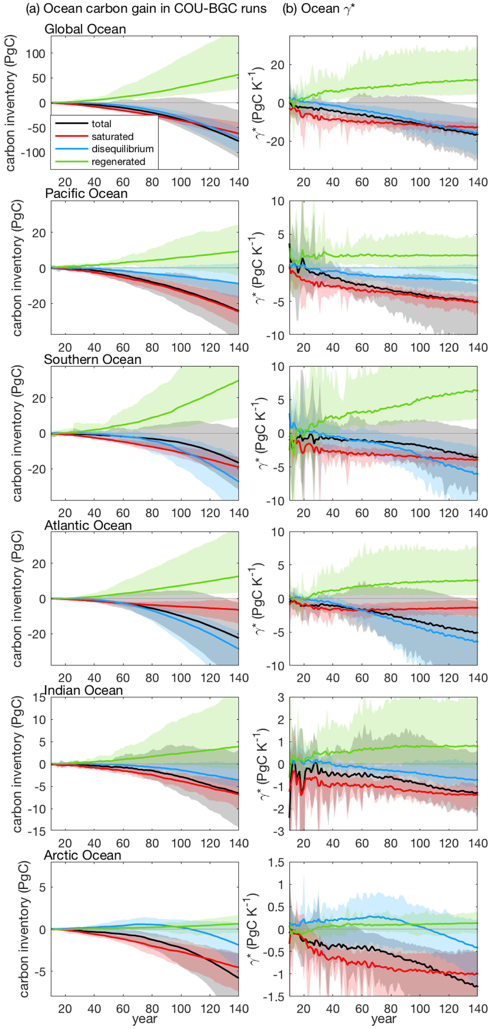
Figure 4Ocean carbon storage and ocean carbon–climate feedback parameter, γ*, for the global ocean and different ocean basins, along with the contribution from the saturated, disequilibrium and regenerated carbon pools in CMIP6 Earth system models: (a) ocean carbon inventory changes in the fully coupled simulation (COU) minus the biogeochemically coupled simulation (BGC) and (b) ocean carbon–climate feedback parameter based on carbon storage, γ* (PgC K−1). The solid lines and the shading show the model mean and the model range, respectively, based on the 1 % yr−1 increasing CO2 experiment over 140 years in 11 CMIP6 models (Table 1). Note that for the global ocean, γ* is equivalent to γ.
3.2 Contribution from the regenerated carbon pool to β* and γ*
The regenerated part of β* and γ* in Eq. (13) is expressed as
Assuming that the oxygen concentration is close to saturation at the surface, DICreg can be estimated from the apparent oxygen utilisation, AOU, and the contribution of biological calcification to alkalinity, Alk (Ito and Follows, 2005; Williams and Follows, 2011; Lauderdale et al., 2013), such that ΔIreg in Eq. (21) is diagnosed as
where RCO and RNO are constant stoichiometric ratios and Alkpre is the preformed alkalinity such that Alk−Alkpre gives the contribution to alkalinity from biological calcification.
The regenerated part of β* is associated with changes in ocean biological processes due to the atmospheric CO2 increase. and βreg are effectively negligible in the Earth system models (Fig. 3a and b, green shade) as these models do not include an explicit dependence of biological production on an increase in carbon availability or decrease in seawater pH. The regenerated part of γ* is associated with changes in ocean biological processes due to changes in climate, including the effect of changes in the circulation on the sinking rate of particles, the effect of warming on the solubility of oxygen and the effect of changes in alkalinity on the dissolution of the calcium carbonate shells of calcifying phytoplankton. and γreg are positive and increase in time on a global and basin scale (Fig. 4a and b, green shade), indicating that γreg is dominated by the weakening in the ocean physical ventilation due to climate change. This weakening in the ocean physical ventilation leads to a longer residence time of water masses in the ocean interior and so to an increase in the accumulation of carbon from the regeneration of biologically cycled carbon in the deep ocean (Schwinger et al., 2014; Bernardello et al., 2014).
3.3 Contribution from the disequilibrium carbon pool to β* and γ*
The disequilibrium parts of β* and γ* are diagnosed using Eq. (13) as
The disequilibrium part of the carbon cycle feedback parameters is controlled by the ocean physical ventilation. Specifically, βdis is a function of the pre-industrial ocean physical ventilation and the rate of transfer of the anthropogenic carbon from the ocean surface into the ocean interior. The rise in atmospheric CO2 leads to an increase in the magnitude of the negative disequilibrium ocean carbon inventory, ΔIdis, at a global and basin scale (Fig. 3a, blue shade), as the ocean physical ventilation is relatively slow and the ocean carbon transfer over the ocean interior cannot keep up with the rate of increase in atmospheric CO2. Hence, βdis is negative at a global and basin scale in all the Earth system models (Fig. 3b, blue shade). However, the rate of increase in the magnitude of ΔIdis slows down in time (Fig. 3a, blue shade) and βdis becomes less negative in time (Fig. 3b, blue shade), as more anthropogenic carbon is transferred into the ocean interior while the buffer capacity of the ocean decreases, which brings the ocean closer to an equilibrium with the contemporaneous atmospheric CO2.
The disequilibrium part of γ* depends on the weakening of the ocean physical ventilation with climate change. Here, γdis is defined based on the climate change impact under rising atmospheric CO2 (i.e. COU–BGC runs) and so includes (i) the effect of weakening ventilation on the pre-industrial ocean carbon gradient involving the natural carbon, (ii) the effect of weakening ventilation on the anthropogenic carbon, and (iii) the effect from decreasing sea-ice coverage leading to an increase in the ocean in direct contact with the atmosphere. Overall, the effect of the weakening ventilation on the combined anthropogenic and natural carbon leads to a negative ΔIdis and a negative γdis on a global scale and in the Atlantic, Indian, Pacific and Southern oceans after year 40 (Fig. 4a and b, blue shade). In the Arctic, the effect of the decreasing sea-ice coverage drives a slightly positive γdis over the first 80 years, while the effect of the weakening ventilation dominates and drives a negative γdis after year 80. The disequilibrium part of γ* becomes more negative in time on a global and basin scale as the ocean ventilation weakens with warming.
3.4 Combined effect of saturated, disequilibrium and regenerated carbon pools on β* and γ*
On a global and basin scale, the ocean carbon–concentration feedback parameter, β*, is positive in all the Earth system models. This positive β* is explained by the chemical response involving the rise in ocean saturation, βsat, opposed by the effect of the relatively slow ocean ventilation, such that the physical uptake of carbon within the ocean is unable to keep pace with the rise in atmospheric CO2, βdis (Fig. 3b). There is no significant contribution from biological changes to β* in the Earth system models. The spread in βsat amongst the Earth system models is small on a global and basin scale (Fig. 5a), reflecting the use of similar carbonate chemistry schemes and bulk parameterisations of air–sea CO2 fluxes across marine biogeochemical models in CMIP6 (Séférian et al., 2020). The spread in βdis is also small on a global and basin scale (Fig. 5a) as all the Earth system models have a broadly similar general circulation and physical ventilation in the pre-industrial era.
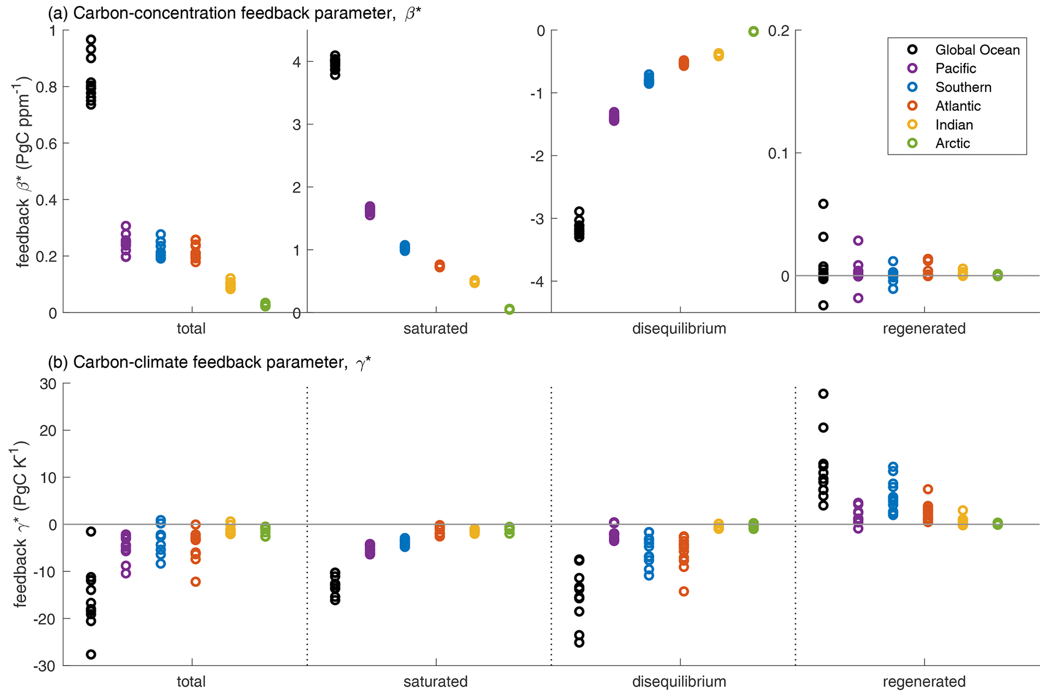
Figure 5Carbon cycle feedback parameters based on carbon storage, along with the contribution from the saturated, disequilibrium and regenerated carbon pools, for the global ocean and the different ocean basins in 11 CMIP6 Earth system models (Table 1): (a) carbon–concentration feedback parameter, β* (PgC ppm−1), and (b) carbon–climate feedback parameter, γ* (PgC K−1). The estimates are based on the fully coupled simulation (COU) and the biogeochemically coupled simulation (BGC) under the 1 % yr−1 increasing CO2 experiment. Diagnostics are from years 121 to 140 (the 20 years up to quadrupling of atmospheric CO2). For the inter-model mean and standard deviation of these estimates, see Supplement Table S1. Note that for the global ocean, β* and γ* are equivalent to β and γ.
The decrease in solubility and in the physical ventilation with warming reduces the ocean carbon uptake, leading to negative γsat and γdis, respectively (Fig. 4b). However, the decrease in the ventilation with warming also acts to increase the residence time in the ocean interior, leading to an increase in the regenerated carbon and a positive γreg (Fig. 4b, green shading). The combined γsat and γdis dominate over the opposing γreg, leading to an overall negative γ* on a global and basin scale. On a global scale, γsat, γdis and γreg are of a similar magnitude (Fig. 5b, black circles). The inter-model spread in the global γ* is mainly driven by the spread in γdis and γreg (Fig. 5b, black circles) and is associated with the different response of the ocean ventilation to warming in these models. The inter-model spread in the global γreg is larger than the spread in the global γdis due to the different parameterisations of ocean biogeochemical processes in the models.
In the Southern Ocean, the contributions from the saturated, disequilibrium and regenerated carbon pools to γ* are of a similar magnitude (Fig. 5b, blue circles), such that the decrease in solubility, the reduction in the physical ventilation and the increase in the regenerated carbon accumulation in the ocean interior due to climate change are equally important. The inter-model spread in γ* in the Southern Ocean is dominated by the spread in γdis and γreg. In the Pacific and Indian oceans, the magnitude of γ* is primarily controlled by the saturated carbon pool and the decrease in carbon solubility due to warming (Fig. 5b, purple and yellow circles). However, the inter-model spread in γ* in the Pacific and Indian oceans is dominated by the response of the regenerated carbon pool to climate change, γreg (Fig. 5b, purple and yellow circles). In the Atlantic Ocean, γ* is dominated by the disequilibrium carbon pool (Fig. 5b, red circles) and the reduction in the physical ventilation due to climate change, with the contribution from the saturated carbon pool being relatively small. In the Arctic Ocean, γ* is primarily controlled by the saturated carbon pool and the decrease in solubility, with the contribution from the regenerated carbon pool being negligible (Fig. 5b, green circles).
On regional scales, the contributions from the saturated, disequilibrium and regenerated carbon pools to β* and γ* are further modified by local upwelling, changes in alkalinity and the conversion of regenerated carbon to disequilibrium carbon at the ocean surface, as discussed in Appendix B.
3.5 Processes controlling the contribution from different basins to β* and γ*
The Southern and Indian oceans contribute 27 % and 12 %, respectively, to the ocean carbon–concentration feedback parameter, β*, following their fractional volumes of the global ocean (Fig. 6a). However, the Atlantic and Arctic oceans contribute 26 % and 3 % to β*, respectively, which is significantly more than their fractional volume of 18 % and 1 % of the global ocean. In contrast, the Pacific Ocean contributes only 30 % to β* despite its fractional volume of 42 % of the global ocean. By definition, the contribution of each basin to βsat is approximately proportional to the ocean volume contained in each basin (Fig. 6a). However, βdis is relatively low in the Atlantic and Arctic oceans and high in the Pacific Ocean compared with their respective volumes (Fig. 6a), which may be understood by the Atlantic and Arctic oceans interior being more ventilated and the Pacific Ocean interior being less ventilated than the rest of the ocean. Specifically, the low βdis and the relatively large contribution from the Atlantic Ocean to β* are due to a large transfer of anthropogenic carbon into the ocean interior from strong local physical ventilation and transport of carbon from the Southern Ocean. In the Arctic Ocean, the transfer of anthropogenic carbon from the well-ventilated Atlantic Ocean contributes towards a decrease in βdis and to a relatively large β*. The Southern Ocean has large anthropogenic carbon uptake from the atmosphere, but its contribution to β*, as estimated from carbon storage, is relatively small due to large carbon transport to the other basins (Fig. A1).
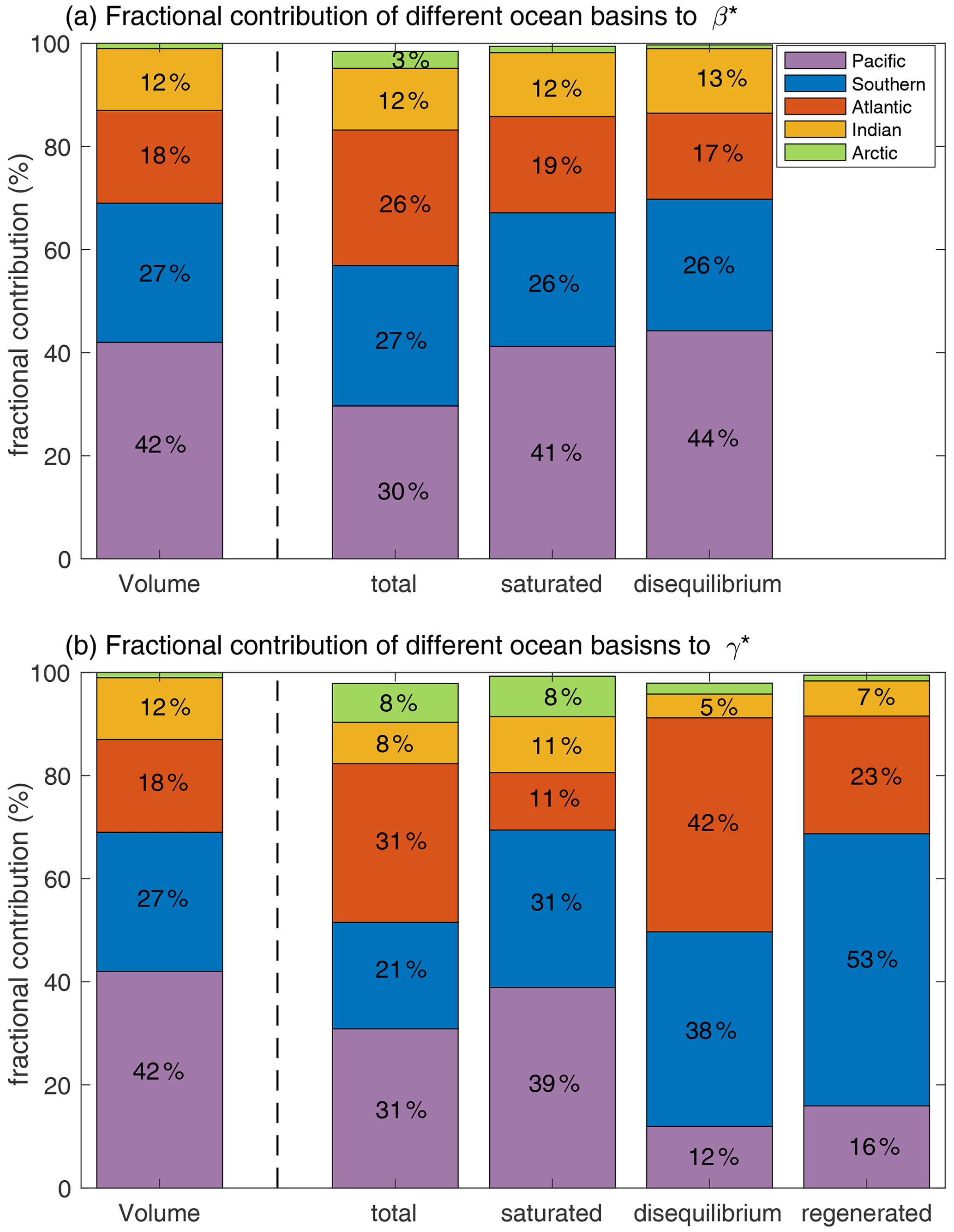
Figure 6The fractional contribution (in %) of different ocean basins to the total volume of the ocean and to the ocean carbon cycle feedback parameters based on carbon storage, along with the contribution from the saturated, disequilibrium and regenerated carbon pools based on the inter-model mean of 11 CMIP6 models (Table 1): (a) carbon–concentration feedback parameter, β*, and (b) carbon–climate feedback parameter, γ*. The estimates are based on the fully coupled simulation (COU) and the biogeochemically coupled simulation (BGC) under the 1 % yr−1 increasing CO2 experiment. Diagnostics are from years 121 to 140 (the 20 years up to quadrupling of atmospheric CO2). The regenerated part of β* is omitted as its contribution is negligible in all basins (Fig. 5a). The Arctic Ocean has a fractional volume of ∼ 1 % of the global ocean and a fractional contribution of 1.2 %, 0.7 %, 2 % and 1 % to βsat, βdis, γdis and γreg, respectively (not explicitly shown in the figure). The combined fractional contribution of the five ocean basins to β* and γ* is less than 100 % due to a small contribution, <2 %, from semi-enclosed seas with a fractional volume of less than 0.5 % of the global ocean (Supplement Fig. S1).
The Pacific and Indian oceans' contributions to γsat are slightly smaller than expected from their fractional volumes (Fig. 6b), consistent with a low warming per unit volume in these basins (Fig. 1d). The Pacific and Indian oceans' contributions to γdis and γreg are significantly smaller than expected from their fractional volumes (Fig. 6b), indicating that there is no significant effect from changes in ventilation in these basins. This absence of any significant effect from changes in the ventilation with warming in the Pacific and the Indian oceans leads to their much smaller contribution to γ* relative to their volumes (Fig. 6b).
The Atlantic Ocean has a contribution of 31 % to γ*, which is much larger than expected from its fractional volume of 18 % of the global ocean. This large contribution from the Atlantic Ocean is primarily due to γdis (Fig. 6b) and the reduction in the physical ventilation due to climate change. The Atlantic Ocean has a smaller contribution to γsat than expected from its fractional volume (Fig. 6b), despite experiencing large warming (Fig. 1d), which suggests that the non-linearity of the carbonate system is important in this basin. Specifically, the Atlantic Ocean has a large increase in DIC (Fig. 1c) which acts to significantly reduce the magnitude of the negative γsat driven solely by the effect of warming on solubility (see Eq. 20). The Arctic Ocean has a contribution of 8 % to γ*, which is much larger than expected from its fractional volume of 1 % of the global ocean. This large contribution from the Arctic Ocean is primarily associated with the saturated part of γ* (Fig. 6b) and a very large warming per unit volume in this basin (Fig. 1d).
The Southern Ocean has a contribution of 38 % to γdis and of 53 % to γreg, which is much larger than expected from its fractional volume (Fig. 6b). These large contributions indicate that changes in the physical ventilation and the accumulation of regenerated carbon due to climate change have a large effect on the Southern Ocean carbon storage. The Southern Ocean contribution to γsat is also larger than expected from its fractional volume (Fig. 6b), consistent with a large warming per unit volume in this basin (Fig. 1d). Hence, the apparent small contribution of the Southern Ocean to γ*, of 21 %, is due to compensation between (i) the large decrease in carbon storage associated with the combined decrease in solubility and physical ventilation and (ii) the large increase in carbon storage associated with a longer residence time and accumulation of regenerated carbon in the Southern Ocean interior.
The ocean carbon cycle feedbacks are controlled by ocean ventilation and the transfer of carbon from the mixed layer to the thermocline and deep ocean. The ocean ventilation involves the seasonal cycle of the mixed layer; the subduction process; and the effects of the eddy, gyre and overturning circulations. Despite this complexity, the strength of the Atlantic Meridional Overturning Circulation (AMOC) and its weakening due to climate change is often used as a proxy for the large-scale ocean ventilation. Here we investigate the dependence of the carbon cycle feedbacks on the AMOC strength and its weakening with climate change.
4.1 Insight from an idealised climate model with a meridional overturning
The idealised climate model of Katavouta et al. (2019) is used to investigate the control of the carbon cycle feedbacks by the AMOC. This idealised model consists of a slab atmosphere, two upper ocean boxes for the southern and northern high latitudes, two boxes for the mixed layer and the thermocline in the low and middle latitudes, and one box for the deep ocean (Fig. 7a). The model solves for the thermocline thickness from a volumetric balance between the surface cooling conversion of light to dense waters in the North Atlantic, the diapycnal transfer of dense to light waters in low and middle latitudes, and the conversion of dense to light waters in the Southern Ocean involving Ekman transport partially compensated for by poleward mesoscale eddy transport (Gnanadesikan, 1999; Johnson et al., 2007; Marshall and Zanna, 2014). The model also accounts for the rate of subduction occurring in the Southern Ocean versus the tropics and subtropics through an isolation fraction for water remaining below the mixed layer and spreading northwards in the thermocline. The model solves for the ocean carbon cycle including physical and chemical transfers but ignores biological transfers and sediment and weathering interactions involving changes in the cycling of organic carbon or calcium carbonate. The ocean carbonate system is solved using the iterative algorithm of Follows et al. (2006). For the model closures and an explicit description of the model budgets and equations, see Katavouta et al. (2019).
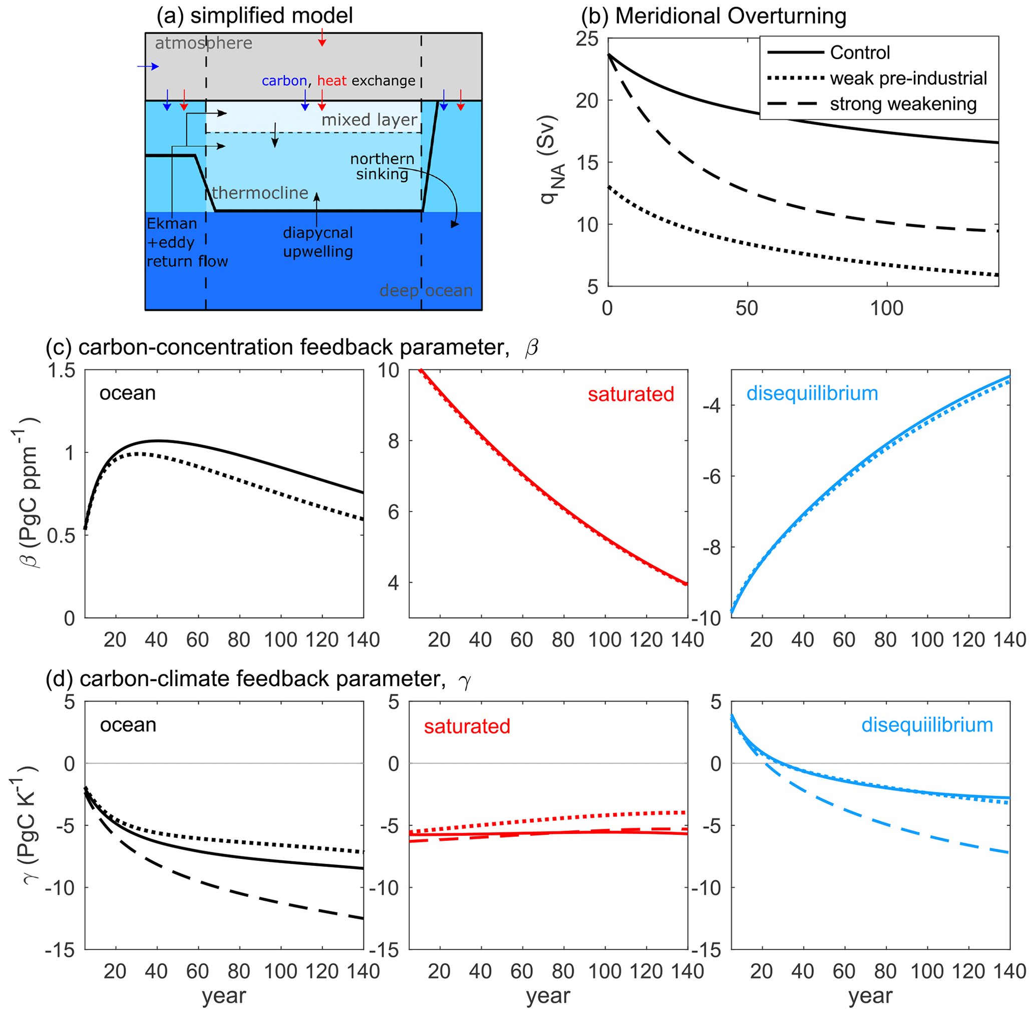
Figure 7(a) A simplified climate model with overturning circulation, including a slab atmosphere, an upper layer of light water consisting of a thermocline layer and a surface mixed layer in the low and middle latitudes, two upper layers at southern and northern high latitudes, and a lower layer of dense water. (b) Meridional overturning in the three experiments forced by a 1 % yr−1 increase in atmospheric CO2: (i) control experiment (solid line), (ii) weaker pre-industrial overturning (dotted line) and (iii) larger reduction in the overturning with climate change (dashed line). (c) The ocean carbon–concentration feedback parameter, β, and (d) the ocean carbon–climate feedback parameter, γ, along with their saturated and disequilibrium parts, in the experiments with different meridional overturning. The estimates of β and γ are based on the fully coupled simulations (COU) and the biogeochemically coupled simulations (BGC). Note that for the “global” ocean of the simplified model, β and γ are equivalent to β* and γ*.
The model is first integrated to a pre-industrial steady state, with the distribution of temperature and DIC depending on the pre-industrial strength of the overturning. The model is then forced by a 1 % yr−1 increase in atmospheric CO2 concentration from a pre-industrial value of 280 ppm until atmospheric CO2 quadruples over a 140-year period. This increase in atmospheric CO2 drives a radiative forcing: , where a is 5.35 W m−2 (Myhre et al., 1998) and subscript 0 denotes the pre-industrial state. This radiative forcing then drives a radiative response, λΔTair, and net planetary heat uptake given by the downward heat flux entering the system at the top of the atmosphere, NTOA (Gregory et al., 2004) such that , where Tair is the temperature of the slab atmosphere and λ is the climate feedback parameter that is assumed constant and equal to 1 W m−2 K−1 for simplicity. The ocean heat uptake, N, is estimated as the planetary heat uptake minus the atmospheric heat uptake, , where c=50 W m−2 K−1 is an air–sea heat transfer parameter and Tsurf is the ocean temperature at the surface. The ocean heat uptake is distributed equally over the ocean surface. For this model closure, the ocean heat uptake is more than 95 % of the net planetary heat uptake.
This additional ocean heat uptake reduces the conversion of light to dense waters in the North Atlantic, qNA, and leads to an overturning weakening, following
where A is the model area covered by the low and middle latitudes; ρ is a referenced ocean density; Cp is the specific heat capacity for the ocean; and Tcontrast is the temperature contrast between light waters in the low and middle latitudes, involving the mixed layer and thermocline, and the dense waters in the deep ocean.
Three experiments were conducted using this idealised model forced by a 1 % yr−1 increase in atmospheric CO2: (i) a control experiment with a strong pre-industrial AMOC that experiences a weakening with warming as described by Eq. (24) (solid line in Fig. 7b); (ii) an experiment with a weak pre-industrial AMOC that experiences the same weakening with warming as in the control experiment (dotted line in Fig. 7b); and (iii) an experiment with a strong pre-industrial AMOC that experiences a doubled weakening with warming compared to that in the control experiment, such that the right hand of Eq. (24) is multiplied by a factor of 2 (dashed line in Fig. 7b). In all the experiments, a fully coupled simulation (COU) and a biogeochemically coupled simulation (BGC) are used to estimate the carbon cycle feedback parameters β and γ.
In the idealised model, a weaker pre-industrial meridional overturning leads to a smaller carbon–concentration feedback parameter, β, during the centennial transient response to the increase in atmospheric CO2 (Fig. 7c, black lines). The saturated part of β does not directly depend on the AMOC strength (Fig. 7c, red lines). In contrast, a weaker pre-industrial AMOC leads to a more negative disequilibrium part of β (Fig. 7c, blue lines) due to a weaker and slower transfer of anthropogenic carbon below the ocean surface. Hence, the pre-industrial AMOC controls β through its effect on the physical ventilation via the disequilibrium carbon pool.
The strength of the pre-industrial meridional overturning has only a small impact on the carbon–climate feedback parameter, γ, that is associated with the saturated carbon pool (Fig. 7d, solid and dotted lines). In the idealised model, a different pre-industrial overturning is associated with a different pre-industrial ocean state, in terms of temperature and DIC, which has a small effect on the saturated part of γ due to the non-linearity of the carbonate chemistry. The carbon–climate feedback parameter, γ, is primarily controlled by the changes in the AMOC with warming and specifically by the dependence of the negative γdis on the AMOC weakening with warming (Fig. 7d, solid and dashed lines). Hence, a more pronounced weakening in the AMOC with warming drives a more negative γ, as there is a more pronounced decrease in the physical transfer of carbon into the ocean interior.

Figure 8The Atlantic Meridional Overturning Circulation (AMOC; in Sv), in the pre-industrial era: (a–k) 11 CMIP6 Earth system models and (l) their inter-model mean. The estimates are based on pre-industrial control simulation (piControl) for years 121 to 140.
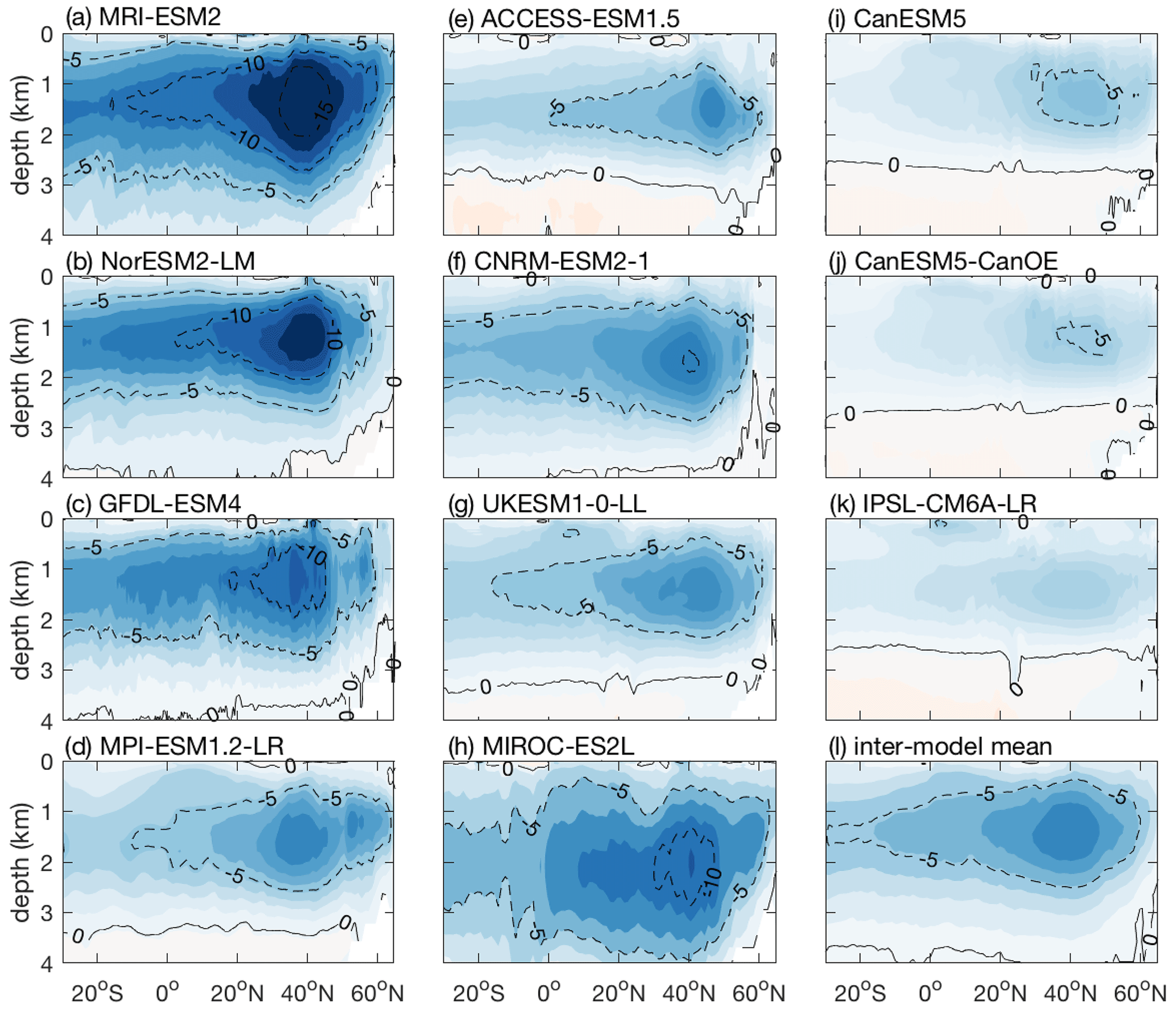
Figure 9Weakening of the Atlantic Meridional Overturning Circulation (AMOC; Sv), relative to the pre-industrial era: (a–k) 11 CMIP6 Earth system models and (l) their inter-model mean. The estimates are based on the fully coupled simulation (COU) under the 1 % yr−1 increasing CO2 experiment minus the pre-industrial control simulation (piControl). Diagnostics are from years 121 to 140 (the 20 years up to quadrupling of atmospheric CO2).
4.2 Results from CMIP6 Earth system models
The strength and weakening of the AMOC are diagnosed as the maximum pre-industrial AMOC between 30 and 50∘ N (Fig. 8) and the maximum AMOC change between 30 and 50∘ N (Fig. 9), respectively, in 11 CMIP6 Earth system models (Table 3). There is a large spread in the pre-industrial strength of the AMOC amongst the Earth system models (Fig. 8), with a range of 11.3 sverdrups (Sv) in IPSL-CM6A-LR to 23.2 Sv in NorESM2-LM (Table 3). There is also a large spread in the response of the AMOC to climate change amongst the models (Fig. 9), with the magnitude of the AMOC weakening ranging from −5.6 Sv in IPSL-CM6A-LR to −18.7 Sv in MRI-ESM2 (Table 3). Generally, the models with a stronger pre-industrial AMOC simulate a larger weakening in the AMOC with warming. Linear correlations are used to relate the AMOC variability amongst the models with the variability in the carbon cycle feedbacks for the global ocean and the different ocean basins (Table 4).
Table 3Carbon–concentration feedback parameter based on carbon storage, β* (PgC ppm−1), and carbon–climate feedback parameter based on carbon storage, γ* (PgC K−1), in the Atlantic Ocean, and the contribution from the saturated, disequilibrium and regenerated carbon pools, along with the strength of the Atlantic Meridional Overturning Circulation (AMOC) in sverdrups, in the pre-industrial era and its weakening relative to the pre-industrial era due to climate change. The strength and weakening of the AMOC are estimated as the maximum pre-industrial AMOC and maximum AMOC change between 30 and 50∘ N, respectively (Figs. 8 and 9). Results are shown for 11 CMIP6 Earth system models, along with the inter-model mean, standard deviation and coefficient of variation (CV), estimated as the standard deviation divided by the mean. The estimates are based on the fully coupled simulation (COU) and the biogeochemically coupled simulation (BGC) under the 1 % yr−1 increasing CO2 experiment. Diagnostics are from years 121 to 140 (the 20 years up to quadrupling of atmospheric CO2).
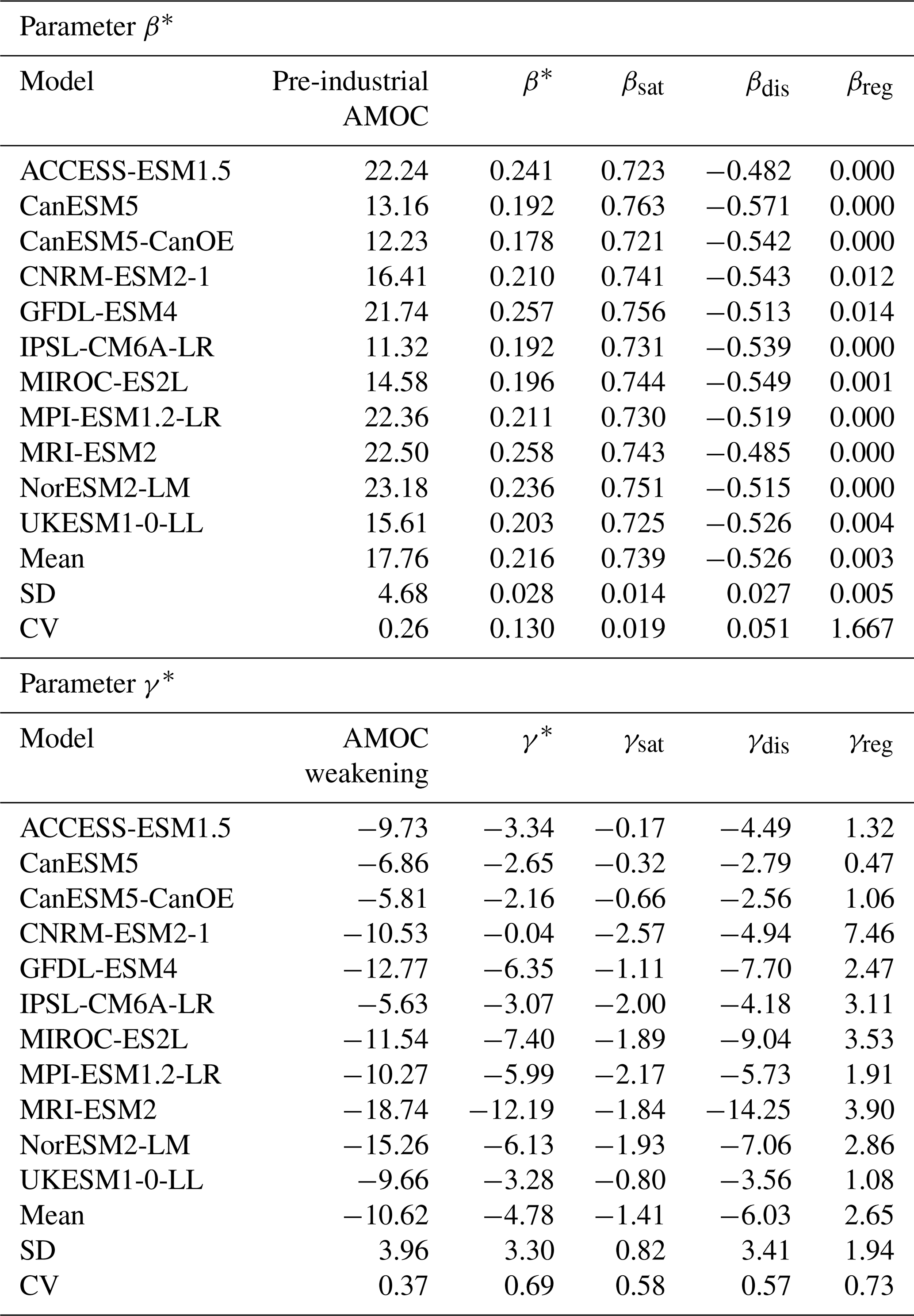
Table 4Correlation between the ocean carbon–concentration feedback parameter based on carbon storage, β*, and the pre-industrial strength of the Atlantic Meridional Overturning Circulation (AMOC) and correlation between the ocean carbon–climate feedback parameter based on carbon storage, γ*, and the AMOC weakening due to climate change, along with the contribution from the saturated, disequilibrium and regenerated carbon pools based on 11 CMIP6 models (Table 1). For the regenerated part of γ*, correlations estimated excluding the CNRM-ESM2-1 model, which has substantially larger changes in the regenerated carbon with warming than the rest of the Earth system models, are presented as . The correlation is expressed as a correlation coefficient, r, and a p value. The level of significance is assumed to be 0.05, and the statistically significant correlations with p<0.05 are highlighted by bold text. Diagnostics are from years 121 to 140 (the 20 years up to quadrupling of atmospheric CO2). Note that for the global ocean, β* and γ* are equivalent to β and γ.
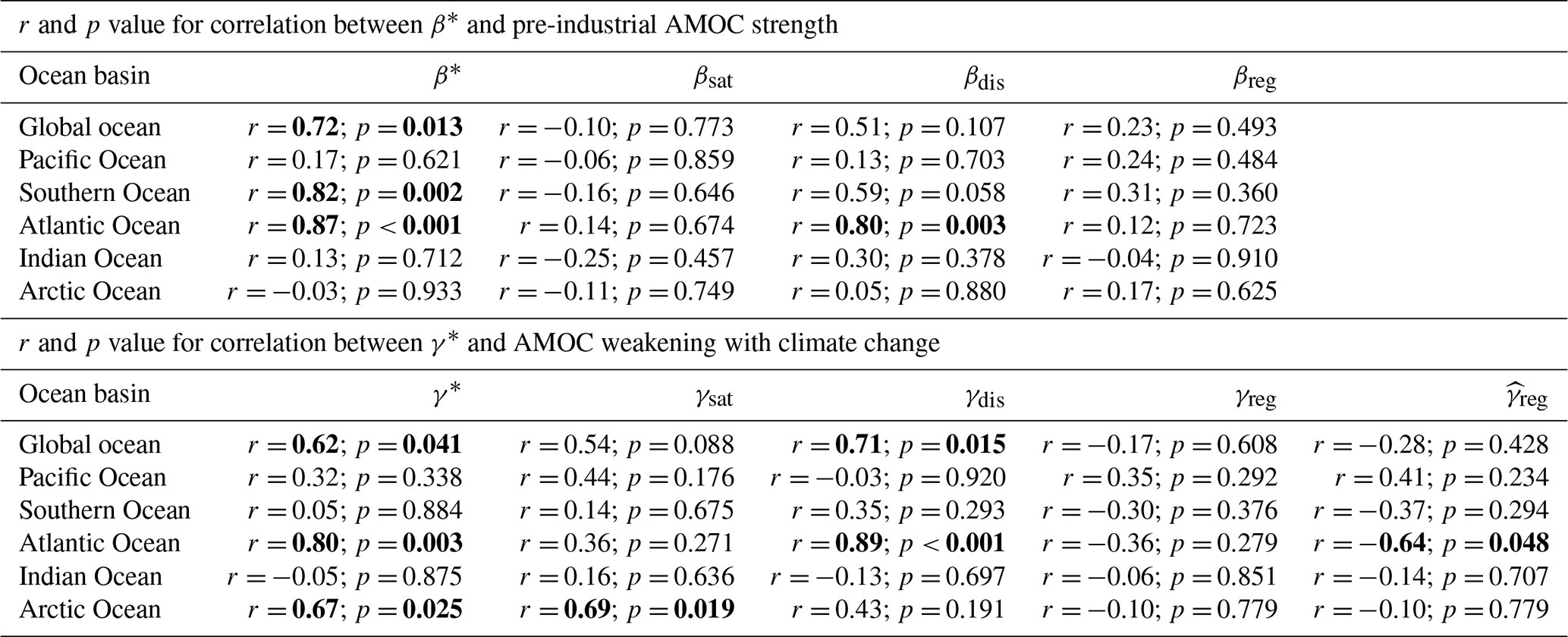
For the global ocean, there is a moderate positive correlation between the pre-industrial AMOC and the ocean carbon–concentration feedback parameter, β (r=0.72; Table 4), such that models with a stronger pre-industrial AMOC have a more positive β. However, there is no significant correlation between the pre-industrial AMOC and the saturated or disequilibrium part of β (Table 4) on the global scale. In the Atlantic Ocean, β* is strongly correlated with the pre-industrial AMOC in the Earth system models (r= 0.87), and this correlation is due to the contribution from βdis (Table 4 and Fig. 10a), which suggests that a stronger pre-industrial AMOC leads to a larger β* via a stronger physical transfer of anthropogenic carbon below the ocean surface there, which is similar to the behaviour of the idealised model (Fig. 7c).
In the Southern Ocean, there is a statistically significant correlation between the pre-industrial AMOC and β* (r=0.82) that is not associated with the saturated, the disequilibrium or the regenerated carbon pools (Table 4). A stronger pre-industrial AMOC is associated with a stronger return flow of interior water into the surface in the Southern Ocean upwelling branch of the overturning circulation (Marshall and Speer, 2012) and hence with stronger local anthropogenic carbon uptake from the atmosphere in the BGC run there. However, in the Southern Ocean both the anthropogenic carbon uptake from the atmosphere and its transport to the other basins are also controlled by subduction (Sabine et al., 2004; Sallée et al., 2012, 2013) and the residual circulation involving the wind-driven Ekman transport and eddy fluxes (Lauderdale et al., 2013). Hence, there is no significant correlation between the pre-industrial AMOC and βdis in the Southern Ocean as other processes involving subduction of mode and intermediate waters, as well as the residual circulation are important in setting the pre-industrial physical ventilation and transport of carbon to other basins. There is also no significant correlation between the pre-industrial AMOC and β* in the Pacific, Indian and Arctic oceans, which suggests that other processes dominate the ocean ventilation there.
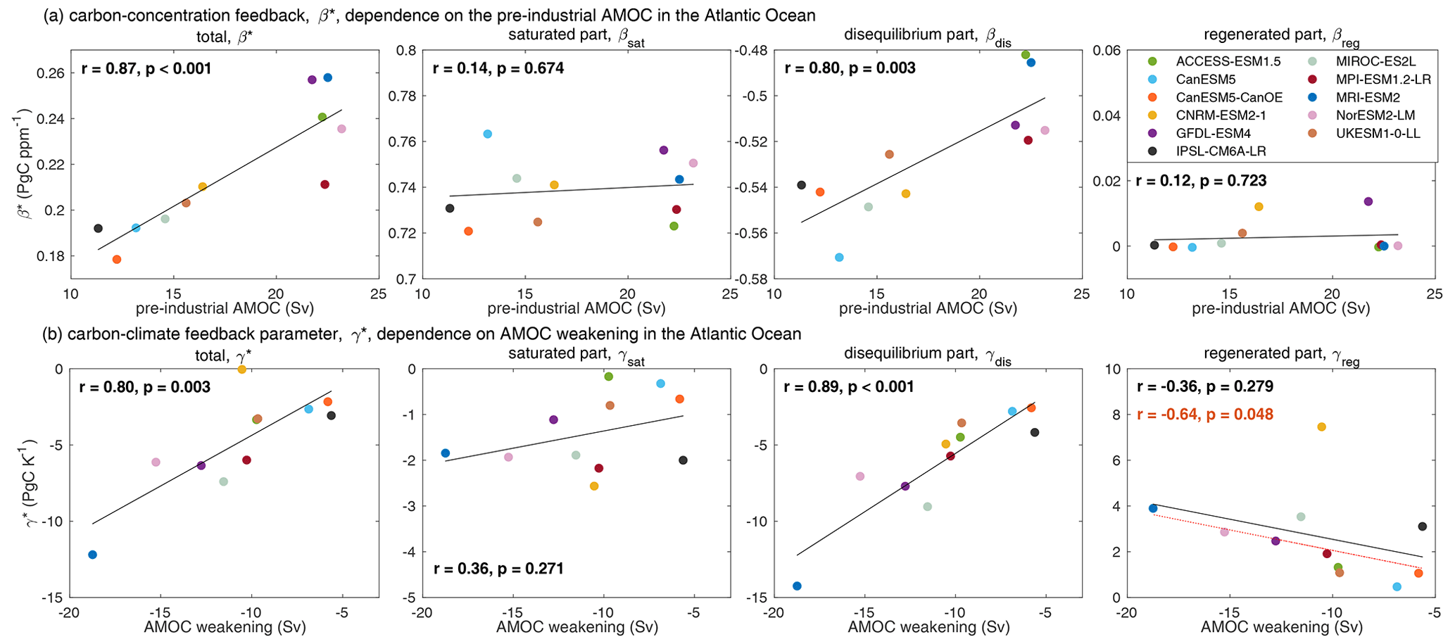
Figure 10(a) Dependence of the carbon–concentration feedback parameter based on carbon storage, β* (PgC ppm−1), on the pre-industrial strength of the Atlantic Meridional Overturning Circulation (AMOC; Sv), in the Atlantic Ocean, and (b) dependence of the carbon–climate feedback parameter based on carbon storage, γ* (PgC K−1), on the AMOC weakening with climate change in the Atlantic Ocean, in 11 CMIP6 models (Table 1), along with the contribution from the saturated, disequilibrium and regenerated carbon pools. The black lines correspond to the regression line based on an ordinary least-squares regression, with the corresponding correlation coefficient, r, and p value shown in each panel. The dashed red line and r and p value in red for γreg correspond to the regression line and the correlation coefficient estimated by excluding CNRM-ESM2-1, the model with the largest deviation from the rest of the Earth system models in terms of the regenerated carbon pool. The strength and weakening of the AMOC are estimated as the maximum pre-industrial AMOC and maximum AMOC change between 30 and 50∘ N, respectively (Table 3). Diagnostics are from years 121 to 140 (the 20 years up to quadrupling of atmospheric CO2).
For the global ocean, the carbon–climate feedback parameter, γ, and its disequilibrium part, γdis, are positively correlated with the AMOC weakening due to climate change in the Earth system models (r=0.62 and r=0.71, respectively, Table 4). This correlation for the global ocean is to first order driven by the Atlantic Ocean, as there is no significant correlation between AMOC weakening and γ* in the Pacific, Indian and Southern oceans or between AMOC weakening and γdis in the Arctic Ocean (Table 4). In the Atlantic Ocean, a more pronounced AMOC weakening due to climate change is associated with a larger reduction in the physical transfer of carbon below the ocean surface and so with a more negative γ* and γdis (Fig. 10b), consistent with the inferences for the idealised model (Fig. 7d). In the Arctic Ocean, there is a moderate correlation between γ* and AMOC weakening (r=0.67; Table 4). This correlation between γ* and AMOC weakening in the Arctic Ocean is associated with the carbonate chemistry and the saturated carbon pool, γsat (Table 4) and it appears to be related to changes in alkalinity (Supplement Fig. S3).
In the Atlantic Ocean, the correlation between γreg and AMOC weakening is negative (; Table 4), when excluding the CNRM-ESM2-1 model which has a much larger γreg than the rest of the Earth system models (Table 3). A more pronounced AMOC weakening leads to a longer residence time in the Atlantic Ocean interior and so to a larger accumulation of regenerated carbon there and a more positive γreg (Fig. 10b). The substantially larger change in the regenerated carbon pool with warming in CNRM-ESM2-1 compared to the rest of the models is probably due to a revised parameterisation for organic matter remineralisation (in PISCESv2-gas), its parameterisation of sedimentation and its interactive riverine input; see Séférian et al. (2020) for a discussion of differences in ocean biogeochemistry amongst the Earth system models.
Our study reveals the contribution of the Atlantic, Pacific, Southern, Indian and Arctic oceans to the ocean carbon cycle feedbacks in a set of CMIP6 Earth system models. This basin-scale contribution is explained in terms of the effect of the carbonate chemistry, physical ventilation and biological processes. Experiments using an idealised climate model and diagnostics of the CMIP6 models suggest a dependence of the ocean carbon cycle feedbacks on the strength of the pre-industrial Atlantic Meridional Overturning Circulation (AMOC) and on the magnitude of the AMOC weakening with warming.
The global ocean carbon–concentration feedback parameter, β, in CMIP6 models is controlled by competition between opposing contributions from the saturated and the disequilibrium carbon pools, such that (i) the carbonate chemistry drives a positive β that decreases with an increase in atmospheric CO2 as the ocean acidifies and its capacity to buffer atmospheric CO2 decreases and (ii) the physical ventilation drives a negative β that becomes less negative in time as the anthropogenic carbon is transferred from the ocean surface into the ocean interior. The global ocean carbon–climate feedback parameter, γ, in CMIP6 models is controlled by competition between the combined decrease in the saturated and disequilibrium carbon pools and the increase in the regenerated carbon pool, such that (i) the decrease in solubility and weakening in physical ventilation with warming drive a negative γ and (ii) the increase in the accumulation of regenerated carbon, associated with a longer residence time in the ocean interior with climate change, drives a positive γ.
5.1 Regional ocean carbon cycle feedbacks
The regional ocean carbon storage is controlled by the local air–sea carbon exchange and the transport of carbon by the ocean circulation. Here, the regional carbon cycle feedbacks are estimated from the regional ocean carbon storage so that the effect of the ocean transport of carbon is included in the feedbacks. This transport effect acts to decrease the carbon–concentration feedback parameter, β*, in the Southern Ocean and increase β* in the Southern Hemisphere subtropical gyres and the western boundary of the Atlantic Ocean in CMIP6 models. The transport effect on β* is consistent with the view that while almost half of the anthropogenic carbon enters through the Southern Ocean, much of this carbon is transferred and stored in the Atlantic, Pacific and Indian oceans (Sabine et al., 2004; Khatiwala et al., 2009; Frölicher et al., 2015). The transport effect also leads to a more spatially uniform and negative carbon–climate feedback parameter estimated in terms of carbon storage, γ*, compared with the carbon–climate feedback parameter estimated in terms of cumulative carbon uptake.
The Atlantic, Pacific and Southern oceans provide comparable contributions, of between 26 % and 30 %, to the global ocean carbon–concentration feedback, as estimated from the carbon storage, despite their different size. This large contribution from the Atlantic Ocean relative to its volume is associated with an enhanced physical transfer of anthropogenic carbon into the ocean interior due to strong local ventilation and transport of carbon from the Southern Ocean. The Arctic Ocean also provides a larger contribution to β* relative to its volume, consistent with observation-based estimates of anthropogenic carbon storage (Tanhua et al., 2009). The inter-model variability in the carbon–concentration feedback parameter, β*, as estimated by the coefficient of variation, is relatively small in all the ocean basins, reflecting the use of a similar carbonate chemistry scheme in these models (Séférian et al., 2020) and a similar general large-scale circulation.
The Atlantic Ocean has a large contribution to the ocean carbon–climate feedback relative to its size, as estimated from the carbon storage, in CMIP6 models, which is mainly due to the disequilibrium carbon pool. This result indicates that the Atlantic Ocean experiences a strong weakening in physical ventilation with climate change. Specifically, the negative γ* per unit area is largest in the high latitudes of the North Atlantic in CMIP6 models, consistent with γ diagnosed from the air–sea carbon fluxes in previous-generation Earth system models (Roy et al., 2011; Ciais et al., 2013). This response is in accord with previous studies suggesting the effect of climate-driven changes in the circulation on the carbon storage is significant in the North Atlantic (Sarmiento et al., 1998; Winton et al., 2013; Bernardello et al., 2014). The Arctic Ocean also has a large contribution to γ* relative to its size, primarily attributed to the saturated carbon pool and the large warming per unit volume in this basin.
The relative small contribution from the Southern Ocean to γ* in CMIP6 is due to partial compensation between the combined decrease in solubility and physical ventilation with warming, driving a negative γ*, and the large increase in accumulation of regenerated carbon in the ocean interior with climate change, driving a positive γ*. This compensation between the decrease in solubility and physical ventilation with warming and the increase in accumulation of regenerated carbon with climate change in the Southern Ocean is also supported by sensitivity model experiments (Sarmiento et al., 1998; Bernardello et al., 2014). A large increase in the regenerated carbon pool of the Southern Ocean with climate change was also found in CMIP5 models (Schwinger et al., 2014; Ito et al., 2015). In the Indo-Pacific Ocean, the carbon–climate feedback in CMIP6 is primarily attributed to the saturated carbon pool and the decrease in solubility with warming. This response in the Indo-Pacific Ocean is consistent with a feedback triggered by warming and the reduction in solubility dominating in low and middle latitudes, as revealed in a CMIP5 model (Rodgers et al., 2020) and diagnostics in previous-generation Earth system models (Roy et al., 2011; Ciais et al., 2013). The inter-model variability in γ* is mainly driven by the spread in the response of physical ventilation and circulation to climate change and in the parameterisation of ocean biogeochemical processes amongst the models.
5.2 Effect of the Atlantic Meridional Overturning Circulation
Our sensitivity experiments with an idealised climate model reveal that a weaker pre-industrial Atlantic Meridional Overturning Circulation (AMOC) leads to a smaller ocean carbon–concentration feedback parameter, β. This dependence of β on the pre-industrial AMOC is controlled by the disequilibrium carbon pool and the physical transfer of anthropogenic carbon from the surface to the ocean interior. The ocean carbon–climate feedback parameter, γ, is instead primarily controlled by the weakening in the AMOC with warming, which reduces the physical ventilation and leads to the disequilibrium part of γ becoming more negative in the idealised model.
Turning to the CMIP6 models, in the Atlantic Ocean, the carbon–concentration feedback parameter, β*, is strongly correlated to the strength of the pre-industrial AMOC. This correlation of β* to the AMOC is associated with the disequilibrium carbon pool and the effect of physical ventilation, such that Earth system models with a stronger AMOC provide more efficient transport of anthropogenic carbon into the ocean interior in the Atlantic Ocean, in accord with the behaviour in the idealised climate model. However, there is only a moderate correlation between AMOC strength and β on a global scale, which suggests that other processes related to ocean ventilation, involving the wind-driven gyre circulation, mode water formation and subduction, and the Southern Ocean residual circulation, are also important for controlling the ocean carbon–concentration feedback. In contrast with our results based on the idealised model and the CMIP6 models, Roy et al. (2011) found no direct dependence of β on the AMOC strength in older-generation Earth system models, which suggests that either (i) the sample of four models used in Roy et al. (2011) is too small to reveal the link between the AMOC and β or (ii) the dependence of β on AMOC strength is more pronounced when considering estimates at the quadrupling of atmospheric CO2 rather than estimates from years 2010 to 2100 in a high-emission scenario as in Roy et al. (2011).
In the Atlantic Ocean, the carbon–climate feedback parameter, γ*, is strongly correlated to the AMOC weakening with climate change in the CMIP6 models, similarly to the behaviour of the idealised climate model. This correlation of γ* to AMOC weakening is (i) primarily due to the disequilibrium carbon pool, with a more pronounced AMOC weakening driving a larger reduction in the physical transfer of carbon into the ocean interior and a more negative γ*, and (ii) to a lesser extent due to the regenerated carbon pool, with a more pronounced AMOC weakening driving a larger accumulation of regenerated carbon in the ocean interior and a more positive γ*. The dependence of the carbon–climate feedback on the AMOC weakening in the Atlantic Ocean is consistent with experiments using an older-generation Earth system model (Crueger et al., 2008; Yoshikawa et al., 2008). In the Arctic Ocean, there is moderate correlation between γ* and AMOC weakening in the CMIP6 models, with this correlation being associated with the saturated carbon pool and changes in carbonate chemistry. There is no significant correlation between γ* and AMOC weakening in the Pacific, Indian and Southern oceans. Hence, on a global and centennial scale, the weakening in the AMOC due to climate change has only a modest impact on ocean carbon uptake, consistent with previous studies (Sarmiento et al., 1998; Joos et al., 1999; Zickfeld et al., 2008).
A caveat in our analysis is that it does not reveal the control of the carbon cycle feedbacks by other ventilation processes beyond the AMOC, such as the formation and subduction of mode and intermediate waters involving the seasonal mixed-layer cycle, as well as the horizontal and vertical circulation. An analysis for the ocean carbon uptake and storage in dynamically based density space (Sallée et al., 2013; Meijers, 2014; Iudicone et al., 2016) is necessary to reveal the contribution of different water masses to β and γ (Tilla Roy, personal communication, 2020; Roy et al., 2021), and to better constrain the effect of local versus remote processes on the regional ocean carbon uptake and storage. Although our diagnostics reveal the relative contribution from the air–sea fluxes and the ocean transport of carbon to the regional carbon storage, further analysis is necessary to identify the effect of the ocean transport of carbon and other traces (e.g. temperature, salinity and nutrients) to the local air–sea fluxes.
In summary, in the 100-year time frame of our analysis, the Atlantic and Arctic oceans provide a large contribution to the carbon cycle feedbacks, as estimated in terms of carbon storage, relative to their size in CMIP6. This large contribution from the Atlantic Ocean is associated with the physical ventilation. The Southern Ocean has a relatively small contribution to the carbon–concentration feedback as estimated in terms of carbon storage, despite its large anthropogenic carbon uptake, due to large carbon transport to the other basins. The Southern Ocean also has a relatively small contribution to the carbon–climate feedback due to competing processes affecting the carbon storage in this basin. The more poorly ventilated Indo-Pacific Ocean has a small contribution to the carbon cycle feedbacks relative to its size. On a global and centennial scale, the carbon cycle feedbacks depend on the strength of the pre-industrial AMOC and its weakening with warming, such that (i) a stronger pre-industrial AMOC leads to a more positive carbon–concentration feedback and (ii) a more pronounced AMOC weakening due to climate change leads to a more negative carbon–climate feedback. Finally, for a quadrupling of atmospheric CO2 and on a centennial timescale, as considered in this study, the carbon–concentration feedback is substantially larger than the carbon–climate feedback; however, this will not necessarily be the case after the emissions cease and the system adjusts towards equilibrium.
The Southern Ocean accounts on average for about half of the ocean anthropogenic carbon uptake (Fig. A1a red line) in CMIP6 Earth system models despite covering only 27 % of the global ocean, which is consistent with results from CMIP5 model during the historical period (Frölicher et al., 2015), as well as with observation-based estimates (Mikaloff-Fletcher et al., 2006). However, a large portion of the anthropogenic carbon entering through the Southern Ocean is transported into the Atlantic, Indian and Pacific oceans, with the Atlantic Ocean receiving most of this carbon (Fig. A1a) in CMIP6 models, which is consistent with observation-based estimates (Sabine et al., 2004; Khatiwala et al., 2009). Consequently, the carbon–concentration feedback parameter estimated based on the regional cumulative carbon uptake, β (Fig. A1b, red lines) is substantially larger in the Southern Ocean but smaller in the Atlantic, Pacific and Indian oceans than when estimated based on the regional carbon storage, β* (Fig. A1b, black lines). The feedback parameter β is also smaller than β* in the Arctic Ocean indicating that ocean transport supplies anthropogenic carbon to the Arctic in CMIP6 models.
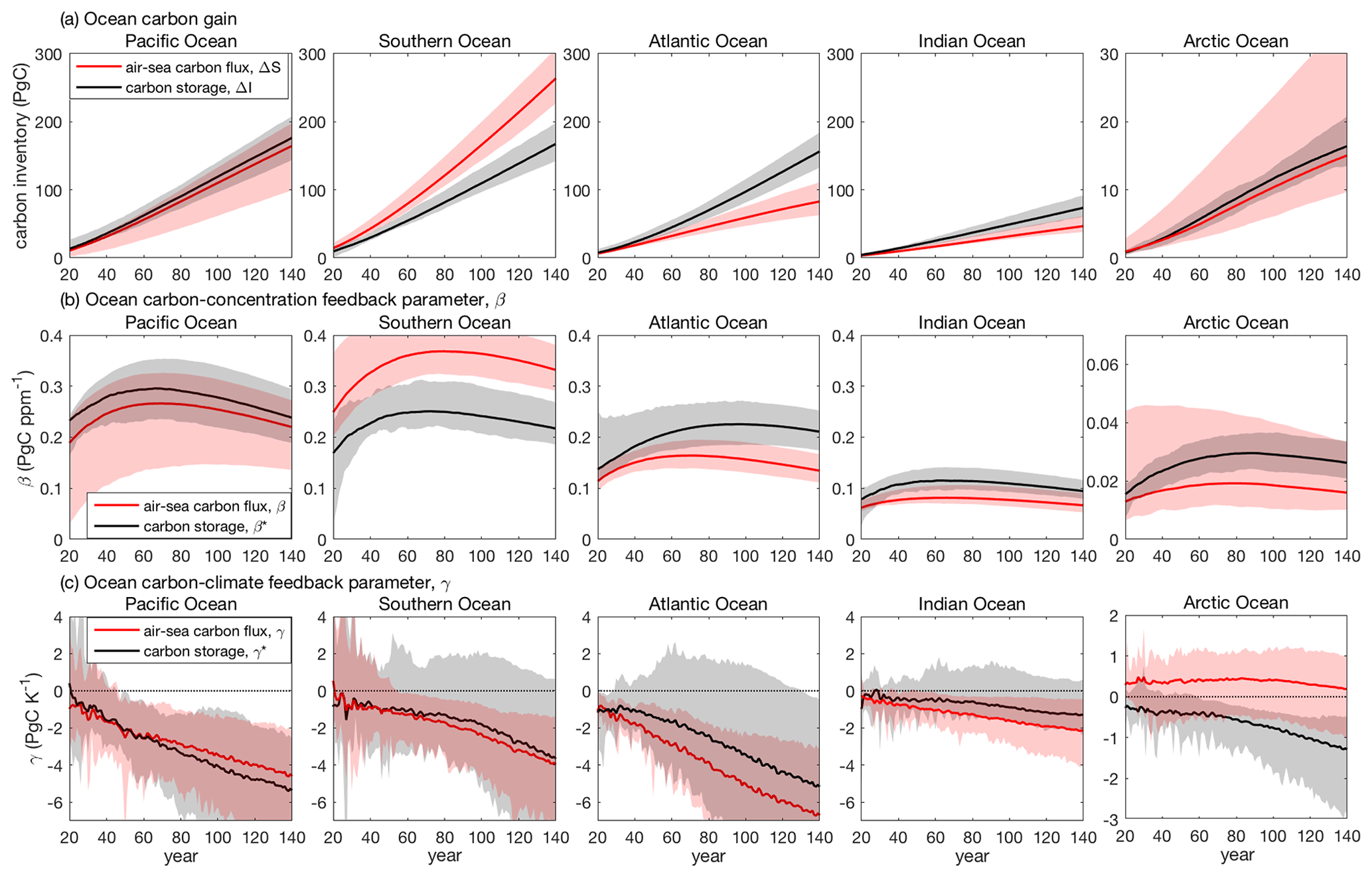
Figure A1Ocean carbon storage and cumulative air–sea carbon flux in the Pacific, Southern, Atlantic, Indian and Arctic oceans in CMIP6 Earth system models, along with the ocean carbon cycle feedback parameters: (a) changes in the ocean carbon storage, ΔI, and cumulative ocean carbon uptake, Δ𝒮, in petagrams of carbon, in the fully coupled simulations (COU) relative to the pre-industrial era; (b) carbon–concentration feedback parameter based on carbon storage, β* (PgC ppm−1), and based on the cumulative carbon uptake, β (PgC ppm−1); and (c) carbon–climate feedback parameter based on carbon storage, γ* (PgC K−1), and based on the cumulative carbon uptake, γ (PgC K−1). The solid lines and the shading show the model mean and the model range, respectively, based on the 1 % yr−1 increasing CO2 experiment over 140 years in 11 CMIP6 models (Table 1). The estimates for the feedback parameters are based on the fully coupled simulation (COU) and the biogeochemically coupled simulation (BGC).
The net effect of climate change is a carbon loss from the ocean to the atmosphere and a negative γ in the Atlantic, Indian, Pacific and Southern oceans (Fig. A1c, red lines). The ocean transport acts to reduce the negative γ in the Atlantic, Indian and Southern oceans but to increase the negative γ in the Pacific Ocean (Fig. A1c, compare the red with the black lines). In contrast, in the Arctic Ocean, the decrease in sea-ice coverage due to climate change leads to an increase in the ocean carbon uptake from the atmosphere and a positive γ. The ocean transport opposes this ocean gain in carbon from the atmosphere in the Arctic and leads to a reduction in the ocean carbon inventory and a negative γ* (Fig. A1c, black lines).
The saturated part of β* is positive everywhere in the ocean (Fig. B1a). By definition, βsat depends on the ocean volume, so it is larger in deeper regions. The disequilibrium part of β* is small on the shelves and in the well-ventilated North Atlantic and large in the more poorly ventilated Pacific Ocean and in deep-ocean regions (Fig. B1a). This vertically integrated regional view for the carbon storage reflects that in the BGC simulation, ΔDICdis is small in the upper ocean but large and negative in deeper water outside the North Atlantic (see Figs. 10 and 11 in Arora et al., 2020). The regenerated part of β* is negligible in the CMIP6 models.
The saturated part of γ* is negative and large in the Arctic Ocean (Fig. B1b), reflecting a large decrease in solubility due to large warming per unit volume (Fig. 1d). Along the western boundary of the North Atlantic Ocean, γsat is slightly positive (Fig. B1b), which is related to a large regional gain in carbon (Fig. 2a), acting to reduce the carbonate system sensitivity to changes in temperature (see Eq. 20), combined with a regional increase in alkalinity due to climate change. The disequilibrium part of γ* is negative and large in the North Atlantic, along the western boundary of the Atlantic Ocean and in the Southern Ocean, indicating that the effect of weakening in the ventilation is significant in these regions. In the Arctic Ocean, the decrease in sea-ice coverage drives an increase in the ocean carbon uptake and leads to areas with a large positive γdis. The regenerated part of γ* has a similar spatial pattern but is of opposite sign to γdis (Fig. B1b), which suggests that γreg is dominated by changes in the ocean ventilation. Along the Equator and in the eastern boundary upwelling regions, γdis and γreg are slightly positive and negative, respectively. This negative γreg and positive γdis in regions of upwelling is consistent with a coupling between the regenerated and the disequilibrium carbon pools, such that a positive ΔDICreg brought into the surface waters from depth leads to an excess of carbon at the surface that is converted into a positive ΔDICdis (i.e. oversaturation) (Ito and Follows, 2013).

Figure B1Geographical distribution of the CMIP6 inter-model mean contribution from the saturated, disequilibrium and regenerated carbon pools to the carbon cycle feedback parameters estimated based on carbon storage, β* and γ*, normalised by area: (a) βsat, βdis and βreg (gC ppm−1 m−2) and (b) γsat, γdis and γreg (gC K−1 m−2). The estimates are based on the fully coupled simulation (COU) and the biogeochemically coupled simulation (BGC) under the 1 % yr−1 increasing CO2 experiment. Diagnostics are from years 121 to 140 (the 20 years up to quadrupling of atmospheric CO2). The inter-model mean is based on the models in Table 1.
The data used here are from the CMIP6 simulations performed by the various modelling groups and available from the CMIP6 archive (https://esgf-node.llnl.gov/search/cmip6, World Climate Research Programme, 2021). The specific datasets used for each of the models are (i) ACCESS-ESM1.5 (Ziehn et al., 2019a, b, c), (ii) CanESM5 (Swart et al., 2019a, b, c), (iii) CanESM5-CanOE (Swart et al., 2019d, e, f), (iv) CNRM-ESM2-1 (Seferian, 2018a, b, c), (v) GFDL-ESM4 (Krasting et al., 2018a, b, c), (vi) IPSL-CM6A-LR (Boucher et al., 2018a, b, c), (vii) MIROC-ES2L (Hajima et al., 2019a, b, c), (viii) MPI-ESM1.2-LR (Brovkin et al., 2019; Wieners et al., 2019a, b), (ix) MRI-ESM2 (Yukimoto et al., 2019a, b, c), (x) NorESM2-LM (Schwinger et al., 2020; Seland et al., 2019a, b), and (xi) UKESM1.0-LL (Jones, 2019; Tang et al., 2019a, b).
The supplement related to this article is available online at: https://doi.org/10.5194/bg-18-3189-2021-supplement.
AK conducted the analysis and led the interpretation of the results and writing of the manuscript. RGW contributed to the design of the analysis, the interpretation of the results and the writing of the manuscript.
The authors declare that they have no conflict of interest.
The authors acknowledge the World Climate Research Programme, which, through its Working Group on Coupled Modelling, coordinated and promoted CMIP6; the climate modelling groups for producing and making available their model output; and the Earth System Grid Federation for archiving the data and providing access. We thank Jörg Schwinger and the anonymous reviewer for their constructive comments.
This research has been supported by the Natural Environment Research Council (grant nos. NE/T007788/1 and NE/T010657/1).
This paper was edited by Fortunat Joos and reviewed by Jörg Schwinger and one anonymous referee.
Arora, V. K., Boer, G. J., Friedlingstein, P., Eby, M., Jones, C. D., Christian, J. R., Bonan, G., Bopp, L., Brovkin, V., Cadule, P., Hajima, T., Ilyina, T., Lindsay, K., Tjiputra, J. F., and Wu, T.: Carbon-Concentration and Carbon-Climate Feedbacks in CMIP5 Earth System Models, J. Climate, 26, 5289–5314, https://doi.org/10.1175/JCLI-D-12-00494.1, 2013. a, b
Arora, V. K., Katavouta, A., Williams, R. G., Jones, C. D., Brovkin, V., Friedlingstein, P., Schwinger, J., Bopp, L., Boucher, O., Cadule, P., Chamberlain, M. A., Christian, J. R., Delire, C., Fisher, R. A., Hajima, T., Ilyina, T., Joetzjer, E., Kawamiya, M., Koven, C. D., Krasting, J. P., Law, R. M., Lawrence, D. M., Lenton, A., Lindsay, K., Pongratz, J., Raddatz, T., Séférian, R., Tachiiri, K., Tjiputra, J. F., Wiltshire, A., Wu, T., and Ziehn, T.: Carbon–concentration and carbon–climate feedbacks in CMIP6 models and their comparison to CMIP5 models, Biogeosciences, 17, 4173–4222, https://doi.org/10.5194/bg-17-4173-2020, 2020. a, b, c, d, e, f, g, h, i, j, k
Bernardello, R., Marinov, I., Palter, J. B., Sarmiento, J. L., Galbraith, E. D., and Slater, R. D.: Response of the Ocean Natural Carbon Storage to Projected Twenty-First-Century Climate Change, J. Climate, 27, 2033–2053, https://doi.org/10.1175/JCLI-D-13-00343.1, 2014. a, b, c, d, e, f
Boer, G. J. and Arora, V.: Temperature and concentration feedbacks in the carbon cycle, Geophys. Res. Lett., 36, L02704, https://doi.org/10.1029/2008GL036220, 2009. a
Boer, G. J. and Arora, V.: Geographic Aspects of Temperature and Concentration Feedbacks in the Carbon Budget, J. Climate, 23, 775–784, https://doi.org/10.1175/2009JCLI3161.1, 2010. a
Boucher, O., Denvil, S., Levavasseur, G., Cozic, A., Caubel, A., Foujols, M.-A., Meurdesoif, Y., Cadule, P., Devilliers, M., Ghattas, J., Lebas, N., Lurton, T., Mellul, L., Musat, I., Mignot, J., and Cheruy, F.: IPSL IPSL-CM6A-LR model output prepared for CMIP6 CMIP 1pctCO2, Version: 20190305, Earth System Grid Federation, https://doi.org/10.22033/ESGF/CMIP6.5049, 2018a. a
Boucher, O., Denvil, S., Levavasseur, G., Cozic, A., Caubel, A., Foujols, M.-A., Meurdesoif, Y., Cadule, P., Devilliers, M., Ghattas, J., Lebas, N., Lurton, T., Mellul, L., Musat, I., Mignot, J., and Cheruy, F.: IPSL IPSL-CM6A-LR model output prepared for CMIP6 CMIP piControl, Version: 20200326, Earth System Grid Federation, https://doi.org/10.22033/ESGF/CMIP6.5251, 2018b. a
Boucher, O., Denvil, S., Levavasseur, G., Cozic, A., Caubel, A., Foujols, M.-A., Meurdesoif, Y., Cadule, P., and Ghattas, J.: IPSL IPSL-CM6A-LR model output prepared for CMIP6 C4MIP 1pctCO2-bgc, Version: 20180914, Earth System Grid Federation, https://doi.org/10.22033/ESGF/CMIP6.5050, 2018c. a
Boucher, O., Servonnat, J., Albright, A. L., Aumont, O., Balkanski, Y., Bastrikov, V., Bekki, S., Bonnet, R., Bony, S., Bopp, L., Braconnot, P., Brockmann, P., Cadule, P., Caubel, A., Cheruy, F., Codron, F., Cozic, A., Cugnet, D., D'Andrea, F., Davini, P., de Lavergne, C., Denvil, S., Deshayes, J., Devilliers, M., Ducharne, A., Dufresne, J.-L., Dupont, E., Éthé, C., Fairhead, L., Falletti, L., Flavoni, S., Foujols, M.-A., Gardoll, S., Gastineau, G., Ghattas, J., Grandpeix, J.-Y., Guenet, B., Guez, Lionel, E., Guilyardi, E., Guimberteau, M., Hauglustaine, D., Hourdin, F., Idelkadi, A., Joussaume, S., Kageyama, M., Khodri, M., Krinner, G., Lebas, N., Levavasseur, G., Lévy, C., Li, L., Lott, F., Lurton, T., Luyssaert, S., Madec, G., Madeleine, J.-B., Maignan, F., Marchand, M., Marti, O., Mellul, L., Meurdesoif, Y., Mignot, J., Musat, I., Ottlé, C., Peylin, P., Planton, Y., Polcher, J., Rio, C., Rochetin, N., Rousset, C., Sepulchre, P., Sima, A., Swingedouw, D., Thiéblemont, R., Traore, A. K., Vancoppenolle, M., Vial, J., Vialard, J., Viovy, N., and Vuichard, N.: Presentation and Evaluation of the IPSL-CM6A-LR Climate Model, J. Adv. Model. Earth Sy., 12, e2019MS002010, https://doi.org/10.1029/2019MS002010, 2020. a
Bronselaer, B. and Zanna, L.: Heat and carbon coupling reveals ocean warming due to circulation changes, Nature, 584, 227–233, https://doi.org/10.1038/s41586-020-2573-5, 2020. a
Brovkin, V., Wieners, K.-H., Giorgetta, M., Jungclaus, J., Reick, C., Esch, M., Bittner, M., Legutke, S., Schupfner, M., Wachsmann, F., Gayler, V., Haak, H., de Vrese, P., Raddatz, T., Mauritsen, T., von Storch, J.-S., Behrens, J., Claussen, M., Crueger, T., Fast, I., Fiedler, S., Hagemann, S., Hohenegger, C., Jahns, T., Kloster, S., Kinne, S., Lasslop, G., Kornblueh, L., Marotzke, J., Matei, D., Meraner, K., Mikolajewicz, U., Modali, K., Müller, W., Nabel, J., Notz, D., Peters, K., Pincus, R., Pohlmann, H., Pongratz, J., Rast, S., Schmidt, H., Schnur, R., Schulzweida, U., Six, K., Stevens, B., Voigt, A., and Roeckner, E.: MPI-M MPI-ESM1.2-LR model output prepared for CMIP6 C4MIP 1pctCO2-bgc, Version: 20190710, Earth System Grid Federation, https://doi.org/10.22033/ESGF/CMIP6.6437, 2019. a
Ceppi, P. and Gregory, J. M.: Relationship of tropospheric stability to climate sensitivity and Earth's observed radiation budget, P. Natl. Acad. Sci. USA, 114, 13126–13131, https://doi.org/10.1073/pnas.1714308114, 2017. a
Cheng, W., Chiang, J. C. H., and Zhang, D.: Atlantic Meridional Overturning Circulation (AMOC) in CMIP5 Models: RCP and Historical Simulations, J. Climate, 26, 7187–7197, https://doi.org/10.1175/JCLI-D-12-00496.1, 2013. a
Ciais, P., Sabine, C., Bala, G., Bopp, L., Brovkin, V., Canadell, J., Chhabra, A., DeFries, R., Galloway, J., Heimann, M., Jones, C., Quéré, C. L., Myneni, R., Piao, S., and Thornton, P.: Carbon and Other Biogeochemical Cycles, in: Climate Change 2013: The Physical Science Basis, Contribution of Working Group I to the Fifth Assessment Report of the Intergovernmental Panel on Climate Change, Cambridge University Press, Cambridge, UK, 2013. a, b
Crueger, T., Roeckner, E., Raddatz, T., Schnur, R., and Wetzel, P.: Ocean dynamics determine the response of oceanic CO2 uptake to climate change, Clim. Dynam., 31, 151–168, https://doi.org/10.1007/s00382-007-0342-x, 2008. a, b, c
Dunne, J. P., Horowitz, L. W., Adcroft, A. J., Ginoux, P., Held, I. M., John, J. G., Krasting, J. P., Malyshev, S., Naik, V., Paulot, F., Shevliakova, E., Stock, C. A., Zadeh, N., Balaji, V., Blanton, C., Dunne, K. A., Dupuis, C., Durachta, J., Dussin, R., Gauthier, P. P. G., Griffies, S. M., Guo, H., Hallberg, R. W., Harrison, M., He, J., Hurlin, W., McHugh, C., Menzel, R., Milly, P. C. D., Nikonov, S., Paynter, D. J., Ploshay, J., Radhakrishnan, A., Rand, K., Reichl, B. G., Robinson, T., Schwarzkopf, D. M., Sentman, L. T., Underwood, S., Vahlenkamp, H., Winton, M., Wittenberg, A. T., Wyman, B., Zeng, Y., and Zhao, M.: The GFDL Earth System Model Version 4.1 (GFDL-ESM 4.1): Overall Coupled Model Description and Simulation Characteristics, J. Adv. Model. Earth Sy., 12, e2019MS002015, https://doi.org/10.1029/2019MS002015, 2020. a
Follows, M. J., Ito, T., and Dutkiewicz, S.: On the solution of the carbonate chemistry system in ocean biogeochemistry models, Ocean Model., 12, 290–301, https://doi.org/10.1016/j.ocemod.2005.05.004, 2006. a, b
Friedlingstein, P., Dufrense, J.-L., Cox, P. M., and Rayner, P.: How positive is the feedback between climate change and the carbon cycle?, Tellus B, 55, 692–700, https://doi.org/10.1034/j.1600-0889.2003.01461.x, 2003. a, b
Friedlingstein, P., Cox, P., Betts, R., Bopp, L., von Bloh, W., Brovkin, V., Cadule, P., Doney, S., Eby, M., Fung, I., Bala, G., John, J., Jones, C., Joos, F., Kato, T., Kawamiya, M., Knorr, W., Lindsay, K., Matthews, H. D., Raddatz, T., Rayner, P., Reick, C., Roeckner, E., Schnitzler, K.-G., Schnur, R., Strassmann, K., Weaver, A. J., Yoshikawa, C., and Zeng, N.: Climate-Carbon Cycle Feedback Analysis: Results from the C4MIP Model Intercomparison, J. Climate, 19, 3337–3353, https://doi.org/10.1175/JCLI3800.1, 2006. a, b, c
Frölicher, T. L., Sarmiento, J. L., Paynter, D. J., Dunne, J. P., Krasting, J. P., and Winton, M.: Dominance of the Southern Ocean in Anthropogenic Carbon and Heat Uptake in CMIP5 Models, J. Climate, 28, 862–886, https://doi.org/10.1175/JCLI-D-14-00117.1, 2015. a, b, c
Gnanadesikan, A.: A simple predictive model of the structure of the oceanic pycnocline, Science, 283, 2077–2081, https://doi.org/10.1126/science.283.5410.2077, 1999. a
Gregory, J. M., Ingram, W. J., Palmer, M. A., Jones, G. S., Stott, P. A., Thorpe, R. B., Lowe, J. A., Johns, T. C., and Williams, K. D.: A new method for diagnosing radiative forcing and climate sensitivity, Geophys. Res. Lett., 31, L03205, https://doi.org/10.1029/2003GL018747, 2004. a
Gregory, J. M., Jones, C. D., Cadule, P., and Friedlingstein, P.: Quantifying Carbon Cycle Feedbacks, J. Climate, 22, 5232–5250, https://doi.org/10.1175/2009JCLI2949.1, 2009. a, b
Gruber, N., Sarmiento, J., and Stocker, T.: An improved method for detecting anthropogenic CO2 in the oceans, Global Biogeochem. Cy., 10, 809–837, https://doi.org/10.1029/96GB01608, 1996. a
Hajima, T., Abe, M., Arakawa, O., Suzuki, T., Komuro, Y., Ogura, T., Ogochi, K.,Watanabe, M., Yamamoto, A., Tatebe, H., Noguchi, M. A., Ohgaito, R., Ito, A., Yamazaki, D., Ito, A., Takata, K.,Watanabe, S., Kawamiya, M., and Tachiiri, K.: MIROC MIROC-ES2L model output prepared for CMIP6 CMIP 1pctCO2, Version: 20200731, Earth System Grid Federation, https://doi.org/10.22033/ESGF/CMIP6.5370, 2019a. a
Hajima, T., Abe, M., Arakawa, O., Suzuki, T., Komuro, Y., Ogura, T., Ogochi, K.,Watanabe, M., Yamamoto, A., Tatebe, H., Noguchi, M. A., Ohgaito, R., Ito, A., Yamazaki, D., Ito, A., Takata, K.,Watanabe, S., Kawamiya, M., and Tachiiri, K.: MIROC MIROC-ES2L model output prepared for CMIP6 CMIP piControl, Version: 20200731, Earth System Grid Federation, https://doi.org/10.22033/ESGF/CMIP6.5710, 2019b. a
Hajima, T., Kawamiya, M., Tachiiri, K., Abe, M., Arakawa, O., Suzuki, T., Komuro, Y., Ogochi, K.,Watanabe, M., Yamamoto, A., Tatebe, H., Noguchi, M. A., Ohgaito, R., Ito, A., Yamazaki, D., Ito, A., Takata, K., and Watanabe, S.: MIROC MIROC-ES2L model output prepared for CMIP6 C4MIP 1pctCO2-bgc, Version: 20200731, Earth System Grid Federation, https://doi.org/10.22033/ESGF/CMIP6.5376, 2019c. a
Hajima, T., Watanabe, M., Yamamoto, A., Tatebe, H., Noguchi, M. A., Abe, M., Ohgaito, R., Ito, A., Yamazaki, D., Okajima, H., Ito, A., Takata, K., Ogochi, K., Watanabe, S., and Kawamiya, M.: Development of the MIROC-ES2L Earth system model and the evaluation of biogeochemical processes and feedbacks, Geosci. Model Dev., 13, 2197–2244, https://doi.org/10.5194/gmd-13-2197-2020, 2020. a
Ito, T. and Follows, M. J.: Preformed phosphate, soft tissue pump and atmospheric CO2, J. Mar. Res., 63, 813–839, https://doi.org/10.1357/0022240054663231, 2005. a, b
Ito, T. and Follows, M. J.: Air-sea disequilibrium of carbon dioxide enhances the biological carbon sequestration in the Southern Ocean, Global Biogeochem. Cy., 27, 1129–1138, https://doi.org/10.1002/2013GB004682, 2013. a
Ito, T., Bracco, A., Deutsch, C., Frenzel, H., Long, M., and Takano, Y.: Sustained growth of the Southern Ocean carbon storage in a warming climate, Geophys. Res. Lett., 42, 4516–4522, https://doi.org/10.1002/2015GL064320, 2015. a
Iudicone, D., Rodgers, K. B., Plancherel, Y., Aumont, O., Ito, T., Key, R. M., Madec, G., and Ishii, M.: The formation of the ocean's anthropogenic carbon reservoir, Sci. Rep.-UK, 6, 35473, https://doi.org/10.1038/srep35473, 2016. a
Johnson, H. L., Marshall, D. P., and Sproson, D. A. J.: Reconciling theories of a mechanically driven meridional overturning circulation with thermohaline forcing and multiple equilibria, Clim. Dynam., 29, 821–836, https://doi.org/10.1007/s00382-007-0262-9, 2007. a
Jones, C.: MOHC UKESM1.0-LL model output prepared for CMIP6 C4MIP 1pctCO2-bgc, Earth System Grid Federation, https://doi.org/10.22033/ESGF/CMIP6.5796, 2019. a
Jones, C. D., Arora, V., Friedlingstein, P., Bopp, L., Brovkin, V., Dunne, J., Graven, H., Hoffman, F., Ilyina, T., John, J. G., Jung, M., Kawamiya, M., Koven, C., Pongratz, J., Raddatz, T., Randerson, J. T., and Zaehle, S.: C4MIP – The Coupled Climate–Carbon Cycle Model Intercomparison Project: experimental protocol for CMIP6, Geosci. Model Dev., 9, 2853–2880, https://doi.org/10.5194/gmd-9-2853-2016, 2016. a, b
Joos, F., Plattner, G.-K., Stocker, T. F., Marchal, O., and Schmittner, A.: Global Warming and Marine Carbon Cycle Feedbacks on Future Atmospheric CO2, Science, 284, 464–467, https://doi.org/10.1126/science.284.5413.464, 1999. a, b, c
Katavouta, A., Williams, R. G., Goodwin, P., and Roussenov, V.: Reconciling Atmospheric and Oceanic Views of the Transient Climate Response to Emissions, Geophys. Res. Lett., 45, 6205–6214, https://doi.org/10.1029/2018GL077849, 2018. a
Katavouta, A., Williams, R. G., and Goodwin, P.: The Effect of Ocean Ventilation on the Transient Climate Response to Emissions, J. Climate, 32, 5085–5105, https://doi.org/10.1175/JCLI-D-18-0829.1, 2019. a, b
Krasting, J. P., Blanton, C., McHugh, C., Radhakrishnan, A., John, J. G., Rand, K., Nikonov, S., Vahlenkamp, H., Zadeh, N. T., Dunne, J. P., Shevliakova, E., Horowitz, L. W., Stock, C., Malyshev, S., Ploshay, J., Gauthier, P. P., Naik, V., Winton, M., and Zeng, Y.: NOAA-GFDL GFDL-ESM4 model output prepared for CMIP6 C4MIP 1pctCO2-bgc, Version: 20180701, Earth System Grid Federation, https://doi.org/10.22033/ESGF/CMIP6.8475, 2018a. a
Krasting, J. P., John, J. G., Blanton, C., McHugh, C., Nikonov, S., Radhakrishnan, A., Rand, K., Zadeh, N. T., Balaji, V., Durachta, J., Dupuis, C., Menzel, R., Robinson, T., Underwood, S., Vahlenkamp, H., Dunne, K. A., Gauthier, P. P., Ginoux, P., Griffies, S. M., Hallberg, R., Harrison, M., Hurlin, W., Malyshev, S., Naik, V., Paulot, F., Paynter, D. J., Ploshay, J., Reichl, B. G., Schwarzkopf, D. M., Seman, C. J., Silvers, L., Wyman, B., Zeng, Y., Adcroft, A., Dunne, J. P., Dussin, R., Guo, H., He, J., Held, I. M., Horowitz, L. W., Lin, P., Milly, P., Shevliakova, E., Stock, C., Winton, M., Wittenberg, A. T., Xie, Y., and Zhao, M.: NOAA-GFDL GFDL-ESM4 model output prepared for CMIP6 CMIP 1pctCO2, Version: 20180701, Earth System Grid Federation, https://doi.org/10.22033/ESGF/CMIP6.8473, 2018b. a
Krasting, J. P., John, J. G., Blanton, C., McHugh, C., Nikonov, S., Radhakrishnan, A., Rand, K., Zadeh, N. T., Balaji, V., Durachta, J., Dupuis, C., Menzel, R., Robinson, T., Underwood, S., Vahlenkamp, H., Dunne, K. A., Gauthier, P. P., Ginoux, P., Griffies, S. M., Hallberg, R., Harrison, M., Hurlin, W., Malyshev, S., Naik, V., Paulot, F., Paynter, D. J., Ploshay, J., Reichl, B. G., Schwarzkopf, D. M., Seman, C. J., Silvers, L., Wyman, B., Zeng, Y., Adcroft, A., Dunne, J. P., Dussin, R., Guo, H., He, J., Held, I. M., Horowitz, L. W., Lin, P., Milly, P., Shevliakova, E., Stock, C., Winton, M., Wittenberg, A. T., Xie, Y., and Zhao, M.: NOAA-GFDL GFDL-ESM4 model output prepared for CMIP6 CMIP piControl, Version: 20180701, Earth System Grid Federation, https://doi.org/10.22033/ESGF/CMIP6.8669, 2018c. a
Khatiwala, S., Primeau, F., and Hall, T.: Reconstruction of the history of anthropogenic CO2 concentrations in the ocean, Nature, 462, 346–349, https://doi.org/10.1038/nature08526, 2009. a, b
Lauderdale, J. M., Naveira-Garabato, A. C., Oliver, K. I. C., Follows, M. J., and Williams, R. G.: Wind-driven changes in Southern Ocean residual circulation, ocean carbon reservoirs and atmospheric CO2, Clim. Dynam., 41, 2145–2164, https://doi.org/10.1007/s00382-012-1650-3, 2013. a, b, c
Marshall, D. P. and Zanna, L.: A Conceptual Model of Ocean Heat Uptake under Climate Change, J. Climate, 27, 8444–8465, https://doi.org/10.1175/JCLI-D-13-00344.1, 2014. a
Marshall, J. and Speer, K.: Closure of the meridional overturning circulation through Southern Ocean upwelling, Nat. Geosci., 5, 171–180, https://doi.org/10.1038/ngeo1391, 2012. a
Mauritsen, T., Bader, J., Becker, T., Behrens, J., Bittner, M., Brokopf, R., Brovkin, V., Claussen, M., Crueger, T., Esch, M., Fast, I., Fiedler, S., Fläschner, D., Gayler, V., Giorgetta, M., Goll, D. S., Haak, H., Hagemann, S., Hedemann, C., Hohenegger, C., Ilyina, T., Jahns, T., Jimenéz-de-la Cuesta, D., Jungclaus, J., Kleinen, T., Kloster, S., Kracher, D., Kinne, S., Kleberg, D., Lasslop, G., Kornblueh, L., Marotzke, J., Matei, D., Meraner, K., Mikolajewicz, U., Modali, K., Möbis, B., Müller, W. A., Nabel, J. E. M. S., Nam, C. C. W., Notz, D., Nyawira, S.-S., Paulsen, H., Peters, K., Pincus, R., Pohlmann, H., Pongratz, J., Popp, M., Raddatz, T. J., Rast, S., Redler, R., Reick, C. H., Rohrschneider, T., Schemann, V., Schmidt, H., Schnur, R., Schulzweida, U., Six, K. D., Stein, L., Stemmler, I., Stevens, B., von Storch, J.-S., Tian, F., Voigt, A., Vrese, P., Wieners, K.-H., Wilkenskjeld, S., Winkler, A., and Roeckner, E.: Developments in the MPI-M Earth System Model version 1.2 (MPI-ESM1.2) and Its Response to Increasing CO2, J. Adv. Model. Earth Sy., 11, 998–1038, https://doi.org/10.1029/2018MS001400, 2019. a
Meijers, A. J. S.: The Southern Ocean in the Coupled Model Intercomparison Project phase 5, Philos. T. Roy. Soc. A, 372, 20130296, https://doi.org/10.1098/rsta.2013.0296, 2014. a
Mikaloff-Fletcher, S. E., Gruber, N., Jacobson, A. R., Doney, S. C., Dutkiewicz, S., Gerber, M., Follows, M., Joos, F., Lindsay, K., Menemenlis, D., Mouchet, A., Müller, S. A., and Sarmiento, J. L.: Inverse estimates of anthropogenic CO2 uptake, transport, and storage by the ocean, Global Biogeochem. Cy., 20, GB2002, https://doi.org/10.1029/2005GB002530, 2006. a
Myhre, G., Highwood, E. J., Shine, K. P., and Stordal, F.: New estimates of radiative forcing due to well mixed greenhouse gases, Geophys. Res. Lett., 25, 2715–2718, https://doi.org/10.1029/98GL01908, 1998. a
Rodgers, K. B., Ishii, M., Frölicher, T. L., Schlunegger, S., Aumont, O., Toyama, K., and Slater, R. D.: Coupling of Surface Ocean Heat and Carbon Perturbations over the Subtropical Cells under Twenty-First Century Climate Change, J. Climate, 33, 10321–10338, https://doi.org/10.1175/JCLI-D-19-1022.1, 2020. a, b
Roy, T., Bopp, L., Gehlen, M., Schneider, B., Cadule, P., Frölicher, T. L., Segschneider, J., Tjiputra, J., Heinze, C., and Joos, F.: Regional Impacts of Climate Change and Atmospheric CO2 on Future Ocean Carbon Uptake: A Multimodel Linear Feedback Analysis, J. Climate, 24, 2300–2318, https://doi.org/10.1175/2010JCLI3787.1, 2011. a, b, c, d, e, f, g, h, i, j
Roy, T., Sallée, J. B., Bopp, L., and Metzl, N.: Diagnosing human-induced feedbacks between the Southern Ocean carbon cycle and the climate system: A multiple Earth System Model analysis, J. Climate, in review, 2021. a
Sabine, C. L., Feely, R. A., Gruber, N., Key, R. M., Lee, K., Bullister, J. L., Wanninkhof, R., Wong, C. S., Wallace, D. W. R., Tilbrook, B., Millero, F. J., Peng, T.-H., Kozyr, A., Ono, T., and Rios, A. F.: The Oceanic Sink for Anthropogenic CO2, Science, 305, 367–371, https://doi.org/10.1126/science.1097403, 2004. a, b, c
Sallée, J.-B., Matear, R., and Rintoul, S.: Localized subduction of anthropogenic carbon dioxide in the Southern Hemisphere oceans, Nat. Geosci., 5, 579–584, https://doi.org/10.1038/ngeo1523, 2012. a
Sallée, J.-B., Shuckburgh, E., Bruneau, N., Meijers, A. J. S., Bracegirdle, T. J., Wang, Z., and Roy, T.: Assessment of Southern Ocean water mass circulation and characteristics in CMIP5 models: Historical bias and forcing response, J. Geophys. Res.-Oceans, 118, 1830–1844, https://doi.org/10.1002/jgrc.20135, 2013. a, b
Sarmiento, J. L. and Le Quéré, C.: Oceanic Carbon Dioxide Uptake in a Model of Century-Scale Global Warming, Science, 274, 1346–1350, https://doi.org/10.1126/science.274.5291.1346, 1996. a, b, c
Sarmiento, J. L., Hughes, T., Stouffer, R., and Manabe, S.: Simulated response of the ocean carbon cycle to anthropogenic climate warming, Nature, 393, 245–249, https://doi.org/10.1038/30455, 1998. a, b, c, d
Schwinger, J. and Tjiputra, J.: Ocean Carbon Cycle Feedbacks Under Negative Emissions, Geophys. Res. Lett., 45, 5062–5070, https://doi.org/10.1029/2018GL077790, 2018. a
Schwinger, J., Tjiputra, J. F., Heinze, C., Bopp, L., Christian, J., Gehlen, M., Ilyina, T., Jones, C., Salas-Mélia, D., Segschneider, J., Séférian, R., and Totterdell, I.: Nonlinearity of Ocean Carbon Cycle Feedbacks in CMIP5 Earth System Models, J. Climate, 27, 3869–3888, https://doi.org/10.1175/JCLI-D-13-00452.1, 2014. a, b, c, d, e, f, g, h, i, j
Schwinger, J., Tjiputra, J., Seland, y., Bentsen, M., Oliviè, D. J. L., Toniazzo, T., Gjermundsen, A., Graff, L. S., Debernard, J. B., Gupta, A. K., He, Y., Kirkevåg, A., Aas, K. S., Bethke, I., Fan, Y., Gao, S., Griesfeller, J., Grini, A., Guo, C., Ilicak, M., Karset, I. H. H., Liakka, J., Moseid, K. O., Nummelin, A., Tang, H., Zhang, Z., Heinze, C., Iversen, T., and Schulz, M.: NCC NorESM2-LM model output prepared for CMIP6 C4MIP 1pctCO2-bgc, Earth System Grid Federation, https://doi.org/10.22033/ESGF/CMIP6.13724, 2020. a
Seferian, R.: CNRM-CERFACS CNRM-ESM2-1 model output prepared for CMIP6 C4MIP 1pctCO2-bgc, Version: 20181109, Earth System Grid Federation, https://doi.org/10.22033/ESGF/CMIP6.3717, 2018a. a
Seferian, R.: CNRM-CERFACS CNRM-ESM2-1 model output prepared for CMIP6 CMIP for experiment 1pctCO2, Version: 20181018, Earth System Grid Federation, https://doi.org/10.22033/ESGF/CMIP6.3714, 2018b. a
Seferian, R.: CNRM-CERFACS CNRM-ESM2-1 model output prepared for CMIP6 CMIP piControl, Version: 20181115, Earth System Grid Federation, https://doi.org/10.22033/ESGF/CMIP6.4165, 2018c. a
Séférian, R., Nabat, P., Michou, M., Saint-Martin, D., Voldoire, A., Colin, J., Decharme, B., Delire, C., Berthet, S., Chevallier, M., Sénési, S., Franchisteguy, L., Vial, J., Mallet, M., Joetzjer, E., Geoffroy, O., Guérémy, J.-F., Moine, M.-P., Msadek, R., Ribes, A., Rocher, M., Roehrig, R., Salas-y-Mélia, D., Sanchez, E., Terray, L., Valcke, S., Waldman, R., Aumont, O., Bopp, L., Deshayes, J., Éthé, C., and Madec, G.: Evaluation of CNRM Earth System Model, CNRM-ESM2-1: Role of Earth System Processes in Present-Day and Future Climate, J. Adv. Model. Earth Sy., 11, 4182–4227, https://doi.org/10.1029/2019MS001791, 2019. a
Séférian, R., Berthet, S., Yool, A., Palmiéri, J., Bopp, L., Tagliabue, A., Kwiatkowski, L., Aumont, O., Christian, J., Dunne, J., Gehlen, M., Ilyina, T., John, J., Li, H., Long, M., Luo, J., Nakano, H., Romanou, A., Schwinger, J., Stock, C., Santana-Falcón, Y., Takano, Y., Tjiputra, J., Tsujino, H., Watanabe, M., Wu, T., Wu, F., and Yamamoto, A.: Tracking improvement in simulated marine biogeochemistry between CMIP5 and CMIP6, Current Climate Change Reports, 17, 95–119, https://doi.org/10.1007/s40641-020-00160-0, 2020. a, b, c
Seland, Ø., Bentsen, M., Oliviè, D. J. L., Toniazzo, T., Gjermundsen, A., Graff, L. S., Debernard, J. B., Gupta, A. K., He, Y., Kirkevåg, A., Schwinger, J., Tjiputra, J., Aas, K. S., Bethke, I., Fan, Y., Griesfeller, J., Grini, A., Guo, C., Ilicak, M., Karset, I. H. H., Landgren, O. A., Liakka, J., Moseid, K. O., Nummelin, A., Spensberger, C., Tang, H., Zhang, Z., Heinze, C., Iversen, T., and Schulz, M.: NCC NorESM2-LM model output prepared for CMIP6 CMIP 1pctCO2, Earth System Grid Federation, https://doi.org/10.22033/ESGF/CMIP6.7802, 2019a. a
Seland, Ø., Bentsen, M., Oliviè, D. J. L., Toniazzo, T., Gjermundsen, A., Graff, L. S., Debernard, J. B., Gupta, A. K., He, Y., Kirkevåg, A., Schwinger, J., Tjiputra, J., Aas, K. S., Bethke, I., Fan, Y., Griesfeller, J., Grini, A., Guo, C., Ilicak, M., Karset, I. H. H., Landgren, O. A., Liakka, J., Moseid, K. O., Nummelin, A., Spensberger, C., Tang, H., Zhang, Z., Heinze, C., Iversen, T., and Schulz, M.: NCC NorESM2-LM model output prepared for CMIP6 CMIP piControl, Earth System Grid Federation, https://doi.org/10.22033/ESGF/CMIP6.8217, 2019b. a
Seland, Ø., Bentsen, M., Olivié, D., Toniazzo, T., Gjermundsen, A., Graff, L. S., Debernard, J. B., Gupta, A. K., He, Y.-C., Kirkevåg, A., Schwinger, J., Tjiputra, J., Aas, K. S., Bethke, I., Fan, Y., Griesfeller, J., Grini, A., Guo, C., Ilicak, M., Karset, I. H. H., Landgren, O., Liakka, J., Moseid, K. O., Nummelin, A., Spensberger, C., Tang, H., Zhang, Z., Heinze, C., Iversen, T., and Schulz, M.: Overview of the Norwegian Earth System Model (NorESM2) and key climate response of CMIP6 DECK, historical, and scenario simulations, Geosci. Model Dev., 13, 6165–6200, https://doi.org/10.5194/gmd-13-6165-2020, 2020. a
Sellar, A. A., Jones, C. G., Mulcahy, J. P., Tang, Y., Yool, A., Wiltshire, A., O'Connor, F. M., Stringer, M., Hill, R., Palmieri, J., Woodward, S., de Mora, L., Kuhlbrodt, T., Rumbold, S. T., Kelley, D. I., Ellis, R., Johnson, C. E., Walton, J., Abraham, N. L., Andrews, M. B., Andrews, T., Archibald, A. T., Berthou, S., Burke, E., Blockley, E., Carslaw, K., Dalvi, M., Edwards, J., Folberth, G. A., Gedney, N., Griffiths, P. T., Harper, A. B., Hendry, M. A., Hewitt, A. J., Johnson, B., Jones, A., Jones, C. D., Keeble, J., Liddicoat, S., Morgenstern, O., Parker, R. J., Predoi, V., Robertson, E., Siahaan, A., Smith, R. S., Swaminathan, R., Woodhouse, M. T., Zeng, G., and Zerroukat, M.: UKESM1: Description and Evaluation of the U.K. Earth System Model, J. Adv. Model. Earth Sy., 11, 4513–4558, https://doi.org/10.1029/2019MS001739, 2019. a
Sherwood, S. C., Bony, S., Boucher, O., Bretherton, C., Forster, P. M., Gregory, J. M., and Stevens, B.: Adjustments in the Forcing-Feedback Framework for Understanding Climate Change, B. Am. Meteorol. Soc., 96, 217–228, https://doi.org/10.1175/BAMS-D-13-00167.1, 2015. a
Swart, N. C., Cole, J. N., Kharin, V. V., Lazare, M., Scinocca, J. F., Gillett, N. P., Anstey, J., Arora, V., Christian, J. R., Jiao, Y., Lee, W. G., Majaess, F., Saenko, O. A., Seiler, C., Seinen, C., Shao, A., Solheim, L., von Salzen, K., Yang, D., Winter, B., and Sigmond, M.: CCCma CanESM5 model output prepared for CMIP6 C4MIP 1pctCO2-bgc, Version: 20190429, Earth System Grid Federation, https://doi.org/10.22033/ESGF/CMIP6.3153, 2019a. a
Swart, N. C., Cole, J. N., Kharin, V. V., Lazare, M., Scinocca, J. F., Gillett, N. P., Anstey, J., Arora, V., Christian, J. R., Jiao, Y., Lee, W. G., Majaess, F., Saenko, O. A., Seiler, C., Seinen, C., Shao, A., Solheim, L., von Salzen, K., Yang, D., Winter, B., and Sigmond, M.: CCCma CanESM5 model output prepared for CMIP6 CMIP 1pctCO2, Version: 20190429, Earth System Grid Federation, https://doi.org/10.22033/ESGF/CMIP6.3151, 2019b. a
Swart, N. C., Cole, J. N., Kharin, V. V., Lazare, M., Scinocca, J. F., Gillett, N. P., Anstey, J., Arora, V., Christian, J. R., Jiao, Y., Lee, W. G., Majaess, F., Saenko, O. A., Seiler, C., Seinen, C., Shao, A., Solheim, L., von Salzen, K., Yang, D., Winter, B., and Sigmond, M.: CCCma CanESM5 model output prepared for CMIP6 CMIP piControl, Version: 20190429, Earth System Grid Federation, https://doi.org/10.22033/ESGF/CMIP6.3673, 2019c. a
Swart, N. C., Cole, J. N., Kharin, V. V., Lazare, M., Scinocca, J. F., Gillett, N. P., Anstey, J., Arora, V., Christian, J. R., Jiao, Y., Lee, W. G., Majaess, F., Saenko, O. A., Seiler, C., Seinen, C., Shao, A., Solheim, L., von Salzen, K., Yang, D., Winter, B., and Sigmond, M.: CCCma CanESM5-CanOE model output prepared for CMIP6 C4MIP 1pctCO2-bgc, Version: 20190429, Earth System Grid Federation, https://doi.org/10.22033/ESGF/CMIP6.10222, 2019d. a
Swart, N. C., Cole, J. N., Kharin, V. V., Lazare, M., Scinocca, J. F., Gillett, N. P., Anstey, J., Arora, V., Christian, J. R., Jiao, Y., Lee, W. G., Majaess, F., Saenko, O. A., Seiler, C., Seinen, C., Shao, A., Solheim, L., von Salzen, K., Yang, D., Winter, B., and Sigmond, M.: CCCma CanESM5-CanOE model output prepared for CMIP6 CMIP 1pctCO2, Version: 20190429, Earth System Grid Federation, https://doi.org/10.22033/ESGF/CMIP6.10221, 2019e. a
Swart, N. C., Cole, J. N., Kharin, V. V., Lazare, M., Scinocca, J. F., Gillett, N. P., Anstey, J., Arora, V., Christian, J. R., Jiao, Y., Lee, W. G., Majaess, F., Saenko, O. A., Seiler, C., Seinen, C., Shao, A., Solheim, L., von Salzen, K., Yang, D., Winter, B., and Sigmond, M.: CCCma CanESM5-CanOE model output prepared for CMIP6 CMIP piControl, Version: 20190429, Earth System Grid Federation, https://doi.org/10.22033/ESGF/CMIP6.10266, 2019f. a
Swart, N. C., Cole, J. N. S., Kharin, V. V., Lazare, M., Scinocca, J. F., Gillett, N. P., Anstey, J., Arora, V., Christian, J. R., Hanna, S., Jiao, Y., Lee, W. G., Majaess, F., Saenko, O. A., Seiler, C., Seinen, C., Shao, A., Sigmond, M., Solheim, L., von Salzen, K., Yang, D., and Winter, B.: The Canadian Earth System Model version 5 (CanESM5.0.3), Geosci. Model Dev., 12, 4823–4873, https://doi.org/10.5194/gmd-12-4823-2019, 2019g. a, b
Tang, Y., Rumbold, S., Ellis, R., Kelley, D., Mulcahy, J., Sellar, A., Walton, J., and Jones, C.: MOHC UKESM1.0-LL model output prepared for CMIP6 CMIP 1pctCO2, Earth System Grid Federation, https://doi.org/10.22033/ESGF/CMIP6.5792, 2019a. a
Tang, Y., Rumbold, S., Ellis, R., Kelley, D., Mulcahy, J., Sellar, A., Walton, J., and Jones, C.: MOHC UKESM1.0-LL model output prepared for CMIP6 CMIP piControl, Earth System Grid Federation, https://doi.org/10.22033/ESGF/CMIP6.6298, 2019b. a
Tanhua, T., Jones, E. P., Jeansson, E., Jutterström, S., Smethie Jr., W. M., Wallace, D. W. R., and Anderson, L. G.: Ventilation of the Arctic Ocean: Mean ages and inventories of anthropogenic CO2 and CFC-11, J. Geophys. Res.-Oceans, 114, C01002, https://doi.org/10.1029/2008JC004868, 2009. a
Tjiputra, J. F., Assmann, K., Bentsen, M., Bethke, I., Otterå, O. H., Sturm, C., and Heinze, C.: Bergen Earth system model (BCM-C): model description and regional climate-carbon cycle feedbacks assessment, Geosci. Model Dev., 3, 123–141, https://doi.org/10.5194/gmd-3-123-2010, 2010. a, b, c, d
Wieners, K.-H., Giorgetta, M., Jungclaus, J., Reick, C., Esch, M., Bittner, M., Legutke, S., Schupfner, M., Wachsmann, F., Gayler, V., Haak, H., de Vrese, P., Raddatz, T., Mauritsen, T., von Storch, J.-S., Behrens, J., Brovkin, V., Claussen, M., Crueger, T., Fast, I., Fiedler, S., Hagemann, S., Hohenegger, C., Jahns, T., Kloster, S., Kinne, S., Lasslop, G., Kornblueh, L., Marotzke, J., Matei, D., Meraner, K., Mikolajewicz, U., Modali, K., Müller, W., Nabel, J., Notz, D., Peters, K., Pincus, R., Pohlmann, H., Pongratz, J., Rast, S., Schmidt, H., Schnur, R., Schulzweida, U., Six, K., Stevens, B., Voigt, A., and Roeckner, E.: MPI-M MPI-ESM1.2-LR model output prepared for CMIP6 CMIP 1pctCO2, Version: 20190710, Earth System Grid Federation, https://doi.org/10.22033/ESGF/CMIP6.6435, 2019a. a
Wieners, K.-H., Giorgetta, M., Jungclaus, J., Reick, C., Esch, M., Bittner, M., Legutke, S., Schupfner, M., Wachsmann, F., Gayler, V., Haak, H., de Vrese, P., Raddatz, T., Mauritsen, T., von Storch, J.-S., Behrens, J., Brovkin, V., Claussen, M., Crueger, T., Fast, I., Fiedler, S., Hagemann, S., Hohenegger, C., Jahns, T., Kloster, S., Kinne, S., Lasslop, G., Kornblueh, L., Marotzke, J., Matei, D., Meraner, K., Mikolajewicz, U., Modali, K., Müller, W., Nabel, J., Notz, D., Peters, K., Pincus, R., Pohlmann, H., Pongratz, J., Rast, S., Schmidt, H., Schnur, R., Schulzweida, U., Six, K., Stevens, B., Voigt, A., and Roeckner, E.: MPI-M MPI-ESM1.2-LR model output prepared for CMIP6 CMIP piControl, Version: 20190710, Earth System Grid Federation, https://doi.org/10.22033/ESGF/CMIP6.6675, 2019b. a
Williams, R., Katavouta, A., and Goodwin, P.: Carbon-Cycle Feedbacks Operating in the Climate System, Current Climate Change Report, 5, 282–295, https://doi.org/10.1007/s40641-019-00144-9, 2019. a, b, c, d
Williams, R., Katavouta, A., and Roussenov, V.: Regional asymmetries in ocean heat and carbon storage due to dynamic redistribution in climate model projections, J. Climate, 34, 3907–3925, https://doi.org/10.1175/JCLI-D-20-0519.1, 2021. a
Williams, R. G. and Follows, M. J.: Ocean Dynamics and the Carbon Cycle: Principles and Mechanisms, Cambridge University Press, Cambridge, UK, 2011. a, b
Winton, M., Griffies, S. M., Samuels, B. L., Sarmiento, J. L., and Frölicher, T. L.: Connecting Changing Ocean Circulation with Changing Climate, J. Climate, 26, 2268–2278, https://doi.org/10.1175/JCLI-D-12-00296.1, 2013. a, b, c
World Climate Research Programme: WCRP CMIP6, available at: https://esgf-node.llnl.gov/search/cmip6, last access: 19 February 2021. a
Yoshikawa, C., Kawamiya, M., Kato, T., Yamanaka, Y., and Matsuno, T.: Geographical distribution of the feedback between future climate change and the carbon cycle, J. Geophys. Res.-Biogeo., 113, G03002, https://doi.org/10.1029/2007JG000570, 2008. a, b, c
Yukimoto, S., Koshiro, T., Kawai, H., Oshima, N., Yoshida, K., Urakawa, S., Tsujino, H., Deushi, M., Tanaka, T., Hosaka, M., Yoshimura, H., Shindo, E., Mizuta, R., Ishii, M., Obata, A., and Adachi, Y.: MRI MRI-ESM2.0 model output prepared for CMIP6 C4MIP 1pctCO2-bgc, Version: 20200303, Earth System Grid Federation, https://doi.org/10.22033/ESGF/CMIP6.5357, 2019a. a
Yukimoto, S., Koshiro, T., Kawai, H., Oshima, N., Yoshida, K., Urakawa, S., Tsujino, H., Deushi, M., Tanaka, T., Hosaka, M., Yoshimura, H., Shindo, E., Mizuta, R., Ishii, M., Obata, A., and Adachi, Y.: MRI MRI-ESM2.0 model output prepared for CMIP6 CMIP 1pctCO2, Version: 20200303, Earth System Grid Federation, https://doi.org/10.22033/ESGF/CMIP6.5356, 2019b. a
Yukimoto, S., Koshiro, T., Kawai, H., Oshima, N., Yoshida, K., Urakawa, S., Tsujino, H., Deushi, M., Tanaka, T., Hosaka, M., Yoshimura, H., Shindo, E., Mizuta, R., Ishii, M., Obata, A., and Adachi, Y.: MRI MRI-ESM2.0 model output prepared for CMIP6 CMIP piControl, Version: 20200222, Earth System Grid Federation, https://doi.org/10.22033/ESGF/CMIP6.6900, 2019c. a
Yukimoto, S., Kawai, H., Koshiro, T., Oshima, N., Yoshida, K., Urakawa, S., Tsujino, H., Deushi, M., Tanaka, T., Hosaka, M., Yabu, S., Yoshimura, H., Shindo, E., Mizuta, R., Obata, A., Adachi, Y., and Ishii, M.: The Meteorological Research Institute Earth System Model Version 2.0, MRI-ESM2.0: Description and Basic Evaluation of the Physical Component, J. Meteorol. Soc. Jpn., 97, 931–965, https://doi.org/10.2151/jmsj.2019-051, 2019d. a
Zickfeld, K., Eby, M., and Weaver, A. J.: Carbon-cycle feedbacks of changes in the Atlantic meridional overturning circulation under future atmospheric CO2, Global Biogeochem. Cy., 22, GB3024, https://doi.org/10.1029/2007GB003118, 2008. a
Zickfeld, K., Eby, M., Matthews, H. D., Schmittner, A., and Weaver, A. J.: Nonlinearity of Carbon Cycle Feedbacks, J. Climate, 24, 4255–4275, https://doi.org/10.1175/2011JCLI3898.1, 2011. a
Ziehn, T., Chamberlain, M., Lenton, A., Law, R., Bodman, R., Dix, M., Mackallah, C., Druken, K., and Ridzwan, S. M.: CSIRO ACCESS-ESM1.5 model output prepared for CMIP6 C4MIP 1pctCO2-bgc, Version: 20191118, Earth System Grid Federation, https://doi.org/10.22033/ESGF/CMIP6.4232, 2019a. a
Ziehn, T., Chamberlain, M., Lenton, A., Law, R., Bodman, R., Dix, M., Wang, Y., Dobrohotoff, P., Srbinovsky, J., Stevens, L., Vohralik, P., Mackallah, C., Sullivan, A., O'Farrell, S., and Druken, K.: CSIRO ACCESS-ESM1.5 model output prepared for CMIP6 CMIP 1pctCO2, Version: 20191115, Earth System Grid Federation, https://doi.org/10.22033/ESGF/CMIP6.4231, 2019b. a
Ziehn, T., Chamberlain, M., Lenton, A., Law, R., Bodman, R., Dix, M., Wang, Y., Dobrohotoff, P., Srbinovsky, J., Stevens, L., Vohralik, P., Mackallah, C., Sullivan, A., O'Farrell, S., and Druken, K.: CSIRO ACCESS-ESM1.5 model output prepared for CMIP6 CMIP piControl, Version: 20191112, Earth System Grid Federation, https://doi.org/10.22033/ESGF/CMIP6.4312, 2019c. a
Ziehn, T., Chamberlain, M., Law, R., Lenton, A., Bodman, R., Dix, M., Stevens, L., Wang, Y.-P., and Jhan, J. S.: The Australian Earth System Model: ACCESS-ESM1.5, Journal of Southern Hemisphere Earth Systems Science, 70, 193–214, https://doi.org/10.1071/ES19035, 2020. a
- Abstract
- Introduction
- Ocean carbon cycle feedbacks in CMIP6 models
- Processes controlling the carbon cycle feedbacks in CMIP6 models
- Dependence of the carbon cycle feedbacks on the Atlantic Meridional Overturning Circulation
- Discussion and summary
- Appendix A: Contribution from ocean carbon uptake and transport to the basin-scale β* and γ*
- Appendix B: Contribution from saturated, disequilibrium and regenerated carbon pools to the regional β* and γ*
- Data availability
- Author contributions
- Competing interests
- Acknowledgements
- Financial support
- Review statement
- References
- Supplement