Improving the representation of high-latitude vegetation distribution in dynamic global vegetation models

Vegetation is an important component in global ecosystems, affecting the physical, hydrological and biogeochemical properties of the land surface. Accordingly, the way vegetation is parameterized strongly influences predictions of future climate by Earth system models. To capture future spatial and temporal changes in vegetation cover and its feedbacks to the climate system, dynamic global vegetation models (DGVMs) are included as important components of land surface models. Variation in the predicted vegetation cover from DGVMs therefore has large impacts on modelled radiative and non-radiative properties, especially over high-latitude regions. DGVMs are mostly evaluated by remotely sensed products and less often by other vegetation products or by in situ field observations. In this study, we evaluate the performance of three methods for spatial representation of present-day vegetation cover with respect to prediction of plant functional type (PFT) profiles – one based upon distribution models (DMs), one that uses a remote sensing (RS) dataset and a DGVM (CLM4.5BGCDV; Community Land Model 4.5 Bio-Geo-Chemical cycles and Dynamical Vegetation). While DGVMs predict PFT profiles based on physiological and ecological processes, a DM relies on statistical correlations between a set of predictors and the modelled target, and the RS dataset is based on classification of spectral reflectance patterns of satellite images. PFT profiles obtained from an independently collected field-based vegetation dataset from Norway were used for the evaluation. We found that RS-based PFT profiles matched the reference dataset best, closely followed by DM, whereas predictions from DGVMs often deviated strongly from the reference. DGVM predictions overestimated the area covered by boreal needleleaf evergreen trees and bare ground at the expense of boreal broadleaf deciduous trees and shrubs. Based on environmental predictors identified by DM as important, three new environmental variables (e.g. minimum temperature in May, snow water equivalent in October and precipitation seasonality) were selected as the threshold for the establishment of these high-latitude PFTs. We performed a series of sensitivity experiments to investigate if these thresholds improve the performance of the DGVM method. Based on our results, we suggest implementation of one of these novel PFT-specific thresholds (i.e. precipitation seasonality) in the DGVM method. The results highlight the potential of using PFT-specific thresholds obtained by DM in development of DGVMs in broader regions. Also, we emphasize the potential of establishing DMs as a reliable method for providing PFT distributions for evaluation of DGVMs alongside RS.

1 Introduction

Vegetation plays an important role in the climate system, as changes in the vegetation cover alter the biogeophysical and biogeochemical properties of the land surface (Davin and de Noblet-Ducoudré, 2010; Duveiller et al., 2018). Therefore accurate descriptions of the vegetation distribution hold a key role in Earth system models (ESMs) (Bonan, 2016; Poulter et al., 2015). Historical and present vegetation distributions can be prescribed in ESMs by means of datasets prepared from observations (Lawrence and Chase, 2007; Li et al., 2018; Lawrence et al., 2011). However, in order to predict the future temporal and spatial changes in natural vegetation cover and subsequently the processes, dynamics and feedbacks to the climate system, dynamic global vegetation models (DGVMs) are needed.

DGVMs have been implemented as components of ESMs (Bonan et al., 2003) to represent long-term vegetation changes by a set of parameterizations describing general physiological principles, including ecological disturbances, successions (Seo and Kim, 2019) and species interactions (Scheiter et al., 2013). DGVMs represent the heterogeneity of land surface processes and interactions with other components of the Earth system by characterizing land areas by their composition of type units defined by plant functional types (PFTs) (Bonan et al., 2003; Oleson et al., 2013). PFTs are groupings of plant species with similar eco-physiological properties, which express differences in growth form (woody vs. herbaceous), leaf longevity (deciduous vs. evergreen) and photosynthetic pathway (C₃ and C₄) (Wullschleger et al., 2014). Even though DGVMs are being constantly developed and improved to incorporate more complex plant processes (Fisher et al., 2010) and more PFTs (Chadburn et al., 2015; Porada et al., 2016; Druel et al., 2017), there are still fundamental challenges for DGVMs to correctly simulate the extents of PFTs that characterize boreal and Arctic ecoregions (Gotangco Castillo et al., 2012). For instance, the thematic resolution (i.e. the number of classes or PFTs in a model) of high-latitude PFTs is still limited (Wullschleger et al., 2014), and important interactions between vegetation and fire at high latitudes are still missing (Seo and Kim, 2019), which in turn has implications on forest carbon storage in high latitudes still being underestimated by most DGVMs (Song et al., 2013). The large uncertainties in simulating high-latitude PFT distributions may also lead to discrepancies between modelled and observed energy fluxes and hydrology (Hartley et al., 2017), carbon cycles (Sitch et al., 2008) or surface albedo (Shi et al., 2018). Accordingly, systematic evaluation of PFT distributions modelled by DGVMs is required to improve the DGVMs and, subsequently, to reduce uncertainties in estimates of climate sensitivity and in predictions by ESMs.

Remote sensing (RS) is often used for evaluation, benchmarking and improvement of parameters of DGVMs (Zhu et al., 2018). RS products are commonly used to describe vegetation cover using vegetation classes derived from multi-spectral images based on vegetation indices, such as the normalized difference vegetation index (NDVI) (Xie et al., 2008; Franklin and Wulder, 2002). For evaluation, RS products are translated into distributions of the PFT classes used in the DGVMs (Lawrence and Chase, 2007; Poulter et al., 2011). However, inconsistencies between various available RS-based land-cover or vegetation products (Majasalmi et al., 2018) as well as a mismatch between the spatial resolution in RS observations and the spatial heterogeneity of vegetation patches (Myers-Smith et al., 2011; Lantz et al., 2010) have been reported. The fact that benchmarking DGVMs only to these RS-based products may lead to different conclusions in ESMs (Poulter et al., 2015) motivates the exploration of other vegetation products as a supplement to RS.

Among the less explored methods to generate wall-to-wall vegetation cover predictions is distribution modelling. Distribution models (DMs) are most often used to predict the distribution of a target by the establishment of a statistical relationship between the target (response) and the environment (predictors) (e.g. Halvorsen, 2012). The most common use of DM in ecology is for prediction of species distributions (Henderson et al., 2014), but DM methods have proved valuable also for prediction of targets at higher levels of bio-, geo- or eco-diversity (i.e. vegetation types and land-cover types) (Ullerud et al., 2016; Horvath et al., 2019; Simensen et al., 2020). DM methods are inherently static, in contrast to the DGVMs (Snell et al., 2014). Nevertheless, they may be a useful corrective to DGVMs by providing insights into important environmental factors driving the distribution of individual targets, which may, in turn, improve PFT parameterization in DGVMs.

Comparative studies that evaluate the present-day PFT distributions of DGVMs in a systematic manner, with reference to a field-based evaluation dataset, are, with some exceptions (Druel et al., 2017), few. In this study, we evaluate vegetation distribution, translated to PFT profiles and obtained by three different methods (DGVM, RS and DM), and use an independently collected field-based dataset of vegetation distribution, AR (the Norwegian national map series for area resources), for the evaluation. Furthermore, we explore if environmental correlates of vegetation-type distributions identified by DM can be used to improve DGVMs by adjusting parameter settings for high-latitude PFTs.

To approach these aims, we constructed a conversion scheme to harmonize the classification schemes of RS, DM and AR into the PFTs used by the DGVM method. We represent the present-day vegetation coverage by using plant functional type profiles (PFT profiles), vectors of relative abundances of PFTs within an area, e.g. a given study plot, summing to one. We then compare the PFT profiles obtained by the DGVM, RS and DM methods with the AR reference on 20 selected study plots across the Norwegian mainland. Finally, we conduct a series of sensitivity experiments (see Sect. 4) which build upon the results of the analyses performed in this study to explore if the DGVM performance can be improved by adjusting DGVM parameters for selected environmental drivers identified by the DM method.

2 Methods

2.1 Study area – Norway

The study area covers mainland Norway, spanning latitudes from 57^∘57^′ to 71^∘11^′ N and longitudes from 4^∘29^′ to 31^∘10^′ E. Norway is characterized by a gradient from a rugged terrain with deep valleys and fjords in the western, oceanic parts to gently undulating hills and shallow valleys in the central and eastern, more continental parts. Temperature and precipitation show considerable variation with latitude, distance from the coast and altitude (Førland, 1979). While the mean annual precipitation ranges from 278 mm in the central inland of southern Norway to more than 5000 mm in mid-fjord regions along the western coast, the yearly mean temperature ranges from 7 ^∘C in the southwestern lowlands to −4 ^∘C in the high mountains (Hanssen-Bauer et al., 2017).

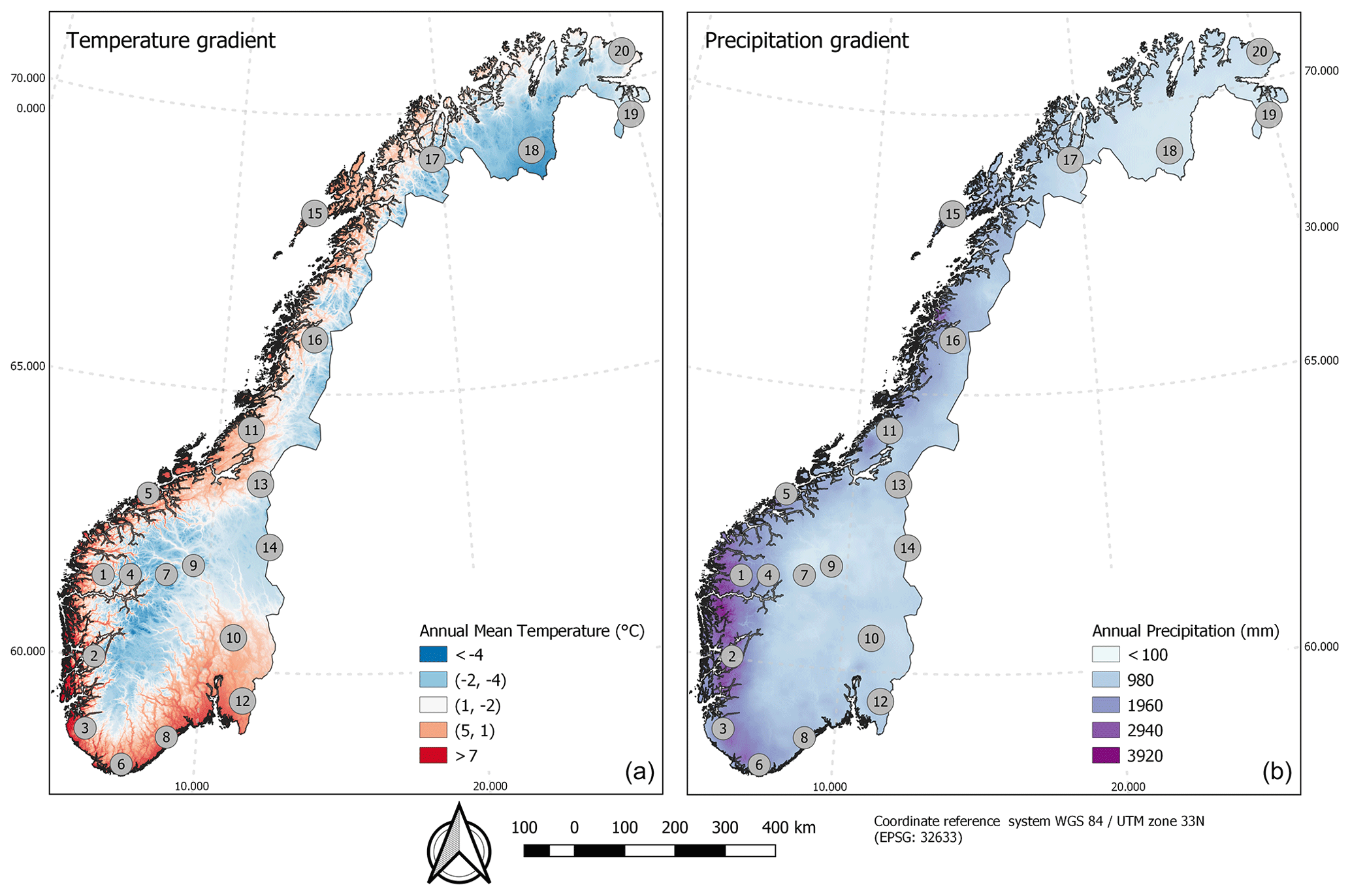
Figure 1 Locations of the 20 plots across the two main bioclimatic gradients in the study area: temperature (a) and precipitation (b). The plots are numbered by longitude from west to east. Exact values of temperature, precipitation and altitude for each plot are given in Table S1.

The vegetation of Norway is structured along two main bioclimatic gradients (Fig. 1), one related to temperature and growing-season length and one to humidity and oceanity (Bakkestuen et al., 2008). Broadleaf deciduous forests, regularly found in the southern and southwestern parts (the boreonemoral bioclimatic zone), are further west and north (in the southern boreal zone), restricted to locally warm sites (Moen, 1999). With declining temperatures northwards and towards higher altitudes, evergreen coniferous boreal forests dominate in the southern and middle boreal zones. In the northern boreal zone, the coniferous boreal forests pass gradually into subalpine birch forests, which form the tree line in Norway. A total of about 38 % of mainland Norway is covered by forests, and about 37 % of the land is situated above the forest line (of which two-thirds is covered by alpine mountain heaths). Wetlands cover approximately 9 %, and broadleaf deciduous forests cover about 0.4 % of the land area (Bryn et al., 2018).

2.2 The AR reference dataset

Data obtained by in situ field mapping, which is considered among the most reliable sources of land-cover information (Alexander and Millington, 2000), are practically and economically impossible to obtain in a wall-to-wall format for large land areas such as countries (Ullerud et al., 2020). As an alternative, area-frame surveys based upon stratified statistical sampling may provide accurate, area-representative, homogeneous and unbiased land-cover and land-use data for large areas. To evaluate the three methods for representing vegetation addressed in this study, we used the “Norwegian land cover and land resource survey of the outfields” (“Arealregnskap for utmark”) dataset (Strand, 2013), a Norwegian implementation of the mapping programme LUCAS (Land Use and Coverage Area frame Survey; Eurostat, 2003). Data were collected in the period between 2004 and 2014 in a systematic regular grid covering the whole land area of Norway, on which the plots (in total 1081 plots, each 0.6 km×1.5 km, i.e. 0.9 km²) were placed every 18 km (in latitude) by 18 km (in longitude) (Bryn et al., 2018; Strand, 2013). In each plot, expert field surveyors performed land-cover mapping by use of a system with 57 land-cover and vegetation-type classes (Bryn et al., 2018), mapped at a scale of 1:25 000. The data were provided in vector format with vegetation-type attributes assigned to each mapped polygon.

2.3 Study plots

Out of the 1081 rectangular AR plots, 20 were selected to make up our reference dataset, AR (Fig. 1; centre coordinates in Table S1 in the Supplement). The AR plots spanned elevations from 88 to 1670 m a.s.l., with mean annual temperatures between −4.0 and 7.1 ^∘C and mean annual precipitation between 466 and 2661 mm (Table S1). The gradients of precipitation and temperature are known to be among the most influential for vegetation distribution (e.g. Ahti et al., 1968; Bakkestuen et al., 2008). A series of Kolmogorov–Smirnov tests for comparison of sample mean and variance for these two variables using data from seNorge2 (Lussana et al., 2018a, b) was obtained to investigate if the 20 selected plots capture the variation across temperature and precipitation in Norway acceptably well compared to the full set of 1081 AR plots (Fig. S2). Additionally, we tested the representativeness across the range of variation for a third variable (precipitation seasonality) which was later selected for sensitivity experiments (see further details in Sect. 4). While low values of temperature and precipitation are slightly underrepresented in the 20 plots, the total range of variation was well covered. None of the tests for temperature, precipitation and the additional variable (precipitation seasonality) indicate that the sample of the 20 plots deviates from the full set of 1081 plots. The representativeness of the 20 plots was also tested against the full dataset of 1081 AR plots with regard to PFT coverage (in the Supplement, Sect. S3 and Table S3), using a chi-square test. This test showed that the two datasets are not more dissimilar than expected by chance.

2.4 Methods for representing vegetation

In this study, we use “plot” as a collective term for two partly overlapping spatial units: (i) the 0.9 km² rectangles of the AR reference dataset and (ii) the 1 km² quadrats with the same centre point as, and edges parallel to those of, the AR rectangles. The latter were used for the three methods of DGVM, RS and DM (Fig. S6).

Table 1 Details of each of the methods for representing vegetation. DGVM – dynamic global vegetation model, RS – remote sensing and DM – distribution model. PFT – plant functional type and VT – vegetation type.

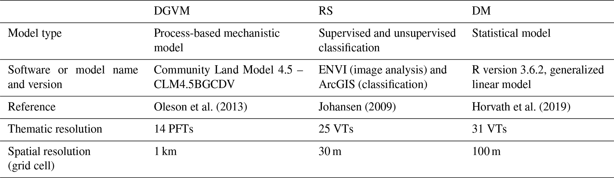
Representations of the present-day vegetation for each of these 20 plots were obtained by three different methods: (i) as the result of single-cell DGVM simulations for each plot, (ii) inferred from a RS vegetation map of the study area and (iii) from vegetation-type DM models (Table 1). In order to make the three methods comparable, vegetation was represented by plant functional type profiles (PFT profiles), obtained by a conversion scheme (Table S5 and Sect. 2.5). We define a PFT profile as a thematic representation of the land surface in a given plot or a group of plots, described as a vector of relative PFT abundances, i.e. values that sum up to one.

2.4.1 The DGVM method

The DGVM employed in this study was the CLM4.5BGCDV (hereafter referred to as DGVM), an option provided in NCAR's (National Center for Atmospheric Research) Community Land Model version 4.5 (CLM4.5) with vegetation dynamics, the plant–soil carbon–nitrogen cycle and multi-layer vertical soil enabled (Oleson et al., 2013). In DGVM, plant photosynthesis, stomatal conductance, carbon–nitrogen allocation, plant phenology and multi-layer soil biogeochemistry are described in accordance with default CLM4.5 values, while vegetation dynamics (establishment, survival, mortality and light competition) are handled separately based upon simple assumptions of environmental thresholds for establishment, survival and mortality of each PFT (see Sect. S7) (Oleson et al., 2013). We used DGVM in the form of single-cell simulations for the 20 plots with the grid-cell size set to 1 km×1 km (Table 1) to simulate the fractional cover of each PFT. All models were run with default CLM4.5 values for surface parameters (e.g. soil texture and depth), with prescribed atmospheric forcing derived from the 3-hourly hindcast of the regional model (SMHI-RCA4; Swedish Meteorological and Hydrological Institute Rossby Centre regional atmospheric model) driven by the ERA-Interim reanalysis for the European Domain of the Coordinated Downscaling Experiment (CORDEX) for 1980–2010 (Dyrrdal et al., 2018). The CORDEX model simulation was used because it has a higher spatial resolution than the default atmospheric forcing used in CLM4.5 ($\mathrm{0.11}{}^{\circ }\times \mathrm{0.11}{}^{\circ }$ and $\mathrm{0.5}{}^{\circ }\times \mathrm{0.5}{}^{\circ }$, respectively). An inspection of the choice of atmospheric forcing, by which the CORDEX data were compared with the seNorge data used for DM, showed minimal differences (Fig. S4). Only results obtained using CORDEX data are therefore shown in this paper. The 30-year CORDEX data were cycled during the spin-up. A 30-year period is consistent with WMO (World Meteorological Organization) climatological normal based on the rationale that a 30-year period is short enough to avoid large long-term trends while being long enough to include the range of variability. Thus, the data are not detrended or averaged.

The model was run with default PFT parameters (Table S7). All the selected sites are mostly undisturbed. In our experiments, soil C and N were firstly initialized using a restart file from an existing global present-day spin-up simulation with prescribed vegetation. Each model simulation was spun up for 400 years to establish a vegetation in equilibrium with the current climate after initialization from bare ground. In three plots where the equilibrium of vegetation was questionable (plot 6, 12 and 17), we extended the spin-up by 400, 200 and 200 years, respectively, to check if any effect on PFT profile could be seen. No significant changes in the PFT profile was noted in these three instances (Figs. S11.1 and S11.2), and therefore we kept the initial 400-year spin-up for all the sites. A 20-year average at the end of the spin-up was used as input for calculation of PFT profiles (representing years 1990–2010), which corresponds with the data-collection timeframe of the DM, RS and AR methods.

Among the 15 PFTs used in CLM4.5 to represent vegetated surfaces globally (Lawrence and Chase, 2007), only six (plus bare ground) were relevant for our study area (Table S7). Bare ground was predicted to occur where plant productivity was below a threshold value (Dallmeyer et al., 2019). The DGVM simulates the vegetated land unit only (non-grey boxes in Fig. S8), while other land units within the 20 plots, including glaciers, wetlands, lakes, cultivated land and urban areas, make up the excluded (EXCL) PFT category (Table S5). The percentage cover fraction of each PFT is equal to the average individual's fraction projective cover (FPCind) multiplied by the number of individuals (Nind) and average individual's crown area (CROWNind). FPCind is a function of the maximum leaf carbon achieved in 1 year, while CROWNind is related to dead stem carbon simulated by the model. Nind is mainly determined by the establishment and survival rate controlled by establishment and survival threshold conditions (Levis et al., 2004). We obtained PFT profiles for each plot by excluding the EXCL category and recalculated fractions of the vegetated land unit covered by each PFT to sum up to one.

2.4.2 The RS method

As a RS product we used SatVeg (Johansen, 2009), a vegetation map for Norway with 25 land-cover classes and a spatial resolution (grid-cell size) of 30 m (Table 1). SatVeg is obtained by a combination of unsupervised and supervised classification methods, applied to Landsat 5 TM (Thematic Mapper) and Landsat 7 ETM+ (Enhanced Thematic Mapper) images within the near-infrared and mid-infrared spectrum covering the period 1999–2006. While with the supervised classification, training data are based on well-labelled data from the study area, during the unsupervised classification the algorithm is only supplied with the number of output classes without further interference of the user. Only grid cells that were within each 1 km² plot with a majority of their area were taken into consideration for further calculations.

2.4.3 The DM method

The distribution models (DMs) for 31 vegetation types (VTs) obtained by Horvath et al. (2019) using generalized linear models (GLMs, with logit link and binomial errors, i.e. logistic regression) were used for this study. The VT data were collected during years 2004–2014. The DMs were obtained by using wall-to-wall data for 116 environmental predictors from six groups (topographic, geological, proximity, climatic, snow and land cover), gridded to a spatial resolution of 100 m×100 m (Table 1) as predictors. Important predictors were selected by an automated stepwise forward-selection procedure for each of the 31 VTs individually; thus each final model is built upon only a narrow selection of important predictors (Horvath et al., 2019). All DMs were evaluated using an independent evaluation dataset and by calculating the area under the receiver operator curve (AUC), a threshold-independent measure of model performance commonly used in DM (see Horvath et al., 2019, for details). AUC can be interpreted as the probability that the model predicts a higher suitability value for a random-presence grid cell than for a random-absence grid cell (Fielding and Bell, 1997). A seamless vegetation map (i.e. with one predicted VT for each grid cell with no overlap and no gaps) was obtained from the stack of 31 probability surfaces by assigning to each grid cell the VT with the highest predicted probability of occurrence within that cell (Ferrier et al., 2002). Grid cells with the majority of their area within a 1 km² plot were used for further calculations (Fig. S6).

2.5 Conversion to PFT profiles

Harmonization of the various vegetation classification systems was accomplished by a conversion scheme that represented each grid cell (RS and DM) or polygon (AR) in each of the 20 plots with one out of the six PFTs recognized by DGVM (Table S5 and Fig. S6). The scheme was obtained by expert judgements and solicited by a consensus process which involved ecologists participating in the AR survey as well as scientists working with RS and DGVMs.

We used the conversion scheme of Table S5 to generate wall-to-wall PFT maps from the original RS, DM and AR datasets (Table 1) by assigning one PFT to each 30 m×30 m grid cell, 100 m×100 m grid cell or VT polygon, respectively. PFT profiles for each plot, at the same thematic resolution as for DGVM, were obtained as the vector with fractions of grid cells or polygons assigned to each of the six PFTs. EXCL classes not represented in DGVM (cf. Table S5) were left out to minimize the effect of land use, which could otherwise have brought about differences in PFT profiles among the compared methods. PFT profiles were obtained for each combination of method and plot. To test for deviations in PFT coverage between the methods across the whole study area, aggregated PFT profiles were obtained by averaging the 20 PFT profiles obtained for each method.

2.6 Comparison of PFT profiles

To examine the overall pattern across the study area and to assess the models' ability to produce overall predictions of PFTs that accord with the PFTs' overall frequency (as given by the reference), aggregated PFT profiles obtained by each of the DGVM, RS and DM methods were compared with the aggregated PFT profile of the AR reference dataset by a chi-square test (Zuur et al., 2007). To identify strongly deviating modelling results at a plot scale, the dissimilarity between PFTs profiles obtained by each of the DGVM, RS and DM methods and the PFT profile of the AR dataset for each plot was calculated by using proportional dissimilarity (Czekanowski, 1909):

$$\begin{array}{ll}{\displaystyle }{d}_{hj}& {\displaystyle }=\sum |y_{hji}-y_{\mathrm{0}ji}|/\sum (y_{hji}+y_{\mathrm{0}ji})\\ \text{(1)}& {\displaystyle }& {\displaystyle }=\mathrm{1}-\mathrm{2}\sum min(y_{hji},y_{\mathrm{0}ji})/\sum (y_{hji}+y_{\mathrm{0}ji}),\end{array}$$

where y_hji refers to the specific element in a PFT profile vector (the fraction occupied by the PFT in question) given by method h (DGVM, RS or DM; $h=\mathrm{1},\mathrm{\dots },\mathrm{3}$; the value h=0 refers to the AR reference dataset), j refers to the specific plot ($j=\mathrm{1},\mathrm{\dots },\mathrm{20}$) and i refers to the PFT ($i=\mathrm{1},\mathrm{\dots },\mathrm{6}$). Proportional dissimilarity is the Manhattan measure standardized by division by the sum of the pairwise sums of variable values (here PFTs). Since the values of each PFT profile sums to one, the index reduces to

$${\displaystyle }{d}_{hj}=\mathrm{1}-\sum min(y_{hji},y_{\mathrm{0}ji}).$$

The proportional-dissimilarity index is appropriate for incidence data like PFT abundances, i.e. variables that take zero or positive values. The index reaches a maximum value of one when two objects have no common presences (here, PFTs present in both compared objects) and ignore joint absences (zeros). To assess the degree to which the models produce pairwise similar differences, we compared the pairwise differences between the proportional-dissimilarity values among methods using a Wilcoxon–Mann–Whitney paired-samples test.

All raster and vector operations related to the DM, RS and AR methods were carried out in R (version 3.4.3) (R Core Team, 2019) using packages “rgdal” (Rowlingson, 2019), “raster” (Hijmans, 2019) and “sp” (Pebesma and Bivand, 2005), while graphics are produced using the “ggplot2” package (Wickham, 2016). Statistical analyses were carried out in R (version 3.4.3) using the “vegan” package (Oksanen et al., 2019). All maps were produced in QGIS (QGIS Development Team, 2019).

3 Results

The aggregated PFT profiles for the RS and DM datasets did not differ significantly from those of the reference AR dataset according to the chi-square test, while a significant difference was found for the DGVM profiles (Table 2). While the proportion of grid cells attributed to the PFT boreal NET (boreal needleleaf evergreen tree) by the RS and DM methods underestimated AR values by 3.0 and 2.8 percentage points, respectively, DGVM overestimated the proportion of boreal NET by 20.4 percentage points compared to the AR reference. Also, unproductive areas (BG; bare ground) were overestimated by DGVM (by 16.6 percentage points) and less so by RS (4.0 percentage points), while this PFT was slightly underrepresented by DM (by 5.0 percentage points). Discrepancies were also observed for the cover of the C₃ PFT, which was overestimated by RS and DM (by 7.2 and 2.9 percentage points, respectively) and underestimated by DGVM (by 3.0 percentage points). Furthermore, DGVM overestimated BG and temperate BDT (broadleaf deciduous tree) cover on the expense of boreal BDT and boreal BDS (boreal broadleaf deciduous shrub).

Table 2 PFT profiles (columns) aggregated across all 20 plots for the three methods compared in this study and the AR reference dataset. Results of comparisons of aggregated PFT profiles for each of the three methods with the reference are also given. DGVM – dynamic global vegetation model, RS – remote sensing, DM – distribution model and AR – reference dataset. BG – bare ground, boreal NET – boreal needleleaf evergreen trees, temperate BDT – temperate broadleaf deciduous trees, boreal BDT – boreal broadleaf deciduous trees, boreal BDS – boreal broadleaf deciduous shrubs and C₃ – C₃ grasses.

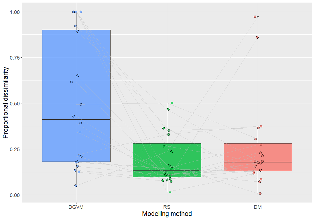
Figure 2 Proportional-dissimilarity values between PFT profiles for each combination of 20 plots and each of the three methods compared in this study and the corresponding plot in the AR reference dataset. The thick horizontal line, the box and the whiskers represent the median, the interquartile difference and the range of values for each method.

In accordance with results from comparisons between aggregated PFT profiles obtained by the three methods and those obtained for the reference dataset, DGVM profiles for individual plots were significantly more dissimilar to the AR reference than RS and DM profiles (Fig. 2). While RS had the lowest median proportional dissimilarity with the AR reference (0.19, compared to 0.26 for DM and 0.41 for DGVM), DM had the lowest spread of dissimilarity values, measured as interquartile difference (0.12, compared to 0.19 for RS and 0.72 for DGVM), among the three methods (Fig. 2). While no dissimilarity value for RS was above 0.50, two plots (4 and 19) acted as strong outliers in the distribution of DM values (cf. Fig. 2). Additionally, a comparison of proportional dissimilarity between pairs of methods revealed significant differences between DGVM profiles and those obtained by RS and DM (Wilcoxon rank-sum tests: W=111, p=0.0167 and W=88, p=0.0026, respectively), while RS and DM profiles were not significantly different from each other (Wilcoxon rank-sum test: W=161, p=0.3013).

Figure 3 PFT profiles for each of the 20 plots for the three methods compared in this study and the AR reference dataset. The columns in each cluster of the four bar charts represent, from left to right, the methods of the dynamic global vegetation model (DGVM), remote sensing (RS) and distribution model (DM), with the AR reference dataset to the right.

Visual inspection of spatial patterns of PFT profile characteristics across the 20 plots suggests that the best agreement among the methods was obtained for the southeastern part of the study area, dominated by boreal NET (Fig. 3 and Table S10). Compared to the AR reference dataset, PFT profiles obtained by DGVM were strongly biased: in the north (plots 17 and 18) towards boreal NET on the cost of boreal BDT, near the western coast (plots 1, 2, 5 and 15) towards boreal NET on the cost of boreal BDS and in southern coastal areas (plots 3, 6 and 12) towards temperate BDT instead of boreal NET. In plots 13 and 16 DGVM failed to establish vegetation (predicting bare ground) where AR reported boreal BDS. RS represented the PFT profiles of the AR reference well in most cases but tended to overestimate the frequency of dominance by C₃ grasses at several locations (plots 3, 16 and 20). While DM showed no general spatial pattern of PFT profile deviations from the reference dataset, PFT profiles of plots 4 and 19 obtained by DM had almost no similarity to the corresponding profiles of the AR reference dataset: C₃ grasses and boreal BDT were predicted instead of bare ground and boreal NET, respectively.

4 Sensitivity experiments and model improvement

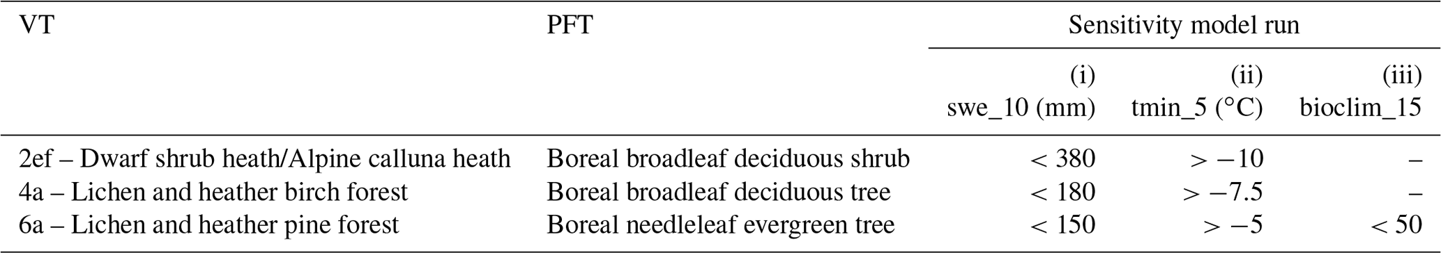
We used the results of PFT profile comparisons between DGVM and the AR reference (Fig. 3) and the results obtained for the DM dataset as a starting point for exploring the possible causes of the poor performance of DGVM. We first identified the three most abundant PFTs (i.e. boreal NET, boreal BDT and boreal BDS) in our set of plots (Table S3). Thereafter, we identified the major VTs predicted by DM in those plots that were translated into these PFTs using the conversion scheme (Table S5) (pine forest, birch forest and dwarf shrub heath, respectively; Table 3). Based on the results from Horvath et al. (2019), the corresponding final models for these three VTs were examined to identify important environmental variables that were driving the distribution of the VTs but not represented in DGVM. We recognized three environmental predictors that are critical for the distribution of each of these VTs and exhibit a clear threshold signature in the frequency-of-presence plots (i.e. graphs showing variation in the abundance of the VT as a function of an environmental predictors; also see Fig. S12): snow water equivalent in October (swe_10), minimum temperature in May (tmin_5) and precipitation seasonality (bioclim_15). Precipitation seasonality is defined as the ratio of the standard deviation of the monthly total precipitation to the mean monthly total precipitation (i.e. the coefficient of variation), expressed as a percentage (O'Donnell and Ignizio, 2012). Based on visual inspection of the frequency-of-presence plots, we identified specific threshold values for each of the three VTs (see Fig. S12 for details) and implemented these threshold values into DGVM as new limits for establishment of the three PFTs as shown in Table 3. For example, in line with Fig. S12, VT 2ef and its respective PFT, boreal BDS, can only establish when variable swe_10 is less than 380 mm.

Table 3 New thresholds for establishment of the three PFTs explored in DGVM sensitivity experiments. The variables explored were swe_10 – snow water equivalent in October given in mm, tmin_5 – minimum temperature in May (^∘C) and bioclim_15 – precipitation seasonality (unitless index representing annual trends in precipitation).

We explored the extent to which these additional thresholds improved the performance of DGVM on the subset of six plots (i.e. 1, 2, 5, 15, 17 and 18) in which the PFT profiles are most biased compared to the AR reference dataset due to the overrepresentation of boreal NEB. In total, three sensitivity experiments were carried out by a stepwise process; in each step a new threshold was added cumulatively to the previous experiment (Table 3). Namely, in the first sensitivity experiment (i), we added the swe_10 threshold. In the second experiment (ii), we added both swe_10 and tmin_5 as the threshold. In the last experiment (iii), we added all the three novel thresholds. Only the results of the third sensitivity experiment with all the three thresholds added are reported here. Results of the other two experiments are summarized in Table S13.

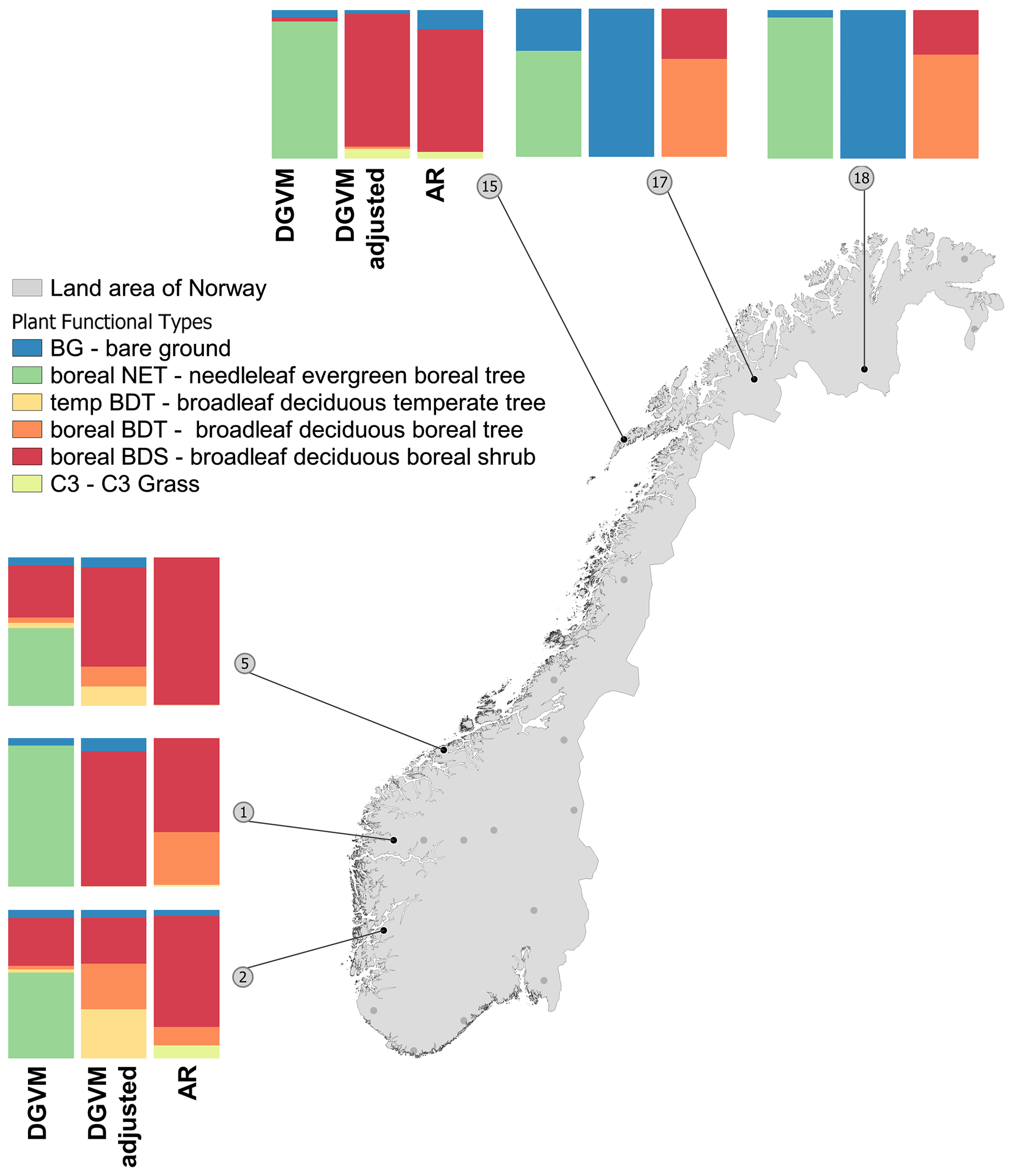
Figure 4 PFT profiles for the subset of six plots subjected to sensitivity experiments with new DGVM establishment thresholds. The columns in each cluster of the three bar charts represent, from left to right, the dynamic global vegetation model (DGVM) with original (default) parameter settings, DGVM with revised parameter settings and AR reference dataset. For further details, see Table S13.

The results show that while the added thresholds for swe_10 and tmin_5 had little impact on the results (Table S13), the addition of the threshold for bioclim_15 (i.e. the third sensitivity experiment) largely improved the performance of DGVM on the experimental plots explored (Fig. 4). PFT profiles simulated by this experiment were more similar to those of the AR reference dataset for four out of the six plots in the experimental subset (plot 1, 2, 5 and 15): in plots 1 and 15, boreal NET was correctly replaced by boreal BDS; in plots 2 and 5, boreal NET was replaced by boreal BDT, BDS and temperate BDT. The addition of new threshold (bioclim_15) also reduced the modelled abundance of boreal NET in plots 17 and 18, but DGVM still failed to populate these plots with another PFT (Fig. 4).

5 Discussion

5.1 Comparison of PFT profiles

The maps of PFT distributions generated by DM and RS are generally similar (Fig. S9) across most of our study area. This indicates that output from DM, which is rarely used for evaluating PFT distributions from DGVMs, can be used for this purpose in addition to the commonly used RS-based datasets. There are, however, some differences between results obtained by the two methods near the northern Norwegian coast and in the mountain areas of western Norway, which will be discussed below in more detail.

We recognize six possible explanations for the differences in PFT profiles obtained by DGVM, RS and DM for the 20 plots (see Table 4), related to the following issues: (i) the conversion scheme (ref. Table S5); (ii) what is actually modelled by DGVM, RS and DM, e.g. in terms of potential vs. actual vegetation; (iii) the performance of individual DM models; (iv) the transformation of predictions from single DMs into a seamless vegetation map, i.e. assigning one VT to each grid cell; (v) the DGVM performance; and (vi) missing PFTs in DGVM.

5.1.1 The conversion scheme

The conversion schemes used to reclassify vegetation and land-cover classes into PFTs have been reported as a possible attributor to erroneous PFT distributions (Hartley et al., 2017). While we use a simple conversion scheme that assigns each land-cover type or vegetation type to one and only one PFT (Dallmeyer et al., 2019), more complex conversion schemes exist, by which each land-cover class is translated into a multi-PFT composition that co-occurs within a grid cell (Bonan et al., 2002; Li et al., 2016; Poulter et al., 2011, 2015). Our approach may be advantageous when the classes to be converted are homogeneous, in the sense that one PFT is clearly dominating in the type and in the sense that the range of variation within the class in PFTs is negligible, such as is the case for 90 % of the DM and RS classes in our study. Our simple scheme may, on the other hand, be a source of uncertainty when quantitatively important VTs are ambiguous in one way or the other or, more commonly, in both ways at the same time. The set of VTs used in our study includes several relevant examples: VTs that may include a wide spectrum of tree-dominant types; the VT “1a/1b – Moss snowbed/Sedge and grass snowbed” (Horvath et al., 2019), which covers a range of variation in the relative abundance of graminoids and, hence, shows affinity to C₃ as well as to BG; and the VT “8a – Damp forest”, which is usually dominated by the evergreen Scots pine and converted into boreal NET, but which in some instances (e.g. after clear-cutting) is dominated by deciduous trees like Betula spp. and should then be converted into boreal BDT (Bryn et al., 2018). However, a close inspection of DM shows that our method reproduced similar PFT profiles as the reference dataset for all plots, except 2 out of 20 plots (the two outliers on Fig. 2, plots 4 and 19 in Fig. 3).

In our case, a more complicated conversion scheme is likely to be compensated for by the sub-grid complexity introduced in the process by which PFT profiles are obtained. Rather than estimating a PFT profile for the 1 km² plot directly, i.e. in one operation as in DGVM, the RS-based classes and VTs are first converted into PFTs in their original resolution and then subsequently subjected to aggregation to obtain the PFT profiles. This results in a sub-grid PFT heterogeneity that could otherwise be implemented by using a more complex conversion scheme.

5.1.2 What is modelled by DGVM, RS and DM

The methods used in this study produce different representations of the vegetated land surface in terms of actual or potential natural vegetation (Table 4). In order to model future vegetation changes and feedbacks, functional-type-based models like DGVM implicitly address the processes that control the distribution of vegetation (Bonan et al., 2003; Song et al., 2013). Simulating natural vegetation processes under a given climatic equilibrium scenario (at any given time), DGVM produces a model of potential natural vegetation (e.g. Bohn et al., 2000; Hengl et al., 2018). RS-based classifications, on the other hand, describe the land surface at a specific point in time or changes through time (e.g. Arctic greening and browning) (Myers-Smith et al., 2020) and, accordingly, portray actual vegetation as influenced by previous and ongoing land use (Bryn et al., 2013). Depending on the modelling setup, DM may pragmatically describe the current ecological envelope of a target or aim at revealing the proximate causes for its distribution (Ferrier and Guisan, 2006), thus modelling either actual or potential natural vegetation, depending on the input data used for modelling (Hemsing and Bryn, 2012; Hengl et al., 2018).

Table 4 A summary of the key properties of the three methods compared in this study. DGVM – dynamic global vegetation model, RS – remote sensing and DM – distribution model.

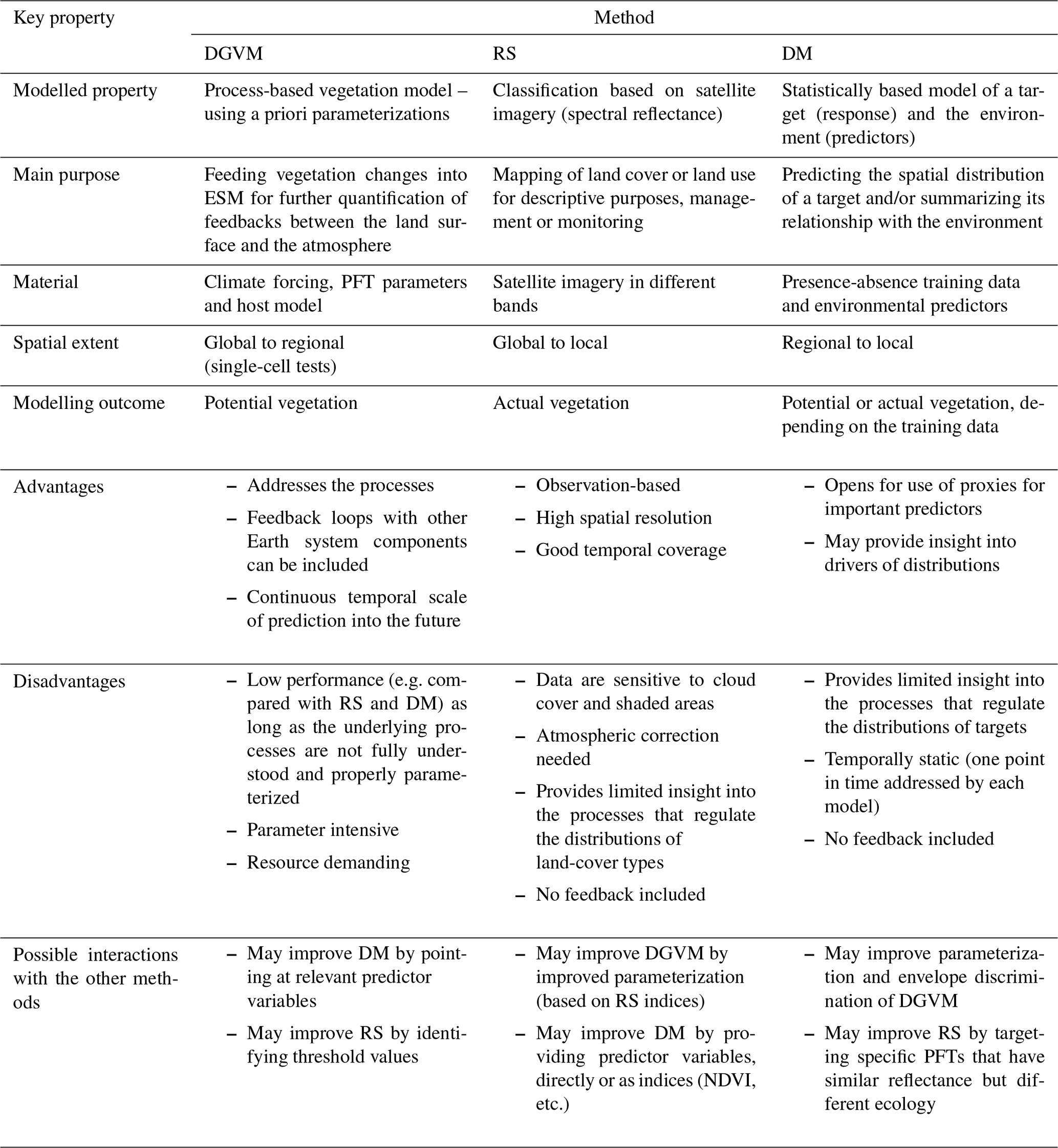
In this study, we carefully restricted our attention to PFTs that represent natural vegetation, excluding VTs with strong anthropogenic influences. This was done for all methods and the AR reference. Nevertheless, differences with respect to what is actually modelled by the different methods, potential vegetation by DGVM and actual vegetation by RS and DM, may have contributed to the observed among-model differences in PFT profiles.

5.1.3 DM performance

While the performance of the DM method is overall good, distribution models of individual VTs vary in performance (with AUC values ranging from 0.671 to 0.989) according to the study by Horvath et al. (2019). Several reasons for the low predictive performance of some DM runs are identified, of which the most important is considered to be important predictors missing in the training data. This might seem counter-intuitive, given the large number of predictor variables used in the study (n=116). However, the authors conclude that several important factors for the distribution of vegetation are not at all represented in the dataset (e.g. NDVI and lidar), among other reasons because they are almost impossible to obtain data for with the required spatial resolution (e.g. soil nutrients). The DM method requires estimates for the probabilities of occurrence for (almost) all individual vegetation types to create a seamless vegetation map, which in turn is required for making estimates for the PFT profiles as robust as possible. Thus, in this context, “poor” models are better than no model.

Individual models' performance might be the reason for the two plots whose PFT profiles deviate strongly from the AR reference (Figs. 2 and 3). For plot 4, the discrepancy is due to VT 1a/1b – Moss snowbed/Sedge and grass snowbed, which is represented by one of the best performing among the 31 DMs. For this VT, conversion scheme bias is a more likely reason for the deviant PFT profile. For plot 19, boreal BDT is modelled because the VT predicted by DM is “4a – Lichen and heather birch forest”. The fact that the DM for this VT is among the inferior DMs (see the ranking of individual models presented in Horvath et al., 2019) makes this explanation more likely in this case.

5.1.4 Transformation of single-DM predictions into a vegetation map

The performance of DM on the particular plots may also be influenced by the method chosen for transforming predictions from one DM for each VT into a seamless vegetation map. Assigning to each grid cell the VT with the highest predicted probability of presence in that cell, which is a commonly used method for this purpose (Ferrier and Guisan, 2006), favours VTs represented by good DMs. This is brought about by good DMs having a distribution of predictions that is more spread out (with larger predictions for the grid cells identified as the most favourable cells) than poor DMs (Halvorsen, 2012). However, since the probability of presence for each VT was predicted separately for each grid cell, the probability values for each VT vary independently of the probabilities for the other VTs, throughout the study area. Thus, we regard the chance that one VT consistently outperforms another VT over all the grid cells to be negligible. Alternative methods for this purpose should be tested in the context of DGVM evaluation. To avoid uncertainties associated with conversion between type systems and perhaps even further improve the performance of DM, we recommend exploring the option of using PFTs directly as targets in DM. Direct modelling of PFTs rather than taking the detour via VT models may reduce the number of environment predictors required (116 layers used in Horvath et al., 2019) in addition to circumventing the complicated process of modelling thematically narrow vegetation types (VTs). Another potential advantage of modelling PFT targets directly is that the model parameters will then be PFT specific and not in need of being converted (from a VT into a PFT).

To further reduce the biases and uncertainties of DM-based PFT profiles, we recommend exploring the use of variables derived from RS directly as predictors in DM. Previous studies have shown that RS-based predictors may enhance DM performance on different scales: on the vegetation-type level (Álvarez-Martínez et al., 2018), on the habitat-type level (Mücher et al., 2009) and on the PFT level (Assal et al., 2015). Further suggestions for improvement of the methods used in this study are found in Table 4.

5.1.5 DGVM performance

Our results show that, for many plots, the PFT profiles simulated by DGVM differ from those of the AR reference dataset. According to our results, DGVM overestimates the coverage of bare ground and boreal NET and underpredicts the cover of C₃ grasses, boreal BDT and boreal BDS. While the AR reference dataset shows that the northern plots (specifically plots 17 and 18) are covered by mountain birch forest and shrubs (boreal BDT and boreal BDS), DGVM predicts dominance of boreal NET in these plots. Overestimation of boreal NET has also been reported by Hickler et al. (2012) for large parts of Scandinavia, who attributed this to lacking representation of shade tolerance classes in DGVM models. A similar pattern is seen in our results: the PFT profiles obtained by DGVM during the 400-year spin-up (Fig. S11.1) show no sign of boreal BDT in the early phases of model prediction, as would be expected of an early-successional forest in Norway.

Our results further suggest that DGVM underrepresents grasses and shrubs compared to the reference dataset. This may be explained by the built-in constraints in the light competition scheme of DGVM. The model assumes that regardless of grass and shrub productivity, trees will cover up to 95 % of the land unit when their productivity permits (Oleson et al., 2013). The priority given to a PFT in DGVM decreases with the stature of the organisms in question because of the increasing probability that a lower layer is covered by another layer. The degree of underrepresentation is therefore expected to increase from shrubs to grasses. Accordingly, DGVM predicts dominance by trees in the most productive regions, by grasses in less productive regions and by shrubs in the least productive non-desert regions (Zeng et al., 2008). The underrepresentation of C₃ grasses by DGVM across the 20 plots accords with the results of Zhu et al. (2018), who found that C₃ grasses are underpredicted on a global level in an earlier version of DGVM.

Inappropriate parameterization of shrubs may be a reason why the DGVM underestimates boreal BDS in many of the coastal plots (1, 2, 5 and 15) (Fig. 3 and Table S10). The implementation of shrubs as a new PFT in an earlier version of DGVM (CLM3-DGVM) by Zeng et al. (2008), parameterized for representation of taller shrubs with heights between 0.1 and 0.5 m, may not suit the majority of dwarf shrubs (of the genera Calluna, Betula and Empetrum) that abundantly occurs in Norwegian ecosystems. To this, Gotangco Castillo et al. (2012) add that the sparse shrub and grass vegetation cover simulated by DGVM in the tundra regions may be caused by the soil moisture bias inherited from the host land model CLM4 (Lawrence et al., 2011). Another reason for DGVM's underestimation of boreal BDS in coastal areas could be the 4000-year tradition of coastal heath management in Norway (Bryn et al., 2010) which causes a large discrepancy between the actual vegetation modelled by RS, DM and AR and the potential natural vegetation simulated by DGVM under present-day climatic conditions (e.g. Bohn et al., 2000; Hengl et al., 2018). We therefore argue that more sensitivity studies of PFT-specific parameters for height, survival, establishment, etc., across all PFTs, are needed.

Some discrepancies in the DGVM output might be caused by the climate forcing used in the simulations, looped for the period 1980–2010. Long-term historical climate effects on vegetation distribution were not included in our model simulation. However, we noticed that vegetation distribution was insensitive to interannual variation or decadal variation of the climate forcing when it reached an equilibrium state in most of our study sites. Even though long-term historical climate effects (such as cooler temperature in the early 20th century) may favour boreal BDS rather than boreal NET, we consider such historical effects to have only minor impact on the already large biases observed in DGVM (e.g. too much boreal NET and too few BDS). We also note that DGVM used a spatially coarser CORDEX reanalysis (11 km×11 km) to supply high-temporal-resolution (6-hourly) atmospheric forcing data, while the climate predictors used in DM were derived from the observation-based seNorge2 dataset with 1 km×1 km spatial resolution and daily temporal resolution. The larger biases in the CORDEX reanalysis data may also contribute to the large mismatch between DGVM and the reference dataset. We have compared the average annual temperature and annual precipitation of the two input datasets used in DGVM and DM to look for differences (see Fig. S4). It appears that precipitation estimates by CORDEX for the 20 plots were slightly higher than seNorge estimates; the converse (although less pronounced) was true for temperature. The consequences of these differences in the input data might be investigated in follow-up studies.

Despite the shortcomings discussed above, DGVM performs reasonably well for some PFTs. One example is the temperate BDT, which is correctly predicted by the model to be restricted to the southern coastal plots (Bohn et al., 2000; Moen, 1999). This finding suggests that some climatically driven PFTs (i.e. temperate BDT) are well implemented by the existing parameters in the DGVM used in this study.

5.1.6 Missing PFTs

DGVM coerces the world's immense variation in plant species composition (vegetation) into a very limited number of predefined PFTs, compared to classification schemes used by the other methods in this study (RS, DM and AR; see Table S5) and by other approaches to systematization of ecodiversity (e.g. Dinerstein et al., 2017; Keith et al., 2020). In particular, the number of high-latitude specific PFTs is insufficient to realistically represent the biodiversity of these ecoregions, as pointed out by Bjordal (2018) and Vowles and Björk (2017). Comparisons between PFT profiles obtained by DGVM and profiles obtained by DM suggest specific vegetation types that need to be better represented in DGVMs, either by improving an existing PFT or by adding a new PFT (e.g. dwarf shrubs vs. tall shrubs; moss-dominated snowbeds, wetlands and lichens). In our study, the PFT profile of DGVM is represented by the six boreal PFTs, whereas the original data for RS, DM and AR include an average of 17 % (ref. Table S3) of the total area that are not represented by these six PFTs (classes for the EXCL PFT category, see Table S5). This points to the missing PFTs in the classification scheme of DGVM but also to the challenge that certain ecosystems in our study area do not have a representation in the PFT schemes of DGVM. This is exemplified by wetlands, important ecosystems that are still not represented in many of the current DGVMs. This is not only problematic from the perspective of the land surface energy balance (Wullschleger et al., 2014) but has also implications for modelling of carbon storage and cycling and other interactions between the land surface and the atmosphere (Bjordal, 2018).

Some recent examples with improvements to the thematic resolution of PFTs in DGVMs are available in the literature (Druel et al., 2019, 2017; Coppell et al., 2019; Chadburn et al., 2015; Porada et al., 2016), and further examples of DGVMs with a larger number of high-latitude PFTs also exist (Euskirchen et al., 2009). In line with these studies, our results demonstrate a great potential for increasing the thematic resolution of DGVMs in general and not limited to the DGVM tested here, in terms of developing and parameterizing new specific PFTs to be representative of the highlatitude and high-altitude habitats and also deriving parameters from observations, DMs or RS products (Bjordal, 2018; Wullschleger et al., 2014), specific for the high latitudes (Druel et al., 2017).

5.2 Sensitivity experiments

Adjusting DGVM parameters so that they correspond better with environmental drivers known to be functional in the high-latitude PFTs has been suggested as a measure to improve the performance of DGVM (Wullschleger et al., 2014). Our sensitivity experiments demonstrate that DM results can inform DGVM parameterization based upon suitability ranges of the environmental predictors recognized by DM in determining the distribution of a PFT. Most notably, we recognize that the implementation of precipitation seasonality (bioclim_15<50) as a threshold for the establishment of NET, which has not yet been used in DGVM, improves the distribution of high-latitude PFTs simulated by DGVM. This adds to the environmental thresholds for the establishment of a PFT previously used in DGVMs to restrict the predicted distribution of PFTs to realistic geographic regions (Miller and Smith, 2012). Even though our sensitivity experiments focus on a limited number of additional thresholds across three PFTs, this approach shows promising results and is worth exploring more extensively in future studies.

The importance of precipitation seasonality (i.e. bioclim_15) as a critical limiting factor for the establishment of boreal NET indicates that the increased seasonality impedes growth of boreal NET. While some studies have emphasized the importance of seasonal distribution of rainfall on vegetation in the semi-arid areas (Zhang et al., 2018), the importance of this factor for high-altitude areas is less well studied (Oksanen, 1995; Sevanto et al., 2006). Better representation of the processes related to the response of boreal NET to water availability, especially spring drought in DGVM, also warrants further investigation. From our results for plots 17 and 18, we notice that adjusting the climatic thresholds for the establishment of boreal NET does not necessarily lead to other PFT growth. Boreal BDT and BDS can establish at both plots, but their growth rates are too slow to make them occupy a large area at these plots. This implies that other environmental conditions, e.g. nitrogen availability, might play a more important role in limiting the growth of BDT and BDS in the tested DGVM. The biases of DGVM in simulating BDT and BDS has been widely noticed in previous studies (Gotangco Castillo et al., 2012) and remains a challenge requiring more investigation in the future.

While going into further details of which additional PFTs should be included in DGVMs and how these and other PFTs should be parameterized is beyond the scope of the present paper, we emphasize the potential of using DM for improving the parameters of DGVMs. More specifically, we propose a more intensive exploration of DM as a tool for identification of potential environmental drivers for the high-latitude PFTs, which may enhance the performance of DGVMs in high-latitude ecoregions. The specific focus of our study is the boreal region, both because of the importance of these ecosystems in the climate system and because of the data availability of vegetation-type DM and the field-based reference dataset (AR). However, we believe that the improved DGVM parameters resulting from our sensitivity experiments may be applicable to other DGVMs such as Terrestrial Ecosystem Model (TEM) and LPJ-GUESS (Lund–Potsdam–Jena General Ecosystem Simulator) (Euskirchen et al., 2009; Miller and Smith, 2012). Also, the results from this study are likely to be transferable to other high-latitude areas in the circumboreal region.

6 Conclusions

This study demonstrates the potential of using distribution models (DMs) for representing present-day vegetation in evaluations of plant functional type (PFT) distributions simulated by dynamic global vegetation models (DGVMs) and for the improvement of specific PFT parameters within DGVMs. By the identification of the main differences among PFT profiles obtained by three methods (DGVM, RS and DM) in selected high-latitude plots distributed across climatic gradients in Norway, we show that PFT profiles derived from DM and RS are in the same range of reliability, judged by the resemblance to a reference dataset (AR). Hence, we suggest that DM results can be used as a complementary evaluation dataset to benchmark the present-day DGVMs. This approach is recommended when high-quality RS products are not available in the desired thematic resolution or when they are not able to supply proxies of other properties (such as deriving parameter improvements or PFT-specific traits).

Comparing the 20 PFT profiles obtained by DGVM with those obtained by AR shows a large overestimation by DGVM of boreal needleleaf evergreen trees (boreal NET) and bare ground at the expense of boreal broadleaf deciduous trees and shrubs. This is attributed to missing processes and PFT parameterizations of high-latitude PFTs in DGVM. We use DM results to identify a new PFT-specific environmental parameter – precipitation seasonality – which, in a series of sensitivity experiments, improves the distribution of boreal NET predicted by DGVM. This new PFT-specific threshold for establishment decreases the bias of boreal NET in DGVM across four out of six plots, and as a result, the distribution of other high-latitude PFTs is also better represented. We argue that this new threshold should be transferable to other DGVMs simulating high-latitude PFTs and that our DM-based approach can be well applied to other ecosystems.

Further development of DGVM, such as refining parameters for existing boreal PFTs and increasing the thematic resolution of PFTs for boreal areas, should be strongly encouraged to achieve a more realistic simulation of the distribution of vegetation by DGVM to increase the reliability of future predictions and the reliability of predicted vegetation feedbacks in the climate system.