the Creative Commons Attribution 4.0 License.
the Creative Commons Attribution 4.0 License.
 | 14 Apr 2022
New constraints on biological production and mixing processes in the South China Sea from triple isotope composition of dissolved oxygen
Hana Jurikova
Osamu Abe
Fuh-Kwo Shiah
The South China Sea (SCS) is the world's largest marginal sea, playing an important role in the regional biogeochemical cycling of carbon and oxygen. However, its overall metabolic balance, primary production rates and links to East Asian Monsoon forcing remain poorly constrained. Here, we report seasonal variations in triple oxygen isotope composition (17Δ) of dissolved O2, a tracer for biological O2, gross primary production (GP; inferred from δ17O and δ18O values) and net community production (NP; evaluated from oxygen–argon ratios) from the SouthEast Asian Time-series Study (SEATS) in the SCS. Our results suggest rather stable mixed-layer mean GP rates of ∼ 1500 ± 350 mg C m−2 d−1 and mean NP of ∼ −13 ± 20 mg C m−2 d−1 during the summer southwest monsoon season. These values indicate, within uncertainties and variabilities observed, that the metabolism of the system was in net balance. During months influenced by the stronger northeast monsoon forcing, the system appears to be more dynamic and with variable production rates, which may shift the metabolism to net autotrophy (with NP rates up to ∼ 140 mg C m−2 d−1). Furthermore, our data from the deeper regions show that the SCS circulation is strongly affected by monsoon wind forcing, with a larger part of the water column down to at least 400 m depth fully exchanged during a winter, suggesting the 17Δ of deep O2 as a valuable novel tracer for probing mixing processes. Altogether, our findings underscore the importance of monsoon intensity on shifting the carbon balance in this warm oligotrophic sea and on driving the regional circulation pattern.
- Article
(4893 KB) - Full-text XML
-
Supplement
(274 KB) - BibTeX
- EndNote


The South China Sea (SCS) is the largest marginal sea of the world and significantly influences the regional biogeochemistry and climate (Wong et al., 2007a). The SCS also contributes to global circulation. A pathway through the SCS connects the tropical Pacific with the Indian Ocean, impacting the Indonesian Throughflow, a current which plays a pivotal role in the coupled ocean and climate system (Qu et al., 2005). It has been suggested that marginal seas may act as a significant global atmospheric carbon dioxide (CO2) sink, primarily due to CO2 absorption by continental shelf waters (Tsunogai et al., 1999; Liu et al., 2000; Yool and Fasham, 2001; Chen et al., 2003; Thomas et al., 2004). However, the heterogenous nature together with latitudinal differences between ocean margins makes joint extrapolations to a global scale highly uncertain. Most observations have revealed that seas at mid-latitude shelves, which experience strong spring blooms and clear seasonal patterns, function particularly well as CO2 sinks (e.g. the North Sea, Frankignoulle and Borges, 2001; the Gulf of Biscay, Thomas et al., 2004; the Celtic Sea, Seguro et al., 2019; the East China Sea, Tsunogai et al., 1999; Wang et al., 2000; or the Mid-Atlantic Bight, DeGrandpre et al., 2002). Conversely, tropical and subtropical shelves and marginal seas are most likely CO2 sources (Cai and Dai, 2004), and a similar scenario may also be anticipated for the SCS. While several studies reaffirmed that the SCS indeed acts as a source of CO2 to the atmosphere in the spring, summer and autumn (Rehder and Suess, 2001; Zhai et al., 2005), Tseng et al. (2005) reported on the uptake of CO2 during winter from the SCS. The observed CO2 invasion, driven by an unusual seasonal pattern in the oligotrophic open northern part of the SCS with elevated chlorophyll concentrations (0.30–0.35 mg m−3) and primary production (300 mg C m−2 d−1), was apparently large enough to compensate for the CO2 evasion during the rest of the year, resulting in only minor net annual sea–atmosphere CO2 fluxes (0.24 g C m−2 yr−1; Tseng et al., 2007). Although the primary production and phytoplankton biomass are low for most of the year in the SCS, it appears that a clear winter maximum can be found regularly – a distinct seasonal pattern from other low-latitude water bodies. Clearly, the role of the SCS (and marginal seas in general) is complex, and their seasonal carbon cycling demands further study.
Owing to its geographical position between the Tibetan Plateau and the western Pacific warm pool, the SCS is continuously exposed to the East Asian Monsoon, which plays a fundamental role in its oceanography and biogeochemistry (see Wong et al., 2007a, for an overview). From June to September, the weaker southwest summer monsoon (SWM) drives the anti-cyclonic circulation gyre, while the strong northeast winter monsoon (NEM) propels a basin-wide cyclonic circulation gyre between November and April (Fig. 1). This intense seasonal reversal drives the short- and long-term physical, chemical and biological processes that control the distribution of phytoplankton communities (Ning et al., 2004). As a result, intermediate chlorophyll a (Chl a) concentrations are typically associated with the SWM, while the highest phytoplankton biomass is expected during the NEM due to increased diapycnal nutrient supply from the thermocline. Winter mean Chl a concentrations often peak at about 0.50 mg m−3 in the subsurface chlorophyll maximum and at 0.20 mg m−3 at the surface (Liu et al., 2002). Upwelling produced by the convergence of currents in the cyclonic gyre near Luzon Strait, where the Kuroshio intrudes, can at times enhance the mean Chl a concentration (to about 0.65 mg m−3) and primary production in winter to about 8 times the summer values (Chen et al., 2006). Conversely, lowest Chl a values have been observed during inter-monsoon seasons (Liu et al., 2002; Wong et al., 2007b; Li et al., 2017). Superimposed on the main seasonal monsoon-driven pattern, episodic events such as typhoons may temporarily elevate primary production due to wind-enhanced vertical mixing, bringing nutrients from the nutricline to the mixed layer and stimulating production. For instance, Lin et al. (2003) reported a bloom patch with average surface Chl a concentrations of 3.20 ± 4.40 mg m−3 during the passing of tropical cyclone Kai-Tak in July 2000. In addition to typhoons, the SCS has been suggested to be sensitive to various types of short-term physical forcings including tides, internal waves, eddies or topography–flow interactions (Lin et al., 2010; Tai et al., 2020; Lai et al., 2021). Generally, these tend to enhance vertical mixing, supplying nutrient-rich waters to the mixing layer, which enhance phytoplankton production and Chl a concentration (to about 0.30–0.40 mg m−3) in the oligotrophic waters of the SCS. Interannual variability in the SCS is primarily driven by the ENSO (El Niño–Southern Oscillation), which modulates the strength of the monsoon forcing, which in turn affects the regional marine biogeochemistry. During warm (cold) El Niño (La Niña) episodes in the Pacific, the monsoon tends to have a late (early) onset, and the monsoon intensity is generally weaker (stronger; Zhou and Chan, 2007). Consequently, weakened wind mixing and strengthened water column stratification results in anomalously low Chl a concentrations in the northern SCS. For example, the 1997–1998 El Niño event was one of the most powerful ENSO events in recorded history and caused concentration of surface Chl a to drop from 0.20 to 0.10 mg m−3 in the northern SCS and the mean winter production to be reduced by about 40 % (Shang et al., 2005; Tseng et al., 2009).
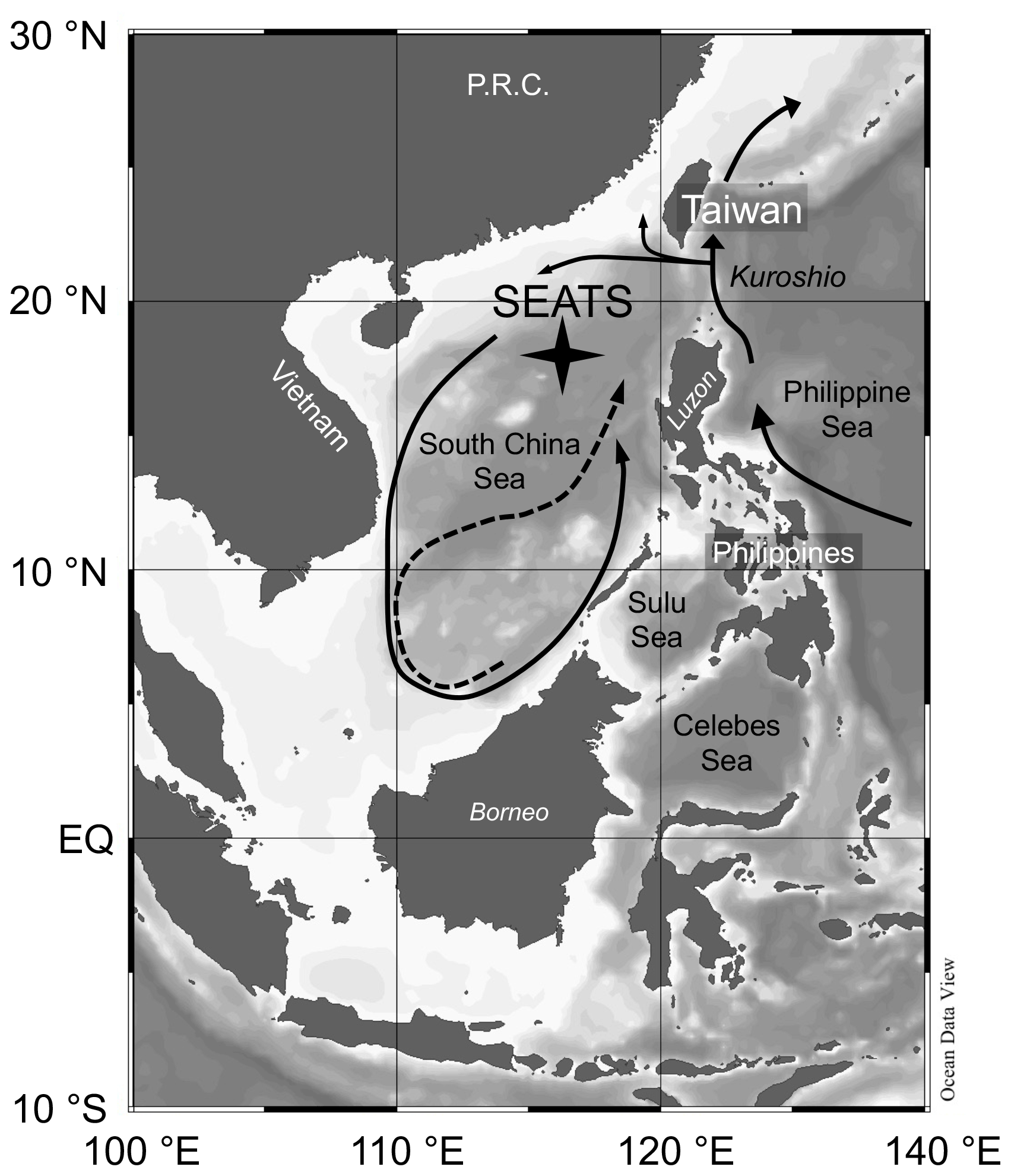
Figure 1Bathymetric map of South China Sea (SCS) and surrounding areas with position of the SouthEast Asian Time-series Study (station 55, SEATS) indicated. Arrows in the SCS indicate the circulation patterns – solid line shows the basin-wide cyclonic gyre during winter; dashed line represents the eastward jet off the Vietnam coast and the anticyclonic gyre over the southern half of the SCS throughout the summer. Map was created using Ocean Data View (https://odv.awi.de/, Schlitzer, 2020).
Accurate quantification of phytoplankton production rates, a fundamental property of the ocean system, remains a challenge primarily due to methodological biases. This has been a subject of increasing debate over the past years, resulting in augmented efforts to compare and resolve production rates through different methods (e.g. Juranek and Quay, 2013; Regaudie-de-Gioux et al., 2014). In the SCS and at the SouthEast Asian Time-series Study (SEATS; Wong et al., 2007a), our understanding of primary production is predominantly limited to opportunistic assessments using the 14C-assimilation method (Liu et al., 2002) or satellite-based SeaWiFS observations (Liu et al., 2002; Lin et al., 2003). While the traditional 14C approach (Steeman-Nielsen, 1952) is limited due to its in vitro nature, which cannot reflect the time-averaged mixed-layer phytoplankton production (Marra, 2002), the latter relies on calibrations against field measurements that are spatially and temporally scarce (Carr et al., 2006). Although not exempt of uncertainties (Juranek and Quay, 2013), as these are inherent to any productivity determination, the triple oxygen isotope composition (17Δ) technique (Luz et al., 1999; Luz and Barkan, 2000) combined with measurements has proved to be a powerful tool to provide a new perspective on evaluating primary production (e.g. Sarma et al., 2005; Reuer et al., 2007; Stanley et al., 2010; Hamme et al., 2012; Castro-Morales et al., 2013; Jurikova et al., 2016). The key advantage of this technique is that 17Δ allows for distinguishing photosynthetic O2 input from other sources directly in situ, while the co-variation of δ17O and δ18O, the “dual-delta approach” (Prokopenko et al., 2011; Kaiser, 2011), enables an estimation of the integrated gross productivity in the mixed layer.
In order to evaluate the photosynthetic O2 production and its contribution to the local carbon balance, as well as improve our understanding of seasonal variabilities in primary production in the SCS, we performed triple isotopic analyses and determined the ratio of dissolved O2 samples from five vertical profiles during the occupation of SEATS in October 2013, August 2014 and April 2015. We combined the 17Δ and the tracer data to study the seasonal trends in photosynthetic vs. atmospheric O2 input in the upper water column (∼ 200 m), which we relate to the main monsoon seasons. Gross and net primary production rates are also estimated and discussed. Finally, owing to the limited contribution from photosynthesis and air–sea gas exchange to the 17Δ signal in a parcel of deep water (200 to 3500 m), the potential for the application of the tracer for assessing mixing processes is discussed.
2.1 Sampling and analysis
Sampling was carried out aboard R/V Ocean Researcher-1 during cruises CR1053 (in October 2013), CR1084 (August 2014) and CR1103 (April 2015) at station 55 “SEATS” (SouthEast Asian Time-series Study; 18∘ N, 116∘ E; Fig. 1) in the South China Sea (SCS). Seawater was collected using a rosette sampler equipped with 20 L Niskin bottles attached to a Sea-Bird SBE 911Plus CTD (conductivity–temperature–depth). Samples for dissolved oxygen analysis were obtained on 16 October 2013 (11 depths: 5, 10, 30, 50, 80, 100, 150, 200, 300, 400 and 500 m), on 5 August 2014 (11 depths: 5, 10, 20, 80, 100, 200, 600, 1000, 1800, 2500 and 3500 m), on 6 August 2014 (13 depths: 5, 10, 20, 50, 80, 200, 400, 600, 1000, 1200, 1800, 2500 and 3500 m), on 24 April 2015 (14 depths: 5, 10, 20, 80, 100, 150, 200, 300, 400, 500, 600, 1000, 1800 and 3500 m) and on 25 April 2015 (7 depths: 5, 10, 20, 30, 50, 80 and 100 m; see also the Supplement).
The accuracy of dissolved oxygen concentration measurements from the CTD was verified and calibrated against in vitro measurements. Briefly, water samples were siphoned into triplicate 60 mL bottles (Wheaton), and the Winkler titration method by Pai et al. (1993) was adopted for in vitro dissolved O2 determination with a precision of 0.2 % r.s.d. (relative standard deviation; full scale). Concentrations of Chl a were measured by a fluorometer (Chelsea AquaTracka III) attached to the CTD to monitor vertical profiles of fluorescence and calibrated by in situ Chl a measurements with a Turner Designs fluorometer (10-AU-005) after extraction with 90 % acetone using a non-acidification method (Gong et al., 1996). The precision of Chl a measurements using a Turner fluorometer is usually better than 8 % for any chlorophyll values exceeding 0.50 mg m−3 (Strickland and Parsons, 1972), with any uncertainties in the estimation of Chl a linked to the presence of Chl b being below 5 % (Lorenzen, 1981). We compared two mixed-layer depth definitions: (1) temperature-based definition defined by 1 ∘C (ΔT) threshold from reference temperature value at 10 m depth, and (2) dissolved-O2-based definition defined by 1 % (ΔO2) threshold from reference O2 concentration at 10 m depth. Selected mixed-layer depths were further verified by careful visual inspection of vertical temperature, density and dissolved oxygen profiles. Although the preferred dissolved-O2-based mixed-layer definition considers a relative difference of 0.5 % O2 concentration to a reference value at 10 m (Castro-Morales and Kaiser, 2012), we did not find this definition suitable for our study location, as the oscillations in O2 concentration in the mixed layer alone were of the order of 0.5 %. Instead, we opted for the 1 % definition, which also closely agreed with the visual inspection of the profiles. The limit of the photic zone was defined as the depth where the photosynthetically active radiation (PAR) was 1 % of the surface value. We used Ocean Data View (ODV; Schlitzer, 2020) for profile visualization.
Triple oxygen isotope analyses were carried out at Academia Sinica, Taiwan. The triple oxygen isotope composition or 17O-excess (Luz et al., 1999; Luz and Barkan, 2000) is defined as
where the isotopic compositions δ17O and δ18O represent the deviation of the abundance ratio of an isotopic and normal species in a sample relative to that of a standard:
where ∗O is either 17O or 18O. Here, δ17O and δ18O are expressed with respect to atmospheric air O2, and following Luz and Barkan (2005) the factor λ is taken to be 0.518. As suggested by Luz and Barkan (2011), we note that a slope of λ=0.516 might present a more appropriate choice. However, in order to enable a direct comparison to other studies, we preferred the earlier value, which has been largely applied in studies on marine production to date. The use of a slope λ=0.516 would result in only a minor increase in 17Δ (about 1 %–8 % of the reported values), which for most of our samples remains within analytical uncertainties.
Our laboratory protocols for dissolved oxygen sample preparation and analysis are detailed in Jurikova et al. (2016). Note that O2–Ar data are not available for the profile from October 2013 due to the setting of the gas chromatograph condition at a dry-ice–acetone slush temperature for complete separation of O2. In summary, dissolved gases were extracted from water following Emerson et al. (1995) and Luz et al. (2002). δ17O and δ18O values of O2 in the purified oxygen–argon mixture (or pure oxygen for October 2013 samples) were determined by dual-inlet mass spectrometry (Thermo Scientific Finnigan MAT 253 isotope ratio mass spectrometer). Similarly as in Jurikova et al. (2016), an Ar correction was performed to correct for the distribution of gases between the headspace and water in the sampling flasks and normalized to air. A size correction for the total amount of gas in the sample was not required at our current mass spectrometer setting and hence not applied. This was tested by the measurement of air samples and a working reference at varying gas concentrations, ranging approximately 20 to 60 µmol of O2–Ar mixture. The reduction of sample size by a factor of ∼ 2 did not affect the measured ratios, with the standard deviation between the air samples (n=8) being ±0.36 ‰, ±0.070 ‰, ±1 per meg (1000 per meg = 1 ‰), and ±9 ‰ for δ17O, δ18O, 17Δ and δ(), respectively (see the Supplement). Potential fractionation of the working reference gas in the bellows during analysis (also known as the “bleed effect”; see also Mahata et al., 2012) was monitored by noting the change in oxygen isotope ratios throughout the analysis (in the range of 100 % to 20 % of the bellows capacity). Based on 1 year of analyses (more than 20 batches measured, with one batch consisting typically of 12 measurements against the same working reference aliquot in the bellows), we found the bleed effect to be small and corrected. The bleed effect on δ18O was ∼ 0.15 ‰–0.20 ‰ every 10 sample analyses (∼ 20 h of mass spectrometer time) and <10 per meg for 17Δ. To minimize any potential bleed effects, only a limited number of sample analyses were performed for each reference gas refill. To monitor the bleed effect, two to three atmospheric air samples were analysed alongside dissolved O2 samples in each batch (against the same working reference aliquot), with no significant fractionation observed. Overall, our actual and long-term precision (1σ, standard deviation) established from routine measurements (n=36) of atmospheric air O2 was 0.017 ‰, 0.030 ‰ and 6 per meg for δ17O, δ18O and 17Δ, respectively, and our O2 scale (Jurikova et al., 2016; Liang and Mahata, 2015; Liang et al., 2017) is in agreement with that of Luz and Barkan (2011). The ratio was obtained by peak jumping following Barkan and Luz (2003), and it is expressed as δ() (‰) = × 103. The long-term precision (1σ) of routine measurements of atmospheric air was better than 5 ‰. Results from the equilibrated water samples (n=3, 1σ) gave a mean per meg, δ17O ‰, δ18O ‰ and ‰ (Jurikova et al., 2016).
2.2 Primary production calculations
To quantify gross production rates from δ17O and δ18O values, we followed the standard dual-delta approach following Prokopenko et al. (2011) and Kaiser (2011), where the gross oxygen production (GOP) may be calculated as follows:
where δ∗O is the measured value in a sample, δ∗Oeq is the relative abundance between air O2 and dissolved O2 in equilibrium with the atmosphere (i.e. the results from the equilibrated water samples, Sect. 2.1; Jurikova et al., 2016), and δ∗Op represents the photosynthetic O2 (Luz and Barkan, 2011). Co is the O2 concentration at saturation using solubility coefficients from Benson and Krause (1984), and K is the piston velocity, which is the coefficient for gas exchange. K was calculated using the quadratic relationship appropriate for wind speeds between 3 and 15 m s−1 () and normalized to Schmidt number 660 (Sc660) based on mixed-layer temperatures (Wanninkhof et al., 2009). We compared two different approaches for deriving K. The resulting K values are available in Table 1. First, we used a simple approach where K was derived from mean NCEP (National Centers for Environmental Prediction) wind speeds (Fig. 2) and averaged over the O2 residence time in the mixed layer preceding sampling (Kavg; 12, 5.6 and 4.4 d for October 2013, August 2014 and April 2015, respectively), based on the average mixed-layer depth and the gas transfer coefficient. Second, we used the approach by Reuer et al. (2007), where K was calculated using a weighting technique, which considers variable wind speeds and accounts for the fraction of mixed layer ventilated each day (Kwgh). For this, K was derived from satellite wind speed measurements of hourly resolution using the ERA5 dataset (ECMWF, European Centre for Medium-Range Weather Forecasts, https://www.ecmwf.int/; the Supplement). Following Reuer et al. (2007), the fraction of the mixed layer ventilated on the collection date (f1) was determined from the mixed-layer depth (ZMLD) and gas transfer velocity on the collection day (K1) as , and was assigned a weight ω1=1. The fraction of the mixed layer ventilated prior to the sample collection day (day 2) was similarly calculated as but was assigned a reduced weight according to the fraction of the mixed layer ventilated on day 1 (). Since the SEATS station was occupied for only a limited time during each cruise, we used the ZMLD of the collection date for all calculations. Considering the rather regular interannual pattern and minimal daily variations in the mixed-layer depth, the used mean value should be a suitable representation for the different sampling months (see also Sect. 3.1). The weight on the tth day prior to the sampling is described by the general term . A weighted gas transfer velocity for each day was then calculated as Ktωt, and the weighted gas exchange rate for the mixed layer was calculated as
where the term “(1−ω30)” accounts for the residual unventilated portion of the mixed layer. We utilized 30 d for each sampling date (October 2013, August 2014 and April 2015) as the residual fraction on the 30th day was already minimal. The two approaches for deriving K resulted in different production rates, with the Kavg either underestimating or overestimating production when compared to Kwgh, by ∼ 38 % in October 2013, ∼ 47 % in August 2014 and ∼ 21 % in April 2015 (this applies to both gross and net production rates since the choice of K affects both proportionally). We therefore used Kwgh for calculating production rates at SEATS.
Table 1Mixed-layer dissolved oxygen composition and estimated seasonal primary production rates at the SouthEast Asian Time-series Study (station 55, SEATS) in the South China Sea (SCS) for October 2013, August 2014 and April 2015. NP and GP were calculated using the O2-based mixed-layer depth and weighted gas exchange rate (Kwgh). The GP and NP uncertainties are based on Δ(), δ17O and δ18O variations between dissolved O2 samples that were collected from a vertical profile through the mixed layer (1σ of the mean, n=3 for each sampling day).

a Photic layer depth. b Temperature-based mixed-layer depth. c O2-based mixed-layer depth.
Mixed-layer O2 production time (O2 concentration in the mixed layer divided by O2 gross production rate) was determined to evaluate the rate at which O2 was produced biologically against the physical O2 residence time. The O2 production time was estimated from the measured O2 concentrations and the GOP and was generally lower than the O2 residence time (0.3 d for October 2013, 1.3 and 1.4 d for 5 and 6 August 2014, respectively, and 1.0 and 3.6 d for 24 and 25 April 2015, respectively).
To assess the net oxygen production rates (NOP), we used the measurements consistent with the biological O2 supersaturation concept for net photosynthetic production. Because the physical properties of O2 and Ar are similar and because Ar has no biological sources or sinks, measurements of Ar concentration in water may be used to remove physical contributions to O2 supersaturation. The biological oxygen supersaturation Δ() (given in %) is defined as the relative deviation of the in a sample to the at equilibrium with the atmosphere (e.g. Craig and Hayward, 1987; Emerson et al., 1995; Kaiser et al., 2005) and may be calculated as follows:
NOP can be calculated from Δ() values following Luz et al. (2002):
The estimation of both GOP and NOP via the presented approaches relies on the assumption that the mixed layer is at a steady state and that there is no significant entrainment or upwelling of low-O2 subsurface water into the mixed layer nor lateral advection from adjacent waters.
Production rates were converted from O2 to C units following a commonly applied approach (e.g. Hendricks et al., 2004; Juranek et al., 2012). To scale GOP to gross C production, we accounted for the fraction of O2 linked to Mehler reaction and photorespiration following Laws et al. (2000) by applying a photosynthetic quotient (PQ) of 1.2. For NOP conversion, we used a PQ of 1.4 for new production (Laws, 1991). Hereinafter, we refer to the scaled production rates in C units as GP and NP.
3.1 Oceanographic setting
Vertical distributions of physical parameters, chlorophyll and dissolved O2 composition were measured from profiles collected at SEATS during October 2013, August 2014 and April 2015. Generally, during the sampling campaigns the temperature-based mixed layer (see Sect. 2.1 for definition) variations were only minor and varied depending on the month. Highest surface temperatures of 29 ∘C were recorded during the summer in August 2014. In October 2013, the surface temperature was 28 ∘C. Lowest surface temperature of 27 ∘C was observed in April 2015. Temperature-based mixed-layer depth limit was deepest at 49 m on the 16 October 2013. In August 2014, the mixed layer was relatively shallow but changed from 25 m on the 5 August 2014 to 34 m on the 6 August 2014. The mixed-layer depth limit was 28 and 26 m on the 24 and 25 April 2015, respectively (Table 1). The dissolved-O2-based mixed layer definition resulted in mixed-layer depths of 48 m on the 16 October 2013, 20 and 32 m on the 5 and 6 August 2014, and 27 and 25 m on the 24 and 25 April 2015, respectively (Table 1). The mixed-layer depths determined by the different criteria were in close agreement within 2 m, except for the one on the 5 August 2014 when the difference between the definitions was 5 m. As the O2-based definition was more conservative and is directly related to the species of interest of this study, we used the O2-based mixed-layer depths for estimating integrated mixed-layer production from the isotopic composition of dissolved O2.
The observed mixed-layer depths and interannual pattern fit well within the trend expected for SEATS, which appears to stay rather regular between years (Wong et al., 2007a; Tai et al., 2017). A shallow mixed layer (about 20 m deep in summer and up to 100 m in winter) and a persistent stratification throughout the year are characteristic features of SEATS. The average maximum mixed-layer depth at SEATS is ∼ 80 m, occurring in December and January. Throughout spring, the mixed-layer depth steadily decreases, reaching a minimum of ∼ 25 m in May. Afterwards, the mixed layer increases again gradually, reaching ∼ 35 m in June, and remains approximately constant through to October, after which it increases sharply to reach its maximum winter values (Tai et al., 2017).
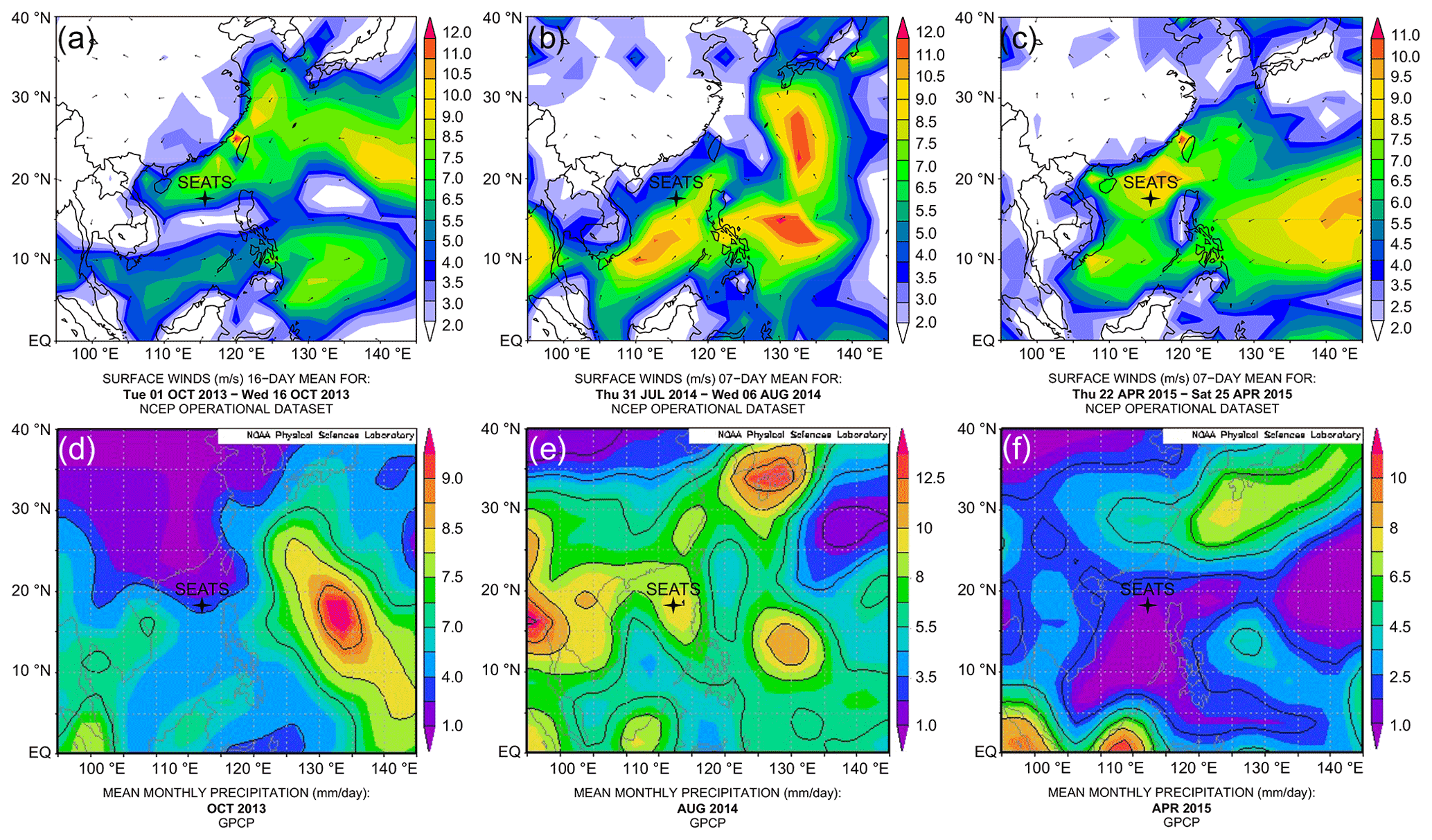
Figure 2Upper panels – surface vector wind maps indicating the monsoon seasons: (a) inter-monsoon period in October 2013; (b) southwest summer monsoon in August 2014; (c) northeast winter monsoon in April 2015. Lower panels – mean monthly precipitation: (d) in October 2013; (e) in August 2014 and (f) in April 2015. Maps of vector wind distributions were obtained from the NOAA – Atmospheric Variables Plotting Page using the NCEP daily analysis data (https://www.esrl.noaa.gov/psd/data/histdata/, last access: April 2020). Maps of precipitation were obtained from NOAA's GPCP Version 2.3 Combined Precipitation Data Set (https://psl.noaa.gov/data/gridded/data.gpcp.html, last access: April 2020).
The chlorophyll fluorescence was generally low and restricted to the thermocline in the upper 50–100 m (Fig. 3), as expected for the oligotrophic northern SCS (see Sect. 1), with the absolute magnitude of the subsurface maximum peak varying between seasons. Interestingly, Chl a was highest with 0.60 mg m−3 in October 2013 (Fig. 3a). In August 2014 the concentration remained at 0.20–0.30 mg m−3 without pronounced variations or diurnal trends (Fig. 3b). In April 2015, we observed a minor increase in the subsurface chlorophyll maximum (but mostly restricted to the dawn hours) of up to 0.50 mg m−3, which gradually declined throughout the day and was lowest at night with approximately 0.20 mg m−3 (Fig. 3c).

Figure 3Fluorescence (mg m−3) time series from SEATS on (a) 16 October 2013, (b) 5–6 August 2014 and (c) 24–25 April 2015. (d) Depth profiles of dissolved O2 saturation (%) during the different sampling days, calibrated to manual dissolved O2 measurements. Data visualization was done using Ocean Data View (https://odv.awi.de/, Schlitzer, 2020).
The dissolved O2 saturation in the upper 400 m on the different sampling days is shown in Fig. 3d. In October 2013, the mixed layer was saturated between 100 % and 102 %, and below in the thermocline the O2 saturation decreased. In August 2014, the O2 was saturated throughout the mixed layer (100 %) on the first collection day and was between 97 %–98 % on the second day. In April 2015, the mixed-layer O2 saturation hovered between 97 %–98 % on the first day and 102 %–103 % on the second day. Below the limit of the mixed layer, O2 saturation increased by a few percent on both days in August 2014 as well as on 24 April 2015. A more prominent supersaturated O2 peak reaching 110 % below the mixed layer was observed on 25 April 2015.
Based on our sampling months and the observed physical parameters, the profile from October 2013 appears to reflect the transition from summer to winter conditions. The lack of basin-wide prevailing monsoon forcing is also evident from surface wind maps (Fig. 2a), indicating that this collection date might largely represent an inter-monsoon period. The shallow mixed layer in August 2014 and southwest wind direction point towards typical summer monsoon conditions (Fig. 2b). Conversely, the mixed-layer characteristics in April 2015 are suggestive of spring conditions, although the surface wind maps still indicate the presence of the northeast winter monsoon in the area (Fig. 2c). We therefore conclude that the April 2015 collection days likely reflect late northeast (winter) monsoon season during spring.
3.2 Dissolved O2 composition: 17Δ and Δ()
The triple isotope composition of dissolved O2 profiles from SEATS is shown in Fig. 4. We observed broad variations in both the 17Δ and the Δ() between the different months as well as the days when the samples were collected, overall ranging between 22 and 229 per meg and −72 % to 2.2 %, respectively. Overall, the upper-ocean 17Δ profiles outlined a common trend, with lower 17Δ in the mixed layer, a peak in the values below and a gradual decrease towards 200 m depth. However, the average mixed-layer values (Table 1) and the depth of the 17Δ maximum peak, as well as its magnitude, varied considerably between months and collection days. Highest mixed-layer 17Δ values averaging 90±28 per meg were observed in October 2013. On 5 and 6 August 2014 and 24 April 2015 the O2 compositions were comparable, yielding mean mixed-layer 17Δ values of 59±9, 54±18 and 52±11 per meg and Δ() values of %, % and %, respectively. Lowest mixed-layer 17Δ values of 26±5 per meg with positive Δ() of 1.8±0.3 % were observed on 25 April 2015.
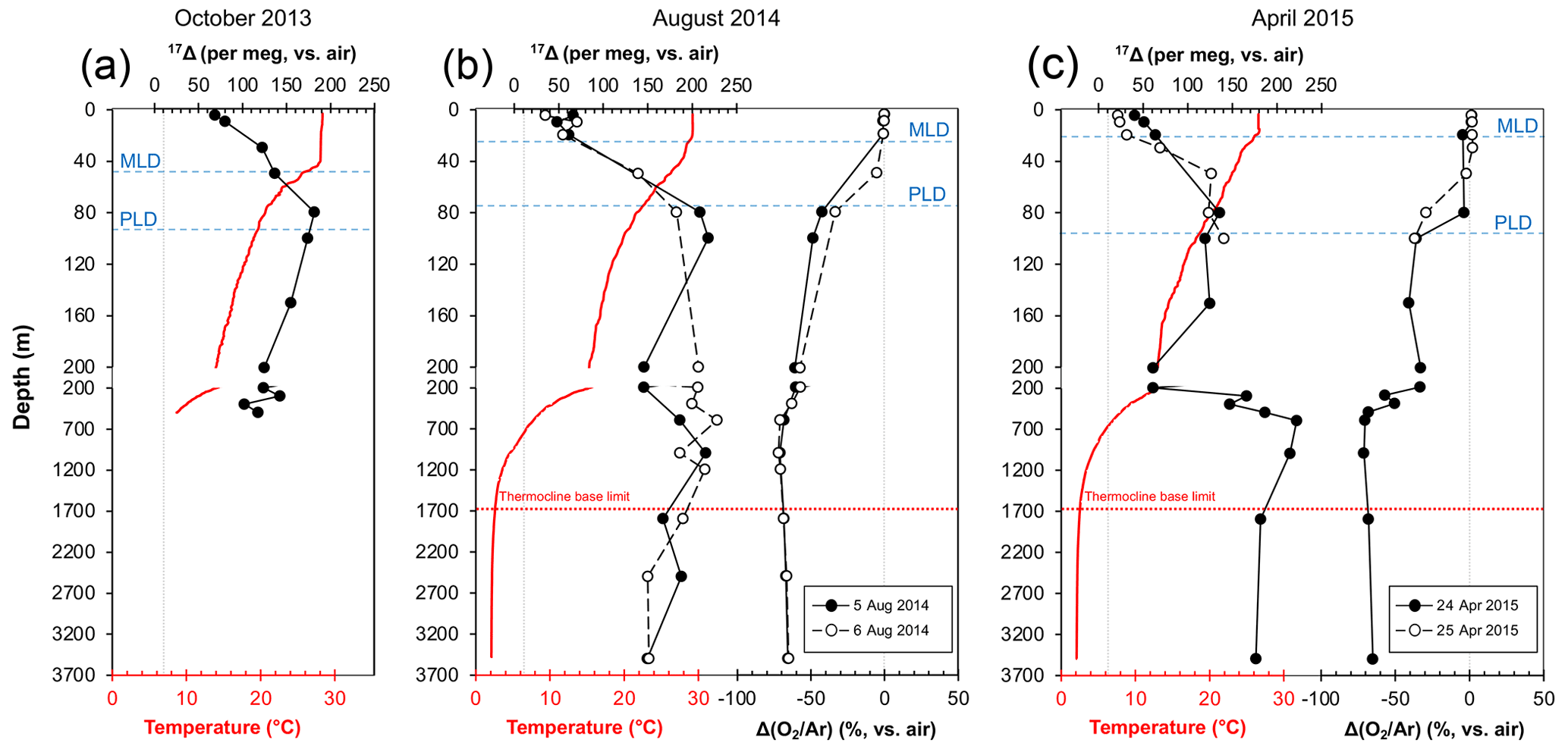
Figure 4Depth profiles of temperature (red lines) and 17Δ and Δ() profiles (solid or dashed black lines) from SEATS from (a) 16 October 2013 (inter-monsoon season), (b) 5–6 August 2014 (summer southwest monsoon) and (c) 24–25 April 2015 (winter northeast monsoon). Vertical dashed grey lines indicate the equilibrium 17Δ and Δ() values with atmosphere. MLD – mixed-layer depth, PLD – photic layer depth.
Largest variations in 17Δ and Δ() were observed within the thermocline. In October 2013, the 17Δ gradually increased with depth to a maximum of 182 per meg at 80 m and then decreased (Fig. 4a). On the 5 August 2014, the highest 17Δ values reached 218 per meg at 100 m (Fig. 4b). The depth trend on the 6 August fairly resembled the one from the 5 August, but the 17Δ values between the 2 sampling days varied up to 61 per meg at 150 m. In April 2015, the 17Δ variations were comparatively subtle, without a prominent sharp peak, ranging between 140 and 125 per meg in the upper 50 to 150 m. A deep peak in 17Δ was observed at 600 m of 223 per meg (Fig. 4c).
4.1 Seasonal trends in photosynthetic vs. atmospheric O2 input in the upper water column
The combined approach of 17Δ and Δ() composition of dissolved O2 has been shown to be a valuable tracer for distinguishing biologically mediated O2 from that supplied by atmospheric air input to the euphotic zone (Luz et al., 1999; Luz and Barkan, 2000). This is because atmospheric O2 has a unique isotopic signature generated by stratospheric photochemical reactions involving O3, O2 and CO2 which fractionate its isotopes in a mass-independent way (see Lämmerzahl et al., 2002), while photosynthesis fractionates O2 isotopes in a mass-dependant way. By definition, the atmospheric 17Δatm=0, although the air–water equilibrium 17Δeq deviates slightly from the atmospheric value ( per meg; see Sect. 2.1; Jurikova et al., 2016) due to fractionation at equilibrium where the δ17O and δ18O slopes (λ) during invasion and evasion follow a slope different to that of respiration. Marine photosynthesis increases the 17Δ of dissolved O2 up to its maximum value of 250 per meg (the 17Δ of seawater), which indicates that the dissolved O2 is completely of photosynthetic origin, while gas exchange with atmosphere drives the 17Δ back towards its equilibrium value. Respiration consumes O2 but does not affect the relative proportion of δ17O and δ18O and hence the 17Δ. Respiration may be traced by Δ() since O2 and Ar are similarly affected by physical processes, but Ar does not have any biological sources and sinks. The coupling between 17Δ and Δ() thus serves as a powerful tool to monitor the photosynthetic vs. atmospheric influences on dissolved O2.
The Δ() values for the October 2013 profile are unfortunately not available, and we are limited to discussing the changes in dissolved O2 content in the context of the 17Δ data only. In comparison to the observations from August 2014 and April 2015, interestingly, during this month we observed considerably elevated 17Δ in the mixed layer (90±28 per meg), implying the presence of biological O2 (Table 1). High 17Δ values, such as the 122 per meg measured at 30 m depth, seem particularly unusual, as any instantaneous increase in photosynthetic 17Δ signal in the mixed layer is expected to be limited due to continuous exchange with atmospheric O2 and thus averaged against the background signal. It is also unlikely that these samples could have been affected by contamination, as any leak during the sampling or preparation would result in a decreased 17Δ value due to influence from atmospheric O2. A likely explanation for the observed high 17Δ would be the rather short O2 production time (<1 d) against the relatively long residence time of O2 in the mixed layer (12 d; see Sect. 2.2), suggesting a sustained accumulation of biologically produced O2. The timing of the high 17Δ values in the mixed layer (Fig. 4a) also coincided with the overall highest observed fluorescence in this study (Fig. 3a). The Chl a maximum was situated below the mixed layer in the thermocline where we also recorded a 17Δ peak. The elevated mixed-layer 17Δ values, therefore, could also reflect a transient increase in biological O2 due to upward flux of photosynthetically produced dissolved O2 from the Chl a maximum horizon. In such a case the 17Δ and the primary production would also integrate O2 from below the mixed layer, and this may complicate the application of the steady-state model. Assuming that these values really reflect the integrated O2 production, it may suggest rather high photosynthetic activity for an inter-monsoon period, probably enhanced by the onset of cooler temperatures after the summer.
The average mixed-layer 17Δ and Δ() values from 5 and 6 August 2014 as well as from 24 April 2015 were, within the variations, indistinguishable from each other (about 55±13 per meg and %; Table 1). The observed 17Δ values reflect the presence of photosynthetic O2, which based on the Δ() values was in near-equilibrium concentrations to potentially slightly undersaturated (especially towards the bottom of the mixed layer if individual measurements are considered). Previous studies have largely disregarded negative mixed-layer Δ() values and attributed them to vertical mixing (Reuer et al., 2007; Stanley et al., 2010). During our sampling period, we did not observe significant upwelling of water (internal wave) that could be indicative of diapycnal mixing and contribution from deeper water to the mixed layer, although data spanning the entire residence time of O2 in the mixed layer would be needed for a more conclusive statement. Recently, Qin et al. (2021) reported Δ() from the northern slope of the SCS collected by continuous measurement of gases in the surface waters (5 m) during approximately 2 weeks in October 2014 and June 2015. While most of their values yielded positive Δ(), the authors also reported negative values which they linked to upwelling caused by a localized cold eddy. Hence, it can be expected that vertical mixing would result in negative Δ() values at 5 m in the SCS which, however, was not observed in our data (our Δ() values at 5 m ranged between 0 % to 1.6 %). Although some degree of exchange across the mixed-layer boundary cannot be excluded, we postulate that, overall, our data reflect a minimal photosynthetic activity characteristic of the summer months at SEATS. This may be attributed to the strong seasonal thermal stratification and nutrient depletion (Wong et al., 2017b), as supported by the measured low fluorescence in August 2014 (Fig. 3b), in agreement with past observations (Liu et al., 2002).
Distinct 17Δ and Δ() values were observed on 25 April 2015 (∼26 per meg and ∼ 1.8 %; Table 1). Although the average mixed-layer signal from 24 April 2015 (52±11 per meg and %) is similar to the values from August 2014, if the deepest mixed-layer sample from 20 m depth were removed from the calculation (despite still being situated within the mixed layer), then the newly obtained mixed-layer Δ() for 24 April 2015 would agree well with the values from 25 April 2015 (1.5±0.2 %; with the 17Δ remaining unaffected 46±7 per meg). This points towards variable conditions near the mixed-layer boundary, potentially influenced by O2 contribution from below waters where the Δ() was negative. The lower, closer to equilibrium, 17Δ values on the second day of sampling indicate increased air–sea gas exchange rates, which drive oxygen production as evidenced by the elevated Δ() in the mixed layer (Fig. 4c). This is further supported by the intensified fluorescence (Fig. 3c) and supersaturated dissolved oxygen waters (Fig. 3d) below the mixed layer. The distribution and concentration of the deep chlorophyll maximum corresponds to characteristic monsoon-forced trends (Liu et al., 2002) and demonstrates the vitality of the thermocline-dwelling phytoplankton and the important role of NEM winds on determining the metabolic balance of the system. The overall lower 17Δ and Δ() values in the upper water column observed in April 2015 when compared to August 2014 (Fig. 4) may illustrate the extent of wind-induced vertical mixing, which could be sufficient to reach the upper limit of the nutricline (e.g. Ning et al., 2004; Tseng et al., 2005) and supply nutrients to the phytoplankton communities. Similar Δ() values were also reported by Qin et al. (2021) for the slope region of the SCS and are typically attributed to nutrients, especially nitrogen, becoming available to phytoplankton. Alternatively, between February and April monsoon winds tend to carry minerals and iron-rich dust particles from the deserts in Central Asia to the northern SCS and SEATS (Lin et al., 2007; Duce et al., 1991; Fung et al., 2000), which could fuel the enhanced biological production. These profiles thus serve as a good example of the local ecosystem interactions and underscore the close dependence of the phytoplankton communities on the NEM forcing.
4.2 Primary production rates in South China Sea
Primary production, the synthesis of organic compounds from carbon-containing species, is of critical importance to biogeochemical cycling of carbon and oxygen that sustains the marine ecosystem. In a steady-state system, we may distinguish gross production (GP) and net production (NP), where the former represents the total C fixed by primary producers and the latter the C available to the heterotrophic community. The NP thus amounts to the difference between the GP and community respiration. NP is positive when GP exceeds respiration, and the ecosystem exports or stores organic C, while negative values result when respiration exceeds GP, and the ecosystem respires more organic C than it was able to produce. These terms are of fundamental interest to ocean studies. However, their quantification is not straightforward, and thus far, only limited information is available globally and especially from SEATS and the SCS.
Our production rates are summarized in Table 1, derived from δ17O and δ18O values of dissolved oxygen using a steady-state mixed-layer oxygen budget model that allows for determining integrated productivity in the mixed layer over the residence time of O2 (as detailed in Sect. 2.2). We note that these estimates, however, do not account for complex physical processes (vertical mixing, lateral advection) and non-steady-state effects on the mass balance. Furthermore, as discussed in Sect. 2.2, the choice of parametrization method and approach for calculating gas exchange rates introduces uncertainties and merits a careful consideration. The definition of the mixed-layer depth is also highly relevant, although as shown both the temperature-based and dissolved-O2-based definition resulted in similar depths in this study. We found that largest uncertainties on the derived production rates (especially on the 16 October 2013 and on the 6 August 2014; Table 1) resulted from variations in δ17O, δ18O and Δ() between samples collected from a vertical profile through the mixed layer. These variations are reported as the standard deviation of the mean composition of dissolved O2 in the mixed layer, and they are considered in the calculation of our NP and GP rates.
We found comparable production rates on the two consecutive sampling days in August 2014, with mean GP ∼ 1500 mg C m−2 d−1, and low NP rates averaging −13 mg C m−2 d−1. Although these rates appear to indicate that the system metabolism was net heterotrophic, within the uncertainties (based on the Δ(), δ17O and δ18O variations in the mixed layer) it was in net balance. Similar values and overall net (or close to net) balance likely prevails in the SCS during the SWM season, as with the exception of sporadic typhoon events, the environmental conditions can be expected to remain rather stable and the water column strongly stratified. The production was also within the errors comparable on 24 April 2015, yielding GP of ∼ 2000 mg C m−2 and NP of ∼ −40 mg C m−2 d−1. On the second sampling day, 25 April, the GP was considerably lower (∼ 600 mg C m−2 d−1), and the NP was higher (∼ 140 mg C m−2 d−1). This points towards a more dynamic system, likely influenced by the NEM conditions. It appears that the NEM forcing could shift the metabolism of the system from being close to net balance to net autotrophy, due to cooler temperatures and wind-induced mixing of the water column, providing nutrients from the subsurface waters into the mixed layer. Potentially, minor contribution to the signal could also come through the input of photosynthetically produced O2 from below the mixed layer. Highest GP estimates of 6600 mg C m−2 d−1 were obtained in October 2013, which is rather surprising since during inter-monsoon periods phytoplankton production is expected to be limited. The origin of the high GP rates in October 2013 appears to be related to the deeper mixed layer on this sampling day. Elevated 17Δ values (122 per meg) were measured at 30 m, with some contribution to the signal potentially coming from the photic layer below. These estimates should, therefore, be treated with caution as diapycnal mixing across the base of the mixed layer, and/or heterogenous distribution of phytoplankton in the water column and potential in situ production at depth cannot be ruled out, in which case the steady state no longer applies.
It is to be stressed that our estimates represent the mixed-layer production rates rather than total water column rates. During our sampling campaigns at SEATS, the euphotic zone was persistently deeper (∼ 30–70 m deeper) than the mixed layer (Table 1, Fig. 4). This may lead to underestimation of the true mixed-layer NP values due to mixing or entrainment of low-O2 waters into the mixed layer and conversely overestimation of the true mixed-layer GP values due to mixing or entrainment of high-17Δ waters into the mixed layer, since the share of the production that takes place within the euphotic zone below the mixed layer cannot be accounted for by the present model. Nonetheless, it is likely that if respiration exceeds gross production in the mixed layer (and hence the NP is negative), the overall NP in the euphotic zone will also be negative, since deeper regions tend to have higher respiration rates. Thus, production estimates from paired 17Δ and Δ() profiles are still useful for indicating trends in ecosystem metabolism even in instances when the depths of the mixed and euphotic layers differ. Our findings indicate that over the year respiration might be close to the GP, with phenomena such as the NEM forcing playing an important role in fuelling productivity. Hence, production during winters with cooler temperatures and windy days may play a decisive role in determining the amount of organic C fixed. For instance, an oligotrophic system that is net heterotrophic most of the time could maintain overall net autotrophy with episodic production which occurs 10 % of the time and is 3 times the background rate (Karl et al., 2003). Weakening of the East Asian Monsoon by anthropogenically induced global warming (e.g. Hsu and Chen, 2002; Xu et al., 2006) is, however, likely to limit vertical transport and nutrient supply to the phytoplankton. It is to be seen to what extent this will affect the primary production and overall C balance at SEATS and in the SCS.
Previous primary production estimates from the SCS based on 14C observations and modelling fall within the range of approximately 120–170 g C m−2 yr−1 (Ning et al., 2004; Chen, 2005; Liu et al., 2002). Ning et al. (2004) studied seasonal patterns in phytoplankton and productivity, and based on 14C bottle incubation experiments, they estimated the summer and winter daily production within the euphotic zone to be 390±342 and 546±409 mg C m−2 d−1, respectively. Although the comparison between incubation-based 14C productivity estimates and those derived from triple oxygen isotopes is not straightforward due to the different natures of the methods and temporal and spatial scales over which they integrate, it is important to attempt to place the different estimates in context of each other. To convert 14C production estimates from bottle incubations to GP, we used a scaling factor of 1.74 to correct for dark respiration and excretion of DO14C (dissolved organic carbon; Hendricks et al., 2004). This gives mean summer-to-winter GP rates of approximately 680–950 mg C m−2 d−1 for the values reported by Ning et al. (2004). Omitting our high GP rates from October 2013, which are likely biased by mixed-layer entrainment, this is lower than our mean rates of about 1410±590 mg C m−2 d−1. Similarly, previous attempts to compare the 14C incubation-based and triple oxygen isotope-based estimates have generally found that the latter estimates tend to overestimate the primary production by a factor of about 1–3 (Juranek and Quay, 2005; Quay et al., 2010; Juranek and Quay, 2013; Jurikova et al., 2016). Whether this is due to a high bias from the triple oxygen approach or a low bias from the bottle incubation method remains a matter of on-going debate, which only further measurements of marine productivity using both incubation-based and incubation-independent methods and comparison studies can resolve. We postulate that some of the high bias we found could be due to vertical mixing with deeper waters (which leads to higher 17Δ). To a larger extent, the observed differences probably result from the low bias of the bottle incubation approach due to containment effects and/or missed infrequent episodes or patches of high productivity (Quay et al., 2010; Juranek and Quay, 2013), which are known to occur in the SCS. Much of our understanding and discussion of productivity in the SCS, however, remains limited by the availability of data, which at present likely only offers a snapshot of the full picture. Crucially, further measurements of primary productivity at an increased spatial and temporal resolution will provide a more comprehensive picture of production at SEATS and within the wider SCS, reduce the uncertainties involved and inform the discussion of methodological biases.
4.3 Comparison to other tropical time series
Initially launched in 1998, and becoming part of the Joint Global Ocean Flux Study 1 year later (JGOFS; Shiah et al., 1999), the SEATS station has often been compared with the time series off Hawaii (the Hawaii Ocean Time-series, HOT), which together with the time series off Bermuda (the Bermuda Atlantic Time-series Study, BATS) were two key components of the former JGOFS programme. In contrast to the typical features of tropical waters, characterized by minimal seasonal variations, and comparing to the low-latitude HOT station (Karl and Lukas, 1996), the SEATS station located at an even lower latitude is characterized by a distinct phytoplankton biomass and primary production pattern (Tseng et al., 2005; Wong et al., 2007a). This distinct pattern is largely governed by the East Asian Monsoon, which brings seasonal changes that affect the oceanography and biogeochemistry of the SCS (Chao et al., 1996a; Liu et al., 2002).
Our seasonal depth profiles from SEATS share some similarities with the tropical oligotrophic HOT station (Juranek and Quay, 2005), albeit with different 17Δ magnitudes. Notably, the 17Δ depth distribution pattern at SEATS was comparable to that at HOT, with a broad summer 17Δ peak (above 200 per meg at 80 and 100 m depth) from August 2014 comparable to that at HOT during the same month (with values above 140 per meg at 120 and 150 m depth), as well as a high peak in October 2013 (above 180 per meg at 80 m) rather similar to that at HOT during October (above 140 per meg at 100 m). In February, the 17Δ values were overall much lower at HOT, reaching the highest values in the deep (above 90 per meg between 150 and 200 m). Possibly, such trends could also be expected for SEATS; in fact our data from April 2015 appear to bear a close resemblance to this pattern, although a comparison of the same months would be preferable. Our maximum 17Δ values within the euphotic zone at SEATS (218 per meg at 100 m observed on 5 August 2014, Fig. 4b) are, however, to our knowledge much higher than any previously documented upper-ocean values at HOT or elsewhere, which typically do not exceed ∼ 160 per meg.
Obviating the estimates from October 2013, our GP and NP rates are comparable to those from HOT derived using the same approach, where seasonal variation in GP and NP were in the range of 800–1470 mg C m−2 d−1 and −120 and 180 mg C m−2 d−1 (Juranek and Quay, 2005). Generally, we would, however, expect higher rates at SEATS, where both seasonal monsoon forcing and/or episodic typhoon events induce sufficient vertical mixing to bring nutrients to the mixed layer and stimulate primary production. Assuming that our rates present an underestimation of the productivity due to the relatively very shallow mixed layer, these differences could reconcile. Our observed variations in (∼ −0.01 in August 2014 and between −0.02 and 0.23 in April 2015) also compare well with the seasonal trends reported from HOT (between −0.13 and 0.13 during summer and winter; Juranek and Quay, 2005) with tendency towards heterotrophy in the summer and autotrophy during winter months. Very low ratios were also observed from other low-latitude regions such as the equatorial Pacific (Hendricks et al., 2005; Stanley et al., 2010). This supports the general parallels in ecosystem metabolism in the oligotrophic regions, but also given the broader variations in ratios at SEATS, it emphasizes the importance of the monsoon forcing on introducing dynamics to this system.
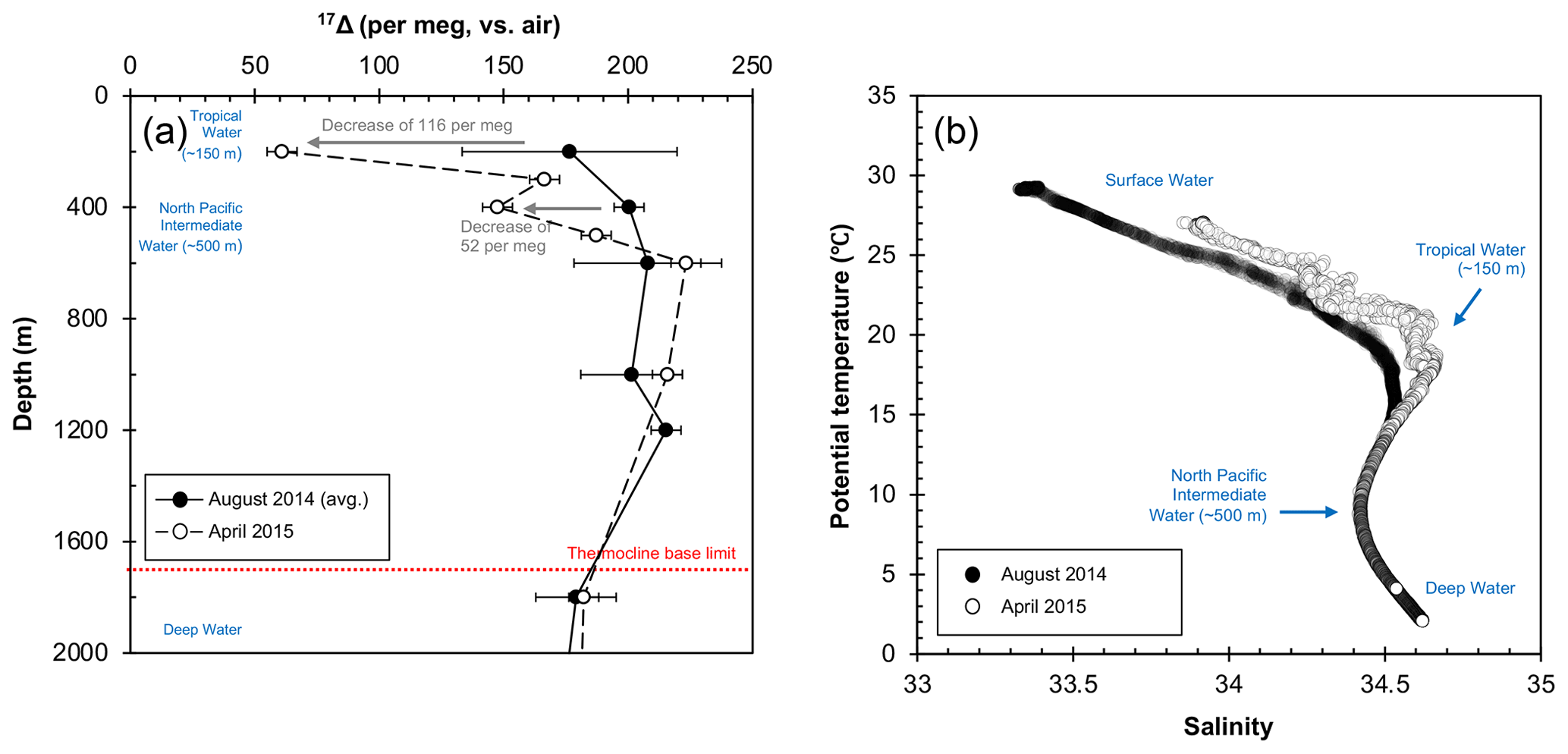
Figure 5Deep water composition at SEATS from August 2014 to April 2015; (a) 17Δ of dissolved O2. The 17Δ values from August 2014 are shown as mean of the 2 sampling days (5 and 6 August). Error bars indicate the standard deviation between the 2 collection days (1σ) where available or the analytical uncertainty (6 per meg; 1σ). (b) Relationship between potential temperature and salinity. Salinity peak of ∼ 34.6 (and ∼ 20 ∘C) corresponds to the Tropical Water situated around 150 m, while the minimum of ∼ 34.4 indicates the North Pacific Intermediate Water at around 500 m. The Deep Water below the thermocline base (∼ 1700 m) is characterized by low temperatures of ∼ 2 ∘C and high salinities around ∼ 34.6.
4.4 New insights into the 17Δ in deep water
The 17Δ has been traditionally applied for evaluating primary production in the upper ocean, and thus far, only little is known on the 17Δ composition of the deep ocean. Due to the conservative behaviour of O2 in a parcel of deep water where it may no longer be influenced by air–sea gas exchange or photosynthesis, the 17Δ could also present a valuable tracer for deep water mixing processes since any variations in 17Δ should principally result from mixing of waters with different 17Δ values. While respiration alone does not affect the tracer, the 17Δ may, however, behave non-conservatively and be altered by the combined effects of respiration and mixing. As shown by Nicholson et al. (2014), if two hypothetical parcels of water with very different δ17O and δ18O values (but same 17Δ values) mix (one with the starting composition of surface water and one that underwent a Rayleigh fractionation until 5 % of oxygen remained), the resulting 17Δ values can become negative. Subsurface (∼ 100–300 m) measurements in the equatorial Pacific indeed reported few negative values (Hendricks et al., 2005). Measurements from deeper profiles (700 m) were carried out in the Gulf of Elat and showed that the 17Δ values below the thermocline varied considerably with seasons, a likely result of vertical as well as horizontal mixing (Wurgaft et al., 2013). In order to evaluate the behaviour of 17Δ in the deep water of the SCS and its potential utility as a mixing tracer in an oceanographically very distinct system, we measured the 17Δ composition of deep O2 profiles (down to 3500 m depth) from SEATS.
An overview of the oceanography of SCS is available in Wong et al. (2007a). The subsurface water masses in the SCS consist of three main water masses: (1) the Tropical Water situated at around 150 m, originating from near the international dateline at 20–30∘ N in the North Pacific (Suga et al., 2003); (2) the North Pacific Intermediate Water centred around 500 m with a source in the subpolar regions in the North Pacific (You, 2003); and (3) the Deep Water below 2200 m. The Deep Water in the SCS basin is formed by Pacific water masses, which in the western Philippine Sea overflow the sill that separates it from the SCS. The characteristics of the deep water in the SCS are rather uniform and similar to those in the western Philippine Sea. They are maintained by a mass balance between the inflowing deep water from the Philippine Sea, upwelling and mixing with the shallower North Pacific Intermediate Water, and outflow at an intermediate depth through Luzon Strait (Gong et al., 1992; Chao et al., 1996b; Hu et al., 2000).
Our data showed overall elevated 17Δ values (>140 per meg) below 200 m depth for both August 2014 and April 2015 profiles. Largest variations were found at 200 m with a decrease of 116 per meg from August 2014 to April 2015 (Fig. 5a), coinciding with changes in the temperature–salinity characteristics of the Tropical Water mass (Fig. 5b). The synergic decrease in 17Δ and increase in temperature–salinity at this depth illustrate the increased winter inflow of water to the SCS from Kuroshio through the Luzon Strait or possibly also partially from the East China Sea through the Taiwan Strait (Fig. 1). This highlights the importance of NEM winds in driving the seasonal circulation inducing vertical mixing, which extends down to 400 m and leads to a full exchange of water masses during a winter (Fig. 5a). Historic records also support intrusions of North Pacific water masses to the SCS all-year round with greatest strength in winter (Qu et al., 2000). Below, the deeper water remained relatively homogenous, and it did not appear to be influenced by seasonal changes, marking the limit of the extent of monsoon-driven circulation influence on the mixing. Surprisingly, variations in 17Δ (around ∼ 20 per meg) were found beneath the thermocline base; however, considering the low O2 content at these depths, even a very minor change in O2 concentration may result in a large effect on the 17Δ signal. Although further observations from the SCS are needed for a more comprehensive picture, our first results advocate for the 17Δ as a valuable tracer of mixing processes, which brings new insights into some of the key aspects of our understanding of the circulation in the SCS.
In summary, in this study we provided the first insights into the 17Δ composition of dissolved O2 at the SEATS station and within the South China Sea (SCS). We used the combined 17Δ and Δ() approach to monitor the seasonal changes in atmospheric vs. photosynthetic O2 input to the upper part of the ocean and to calculate the integrated mixed-layer GP and NP rates. Our results showed that the net biological production at SEATS was negligible during most sampling days and close to net zero but increased when the system was more dynamic during a spring influenced by the northeast monsoon forcing. Mixed-layer variations and potential O2 contribution from below the mixed layer, however, contribute uncertainties to these estimates and should be taken into consideration in further work applying this tracer, in particular within the SCS. Furthermore, we found the 17Δ of the deep water to be a promising tracer for physical mixing process (in addition to biological processes). This permitted us to evaluate the extent of the basin-wide monsoon-driven circulation in the water column and at depth, as well as to revisit the deep mixing processes. Although further work is required before the deep 17Δ may be confidently applied as a tracer of water mass mixing, our study showed that it could bring new perspectives on the renewal rate of the deep water, at least within the SCS. Thus, further deep 17Δ measurements within the region but also globally would be desirable. Similarly, further 17Δ and Δ() measurements within the SCS at an increased spatio-temporal resolution would be beneficial for gaining a more comprehensive picture of primary productivity dynamics at SEATS and its link and responses to the East Asian Monsoon as well as other episodic or interannual phenomena.
The data used in this study are available in the Supplement including geochemical data (Tables S1 and S2), CTD data (Table S3) and wind speed data (Table S4).
The supplement related to this article is available online at: https://doi.org/10.5194/bg-19-2043-2022-supplement.
HJ and MCL designed the study and performed the analyses. OA and FKS contributed analytics tools and data. HJ prepared the article with contributions from all co-authors.
The contact author has declared that neither they nor their co-authors have any competing interests.
Publisher’s note: Copernicus Publications remains neutral with regard to jurisdictional claims in published maps and institutional affiliations.
We thank Wei-Kang Ho for help with sample collection, analysis, and instrumental support; Chao-Chen Lai, Hsiang-Yi Kuo, Kuo-Yuan Lee, and Jen-Hua Tai for assistance during sampling and providing us with shipboard data; and Hsin-Chien Liang for providing us with satellite data (from the Research Center for Environmental Changes, Academia Sinica). Support from Taiwan's R/V Ocean Researcher-1 and the crew members is gratefully acknowledged. We are thankful to the referees for their thoughtful comments and constructive reviews, which helped us improve the quality of the article.
This research has been supported by the Ministry of Science and Technology, Taiwan (grant no. 108-2111-M-001-011-MY3) and the Academia Sinica (grant no. AS-IA-109-M03).
This paper was edited by Carol Robinson and reviewed by Karel Castro-Morales and two anonymous referees.
Barkan, E. and Luz, B.: High-precision measurements of and of O2 and ratio in air, Rapid Commun. Mass Sp., 17, 2809–2814, https://doi.org/10.1002/rcm.1267, 2003.
Benson, B. B. and Krause Jr., D. K.: The concentration and isotopic fractionation of oxygen dissolved in freshwater and seawater in equilibrium with the atmosphere, Limnol. Oceanogr., 29, 620–632, https://doi.org/10.4319/lo.1984.29.3.0620, 1984.
Cai, W.-J. and Dai, M.: Comment on “Enhanced open ocean storage of CO2 from shelf sea pumping”, Science, 306, 1477, https://doi.org/10.1126/science.1102132, 2004.
Carr, M.-E., Friedrichs, M. A. M., Schmeltz, M., Aita, M. N., Antoine, D., Arrigo, K. R., Asanuma, I., Aumont, O., Barber, R., Behrenfeld, M., Bidigare, R., Buitenhuis, E. T., Campbell, J., Ciotti, A., Dierssen, H., Dowell, M., Dunne, J., Esaias, W., Gentili, B., Gregg, W., Groom, S., Hoepffner, N., Ishizaka, J., Kameda, T., Le Quéré, C., Lohrenz, S., Marra, J., Mélin, F., Moore, K., Morel, A., Reddy, T. E., Ryan, J., Scardi, M., Smyth, T., Turpie, K., Tilstone, G., Waters, K., and Yamanaka, Y.: A comparison of global estimates of marine primary production from ocean color, Deep-Sea Res. Pt. II, 53, 741–770, https://doi.org/10.1016/j.dsr2.2006.01.028, 2006.
Castro-Morales, K. and Kaiser, J.: Using dissolved oxygen concentrations to determine mixed layer depths in the Bellingshausen Sea, Ocean Sci., 8, 1–10, https://doi.org/10.5194/os-8-1-2012, 2012.
Castro-Morales, K., Cassar, N., Shoosmith, D. R., and Kaiser, J.: Biological production in the Bellingshausen Sea from oxygen-to-argon ratios and oxygen triple isotopes, Biogeosciences, 10, 2273–2291, https://doi.org/10.5194/bg-10-2273-2013, 2013.
Chao, S.-Y., Shaw, P.-T., and Wu, S. S.: El Niño modulation of the South China Sea circulation, Prog. Oceanogr., 38, 51–93, https://doi.org/10.1016/S0079-6611(96)00010-9, 1996a.
Chao, S.-Y., Shaw, P.-T., and Wu, S. S.: Deep water ventilation in the South China Sea, Deep-Sea Res. Pt. I, 43, 445–466, https://doi.org/10.1016/0967-0637(96)00025-8, 1996b.
Chen, C.-C., Shiah, F.-K., Chung, S.-W., and Liu, K.-K.: Winter phytoplankton blooms in the shallow mixed layer of the South China Sea enahnced by upwelling. J. Marine Syst., 59, 97–110, https://doi.org/10.1016/j.jmarsys.2005.09.002, 2006.
Chen, C.-T. A., Liu, K.-K., and Macdonald R.: Continental margin exchanges, in: Ocean Biogeochemistry: The Role of the Ocean Carbon Cycle in Global Change, edited by: Fasham, M. J. R., Springer, New York, 53–98, https://doi.org/10.1007/978-3-642-55844-3_4, 2003.
Chen, Y. L.: Spatial and seasonal variations of nitrate-based new production and primary production in the South China Sea, Deep-Sea Res. Pt. I, 52, 319–340, https://doi.org/10.1016/j.dsr.2004.11.001, 2005.
Craig, H. and Hayward, T.: Oxygen Supersaturation in the Ocean: Biological Versus Physical Contributions, Science, 288, 2028–2031, https://doi.org/10.1126/science.288.5473.2028, 1987.
DeGrandpre, M. D., Olbu, G. J., Beatty, C. M., and Hammar, T. R.: Air-CO2 fluxes on the US Middle Atlantic Bight, Deep-Sea Res. Pt. II, 49, 4355–4367, https://doi.org/10.1016/S0967-0645(02)00122-4, 2002.
Duce, R. A., Liss, P. S., Merrill, J. T., Atlas, E. L., Buat-Menard, P., Hicks, B. B., Miller, J. M., Prospero, J. M., Arimoto, R., Church, T. M., Ellis, W., Galloway, J. N., Hansen, L., Jickells, T. D., Knap, A. H., Reinhardt, K. H., Schneider, B., Soudine, A., Tokos, J. J., Tsunogai, S., Wollast, R., and Zhou, M.: The atmospheric input of trace species to the world ocean. Global Biogeochem. Cy., 5, 193–259, https://doi.org/10.1029/91GB01778, 1991.
Emerson S., Quay P. D., Stump C., Wilbur D., and Schudlich R.: Chemical tracers of productivity and respiration in the subtropical Pacific Ocean, J. Geophys. Res.-Oceans, 100, 15873–15887, https://doi.org/10.1029/95JC01333, 1995.
Frankignoulle, M. and Borges, A. V.: European continental shelf as a significant sink for atmospheric carbon dioxide, Global Biogeochem. Cy., 15, 569–576, https://doi.org/10.1029/2000GB001307, 2001.
Fung, I. Y., Meyn, S. K., Tegen, I., Doney, S. C., John, J. G., and Bishop J. K. B.: Iron supply and demand in the upper ocean, Global Biogeochem. Cy., 14, 281–296, https://doi.org/10.1029/1999GB900059, 2000.
Gong, G.-C., Liu, K. K., Liu, C.-T., and Pai, S.-C.: The chemical hydrography of the South China Sea west of Luzon and a comparison with the West Philippine Sea, TAO, 3, 587–602, https://doi.org/10.3319/TAO.1992.3.4.587(O), 1992.
Gong, G.-C., Chen, Y.-L. L., and Liu, K.-K.: Chemical hydrography and chlorophyll a distribution in the East China Sea in summer: implications in nutrient dynamics, Cont. Shelf Res., 16, 1561–1590, https://doi.org/10.1016/0278-4343(96)00005-2, 1996.
Hamme, R. C., Cassar, N., Lance, V. P., Vaillancourt, R. D., Bender, M. L., Strutton, P. G., Moore, T. S., DeGrandpre, M. D., Sabine, C. L., Ho, D. T., and Hargreaves, B. R.: Dissolved and other methods reveal rapid changes in productivity during a Lagrangian experiment in the Southern Ocean, J. Geophys. Res., 117, C00F12, https://doi.org/10.1029/2011JC007046, 2012.
Hendricks, M. B., Bender, M. L., and Barnett, B. A.: Net and gross O2 production in the Southern Ocean from measurements of biological O2 saturation and its triple isotope composition, Deep-Sea Res. Pt. I, 51, 1541–1561, https://doi.org/10.1016/j.dsr.2004.06.006, 2004.
Hendricks, M. B., Bender, M. L., Barnett, B. A., Strutton, P., and Chavez F. P.: Triple oxygen isotope composition of dissolved O2 in the equatorial Pacific: A tracer of mixing, production, and respiration, J. Geophys. Res., 110, C12021, https://doi.org/10.1029/2004JC002735, 2005.
Hu, J., Kawamura, H., Hong, H., and Qi, Y.: A Review on the Currents in the South China Sea: Seasonal Circulation, South China Sea Warm Current and Kuroshio Intrusion, J. Oceanogr., 56, 607–624, https://doi.org/10.1023/A:1011117531252, 2000.
Hsu, H.-H. and Chen, C.-T.: Observed and projected climate change in Taiwan, Meteorol. Atmos. Phys., 79, 87–104, https://doi.org/10.1007/s703-002-8230-x, 2002.
Juranek, L. W. and Quay, P. D.: In vitro and in situ gross primary and net community production in the North Pacific Subtropical Gyre using labelled and natural abundance isotopes of dissolved O2, Global Biogeochem. Cy., 19, GB30009, https://doi.org/10.1029/2004GB002384, 2005.
Juranek, L. W. and Quay, P. D.: Using triple isotopes of dissolved oxygen to evaluate global marine productivity, Annual Rev. Mar. Sci., 5, 503–524, https://doi.org/10.1146/annurev-marine-121211-172430, 2013.
Juranek, L. W., Quay, P. D., Feely, R. A., Lockwood, D., Karl, D. M., and Church, M. J.: Biological production in the NE Pacific and its influence on air-sea CO2 flux: Evidence from dissolved oxygen isotopes and , J. Geophys. Res., 117, C05043, https://doi.org/10.1029/2011JC007450, 2012.
Jurikova, H., Guha, T., Abe, O., Shiah, F.-K., Wang, C.-H., and Liang, M.-C.: Variations in triple isotope composition of dissolved oxygen and primary production in a subtropical reservoir, Biogeosciences, 13, 6683–6698, https://doi.org/10.5194/bg-13-6683-2016, 2016.
Kaiser, J.: Technical note: Consistent calculation of aquatic gross production from oxygen triple isotope measurements, Biogeosciences, 8, 1793–1811, https://doi.org/10.5194/bg-8-1793-2011, 2011.
Kaiser, J., Reuer, M. K., Barnett, B., and Bender, M. L.: Marine productivity estimates from ratio measurements by membrane inlet mass spectrometry, J. Geophys. Res., 32, L19605, https://doi.org/10.1029/2005GL023459, 2005.
Karl, D. M. and Lukas, R.: The Hawaii Ocean Time-series (HOT) program: Background, rationale and field implementation, Deep-Sea Res. Pt. II, 43, 129–156, https://doi.org/10.1016/0967-0645(96)00005-7, 1996.
Karl, D. M., Laws, E. A., Morris, P., Williams, P. J. L. B., and Emerson, S.: Metabolic balance in the open sea, Nature, 462, 32, https://doi.org/10.1038/426032a, 2003.
Lai, C.-C., Wu, C.-R., Chuang, C.-Y., Tai, J.-H., Lee, K.-Y., Kuo, H.-Y., and Shiah, F.-K.: Phytoplankton and Bacterial Responses to Monsoon-Driven Water Masses Mixing in the Kuroshio Off the East Coast of Taiwan, Front. Mar. Sci., 8, 707807, https://doi.org/10.3389/fmars.2021.707807, 2021.
Lämmerzahl, P., Röckmann, T., Brenninkmeijer, C. A. M., Krankowsky, D., and Mauersberger, K.: Oxygen isotope composition of stratospheric carbon dioxide, Geophys. Res. Lett., 29, 1582, https://doi.org/10.1029/2001GL014343, 2002.
Laws, E. A.: Photosynthetic quotients, new production and net community production in the open ocean, Deep-Sea Res. Pt. I, 38, 143–167, https://doi.org/10.1016/0198-0149(91)90059-O, 1991.
Laws, E. A., Landry, M. R., Barber, R. T., Campbell, L., Dickson, M. L., and Marra, J.: Carbon cycling in primary production bottle incubations: inferences from grazing experiments and photosynthetic studies using 14C and 18O in the Arabian Sea, Deep-Sea Res. Pt. II, 47, 1339–1352, https://doi.org/10.1016/S0967-0645(99)00146-0, 2000.
Li, H., Wiesner, M. G., Chen, J., Ling, Z., Zhang, J., and Ran, L.: Long-term variation of mesopelagic biogenic flux in the central South China Sea: Impact of monsoonal seasonality and mesoscale eddy, Deep-Sea Res. Pt. I, 126, 62–72, https://doi.org/10.1016/j.dsr.2017.05.012, 2017.
Liang, M.-C. and Mahata, S.: Oxygen anomaly in near surface carbon dioxide reveals deep stratospheric intrusion, Sci. Rep.-UK, 5, 11352, https://doi.org/10.1038/srep11352, 2015.
Liang, M.-C., Mahata, S., Laskar, A. H., Thiemens, M. H., and Newman, S.: Oxygen isotope anomaly in tropospheric CO2 and implications for CO2 residence time in the atmosphere and gross primary productivity, Sci. Rep.-UK, 7, 13180, https://doi.org/10.1038/s41598-017-12774-w, 2017.
Lin, I.-I., Liu, W. T., Wu, C.-C., Wong, G. T. F., Hu, C., Chen, Z., Liang, W.-D., Yang, Y., and Liu, K.-K.: New evidence for enhanced ocean primary production triggered by tropical cyclone, Geophys. Res. Lett., 30, 1718, https://doi.org/10.1029/2003GL017141, 2003.
Lin, I.-I., Chen, J.-P., Wong, G. T. F., Huang, C.-W., and Lien, C.-C.: Aerosol input to the South China Sea: Results from the MODerate Resolution Imaging Spectro-radiometer, the quick Scatterometer, and the Measurements of Pollution in the Troposphere Sensor, Deep-Sea Res. Pt. II, 54, 1589–1601, https://doi.org/10.1016/j.dsr2.2007.05.013, 2007.
Lin, I.-I., Lien, C.-C., Wu, C.-R., Wong, G. T. F., Huang, C.-W., and Chiang, T.-L.: Enhanced primary production in the oligotrophic South China Sea by eddy injection in spring, Geophys. Res. Lett., 37, L16602, https://doi.org/10.1029/2010GL043872, 2010.
Liu, K.-K., Atkinson, L., Chen, C. T. A., Gao, S., Hall, J., MacDonald, R. W., McManus, L. T., and Quiñones, R.: Exploring continental margin carbon fluxes on a global scale, EOS, 81, 641–644, https://doi.org/10.1029/EO081i052p00641-01, 2000.
Liu, K.-K., Chao, S.-Y., Shaw, P. T., Gong, G.-C., Chen, C.-C., and Tang, T. Y.: Monsoon-forced chlorophyll distribution and primary production in the South China Sea: observations and a numerical study, Deep-Sea Res. Pt. I, 49, 1387–1412, https://doi.org/10.1016/S0967-0637(02)00035-3, 2002.
Lorenzen, C. J.: Chlorophyll b in the eastern North Pacific Ocean, Deep-Sea Res., 28A, 1049–1056, https://doi.org/10.1016/0198-0149(81)90017-0, 1981.
Luz, B. and Barkan, E.: Assessment of Oceanic Productivity with the Triple-Isotope Composition of Dissolved Oxygen, Science, 288, 2028–2031, https://doi.org/10.1126/science.288.5473.2028, 2000.
Luz, B. and Barkan, E.: The isotopic ratios and in molecular oxygen and their significance in biogeochemistry, Geochim. Cosmochim. Ac., 69, 1099–1110, https://doi.org/10.1016/j.gca.2004.09.001, 2005.
Luz, B. and Barkan, E.: Proper estimation of marine gross O2 production with and ratios of dissolved O2, Geophys. Res. Lett., 38, L19606, https://doi.org/10.1029/2011GL049138, 2011.
Luz, B., Barkan, E., Bender, M. L., Thiemens, M. H., and Boering, K. A.: Triple-isotope composition of atmospheric oxygen as a tracer of biosphere productivity, Nature, 400, 547–550, https://doi.org/10.1038/22987, 1999.
Luz, B., Barkan, E., Sagi, Y., and Yacobi, Y. Z.: Evaluation of community respiratory mechanisms with oxygen isotopes: A case study in Lake Kinneret, Limnol. Oceanogr., 47, 33–42, https://doi.org/10.4319/lo.2002.47.1.0033, 2002.
Mahata, S., Bhattacharya, S. K., Wang, C.-H., and Liang, M.-C.: An improved CeO2 method for high-precision measurements of ratios for atmospheric carbon dioxide, Rapid Commun. Mass Spectrom., 26, 1909–1922, https://doi.org/10.1002/rcm.6296, 2012.
Marra, J.: Approaches to the measurement of plankton production, Phytoplankton productivity: carbon assimilation in marine and freshwater ecosystem, edited by: Willams, P. J. le B., Thomas, D. N., and Reynolds, C. S., Cambridge, Blackwells, 78–108, https://doi.org/10.1002/9780470995204.ch4, 2002.
Nicholson, D., Stanley, R. H. R., and Doney, S. C.: The triple oxygen isotope tracer of primary productivity in a dynamic ocean model: Triple oxygen isotopes in a global model, Global Biogeochem. Cy., 28, 538–552, https://doi.org/10.1002/2013GB004704, 2014.
Ning, X., Chai, F., Xue, H., Cai, Y., Liu, C., and Shi, J.: Physical-biological oceanographic coupling influencing phytoplankton and primary production in the South China Sea, J. Geophys. Res., 1009, C10005, https://doi.org/10.1029/2004JC002365, 2004.
Pai, S. C., Gong, G. C., and Liu, K. K.: Determination of dissolved oxygen in seawater by direct spectrophotometry of total iodine, Mar. Chem., 41, 343–351, https://doi.org/10.1016/0304-4203(93)90266-Q, 1993.
Prokopenko, M. G., Pauluis, O. M., Granger, J., and Yeung, L. Y.: Exact evaluation of gross photosynthetic production from the oxygen triple-isotope composition of O2: Implications for the net-to-gross primary production ratios, Geophys. Res. Lett., 38, L14603, https://doi.org/10.1029/2011GL047652, 2011.
Qin, C., Zhang, G., Zheng, W., Han, Y., and Liu, S.: High-resolution distributions of on the northern slope of the South China Sea and estimates of net community production, Ocean Sci., 17, 249–264, https://doi.org/10.5194/os-17-249-2021, 2021.
Qu, T., Mitsudera, H., and Yamagata, T.: Intrusion of the North Pacific waters into the South China Sea, J. Geophys. Res., 105, 6415–6424, https://doi.org/10.1029/1999JC900323, 2000.
Qu, T., Du, Y., Meyers, G., Ishida, A., and Wang, D.: Connecting the tropical Pacific with Indian Ocean through South China Sea, Geophys. Res. Lett., 32, L24609, https://doi.org/10.1029/2005GL024698, 2005.
Quay, P. D., Peacock, C., Björkman, K., and Karl, D. M.: Measuring primary production rates in the ocean: Enigmatic results between incubation and non-incubation methods at Station ALOHA, Global Biogeochem. Cy., 24, GB3014, https://doi.org/10.1029/2009GB003665, 2010.
Regaudie-de-Gioux, A., Lasternas, S., Augustí, S., and Duarte, C. M.: Comparing marine primary production estimates through different methods and development of conversion equations, Frontiers in Marine Science, 1, 19, https://doi.org/10.3389/fmars.2014.00019, 2014.
Rehder, G. and Suess, E.: Methane and pCO2 in the Kuroshio and the South China Sea during maximum summer surface temperatures, Mar. Chem., 75, 89–108, https://doi.org/10.1016/S0304-4203(01)00026-3, 2001.
Reuer, M. K., Barnett, B. A., Bender, M. L., Falkowski, P. G., and Hendricks, M. B.: New estimates of Southern Ocean biological production rates from ratios and the triple isotope composition of O2, Deep-Sea Res. Pt. I, 54, 951–974, https://doi.org/10.1016/j.dsr.2007.02.007, 2007.
Sarma, V. V. S. S., Abe, O., Hashimoto, S., Hinuma, A., and Saino, T.: Seasonal variations in triple oxygen isotopes and gross oxygen production in the Sagami Bay, central Japan, Limnol. Oceanogr., 50, 544–552, https://doi.org/10.4319/lo.2005.50.2.0544, 2005.
Schlitzer, R.: Ocean Data View, https://odv.awi.de/, last access: April 2020.
Seguro, I., Marca, A. D., Painting, S. J., Shutler, J., Suggett, D. J., and Kaiser, J.: High-resolution net and gross biological production during a Celtic Sea spring bloom, Prog. Oceanogr., 177, 101885, https://doi.org/10.1016/j.pocean.2017.12.003, 2019.
Shang, S., Zhang, C., Hong, H., Liu, Q., Wong, G. T. F., Hu, C., and Huang, B.: Hydrographic and biological changes in the Taiwan Strait during the 1997–1998 El Niño winter, Geophys. Res. Lett., 32, L11601, https://doi.org/10.1029/2005GL022578, 2005.
Shiah, F.-K., Liu, K.-K., and Tang, T.-Y.: South East Asian Time-series Station established in South China Sea, US JGOFS Newsletter, 10, 8–9, 1999.
Stanley, R. H. R., Kirkpatrick, J. B., Cassar, N., Barnett, B. A., and Bender, M. L.: Net community production and gross primary production rates in the western equatorial Pacific, Global Biogeochem. Cy., 24, GB4001, https://doi.org/10.1029/2009GB003651, 2010.
Steeman-Nielsen, E.: The use of radioactive carbon (14C) for measuring organic production in the sea, ICES J. Mar. Sci., 18, 117–140, https://doi.org/10.1093/icesjms/18.2.117, 1952.
Strickland, J. D. H. and Parsons, T. R.: A Practical Handbook of Seawater Analysis, Bulletin 167, 2nd Edn., edited by: Stevenson, J. C., Fisheries Research Board of Canada, Ottawa, 1972.
Suga, T., Kato, A., and Hanawa, K.: North Pacific Tropical Water: its climatology and temporal changes associated with the climate regime shift in the 1970s, Prog. Oceanogr., 47, 223–256, https://doi.org/10.1016/S0079-6611(00)00037-9, 2003.
Tai, J.-H., Wong, G. T. F., and Pan, X.: Upper water structure and mixed layer depth in tropical waters: The SEATS station in the northern South China Sea, TAO, 28, 1019–1032, https://doi.org/10.3319/TAO.2017.01.09.01, 2017.
Tai, J.-H., Chou, W.-C., Hung, C.-C., Wu, K.-C., Chen, Y.-H., Chen, T.-Y., Gong, G.-C., Shiah, F.-K., and Chow, C. H.: Short-term variability of biological production and CO2 system around Dongsha Atoll of the northern South China Sea: Impact of topography-flow interation, Front. Mar. Sci., 7, 511, https://doi.org/10.3389/fmars.2020.00511, 2020.
Thomas, H., Bozec, Y., Elkalay, K., and de Baar, H. J. W.: Enhanced Open Ocean Storage of CO2 from Shelf Sea Pumping, Science, 304, 1005–1008, https://doi.org/10.1126/science.1095491, 2004.
Tseng, C.-M., Wong, G. T. F., Lin, I.-I., Wu, C.-R., and Liu, K.-K.: A unique seasonal pattern in phytoplankton biomass in low-latitude waters in the South China Sea, Geophys. Res. Lett., 32, L08608, https://doi.org/10.1029/2004GL022111, 2005.
Tseng, C.-M., Wong, G. T. F., Chou, W.-C., Lee, B.-S., Sheu, D.-D., and Liu, K.-K.: Temporal variations in the carbonate system in the upper layer at the SEATS, Deep-Sea Res. Pt. II, 54, 1448–1468, https://doi.org/10.1016/j.dsr2.2007.05.003, 2007.
Tseng, C.-M., Liu, K.-K., Wang, L.-W., and Gong, G.-C.: Anomalous hydrographic and biological conditions in the northern South China Sea during the 1997–1998 El Niño and comparisons with the equatorial Pacific, Deep-Sea Res. Pt. I, 56, 2129–2143, https://doi.org/10.1016/j.dsr.2009.09.004, 2009.
Tsunogai, S., Watanabe, S., and Sato, T.: Is there a “continental shelf pump” for the absorption of atmospheric CO2?, Tellus, 51, 701–712, https://doi.org/10.1034/j.1600-0889.1999.t01-2-00010.x, 1999.
Wang, S.-L., Chen, C.-T. A., Hong, G.-H., and Chung, C.-S.: Carbon dioxide related parameters in the East China Sea, Cont. Shelf Res., 2000, 525–544, https://doi.org/10.1016/S0278-4343(99)00084-9, 2000.
Wanninkhof, R., Asher, W. E., Ho, D. T., Sweeney, C., and McGillis, W. R.: Advances in quantifying air-sea gas exchange and environmental forcing, Annu. Rev. Mar. Sci., 1, 213–244, https://doi.org/10.1146/annurev.marine.010908.163742, 2009.
Wong, G. T. F., Ku, T.-L., Mulholland, M., Tseng, C. M., and Wang, D.-P.: The SouthEast Asian Time-series Study (SEATS) and the biogeochemistry of the South China Sea – An overview, Deep-Sea Res. Pt. II, 54, 1434–1447, https://doi.org/10.1016/j.dsr2.2007.05.012, 2007a.
Wong, G. T. F., Tseng, C.-M., Wen, L.-S., and Chung, S.-W.: Nutrient dynamics and N-anomaly at the SEATS station, Deep-Sea Res. Pt. II, 54, 1528–1545, https://doi.org/10.1016/j.dsr2.2007.05.011, 2007b.
Wurgaft, E., Shamir, O., Barkan, E., Paldor, N., and Luz, B.: Mixing processes in the deep water of the Gulf of Elat (Aqaba): evidence from measurements and modelling of the triple isotopic composition of dissolved oxygen, Limnol. Oceanogr., 58, 1373–1386, https://doi.org/10.4319/lo.2013.58.4.1373, 2013.
Xu, M., Chang, C.-P., Fu, C., Qi, Y., Robock, A., Robinson, D., and Zhang, H.-M.: Steady decline of east Asian monsoon winds, 1969–2000: Evidence from direct ground measurements of wind speed, J. Geophys. Res., 111, D24111, https://doi.org/10.1029/2006JD007337, 2006.
Yool, A. and Fasham, M. J. R.: An examination of the “Continental shelf pump” in an open ocean general circulation model, Global Biogeochem. Cy., 15, 831–844, https://doi.org/10.1029/2000GB001359, 2001.
You, Y.: The pathway and circulation of North Pacific Intermediate Water, Geophys. Res. Lett., 30, 2291, https://doi.org/10.1029/2003GL018561, 2003.
Zhai, W., Dai, M., Cai, W.-J., Wang, Y., and Hong, H.: The partial pressure of carbon dioxide and air-sea fluxes in the northern South China Sea in spring, summer and autumn, Mar. Chem., 96, 87–97, https://doi.org/10.1016/j.marchem.2004.12.002, 2005.
Zhou, W. and Chan, J. C. L.: ENSO and the South China Sea summer monsoon onset, Int. J. Climatol., 27, 157–167, https://doi.org/10.1002/joc.1380, 2007.