A Bayesian sequential updating approach to predict phenology of silage maize

Crop models are tools used for predicting year-to-year crop development on field to regional scales. However, robust predictions are hampered by uncertainty in crop model parameters and in the data used for calibration. Bayesian calibration allows for the estimation of model parameters and quantification of uncertainties, with the consideration of prior information. In this study, we used a Bayesian sequential updating (BSU) approach to progressively incorporate additional data at a yearly time-step in order to calibrate a phenology model (SPASS) while analysing changes in parameter uncertainty and prediction quality. We used field measurements of silage maize grown between 2010 and 2016 in the regions of Kraichgau and the Swabian Alb in southwestern Germany. Parameter uncertainty and model prediction errors were expected to progressively be reduced to a final, irreducible value. Parameter uncertainty was reduced as expected with the sequential updates. For two sequences using synthetic data, one in which the model was able to accurately simulate the observations, and the other in which a single cultivar was grown under the same environmental conditions, prediction error was mostly reduced. However, in the true sequences that followed the actual chronological order of cultivation by the farmers in the two regions, prediction error increased when the calibration data were not representative of the validation data. This could be explained by differences in ripening group and temperature conditions during vegetative growth. With implications for manual and automatic data streams and model updating, our study highlights that the success of Bayesian methods for predictions depends on a comprehensive understanding of the inherent structure in the observation data and of the model limitations.

1 Introduction

The effects of climate change are already being felt, with increasing global temperature and frequency of extreme events (Porter et al., 2015), which will have an impact on food availability. In order to mitigate risks to food security, suitable adaptation strategies need to be devised which depend on robust model predictions of the productivity of cropping systems (Asseng et al., 2009). Soil–crop models, which are able to predict changes in crop growth and yield as a consequence of changes in model inputs such as weather, soil properties, and cultivar-specific traits, are considered suitable tools to plan for a secure future. However, achieving robust model predictions is challenging. This is because there is uncertainty in the model inputs, parameters, and process representation, as well as in the observations used to calibrate these models (Wallach and Thorburn, 2017). It is therefore essential to quantify these uncertainties.

Different interpretations of the underlying soil–crop processes have led to different representations in models of varying complexity (Wallach et al., 2016). Process model equations have parameters that represent physiological processes, but are often based on empirical relationships. These relationships describe system processes which cannot be further resolved with reasonable effort. While some parameters that represent physiological aspects of plant growth and development can be determined in dedicated experiments (Craufurd et al., 2013), many others still need to be estimated through model calibration. However, the measured parameters and state variables used for model calibration are uncertain due to errors in the measuring device or technique and due to the natural variability of the system owing to processes occurring at different spatial or temporal scales. Given the different sources of uncertainty, it is important to set up adequate workflows to enable uncertainty quantification and protocols for reporting them, especially when they influence decision-making (Rötter et al., 2011).

For this, the Bayesian approach is an elegant framework to propagate uncertainty from measurements, parameters, and models to prediction. One advantage of Bayesian inference is the use of prior information (Sexton et al., 2016). The posterior probability distribution obtained by conditioning on one dataset can then be used as a prior distribution for the next dataset in a sequential manner (Hue et al., 2008). This approach, called “Bayesian sequential updating” (BSU), would be more computationally efficient than having to re-calibrate the model to all previous datasets every time new data are available. It has been applied to big data studies in which large datasets were split to reduce computational demand and the information was sequentially incorporated (Oravecz et al., 2017). Cao et al. (2016) used BSU to analyse the evolution of the posterior parameter distribution for soil properties by incorporating data from different types of experiments. Thompson et al. (2019) applied this approach to estimate species extinction probabilities where species-siting data were sequential in time. While there are numerous examples of Bayesian methods being applied in crop modelling for uncertainty quantification and data assimilation (Alderman and Stanfill, 2017; Ceglar et al., 2011; Huang et al., 2017; Iizumi et al., 2009; Makowski, 2017; Makowski et al., 2004; Wallach et al., 2012; Wöhling et al., 2013, 2015), to the best of our knowledge, the BSU method has not been evaluated in the field of crop modelling to date. In this study we assessed whether crop model predictions progressively improve as new information is incorporated using the BSU approach. This ascertains whether the model and parameters are both temporally and spatially transferable for a particular crop species, an important aspect for large-scale and long-term predictions. Our study focused on modelling crop phenological development.

Plant phenology is concerned with the timing of plant developmental stages such as emergence, growth, flowering, fructification, and senescence. It is controlled by environmental factors such as solar radiation, temperature, and water availability, and depends on intrinsic characteristics of the plants (Zhao et al., 2013). Phenological development is a crucial state variable in soil–crop models, since it controls many other simulated state variables such as yield, biomass, and leaf area index by influencing the timing of organ appearance and assimilate-partitioning. Phenology is not only species-specific but can also differ between cultivars of the same species (Ingwersen et al., 2018). Model parameters that influence phenology could vary depending on the cultivars (Gao et al., 2020) and possibly also on environmental conditions (Ceglar et al., 2011). Since parameter uncertainty is a major source of prediction uncertainty (Alderman and Stanfill, 2017; Gao et al., 2020), it impacts prediction quality.

To this end, we assessed the impact of sequentially incorporating new observations with the BSU approach on the prediction quality of phenological development. For this, we modelled phenological development of silage maize grown between 2010 and 2016 in Kraichgau and the Swabian Alb, two regions in southwestern Germany with different soil types and climatic conditions. We monitored the changes in parameter uncertainty and evaluated prediction quality by performing model validation in which simulated phenological development was compared with observations for datasets that were not used for calibration. We hypothesized that:

1. Parameter uncertainty decreases and quality of prediction improves with the sequential updates in which increasing amounts of data are used for model calibration.

2. For the first few sequential updates, the quality of prediction is variable, until the calibration samples become representative of the population.

3. The prediction error then progressively drops to an irreducible value that represents the error in inputs, measurements, model structure, and variability due to spatial heterogeneity that is below model resolution.

We tested these hypotheses by applying BSU in two modelling cases that represent ideal and real-world conditions. In the first case, we applied BSU to two synthetic sequences: an ideal sequence of observations wherein the model is able to simulate the observations accurately, and a controlled cultivar–environment sequence of observations which represent different growing seasons of a single cultivar grown under the same environmental conditions. In the second case, we applied the BSU to two true sequences that follow the actual chronological order in which different cultivars of silage maize were grown in the two regions under different environmental conditions.

With this study, we explicitly deal with a well-known problem in regional modelling, which carries particular weight in the case of maize. On a regional scale, maize cultivars may differ considerably in their phenological development, but cultivar information will rarely be available. Even if data on cultivars grown were available, phenological data on all relevant cultivars in a particular region will rarely be at hand. Consequently, model parameters are typically estimated for the crop species and not for the individual cultivars. Also, the maize cultivars of our study represent only a small subset of cultivars grown in Kraichgau and the Swabian Alb. We therefore grouped the maize cultivars into ripening groups for analysis of prediction quality.

2 Materials and methods

2.1 Study sites and measured data

The data used for the study consist of a set of measurements taken at three field sites (site 1, site 2, site 3) in Kraichgau and two field sites (site 5 and site 6) on the Swabian Alb, in southwestern Germany, between 2010 and 2016 (Fig. 1i) (Weber et al., 2022a). The main crops in rotation were winter wheat, silage maize, winter rapeseed, and cover crops such as mustard and phacelia. Additionally, spelt and spring and winter barley were also grown on the Swabian Alb. Amongst others, continuous measurements of meteorological conditions, soil temperature, and moisture were taken. Soil profiles were sampled at the sites for characterization of soil properties.

Kraichgau and the Swabian Alb represent climatologically contrasting regions in Germany. Kraichgau is situated 100–400 m above sea level (a.s.l.) and characterized by a mild climate with a mean temperature above 9^∘ and mean annual precipitation of 720–830 mm. It is one of the warmest regions in Germany. The Swabian Alb is located at 700–1000 m a.s.l. with a mean temperature of 6–7^∘ and mean annual precipitation of 800–1000 mm. Kraichgau soils have often developed from several metres of Holocene loess, underlain by limestones. They are predominantly Regosols and Luvisols. The Swabian Alb has a karst landscape with clayey loam soils, often classified as Leptosols. Soils may be less than 0.3 m thick in some areas. While the soils at the sites in Kraichgau are similar, they vary across the sites on the Swabian Alb (Wizemann et al., 2015).

Figure 1 (i) Location of the sites in Kraichgau (site 1, site 2, and site 3) and the Swabian Alb (site 5 and site 6) in the state of Baden-Wuerttemberg, Germany (© Google Earth 2018 modified from Eshonkulov et al., 2019). (ii) Observations of phenological development (expressed in BBCH growth stages) of silage maize at site 6 are plotted against the day of the year in 2010. The red labels indicate important phenological development stages. The red points are means of the observations while the box and whiskers represent the range of replicate observations. The length of the box represents the inter-quartile range (IQR), whiskers extend from the box up to 1.5× IQR and values beyond this range are plotted as points. Each of the boxes and whiskers are based on 50 points corresponding to observations made on the same day, i.e. 10 maize plants at five subplots within site 6 for 1 d in 2010. In site-year 6_2010, observations were made on 6 d during the growing season.

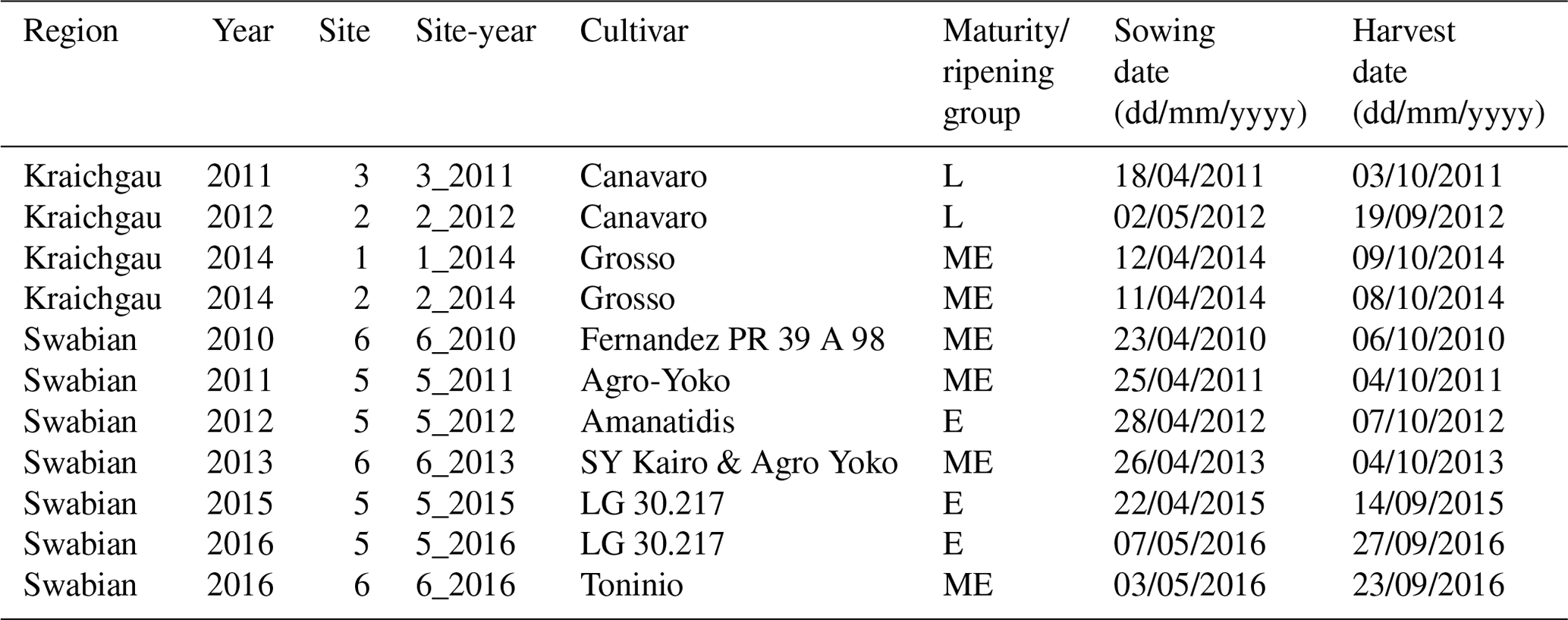
At every study site, which had an area of approx. 15 ha, replicate observations were made by assessing phenological development stages from maize plants in five subplots of 2 m × 2 m each. Ten maize plants were chosen from each subplot. We used the BBCH growth stage code (Meier, 1997) to define the development stages. The BBCH value of 10 marks the emergence and the start of leaf development, 30 stands for stem elongation, 50 for inflorescence, emergence or heading, 60 for flowering or anthesis, 70 for development of fruit, 80 for ripening, and 90 for senescence (Fig. 1ii). In the following sections, the individual growing seasons for silage maize are denoted by the site and year of growth, i.e. the site-year (Table 1). For example, silage maize grown at site 2 in Kraichgau in the year 2012 is referred to as “2_2012”. The different cultivars used in the study can be grouped into three ripening or maturity groups, based on their timing of ripening. Mid-early (ME) and late (L) ripening cultivars were grown in Kraichgau, and early (E) and mid-early (ME) ripening cultivars were grown on the Swabian Alb.

Table 1 Early (E), mid-early (ME), and late (L) ripening cultivars of silage maize, with their sowing and harvest dates, grown at the study sites in Kraichgau (sites 1, 2, and 3) and the Swabian Alb (sites 5 and 6) between 2010 and 2016.

2.2 Soil–crop model

To simulate the soil–crop system, we used the SPASS crop growth model (Wang, 1997). SPASS is implemented in the Expert-N 5.0 (XN5) software package (Heinlein et al., 2017; Klein et al., 2017; Priesack, 2006). In XN5, the SPASS crop model is coupled with the Richards equation for soil–water movement as implemented in the Hydrus-1D model (Šimůnek et al., 1998). The routine uses van Genuchten–Mualem hydraulic functions (van Genuchten, 1980; Mualem, 1976) and the heat transfer scheme from the Daisy model (Hansen et al., 1990). In the SPASS model, germination to emergence (up to BBCH 10), the vegetative phase (between BBCH 10 and 60), and the generative or reproductive phase (BBCH 61 onwards) of the crop are modelled. Temperature and photoperiod are the two main factors affecting the phenological development rate (for details, refer to Appendix A: SPASS phenology model).

Daily weather data consisting of maximum and minimum temperatures were used in XN5 to calculate the air temperatures within the crop canopy. Soil properties (texture class, grain size, rock fraction, bulk density, porosity), as well as van Genuchten parameters and hydraulic properties (soil water content at wilting point, field capacity, residual and saturated water content, and saturated hydraulic conductivity), were based on soil samples taken at the sites in 2008 to characterize the soil profile. The soil horizons in the model were based on these soil profile descriptions. Initial values of soil volumetric water content were based on measurements. The simulations for each site-year were started on the harvest date of the preceding crop in the crop rotation at that site. This ensured adequate spin-up time prior to the simulation of silage maize, which was sown in April and May.

2.3 Selection of model parameters

Parameters were pre-selected (Hue et al., 2008; Makowski et al., 2006) based on expert knowledge. The prior default values and uncertainty ranges are given in Table 2. A global sensitivity analysis using the Morris method (Morris, 1991) was then carried out to identify the sensitive parameters to be estimated through Bayesian calibration (Supplement S1). The sensitive parameters identified for calibration were: effective sowing depth (SOWDEPTH), which influences the emergence rate, and parameters affecting development in the vegetative phase (PDD1, TMINDEV1, DELTOPT1, and DELTMAX1). Parameter DELTOPT2, from the temperature response function during the reproductive phase, was estimated during calibration even though it was less sensitive. The choice of using this parameter during calibration was based on knowledge of model behaviour, so as to reduce the calibration error in the reproductive phase (Lamboni et al., 2009). Thus, out of 11 pre-selected parameters (Table 2), six were estimated in BSU, while the remaining parameters were fixed at their default values.

Table 2 SPASS model parameters for phenological development. The default values and two standard deviations (± 2 SD) were based on expert knowledge. “Status in calibration” indicates the parameters which were estimated or fixed to the default value during Bayesian calibration. Minimum (min) and maximum (max) values were set for estimated parameters to constrain the prior parameter ranges to reasonable values during calibration.

2.4 Bayesian sequential updating

In the BSU approach, Bayesian calibration is applied in a sequential manner. New data are used to re-calibrate the model, conditional on the prior information from previously gathered data. We describe the details of this approach here.

Bayes theorem states that the posterior probability of parameters θ given the data Y, P(θ|Y), is proportional to the product of the joint prior probability of the parameters P(θ) and the probability of generating the observed data with the model, given the parameters P(Y|θ). The term P(Y|θ) is referred to as the likelihood function and is defined as the likelihood that observation Y , that is observed phenological development in this study, is generated by the model using the parameter vector θ. The posterior probability distribution is obtained by normalizing this product by the prior predictive distribution (Gelman et al., 2013) or Bayesian model evidence (Schöniger et al., 2015) P(Y), which is obtained by integrating the product over the entire parameter space.

Hence, we write:

$$\begin{array}{}\text{(1)}& P\left(\mathit{\theta }|\mathit{Y}\right)={\displaystyle \frac{P\left(\mathit{\theta }\right)P\left(\mathit{Y}\right|\mathit{\theta })}{P\left(\mathit{Y}\right)}},\end{array}$$

where

$$\begin{array}{}\text{(2)}& P\left(\mathit{Y}\right)={\int }_{\mathit{\theta }}P\left(\mathit{\theta }\right)P\left(\mathit{Y}|\mathit{\theta }\right)\mathrm{d}\mathit{\theta }.\end{array}$$

Equation (2) can become intractable, especially with a large number of parameters as this involves integrating over high-dimensional space (Schöniger et al., 2015). Instead, sampling methods such as Markov chain Monte Carlo (MCMC) are used to estimate the posterior distribution.

For one site-year sy₁ and corresponding observation vector ${\mathit{Y}}_{{\mathrm{sy}}_{\mathrm{1}}}$, the posterior parameter probability distribution is

$$\begin{array}{}\text{(3)}& P\left(\mathit{\theta }|{\mathit{Y}}_{{\mathrm{sy}}_{\mathrm{1}}}\right)={\displaystyle \frac{P\left(\mathit{\theta }\right)P\left({\mathit{Y}}_{{\mathrm{sy}}_{\mathrm{1}}}|\mathit{\theta }\right)}{{\int }_{\mathit{\theta }}P\left(\mathit{\theta }\right)P\left({\mathit{Y}}_{{\mathrm{sy}}_{\mathrm{1}}}|\mathit{\theta }\right)\mathrm{d}\mathit{\theta }}},\end{array}$$

where P(θ) represents the initial prior probability distribution that could be based on expert knowledge. The posterior parameter distribution $P\left(\mathit{\theta }|{\mathit{Y}}_{{\mathrm{sy}}_{\mathrm{1}}}\right)$ can now be used as a prior distribution for the next site-year sy₂. Thus, for site-year sy_n with an observation vector ${\mathit{Y}}_{{\mathrm{sy}}_n}$, the posterior parameter probability distribution is

$$\begin{array}{}\text{(4)}& P\left(\mathit{\theta }|{\mathit{Y}}_{{\mathrm{sy}}_n}\right)={\displaystyle \frac{P\left(\mathit{\theta }|{\mathit{Y}}_{{\mathrm{sy}}_{(n-\mathrm{1})}}\right)P\left({\mathit{Y}}_{{\mathrm{sy}}_n}|\mathit{\theta }\right)}{{\int }_{\mathit{\theta }}P\left(\mathit{\theta }|{\mathit{Y}}_{{\mathrm{sy}}_{(n-\mathrm{1})}}\right)P\left({\mathit{Y}}_{{\mathrm{sy}}_n}|\mathit{\theta }\right)\mathrm{d}\mathit{\theta }}}.\end{array}$$

This equation defines the BSU approach in which the model is calibrated in a sequential manner. New data from a site-year (${\mathit{Y}}_{{\mathrm{sy}}_n}$) are used to re-calibrate the model, conditional on the prior information from previous site-years. The posterior distribution obtained from the previous Bayesian calibration $P\left(\mathit{\theta }\right|{\mathit{Y}}_{{\mathrm{sy}}_{(n-\mathrm{1})}}$) is used as prior probability for calibration to the next site-year.

With the aim of making the computations tractable, we deviate slightly from this pure BSU approach as we do not strictly use the posterior distribution from the previous site-year as the prior distribution for the next one, but sequentially calibrate the model to data from an increasing number of site-years instead. The reason for this deviation is that in applying BSU, where the posterior parameter distribution is estimated by sampling methods, a probability density function needs to be approximated from the sample, so that it can be used as a prior probability for the subsequent site-year. This approximation introduces additional errors. Since joint inference is known to be better than sequential inference using posterior approximations (Thijssen and Wessels, 2020), Eq. (4) can be re-written, under the assumption that the phenology observations from all site-years are independent and identically distributed (Gelman et al., 2013), as follows:

$$\begin{array}{}\text{(5)}& P\left(\mathit{\theta }|{\mathit{Y}}_{{\mathrm{sy}}_n}\right)={\displaystyle \frac{P\left(\mathit{\theta }\right){\prod }_{x={\mathrm{sy}}_{\mathrm{1}}}^{{\mathrm{sy}}_n}P\left({\mathit{Y}}_x|\mathit{\theta }\right)}{{\int }_{\mathit{\theta }}P\left(\mathit{\theta }\right){\prod }_{x={\mathrm{sy}}_{\mathrm{1}}}^{{\mathrm{sy}}_n}P\left({\mathit{Y}}_x|\mathit{\theta }\right)\mathrm{d}\mathit{\theta }}}.\end{array}$$

Thus, we use Eq. (5) to sequentially update the probability distribution of parameters by increasing the dataset size at each step through the addition of one site-year worth of new data Y_x to the previous dataset Y_x−1.

After each inferential step, the probability of observing a certain phenology at the next site-year sy_n+1 is predicted by

$$\begin{array}{}\text{(6)}& P\left({\mathit{Y}}_{{\mathrm{sy}}_{n+\mathrm{1}}}|{\mathit{Y}}_{{\mathrm{sy}}_n}\right)=\int P\left({\mathit{Y}}_{{\mathrm{sy}}_{n+\mathrm{1}}}|\mathit{\theta }\right)P\left(\mathit{\theta }|{\mathit{Y}}_{{\mathrm{sy}}_n}\right)\mathrm{d}\mathit{\theta },\end{array}$$

where $P\left({\mathit{Y}}_{{\mathrm{sy}}_{n+\mathrm{1}}}|{\mathit{Y}}_{{\mathrm{sy}}_n}\right)$ is the posterior predictive distribution (Gelman et al., 2013). We refer to the current methodology as BSU, although it is not strictly so, for reasons of simplicity and the formal similarity of our approach. All calculations and the BSU were carried out using the R programming language (R Core Team, 2020).

In the following sections, we describe the components of Bayes formula in detail.

2.4.1 Likelihood function

Let $\mathit{\theta }=({\mathit{\phi }}_{\mathrm{1}}{\mathit{\phi }}_{\mathrm{2}}{\mathit{\phi }}_{\mathrm{3}},\mathrm{\dots }{\mathit{\phi }}_j)$ represent a vector of the model parameters to be estimated in this study (Table 2). Suppose $\mathit{Y}=({\stackrel{\mathrm{‾}}{y}}_{\mathrm{1}},{\stackrel{\mathrm{‾}}{y}}_{\mathrm{2}},{\stackrel{\mathrm{‾}}{y}}_{\mathrm{3}},\mathrm{\dots }{\stackrel{\mathrm{‾}}{y}}_d$) is a vector of the means of observed phenological development on different days during the growing season for a particular site-year. The mean observation ${\stackrel{\mathrm{‾}}{y}}_d$ on day d for the site-year is given by

$$\begin{array}{}\text{(7)}& {\stackrel{\mathrm{‾}}{y}}_d={\displaystyle \frac{\mathrm{1}}{P}}{\displaystyle \frac{\mathrm{1}}{R}}\sum _{p=\mathrm{1}}^P\sum _{r=\mathrm{1}}^R{y}_{r,p,d},\end{array}$$

where $y_{r,p,d}$ represents the rth replicate of observed phenological development, measured at subplot p on day d for a particular site-year, R is the total number of replicates at subplot p, and P is the total number of subplots per field.

If we assume that all replicates R in all subplots P are independent, the standard deviation of the replicate observations on day d is ${\mathit{\sigma }}_{r,p,d}=\sqrt{\sum _{p=\mathrm{1}}^P\sum _{r=\mathrm{1}}^R{\left(y_{r,p,d}-{\stackrel{\mathrm{‾}}{y}}_d\right)}^{\mathrm{2}}/(P\times R)}$ . This is one source of observation error that represents the spatial variability at the study site which is below the spatial resolution of the model. We also assume an additional source of error in identification of the correct phenological stage and its exact timing of occurrence. We assume that this error is within a standard deviation of 2 BBCH (${\mathit{\sigma }}_{\mathrm{ident},d}=\mathrm{2}$ for each observation day d). This assumption was made because 2 is the most common difference between development stages in the phenological development of maize on the BBCH scale. Assuming that the error from replicate observations (${\mathit{\sigma }}_{r,p,d}$) and the error in the identification of phenological stages are additive, the total observation error is ${\mathit{\sigma }}_d^{\mathrm{2}}={\left({\mathit{\sigma }}_{r,p,d}+{\mathit{\sigma }}_{\mathrm{ident},d}\right)}^{\mathrm{2}}$.

The model residual ${\stackrel{\mathrm{‾}}{y}}_d-f(\mathit{\theta }{)}_d$ is the difference between the observed ${\stackrel{\mathrm{‾}}{y}}_d$ and the model simulated f(θ)_d phenological stage and is represented by the likelihood function. Assuming normally distributed residuals, it is given by

$$\begin{array}{}\text{(8)}& P\left({\stackrel{\mathrm{‾}}{y}}_d|\mathit{\theta }\right)={\displaystyle \frac{\mathrm{1}}{{\mathit{\sigma }}_d\sqrt{\mathrm{2}\mathit{\pi }}}}{e}^{-\mathrm{0.5}{\left(\frac{{\stackrel{\mathrm{‾}}{y}}_d-f{\left(\mathit{\theta }\right)}_d}{{\mathit{\sigma }}_d}\right)}^{\mathrm{2}}}.\end{array}$$

The likelihood values for all the observations are combined by taking the product of the likelihoods per day of observation, under the assumption of independent and identically distributed model residuals. Thus, the joint likelihood function is given by

$$\begin{array}{}\text{(9)}& P\left({\mathit{Y}}_x|\mathit{\theta }\right)=\prod _{d=\mathrm{1}}^{D}P\left({\stackrel{\mathrm{‾}}{y}}_d|\mathit{\theta }\right),\end{array}$$

where Y_x is the observation vector for site-year x.

2.4.2 Prior probability distribution

As prior information, we used a weakly informative probability distribution function (pdf) to ensure that the posterior parameter distributions are mainly determined by the data that are sequentially incorporated. For this, we used a platykurtic prior probability distribution that is a convolution of a uniform and a normal distribution (Fig. D1) of the form:

$$\begin{array}{}\text{(10)}& P\left({\mathit{\phi }}_j\right)=\left\{\begin{array}{ll}\frac{\mathrm{1}}{c}\frac{\mathrm{1}}{\mathit{\sigma }\sqrt{\mathrm{2}\mathit{\pi }}}{e}^{-\frac{{\left({\mathit{\phi }}_j-\mathit{\mu }\right)}^{\mathrm{2}}}{\mathrm{2}{\mathit{\sigma }}^{\mathrm{2}}}}& \text{for}a\le {\mathit{\phi }}_j<\mathit{\mu }-\mathrm{2}\mathit{\sigma }\\ \frac{\mathrm{1}}{c}\frac{\mathrm{1}}{\mathit{\sigma }\sqrt{\mathrm{2}\mathit{\pi }}}{e}^{-\mathrm{2}}& \text{for}\mathit{\mu }-\mathrm{2}\mathit{\sigma }\le {\mathit{\phi }}_j\le \mathit{\mu }+\mathrm{2}\mathit{\sigma }\\ \frac{\mathrm{1}}{c}\frac{\mathrm{1}}{\mathit{\sigma }\sqrt{\mathrm{2}\mathit{\pi }}}{e}^{-\frac{{\left({\mathit{\phi }}_j-\mathit{\mu }\right)}^{\mathrm{2}}}{\mathrm{2}{\mathit{\sigma }}^{\mathrm{2}}}}& \text{for}\mathit{\mu }+\mathrm{2}\mathit{\sigma }<{\mathit{\phi }}_j\le b\end{array}\right).\end{array}$$

where φ_j is a model parameter in the parameter vector θ, a and b are the minimum and maximum limit for the parameter, respectively, μ is the mean (default value in Table 2), and σ is the standard deviation. The normalization constant c is used to ensure that the area under the curve equals unity as required for probability density functions.

$$\begin{array}{}\text{(11)}& \begin{array}{rl}c& =-\mathrm{erf}\left(\sqrt{\mathrm{2}}\right)+{\displaystyle \frac{\mathrm{4}}{\sqrt{\mathrm{2}\mathit{\pi }}}}{e}^{-\mathrm{2}}-{\displaystyle \frac{\mathrm{1}}{\mathrm{2}}}\mathrm{erf}\left({\displaystyle \frac{a-\mathit{\mu }}{\mathit{\sigma }\sqrt{\mathrm{2}}}}\right)\\ & +{\displaystyle \frac{\mathrm{1}}{\mathrm{2}}}\mathrm{erf}\left({\displaystyle \frac{b-\mathit{\mu }}{\mathit{\sigma }\sqrt{\mathrm{2}}}}\right).\end{array}\end{array}$$

The joint prior pdf was calculated by $P\left(\mathit{\theta }\right)={\prod }_{j=\mathrm{1}}^{J}P\left({\mathit{\phi }}_j\right)$ and the model parameters were assumed to be uncorrelated. The parameters a, b, σ, μ, of P(φ_j) were based on expert knowledge (Table 2).

2.4.3 Posterior probability distribution

The posterior parameter distribution was sampled using the Markov chain Monte Carlo method – Metropolis algorithm (Metropolis et al., 1953) (for details, refer to Appendix B: Posterior sampling using MCMC Metropolis algorithm). Three chains were run in parallel. A normal distribution was chosen as the transition kernel. The jump size was adapted so that the acceptance rate would be between 25 % and 35 % (Gelman et al., 1996; Tautenhahn et al., 2012). For each sequential update calibration case, when a new site-year was added to the calibration sequence, the three chains were re-initialized and the transition kernel was re-tuned. A preliminary calibration test case, in which the model was calibrated to site-year 6_2010, was used to generate the starting points of the chains for each of the calibration cases. The starting points were randomly sampled from the posterior parameter range of the calibrated test case. This was done to reduce the time to convergence. For the test case calibration, the starting points of the chains were randomly sampled from the prior range. The number of iterations for adapting the transition kernel varied between the different calibration cases. This number was low for some of the calibration cases because we set the initial pre-adaptation value for the standard deviation of the transition kernel, so that the acceptance rate would be between 25 % and 35 %. This initial value was based on knowledge gained from preliminary calibration test simulations. Convergence of the chains after jump adaptation was checked using the Gelman–Rubin convergence diagnostic (Brooks and Gelman, 1998; Gelman and Rubin, 1992). The total number of samples of the posterior distribution in each calibration case was dependent on the Gelman–Rubin diagnostic being ≤ 1.1, while ensuring a minimum of 500 accepted samples per chain, that is a minimum of 1500 samples across the three chains. In effect, the total number of samples per calibration case was greater than 1500. The burn-in was variable and depended on the jump adaptation. Only the iterations from the jump adaptation step were discarded as burn-in. Parameter mixing was evaluated using trace plots.

For model validation, the posterior predictive distribution was used to simulate phenological development and compare it with observations at site-years that were not included in the calibration sequence.

2.5 Performance metrics

Bias and normalized root mean square error (NRMSE), as defined in Eqs. (12) and (13), for site-year sy were calculated to assess the calibration and prediction performance.

$$\begin{array}{}\text{(12)}& {\displaystyle }{\mathrm{Bias}}_{\mathrm{sy}}={\displaystyle \frac{\mathrm{1}}{D}}\sum _{d=\mathrm{1}}^D\left({\stackrel{\mathrm{‾}}{y}}_d-f{\left({\mathit{\theta }}_i\right)}_d\right)\text{(13)}& {\displaystyle }{\mathrm{NRMSE}}_{\mathrm{sy}}=\sqrt{{\displaystyle \frac{\mathrm{1}}{D}}\sum _{d=\mathrm{1}}^D{\displaystyle \frac{{\left({\stackrel{\mathrm{‾}}{y}}_d-f{\left({\mathit{\theta }}_i\right)}_d\right)}^{\mathrm{2}}}{{\mathit{\sigma }}_d^{\mathrm{2}}}}}\end{array}$$

Here, θ_i is the ith parameter vector, D is the total number of observation days for the particular site-year, f(θ_i)_d is the simulated phenological development, ${\stackrel{\mathrm{‾}}{y}}_d$ is the mean observed phenological development, and σ_d is the standard deviation of the observations (as defined in Sect. 2.4.1 Likelihood function) on day d. Under the assumption of normally distributed error, the natural logarithm of the likelihood probability is inversely proportional to the normalized mean square error: $\ln \left(P\left({\mathit{Y}}_{\mathrm{sy}}|{\mathit{\theta }}_i\right)\right)\propto -{{\mathrm{NRMSE}}_{\mathrm{sy}}}^{\mathrm{2}}$. The normalized bias ${\mathrm{NBias}}_{\mathrm{sy}}=\frac{\mathrm{1}}{D}{\sum }_{d=\mathrm{1}}^D\frac{{\stackrel{\mathrm{‾}}{y}}_d-f{\left({\mathit{\theta }}_i\right)}_d}{{\mathit{\sigma }}_d}$ is also reported in some plots.

The prediction quality is good when NRMSE is low and bias is zero. Prediction performance is classified as good, moderate, or poor depending on the median NRMSE of the predictions for a site-year. We use the following categories: good performance for median NRMSE ≤ 1, moderate for 1 < median NRMSE ≤ 2, poor for 2 < median NRMSE ≤ 3 and very poor for median NRMSE > 3.

We estimated the information entropy of the posterior parameter distributions after each sequential update using the redistribution estimate equation (Beirlant et al., 1997) (Supplement S2). A change in entropy with sequential updates indicates a change in uncertainty of the parameters, where higher information entropy indicates greater uncertainty in the posterior parameters. In line with our hypotheses, we expect the entropy to decrease with sequential updates.

2.6 Modelling cases

The BSU approach described in the previous sections and the subsequent analysis using the performance metrics were applied to two synthetic sequences and two true sequences of site-years. The synthetic sequences were used to demonstrate the application of the BSU approach in ideal conditions, while the true sequences were used to extend the application to real-world conditions. Figure 2 shows the four sequences and the site-years used for calibration and validation.

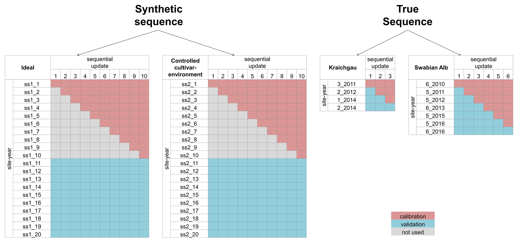
Figure 2 The site-years used for calibration and validation in each sequential update for the two synthetic sequences, namely ideal and controlled cultivar–environment, and the two true sequences for Kraichgau and the Swabian Alb are shown. In the synthetic sequences, a total of 10 updates were performed by sequentially adding 1 through 10 site-years to the calibration dataset. After each update, prediction quality was analysed for a set of 10 validation site-years. A total of three sequential updates in Kraichgau and six sequential updates in the Swabian Alb true sequences were analysed. In the sequential updates for the true sequences, a site-year was included for calibration, following the actual chronological order of growth. The remaining site-years grown in the region were then used for validation.

2.7 Synthetic sequences

We set up two synthetic sequences, namely ideal and controlled cultivar–environment. In each synthetic sequence, we used 10 sequential updates wherein 1 through 10 site-years were used in calibration. After each sequential update, the calibrated model was validated against a different set of 10 synthetic site-years (Fig. 2). Note here that the 10 site-years used for validation were the same across the sequential updates. Data from the 10 site-years used for calibration and the 10 site-years used for validation for the two synthetic sequences are shown in Fig. 3. Site-year 6_2010 was used to generate data for the synthetic sequences, as described here.

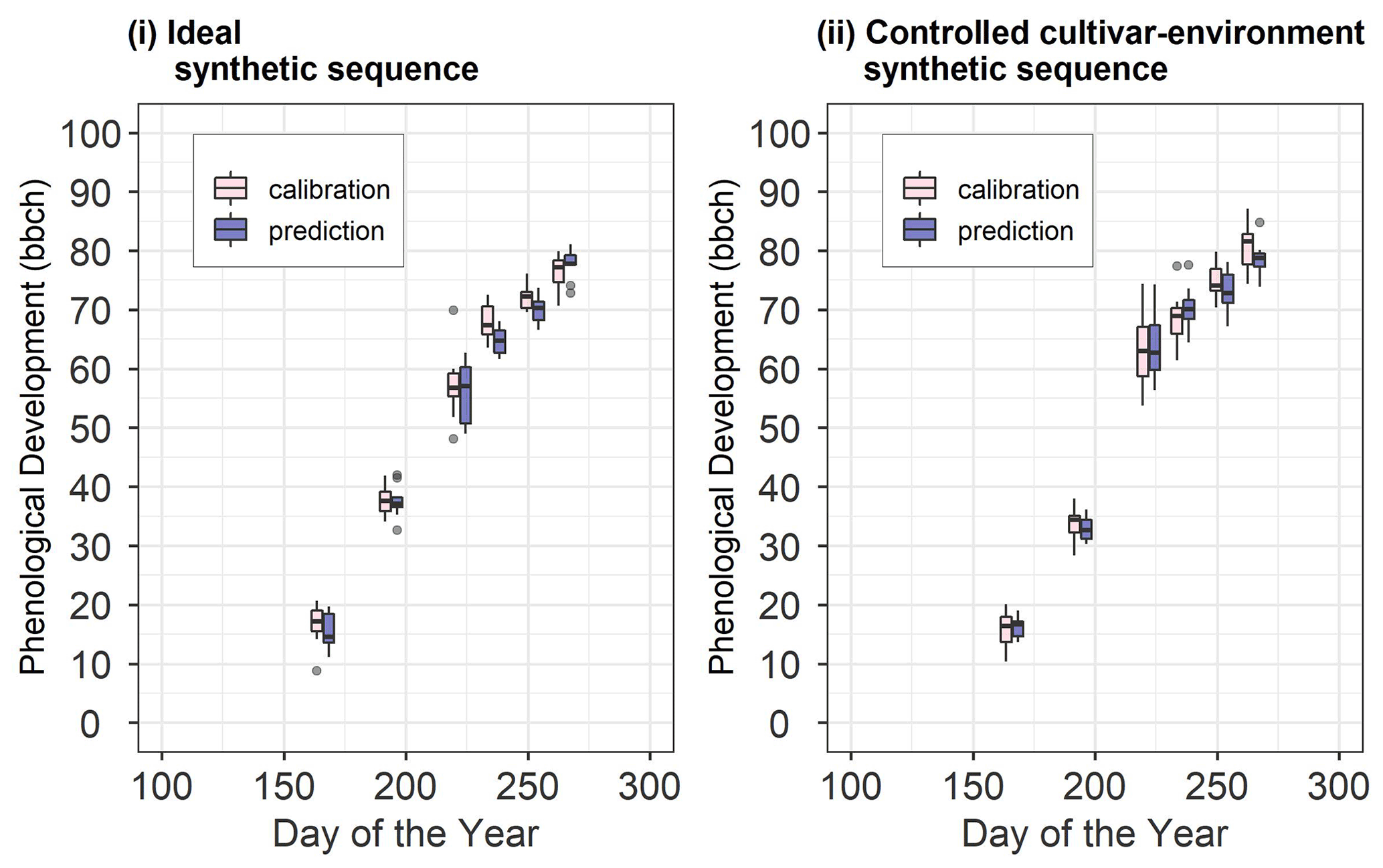
Figure 3 Synthetic site-year observations used for calibration and prediction in (i) the ideal and (ii) controlled cultivar–environment synthetic sequences. The pink boxes and whiskers represent the range of values for the 10 synthetic site-years used for calibration while the blue boxes and whiskers represent the range of values for the 10 site-years used for validation. The length of the box represents the inter-quartile range (IQR), whiskers extend from the box up to 1.5× IQR and values beyond this range are plotted as points.

The ideal sequence represents a case in which the model is able to accurately simulate the observations. The only sources of difference between site-years are from the spatial variability at the field site which is below model resolution and from the incorrect identification of phenological stages during field observations. To generate the ideal sequence of site-years, we first calibrated the model to phenology at 6_2010. The parameter set θ_MAP corresponding to the maximum a posteriori probability (MAP) estimate was used to simulate phenology and generate the synthetic dataset. To introduce inter-site-year differences, noise was added to simulated phenology f(θ_MAP)_d on observation day d, where the noise was equal to the total observation uncertainty σ_d on that day for site-year 6_2010. Thus, for each synthetic site-year on observation day d, the phenological development was sampled from the range of total observation uncertainty σ_d at 6_2010, around simulated phenology f(θ_MAP)_d . The synthetic observations were generated for the same observation days as the actual observations at 6_2010. We ensured that phenological development stages did not decrease with time, that is ${\dot{y}}_d\ge {\dot{y}}_{d-\mathrm{1}}$, where ${\dot{y}}_{d-\mathrm{1}}$ is the sampled phenological development on the previous observation day d−1. Of the 20 site-years generated in this manner, 10 site-years were used for calibration while the remaining 10 were used for validation. The synthetic site-years were ordered randomly during BSU calibration.

The controlled cultivar–environment sequence represents a sequence of site-years where the same cultivar is grown under the same environmental conditions. In this case, however, the model may not accurately simulate the observations, implying the presence of model structural error (e.g. the model's inability to capture slow emergence as explained in Appendix A: SPASS phenology model). For the controlled cultivar–environment sequence, we generated the synthetic site-year data from observations of the cultivar grown at 6_2010. For each synthetic site-year, the phenological development ${\dot{y}}_d$ on observation day d was sampled from the range of total observation uncertainty σ_d around the observed mean ${\stackrel{\mathrm{‾}}{y}}_d$. As in the ideal sequence, we ensured that phenological development stages did not decrease with time. Again, 10 site-years were randomly assigned for calibration.

2.7.1 True sequences

A total of three sequential updates in Kraichgau and six sequential updates in the Swabian Alb were analysed (Fig. 2). In each sequential update, an additional site-year was included in the calibration dataset, following the actual chronological order in which maize was grown in the regions. For the Kraichgau sequence, four site-years were available for calibration and validation (3_2011, 2_2012 1_2014, and 2_2014). The model was sequentially calibrated to phenological development of maize for site-years 3_2011, 2_2012, and 1_2014. After each update, phenological development was predicted for the subsequent site-years. For example, in the first sequential update at Kraichgau, the model was calibrated to 3_2011. The site-years 2_2012, 1_2014 ,and 2_2014 were used for validation to assess the prediction quality of the calibrated model. In the second sequential update, the model was calibrated to 3_2011 and 2_2012, while 1_2014 and 2_2014 were used for validation. Note here that the number of site-years used for validation decreases with each sequential update. In the Swabian Alb sequence, seven site-years were available for sequential calibration and validation (6_2010, 5_2011, 5_2012, 6_2013, 5_2015, 5_2016, and 6_2016). The sequential updates were performed in a similar manner as in Kraichgau.

3 Results

In this section, we first describe the results for one example of Bayesian calibration using the data from site-year 6_2010 (Sect. 3.1 Bayesian calibration results). Here, we examine the resulting simulated phenology after calibration as well as the posterior parameter distributions. We then look at the results from the synthetic and true sequences. We first evaluate the evolution of the posterior parameter distributions with sequential updates. As an example, we analyse the marginal distributions of the individual parameters and entropy of the joint parameter distributions for the true sequences (Sect. 3.2 Parameter uncertainty). Lastly, we report the prediction quality results for the synthetic and true sequences (Sect. 3.3 Prediction quality).

3.1 Bayesian calibration results

By way of example, Fig. 4 shows the Bayesian phenological model calibration results for silage maize for the first site-year 6_2010. Cross-plots of the posterior parameters (Fig. 4i) show a weak negative correlation between PDD1 and TMINDEV1 and between PDD1 and DELTOPT1, while a weak positive correlation is observed between PDD1 and DELTMAX1. The observed mean phenological development falls within the range of simulations after calibration (Fig. 4ii). The marginal posterior parameter distributions are narrower than the initial prior distributions (Fig. 4iii). A shift in parameter distribution to the margins of the prior ranges is also noteworthy.

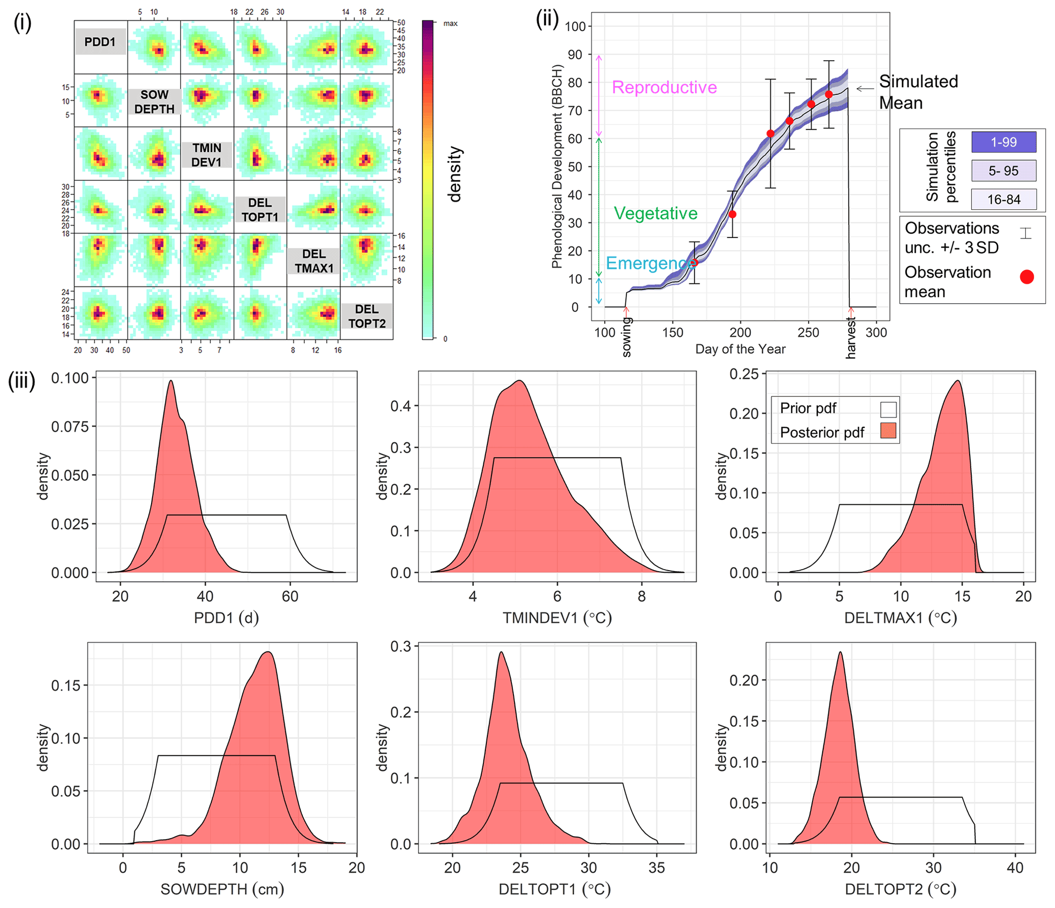
Figure 4 Results of Bayesian calibration of the model to phenological development (BBCH stages) for site-year 6_2010. (i) Cross-plot of the posterior samples of the six estimated parameters. Red represents high density and blue low density (IDPmisc package in R, Locher, 2020). (ii) Observed and simulated phenological development after calibration, plotted against the day of the year. The red points are the mean observations, while the black error bars indicate ± 3 SDs. The mean simulation is indicated by the continuous black line. The blue bands represent the different percentiles of simulated phenology. Note that the simulated phenology bands only represent the uncertainty in model parameters and do not include the noise term. (iii) Prior (white) and posterior (salmon) marginal parameter distributions for the six estimated parameters.

3.2 Parameter uncertainty

We analysed the change in posterior parameter distribution with the sequential updates. Figure 5i shows the marginal initial prior and posterior parameter distributions for the Swabian Alb and Kraichgau true sequences. The x-axis from left to right indicates the initial prior parameter distribution followed by the sequential calibration of the model to an increasing number of site-years. The distributions for the six estimated parameters are compared after each sequential update. The width of each box with whiskers represents the uncertainty in the parameter values. There is a clear narrowing of parameter distributions after the first sequential update from the initial prior. However, with the exception of DELTOPT2, the remaining parameters do not show a noticeable and consistent narrowing in range with sequential updates. Information entropy of the joint posterior parameter distributions in Fig. 5ii decreases with sequential updates and there is a large reduction in entropy with the first sequential update. In the Swabian Alb sequence (Fig. 5iia), entropy continues to decrease until the model is calibrated to 6_2010, 5_2011, and 5_2012, after which there is no significant reduction. In the Kraichgau sequence (Fig. 5iib), the inclusion of 1_2014 during calibration results in further uncertainty reduction. Similar observations were made for the synthetic sequences (Supplement S6).

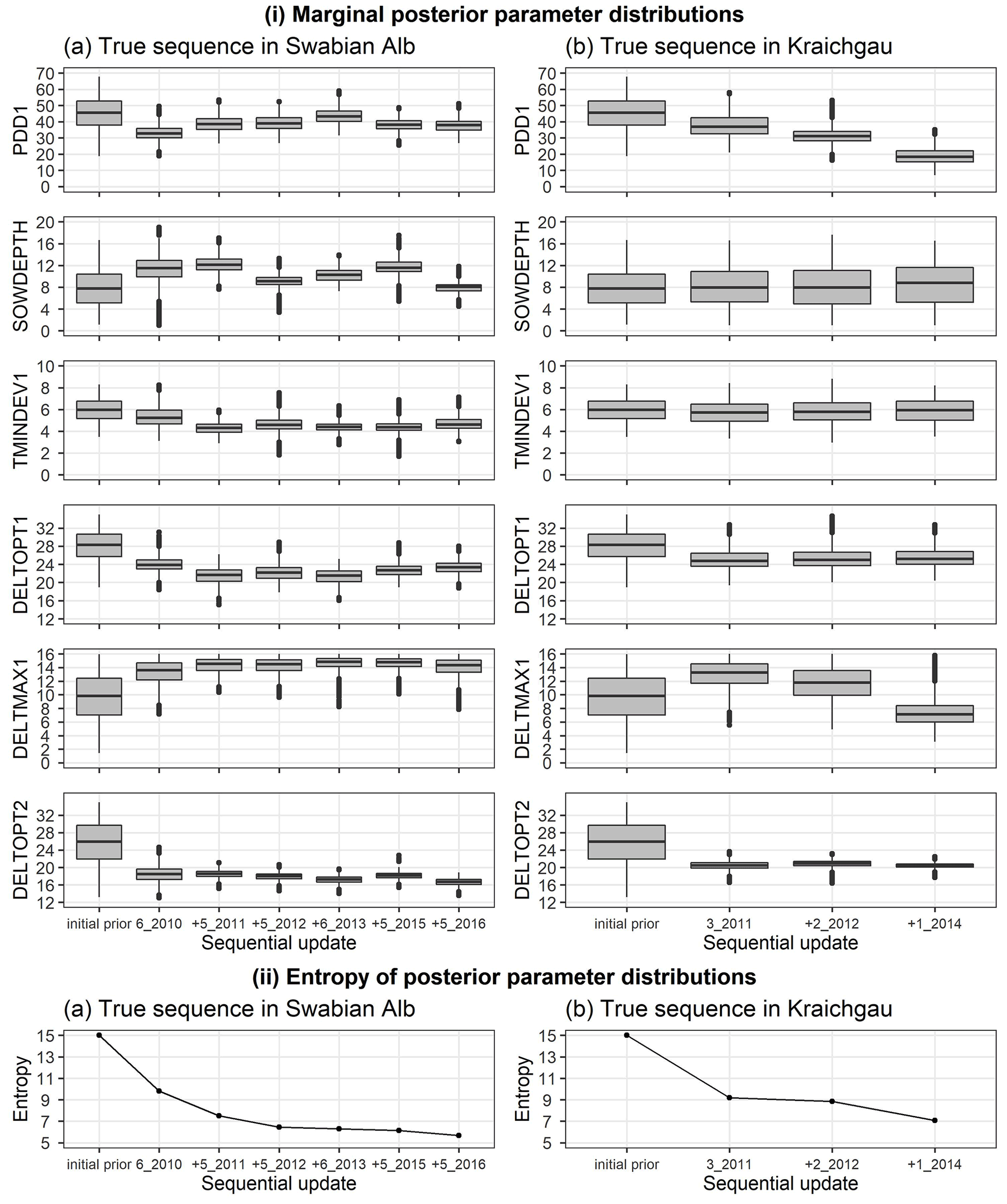
Figure 5 (i) Marginal initial prior and posterior parameter distributions of the six estimated parameters plotted against the calibration site-years, after BSU was applied to a true sequence (a) on the Swabian Alb and (b) in Kraichgau. The SPASS model was calibrated to observed phenological development (BBCH). (ii) Information entropy of the joint posterior parameter distributions plotted against the calibration site-years, after BSU was applied to the true sequences. The x-axis labels from left to right indicate the initial prior parameter distribution followed by the sequential calibration of the model to an increasing number of site-years. The “+” symbol before the site-year label on the x-axis indicates the new site-year that was included in the sequential calibration. The length of the box in (i) represents the inter-quartile range (IQR), whiskers extend from the boxes up to 1.5× IQR and values beyond this range are plotted as points.

3.3 Prediction quality

3.3.1 Synthetic sequences

In the synthetic sequences, we assessed the prediction quality after applying BSU to 10 synthetic site-years, while excluding model structural error and inter-site-year differences in cultivar and environmental conditions in the ideal sequence and controlled cultivar–environment sequence, respectively. In both sequences we account for identification uncertainty and spatial variability within the modelled site. Figure 6 shows the trend in median NRMSE and bias with the sequential updates from 1 to 10, for the two synthetic sequences. While the bias and NRMSE were calculated for all parameter vectors in the posterior sample derived from the MCMC sampling method, only the median values are plotted and analysed for simplicity.

In the ideal sequence (Fig. 6i), the overall median NRMSE (Fig. 6ia) and bias (Fig. 6ib) are low, with many site-years exhibiting a drop in the median NRMSE below a value of 1. However, after a few sequential updates, no further reduction is observed. In the controlled cultivar–environment sequence (Fig. 6ii), although most individual site-years showed a reduction in median NRMSE with the sequential updates, there were some that exhibited an increase in median NRMSE (ss2_12 and ss2_15 in Fig. 6iia). These site-years were also characterized by low initial median prediction bias, followed by an increase in the absolute bias with sequential updates (Fig. 6iib).

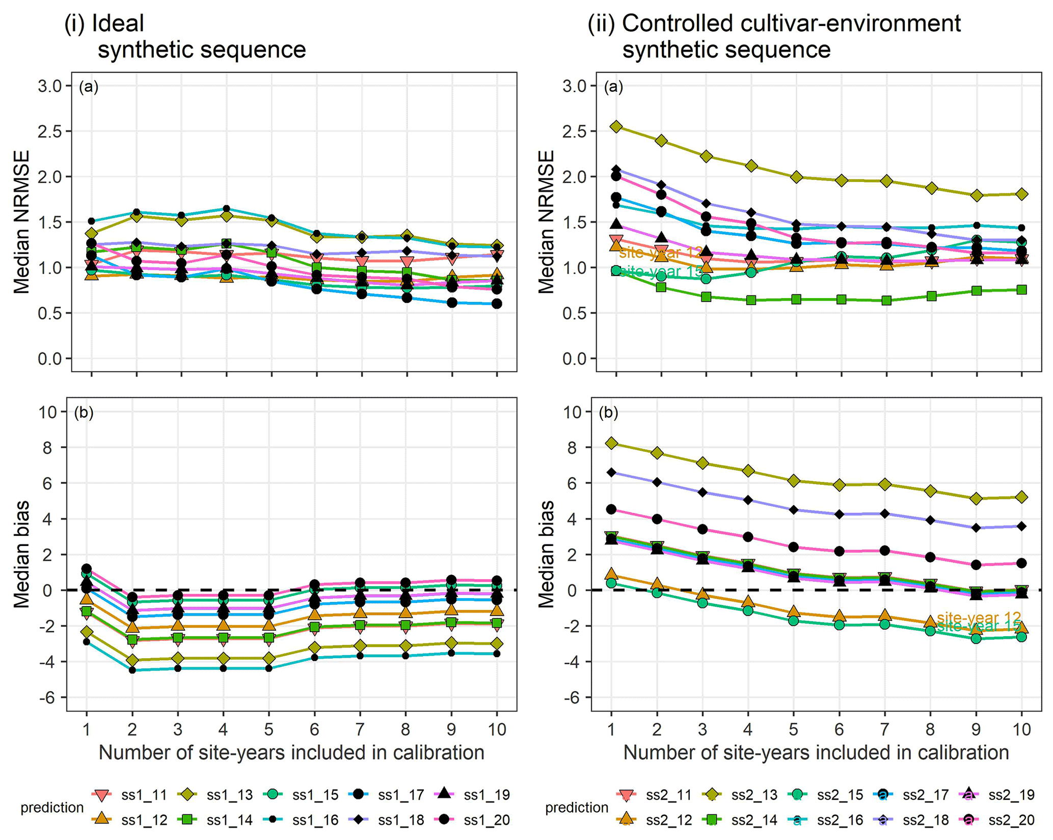
Figure 6 (a) Median NRMSE and (b) median bias of prediction for the 10 validation site-years, after BSU was applied to the ideal (i) and controlled cultivar–environment (ii) synthetic sequences. The number of site-years used for calibration is shown on the x-axis and represents the sequential updates from 1 to 10. The SPASS model was calibrated to phenological development (BBCH). The lines and points correspond to the 10 synthetic validation site-years: ss1_11-ss1_20 from the ideal sequence and ss2_11-ss2_20 from the controlled cultivar–environment sequence.

3.3.2 True sequences

Because fewer site-years were used for validation in the true sequence as compared to the synthetic sequence, we analysed the prediction quality for each validation site-year individually, with the sequential updates. Figure 7 shows the prediction quality (i.e. NRMSE and bias for all the posterior predictive samples) of the model after BSU was applied to the true sequence of site-years in Kraichgau (Fig. 7i–iii) and on the Swabian Alb (Fig. 7iv–ix). For each site-year, we plot the quality of prediction, after calibration to all preceding site-years. For example, Fig. 7vi shows the performance metric for site-year 6_2013 after the model was calibrated first to 6_2010, then to 6_2010 and 5_2011, and finally to 6_2010, 5_ 2011, and 5_2012, respectively (blue box-plots from left to right). As a reference, the performance metric derived from calibrating the model to the target site-year, namely 6_2013 in Fig. 7vi, is shown as the leftmost result (grey box-plot) of each sequence. It is clear that this calibration always yields the best performance metrics for the given data. While the NBias was calculated for all parameter vectors in the posterior MCMC sample, only the median values of the absolute NBias are also plotted to compare the trends between NRMSE and NBias with the sequential updates.

The NRMSE is expected to decrease with the inclusion of more site-years for calibration. This holds true in the case of Kraichgau, where mid-early cultivars were grown (Fig. 7ii, iii), but in hardly any case on the Swabian Alb (Fig. 7iv–ix). We also expected the prediction quality to improve when a calibration sequence is made up of the same cultivar or ripening group. Note, however, the poor prediction quality in Fig. 7iv and the increase in NRMSE with the inclusion of 5_2011 in the calibration sequence in Fig. 7ix. Additionally, the prediction quality for the early cultivar at 5_2016 (Fig. 7viii) deteriorates upon the inclusion of the same cultivar grown at 5_2015 in the calibration sequence. In all predictions, the absolute NBias follows a similar trend as the NRMSE. Note that there is a difference in the performance metrics between the different site-years when the model is directly calibrated to the target site-year (grey box-plots in Fig. 7). The three site-years in Kraichgau and site-years 5_2011, 5_2012, 5_2015, and 6_2016 in the Swabian Alb exhibit good-to-moderate calibration quality, while 6_2013 and 5_2016 have moderate-to-poor calibration quality.

Figure 7 Performance metrics for site-years in Kraichgau (i–iii) and on the Swabian Alb (iv–ix), after applying BSU to the two true sequences. The SPASS model was calibrated to observed phenological development (BBCH). NRMSE and bias are plotted against the site-years used in calibration. In each sub-plot, the grey box-plot represents the calibration performance metric, i.e. when the model is calibrated to the site-year of interest. The blue box-plots represent the prediction performance metrics when the model is calibrated (from left to right) to an increasing number of preceding site-years. L, ME, and E indicate the maturity group of the cultivars: late, mid-early, and early, respectively. The “+” symbol before the site-year label on the x-axis and before the maturity group label indicates the new site-year that was included in the sequential calibration. The length of the box represents the inter-quartile range (IQR), whiskers extend from the box up to 1.5× IQR and values beyond this range are plotted as points. The zero bias is indicated by a red dashed line in the bias plots. The median values of the absolute NBias are represented by red asterisks (^*) in the NRMSE plots.

4 Discussion

In this study, we aimed to analyse whether progressively incorporating more data through BSU reduces model parameter uncertainty and produces robust parameter estimates for predicting phenology of silage maize.

4.1 Parameter uncertainty

Bayesian calibration resulted in reduced posterior parameter uncertainty in comparison to the initial prior ranges that were guided by expert knowledge (Fig. 4iii). The uncertainty in parameter DELTOPT2 decreased, as seen from the narrowing of the marginal posterior distributions (Fig. 5). The remaining parameters did not show a consistent progressive reduction in uncertainty with the sequential updates. They also had a relatively higher correlation with the other parameters (Fig. 4i). The lack of uncertainty reduction may be due to equifinality, meaning that multiple parameter combinations produce the same output (Adnan et al., 2020; He et al., 2017b; Lamsal et al., 2018). The reduction in information entropy of the posterior parameter distributions after the sequential updates (Fig. 5ii) confirms the reduction in overall parameter uncertainty.

The optimum temperatures for vegetative (TOPTDEV1 = TMINDEV1 + DELTOPT1) and reproductive (TOPTDEV2 = TMINDEV2 + DELTOPT2) development are lower than our prior belief. The effective sowing depth (SOWDEPTH) is higher than the actual sowing depth of 3–5 cm, as the model cannot capture slow emergence (as discussed in the Appendix A: SPASS phenology model). In Kraichgau, the posterior distributions for SOWDEPTH and minimum temperature for vegetative development (TMINDEV1) did not change significantly as compared to the prior, indicating that the model did not learn much from the data. These parameters, however, show a change from the prior in the Swabian Alb. Kraichgau is warmer than the Swabian Alb. On most days, temperatures in Kraichgau are above the minimum temperature for vegetative development (TMINDEV1), resulting in limited learning. A similar reasoning applies to SOWDEPTH, which is a proxy parameter that impacts emergence rate. Emergence occurs only above a certain threshold temperature which is hard-coded in the model. Temperatures in Kraichgau are mostly above this threshold temperature for emergence, resulting in limited learning and insignificant change from the prior distribution. In the Kraichgau sequence (Fig. 5ib), PDD1 and DELTMAX1 decrease when site-year 1_2014 is added to the calibration sequence. Both parameters cause a faster development rate during the vegetative phase. This faster vegetative development results in earlier initiation of the reproductive phase, as seen in the mid-early ripening cultivar 1_2014 as compared to the late cultivars 3_2011 and 2_2012. In the Swabian Alb sequence (Fig. 5ia), inclusion of early cultivars at 5_2012 and 5_2016 results in shallower SOWDEPTH and, consequently, faster emergence. However, whether this early emergence is truly a feature of early cultivars or a consequence of the timing of first observations in the growing season cannot be satisfactorily distinguished with the available data. The physiological development days at optimum vegetative phase temperature (PDD1) were also lower than our initial prior belief. We, however, interpret these results with caution since parameters may compensate for model structural errors and some parameters are correlated (Alderman and Stanfill, 2017).

4.2 Prediction quality

We analysed synthetic sequences to assess whether a consistent reduction in prediction error is achieved when more site-years are available for calibration, in the absence of model structural errors (ideal sequence), and in the absence of inter-site-year differences due to cultivars and environmental conditions (controlled cultivar–environment sequence). For the ideal sequence we used simulated phenology and added a random noise term that represents spatial variability and identification error. For the controlled cultivar–environment sequence we used the observations instead of simulated phenology to generate the dataset. Hence, in the latter sequence, there is not only random noise but also a model structural error component. As the noise and model error components cannot be resolved, the estimated model parameters compensate for both, leading to larger prediction errors (Fig. 6ii).

In the ideal sequence, the model was able to accurately simulate the observations, the only source of between-site-year variability being within-site spatial variability and identification uncertainty. The overall initial prediction quality was moderate to good, indicating that when there was no model structural error, the calibrated model was able to predict moderately well in spite of some observational variability (Fig. 6i). The progressive drop in median NRMSE to a value of 1 indicated that the calibrated model was able to explain all other variability apart from that arising from the total observation uncertainty. Thus, with this sequence, we demonstrated the successful application of the BSU approach in ideal conditions.

In the controlled cultivar–environment sequence, the same cultivar was grown in the same environmental conditions across the site-years. With this sequence, we tested the success of the BSU approach when model structural errors could exist in addition to between-site-year variability as in the ideal sequence. The overall change in prediction error decreased with the sequential updates, as it possibly approaches an irreducible value. This is seen from the convergence of the different lines corresponding to the prediction site-years in Fig. 6iia. However, this irreducible value is higher than an NRMSE of 1 due to model structural error. Prediction error for most individual site-years decreased with the sequential updates. However, there were two site-years where the error increased (ss2_12 and ss2_15). These two site-years initially exhibited a low positive prediction bias that progressively became negative with the sequential updates (Fig. 6iib). This can be attributed to representativeness of the calibration data (Wallach et al., 2021). The two prediction site-years were more similar to the initial few site-years than the later site-years in the calibration sequence.

We applied the BSU approach to real-world conditions represented by the true sequences of silage maize grown in Kraichgau and on the Swabian Alb (Fig. 7). In Kraichgau, the prediction quality improved with sequential updates as expected. However, it deteriorated for many site-years on the Swabian Alb. This is again attributed to the representativeness of the calibration data as seen in the controlled cultivar–environment sequence. To understand this behaviour we carried out single site-year calibration and predictions, i.e. calibrating the model to individual site-years and predicting the remaining site-years (for details, refer to Appendix C: Single site-year calibration). As parameter estimates may vary by ripening group or cultivar, we analysed the prediction results within these classes. Calibrating the model to a site-year from the same ripening group or even the same cultivar as the prediction target site-year did not always result in the best prediction quality. Within the mid-early and early ripening groups, prediction quality showed a correlation with the difference in average temperature during the vegetative phase, between the calibration and prediction target site-year. This correlation indicated that the best predictions of phenology for a particular site-year would be achieved when the model is calibrated to a cultivar from the same ripening group and grown under the same temperature conditions during the vegetative phase. The calibration quality for the individual site-years represented by grey box-plots in Fig. 7 shows that the model is able to simulate some site-years better than others. Residual analysis (Supplement S3) revealed that the model was unable to capture the slow development during the vegetative phase for these site-years with poorer calibration quality. This could be due to model limitations (i.e. model equations or hard-coded parameters) and could explain the correlation between temperature similarity and prediction quality.

The single site-year predictions showed that site-years 1_2014 and 2_2014, where the same mid-early cultivar was grown, were the best predictors of each other and their prediction by the late cultivar at 3_2011 was poorer. Therefore, in the case of the Kraichgau sequence (Fig. 7ii–iii), we observed a decrease in prediction error as we progressively calibrated the model to 3_2011, to 3_2011 and 2_2012, and to 3_2011, 2_2012 and 1_2014. In the Swabian Alb sequence (Fig. 7iv–ix) where mid-early and early cultivars are grown, the effect of different ripening groups and temperatures caused an increase in prediction error.

In real-world conditions represented by the true sequences, the prediction quality thus depends on the interplay between model limitations and inherent data structures presented in the differences between maturity group and cultivars. Since the model calibration and prediction quality varies with environmental factors, it highlights the need to better account for the influence of these environmental drivers in the model. This would increase model transferability to other sites. This could be best achieved by improving the process representation in the model and by including the uncertainty in forcings during calibration. An alternative approach would be to define separate cultivar- and environment-specific parameter distributions. It is common practice to determine cultivar-specific parameters in crop modelling (Gao et al., 2020). He et al. (2017a) found that data from different weather and site conditions are required to obtain a good calibrated parameter set for a particular cultivar. Improved crop model performance has been reported upon the inclusion of environment-specific parameters in calibration (Coelho et al., 2020). Cultivar- or genotype- and environment-specific parameters already exist in some models (Jones et al., 2003; Wang et al., 2019). However, these genotype parameters have also been found to vary with the environment, indicating that they may represent genotype × environment interactions and not fundamental genetic traits (Lamsal et al., 2018). Further analysis of calibrated model parameters and model performance metrics with respect to environmental variables would provide insights into areas for model improvement. Nonetheless, the cultivar and environmental dependency of parameters is a major drawback for large-scale model applications and long-term predictions, as information on crop cultivars is usually not available on regional scales and specific characteristics of future cultivated varieties are currently unknown. It is essential to collect cultivar and maturity group information in official surveys. Furthermore, other Bayesian approaches such as hierarchical Bayes, which allow for the incorporation of this information during calibration, should be explored. Model calibration in a Bayesian hierarchical framework would enable inherent data structures, represented by the cultivars within ripening groups of a particular species, to be accounted for. Additionally, differences in environmental conditions can also be represented. On regional scales, where information about maturity groups and cultivars is unavailable, accounting for environmental effects alone may still prove to be beneficial. A Bayesian hierarchical approach could even be applied to predict the growth of current as well as future cultivars.

4.3 Limitations

We would like to draw attention to the three assumptions in the current study which might cause an underestimation of uncertainties. First, the standard deviation of the likelihood model was not estimated, but assumed to be known and equal to the sum of observed spatial variability and identification error. It represents the minimum error and is equal to the total error only if there are no differences in environmental conditions and cultivars across the site-years. Second, the likelihood model was assumed to be centred at 0, which only holds true when there are no structural errors. In most cases, however, model structural errors and other systematic errors will exist, which may result in much larger errors than what was assumed. Third, the errors are assumed to be independent and identically distributed. A violation of this assumption can lead to underestimation of uncertainty in the parameters and the output state variable (Wallach et al., 2017). In the residual analysis of the sequential updates with three or more site-years, a slight deviation from a Gaussian distribution was observed (Supplement S3). This skewness was caused due to model limitations, that is its inability to capture the slow development observed during the vegetative phase in some site-years. Autocorrelation of errors can exist for state variables such as phenology that are based on cumulative sums. However, based on the limited dataset, an autocorrelation in the errors could not be substantiated and an in-depth analysis is far beyond the scope of this study.

We observed that the posterior parameter distributions were at the margins of the initial prior distribution ranges, for which this study now provides a basis to update this prior belief. This considerable update of the parameter prior indicates that either the prior ranges are not suitable for the cultivars in this study or that the parameters are compensating for structural limitations of the model. Further in-depth investigation of their potential contributions could only be achieved with datasets that are much larger than the one employed here.

5 Conclusions

Through a Bayesian sequential updating (BSU) approach, we extended a classical application of Bayesian inference through time to analyse its effectiveness in the calibration and prediction of a crop phenology model. We assessed whether BSU of the SPASS model parameters, based on new observations made in different years, progressively improves prediction of the phenological development of silage maize.

We applied BSU to synthetic sequences and true sequences. As expected, the parameter uncertainty decreased in all sequences. The prediction errors decreased in most cases in the synthetic sequences, where we had an ideal model that was able to accurately simulate observations, and where the model could contain structural errors but the dataset contained only a single maize cultivar grown under the same environmental conditions. In the ideal synthetic sequence, the prediction quality was variable for the first few sequential updates. The prediction error then decreased in both synthetic sequences until it approached an irreducible value. In the true sequences, however, which included cultivars from different ripening groups and environmental conditions, the prediction quality deteriorated in most cases. Differences in ripening group and temperature during the vegetative phase of growth between the calibration and prediction site-years influenced prediction quality.

With an increasing amount of data being gathered and with improvements in data-gathering techniques, there is a drive to use all available data for model calibration. However, our study shows that a simplistic approach of updating the model parameter estimates without accounting for model limitations and inherent differences between datasets can lead to unsatisfactory predictions. To obtain robust parameter estimates for crop models applied on a large scale, the Bayesian approach needs to account for differences not only in maturity groups and cultivars but also in environment. This could be achieved by applying Bayesian inference in a hierarchical framework, which will be the subject of future work.

Appendix A: SPASS phenology model

In the following paragraphs we describe the equations in the SPASS phenology model (Wang, 1997). The model parameters are indicated by words with all capitalized letters (e.g. SOWDEPTH, PDD1 etc.).

The crop passes through four main stages: sowing (stage −1.0), germination (stage −0.5), anthesis (stage 1.0, end of the vegetative phase and beginning of reproductive phase), and maturity (stage 2.0). Temperature and photoperiod are the two main factors affecting phenological development rate. The impact of water availability on germination is also reflected in the SPASS model.

For germination, soil moisture is the limiting factor. Germination occurs when

$$\begin{array}{}\text{(A1)}& {\mathit{\theta }}_{\mathrm{act}\left(i_{\mathrm{s}}\right)}>{\mathit{\theta }}_{\mathrm{pwp}\left(i_{\mathrm{s}}\right)}\end{array}$$

or

$$\begin{array}{rl}\mathrm{0.02}& \le \mathrm{0.65}\left[{\mathit{\theta }}_{\mathrm{act}\left(i_{\mathrm{s}}\right)}-{\mathit{\theta }}_{\mathrm{pwp}\left(i_{\mathrm{s}}\right)}\right]\\ & +\mathrm{0.35}\left[{\mathit{\theta }}_{\mathrm{act}(i_{\mathrm{s}}+\mathrm{1})}-{\mathit{\theta }}_{\mathrm{pwp}(i_{\mathrm{s}}+\mathrm{1})}\right]\end{array},$$

where ${\mathit{\theta }}_{\mathrm{act}\left(i_{\mathrm{s}}\right)}$ is the actual volumetric water content of the seed soil layer i_s and θ_pwp(i_s) is the volumetric water content in the seed soil layer at permanent wilting point. If these conditions are not met within 40 d of sowing, crop failure is assumed.

The development rate from germination to emergence (R_dev,emerg) (d⁻¹) is controlled by air temperature:

$$\begin{array}{}\text{(A2)}& R_{\mathrm{dev},\mathrm{emerg}}=\left(T_{\mathrm{avg}}-T_{\mathrm{base}}\right)\times \mathrm{0.5}/\mathrm{\Sigma }T,\end{array}$$

where, T_avg (^∘C) is the daily average air temperature and T_base (^∘C) is the base temperature set to 10 ^∘C for maize. The term ΣT (^∘C) is the temperature sum needed for emergence:

$$\begin{array}{}\text{(A3)}& \mathrm{\Sigma }T=\mathrm{15.0}+\mathrm{6.0}\times \mathrm{SOWDEPTH},\end{array}$$

where SOWDEPTH (cm) is the sowing depth of the seed.

After emergence, the development rate in the vegetative phase R_dev,v (d⁻¹) depends on temperature and photoperiod:

$$\begin{array}{}\text{(A4)}& R_{\mathrm{dev},\mathrm{v}}=R{\max }_{\mathrm{dev},\mathrm{v}}{f}_{T,\mathrm{v}}\left(T\right)f\left(h_{\mathrm{php}}\right)\end{array}$$

where $R{\max }_{\mathrm{dev},\mathrm{v}}=\mathrm{1}/\mathrm{PDD}\mathrm{1}$ is the maximum development rate in the vegetative phase (d⁻¹), PDD1 is the number of physiological development days from emergence to anthesis (d), f(h_php) is the photoperiod factor, and f_T,v(T) is the temperature response function (TRF) for the vegetative phase. The photoperiod factor is expressed as

$$\begin{array}{}\text{(A5)}& f\left(h_{\mathrm{php}}\right)=\mathrm{1}-e^{\frac{-\mathrm{4}\left(h_{\mathrm{php}}-dlmin\right)}{\mathrm{DLOPT}-dlmin}}\end{array}$$

where

$$\mathrm{dlmin}=\mathrm{DLOPT}+\mathrm{4}/\mathrm{PDL}$$

h_php (h) is the photoperiod length, that is the amount of time between the beginning of the civil twilight before sunrise and the end of the civil twilight after sunset (the time when the true position of the centre of the sun is 4^∘ below the horizon), PDL (−) is the photoperiod sensitivity, and DLOPT (h) is the optimum daylength for a particular cultivar.

The development rate in the generative or reproductive phase (R_dev,r) (d⁻¹) only depends on temperature such that:

$$\begin{array}{}\text{(A6)}& R_{\mathrm{dev},\mathrm{r}}=R{\max }_{\mathrm{dev},\mathrm{r}}{f}_{T,\mathrm{r}}\left(T\right)\end{array}$$

where $R{\max }_{\mathrm{dev},\mathrm{r}}=\mathrm{1}/\mathrm{PDD}\mathrm{2}$ is the maximum development rate in the reproductive phase (d⁻¹), PDD2 is the number of physiological development days from anthesis to maturity (d), and f_T,r(T) is the temperature response function (TRF) for the reproductive phase.

The temperature response function f_T has cardinal temperatures: minimum temperature, T_min (^∘C), optimum temperature, T_opt (^∘C), and maximum temperature, T_max (^∘C):

$$\begin{array}{}\text{(A7)}& \begin{array}{rl}& f_T\left(T,T_{\min },T_{\mathrm{opt}},T_{\max }\right)\\ & =\left\{\begin{array}{ll}\frac{\mathrm{2}{\left(T-T_{\min }\right)}^{\mathit{\alpha }}\cdot {\left(T_{\mathrm{opt}}-T_{\min }\right)}^{\mathit{\alpha }}-{\left(T-T_{\min }\right)}^{\mathrm{2}\mathit{\alpha }}}{{\left(T_{\mathrm{opt}}-T_{\min }\right)}^{\mathrm{2}\mathit{\alpha }}}& \text{if}{T}_{\min }\le T\le T_{\max }\\ \mathrm{0}& \text{otherwise}\end{array}\right.\end{array}\end{array}$$

where

$$\mathit{\alpha }={\displaystyle \frac{\ln \mathrm{2}}{\ln \left(\frac{T_{\max }-T_{\min }}{T_{\mathrm{opt}}-T_{\min }}\right)}}$$

As the TRF is phase-specific, the cardinal temperatures are also phase-specific. For f_T,v, the cardinal temperatures are $T_{\min }=\mathrm{TMINDEV}\mathrm{1},T_{\mathrm{opt}}=\mathrm{TOPTDEV}\mathrm{1},T_{\max }=\mathrm{TMAXDEV}\mathrm{1}$, while for f_T,r, the cardinal temperatures are $T_{\min }=\mathrm{TMINDEV}\mathrm{2},T_{\mathrm{opt}}=\mathrm{TOPTDEV}\mathrm{2},T_{\max }=\mathrm{TMAXDEV}\mathrm{2}$.

The development stages after germination (S_dev) are calculated in daily time steps as

$$\begin{array}{}\text{(A8)}& S_{\mathrm{dev}}=\sum _{d=d_{\mathrm{germ}}}^n{R}_{\mathrm{dev}}-\mathrm{0.5},\end{array}$$

where d_germ is the day on which seed germination occurs and n is the number of days after germination:

$$\begin{array}{}\text{(A9)}& R_{\mathrm{dev}}=\left\{\begin{array}{ll}{R}_{\mathrm{dev},\mathrm{emerg}}& \text{if}-\mathrm{0.5}\le S_{\mathrm{dev}}<\mathrm{0.0}\\ R_{\mathrm{dev},\mathrm{v}}& \text{if}\mathrm{0.0}\le S_{\mathrm{dev}}<\mathrm{1.0}\\ R_{\mathrm{dev},\mathrm{r}}& \text{if}\mathrm{1.0}\le S_{\mathrm{dev}}<\mathrm{2.0}.\end{array}\right.\end{array}$$

Finally, the SPASS development stages ($-\mathrm{0.5}\le S_{\mathrm{dev}}\le \mathrm{2}$) are converted to BBCH development stages ($\mathrm{0}\le \mathrm{BBCH}\le \mathrm{95})$. Here, S_dev=0 corresponds to BBCH=10 (emergence and start of the vegetative phase), S_dev=0.4 to BBCH=31, and S_dev=1 to BBCH=61 (start of the generative or reproductive phase).

Preliminary simulations showed that the model was unable to capture the slow rate of emergence after sowing, as seen in the observations, when the true sowing depth for maize was used. This could be due to uncertainty in the hard-coded parameters in the emergence rate Eq. (A2) which were not estimated in this study. This is an example of structural error in the model. In order to simulate this slow emergence, an effective sowing depth (SOWDEPTH) was set, which is deeper than the actual sowing depth range for maize (3–5 cm). Another example of model structural error would be missing factors, which play a role in phenological development. SPASS assumes that phenological development depends only on temperature and daylength. Other factors such as water stress, nitrogen deficiencies, and high ozone concentrations could also play a role but are ignored. Moreover, the shape of the temperature response function could be inadequate in capturing the plant's true response to temperature.

In the case of the cardinal temperatures for the vegetative and reproductive phases, the parameters DELTOPT and DELTMAX were introduced instead of TOPTDEV and TMAXDEV during sensitivity analysis and MCMC sampling, to ensure that during parameter sampling TMINDEV < TOPTDEV < TMAXDEV. Thus, TMINDEV, DELTOPT, and DELTMAX were used to parameterize the temperature response function during calibration, where $\mathrm{TOPTDEV}=\mathrm{TMINDEV}+\mathrm{DELTOPT}$ and $\mathrm{TMAXDEV}=\mathrm{TOPTDEV}+\mathrm{DELTMAX}$.

Appendix B: Posterior sampling using MCMC Metropolis algorithm

The posterior parameter distribution was sampled using a Markov chain Monte Carlo (MCMC) method based on the Metropolis algorithm (Iizumi et al., 2009; Metropolis et al., 1953). Three Markov chains were run in parallel using the foreach (Microsoft and Weston, 2020) and doParallel (Microsoft and Westen, 2019) packages in R (R Core Team, 2020). First, initial parameter vectors were selected as a starting point for each chain. Then, the size of the transition kernel used to propose new candidate parameter vectors in the chain was adapted, based on the acceptance rate, to improve the efficiency of the MCMC algorithm (Gelman et al., 1996). After the adaptation, the Markov chains were run until the Gelman–Rubin convergence diagnostic for the posterior parameter distribution was ≤ 1.1 (Brooks and Gelman, 1998; Gelman and Rubin, 1992). The detailed steps are given here.

First sample

Step 1: Let θ₁ be an arbitrary initial parameter vector in a chain, selected from within the parameter ranges provided by the expert. This method of selection was used for the Bayesian calibration of site-year 6_2010. For the other calibration cases, the initial parameter vectors were obtained by sampling from the range of the posterior parameter distribution after calibration to 6_2010. This was done to reduce the time to convergence as it is expected that the posterior parameter distributions for the other calibration cases would be in the vicinity of the posterior distribution obtained after calibration to 6_2010. Bayes theorem is estimated as

$$\begin{array}{}\text{(B1)}& P\left({\mathit{\theta }}_{\mathrm{1}}|\mathit{Y}\right)\propto P\left({\mathit{\theta }}_{\mathrm{1}}\right)P\left(\mathit{Y}|{\mathit{\theta }}_{\mathrm{1}}\right),\end{array}$$

whereP(Y|θ₁) and P(θ₁) are calculated using Eqs. (9) and (10), respectively. The error function in Eq. (11) required for P(θ₁) was calculated using the pracma package (Borchers, 2020).

Jump adaptation

A symmetrical transition kernel or jump distribution is used to select the next candidate parameter vector. The transition kernel is a normal distribution that is centred at the current parameter vector, and has a variance vector V². The off-diagonal elements of the variance–covariance matrix are 0.

Step 2: The transition kernel centred at θ_t−1 is used to propose a new candidate parameter vector ${\mathit{\theta }}_t^{\ast }$.

Step 3: The model is simulated using parameter vector ${\mathit{\theta }}_t^{\ast }$ and the numerator of Bayes theorem is calculated using the prior and likelihood as per Eq. (B1).

Step 4: The acceptance ratio (r) for a proposed candidate parameter vector is

$$\begin{array}{}\text{(B2)}& r={\displaystyle \frac{P\left({\mathit{\theta }}_t^{\ast }\right)P\left(\mathit{Y}|{\mathit{\theta }}_t^{\ast }\right)}{P\left({\mathit{\theta }}_{t-\mathrm{1}}\right)P\left(\mathit{Y}|{\mathit{\theta }}_{t-\mathrm{1}}\right)}}.\end{array}$$

Step 5: The candidate parameter vector ${\mathit{\theta }}_t^{\ast }$ is either accepted or rejected as the new parameter vector θ_t based on the condition

$$\begin{array}{}\text{(B3)}& {\mathit{\theta }}_t=\left\{\begin{array}{ll}{\mathit{\theta }}_t^{\ast }& r>u\\ {\mathit{\theta }}_{t-\mathrm{1}}& r\le u\end{array}\right),\end{array}$$

where $u\sim U(\mathrm{0},\mathrm{1})$ is a random sample from a uniform distribution between 0 and 1. Proposals of parameters which were outside the bounds of the prior and likelihood result in a zero in the numerator of Eq. B2. These parameters are rejected and discarded. The next proposal is generated with the jump distribution centred at the last accepted parameter vector, until the next proposal is accepted.

Step 6: After 20 accepted parameter vectors per chain, the acceptance rate $\mathrm{ar}=\mathrm{acc}/\mathrm{tot}$ is calculated across the chains, where acc represents the number of accepted vectors (i.e. 20 accepted runs per chain ×3 chains in this case) and tot represents the total vectors proposed. Based on the acceptance rate (ar), the standard deviation V of the transition kernel, which controls the jump size, is adapted as per the condition in Eq. B4, so that the acceptance rate is between 25 % and 35 % (Gelman et al., 1996; Tautenhahn et al., 2012):

$$\begin{array}{}\text{(B4)}& V=\left\{\begin{array}{ll}V\times \mathrm{1.01}& \mathrm{ar}\ge \mathrm{0.35}\\ V\times \mathrm{0.99}& \mathrm{ar}\le \mathrm{0.25}\\ V& \mathrm{0.25}<\mathrm{ar}<\mathrm{0.35}.\end{array}\right.\end{array}$$

If the acceptance rate ar is between 25 % and 35 %, we proceed to the main set of runs to obtain the posterior parameter distributions.

Main runs

In the main runs, steps 2–5 are repeated with the final jump distribution achieved at the end of the jump adaptation steps.

Step 7: The convergence of the chains after jump adaptation is checked using the Gelman–Rubin convergence criteria (GR). The gelman.diag function from the coda package in R (Plummer et al., 2006) was used to evaluate the GR diagnostic after every 20 accepted parameter vectors in each chain. As per the GR diagnostic criteria, the Markov chains have converged to represent a stable posterior distribution if within-chain variance is approximately equal to between-chain variance. The MCMC chains are stopped if there are a minimum of 500 accepted runs per chain and if GR≤1.1 (Brooks and Gelman, 1998) for each parameter.

Step 8: In the final step, all the runs from the jump adaptation phase are discarded as burn-in. Parameters from the remaining accepted runs define the posterior distribution.

Appendix C: Single site-year calibration

In order to better understand the results of the true sequences, single site-year calibration and predictions were made within and across the two regions. Since calibration yields the best performance metrics, we analysed the median NRMSE ratio for each prediction-target site-year, i.e. the ratio between the median NRMSE of prediction and the median NRMSE of calibration to the prediction target (Fig. C1). We expect that the model predicts best, i.e. with a low median NRMSE ratio, when it is calibrated to the same cultivar or ripening group. However, we found that this was not always the case. This is a result of careful analyses of calibration–prediction performance, detailed here.

Figure C1 Median NRMSE ratio for prediction-target site-years after single site-year calibration of the SPASS model to observed phenological development (BBCH). The median NRMSE ratio on the y-axis is the ratio between the median NRMSE of prediction and the median NRMSE of calibration to the prediction-target site-year. Each point represents the median NRMSE ratio of prediction of the site-year on the x-axis when the model was calibrated to phenology from every other site-year separately (single site-year calibration). The points are grouped and coloured by ripening group of the calibration site-year while the ripening group of the prediction target site-years are indicated on the top of the plot. The box and whiskers show the spread in median NRMSE ratio of predicting a particular site-year after the model was separately calibrated to site-years from a particular ripening group. Calibration site-year points from the same cultivar as the prediction site-year are labelled.

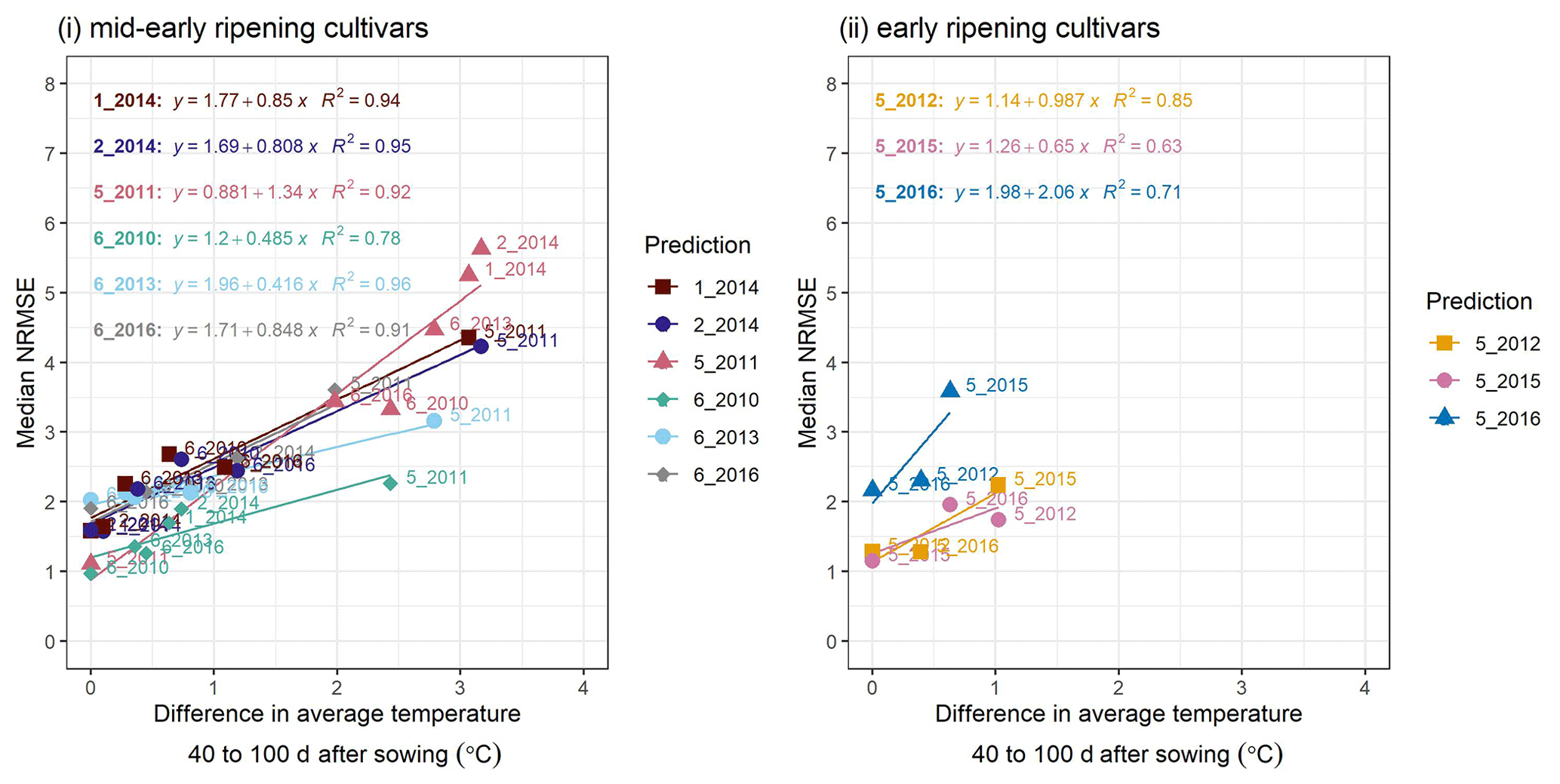
Figure C2 A cross-plot between the performance metric median NRMSE and the absolute difference in temperature between the site-year used for calibration and the prediction-target site-year, averaged over 40–100 d after sowing, for (i) mid-early and (ii) early ripening cultivars. Colours of the best-fit lines and points indicate the prediction-target site-year. Median NRMSE points at 0 ^∘C on the x-axis are calibration performance metrics for the target site-year while the remaining are prediction performance metrics. Point labels indicate the site-years to which the model was calibrated. The SPASS model was calibrated to observed phenological development (BBCH).

The mid-early cultivar at 5_2011 was poorly predicted by all mid-early cultivars, but was better predicted by early cultivars. Site-years 1_2014 and 2_2014 in Kraichgau, where the mid-early cultivar Grosso was grown, were the best predictors of each other. However, even though the early cultivar LG 30.217 was grown at 5_2015 and 5_2016, these two site-years were not the best predictors of each other. Similarly, site-years 2_2012 and 3_2011, where the late cultivar Canavaro was grown, were also not the best predictors of each other. In predictions for mid-early cultivars, a spread in median NRMSE ratio was seen when the model was calibrated to other mid-early cultivars. The mid-early cultivar at 1_2014 and 2_2014 in Kraichgau had a comparable prediction quality when the model was calibrated to the late cultivar grown in Kraichgau or to the mid-early cultivars grown on the Swabian Alb.

To explain the spread in prediction NRMSE within ripening groups, we examined the relationship between NRMSE and the difference in average temperature between the site-year used for calibration and the predicted or target site-year. The temperature was averaged over an interval of 40–100 d after sowing (i.e. approximate vegetative phase of development). For the mid-early ripening cultivars (Fig. C2i), the median NRMSE shows a clear correlation. Albeit tested with a limited number of site-years, early-ripening cultivars (Fig. C2ii) show a similar trend.

Appendix D: Platykurtic prior

An example of a platykurtic probability density function which is used as a weakly informative prior for the model parameters is shown in Fig. D1. It is a convolution of a uniform and normal distribution. The default, minimum, maximum, and standard deviation values from Table 2 were used in Eq. (10) to obtain the prior probability distribution for the estimated parameters.

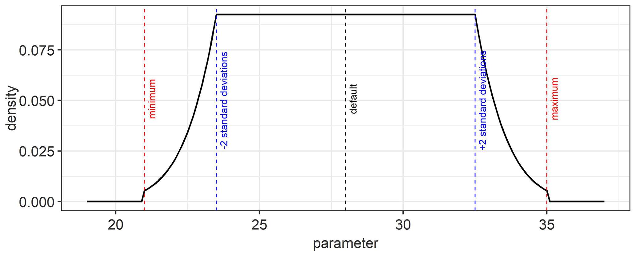
Figure D1 An example of the platykurtic probability density function that was used as a prior for the model parameters. The default, minimum, maximum, and standard deviation values for the parameter are used to define this function.