the Creative Commons Attribution 4.0 License.
the Creative Commons Attribution 4.0 License.
 | 11 May 2022
Global modelling of soil carbonyl sulfide exchanges
Camille Abadie
Fabienne Maignan
Marine Remaud
Jérôme Ogée
J. Elliott Campbell
Mary E. Whelan
Florian Kitz
Felix M. Spielmann
Georg Wohlfahrt
Richard Wehr
Nina Raoult
Ulli Seibt
Didier Hauglustaine
Sinikka T. Lennartz
Sauveur Belviso
David Montagne
Philippe Peylin
Carbonyl sulfide (COS) is an atmospheric trace gas of interest for C cycle research because COS uptake by continental vegetation is strongly related to terrestrial gross primary productivity (GPP), the largest and most uncertain flux in atmospheric CO2 budgets. However, to use atmospheric COS as an additional tracer of GPP, an accurate quantification of COS exchange by soils is also needed. At present, the atmospheric COS budget is unbalanced globally, with total COS flux estimates from oxic and anoxic soils that vary between −409 and −89 GgS yr−1. This uncertainty hampers the use of atmospheric COS concentrations to constrain GPP estimates through atmospheric transport inversions. In this study we implemented a mechanistic soil COS model in the ORCHIDEE (Organising Carbon and Hydrology In Dynamic Ecosystems) land surface model to simulate COS fluxes in oxic and anoxic soils. Evaluation of the model against flux measurements at seven sites yields a mean root mean square deviation of 1.6 pmol m−2 s−1, instead of 2 pmol m−2 s−1 when using a previous empirical approach that links soil COS uptake to soil heterotrophic respiration. However, soil COS model evaluation is still limited by the scarcity of observation sites and long-term measurement periods, with all sites located in a latitudinal band between 39 and 62∘ N and no observations during wintertime in this study. The new model predicts that, globally and over the 2009–2016 period, oxic soils act as a net uptake of −126 GgS yr−1 and anoxic soils are a source of +96 GgS yr−1, leading to a global net soil sink of only −30 GgS yr−1, i.e. much smaller than previous estimates. The small magnitude of the soil fluxes suggests that the error in the COS budget is dominated by the much larger fluxes from plants, oceans, and industrial activities. The predicted spatial distribution of soil COS fluxes, with large emissions from oxic (up to 68.2 pmol COS m−2 s−1) and anoxic (up to 36.8 pmol COS m−2 s−1) soils in the tropics, especially in India and in the Sahel region, marginally improves the latitudinal gradient of atmospheric COS concentrations, after transport by the LMDZ (Laboratoire de Météorologie Dynamique) atmospheric transport model. The impact of different soil COS flux representations on the latitudinal gradient of the atmospheric COS concentrations is strongest in the Northern Hemisphere. We also implemented spatiotemporal variations in near-ground atmospheric COS concentrations in the modelling of biospheric COS fluxes, which helped reduce the imbalance of the atmospheric COS budget by lowering soil COS uptake by 10 % and plant COS uptake by 8 % globally (with a revised mean vegetation budget of −576 GgS yr−1 over 2009–2016). Sensitivity analyses highlighted the different parameters to which each soil COS flux model is the most responsive, selected in a parameter optimization framework. Having both vegetation and soil COS fluxes modelled within ORCHIDEE opens the way for using observed ecosystem COS fluxes and larger-scale atmospheric COS mixing ratios to improve the simulated GPP, through data assimilation techniques.
- Article
(3226 KB) - Full-text XML
-
Supplement
(624 KB) - BibTeX
- EndNote


Carbonyl sulfide (COS) has been proposed as a tracer for constraining the simulated gross primary productivity (GPP) in land surface models (LSMs) (Launois et al., 2015; Remaud et al., 2022; Campbell et al., 2008). COS is an atmospheric trace gas that is scavenged by plants at the leaf level through stomatal uptake and irreversibly hydrolysed in a reaction catalysed by the enzyme carbonic anhydrase (CA) (Protoschill-Krebs et al., 1996). This enzyme also interacts with CO2 inside leaves. COS and CO2 follow a similar pathway from the atmosphere to the leaf interior. However, while CO2 is also released during respiration, plants generally do not emit COS (Montzka et al., 2007; Sandoval-Soto et al., 2005; Wohlfahrt et al., 2012). To infer GPP at the regional scale using COS observations, modellers can use measurements of ecosystem COS fluxes directly or measurements of atmospheric COS concentrations combined with an atmospheric transport inversion model, provided all COS flux components are taken into account. In both cases, net soil COS flux estimates are needed, as well as a functional relationship between GPP and COS uptake by foliage.
One important limitation for using COS as a tracer for GPP is the uncertainty that remains on the COS budget components. Several atmospheric transport inversion studies have suggested that an unidentified COS source located over the tropics, of the order of 400–600 GgS yr−1, was needed to close the contemporary COS budget (Berry et al., 2013; Glatthor et al., 2015; Kuai et al., 2015; Ma et al., 2021; Remaud et al., 2022). It was recently estimated to account for 432 GgS yr−1 by Ma et al. (2021). The hypothesis of a strong tropical oceanic source has not been substantiated by in situ COS and CS2 measurements in sea waters (Lennartz et al., 2017, 2020, 2021), except by Davidson et al. (2021), that invoke an oceanic source of 600 ± 400 GgS yr−1 based on direct measurements of sulfur isotopes. Clearly, an accurate characterization of all flux components of the atmospheric COS budget is still needed. In particular, the contribution of soils to the COS budget is poorly constrained, and improved estimates of their contribution may therefore provide clues to the attribution of the missing source.
A distinction is usually made between oxic soils that mainly absorb COS and anoxic soils that emit COS (Whelan et al., 2018). Regarding COS uptake, COS diffuses into the soil, where it is hydrolysed by CA contained in soil microorganisms such as fungi and bacteria (Smith et al., 1999). It is to be noted that COS can also be consumed by other enzymes, like nitrogenase, CO dehydrogenase, or CS2 hydrolase (Smith and Ferry, 2000; Masaki et al., 2021), but these enzymes are less ubiquitous than CA. The rate of uptake varies with soil type, temperature, and soil moisture (Kesselmeier et al., 1999; van Diest and Kesselmeier, 2008; Whelan et al., 2016). With high temperature or radiation, soils were also found to emit COS through thermal or photo degradation processes (Kitz et al., 2017, 2020; Whelan and Rhew, 2015; Whelan et al., 2016, 2018). Although such COS emissions can be large in some conditions, they have usually not been considered in atmospheric COS budgets.
Using the empirical relationship between soil COS uptake and soil respiration by Yi et al. (2007), Berry et al. (2013) provided new global estimates of COS uptake by oxic soils. Launois et al. (2015) proposed another empirical model, linking oxic soil COS uptake to H2 deposition based on the correlation between these two processes observed at Gif-sur-Yvette (Belviso et al., 2013). Models with a physical representation of the involved processes are also available. Sun et al. (2015) proposed such a mechanistic model including COS diffusion and reactions within layered soil. Ogée et al. (2016) also developed a mechanistic model including both COS uptake and production, with steady-state analytical solutions in homogeneous soils. When including such models in an LSM, the challenge is to spatialize them, which requires new variables or parameters not readily available at the global scale but inferred from field or lab experiments.
In this study, our goal is to provide and evaluate new global estimates of net soil COS exchange. To this end, we did the following:
- i.
We implemented an empirical-based and a mechanistic-based soil COS model in the ORCHIDEE (Organising Carbon and Hydrology In Dynamic Ecosystems) LSM.
- ii.
We evaluated the soil COS models at seven sites against in situ flux measurements.
- iii.
We estimated soil contributions to the COS budget at the global scale.
- iv.
We transported all COS sources and sinks using an atmospheric model and evaluated the concentrations against measurements of the National Oceanic and Atmospheric Administration (NOAA) air sampling network.
2.1 Description of the models
2.1.1 The ORCHIDEE Land Surface Model
The ORCHIDEE Land Surface Model is developed at the Institut Pierre-Simon Laplace (IPSL). The model version used here is the one involved in the Coupled Model Intercomparison Project Phase 6 (CMIP6) (Boucher et al., 2020; Cheruy et al., 2020). ORCHIDEE computes the carbon, water, and energy balances over land surfaces. It can be run at the site level or at the global scale. Fast processes such as soil hydrology, photosynthesis, and respiration are computed at a half-hourly time step. Other processes such as carbon allocation, leaf phenology, and soil carbon turnover are evaluated at a daily time step. Plant species are classified into 14 plant functional types (PFTs), according to their structure (trees, grasslands, or croplands), bioclimatic range (boreal, temperate, or tropical), leaf phenology (broadleaf or evergreen), and photosynthetic pathway (C3 or C4). The vegetation distribution in each grid cell is prescribed using yearly varying PFT maps, derived from the ESA Climate Change Initiative (CCI) land cover products (Poulter et al., 2015).
Soil parameters such as soil porosity, wilting point, and field capacity are derived from a global map of soil textures based on the FAO–USDA (Food and Agriculture Organization of the United Nations–United States Department of Agriculture) texture classification with 12 texture classes (Reynolds et al., 2000). The different textures for the USDA classification are presented in Table S1 in the Supplement. To better represent the observed soil conditions at the different sites that will be used for evaluation in this study, we substituted the soil textures initially assigned in ORCHIDEE from the USDA texture global map with the field soil textures translated into USDA texture classes (Table S2). In a previous study of vegetation COS fluxes in ORCHIDEE, Maignan et al. (2021) used the global soil map based on the Zobler texture classification (Zobler, 1986), which is reduced to three different textures in ORCHIDEE. However, the USDA soil classification gives a finer description of the different soil textures than the Zobler soil classification, considering 12 soil textures instead of 3. The move from the coarse Zobler classes to the finer USDA classes is found to be more important to the mechanistic model than to the empirical model. Since the USDA texture classes are more accurate with its finer discretization of soil textures, in the rest of this study, we only illustrate the results based on the USDA texture classification.
For site level simulations, the ORCHIDEE LSM was forced by local micro-meteorological measurements obtained from the FLUXNET network at the FLUXNET sites following the Creative Commons (CC-BY 4.0) license (Pastorello et al., 2020) and at the remaining sites by other local meteorological measurements performed together with the COS fluxes measurements when available, eventually gap-filled using the 0.25∘ × 0.25∘ hourly reanalysis from the fifth generation of meteorological analyses of the European Centre for Medium-Range Weather Forecasts (ECMWF) (ERA5) (Hersbach et al., 2020). Global simulations were forced by the 0.5∘ and 6-hourly CRU JRA reanalysis (University of East Anglia Climatic Research Unit–Japanese Reanalysis; Friedlingstein et al., 2020). Near-surface COS concentrations (denoted Ca below) were prescribed using monthly mean atmospheric COS concentrations at the first vertical level of the LMDZ (Laboratoire de Météorologie Dynamique) atmospheric transport model (GCM, general circulation model; see description below in Sect. 2.1.3), forced with optimized COS surfaces fluxes. The latter have been inferred by atmospheric inverse modelling from the COS surface measurements of the NOAA network (Remaud et al., 2022). Simulations with constant atmospheric COS concentrations at a mean global value of 500 ppt were also run to evaluate the impact of spatiotemporal variations in near-surface COS concentrations versus a constant value. Near-surface CO2 concentrations were estimated using global yearly mean values provided by the TRENDY (Trends in the land carbon cycle) project (Sitch et al., 2015).
2.1.2 COS soil models
The empirical soil COS flux model
We implemented in the ORCHIDEE LSM the soil COS flux model from Berry et al. (2013), which assumes that COS uptake is proportional to CO2 production by soil respiration, following Yi et al. (2007). Although Yi et al. (2007) reported a relationship between soil COS uptake and total soil respiration, including root respiration, Berry et al. (2013) assumed that COS flux was proportional to soil heterotrophic respiration only. The rationale behind this assumption is that soil CA concentration is related to soil organic matter content and thus ecosystem productivity (Berry et al., 2013). As heterotrophic respiration is also linked to productivity, Berry et al. (2013) considered soil COS uptake to be proportional to soil heterotrophic respiration. However, soil respiration alone did not correlate well in incubation studies (Whelan et al., 2016). As the proportionality between COS fluxes and soil respiration has only been demonstrated for the total (heterotrophic and autotrophic) soil respiration (Yi et al., 2007), we used in this study total soil respiration as a scaling factor for soil COS uptake. This model will be referred to as the empirical model.
The influence of soil temperature and moisture are included in the calculation of soil respiration. Thus, we computed soil COS flux Fsoil, empirical (pmol COS m−2 s−1) as follows:
where Resptot is total soil respiration (µmol CO2 m−2 s−1) and ksoil is a constant equal to 1.2 pmol COS per µmol CO2 that converts CO2 production from respiration to COS uptake. The value of 1.2 pmol COS per µmol CO2 was estimated from field chamber measurements in a pine and broadleaf mixed forest (Dinghushan Biosphere Reserve, southern China) from Yi et al. (2007). In ORCHIDEE, we calculated the total soil respiration as the sum of soil heterotrophic respiration within the soil column, including that of the litter, and root autotrophic respiration.
The mechanistic soil COS flux model
The mechanistic COS soil model of Ogée et al. (2016) describes both soil COS uptake and production. This model includes COS diffusion in the soil matrix, COS dissolution, and hydrolysis in the water-filled pore space and COS production under low redox conditions. The soil is assumed to be horizontally homogeneous so that the soil COS concentration C (mol m−3) is only a function of time t (s) and soil depth z (m). The mass balance equation for COS can then be written as (Ogée et al., 2016)
where εtot is the soil total porosity (m3 air per cubic metre soil), Fdiff is the diffusional flux of COS (mol m−2 s−1), S is the COS consumption rate (mol m−3 s−1), and P the COS production rate under low redox conditions (mol m−3 s−1).
Under steady-state conditions and uniform soil temperature, moisture, and porosity profiles, an analytical solution of Eq. (2) can be found (Ogée et al., 2016). We assume that the environmental conditions, such as soil temperature and moisture, are constant in ORCHIDEE over the 30 min model time step. We also assume chemical equilibrium between the gaseous and the dissolved COS, neglecting advection as suggested by Ogée et al. (2016). In these conditions, the typical timescale for COS diffusion in the upper active soil layer is much shorter than the 30 min model time step. Although Eq. (2) could also be solved numerically using the soil discretization in ORCHIDEE, we preferred to use the analytical solution, using the mean soil moisture and temperature averaged over the first few soil layers (down to about 9 cm deep), weighted by the thickness of each soil layer. Assuming fully mixed atmospheric conditions within and below the vegetated canopy, we also assumed that the COS concentration at the soil surface C(z=0) is equal to the near-surface COS concentration Ca. With these boundaries' conditions, the steady-state COS flux at the soil surface Fsoil, mechanistic (mol m−2 s−1) is (Ogée et al., 2016)
where k is the first-order COS consumption rate constant within the soil
(s−1), B is the solubility of COS in water (m3 water per cubic metre air),
θ is the soil volumetric water content (m3 water per cubic metre soil),
D is the total effective COS diffusivity (m2 s−1), (m), and zmax is the soil depth below which the COS
production rate and the soil COS gradient are assumed negligible (Ogée
et al., 2016). In the following, zmax is set at 0.09 m.
COS diffusion
The total effective COS diffusivity in soil D includes the effective
diffusivity of gaseous COS Deff,a (m3 air per metre soil per second) and dissolved COS Deff,l (m3 water per metre soil per second) through the soil matrix:
The solubility of COS in water B is calculated using Henry's law constant KH (mol m−3 Pa−1):
where R=8314 J mol−1 K−1 is the ideal gas constant, T is the soil temperature (K), and (Wilhelm et al., 1977)
The effective diffusivity of gaseous COS Deff,a is expressed as (Ogée et al., 2016)
where D0,a is the binary diffusivity of COS in the air (m2 air s−1), τa is the air tortuosity factor representing the tortuosity of the air-filled pores, and εa is the air-filled porosity (m3 air per cubic metre soil). The binary diffusivity of COS in the air D0,a is expressed following the Chapman–Enskog theory for ideal gases (Bird et al., 2002) and depends on temperature and pressure:
where m2 s−1 (Massman, 1998).
The expression of the air tortuosity factor τa depends on whether the soil is repacked or undisturbed. In ORCHIDEE, repacked soils correspond to the agricultural soils represented by the C3 and C4 crops. Soils not covered by crops are considered undisturbed soils. The expression of τa for repacked soils τa,r is given by Moldrup et al. (2003):
where φ is the soil porosity (m3 m−3) that includes the air-filled and water-filled pores. Soil porosity is assumed constant through the soil column in ORCHIDEE and is determined by the USDA texture global map. The air-filled porosity εa is calculated as .
The expression of τa for undisturbed soils τa,u is given in Deepagoda et al. (2011). We chose this expression rather than the expression proposed by Moldrup et al. (2003) for undisturbed soils because it appears to be more accurate and does not require information on the pore-size distribution (Ogée et al., 2016):
In a similar way to COS diffusion in the gas phase, the effective diffusivity of dissolved COS Deff,l is described by Ogée et al. (2016):
where D0,l is the binary diffusivity of COS in the free water (m2 water s−1) and τl is the tortuosity factor for solute diffusion. The binary diffusivity of COS in the free water D0,l is described using an empirical formulation proposed by Zeebe (2011) for CO2, which only depends on temperature:
where T0=216 K (Ogée et al., 2016) and m2 s−1 (Ulshöfer et al., 1996).
The expression of τl is the same for repacked and undisturbed soils. We used the expression given by Millington and Quirk (1961) as a good compromise between simplicity and accuracy (Moldrup et al., 2003):
COS consumption
COS can be destroyed by biotic and abiotic processes. The abiotic process
corresponds to COS hydrolysis in soil water at an uncatalysed rate kuncat (s−1), which depends on soil temperature T (K) and pH
(Elliott et al., 1989):
where pKw is the dissociation constant of water.
This uncatalysed hydrolysis is quite low compared to the COS hydrolysis catalysed by soil microorganisms, which is the main contribution of COS uptake by soils (Kesselmeier et al., 1999; Sauze et al., 2017; Meredith et al., 2018). The enzymatic reaction catalysed by CA follows Michaelis–Menten kinetics. The turnover rate kcat (s−1) and the Michaelis–Menten constant Km (mol m−3) of this reaction depend on temperature. The temperature dependence of the ratio is expressed as (Ogée et al., 2016)
where ΔHa, ΔHd, and ΔSd are thermodynamic parameters, such as ΔHa=40 kJ mol−1, ΔHd=200 kJ mol−1, and ΔSd=660 J mol−1 K−1.
The total COS consumption rate by soil k (s−1) is described with respect to the uncatalysed rate at T=298.15 K and pH=4.5 (Ogée et al., 2016):
where fCA is the CA enhancement factor, which characterizes the soil
microbial community that can consume COS. The CA enhancement factor depends
on soil CA concentration, temperature, and pH. Ogée et al. (2016)
reported that its values range between 21 600 and 336 000, with a median
value at 66 000. We adapted the values of fCA found in Meredith et
al. (2019) to have a CA enhancement factor that depends on ORCHIDEE biomes
(Table A1 in Appendix A).
Oxic soil COS production
Abiotic oxic soil COS production has been observed at high soil temperature
(Maseyk et al., 2014; Whelan and Rhew, 2015; Kitz et al., 2017, 2020;
Spielmann et al., 2019a, 2020). However, photodegradation has also been
proposed as an abiotic production mechanism in oxic soils (Whelan and Rhew,
2015; Kitz et al., 2017, 2020). Abiotic COS production is still not well
understood but was assumed to originate from biotic precursors (Meredith et
al., 2018).
In Ogée et al. (2016), the production rate P is described as independent of soil pH but depends on soil temperature and redox potential. This dependence on soil redox potential enables us to consider the transition between oxic and anoxic soils. However, because little information is available on soil redox potential at the global scale, its influence cannot yet be represented in a spatially and temporally dynamic way in a land surface model such as ORCHIDEE. Thus, we decided to use the production rate described in Whelan et al. (2016) that only depends on soil temperature and land use type:
where Poxic is expressed in pmol g−1 min−1, T is soil
temperature (∘C), and α and β are parameters
determined by Whelan et al. (2016) for each land use type using the
least-squares fitting approach. We adapted the values of α and
β given for four land use types to ORCHIDEE biomes (Table A2 in Appendix A). Values of α and β for deserts could not be estimated by
Whelan et al. (2016) because COS emission for this biome was not found to
increase with temperature. Figure 11 in Whelan et al. (2016) shows that COS
emission from a desert soil is always near zero for temperatures ranging
from 10 to 40 ∘C. Moreover, COS emission from a
desert soil is also found to be near zero in Fig. 1 of Meredith et al. (2018). This could be explained by a lack of organic precursors to produce
COS (Whelan et al., 2016). Therefore, we considered that desert soils, which
correspond to a specific non-vegetated PFT in ORCHIDEE, do not emit COS. For
other ORCHIDEE biomes, COS production was estimated using α and
β for each PFT and the mean soil temperature over the top 9 cm. The
unit of Poxic was converted from pmol g−1 min−1 to mol m−3 s−1 (in Eq. 3) using soil bulk density information from
the Harmonized World Soil Database (HWSD; FAO/IIASA/ISRIC/ISSCAS/JRC, 2012).
Anoxic soil COS emission
Several studies have shown direct COS emissions by anoxic soils (Devai and
DeLaune, 1997; de Mello and Hines, 1994; Whelan et al., 2013; Yi et al.,
2007). This has been linked to a strong activity of sulfate reduction
metabolisms in highly reduced environments such as wetlands (Aneja et al.,
1981; Kanda et al., 1992; Whelan et al., 2013; Yi et al., 2007). A previous
approach developed by Launois et al. (2015) was based on the representation
of seasonal methane emissions by Wania et al. (2010) in the LPJ–WHyME (Lund–Potsdam–Jena–Wetland Hydrology and Methane) model
to represent anoxic soils in ORCHIDEE. The mean values of soil COS emissions
from Whelan et al. (2013) were used to attribute to each grid point a value
of soil COS emission. In this approach by Launois et al. (2015), salt
marshes were not represented despite their strong COS emissions found in
Whelan et al. (2013). Emissions from rice paddies were also neglected. Thus,
COS emissions from anoxic soils peaked in summer over the high latitudes,
following methane production.
Because of the scarce knowledge on anoxic soil COS exchange, here we propose another approach to represent the contribution of anoxic soils, which could be compared to the previous approach developed by Launois et al. (2015). To represent the distribution of anoxic soils, we selected the regularly flooded wetlands from the map developed by Tootchi et al. (2019), as represented in Fig. 1. The regularly flooded wetlands cover 9.7 % of the global land area, which is among the average values found in the literature ranging from 3 % to 21 % (Tootchi et al., 2019). Then, in ORCHIDEE each pixel is considered either anoxic following the wetland map distribution from Tootchi et al. (2019) or oxic for the rest of the land surfaces. The pixels defined as anoxic soils are considered flooded through the entire year: the seasonal variations of the flooding, as happen during the monsoon seasons, are consequently neglected.
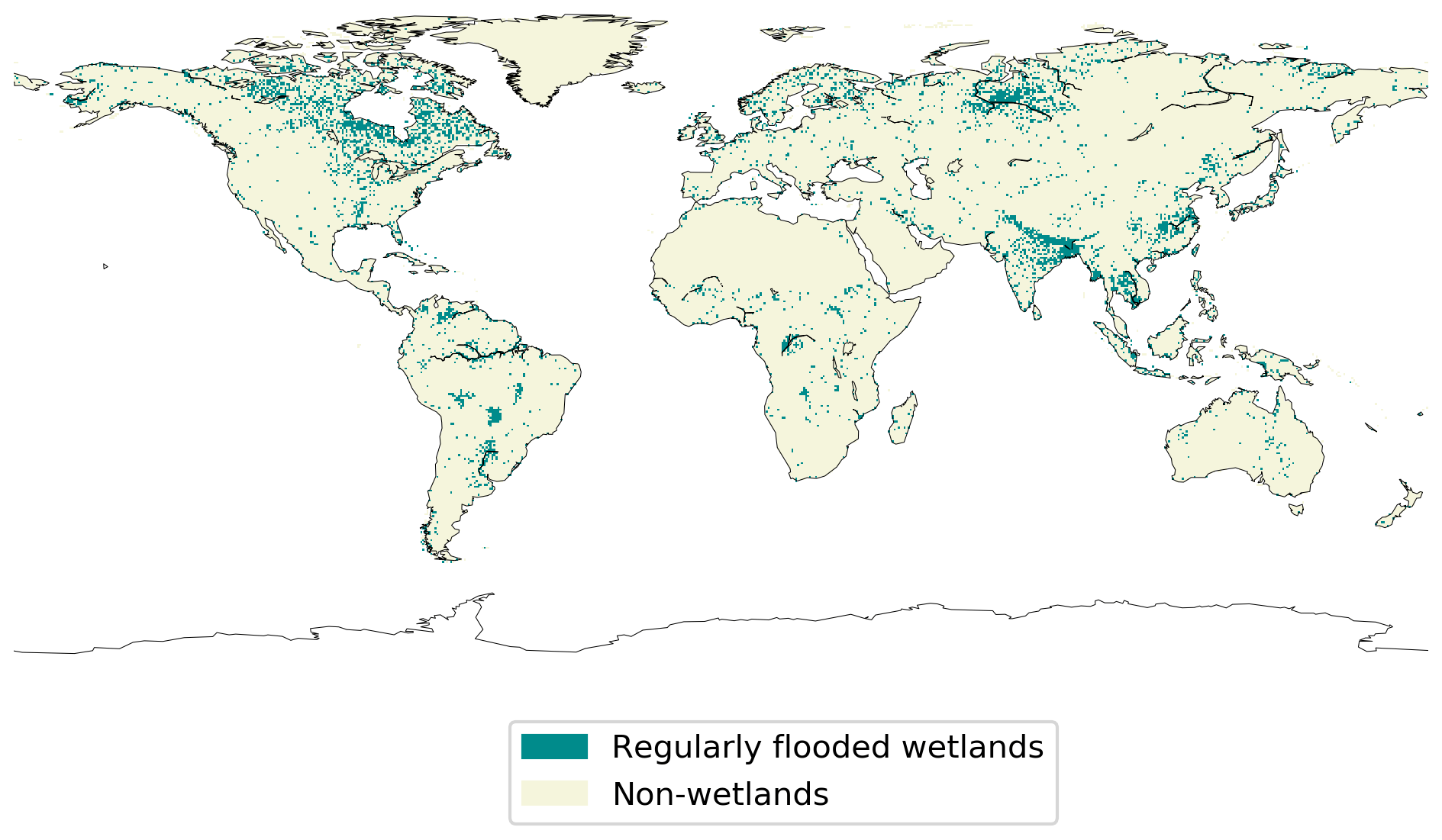
Figure 1Map of wetlands distribution used to represent anoxic soils in ORCHIDEE. The map resolution is 0.5∘ × 0.5∘ (adapted from Tootchi et al., 2019).
On anoxic pixels, we represent anoxic soil COS flux with a production rate based on the expression developed by Ogée et al. (2016):
where Pref (mol m−2 s−2) is the reference production term, Tref is a reference soil temperature (K), and Q10 is the multiplicative factor of the production rate for a 10 ∘C increase in soil temperature (unitless). As anoxic soil production ranges from 10 to 300 pmol m2 s−1 for salt marshes and is usually below 10 pmol m−2 s−1 for freshwater wetlands (Whelan et al., 2018), the reference production term was set to 10 pmol m−2 s−1.
All the variables and constants of the empirical and mechanistic models are presented in Tables A3 and A4 in Appendix A.
2.1.3 The atmospheric chemistry transport model LMDZ
To simulate the COS atmospheric distribution, we use an “offline” version of the Laboratoire de Météorologie Dynamique general circulation model (GCM), LMDZ 6 (Hourdin et al., 2020), which has been used as the atmospheric component in the IPSL coupled model for CMIP6. The LMDZ GCM has a spatial resolution of 3.75∘ long. × 1.9∘ lat. with 39 sigma-pressure layers extending from the surface to about 75 km, corresponding to a vertical resolution of about 200–300 m in the planetary boundary layer, and a first level at 33 m above sea or ground level. The model u and v wind components were nudged towards winds from the ERA5 reanalysis with a relaxation time of 2.5 h to ensure realistic wind advection (Hourdin and Issartel, 2000; Hauglustaine et al., 2004). The ECMWF fields are provided every 6 h and interpolated onto the LMDZ grid. This version has been shown to reasonably represent the transport of passive tracers (Remaud et al., 2018). The offline model uses pre-computed mass fluxes provided by this full LMDZ GCM version and only solves the continuity equation for the tracers, which significantly reduces the computation time. In the following, we refer to this offline version as LMDZ. The model time step is 30 min, and the output concentrations are 3-hourly averages.
The atmospheric COS oxidation is computed from pre-calculated OH monthly concentration fields produced from a simulation of the INCA (Interaction with Chemistry and Aerosols) model (Folberth et al., 2006; Hauglustaine et al., 2004, 2014) coupled to LMDZ. The atmospheric OH oxidation of COS amounts to 100 GgS yr−1 in the model. Similarly, the COS photolysis rates are also pre-calculated with the INCA model, which uses the Troposphere Ultraviolet and Visible (TUV) radiation model adapted for the stratosphere (Terrenoire et al., 2022). The temperature-dependent carbonyl sulfide absorption cross-sections from 186.1 to 296.3 nm are taken from Burkholder et al. (2019). The calculated photolysis rates are averaged over the period 2008–2018 and prescribed to LMDZ. Implemented in LMDZ, the COS photolysis in the stratosphere amounts to about 30 GgS yr−1, which is of the same order of magnitude as previous estimates: 21 GgS yr−1 (71 % of 30 GgS yr−1) by Chin and Davis (1995), between 11 and 21 GgS yr−1 by Kettle et al. (2002), and between 16 and 40 GgS yr−1 by Ma et al. (2021).
2.2 Observation data sets
2.2.1 Description of the sites
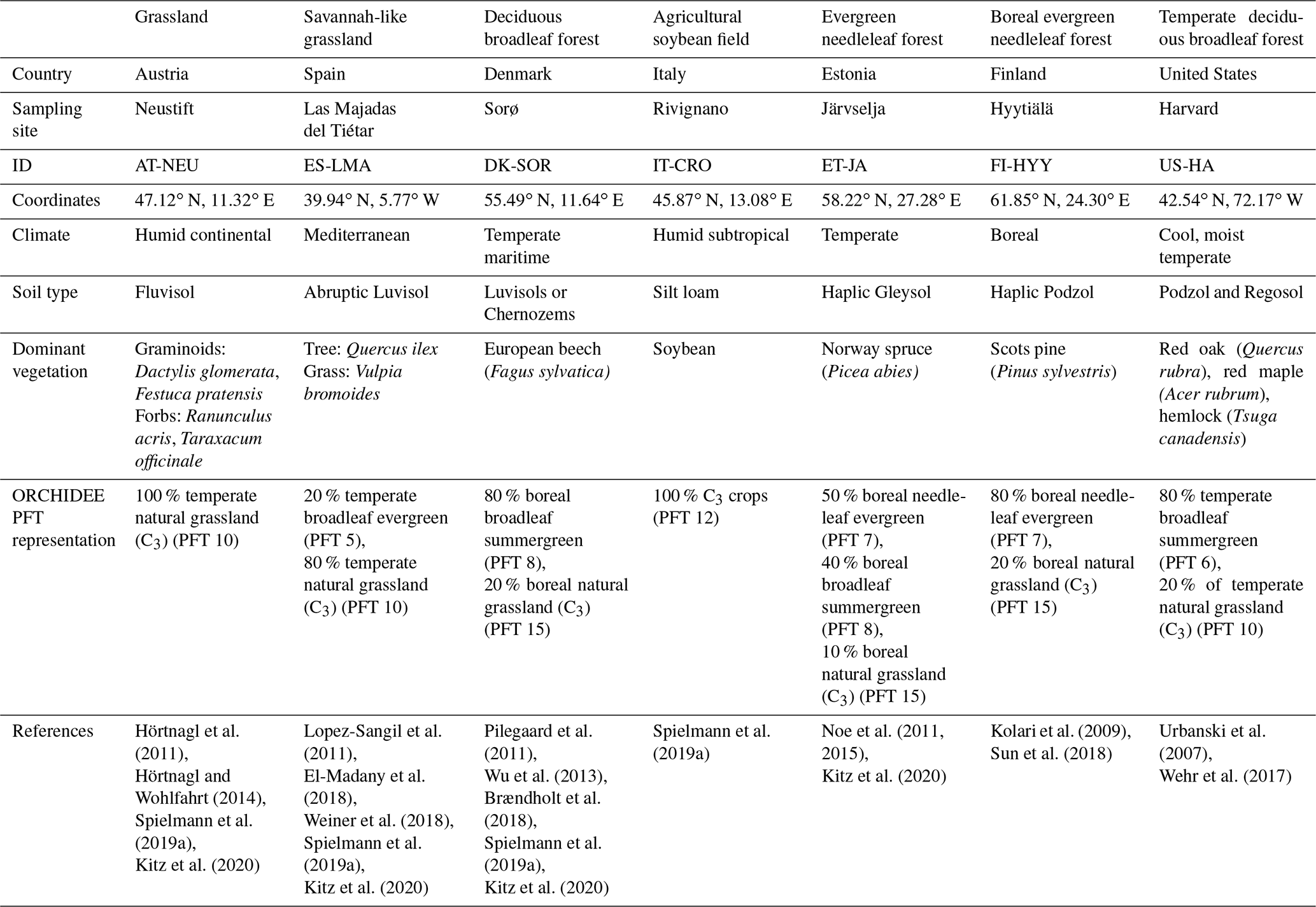
The description of the studied sites is given in Table 1.
Table 1Lists the sites' characteristics including their identification name, location, climate, soil type, dominant vegetation and species, corresponding PFT fractions we used for the ORCHIDEE simulations, and reference studies for more details. The spatial distribution of the sites is represented in Fig. B1 in Appendix B.
2.2.2 Soil COS flux determination at selected sites
Soil COS flux chamber measurements were conducted in 2015 at AT-NEU; in 2016 at DK-SOR, ES-LMA, and ET-JA; and in 2017 at IT-CRO (abbreviations as in Table 1). The aboveground vegetation was removed 1 d before the measurements if needed, and the fluxes were derived from concentration measurements using a quantum cascade laser (see Kitz et al., 2020, and Spielmann et al., 2020, 2019a). At AT-NEU, DK-SOR, ES-LMA, and IT-CRO, a random forest model was calibrated against the manual chamber measurements and then used to simulate half-hourly soil COS fluxes in Spielmann et al. (2019a). We compared the ORCHIDEE half-hourly simulated fluxes to half-hourly outputs of the random forest model. This enabled studying the diel cycle and computing daily observations with no sampling bias for the study of the seasonal cycle. Soil COS fluxes for ET-JA were derived by using the same training method as the one used in Spielmann et al. (2019a).
At FI-HYY, soil COS fluxes were measured using two automated soil chambers in 2015. These chambers were connected to a quantum cascade laser spectrometer to calculate soil COS fluxes from concentration measurements (see Sun et al., 2018, for more information on the experimental setup). Any vegetation was removed from the chambers before the measurements.
At US-HA, soil COS fluxes in 2012 and 2013 were not directly measured but derived from flux-profile measurements, connected to CO2 soil chamber measurements and profiles. A sub-canopy flux gradient approach was used to partition canopy uptake from soil COS fluxes. For more information on this approach and its limitations, see Wehr et al. (2017).
In the study of soil COS fluxes, the difficulty of performing soil COS flux measurements must be acknowledged, as well as the differences between experimental setups and methods to retrieve soil COS fluxes. These limitations are illustrated in the set of observations selected here. Aboveground vegetation had to be removed at some sites to not measure the plant contribution in addition to soil COS fluxes (Sun et al., 2018; Spielmann et al., 2019a; Kitz et al., 2020). Vegetation removal prior to the measurements might lead to artefacts in the observations. Some components of the measuring system can also emit COS. In this case, a blank system is needed to apply a post-correction to the measured fluxes (Sun et al., 2018; Kitz et al., 2020). Litter was left in place at the measurement sites.
2.2.3 COS concentrations at the NOAA Earth System Research Laboratories (ESRL) sites
The NOAA surface flask network provides long-term measurements of the COS mole fraction at 14 locations at weekly to monthly frequencies from the year 2000 onwards. We use an extension of the data initially published in Montzka et al. (2007). The data were collected as paired flasks analysed using gas chromatography and mass spectrometry. The stations located in the Northern Hemisphere had sample air masses coming from the entire Northern Hemisphere domain above 30∘. Among them, the sites LEF, NWR, HFM, and WIS have mostly continental footprints (Remaud et al., 2022), while the sites SPO, CGO, and PSA sample mainly oceanic air masses of the Southern Hemisphere (Montzka et al., 2007). The locations of these sites are depicted in Fig. B1 in Appendix B.
2.3 Simulations
2.3.1 Spin-up phase
A “spin-up” phase was performed before each simulation, which enabled all carbon pools to stabilize and the net biome production to oscillate around zero. Reaching the equilibrium state is accelerated in the ORCHIDEE LSM thanks to a pseudo-analytical iterative estimation of the carbon pools, as described in Lardy et al. (2011). For site simulations, the spin-up was performed by cycling the years available in the forcing files of each site, for a total of about 340 years. For global simulations, the spin-up phase of 340 years was performed by cycling over 10 years of meteorological forcing files in the absence of any disturbances.
2.3.2 Transient phase
Following the spin-up phase we ran a transient simulation of about 40 years that introduced disturbances such as climate change, land use change, and increasing CO2 atmospheric concentrations.
This transient phase was performed by cycling over the available years for site simulations. For global simulations, the transient phase was run where we introduced disturbances from 1860 to 1900. After this transient phase, COS fluxes were simulated from 1901 to 2019.
2.3.3 Atmospheric simulations: sampling and data processing
We ran the LMDZ6 version of the atmospheric transport model described above for the years 2009 to 2016. We started from a uniform initial condition, and we removed the first year, as it is considered to be part of the spin-up period. The COS fluxes used as model inputs are presented in Table 2. The fluxes are given as a lower boundary condition, called the surface, of the atmospheric transport model (LMDZ), which then simulates the transport of COS by large-scale advection and sub-grid scale processes such as convection and boundary layer turbulence. In this study, we only evaluate the sensitivity of the latitudinal gradient and seasonal cycle of COS concentrations to the soil COS fluxes. The horizontal gradient aims at validating the latitudinal repartition of the surface fluxes, while the seasonal cycle partly reflects the seasonal exchange with the terrestrial sink, which peaks in spring/summer. This study does not aim at reproducing the mean value, as the top-down COS budget is currently unbalanced, with a source component missing (Whelan et al., 2018; Remaud et al., 2022; see Table 3).
Table 2Sink and source components of COS budget used in this study. Mean magnitudes and standard deviations of different types of fluxes are given for the period 2009–2016.
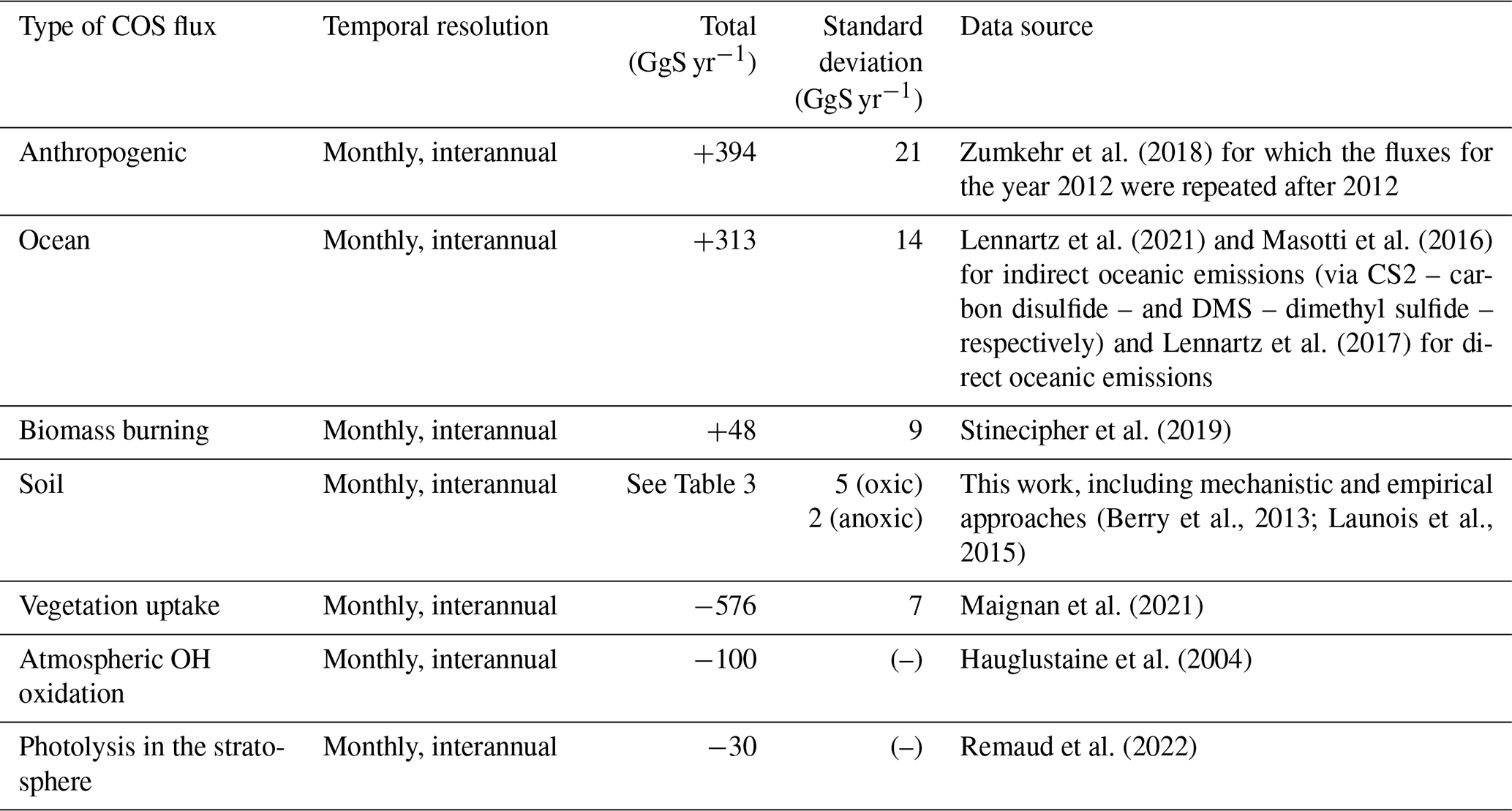
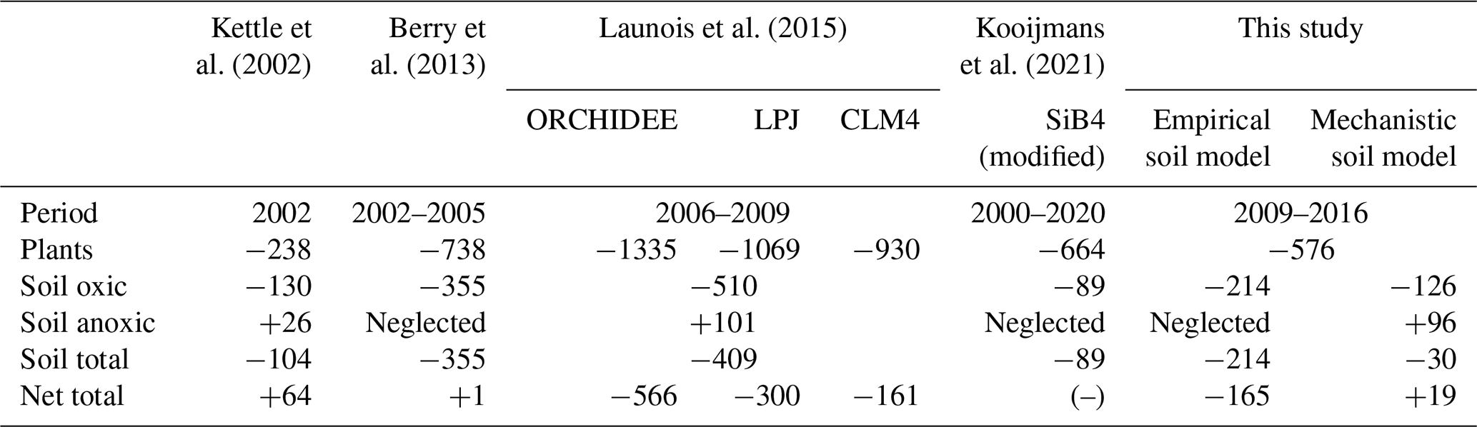
Table 3Comparison of soil COS budget per year (GgS yr−1). The net total COS budget is computed by adding all sources and sinks of COS (anthropogenic, ocean, biomass burning, soils, vegetation, atmospheric OH oxidation, and photolysis in the atmosphere) used to transport COS fluxes (Table 2). CLM: Community Land Model. SiB: Simple Biosphere Model.
For each COS observation, the 3D simulated concentration fields were sampled at the nearest grid point to the station and at the closest hour of the measurements. For each station, the curve fitting procedure developed by the NOAA Climate Monitoring and Diagnostic Laboratory (NOAA CMDL) (Thoning et al., 1989) was applied to modelled and observed COS time series to extract a smooth detrended seasonal cycle. We first fitted a function including a first-order polynomial term for the growth rate and two harmonic terms for seasonal variations. The residuals (raw time series minus the smooth curve) were fitted using a low-pass filter with either 80 or 667 d as short-term and long-term cut-off values. The detrended seasonal cycle is defined as the smooth curve (full function plus short-term residuals) minus the trend curve (polynomial plus long-term residuals). Regarding vegetation COS fluxes (Maignan et al., 2021), we added the possibility of using spatially and temporally varying atmospheric COS concentrations, as for soil.
2.4 Numerical methods for model evaluation and parameter optimization
2.4.1 Statistical scores
We evaluated modelled soil COS fluxes against field measurements using the root mean square deviation (RMSD) as
where N is the number of considered observations, is the nth observed COS flux, and is the nth modelled COS flux, and the relative RMSD (rRMSD) as
which is the RMSD divided by the mean value of observations.
Simulated atmospheric COS concentrations were evaluated by computing the normalized standard deviation (NSD), which is the standard deviation of the simulated concentrations divided by the mean of the observed concentrations, and the Pearson correlation coefficients (r) between simulated and observed COS concentrations. The closer NSD and r values are to 1, the better the model accuracy is.
2.4.2 Data assimilation
One of the main difficulties with the implementation of a model is to define the parameter values that lead to the most accurate representation of the processes in ORCHIDEE. Calibrating the model parameters is of interest as Ogée et al. (2016) indicate that some of the model parameters such as fCA and the production term parameters have to be constrained by observations. Moreover, the default values for the soil COS model parameters used in this study (Tables A1 and A2 in Appendix A) are determined by laboratory experiments (Ogée et al., 2016; Whelan et al., 2016), which is why it is interesting to study how the values obtained by calibration against field observations differ from these default values. Data assimilation (DA) aims at producing an optimal estimate by combining observations and model outputs. In this study, we used DA to find the model parameter values that improve the fit between simulated and observed soil COS fluxes from the empirical and the mechanistic models. We used the ORCHIDEE Data Assimilation System (ORCHIDAS), which is based on a Bayesian framework. ORCHIDAS has been described in detail in previous studies (Bastrikov et al., 2018; Kuppel et al., 2014; MacBean et al., 2018; Peylin et al., 2016; Raoult et al., 2021), so below we only briefly present the method. Assuming that the observations and model outputs follow a Gaussian distribution, we aim at minimizing the following cost function J(x) by optimizing the model parameters (Tarantola, 2005):
where x is the vector of parameters to optimize and y is the observations. The first part of the cost function measures the mismatch between the observations and the model, and the second part represents the mismatch between the prior parameter values xb and the considered set of parameters x. Both terms of the cost function are weighted by the prior covariance matrices for the observation errors E−1 and parameter errors B−1. The minimization of the cost function follows the genetic algorithm (GA) method, which is derived from the principles of genetics and natural selection (Goldberg, 1989; Haupt and Haupt, 2004) and is described for ORCHIDAS in Bastrikov et al. (2018).
For each soil COS model, we selected the eight most important parameters to which soil COS fluxes are sensitive following sensitivity analyses (Sect. 2.4.3). The observation sites selected for sensitivity analyses and DA are the ones with the largest number of observations for model parameter calibration, which are FI-HYY and US-HA.
2.4.3 Sensitivity analyses
We conducted sensitivity analyses at two contrasting sites (FI-HYY and US-HA) to determine which model parameters have the most influence on the simulated soil COS fluxes from the empirical and the mechanistic models. Sensitivity analyses can help to identify the key parameters before aiming at calibrating these parameters. Indeed, focusing on the key model parameters for calibration limits both the computational cost of optimization that increases with the number of parameters and the risk of overfitting.
The Morris method (Morris, 1991; Campolongo et al., 2007) was used for the sensitivity analysis, as it is relatively time efficient and enables ranking the parameters by importance. This qualitative method requires only a small number of simulations, (p+1)n, where p is the number of parameters and n is the number of random trajectories generated (here, n=10).
We selected a set of parameters for the Morris sensitivity analyses based on previous sensitivity analyses conducted on soil parameters in ORCHIDEE (Dantec-Nédélec et al., 2017; Raoult et al., 2021; Mahmud et al., 2021). A distinction is made between the soil COS model parameters called first-order parameters (fCA, α, and β for the mechanistic model and ksoil for the empirical model) and parameters called second-order parameters related to soil hydrology, carbon uptake and allocation, phenology, conductance, or photosynthesis (18 parameters; see Tables S3 and S4). The range of variation in the second-order parameters is described in previous studies using ORCHIDEE (Dantec-Nédélec et al., 2017; Raoult et al., 2021; Mahmud et al., 2021). For the first-order parameters, the range of variation is described in Yi et al. (2007) for ksoil (±1.08 pmol COS per µmol CO2) and in Table 1 in Meredith et al. (2019) for fCA. The ranges of variation for α and β parameters are not directly given in the literature and were calculated based on information from the production parameters defined in Meredith et al. (2018) (Text S1 and Table S5).
3.1 Site-scale COS fluxes
3.1.1 Soil COS flux seasonal cycles
Figure 2 shows the seasonal cycles of soil COS fluxes at the different sites where measurements were conducted. The empirical model mainly differs from the mechanistic model with a stronger seasonal amplitude of soil COS fluxes (34 % higher), except at the sites where a net COS production is found with the mechanistic model in summer (ES-LMA and IT-CRO). At all sites, the empirical model shows that the simulated uptake increases in spring, reaching a maximum in summer, and decreases in autumn with a minimal uptake during winter. The strong COS uptake in summer from the empirical model can be explained by the proportionality of soil COS uptake to simulated soil respiration, which increases with the high temperatures in summer. In contrast, the mechanistic model depicts almost no seasonality at all the sites where no net COS production is found over the year. As the mechanistic model represents both soil COS uptake and production, the increase in COS production due to higher temperature in summer compensates part of the COS uptake (Fig. C1 in Appendix C). While the uptake from the empirical model is often higher than the one computed with the mechanistic model in summer, soil COS uptake in winter is stronger with the mechanistic representation.
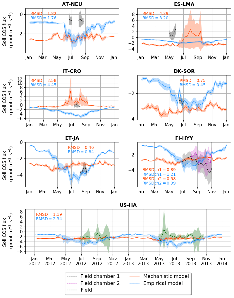
Figure 2Seasonal cycle of weekly average net soil COS fluxes (pmol m−2 s−1) at AT-NEU, ES-LMA, IT-CRO, DK-SOR, ET-JA, FI-HYY, and US-HA. The shaded areas around the observation and simulation curves represent the standard deviation over a week for each site. Soil COS fluxes are computed with a variable atmospheric COS concentration. RMSD values between the simulated and observed fluxes are given with the respective model colour at each site and for both soil chambers at FI-HYY (ch1 and ch2).
The scarcity of field measurements at AT-NEU, ES-LMA, IT-CRO, DK-SOR, and ET-JA does not allow for an evaluation of the simulated seasonality of COS fluxes. However, at US-HA, the absence of seasonality from May to October in the observations is also found in the mechanistic model, while a maximum net soil COS uptake is reached with the empirical model.
We found that the mechanistic model is in better agreement with the observations for four (IT-CRO, ET-JA, FI-HYY, and US-HA) out of the seven sites, with a mean of 1.58 pmol m−2 s−1 and 2.03 m−2 s−1 for the mechanistic and empirical model, respectively. However, the mechanistic model struggles to reproduce soil COS fluxes at AT-NEU and ES-LMA, with an overestimation of soil COS uptake or an underestimation of soil COS production at AT-NEU and a delay in the simulated net COS production at ES-LMA. We might suspect that the removal of vegetation at these sites prior to the measurements could have artificially enhanced COS production in the observations. Indeed, the removal of vegetation could change soil structure and increase the availability of soil organic matter to degradation (Whelan et al., 2016). AT-NEU and ES-LMA are grassland sites for which soils are expected to receive higher light intensity than forest soils. These sites also show a high mean soil temperature of about 20 ∘C during the measurement periods. Therefore, high soil temperature and light intensity on soil surface could have enhanced soil COS production, as it was related to thermal or photo degradation of soil organic matter (Kitz et al., 2017, 2020; Whelan and Rhew, 2015; Whelan et al., 2016, 2018). This is not the case at FI-HYY, ET-JA, or DK-SOR, where soil temperature is much lower (mean value about 10 ∘C at FI-HYY and 15 ∘C at ET-JA and DK-SOR during the measurement periods) and the forested cover decreases the radiation level reaching the soil. Note that herbaceous biomass is also likely to be higher in grasslands than in forests. Besides, AT-NEU and ES-LMA are managed grassland sites with nitrogen inputs. Then, soil COS production could also be enhanced by a high nitrogen content as suggested by several studies (Kaisermann et al., 2018; Kitz et al., 2020; Spielmann et al., 2020), which is not represented in our models. The mechanistic model is able to represent a net COS production at IT-CRO but overestimates it. This might highlight the importance of adapting the production parameters (α and β) in this model to adequately represent net COS production. In this model, the net soil COS production is related to an increase in soil temperature. However, it is to be noted that IT-CRO is an agricultural site with nitrogen fertilization. Therefore, soil COS production in the observations could also be enhanced by nitrogen inputs. As expected, the empirical model is unable to correctly simulate the direction of the observed positive soil COS exchange rates at ES-LMA and IT-CRO.
3.1.2 Soil COS flux diel cycles
Figure 3 shows the comparison between the simulated and observed mean diel cycles over a month. The observations show a minimum net soil COS uptake or a maximum net soil COS production reached between 11:00 and 13:00 at AT-NEU (UTC+2), ES-LMA (UTC+2), IT-CRO (UTC+1), and DK-SOR (UTC+2). At AT-NEU and ES-LMA, neither model is able to represent the observed diel cycle. At these grassland sites, Spielmann et al. (2020) and Kitz et al. (2020) found that the daytime net COS emissions were mainly related to high radiations reaching the soil surface, the impact of which is not represented in the soil COS models. At IT-CRO and DK-SOR, the diel cycles simulated by the mechanistic model show patterns similar to the observations with a peak in the middle of the day but with an overestimation of the net soil COS production and a delay in the peak at IT-CRO and an overestimation of the net soil COS uptake at DK-SOR. The mechanistic model reproduces the absence of a diel cycle observed at FI-HYY and ET-JA but with an underestimation of the net soil COS uptake at ET-JA. AT US-HA, the observed soil COS flux does not exhibit diel variations, while the mechanistic model shows a peak with a decrease in the net soil COS uptake around 15:00. Wehr et al. (2017) explain this absence of the diel cycle in the observations by a range of variations for soil temperature and soil water content that is too low to influence soil COS flux. In ORCHIDEE, the simulated range of temperature at US-HA is larger than the one measured on site, and temperature is the main driver of the decrease in net soil COS uptake at this site (not shown). Therefore, the enhancement of soil COS production by soil temperature could be only found in the simulated flux. Another possibility is that it could be totally compensated by soil COS uptake in the observations. The mismatch between the model and the observations could be due to several factors including (i) an insufficient representation of the vegetation complexity by the division in PFTs; (ii) a poor calibration of the PFT-specific parameters (fCA, α, and β); or (iii) missing processes in the model, such as considering the effect of nitrogen content on soil COS fluxes.
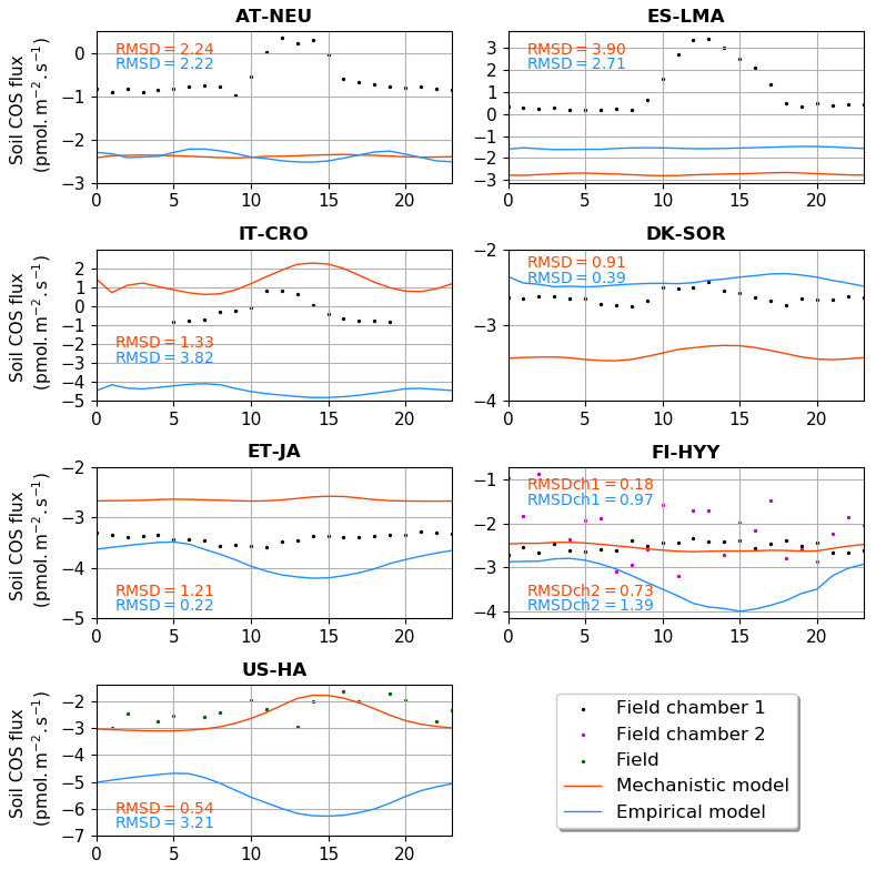
Figure 3Mean diel cycle of net soil COS fluxes (pmol m−2 s−1) over a month at AT-NEU (August 2015), ES-LMA (May 2016), IT-CRO (July 2017), DK-SOR (June 2016), ET-JA (August 2016), FI-HYY (August 2015), and US-HA (July 2012). Soil COS fluxes are computed with a variable atmospheric COS concentration. The observation-based diel cycles (dots) are computed using random forest models at AT-NEU, ES-LMA, IT-CRO, DK-SOR and ET-JA. At AT-NEU and ES-LMA, RMSD values between the simulated and observed fluxes are given with the respective model colour at each site and for both soil chambers at FI-HYY (ch1 and ch2).
The empirical model shows a maximum soil COS uptake around 15:00 at ET-JA, FI-HYY, US-HA, and IT-CRO, which is not found in the observations at FI-HYY and is in contradiction with the observed diel variations at IT-CRO and ES-LMA. Considering all sites, the mechanistic model leads to a smaller error between the simulations and the observations, with a mean RMSD of 1.38 pmol m2 s−1 against 1.87 pmol m2 s−1 for the empirical model.
3.1.3 Dependency on environmental variables
Figure 4 represents simulated net soil COS fluxes versus soil temperature and soil water content at the different sites. At the sites where only a net soil COS uptake is simulated by the mechanistic model (all sites except IT-CRO and ES-LMA), soil COS uptake generally decreases with increasing soil water content, which appears to be the main driver of soil COS fluxes. This behaviour can be explained by a decrease in COS diffusivity through the soil matrix with increasing soil moisture, reducing soil COS availability for microorganism consumption. Furthermore, an optimum soil water content for net soil COS uptake is found between 10 % and 15 %, which was also observed in Ogée et al. (2016) and in several field studies to be around 12 % (Kesselmeier et al., 1999; Liu et al., 2010; van Diest and Kesselmeier, 2008). This optimum soil water content for soil COS uptake is related to a site-specific temperature optimum, which is found between 13 and 15 ∘C at US-HA for example. Indeed, Ogée et al. (2016) also describe a temperature optimum with a value that depends on the studied site (Kesselmeier et al., 1999; Liu et al., 2010; van Diest and Kesselmeier, 2008). At IT-CRO and ES-LMA, where a strong net soil COS production is simulated by the mechanistic model, the main driver of soil COS fluxes becomes soil temperature. At these sites, the net soil COS production increases with soil temperature, due to the exponential response of soil COS production term to soil temperature. The increase in soil COS production with soil temperature at IT-CRO and ES-LMA is supported by the observations (Fig. S1 in the Supplement).
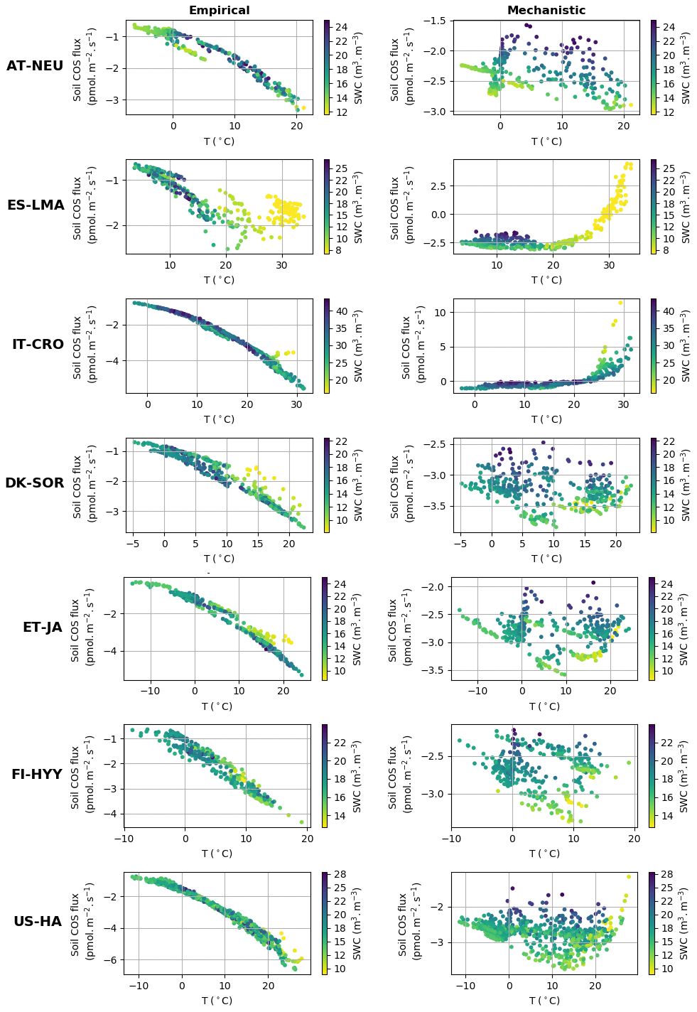
Figure 4Simulated daily average net soil COS flux (pmol m2 s−1) versus soil temperature (∘C) and soil water content (SWC) (m3 m−3) at AT-NEU, ES-LMA, IT-CRO, DK-SOR, ET-JA, US-HA, and FI-HYY, for the empirical and the mechanistic model.
Contrary to the mechanistic model, soil COS uptake computed with the empirical model is mainly driven by soil temperature, with a soil COS uptake that increases with increasing soil temperature. This response of the empirical model to soil temperature is due to its relation to soil respiration, which is enhanced by strong soil temperature. However, this net increase in soil COS uptake with soil temperature at all sites is not found in the observations (Fig. S1). It can be noted that low soil moisture values were found to limit soil COS uptake for the empirical model, as seen at ES-LMA for a soil water content below 8 %.
3.1.4 Sensitivity analyses of soil COS fluxes to parameterization
Sensitivity analyses including a set of parameters (19 for the empirical model and 21 for the mechanistic model) were performed to evaluate the sensitivity of soil COS fluxes to each of the selected parameter. The Morris scores were normalized by the highest values to help rank the parameters by their relative influence on soil COS fluxes, where a score of 1 represents the most important parameter and that of 0 represents the parameters that have no influence on soil COS fluxes. For reasons of clarity, in the following we present the results only for the parameters that were found to have an impact on soil COS fluxes (Morris scores not equal to 0).
Figure 5 shows the results of the Morris sensitivity experiments highlighting the key parameters influencing soil COS fluxes from the empirical and the mechanistic models at FI-HYY and US-HA. For the empirical model at both sites, the first-order parameter (ksoil) is the most important parameter in the computation of soil COS fluxes, as it directly scales soil respiration to soil COS fluxes. The following parameters to which soil COS fluxes are the most sensitive are the scalar on the active soil C pool content (soilC) and the temperature-dependency factor for heterotrophic respiration (soil_Q10). Indeed, the soilC parameter determines the soil carbon active pool content, which can be consumed by soil microorganisms during respiration, therefore impacting soil COS fluxes from the empirical model. The soil_Q10 parameter impacts soil COS fluxes at both sites, as it determines the response of soil heterotrophic respiration to temperature, which is included in the proportionality of soil COS fluxes to the total soil respiration in the empirical model. Similarly, one of the second-order parameters, the minimum soil wetness to limit the heterotrophic respiration (min_SWC_resp), has an impact on soil COS fluxes from the empirical model only. The importance of min_SWC_resp for soil COS fluxes is found at US-HA but not at FI-HYY. This can be explained by the difference in soil moisture between the two sites, with an annual mean of 16.2 % at US-HA and reaching a minimum of only 8.8 % against an annual mean of 17.5 % with a minimum of 12.4 % at FI-HYY.
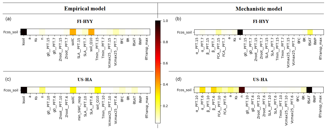
Figure 5Morris sensitivity scores of the key parameters to which soil COS fluxes are sensitive, for the empirical (a, c) and the mechanistic (b, d) models. The two studied sites are FI-HYY (a, b) and US-HA (c, d). Full descriptions of each tested parameter can be found in Tables S3 and S4 in the Supplement. The PFT is indicated at the end of the parameter names for the PFT-dependent parameters (at FI-HYY, PFT 7 is boreal needleleaf evergreen, and PFT 15 is boreal natural C3 grassland; at US-HA, PFT 6 is temperate broadleaf summergreen, and PFT 10 is temperate natural C3 grassland).
Contrary to the empirical model, soil COS fluxes computed with the mechanistic model are more sensitive to two second-order parameters, the van Genuchten water retention curve coefficient n and the saturated volumetric water content (θSAT). These two second-order parameters are strongly linked to soil hydrology and determine the soil water content, which affects COS diffusion through the soil matrix and its uptake. The van Genuchten coefficients occur in the relationships linking hydraulic conductivity and diffusivity to soil water content (van Genuchten, 1980). At both sites, the strong impact of the van Genuchten water retention curve coefficient n on soil COS fluxes simulated with the mechanistic model highlights the critical importance of soil architecture. Thus, soil COS fluxes computed with the mechanistic model are expected to strongly vary according to the different soil types. Then, the first-order parameters (fCA, α, and β) also influence soil COS fluxes from the mechanistic model. However, the uptake parameter (fCA of PFT 15, boreal C3 grass) has the most influence on soil COS fluxes at FI-HYY, while it is the production-related parameter (α of PFT 6, temperate broadleaved summergreen forest) that has the largest impact at US-HA. The stronger influence of the production parameter involved in the temperature response at US-HA might be explained by the difference in temperature between the two sites, which ranges from −10 to 25 ∘C at US-HA with an annual mean of 7.5 ∘C in 2013, while only ranging from −5 to 15 ∘C with an annual mean of 4.3 ∘C at FI-HYY in 2015. Similar to the difference in the main driver of soil COS fluxes found in Fig. 4, the most important first-order parameters to which soil COS fluxes are sensitive seem to differ between uptake and production parameters depending on the site conditions. It is to be noted that at US-HA, the most important production parameters are the ones of the dominant PFT at this site (PFT 6), which also correspond to a stronger response of the production term to temperature than for PFT 10 (temperate C3 grass). However, at FI-HYY the most influential uptake parameter is for PFT 15 (boreal C3 grass) that only represents 20 % of the PFTs at this site, while PFT 7 (boreal needleleaf evergreen forest) is the dominant PFT. This can be explained by the range of variation that is assigned to fCA of PFT 7 by Meredith et al. (2019), which is larger than the one of fCA for PFT 15 (9000 against 3100).
Finally, a set of parameters related to photosynthesis, conductance, phenology, hydrology, and carbon uptake has an impact on soil COS fluxes computed with both the empirical and the mechanistic models at the two sites. The specific leaf area (SLA), maximum rate of Rubisco activity-limited carboxylation at 25 ∘C (Vcmax25), residual stomatal conductance (g0), and minimum photosynthesis temperature (Tmin) have an impact on soil COS fluxes, as they also indirectly affect soil moisture through their influence on transpiration and stomatal opening. The second-order parameters related to soil hydrology (a, Ks, Zroot, θWP, θFC, θR, and θTransp_max) impact the soil water availability, which affects soil respiration for the empirical model and soil COS diffusion and uptake in the mechanistic model. For example, the parameter for the root profile (Zroot) determines the density and depth of the roots and therefore how much water can be taken up by roots.
3.1.5 Soil COS flux optimization
Figure 6 presents soil COS fluxes before and after optimization of the model parameters to better fit the observations at FI-HYY and US-HA. For the mechanistic model, the optimization at the two sites mainly changes the mean value of soil COS fluxes, by reducing the net uptake at US-HA and increasing it at FI-HYY. Similar to the mechanistic model optimization, the posterior soil COS uptake computed with the empirical model is enhanced at FI-HYY and reduced at US-HA. However, at US-HA, the increase in soil COS uptake is only found between April and October, while the winter soil COS fluxes are not impacted by the optimization. Using the optimized parameterization improves the RMSD by 7 % and 5 % at US-HA and by 23 % and 25 % at FI-HYY for the mechanistic and the empirical model, respectively. While it leads to similar posterior RMSD values between the two models at US-HA, the optimization of the mechanistic model gives a lower RMSD than the empirical model at FI-HYY, with 0.54 pmol m−2 s−1 against 0.95 pmol m−2 s−1.

Figure 6Prior and post-optimization net soil COS fluxes (pmol m−2 s−1) for the empirical (a, c) and the mechanistic (b, d) models. The two studied sites are FI-HYY (a, b) in 2015 and US-HA (c, d) in 2013.
At FI-HYY, the difference between prior and posterior soil COS fluxes from the empirical model seems to mainly come from the change in the soil_Q10 value (Fig. E1 in Appendix E). The soil_Q10 value drops from 0.83 to 0.53, which corresponds to a prior Q10 value of 2.29 versus a posterior value of 1.70, decreasing the heterotrophic respiration response to soil temperature. Soil COS fluxes computed with the empirical model were found to be strongly sensitive to soil_Q10 (Fig. 5). The posterior value of this parameter has nearly attained the lower bound of its variation range. Since the range of variation represents the realistic values this parameter can take, we need to be careful about the fact that this parameter is trying to take values close to, or potentially beyond, these meaningful values. Furthermore, the optimization deviates the Q10 value at FI-HYY from the ones calculated in the observations over the measurement period (3.0 for soil chamber 1 and 2.5 for soil chamber 2). We could assume that ksoil should be defined as temperature dependent for linking soil COS flux to soil respiration (Berkelhammer et al., 2014; Sun et al., 2018), instead of being considered a constant. Thus, the optimization of the empirical model could in fact be aliasing the error of ksoil onto soil_Q10 because of the impossibility to account for the temperature dependence of soil COS to the CO2 uptake ratio (Sun et al., 2018). At US-HA, the optimization also leads to a decrease in soil_Q10 but to a lesser extent, with the parameter remaining comfortably within its range of variation.
For the mechanistic model, the optimization reduces the enhancement factor value (fCA) for PFT 10 at US-HA and increases the value of the production parameter α for the dominant PFT (PFT 6). This enhances the reduction in net soil COS uptake, which was slightly overestimated with the prior model parametrization. At FI-HYY, the optimized parameters show higher values of fCA and of α for PFT 15 and of both production parameters (α and β) for the dominant PFT (PFT 7). This increase in both soil COS uptake and production after optimization could correspond to an attempt to better simulate the larger range of variation found in the observations compared to the modelled fluxes.
Finally, the optimization also affects hydrology-related parameters for both models. However, while it improves the simulated water content compared to the observations for the mechanistic model at the two sites (RMSD decreases by 28 % at FI-HYY and 22 % at US-HA), it leads to a degradation at FI-HYY for the empirical model (RMSD increases by more than 3 times). Since the empirical model is quite a simplistic model with few parameters, it relies on parameters from different processes to help better fit the observations – sometimes degrading the fit to the other processes. The mechanistic model is able to both improve the fit to the COS observations and soil moisture values, implying its parameterization is more consistent.
This optimization experiment has been promising, highlighting how observations can be used to improve the models. However, since we only optimized over two sites due to the scarcity of soil COS flux observations, for the global-scale simulations in the rest of this study, we will rely on the default parameter values of each parameterization.
3.2 Global-scale COS fluxes
3.2.1 Soil COS fluxes
The spatial distribution of oxic soil COS fluxes shows a net soil COS uptake everywhere except in India, in the Sahel region, and in some areas in the tropical zone, where net soil COS production is simulated (Fig. 7a). The strongest uptake rates are found in western North America and South America, as well as in China, with a mean maximum uptake of −4.4 pmol COS m−2 s−1 over 2010–2019. The difference in magnitude between the maximum uptake value and the maximum of production can be noticed, with a net production reaching 67.2 pmol COS m−2 s−1 in the Sahel region. India and the Sahel region, where oxic soil COS production is concentrated, are represented in ORCHIDEE by a high fraction of C3 and C4 crops (Fig. S4). In the mechanistic model, crops are associated with the lowest fCA value due to overall lower fungal diversity and abundance in agricultural fields (Meredith et al., 2019) and the strongest response of oxic soil COS production to temperature as observed by Whelan et al. (2016). Thus, these PFT-specific parameters combined with high temperature in the tropical region can explain the net oxic soil COS production found in these regions. C3 crops are also dominant in China near the Yellow Sea (Fig. S4). However, the mean soil temperature in this region is about 15 ∘C lower than the mean soil temperature in India, leading to a lower enhancement of soil COS production. The highest atmospheric COS concentration is also found in this region with about 800 ppt (Fig. S3). Indeed, recent inventories have shown that China was related to strong anthropogenic COS emissions due to industry, biomass burning, coal combustion, agriculture, or vehicle exhaust (Yan et al., 2019; Zumkehr et al., 2018). High atmospheric COS concentrations increase soil COS diffusion and uptake that can compensate part of soil COS production. The highest values of soil COS fluxes for anoxic soils are located in northern India, with a mean maximum value reaching 36.8 pmol COS m−2 s−1 (Fig. 7b). This region is characterized by rice paddies, which were also associated with strong COS production in previous studies (Zhang et al., 2004).
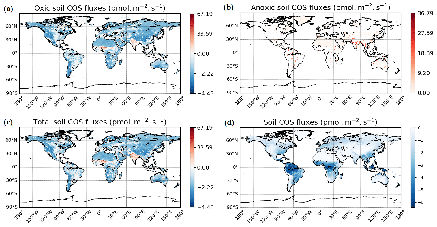
Figure 7Maps of mean soil COS fluxes for the mechanistic (a, b, c) and the empirical model (d), computed over 2010–2019 with a variable atmospheric COS concentration. Colour scales were normalized between the minimum and maximum soil COS flux values and centred on zero for oxic and total soil COS fluxes computed with the mechanistic model. The map resolution is 0.5∘ × 0.5∘.
The total soil COS fluxes (oxic and anoxic) computed with the mechanistic model (Fig. 7c) show a very different spatial distribution than the one obtained with the empirical model (Fig. 7d). Soil COS fluxes from the empirical model are on the same order of magnitude for net COS uptake than the mechanistic model, with a mean maximum uptake of −6.41 pmol COS m−2 s−1. However, most soil COS uptakes simulated by the empirical model is located in the tropical region, where soil respiration is strong due to high temperature. The distribution and magnitude of soil COS flux from the empirical approach is similar to the one presented in Kooijmans et al. (2021) (see Fig. S15 in the Supplement of Kooijmans et al., 2021), when implemented in SiB4. For the mechanistic model, the comparison of oxic soil COS flux distribution with the one in SiB4 shows a net soil COS emission in India in both SiB4 and ORCHIDEE. However, the maximum oxic soil COS flux is about 60 pmol m−2 s−1 higher in ORCHIDEE than in SiB4. The regions with the strongest net oxic soil COS uptake also differ between SiB4 and ORCHIDEE, as it is concentrated in the tropics in SiB4, as well as in western North America and South America, and in China for ORCHIDEE.
The difference in soil COS fluxes between the mechanistic model and the empirical model ranges from −4.1 pmol COS m−2 s−1 to +68.0 pmol COS m−2 s−1 (Fig. D1 in Appendix D). Over western North America and South America; northern and southern Africa; western Asia; and eastern, northern, and central Asia, the net COS uptake from the mechanistic model exceeds the uptake from the empirical model. On the contrary, soil COS uptake from the empirical approach is higher than the net COS uptake simulated with the mechanistic model over eastern North America and South America; western, central, and eastern Africa; and Indonesia. The absence of soil COS production representation in the empirical approach leads to the strongest differences in India and in the Sahel region, reaching +68.0 pmol COS m−2 s−1.
3.2.2 Temporal evolution of the soil COS budget
We computed the mean annual soil COS budget over the period 2010–2019 using the monthly variable atmospheric COS concentration, and we compared its evolution to the variations in the mean annual atmospheric COS concentration.
The evolution of the mean annual soil COS budget (Fig. 8) shows small variations in the budget for oxic soils computed with the mechanistic model between 2010 and 2015, with a net sink ranging from −133 to −124 GgS yr−1. Then, from 2016 we see a sharp decrease in this budget, which reaches −98 GgS yr−1 in 2019. This decrease also corresponds to the decrease in atmospheric COS concentration observed between 2016 and 2019 with a loss of 25 ppt in 3 years. Several monitoring stations recorded a drop in atmospheric COS concentration over Europe, as for the Gif-sur-Yvette station with −42 ppt between 2015 and 2021 (updated after Belviso et al., 2020). Note that the decrease in the oxic soil COS budget computed with the mechanistic model is sharper than the drop in atmospheric COS concentration because changes in oxic soil COS budget result from the combined effect of decreasing atmospheric COS concentration and changes in the drivers of soil COS fluxes (i.e. changes in soil temperature and water content during the 10-year period which are not homogenously distributed around the globe; not shown). On the contrary, the soil COS net uptake computed with the empirical model slightly increases from −212 GgS yr−1 in 2010 to −219 GgS yr−1 in 2019. As the empirical model defines soil COS flux as proportional to the total soil respiration independently of atmospheric COS concentration, the budget obtained with this model is not impacted by the variations observed in atmospheric COS concentration. The anoxic soil COS budget follows soil temperature variations (not shown), with an increasing trend of about 0.17 GgS yr−1 over the studied period.
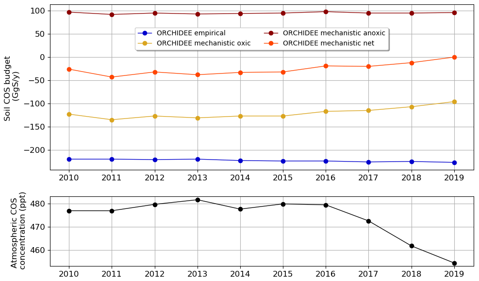
Figure 8Evolution of mean annual soil COS budget and mean annual atmospheric COS concentration between 2010 and 2019, computed with a variable atmospheric COS concentration.
3.3 Transport and site-scale concentrations
3.3.1 Interhemispheric gradient
We transported total COS fluxes for the different configurations (i.e. including not only the soil fluxes but also other components of the COS atmospheric budget, listed in Table 2) with the LMDZ6 atmospheric transport model as described in Sect. 2.1.3. We analysed COS concentrations derived from simulated COS fluxes obtained with the mechanistic and two empirical approaches with regards to the COS concentrations observed at 14 NOAA sites depicted in Fig. B1 in Appendix B. Note that atmospheric mixing ratios of COS result from the transport of all COS sources and sinks and that, due to other sources of errors (transport and errors in the other COS fluxes), the comparison presented in the following should be taken as a sensitivity study of COS seasonal cycle and interhemispheric gradient to the soil exchange fluxes rather than a complete validation of one approach or the other. Figure 9 shows the COS atmospheric concentrations at NOAA sites as a function of latitude for each simulated soil flux and for the observations. Here as we want to focus on the latitudinal variations in atmospheric COS mixing ratios; the atmospheric COS concentrations have been vertically shifted to have the same mean as the observations. This means that the concentrations values cannot be compared at each site; we can only compare the interhemispheric gradients of simulated and observed concentrations. The RMSD for the mechanistic model with oxic soils only, the mechanistic model with oxic and anoxic soils, the empirical Berry model (with oxic soils only), and the empirical Launois model (with oxic and anoxic soils) are 36.5, 39.4, 43.0, and 51.0 ppt, respectively. While the different approaches show similar gradient patterns in the southern latitudes, they lead to strong differences in the simulated concentrations in the Northern Hemisphere. Compared to empirical approaches, the mechanistic approach marginally improves the latitudinal distribution of the atmospheric mixing ratios by decreasing the concentrations in the high latitudes. The lower atmospheric mixing ratios above 60∘ N reflect the stronger soil absorption in the mechanistic model (see Fig. 9), where soil COS uptake is dominant and the compensation by COS production is small (Fig. D2 in Appendix D). Despite this slight improvement, there are persistent biases as overestimated concentrations at the high-latitude sites ALT, BRW, and SUM and underestimated concentrations at most tropical sites, i.e. WIS, MLO, and SMO. These model–observation mismatches have led top-down studies to identify vegetation as an underestimated sink in the high latitudes (Ma et al., 2021; Remaud et al., 2022) and the tropical oceanic emissions as the missing source (Berry et al., 2013; Launois et al., 2015; Kuai et al., 2015; Ma et al., 2021; Remaud et al., 2022; Davidson et al., 2021). The present anoxic soil fluxes have little impact on the surface latitudinal distributions and therefore are unlikely to shed new light on the tropical missing source. An explanation for the small impact is that they are located outside areas experiencing deep convection events (e.g. the Indian monsoon domain), and thus the surface concentrations are less sensitive to these fluxes.

Figure 9Comparison of the latitudinal variations in the COS abundances simulated by LMDZ at NOAA sites with the observations (black). The LMDZ COS abundances have been vertically shifted such that the means of the simulated concentrations are the same as the mean of the observations. The error bars around the black curve represent the standard deviation over the whole studied period at each NOAA site. The orange curve is obtained using the oxic soil fluxes of the mechanistic model. The red curve is obtained using the oxic and anoxic soil fluxes of the mechanistic model. The blue curve is given by LMDZ using the oxic soil fluxes from the Berry empirical model. The green curve is obtained using the soil fluxes from the empirical approach of Launois et al. (2015). For more clarity, the names of the stations KUM (19.74∘ N, 155.01∘ W), NWR (40.04∘ N, 105.54∘ W), LEF (45.95∘ N, 90.28∘ W), and SUM (72.6∘ N, 38.42∘ W) are not shown in this figure due to their proximity to other stations (Fig. B1 and Table B1 in Appendix B).
3.3.2 Seasonal cycle at NOAA sites
Figure 10 shows the detrended temporal evolution of COS concentrations for the mechanistic and empirical approaches at Alert (ALT, Canada) and Harvard Forest (HFM, USA). Because of the mean westerly flow, the HFM site is influenced by continental regions to the west (Sweeney et al., 2015) and is more sensitive to the soil fluxes than other mid-latitude sites located to the west of the ocean as MHD; see Fig. 1 in Remaud et al. (2022). The ALT site samples air masses come not only from high-latitude ecosystems (Peylin et al., 1999) but also from regions further south due to atmospheric transport (Parazoo et al., 2011). The reader is referred to Table B2 in Appendix B for the other sites. At both sites, the mechanistic approach tends to weaken the total seasonal amplitude and increase the model–data mismatch. At HFM, since the mechanistic soil model shows overall good agreement with the observed soil fluxes (e.g. Fig. 2), the model–observation mismatch likely arises from errors in other components of the COS budget (in particular oceanic and vegetation fluxes). Therefore, empirical approaches give a more realistic seasonality of atmospheric concentrations for the wrong reasons, which likely hides an underestimated vegetation uptake. Indeed, as Maignan et al. (2021) showed that the vegetation uptake magnitude in ORCHIDEE was consistent with measurements, the introduction of variable atmospheric COS concentrations decreased the vegetation uptake, which, as a result, is very likely underestimated now. Moreover, the comparison between simulated and observed concentrations shows a degradation of the simulated concentrations in this study compared to Maignan et al. (2021). It is to be noted that in addition to using a variable atmospheric COS concentration in this study, the transported ocean COS fluxes from Masotti et al. (2016) and Lennartz et al. (2017, 2021) differ from the ones used in Maignan et al. (2021), Kettle et al. (2002), and Launois et al. (2015). These results illustrate the necessity of well constraining both the soil and vegetation fluxes in order to optimize the GPP with the help of atmospheric inverse modelling.
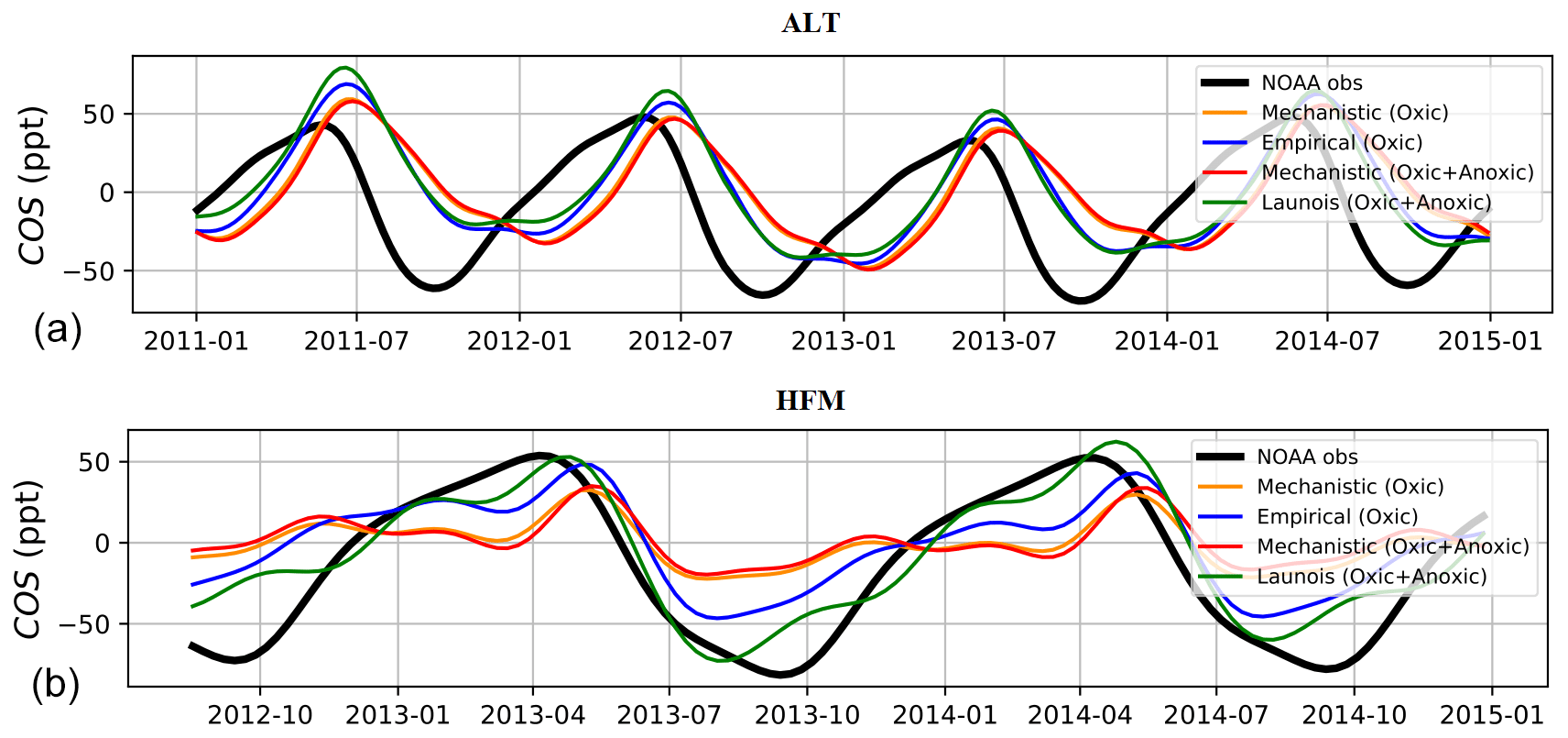
Figure 10Detrended temporal evolution of simulated and observed COS concentrations at two selected sites, simulated with LMDZ6 transport between 2011 and 2015. The simulated concentrations are obtained by transporting the surface fluxes described in Table 2 and changing only the contribution from soils, with mechanistic (oxic soils alone and oxic + anoxic soils) and empirical approaches (Berry et al., 2013; Launois et al., 2015). (a) Alert station (ALT, Canada) and (b) Harvard Forest station (HFM, USA). The curves have been detrended beforehand and filtered to remove the synoptic variability (see Sect. 2.3.3). Please note that the date format in this figure is year-month.
4.1 Soil budget
According to the mechanistic approach of this study, the COS budget for oxic soil is a net sink of −126 GgS yr−1 over 2009–2016, which is close to the value of −130 GgS yr−1 found by Kettle et al. (2002) (Table 3). This net COS uptake by oxic soils is higher than the one found in SiB4 by Kooijmans et al. (2021) with −89 GgS yr−1, also based on the mechanistic model described in Ogée et al. (2016). In SiB4 and in ORCHIDEE, the mechanistic model gives the lowest oxic soil COS net uptake compared to all previous studies, which were using empirical approaches. This budget is also 41 % lower than the one found with the Berry empirical approach in this study, with an uptake of −214 GgS yr−1. The anoxic soil COS budget computed with the mechanistic approach is +96 GgS yr−1, which is close to the budget found by Launois et al. (2015) of +101 GgS yr−1 based on methane emissions. However, while COS emissions from anoxic soils were only located in the northern latitudes in Launois et al. (2015), the COS production in this study is also distributed in the tropical region. Thus, we can expect that despite similar budget values for anoxic soils, the difference in flux distribution will impact the latitudinal gradient of COS fluxes. Finally, adding the anoxic soil COS budget to oxic soil COS budget results in a total soil COS budget of only −30 GgS yr−1 for the mechanistic approach.
When computing the net total COS budget considering all sources and sinks of COS (Table 2), we found that neglecting the potential COS production of oxic soils and COS emissions from anoxic soils leads to an overestimation of COS sink or an underestimation of COS source to close the budget (−165 GgS yr−1). On the contrary, the total COS budget computed with the mechanistic soil model is closed given the uncertainties on each component (Table 2). However, despite a closed budget, the mismatch between the observed and simulated latitudinal gradients of atmospheric COS concentration highlights errors in COS flux component distributions (Fig. 9).
It is also to be noted that the mechanistic model better simulates the lack of seasonality in the soil COS flux at US-HA compared to the empirical model (Fig. 2). US-HA is represented by 80 % of PFT 6 (temperate broadleaved summergreen forest), and the absence of seasonality by this PFT has also been reported at a mid-latitude site at Gif-sur-Yvette (Belviso et al., 2020). This PFT is largely found in the temperate region such as in Europe and in the southern United States. Moreover, NWR, HFM, and LEF stations are mainly influenced by COS exchanges from PFT 6. Therefore, the use of the mechanistic model would be recommended to carry out new comparisons at these mid-latitude sites.
4.2 Variable atmospheric COS concentration versus constant atmospheric COS concentration
We studied the impacts of using a constant versus a variable atmospheric COS concentration on soil COS fluxes. At the site scale we found a distinction between the sites where soil COS production is strong (IT-CRO and ES-LMA) and the sites mainly showing a net soil COS uptake. The impact of using a constant atmospheric COS concentration is lower at IT-CRO and ES-LMA because the atmospheric COS concentration does not directly impact the soil COS production term but participates in the net soil COS flux. Our study shows that at the sites where a net soil COS uptake is dominant, using a constant atmospheric COS concentration leads to a lower soil COS flux in winter and a higher soil COS flux from spring to autumn (not shown). Indeed, during the growing season, plant uptake decreases atmospheric COS concentration (Fig. S2), which reduces COS availability for soil COS diffusion, whereas during winter, a higher atmospheric COS concentration enhances COS diffusion into the soil.
At the global scale, as the variable atmospheric COS concentration used in this study shows a decrease of about 25 ppt in the recent years (Fig. 8), considering a constant atmospheric COS concentration would not enable the representation of the impact of this strong variation on soil COS fluxes. When computing the soil COS budget over 2016 to 2019, we found a net uptake of −126 GgS yr−1 with the mechanistic model using a constant atmospheric COS concentration against the −110 GgS yr−1 computed with a monthly spatially variable concentration. Using a constant atmospheric COS concentration would then lead to a 13 % higher net soil COS uptake over the past 4 years.
We also studied the impact of considering a constant versus a variable atmospheric COS concentration on the seasonal variations in mean monthly soil COS fluxes over 2010–2019, simulated with the mechanistic model (not shown). We found that using a constant atmospheric COS concentration leads to an increase in net soil COS uptake over the whole year in the southern latitudes and from June to February in the northern latitudes (reaching 1.62 pmol m−2 s−1). This increase is higher over the regions with the lowest atmospheric COS concentrations, which limits COS diffusion through the soil matrix. On the contrary when atmospheric COS concentration is high in the northern latitudes between April and May, considering a constant atmospheric COS concentration decreases the net soil COS uptake. We notice that this lower net soil COS uptake with a constant atmospheric COS concentration can be found as early as March over Europe, where atmospheric COS concentration is higher in this region. In eastern Asia, where atmospheric COS concentration is higher than 800 ppt, the decrease in the net soil COS uptake can reach −2.34 pmol m−2 s−1 when considering a constant atmospheric COS concentration.
It is to be noted that the modelled COS concentrations we used have their own uncertainty, which is however smaller than their difference with the fixed value (Remaud et al., 2022).
4.3 Foreseen improvements
The mechanistic representation of soil COS fluxes was found to be in better agreement with the observations at field sites. However, there can be strong differences between the simulated fluxes and the observations at some sites, especially at AT-NEU and ES-LMA. In the mechanistic approach, the influence of light on soil COS fluxes is not considered. Several field studies have reported light-induced emissions in oxic soils (Kitz et al., 2017; Meredith et al., 2018; Spielmann et al., 2019a; Whelan and Rhew, 2015), assumed to be related to the effect of light on soil organic matter. Spielmann et al. (2019a) related strong soil COS emissions during daytime to light at the sites where direct solar radiations reached the surface, such as ES-LMA and AT-NEU. At these sites, the mechanistic model was unable to represent the soil COS emission peak during daytime. The optimization we performed showed that, as expected, adjusting the parameters to site observations improves the fit between the simulated and observed fluxed. However, it is necessary to represent all important processes in the mechanistic approach before calibrating the parameters. Thus, a next step in our modelling approach could be to include the light influence on soil COS fluxes, which can be of major importance for the sites where radiations strongly affect soil COS fluxes. Several studies also found that soil COS production could be related to nitrogen content, which increases with nitrogen fertilizer application (Kaisermann et al., 2018; Meredith et al., 2018, 2019). At the sites where soil is enriched with nitrogen inputs, such as agricultural fields or managed and fertilized grasslands and forests, the fertilization practices would also need to be included when representing the dynamics of soil COS fluxes. However, the soil nitrogen content and soil microbial nitrogen biomass vary not only with fertilization but also with location. Then, in addition to indications on land use, information on the total soil nitrogen content should be included in the model to consider nitrogen impact on soil COS flux. In the soil COS models, the impact of snow cover is also not represented. Indeed, due to the scarcity of soil COS flux observations in winter and with snow cover, its effect on soil COS flux could not be implemented in soil COS models yet. However, Helmig et al. (2009) found that COS uptake was not zero when soil is covered by snow at Niwot Ridge, Colorado.
Moreover, one difficulty with the study of soil COS fluxes arises from the scarcity of field measurements that could be used for model validation and calibration. Besides, the observation sites considered here are all located in a small latitudinal range between 39 and 62∘ N. Measurements in the tropics and in the Southern Hemisphere are needed. Especially, soil COS flux observations in northern India could help to validate the net soil COS production simulated in both SiB4 and ORCHIDEE. In the tropical rainforest, soil COS flux measurements were performed at La Selva Biological Station in Costa Rica (Sun et al., 2014). When available, these measurements could allow for a first comparison between the observed and simulated soil COS flux in a tropical region.
Then, the characterization of the soil microbial community should also be addressed to improve the scaling of CA content and activity, represented by the fCA parameter (Meredith et al., 2019).
The implementation of the soil COS flux mechanistic model from Ogée et al. (2016) in SiB4 (Kooijmans et al., 2021) shows a seasonal cycle with a maximum net soil COS uptake in summer for the sites without crops, while the fluxes computed in ORCHIDEE show almost no seasonality. The expression of the production term P differs between the two models, which is based on Meredith et al. (2018) in SiB4 and on Whelan et al. (2016) in ORCHIDEE. The observation sites that are common to the two studies (FI-HYY, US-HA, AT-NEU, and DK-SOR) are also represented by different fractions of biomes between SiB4 and ORCHIDEE, which changes the parameterization to compute soil COS fluxes. Finally, the parameter values for the enhancement factor fCA for grass differ as the value for tropical grass is also assigned to C3 and C4 grass in SiB4. Soil COS flux field data are mainly available in summer; therefore having field measurements over a whole year could better inform the seasonality of observed soil COS fluxes to compare to the simulations.
The optimization does not modify the respective seasonality of both soil COS models, with a seasonal cycle that agrees with the one of soil respiration for the empirical model and a lack of seasonality for the mechanistic model. The lack of observations in winter does not enable validating or constraining soil COS fluxes in winter. Therefore, having field observations over a whole year could help to determine if both models could be calibrated with a constraint over the whole year instead of only during summer and autumn. Moreover, the optimized set of parameters for the empirical models leads to a degradation of the simulated soil water content compared to the observations at FI-HYY, while the optimized parameters of the mechanistic model improve the representation of soil water content at US-HA and FI-HYY. Thus, the mechanistic approach is to be preferred over the empirical model and should be selected for future COS studies in ORCHIDEE.
The sensitivity analyses showed the importance of the hydrology-related parameters in the computation of soil COS fluxes with the mechanistic model. Thus, assuming an accurate representation of soil COS fluxes, soil COS fluxes could have the potential to add a new constraint on hydrology-related parameters.
In this work, soil COS fluxes are computed in the top 9 cm, which assumes that soil COS uptake and production depend on the conditions in the first soil layers. Indeed, soil COS uptake depends on diffusive supply of COS from the atmosphere. However, since soil COS production does not depend on COS supply, deeper soil layers could also contribute to soil COS production. A study by Yang et al. (2019) presents COS profile measurements in an orchard, which shows a non-zero COS concentration in deeper soil layers but no direct evidence for attributing it to soil COS production. Thus, we could consider deeper soil layers in the future to study the impact on soil COS fluxes compared to considering only the top soil layers.
The anoxic soil map of regularly flooded wetlands from Tootchi et al. (2019) enables approximating the spatial distribution of anoxic soil. However, in our approach, seasonality is only represented through soil temperature seasonality. Anoxic soil temporal dynamics were initially included in the model described by Ogée et al. (2016) with the soil redox potential but is not implemented in land surface models such as ORCHIDEE yet. We could also refine our approach by distinguishing between the different types of wetlands and define a Pref value for each wetland type instead of a global value of 10 pmol COS m−2 s−1. Then, a distinction could also be made for anoxic soil COS fluxes from boreal peatlands, as Meredith et al. (2019) give a value of fCA specific to this biome. Moreover, indirect COS emissions from DMS oxidation in anoxic soils have been reported (Kettle et al., 2002; Watts, 2000) but are not represented in this study. Finally, the anoxic map used here represents 9.7 % of the global land area, but the distribution of anoxic soils can greatly vary depending on the study (between 3 % and 21 %, Tootchi et al., 2019). Therefore, it would also be interesting to investigate the impact of anoxic soil coverage on soil COS flux uncertainty.
We have implemented in the ORCHIDEE LSM a mechanistic and an empirical model for simulating soil COS fluxes. The mechanistic model, which performs a spatialization of the Ogée et al. (2016) model, enables us to consider that oxic soils can be net COS producers, as illustrated at some of the observation sites. The interhemispheric gradient of the COS surface atmospheric mixing ratio is marginally improved when all known COS sources and sinks are transported with the LMDZ model. This study also highlights the sensitivity of simulated atmospheric COS concentrations to soil COS flux representation in the northern latitudes. Thus, the uncertainty in soil COS fluxes could complicate GPP estimation using COS in the Northern Hemisphere.
The soil COS budget at the global scale over the 2009–2016 period is −30 GgS yr−1, resulting from the contribution of oxic soils that represent a net sink of −126 GgS yr−1 and of anoxic soils that represent a source of +96 GgS yr−1. It is to be noted that the contribution from anoxic soils, while leading to a global budget similar to Launois et al. (2015), has a different spatial distribution based on the repartition of regularly flooded wetlands from Tootchi et al. (2019). This repartition seems more accurate, as it also includes anoxic soil COS flux in the tropical region and considers a larger variety of anoxic soils, such as salt marshes and rice paddies.
During this work, we have also shown the importance of considering spatially and temporally variable atmospheric COS concentrations on soil COS fluxes, with an especially large impact at the global scale. This result evidences the impact of the recently decreasing atmospheric COS concentrations on the estimated soil COS fluxes.
Regarding the ORCHIDEE model, we performed a sensitivity study highlighting the key parameters to optimize for the soil models. The impact of soil model parameter optimization was studied at two sites. This study exhibited strong arguments in favour of the mechanistic model, as performing an optimization of the empirical model parameters can lead to aliasing errors and a degradation of the simulated soil water content. A larger database of COS flux measurements at the site scale and especially full year time series would greatly help for the next step, which would be to optimize the parameters of ecosystem COS fluxes.
Table A1Carbonic anhydrase enhancement factor adapted to ORCHIDEE biomes.
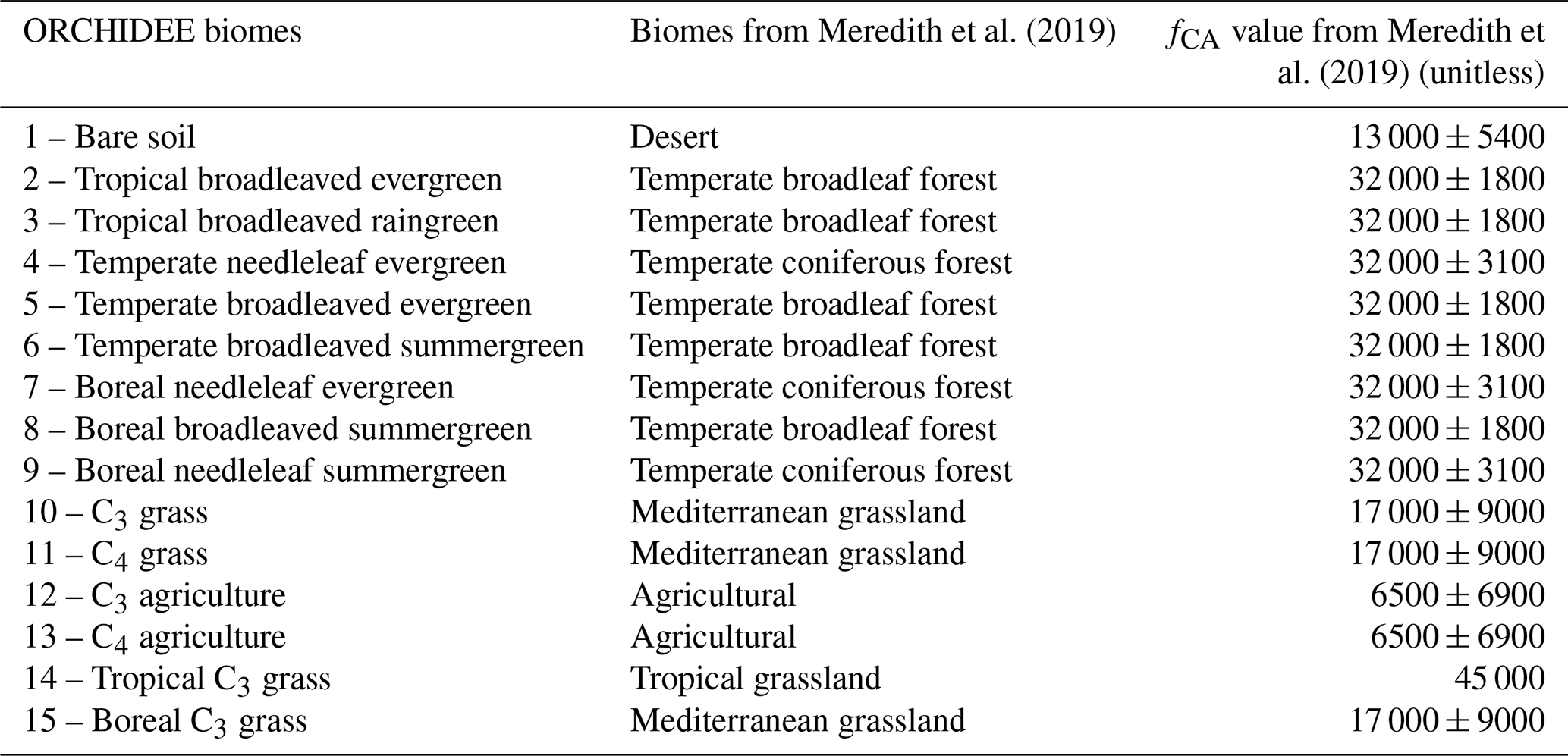
Table A2α and β parameters for COS production term adapted to ORCHIDEE biomes.
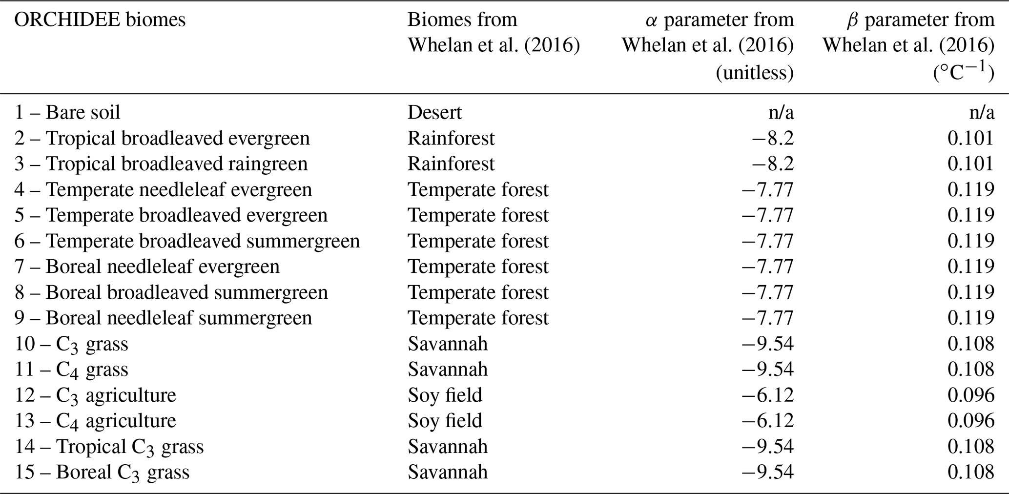
n/a – not applicable.
Table A3Variables for the empirical and mechanistic COS soil models.
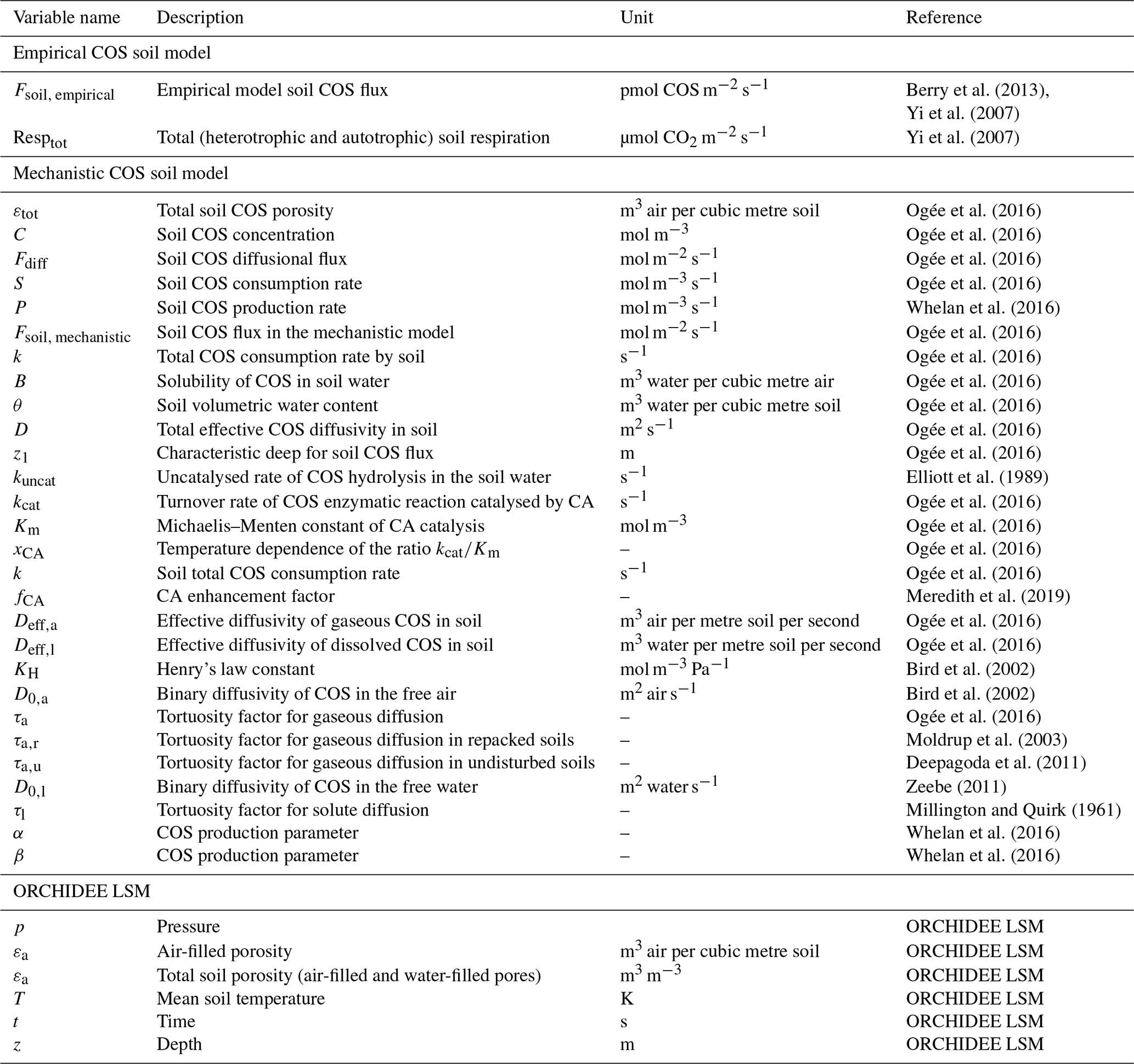
Table A4Constants for the empirical and mechanistic COS soil models.
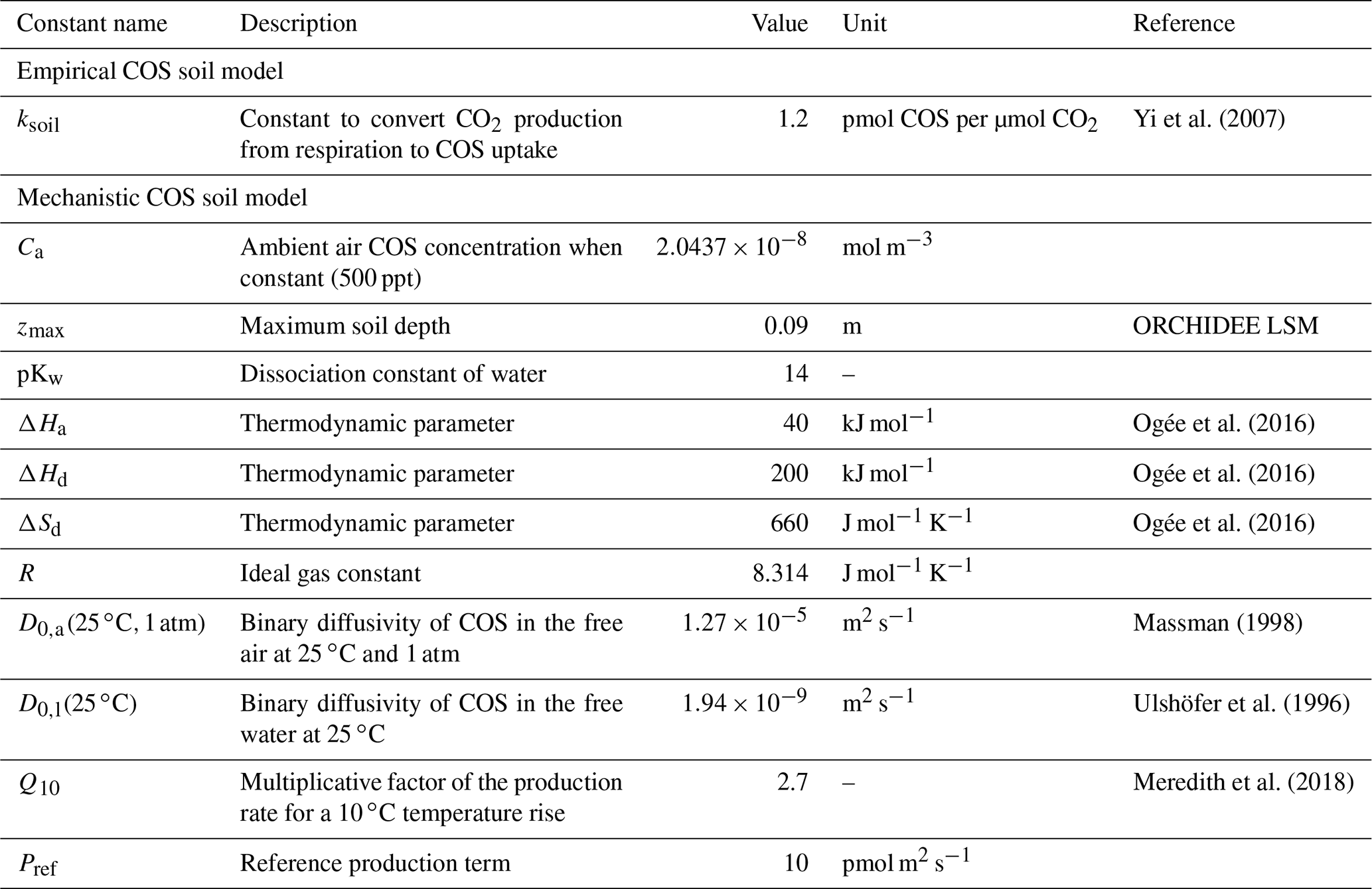

Figure B1Locations of the observation sites for soil COS flux measurements (red) and atmospheric concentration measurements (blue).
Table B1List of air sampling sites selected for evaluation of COS concentrations.

Table B2Normalized standard deviations (NSDs) of the simulated concentrations by the observed concentrations. Within brackets are the Pearson correlation coefficients (r) between simulated and observed COS concentrations for the mechanistic and empirical approaches, calculated between 2011 and 2015 at selected NOAA stations. For each station, NSD and r values closest to one are in bold, and the farthest ones are in italic. The time series have been detrended beforehand and filtered to remove the synoptic variability (see Sect. 2.3.3).
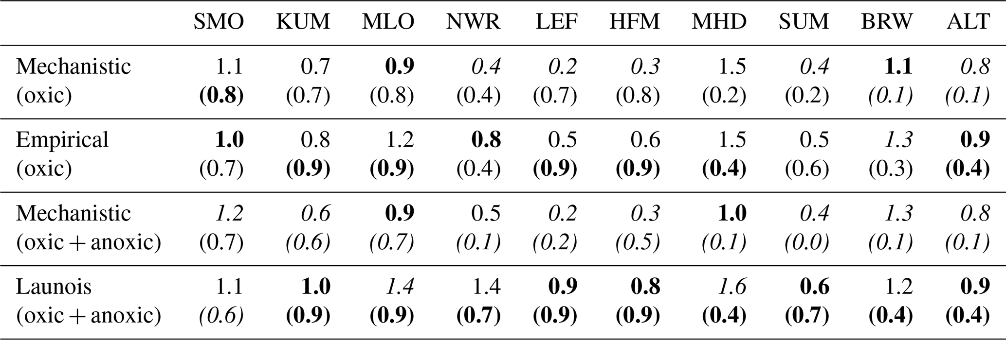
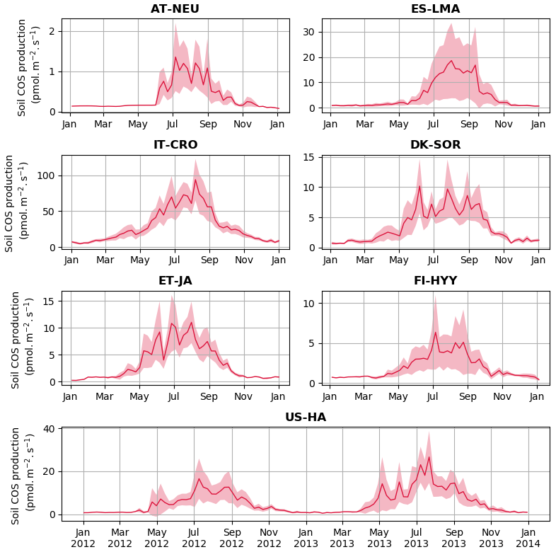
Figure C1Seasonal cycles of soil COS production with weekly average production at AT-NEU, ES-LMA, IT-CRO, DK-SOR, ET-JA, FI-HYY, and US-HA. The shaded areas above and below the modelled curve represent the standard deviation over a week. Soil COS production was computed with a variable atmospheric COS concentration.
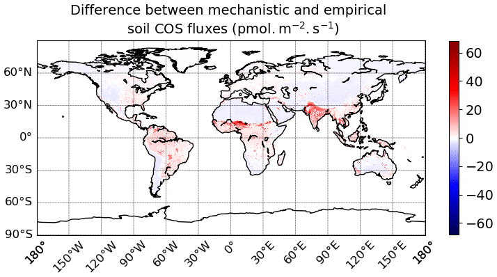
Figure D1Mean difference between soil COS fluxes computed with the mechanistic and the empirical model over 2010–2019. The map resolution is 0.5∘ × 0.5∘.
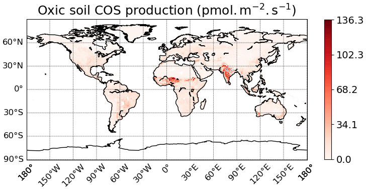
Figure D2Mean spatial distribution of oxic soil COS production term over 2010–2019. The map resolution is 0.5∘ × 0.5∘.
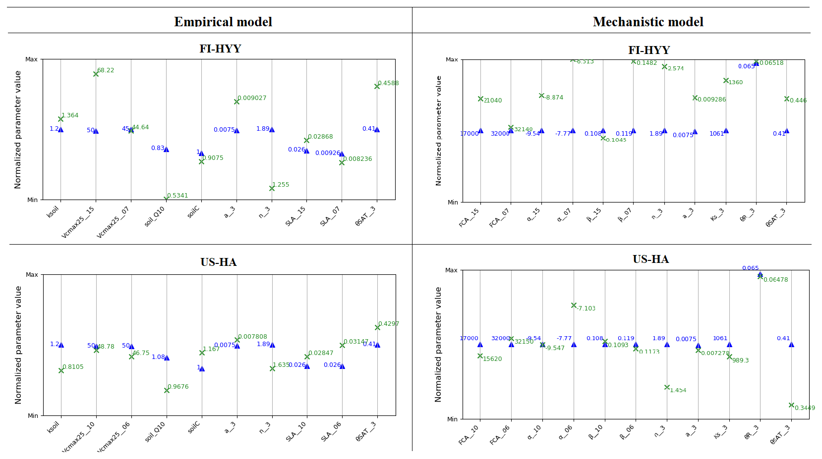
Figure E1Comparison between prior and post-optimization parameter values at FI-HYY and US-HA. The y axis represents the normalization between the edges of the range of variation for each parameter. Prior values of the parameters are represented in blue, and post-optimization values are in green.
The CMIP6 version of the ORCHIDEE model including the soil COS sub-models is available on request to the authors. The LMDZ model is available at http://svn.lmd.jussieu.fr/LMDZ/LMDZ6/ (Laboratoire de Météorologie Dynamique, 2021) under the CeCILL (CEA CNRS INRIA Logiciel Libre) v2 free software license.
For FI-HYY, we used the 2015 soil chamber COS measurements described in Sun et al. (2017), which can be found at https://doi.org/10.15146/R39P4R or in Zenodo at https://doi.org/10.5281/zenodo.322936. For US-HA, we used the soil COS flux data derived from eddy covariance COS and CO2 measurements and soil chamber CO2 measurements conducted in 2012 and 2013 as described in Wehr et al. (2017). We used the COS flux data published in Kitz et al. (2020; https://doi.org/10.5281/zenodo.3664784, Kitz, 2020) and Spielmann et al. (2019a; https://doi.org/10.5281/zenodo.2586891, Spielmann et al., 2019b) for AT-NEU in 2015, DK-SOR and ES-LMA in 2016, and IT-CRO in 2017.
The supplement related to this article is available online at: https://doi.org/10.5194/bg-19-2427-2022-supplement.
CA, FM, MR, and PP conceived the research. JO advised regarding the spatialization of his mechanistic model. CA and FM coded the ORCHIDEE developments and made the simulations. MR transported all COS sinks and sources with the LMDZ model. FK, FMS, and GW provided the data for AT-NEU, ES-LMA, DK-SOR, IT-CRO, and ET-JA. WS provided the data for the FI-HYY site, and RW provided them for the US-HA site. NR provided code and guidance for the sensitivity analysis and data assimilation experiments. SB, JEC, MEW, DH, STL, US, and DM were consulted on their respective expertise.
The contact author has declared that neither they nor their co-authors have any competing interests.
Publisher's note: Copernicus Publications remains neutral with regard to jurisdictional claims in published maps and institutional affiliations.
The authors thank the reviewers for their insightful and useful comments which helped to improve this study. The authors are very grateful to everyone who participated in field data collection used in this study. We thank Vladislav Bastrikov for providing the ORCHIDAS code. We also acknowledge Nicolas Vuichard for providing the soil bulk density map used in ORCHIDEE simulations. Operation of the US-HA site is supported by the AmeriFlux Management Project with funding by the US Department of Energy's Office of Science (contract no. DE-AC02-05CH11231), and additionally it is a part of the Harvard Forest Long Term Ecological Research (LTER) site supported by the National Science Foundation (grant no. DEB-1832210). The field campaign at DK-SOR was supported by the Danish ICOS contribution (ICOS/DK) and by the Independent Research Fund Denmark (grant no. DFF-1323-00182).
This research has been mainly supported by the 4C project of the European Commission's Horizon 2020 framework programme (grant no. 821003) and to a small extent by VERIFY (grant no. 776810).
Florian Kitz, Felix M. Spielmann, and Georg Wohlfahrt were supported by the Austrian Science Fund (FWF) (contract nos. P26931, P27176, P31669, and I03859) and the University of Innsbruck.
This paper was edited by Sönke Zaehle and reviewed by two anonymous referees.
Aneja, V. P., Overton, J. H., and Aneja, A. P.: Emission survey of biogenic sulfur flux from terrestrial surfaces, JAPCA J. Air Waste Ma., 31, 256–258, https://doi.org/10.1080/00022470.1981.10465218, 1981.
Bastrikov, V., MacBean, N., Bacour, C., Santaren, D., Kuppel, S., and Peylin, P.: Land surface model parameter optimisation using in situ flux data: comparison of gradient-based versus random search algorithms (a case study using ORCHIDEE v1.9.5.2), Geosci. Model Dev., 11, 4739–4754, https://doi.org/10.5194/gmd-11-4739-2018, 2018.
Belviso, S., Schmidt, M., Yver, C., Ramonet, M., Gros, V., and Launois, T.: Strong similarities between night-time deposition velocities of carbonyl sulphide and molecular hydrogen inferred from semi-continuous atmospheric observations in Gif-sur-Yvette, Paris region, Tellus B, 65, 20719, https://doi.org/10.3402/tellusb.v65i0.20719, 2013.
Belviso, S., Lebegue, B., Ramonet, M., Kazan, V., Pison, I., Berchet, A., Delmotte, M., Yver-Kwok, C., Montagne, D., and Ciais, P.: A top-down approach of sources and non-photosynthetic sinks of carbonyl sulfide from atmospheric measurements over multiple years in the Paris region (France), PLOS ONE, 15, e0228419, https://doi.org/10.1371/journal.pone.0228419, 2020.
Berkelhammer, M., Asaf, D., Still, C., Montzka, S., Noone, D., Gupta, M., Provencal, R., Chen, H., and Yakir, D.: Constraining surface carbon fluxes using in situ measurements of carbonyl sulfide and carbon dioxide, Global Biogeochem. Cy., 28, 161–179, https://doi.org/10.1002/2013GB004644, 2014.
Berry, J., Wolf, A., Campbell, J. E., Baker, I., Blake, N., Blake, D., Denning, A. S., Kawa, S. R., Montzka, S. A., Seibt, U., Stimler, K., Yakir, D., and Zhu, Z.: A coupled model of the global cycles of carbonyl sulfide and CO2: A possible new window on the carbon cycle, J. Geophys. Res.-Biogeo., 118, 842–852, https://doi.org/10.1002/jgrg.20068, 2013.
Bird, B., Stewart, W., and Lightfoot, E.: Transport Phenomena, John Wiley and Sons, Chemical Engineering Department, University of Wisconsin-Madison, 2002.
Boucher, O., Servonnat, J., Albright, A. L., Aumont, O., Balkanski, Y., Bastrikov, V., Bekki, S., Bonnet, R., Bony, S., Bopp, L., Braconnot, P., Brockmann, P., Cadule, P., Caubel, A., Cheruy, F., Codron, F., Cozic, A., Cugnet, D., D'Andrea, F., Davini, P., de Lavergne, C., Denvil, S., Deshayes, J., Devilliers, M., Ducharne, A., Dufresne, J. L., Dupont, E., Éthé, C., Fairhead, L., Falletti, L., Flavoni, S., Foujols, M. A., Gardoll, S., Gastineau, G., Ghattas, J., Grandpeix, J. Y., Guenet, B., Guez, L. E., Guilyardi, E., Guimberteau, M., Hauglustaine, D., Hourdin, F., Idelkadi, A., Joussaume, S., Kageyama, M., Khodri, M., Krinner, G., Lebas, N., Levavasseur, G., Lévy, C., Li, L., Lott, F., Lurton, T., Luyssaert, S., Madec, G., Madeleine, J. B., Maignan, F., Marchand, M., Marti, O., Mellul, L., Meurdesoif, Y., Mignot, J., Musat, I., Ottlé, C., Peylin, P., Planton, Y., Polcher, J., Rio, C., Rochetin, N., Rousset, C., Sepulchre, P., Sima, A., Swingedouw, D., Thiéblemont, R., Traore, A. K., Vancoppenolle, M., Vial, J., Vialard, J., Viovy, N., and Vuichard, N.: Presentation and Evaluation of the IPSL-CM6A-LR Climate Model, J. Adv. Model. Earth Sy., 12, e2019MS002010, https://doi.org/10.1029/2019MS002010, 2020.
Brændholt, A., Ibrom, A., Larsen, K. S., and Pilegaard, K.: Partitioning of ecosystem respiration in a beech forest, Agr. Forest Meteorol., 252, 88–98, https://doi.org/10.1016/j.agrformet.2018.01.012, 2018.
Burkholder, J. B., Sander, S. P., Abbatt, J. P. D., Barker, J. R., Cappa, C., Crounse, J. D., Dibble, T. S., Huie, R. E., Kolb, C. E., Kurylo, M. J., Orkin, V. L., Percival, C. J., Wilmouth, D. M., and Wine, P. H.: Chemical Kinetics and Photochemical Data for Use in Atmospheric Studies, Evaluation No. 19, JPL Publication 19-xx, Jet Propulsion Laboratory, Pasadena, http://jpldataeval.jpl.nasa.gov (last access: 9 May 2022), 2019.
Campbell, J. E., Carmichael, G. R., Chai, T., Mena-Carrasco, M., Tang, Y., Blake, D. R., Blake, N. J., Vay, S. A., Collatz, G. J., Baker, I., Berry, J. A., Montzka, S. A., Sweeney, C., Schnoor, J. L., and Stanier, C. O.: Photosynthetic control of atmospheric carbonyl sulfide during the growing season, Science, 322, 1085–1088, https://doi.org/10.1126/science.1164015, 2008.
Campolongo, F., Cariboni, J., and Saltelli, A.: An effective screening design for sensitivity analysis of large models, Environ. Modell. Softw., 22, 1509–1518, https://doi.org/10.1016/j.envsoft.2006.10.004, 2007.
Cheruy, F., Ducharne, A., Hourdin, F., Musat, I., Vignon, É., Gastineau, G., Bastrikov, V., Vuichard, N., Diallo, B., Dufresne, J. L., Ghattas, J., Grandpeix, J. Y., Idelkadi, A., Mellul, L., Maignan, F., Ménégoz, M., Ottlé, C., Peylin, P., Servonnat, J., Wang, F., and Zhao, Y.: Improved Near-Surface Continental Climate in IPSL-CM6A-LR by Combined Evolutions of Atmospheric and Land Surface Physics, J. Adv. Model. Earth Sy., 12, e2019MS002005, https://doi.org/10.1029/2019MS002005, 2020.
Chin, M. and Davis, D. D.: A reanalysis of carbonyl sulfide as a source of stratospheric background sulfur aerosol, J. Geophys. Res.-Atmos., 100, 8993–9005, https://doi.org/10.1029/95JD00275, 1995.
Dantec-Nédélec, S., Ottlé, C., Wang, T., Guglielmo, F., Maignan, F., Delbart, N., Valdayskikh, V., Radchenko, T., Nekrasova, O., Zakharov, V., and Jouzel, J.: Testing the capability of ORCHIDEE land surface model to simulate Arctic ecosystems: Sensitivity analysis and site-level model calibration, J. Adv. Model. Earth Sy., 9, 1212–1230, https://doi.org/10.1002/2016MS000860, 2017.
Davidson, C., Amrani, A., and Angert, A.: Tropospheric carbonyl sulfide mass balance based on direct measurements of sulfur isotopes, P. Natl. Acad. Sci. USA, 118, e2020060118, https://doi.org/10.1073/pnas.2020060118, 2021.
Deepagoda, T. K. K. C., Moldrup, P., Schjønning, P., de Jonge, L. W., Kawamoto, K., and Komatsu, T.: Density-Corrected Models for Gas Diffusivity and Air Permeability in Unsaturated Soil, Vadose Zone J., 10, 226–238, https://doi.org/10.2136/vzj2009.0137, 2011.
de Mello, W. Z. and Hines, M. E.: Application of static and dynamic enclosures for determining dimethyl sulfide and carbonyl sulfide exchange in Sphagnum peatlands: Implications for the magnitude and direction of flux, J. GEOPHYS. RES., 601–615, 1994.
Devai, I. and DeLaune, R. D.: Trapping Efficiency of Various Solid Adsorbents for Sampling and Quantitative Gas Chromatographic Analysis of Carbonyl Sulfide, Anal. Lett., 30, 187–198, https://doi.org/10.1080/00032719708002300, 1997.
Elliott, S., Lu, E., and Rowland, F. S.: Rates and mechanisms for the hydrolysis of carbonyl sulfide in natural waters, Environ. Sci. Technol., 23, 458–461, https://doi.org/10.1021/es00181a011, 1989.
El-Madany, T. S., Reichstein, M., Perez-Priego, O., Carrara, A., Moreno, G., Pilar Martín, M., Pacheco-Labrador, J., Wohlfahrt, G., Nieto, H., Weber, U., Kolle, O., Luo, Y. P., Carvalhais, N., and Migliavacca, M.: Drivers of spatio-temporal variability of carbon dioxide and energy fluxes in a Mediterranean savanna ecosystem, Agr. Forest Meteorol., 262, 258–278, https://doi.org/10.1016/j.agrformet.2018.07.010, 2018.
Folberth, G. A., Hauglustaine, D. A., Lathière, J., and Brocheton, F.: Interactive chemistry in the Laboratoire de Météorologie Dynamique general circulation model: model description and impact analysis of biogenic hydrocarbons on tropospheric chemistry, Atmos. Chem. Phys., 6, 2273–2319, https://doi.org/10.5194/acp-6-2273-2006, 2006.
Friedlingstein, P., O'Sullivan, M., Jones, M. W., Andrew, R. M., Hauck, J., Olsen, A., Peters, G. P., Peters, W., Pongratz, J., Sitch, S., Le Quéré, C., Canadell, J. G., Ciais, P., Jackson, R. B., Alin, S., Aragão, L. E. O. C., Arneth, A., Arora, V., Bates, N. R., Becker, M., Benoit-Cattin, A., Bittig, H. C., Bopp, L., Bultan, S., Chandra, N., Chevallier, F., Chini, L. P., Evans, W., Florentie, L., Forster, P. M., Gasser, T., Gehlen, M., Gilfillan, D., Gkritzalis, T., Gregor, L., Gruber, N., Harris, I., Hartung, K., Haverd, V., Houghton, R. A., Ilyina, T., Jain, A. K., Joetzjer, E., Kadono, K., Kato, E., Kitidis, V., Korsbakken, J. I., Landschützer, P., Lefèvre, N., Lenton, A., Lienert, S., Liu, Z., Lombardozzi, D., Marland, G., Metzl, N., Munro, D. R., Nabel, J. E. M. S., Nakaoka, S.-I., Niwa, Y., O'Brien, K., Ono, T., Palmer, P. I., Pierrot, D., Poulter, B., Resplandy, L., Robertson, E., Rödenbeck, C., Schwinger, J., Séférian, R., Skjelvan, I., Smith, A. J. P., Sutton, A. J., Tanhua, T., Tans, P. P., Tian, H., Tilbrook, B., van der Werf, G., Vuichard, N., Walker, A. P., Wanninkhof, R., Watson, A. J., Willis, D., Wiltshire, A. J., Yuan, W., Yue, X., and Zaehle, S.: Global Carbon Budget 2020, Earth Syst. Sci. Data, 12, 3269–3340, https://doi.org/10.5194/essd-12-3269-2020, 2020.
Glatthor, N., Höpfner, M., Baker, I. T., Berry, J., Campbell, J. E., Kawa, S. R., Krysztofiak, G., Leyser, A., Sinnhuber, B. M., Stiller, G. P., Stinecipher, J., and von Clarmann, T.: Tropical sources and sinks of carbonyl sulfide observed from space, Geophys. Res. Lett., 42, 10082–10090, https://doi.org/10.1002/2015GL066293, 2015.
Goldberg, D. E.: Genetic algorithms in search, optimization, and machine learning, Addison-Wesley Publishing Company, 1989.
Hauglustaine, D. A., Hourdin, F., Jourdain, L., Filiberti, M. A., Walters, S., Lamarque, J. F., and Holland, E. A.: Interactive chemistry in the Laboratoire de Météorologie Dynamique general circulation model: Description and background tropospheric chemistry evaluation, J. Geophys. Res.-Atmos., 109, D04314, https://doi.org/10.1029/2003jd003957, 2004.
Hauglustaine, D. A., Balkanski, Y., and Schulz, M.: A global model simulation of present and future nitrate aerosols and their direct radiative forcing of climate, Atmos. Chem. Phys., 14, 11031–11063, https://doi.org/10.5194/acp-14-11031-2014, 2014.
Haupt, R. L. and Haupt, S. E.: Practical Genetic Algorithms, Wiley, 2004.
Helmig, D., Apel, E., Blake, D., Ganzeveld, L. N., Lefer, B. L., Meinardi, S., Swanson, A. L.: Release and uptake of volatile inorganic and organic gases through the snowpack at Niwot Ridge, Colorado, Biogeochemistry, 95, 167–183, https://doi.org/10.1007/s10533-009-9326-8, 2009.
Hersbach, H., Bell, B., Berrisford, P., Hirahara, S., Horányi, A., Muñoz-Sabater, J., Nicolas, J., Peubey, C., Radu, R., Schepers, D., Simmons, A., Soci, C., Abdalla, S., Abellan, X., Balsamo, G., Bechtold, P., Biavati, G., Bidlot, J., Bonavita, M., de Chiara, G., Dahlgren, P., Dee, D., Diamantakis, M., Dragani, R., Flemming, J., Forbes, R., Fuentes, M., Geer, A., Haimberger, L., Healy, S., Hogan, R. J., Hólm, E., Janisková, M., Keeley, S., Laloyaux, P., Lopez, P., Lupu, C., Radnoti, G., de Rosnay, P., Rozum, I., Vamborg, F., Villaume, S., and Thépaut, J. N.: The ERA5 global reanalysis, Q. J. Roy. Meteor. Soc., 146, 1999–2049, https://doi.org/10.1002/qj.3803, 2020.
Hörtnagl, L. and Wohlfahrt, G.: Methane and nitrous oxide exchange over a managed hay meadow, Biogeosciences, 11, 7219–7236, https://doi.org/10.5194/bg-11-7219-2014, 2014.
Hörtnagl, L., Bamberger, I., Graus, M., Ruuskanen, T. M., Schnitzhofer, R., Müller, M., Hansel, A., and Wohlfahrt, G.: Biotic, abiotic, and management controls on methanol exchange above a temperate mountain grassland, J. Geophys. Res.-Biogeo., 116, G03021, https://doi.org/10.1029/2011JG001641, 2011.
Hourdin, F. and Issartel, J. P.: Sub-surface nuclear tests monitoring through the CTBT xenon network, Geophys. Res. Lett., 27, 2245–2248, https://doi.org/10.1029/1999GL010909, 2000.
Hourdin, F., Rio, C., Grandpeix, J. Y., Madeleine, J. B., Cheruy, F., Rochetin, N., Jam, A., Musat, I., Idelkadi, A., Fairhead, L., Foujols, M. A., Mellul, L., Traore, A. K., Dufresne, J. L., Boucher, O., Lefebvre, M. P., Millour, E., Vignon, E., Jouhaud, J., Diallo, F. B., Lott, F., Gastineau, G., Caubel, A., Meurdesoif, Y., and Ghattas, J.: LMDZ6A: The Atmospheric Component of the IPSL Climate Model With Improved and Better Tuned Physics, J. Adv. Model. Earth Sy., 12, e2019MS001892, https://doi.org/10.1029/2019MS001892, 2020.
Kaisermann, A., Jones, S., Wohl, S., Ogée, J., and Wingate, L.: Nitrogen fertilization reduces the capacity of soils to take up atmospheric carbonyl sulphide, Soil Systems, 2, 62, https://doi.org/10.3390/soilsystems2040062, 2018.
Kanda, K. I., Tsuruta, H., and Minami, K.: Emission of dimethyl sulfide, carbonyl sulfide, and carbon bisulfide from paddy fields, Soil Sci. Plant Nutr., 38, 709–716, https://doi.org/10.1080/00380768.1992.10416701, 1992.
Kesselmeier, J., Teusch, N., and Kuhn, U.: Controlling variables for the uptake of atmospheric carbonyl sulfide by soil, J. Geophys. Res.-Atmos., 104, 11577–11584, https://doi.org/10.1029/1999JD900090, 1999.
Kettle, A. J., Kuhn, U., von Hobe, M., Kesselmeier, J., and Andreae, M. O.: Global budget of atmospheric carbonyl sulfide: Temporal and spatial variations of the dominant sources and sinks, J. Geophys. Res.-Atmos., 107, ACH 25-1–ACH 25-16, https://doi.org/10.1029/2002JD002187, 2002.
Kitz, F.: Data for “Soil COS exchange: a comparison of three European ecosystems”, Zenodo [data set], https://doi.org/10.5281/zenodo.3664784, 2020.
Kitz, F., Gerdel, K., Hammerle, A., Laterza, T., Spielmann, F. M., and Wohlfahrt, G.: In situ soil COS exchange of a temperate mountain grassland under simulated drought, Oecologia, 183, 851–860, https://doi.org/10.1007/s00442-016-3805-0, 2017.
Kitz, F., Spielmann, F. M., Hammerle, A., Kolle, O., Migliavacca, M., Moreno, G., Ibrom, A., Krasnov, D., Noe, S. M., and Wohlfahrt, G.: Soil COS Exchange: A Comparison of Three European Ecosystems, Global Biogeochem. Cyc., 34, e2019GB006202, https://doi.org/10.1029/2019GB006202, 2020.
Kolari, P., Kulmala, L., Pumpanen, J., Launiainen, S., Ilvesniemi, H., Hari, P., and Nikinmaa, E.: CO2 exchange and component CO2 fluxes of a boreal Scots pine forest, Boreal Environ. Res., 14, 761–783, 2009.
Kooijmans, L. M. J., Cho, A., Ma, J., Kaushik, A., Haynes, K. D., Baker, I., Luijkx, I. T., Groenink, M., Peters, W., Miller, J. B., Berry, J. A., Ogée, J., Meredith, L. K., Sun, W., Kohonen, K.-M., Vesala, T., Mammarella, I., Chen, H., Spielmann, F. M., Wohlfahrt, G., Berkelhammer, M., Whelan, M. E., Maseyk, K., Seibt, U., Commane, R., Wehr, R., and Krol, M.: Evaluation of carbonyl sulfide biosphere exchange in the Simple Biosphere Model (SiB4), Biogeosciences, 18, 6547–6565, https://doi.org/10.5194/bg-18-6547-2021, 2021.
Kuai, L., Worden, J. R., Campbell, J. E., Kulawik, S. S., Li, K. F., Lee, M., Weidner, R. J., Montzka, S. A., Moore, F. L., Berry, J. A., Baker, I., Denning, A. S., Bian, H., Bowman, K. W., Liu, J., and Yung, Y. L.: Estimate of carbonyl sulfide tropical oceanic surface fluxes using aura tropospheric emission spectrometer observations, J. Geophys. Res., 120, 11012–11023, https://doi.org/10.1002/2015JD023493, 2015.
Kuppel, S., Peylin, P., Maignan, F., Chevallier, F., Kiely, G., Montagnani, L., and Cescatti, A.: Model–data fusion across ecosystems: from multisite optimizations to global simulations, Geosci. Model Dev., 7, 2581–2597, https://doi.org/10.5194/gmd-7-2581-2014, 2014.
Laboratoire de Météorologie Dynamique: LMDZ model, Laboratoire de Météorologie Dynamique [code], http://svn.lmd.jussieu.fr/LMDZ/LMDZ6/, last access: 21 October 2021.
Lardy, R., Bellocchi, G., and Soussana, J. F.: A new method to determine soil organic carbon equilibrium, Environ. Modell. Softw., 26, 1759–1763, https://doi.org/10.1016/j.envsoft.2011.05.016, 2011.
Launois, T., Peylin, P., Belviso, S., and Poulter, B.: A new model of the global biogeochemical cycle of carbonyl sulfide – Part 2: Use of carbonyl sulfide to constrain gross primary productivity in current vegetation models, Atmos. Chem. Phys., 15, 9285–9312, https://doi.org/10.5194/acp-15-9285-2015, 2015.
Lennartz, S. T., Marandino, C. A., von Hobe, M., Cortes, P., Quack, B., Simo, R., Booge, D., Pozzer, A., Steinhoff, T., Arevalo-Martinez, D. L., Kloss, C., Bracher, A., Röttgers, R., Atlas, E., and Krüger, K.: Direct oceanic emissions unlikely to account for the missing source of atmospheric carbonyl sulfide, Atmos. Chem. Phys., 17, 385–402, https://doi.org/10.5194/acp-17-385-2017, 2017.
Lennartz, S. T., Marandino, C. A., von Hobe, M., Andreae, M. O., Aranami, K., Atlas, E., Berkelhammer, M., Bingemer, H., Booge, D., Cutter, G., Cortes, P., Kremser, S., Law, C. S., Marriner, A., Simó, R., Quack, B., Uher, G., Xie, H., and Xu, X.: Marine carbonyl sulfide (OCS) and carbon disulfide (CS2): a compilation of measurements in seawater and the marine boundary layer, Earth Syst. Sci. Data, 12, 591–609, https://doi.org/10.5194/essd-12-591-2020, 2020.
Lennartz, S. T., Gauss, M., von Hobe, M., and Marandino, C. A.: Monthly resolved modelled oceanic emissions of carbonyl sulphide and carbon disulphide for the period 2000–2019, Earth Syst. Sci. Data, 13, 2095–2110, https://doi.org/10.5194/essd-13-2095-2021, 2021.
Liu, J., Geng, C., Mu, Y., Zhang, Y., Xu, Z., and Wu, H.: Exchange of carbonyl sulfide (COS) between the atmosphere and various soils in China, Biogeosciences, 7, 753–762, https://doi.org/10.5194/bg-7-753-2010, 2010.
Lopez-Sangil, L., Rousk, J., Wallander, H., and Casals, P.: Microbial growth rate measurements reveal that land-use abandonment promotes a fungal dominance of SOM decomposition in grazed Mediterranean ecosystems, Biol. Fert. Soils, 47, 129–138, https://doi.org/10.1007/s00374-010-0510-8, 2011.
Ma, X., Huang, J., Zhao, T., Liu, C., Zhao, K., Xing, J., and Xiao, W.: Rapid increase in summer surface ozone over the North China Plain during 2013–2019: a side effect of particulate matter reduction control?, Atmos. Chem. Phys., 21, 1–16, https://doi.org/10.5194/acp-21-1-2021, 2021.
MacBean, N., Maignan, F., Bacour, C., Lewis, P., Peylin, P., Guanter, L., Köhler, P., Gómez-Dans, J., and Disney, M.: Strong constraint on modelled global carbon uptake using solar-induced chlorophyll fluorescence data, Sci. Rep.-UK, 8, 1973, https://doi.org/10.1038/s41598-018-20024-w, 2018.
Mahmud, K., Scott, R. L., Biederman, J. A., Litvak, M. E., Kolb, T., Meyers, T. P., Bastrikov, V., and MacBean, N.: Optimizing Carbon Cycle Parameters Drastically Improves Terrestrial Biosphere Model Underestimates of Dryland Mean Net CO2 Flux and its Inter-Annual 2 Variability, J. Geophys. Res.-Biogeo., 126, e2021JG006400, https://doi.org/10.1029/2021JG006400, 2021.
Maignan, F., Abadie, C., Remaud, M., Kooijmans, L. M. J., Kohonen, K.-M., Commane, R., Wehr, R., Campbell, J. E., Belviso, S., Montzka, S. A., Raoult, N., Seibt, U., Shiga, Y. P., Vuichard, N., Whelan, M. E., and Peylin, P.: Carbonyl sulfide: comparing a mechanistic representation of the vegetation uptake in a land surface model and the leaf relative uptake approach, Biogeosciences, 18, 2917–2955, https://doi.org/10.5194/bg-18-2917-2021, 2021.
Masaki, Y., Iizuka, R., Kato, H., Kojima, Y., Ogawa, T., Yoshida, M., Matsushita, Y., and Katayama, Y.: Fungal carbonyl sulfide hydrolase of trichoderma harzianum strain thif08 and its relationship with clade D β-carbonic anhydrases, Microbes Environ., 36, ME20058, https://doi.org/10.1264/jsme2.ME20058, 2021.
Maseyk, K., Berry, J. A., Billesbach, D., Campbell, J. E., Torn, M. S., Zahniser, M., and Seibt, U.: Sources and sinks of carbonyl sulfide in an agricultural field in the Southern Great Plains, P. Natl. Acad. Sci. USA, 111, 9064–9069, https://doi.org/10.1073/pnas.1319132111, 2014.
Masotti, I., Belviso, S., Bopp, L., Tagliabue, A., and Bucciarelli, E.: Effects of light and phosphorus on summer DMS dynamics in subtropical waters using a global ocean biogeochemical model, Environ. Chem., 13, 379–389, https://doi.org/10.1071/EN14265, 2016.
Massman, W. J.: A review of the molecular diffusivities of H2O, CO2, CH4, CO, O3, SO2, NH3, N2O, NO, and NO2 in air, O2 and N2 near STP, Atmos. Environ., 32, 1111–1127, 1998.
Meredith, L. K., Boye, K., Youngerman, C., Whelan, M., Ogée, J., Sauze, J., and Wingate, L.: Coupled biological and abiotic mechanisms driving carbonyl sulfide production in soils, Soil Systems, 2, 1–27, https://doi.org/10.3390/soilsystems2030037, 2018.
Meredith, L. K., Ogée, J., Boye, K., Singer, E., Wingate, L., von Sperber, C., Sengupta, A., Whelan, M., Pang, E., Keiluweit, M., Brüggemann, N., Berry, J. A., and Welander, P. v.: Soil exchange rates of COS and CO18O differ with the diversity of microbial communities and their carbonic anhydrase enzymes, ISME J., 13, 290–300, https://doi.org/10.1038/s41396-018-0270-2, 2019.
Millington, R. J. and Quirk, J. P.: Permeability of porous solids, T. Faraday Soc., 57, 1200–1207, https://doi.org/10.1039/TF9615701200, 1961.
Moldrup, P., Olesen, T., Komatsu, T., Yoshikawa, S., Schjønning, P., and Rolston, D. E.: Modeling Diffusion and Reaction in Soils: X. A Unifying Model for Solute and Gas Diffusivity in Unsaturated Soil, Soil Sci., 168, 2003.
Montzka, S. A., Calvert, P., Hall, B. D., Elkins, J. W., Conway, T. J., Tans, P. P., and Sweeney, C. S.: On the global distribution, seasonality, and budget of atmospheric carbonyl sulfide (COS) and some similarities to CO2, J. Geophys. Res.-Atmos., 112, D09302, https://doi.org/10.1029/2006JD007665, 2007.
Morris, M. D.: Factorial Sampling Plans for Preliminary Computational Experiments, Technometrics, 33, 161–174, https://doi.org/10.1080/00401706.1991.10484804, 1991.
Noe, S. M., Kimmel, V., Hüve, K., Copolovici, L., Portillo-Estrada, M., Püttsepp, Ü., Jõgiste, K., Niinemets, Ü., Hörtnagl, L., and Wohlfahrt, G.: Ecosystem-scale biosphere-atmosphere interactions of a hemiboreal mixed forest stand at Järvselja, Estonia, Forest Ecol. Manage., 262, 71–81, https://doi.org/10.1016/j.foreco.2010.09.013, 2011.
Noe, S. M., Niinemets, Ü., Krasnova, A., Krasnov, D., Motallebi, A., Kängsepp, V., Jõgiste, K., Hõrrak, U., Komsaare, K., Mirme, S., Vana, M., Tammet, H., Bäck, J., Vesala, T., Kulmala, M., Petäjä, T., and Kangur, A.: SMEAR Estonia: Perspectives of a large-scale forest ecosystem – Atmosphere research infrastructure, Forestry Studies, 63, 56–84, https://doi.org/10.1515/fsmu-2015-0009, 2015.
Ogée, J., Sauze, J., Kesselmeier, J., Genty, B., Van Diest, H., Launois, T., and Wingate, L.: A new mechanistic framework to predict OCS fluxes from soils, Biogeosciences, 13, 2221–2240, https://doi.org/10.5194/bg-13-2221-2016, 2016.
Parazoo, N. C., Denning, A. S., Berry, J. A., Wolf, A., Randall, D. A., Kawa, S. R., Pauluis, O., and Doney, S. C.: Moist synoptic transport of CO2 along the mid-latitude storm track, Geophys. Res. Lett., 38, L09804, https://doi.org/10.1029/2011GL047238, 2011.
Pastorello, G., Trotta, C., Canfora, E., Chu, H., Christianson, D., Cheah, Y. W., Poindexter, C., Chen, J., Elbashandy, A., Humphrey, M., Isaac, P., Polidori, D., Ribeca, A., van Ingen, C., Zhang, L., Amiro, B., Ammann, C., Arain, M. A., Ardö, J., Arkebauer, T., Arndt, S. K., Arriga, N., Aubinet, M., Aurela, M., Baldocchi, D., Barr, A., Beamesderfer, E., Marchesini, L. B., Bergeron, O., Beringer, J., Bernhofer, C., Berveiller, D., Billesbach, D., Black, T. A., Blanken, P. D., Bohrer, G., Boike, J., Bolstad, P. v., Bonal, D., Bonnefond, J. M., Bowling, D. R., Bracho, R., Brodeur, J., Brümmer, C., Buchmann, N., Burban, B., Burns, S. P., Buysse, P., Cale, P., Cavagna, M., Cellier, P., Chen, S., Chini, I., Christensen, T. R., Cleverly, J., Collalti, A., Consalvo, C., Cook, B. D., Cook, D., Coursolle, C., Cremonese, E., Curtis, P. S., D'Andrea, E., da Rocha, H., Dai, X., Davis, K. J., de Cinti, B., de Grandcourt, A., de Ligne, A., de Oliveira, R. C., Delpierre, N., Desai, A. R., di Bella, C. M., di Tommasi, P., Dolman, H., Domingo, F., Dong, G., Dore, S., Duce, P., Dufrêne, E., Dunn, A., Dušek, J., Eamus, D., Eichelmann, U., ElKhidir, H. A. M., Eugster, W., Ewenz, C. M., Ewers, B., Famulari, D., Fares, S., Feigenwinter, I., Feitz, A., Fensholt, R., Filippa, G., Fischer, M., Frank, J., Galvagno, M., Gharun, M., Gianelle, D., Gielen, B., Gioli, B., Gitelson, A., Goded, I., Goeckede, M., Goldstein, A. H., Gough, C. M., Goulden, M. L., Graf, A., Griebel, A., Gruening, C., Grünwald, T., Hammerle, A., Han, S., Han, X., Ulf Hansen, B., Hanson, C., Hatakka, J., He, Y., Hehn, M., Heinesch, B., Hinko-Najera, N., Hörtnagl, L., Hutley, L., Ibrom, A., Ikawa, H., Jackowicz-Korczynski, M., Janouš, D., Jans, W., Jassal, R., Jiang, S., Kato, T., Khomik, M., Klatt, J., Knohl, A., Knox, S., Kobayashi, H., Koerber, G., Kolle, O., Kosugi, Y., Kotani, A., Kowalski, A., Kruijt, B., Kurbatova, J., Kutsch, W. L., Kwon, H., Launiainen, S., Laurila, T., Law, B., Leuning, R., Li, Y., Liddell, M., Limousin, J., Lion, M., Liska, A. J., Lohila, A., López-Ballesteros, A., López-Blanco, E., Loubet, B., Loustau, D., Lucas-Moffat, A., Lüers, J., Ma, S., Macfarlane, C., Magliulo, V., Maier, R., Mammarella, I., Manca, G., Marcolla, B., Margolis, H. A., Marras, S., Massman, W., Mastepanov, M., Matamala, R., Hatala Matthes, J., Mazzenga, F., McCaughey, H., McHugh, I., McMillan, A. M. S, Merbold, L., Meyer, W., Meyers, T., Miller, S. D., Minerbi, S., Moderow, U., Monson, R. K, Montagnani, L., Moore, C. E., Moors, E., Moreaux, V., Moureaux, C., Munger, J., Nakai, T., Neirynck, J., Nesic, Z., Nicolini, G., Noormets, A., Northwood, M., Nosetto, M., Nouvellon, Y., Novick, K., Oechel, W., Eivind Olesen, J., Ourcival, J., Papuga, S. A., Parmentier, F., Paul-Limoges, E., Pavelka, M., Peichl, M., Pendall, E., Phillips, R. P., Pilegaard, K., Pirk, N., Posse, G., Powell, T., Prasse, H., Prober, S. M., Rambal, S., Rannik, U., Raz-Yaseef, N., Rebmann, C., Reed, D., Resco de Dios, V., Restrepo-Coupe, N., Reverter, B. R., Roland, M., Sabbatini, S., Sachs, T., Saleska, S. R., Sánchez-Cañete, E. P., Sanchez-Mejia, Z. M., Peter Schmid, H., Schmidt, M., Schneider, K., Schrader, F., Schroder, I., Scott, R. L., Sedlák, P., Serrano-Ortíz, P., Shao, C., Shi, P., Shironya, I., Siebicke, L., Šigut, L., Silberstein, R., Sirca, C., Spano, D., Steinbrecher, R., Stevens, R. M., Sturtevant, C., Suyker, A., Tagesson, T., Takanashi, S., Tang, Y., Tapper, N., Thom, J., Tomassucci, M., Tuovinen, J., Urbanski, S., Valentini, R., van der Molen, M., van Gorsel, E., van Huissteden, K., Varlagin, A., Verfaillie, J., Vesala, T., Vincke, C., Vitale, D., Vygodskaya, N., Walker, J. P., Walter-Shea, E., Wang, H., Weber, R., Westermann, S., Wille, C., Wofsy, S., Wohlfahrt, G., Wolf, S., Woodgate, W., Li, Y., Zampedri, R., Zhang, J., Zhou, G., Zona, D., Agarwal, D., Biraud, S., Torn, M., and Papale, D.: The FLUXNET2015 dataset and the ONEFlux processing pipeline for eddy covariance data, Sci. Data, 7, 225, https://doi.org/10.1038/s41597-020-0534-3, 2020.
Peylin, P., Ciais, P., Denning, A. S., Tans, P. P., Berry, J. A., and White, J. W. C.: A 3-dimensional study of δ 18 O in atmospheric CO2: contribution of different land ecosystems, Tellus B, 51, 642–667, https://doi.org/10.3402/tellusb.v51i3.16452, 1999.
Peylin, P., Bacour, C., MacBean, N., Leonard, S., Rayner, P., Kuppel, S., Koffi, E., Kane, A., Maignan, F., Chevallier, F., Ciais, P., and Prunet, P.: A new stepwise carbon cycle data assimilation system using multiple data streams to constrain the simulated land surface carbon cycle, Geosci. Model Dev., 9, 3321–3346, https://doi.org/10.5194/gmd-9-3321-2016, 2016.
Pilegaard, K., Ibrom, A., Courtney, M. S., Hummelshøj, P., and Jensen, N. O.: Increasing net CO2 uptake by a Danish beech forest during the period from 1996 to 2009, Agr. Forest Meteorol., 151, 934–946, https://doi.org/10.1016/j.agrformet.2011.02.013, 2011.
Protoschill-Krebs, G., Wilhelm, C., and Kesselmeier, J.: Consumption of Carbonyl Sulphide (COS) by Higher Plant Carbonic Anhydrase (CA), Atmos. Environ., 30, 3151–3156, 1996.
Poulter, B., MacBean, N., Hartley, A., Khlystova, I., Arino, O., Betts, R., Bontemps, S., Boettcher, M., Brockmann, C., Defourny, P., Hagemann, S., Herold, M., Kirches, G., Lamarche, C., Lederer, D., Ottlé, C., Peters, M., and Peylin, P.: Plant functional type classification for earth system models: results from the European Space Agency's Land Cover Climate Change Initiative, Geosci. Model Dev., 8, 2315–2328, https://doi.org/10.5194/gmd-8-2315-2015, 2015.
Raoult, N., Ottlé, C., Peylin, P., Bastrikov, V., and Maugis, P.: Evaluating and Optimizing Surface Soil Moisture Drydowns in the ORCHIDEE Land Surface Model at In Situ Locations, J. Hydrometeorol., 22, 1025–1043, https://doi.org/10.1175/JHM-D-20-0115.1, 2021.
Remaud, M., Chevallier, F., Cozic, A., Lin, X., and Bousquet, P.: On the impact of recent developments of the LMDz atmospheric general circulation model on the simulation of CO2 transport, Geosci. Model Dev., 11, 4489–4513, https://doi.org/10.5194/gmd-11-4489-2018, 2018.
Remaud, M., Chevallier, F., Maignan, F., Belviso, S., Berchet, A., Parouffe, A., Abadie, C., Bacour, C., Lennartz, S., and Peylin, P.: Plant gross primary production, plant respiration and carbonyl sulfide emissions over the globe inferred by atmospheric inverse modelling, Atmos. Chem. Phys., 22, 2525–2552, https://doi.org/10.5194/acp-22-2525-2022, 2022.
Reynolds, C. A., Jackson, T. J., and Rawls, W. J.: Estimating soil water-holding capacities by linking the Food and Agriculture Organization soil map of the world with global pedon databases and continuous pedotransfer functions, Water Resour. Res., 36, 3653–3662, https://doi.org/10.1029/2000WR900130, 2000.
Sandoval-Soto, L., Stanimirov, M., von Hobe, M., Schmitt, V., Valdes, J., Wild, A., and Kesselmeier, J.: Global uptake of carbonyl sulfide (COS) by terrestrial vegetation: Estimates corrected by deposition velocities normalized to the uptake of carbon dioxide (CO2), Biogeosciences, 2, 125–132, https://doi.org/10.5194/bg-2-125-2005, 2005.
Sauze, J., Ogée, J., Maron, P.-A., Crouzet, O., Nowak, V., Wohl, S., Kaisermann, A., Jones, S., Wingate, L., Ee, O., and Jones, S. P.: The interaction of soil phototrophs and fungi with pH and their impact on soil CO2, CO18O and OCS exchange, Soil Biol. Biochem., 115, 371–382, https://doi.org/10.1016/j.soilbio.2017.09.009, 2017.
Sitch, S., Friedlingstein, P., Gruber, N., Jones, S. D., Murray-Tortarolo, G., Ahlström, A., Doney, S. C., Graven, H., Heinze, C., Huntingford, C., Levis, S., Levy, P. E., Lomas, M., Poulter, B., Viovy, N., Zaehle, S., Zeng, N., Arneth, A., Bonan, G., Bopp, L., Canadell, J. G., Chevallier, F., Ciais, P., Ellis, R., Gloor, M., Peylin, P., Piao, S. L., Le Quéré, C., Smith, B., Zhu, Z., and Myneni, R.: Recent trends and drivers of regional sources and sinks of carbon dioxide, Biogeosciences, 12, 653–679, https://doi.org/10.5194/bg-12-653-2015, 2015.
Smith, K., Jakubzick, C., Whittam, T., and Ferry, J.: Carbonic anhydrase is an ancient enzyme widespread in prokaryotes, P. Natl. Acad. Sci. USA, 96, 15184–15189, 1999.
Smith, K. S. and Ferry, J. G.: Prokaryotic carbonic anhydrases, FEMS Microbiol. Rev., 24, 335–366, https://doi.org/10.1111/j.1574-6976.2000.tb00546.x, 2000.
Spielmann, F. M., Wohlfahrt, G., Hammerle, A., Kitz, F., Migliavacca, M., Alberti, G., Ibrom, A., El-Madany, T. S., Gerdel, K., Moreno, G., Kolle, O., Karl, T., Peressotti, A., and Delle Vedove, G.: Gross Primary Productivity of Four European Ecosystems Constrained by Joint CO2 and COS Flux Measurements, Geophys. Res. Lett., 46, 5284–5293, https://doi.org/10.1029/2019GL082006, 2019a.
Spielmann, F. M., Wohlfahrt, G., Hammerle, A., Kitz, F., Migliavacca, M., Alberti, G., Ibrom, A., El-Madany, T., Gerdel, K., Moreno, G., Kolle, O., Karl, T., Peressotti, A., and Delle Vedove, G.: Dataset for “Gross primary productivity of four European ecosystems constrained by joint CO2 and COS flux measurements”, Zenodo [data set], https://doi.org/10.5281/zenodo.2586891, 2019b.
Spielmann, F. M., Hammerle, A., Kitz, F., Gerdel, K., and Wohlfahrt, G.: Seasonal dynamics of the COS and CO2 exchange of a managed temperate grassland, Biogeosciences, 17, 4281–4295, https://doi.org/10.5194/bg-17-4281-2020, 2020.
Stinecipher, J. R., Cameron-Smith, P. J., Blake, N. J., Kuai, L., Lejeune, B., Mahieu, E., Simpson, I. J., and Campbell, J. E.: Biomass Burning Unlikely to Account for Missing Source of Carbonyl Sulfide, Geophys. Res. Lett., 46, 14912–14920, https://doi.org/10.1029/2019GL085567, 2019.
Sun, W., Maseyk, K. S., Juarez, S., Lett, C., and Seibt, U. H.: Soil-atmosphere carbonyl sulfide (COS) exchange in a tropical rainforest at La Selva, Costa Rica, AGU Fall Meeting Abstracts, 2014, B41C-0075, 2014.
Sun, W., Maseyk, K., Lett, C., and Seibt, U.: A soil diffusion–reaction model for surface COS flux: COSSM v1, Geosci. Model Dev., 8, 3055–3070, https://doi.org/10.5194/gmd-8-3055-2015, 2015.
Sun, W., Kooijmans, L. M. J., Maseyk, K., Chen, H., Mammarella, I., Vesala, T., Levula, J., Keskinen, H., and Seibt, U.: Dataset for “Soil fluxes of carbonyl sulfide (COS), carbon monoxide, and carbon dioxide in a boreal forest in southern Finland”, Dryad [data set], https://doi.org/10.15146/R39P4R, or Zenodo [data set], https://doi.org/10.5281/zenodo.322936, 2017.
Sun, W., Kooijmans, L. M. J., Maseyk, K., Chen, H., Mammarella, I., Vesala, T., Levula, J., Keskinen, H., and Seibt, U.: Soil fluxes of carbonyl sulfide (COS), carbon monoxide, and carbon dioxide in a boreal forest in southern Finland, Atmos. Chem. Phys., 18, 1363–1378, https://doi.org/10.5194/acp-18-1363-2018, 2018.
Sweeney, C., Karion, A., Wolter, S., Newberger, T., Guenther, D., Higgs, J. A., Andrews, A. E., Lang, P. M., Neff, D., Dlugokencky, E., Miller, J. B., Montzka, S. A., Miller, B. R., Masarie, K. A., Biraud, S. C., Novelli, P. C., Crotwell, M., Crotwell, A. M., Thoning, K., and Tans, P. P.: Seasonal climatology of CO2 across north america from aircraft measurements in the NOAA/ESRL global greenhouse gas reference network, J. Geophys. Res., 120, 5155–5190, https://doi.org/10.1002/2014JD022591, 2015.
Tarantola, A.: Inverse Problem Theory and Methods for Model Parameter Estimation, Soc. Ind. Appl. Math., 354 pp., 2005.
Terrenoire, E., Hauglustaine, D., Cohen, Y., Cozic, A., Valorso, R., Lefèvre, F., and Matthes, S.: Impact of present and future aircraft NOx and aerosol emissions on atmospheric composition and associated direct radiative forcing of climate, Atmos. Chem. Phys. Discuss. [preprint], https://doi.org/10.5194/acp-2022-222, in review, 2022.
Thoning, K. W., Tans, P. P., and Komhyr, W. D.: Atmospheric Carbon Dioxide at Mauna Loa Observatory 2. Analysis of the NOAA GMCC Data, 1974–1985, J. Geophys. Res., 8549–8565, 1989.
Tootchi, A., Jost, A., and Ducharne, A.: Multi-source global wetland maps combining surface water imagery and groundwater constraints, Earth Syst. Sci. Data, 11, 189–220, https://doi.org/10.5194/essd-11-189-2019, 2019.
Ulshöfer, V. S., Flijck, O. R., Uher, G., and Andreae, M. O.: Photochemical production and air-sea exchange of sulfide in the eastern Mediterranean Sea, Marine Chemistry, Mediterranean Sea, Mar. Chem., 25–39, 1996.
Urbanski, S., Barford, C., Wofsy, S., Kucharik, C., Pyle, E., Budney, J., McKain, K., Fitzjarrald, D., Czikowsky, M., and Munger, J. W.: Factors controlling CO2 exchange on timescales from hourly to decadal at Harvard Forest, J. Geophys. Res.-Biogeo., 112, https://doi.org/10.1029/2006JG000293, 2007.
Van Diest, H. and Kesselmeier, J.: Soil atmosphere exchange of carbonyl sulfide (COS) regulated by diffusivity depending on water-filled pore space, Biogeosciences, 5, 475–483, https://doi.org/10.5194/bg-5-475-2008, 2008.
van Genuchten, M. T.: A closed-form equation for predicting the hydraulic conductivity of unsaturated soils, Soil Sci. Soc. Am. J., 44, 892–898, 1980.
Wania, R., Ross, I., and Prentice, I. C.: Implementation and evaluation of a new methane model within a dynamic global vegetation model: LPJ-WHyMe v1.3.1, Geosci. Model Dev., 3, 565–584, https://doi.org/10.5194/gmd-3-565-2010, 2010.
Watts, S. F.: The mass budgets of carbonyl sulfide, dimethyl sulfide, carbon disulfide and hydrogen sulfide, Atmos. Environ, 34, 761–779, https://doi.org/10.1016/S1352-2310(99)00342-8, 2000.
Wehr, R., Commane, R., Munger, J. W., McManus, J. B., Nelson, D. D., Zahniser, M. S., Saleska, S. R., and Wofsy, S. C.: Dynamics of canopy stomatal conductance, transpiration, and evaporation in a temperate deciduous forest, validated by carbonyl sulfide uptake, Biogeosciences, 14, 389–401, https://doi.org/10.5194/bg-14-389-2017, 2017.
Weiner, T., Gross, A., Moreno, G., Migliavacca, M., Schrumpf, M., Reichstein, M., Hilman, B., Carrara, A., and Angert, A.: Following the Turnover of Soil Bioavailable Phosphate in Mediterranean Savanna by Oxygen Stable Isotopes, J. Geophys. Res.-Biogeo., 123, 1850–1862, https://doi.org/10.1029/2017JG004086, 2018.
Whelan, M. E. and Rhew, R. C.: Carbonyl sulfide produced by abiotic thermal and photodegradation of soil organic matter from wheat field substrate, J. Geophys. Res.-Biogeo., 120, 54–62, https://doi.org/10.1002/2014JG002661, 2015.
Whelan, M. E., Min, D. H., and Rhew, R. C.: Salt marsh vegetation as a carbonyl sulfide (COS) source to the atmosphere, Atmos. Environ., 73, 131–137, https://doi.org/10.1016/j.atmosenv.2013.02.048, 2013.
Whelan, M. E., Hilton, T. W., Berry, J. A., Berkelhammer, M., Desai, A. R., and Campbell, J. E.: Carbonyl sulfide exchange in soils for better estimates of ecosystem carbon uptake, Atmos. Chem. Phys., 16, 3711–3726, https://doi.org/10.5194/acp-16-3711-2016, 2016.
Whelan, M. E., Lennartz, S. T., Gimeno, T. E., Wehr, R., Wohlfahrt, G., Wang, Y., Kooijmans, L. M. J., Hilton, T. W., Belviso, S., Peylin, P., Commane, R., Sun, W., Chen, H., Kuai, L., Mammarella, I., Maseyk, K., Berkelhammer, M., Li, K.-F., Yakir, D., Zumkehr, A., Katayama, Y., Ogée, J., Spielmann, F. M., Kitz, F., Rastogi, B., Kesselmeier, J., Marshall, J., Erkkilä, K.-M., Wingate, L., Meredith, L. K., He, W., Bunk, R., Launois, T., Vesala, T., Schmidt, J. A., Fichot, C. G., Seibt, U., Saleska, S., Saltzman, E. S., Montzka, S. A., Berry, J. A., and Campbell, J. E.: Reviews and syntheses: Carbonyl sulfide as a multi-scale tracer for carbon and water cycles, Biogeosciences, 15, 3625–3657, https://doi.org/10.5194/bg-15-3625-2018, 2018.
Wilhelm, E., Battino, R., and Wilcock, R. J.: Low-pressure solubility of gases in liquid water, Chem. Rev., 77, 219–262, https://doi.org/10.1021/cr60306a003, 1977.
Wohlfahrt, G., Brilli, F., Hörtnagl, L., Xu, X., Bingemer, H., Hansel, A., and Loreto, F.: Carbonyl sulfide (COS) as a tracer for canopy photosynthesis, transpiration and stomatal conductance: Potential and limitations, Plant Cell Environ., 35, 657–667, https://doi.org/10.1111/j.1365-3040.2011.02451.x, 2012.
Wu, J., Larsen, K. S., van der Linden, L., Beier, C., Pilegaard, K., and Ibrom, A.: Synthesis on the carbon budget and cycling in a Danish, temperate deciduous forest, Agr. Forest Meteorol., 181, 94–107, https://doi.org/10.1016/j.agrformet.2013.07.012, 2013.
Yan, Y., Li, R., Peng, L., Yang, C., Liu, C., Cao, J., Yang, F., Li, Y., and Wu, J.: Emission inventory of carbonyl sulfide (COS) from primary anthropogenic sources in China, Environ. Pollut., 247, 745–751, https://doi.org/10.1016/j.envpol.2019.01.096, 2019.
Yang, F., Qubaja, R., Tatarinov, F., Stern, R., and Yakir, D.: Soil–atmosphere exchange of carbonyl sulfide in a Mediterranean citrus orchard, Atmos. Chem. Phys., 19, 3873–3883, https://doi.org/10.5194/acp-19-3873-2019, 2019.
Yi, Z., Wang, X., Sheng, G., Zhang, D., Zhou, G., and Fu, J.: Soil uptake of carbonyl sulfide in subtropical forests with different successional stages in south China, J. Geophys. Res.-Atmos., 112, D08302, https://doi.org/10.1029/2006JD008048, 2007.
Zeebe, R. E.: On the molecular diffusion coefficients of dissolved CO2, HCO, and CO and their dependence on isotopic mass, Geochim. Cosmochim. Ac., 75, 2483–2498, https://doi.org/10.1016/j.gca.2011.02.010, 2011.
Zhang, J., Wang, L., and Yang, Z.: Emission of Biogenic Sulfur Gases from the Microbial Decomposition of Cystine in Chinese Rice Paddy Soils Environmental Contamination and Toxicology, B. Environ. Contam. Tox., 850–857, 2004.
Zobler, L.: A World Soil File for Global Climate Modelling, NASA Technical Memorandum 87802, NASA Goddard Institute for Space Studies, New York, USA, 1986.
Zumkehr, A., Hilton, T. W., Whelan, M., Smith, S., Kuai, L., Worden, J., and Campbell, J. E.: Global gridded anthropogenic emissions inventory of carbonyl sulfide, Atmos. Environ., 183, 11–19, https://doi.org/10.1016/j.atmosenv.2018.03.063, 2018.
- Abstract
- Introduction
- Methods
- Results
- Discussion
- Conclusions and outlooks
- Appendix A: Parameters, variables, and constants for soil COS models
- Appendix B: Locations and descriptions of the observation sites
- Appendix C: Soil COS production term for the mechanistic model
- Appendix D: Global-scale soil COS fluxes
- Appendix E: Prior versus post-optimization parameter values
- Code availability
- Data availability
- Author contributions
- Competing interests
- Disclaimer
- Acknowledgements
- Financial support
- Review statement
- References
- Supplement