the Creative Commons Attribution 4.0 License.
the Creative Commons Attribution 4.0 License.
 | 01 Jun 2022
Estimating dry biomass and plant nitrogen concentration in pre-Alpine grasslands with low-cost UAS-borne multispectral data – a comparison of sensors, algorithms, and predictor sets
Anne Schucknecht
Bumsuk Seo
Alexander Krämer
Sarah Asam
Clement Atzberger
Ralf Kiese
Grasslands are an important part of pre-Alpine and Alpine landscapes. Despite the economic value and the significant role of grasslands in carbon and nitrogen (N) cycling, spatially explicit information on grassland biomass and quality is rarely available. Remotely sensed data from unmanned aircraft systems (UASs) and satellites might be an option to overcome this gap. Our study aims to investigate the potential of low-cost UAS-based multispectral sensors for estimating above-ground biomass (dry matter, DM) and plant N concentration. In our analysis, we compared two different sensors (Parrot Sequoia, SEQ; MicaSense RedEdge-M, REM), three statistical models (linear model; random forests, RFs; gradient-boosting machines, GBMs), and six predictor sets (i.e. different combinations of raw reflectance, vegetation indices, and canopy height). Canopy height information can be derived from UAS sensors but was not available in our study. Therefore, we tested the added value of this structural information with in situ measured bulk canopy height data. A combined field sampling and flight campaign was conducted in April 2018 at different grassland sites in southern Germany to obtain in situ and the corresponding spectral data. The hyper-parameters of the two machine learning (ML) approaches (RF, GBM) were optimized, and all model setups were run with a 6-fold cross-validation. Linear models were characterized by very low statistical performance measures, thus were not suitable to estimate DM and plant N concentration using UAS data. The non-linear ML algorithms showed an acceptable regression performance for all sensor–predictor set combinations with average (avg; cross-validated, cv) of 0.48, RMSEcv,avg of 53.0 g m2, and rRMSEcv,avg (relative) of 15.9 % for DM and with of 0.40, RMSEcv,avg of 0.48 wt %, and rRMSEcv, avg of 15.2 % for plant N concentration estimation. The optimal combination of sensors, ML algorithms, and predictor sets notably improved the model performance. The best model performance for the estimation of DM (, RMSEcv=41.9 g m2, rRMSEcv=12.6 %) was achieved with an RF model that utilizes all possible predictors and REM sensor data. The best model for plant N concentration was a combination of an RF model with all predictors and SEQ sensor data (, RMSEcv=0.45 wt %, rRMSEcv=14.2 %). DM models with the spectral input of REM performed significantly better than those with SEQ data, while for N concentration models, it was the other way round. The choice of predictors was most influential on model performance, while the effect of the chosen ML algorithm was generally lower. The addition of canopy height to the spectral data in the predictor set significantly improved the DM models. In our study, calibrating the ML algorithm improved the model performance substantially, which shows the importance of this step.
- Article
(4102 KB) - Full-text XML
-
Supplement
(5522 KB) - BibTeX
- EndNote


Grasslands are import ecosystems covering about 40 % of the global land area (excluding Antarctica and Greenland) (White et al., 2000). In pre-Alpine (i.e. the hilly Alpine foreland) and Alpine landscapes (i.e. the core Alps), grasslands are a dominant element. (Pre-)Alpine grassland ecosystems provide a variety of goods and services (Egarter Vigl et al., 2016) such as food and forage for livestock production, leading to a high economic value (Egarter Vigl et al., 2018; Gibson, 2009; White et al., 2000). At the same time, grassland plants and soils play a significant role in carbon (C) and nitrogen (N) cycling (Gibson, 2009; Wiesmeier et al., 2013) and are improving water purification and soil stability (Lamarque et al., 2011). Furthermore, mountain grasslands are among the most species-rich ecosystems in Europe and high in endemism (Ewald et al., 2018; Väre et al., 2003; Veen et al., 2009; White et al., 2000). With the agricultural intensification in the lowlands, mountain grasslands act increasingly as a sanctuary for species that were common throughout Europe (European Environmental Agency, 2010). Therefore, grasslands in mountain areas have important environmental and biological as well as aesthetic functions (Fontana et al., 2014).
Besides changing climatic conditions, human intervention proved to be an equally important driver of changing ecosystem functioning in managed (pre-)Alpine grasslands (Rossi et al., 2020; Schirpke et al., 2017; Spiegelberger et al., 2006; Walter et al., 2012). The knowledge about grassland yields (biomass) and fodder quality is critical for the management of grasslands and livestock, e.g. with regard to harvest time and frequency, stocking rates, or timing and amount of fertilizer application (Capolupo et al., 2015; Primi et al., 2016). Grassland quality with respect to the nutritive value of forage is assessed by key chemical parameters including crude protein or N, fibre, organic matter digestibility (OMD), and metabolizable energy (ME) (Pullanagari et al., 2016, 2013).
On the field scale, information needs of farmers are closely related to different national implementations of the European Nitrates Directive (Council Directive 91/676/EEC of 12 December 1991), influencing management practices and economic revenues. On the regional scale, ecosystem characteristics such as the N balance and associated losses of greenhouse gases and N leaching needs to be assessed by authorities.
N uptake by plants is the highest N flux in pre-Alpine grasslands (Schlingmann et al., 2020; Zistl-Schlingmann et al., 2020). Thus, N uptake in relation to fertilization rates represents an important measure for optimizing grassland management on a farm and regional scale, as decision-making is getting more and more complex due to legislation and climate change (e.g. drought effects). Hence, a thorough mapping, monitoring, and assessment of grassland traits such as above-ground biomass (dry matter, DM) and chemical composition parameters (e.g. plant N concentration) are required to ensure the preservation of grassland ecosystems and their sustainable use. However, spatially explicit and accurate information on grassland biomass and quality on a field and regional scale is lacking. Robust and reliable methods and applications for grassland monitoring are needed, which ideally scale well and are cost-effective.
Considering the diversity and the large area covered by grasslands, traditional techniques based on field sampling or proximal sensing (e.g. field spectrometers) reach their limits when aiming for a regional assessment of grassland traits (Wachendorf et al., 2017). Here, remotely sensed data from satellites are increasingly established as promising data sources for a continuous and comprehensive mapping of vegetation parameters. Green vegetation can be monitored continuously using its spectral-reflectance properties acquired by optical sensors (Atzberger, 2013; Baret and Buis, 2008). The utilization of satellite information is of high value in particular when large and/or remote areas need to be studied. Also the fast data collection and processing, the relatively low costs of many remote sensing data products (Wachendorf et al., 2017), and time series of well-calibrated satellite sensors are advantageous.
However, while emerging services such as the Copernicus Land Monitoring Service provide land cover information at an unprecedented spatial and temporal resolution, these products still do not provide the necessary spatially detailed information in specific areas such as mountain regions. Mountains are often characterized by small and heterogeneous grassland patches, a high overall cloud occurrence, and frequent cloud formation at specific locations. Furthermore, steep terrain leads to shadows, often permanently affecting the same areas given the constant acquisition time of most satellites. Even outside permanently shadowed areas, bidirectional reflectance distribution function (BRDF) effects result from the highly variable sun–sensor–terrain geometries (Richter, 1998). Together, these factors limit the reliability of spaceborne observations in mountainous areas. Airborne remote sensing data have occasionally been used in the past to match the required spatial scale and to explore the increased radiometric resolution of hyperspectral sensors (Atzberger et al., 2015; Burai et al., 2015; Darvishzadeh et al., 2011). But airborne data are still affected by the above-mentioned weather- and topography-related challenges. Furthermore, they are associated with higher costs for the users if there are no data available for the study region from other flight campaigns.
Remotely sensed data from unmanned aircraft systems (UASs) are a promising possibility to overcoming satellite- and airborne-specific issues due to their high flexibility in flight planning, the very high spatial resolution (lower centimetre range, depending on flight height), and the availability of some low-cost multispectral systems. Vegetation traits can be mapped under challenging conditions on the field scale applying UASs (Maes and Steppe, 2019). BRDF information can be derived from UAS sensors – similar to traditional airborne campaigns – as data are usually flown with high overlap, providing additional information (Koukal and Atzberger, 2012). However, besides their advantages, data acquisition with UASs also has some limitations. Most UASs cannot be operated under moist and windy conditions, and legal restrictions of the country and study regions need to be considered. Changing illumination (e.g. through clouds and variations in solar angle) affects the quality of imagery, making a sound radiometric calibration an essential processing step. Accordingly, the standardization and comparability of sensors and workflows are an issue, especially when accounting for the quality of low-cost sensors (Aasen et al., 2018; Assmann et al., 2018; Olsson et al., 2021; Poncet et al., 2019; Salamí et al., 2014).
Previous studies using UAS data have looked into the mapping of biophysical parameters such as leaf area index (LAI) (Verger et al., 2014; Yao et al., 2017), chlorophyll (Jay et al., 2017), biomass (Näsi et al., 2018; Viljanen et al., 2018), plant density (Jin et al., 2017), and canopy height (Song and Wang, 2019; Ziliani et al., 2018) as well as combinations of these parameters (Jay et al., 2019). However, most UAS studies investigate the mapping of plant traits in monocultural crop stands, while multispecies systems such as natural or cultivated permanent grassland ecosystems like in pre-Alpine regions have been studied less often. Notable exceptions are Bareth and Schellberg (2018), Grüner et al. (2019), Lussem et al. (2019), Wang et al. (2017), and Zhang et al. (2018). Even fewer studies investigate the potential of UAS-borne sensor data for the estimation of grassland quality. Capolupo et al. (2015) estimated various biochemical plant traits (crude protein, crude ash, crude fibre, sodium and potassium concentration, metabolic energy) from UAS-acquired hyperspectral images (400–950 nm) of experimental grassland plots in Germany. The authors compared the use of linear regression with narrowband vegetation indices (VIs) and partial least squares regressions (PLSRs), concluding that PLSRs yielded better results for biochemical parameters (R2 ranging from 0.21 for sodium to 0.80 for metabolic energy). Wijesingha et al. (2020) investigated crude protein and acid detergent fibre of eight grassland sites in Hesse (Germany) using a hyperspectral sensor (450–998 nm). Five predictive regression algorithms were tested, of which the support vector regression achieved the best result for crude protein estimation (normalized RMSE = 10.6 %) and a cubist regression model proved best for acid detergent fibre estimation (normalized RMSE = 13.4 %). Although these studies achieved promising results for forage quality estimation, they rely on hyperspectral data.
There are far fewer studies available utilizing cheaper UAS-borne multispectral data to estimate grassland quality parameters. Caturegli et al. (2016) utilized the normalized difference vegetation index (NDVI) calculated from multispectral sensor (Tetracam ADC Micro) data in a linear regression to estimate the N status of three turfgrass species. Depending on the species, R2 varied between 0.66 and 0.86. Hence, the potential of low-cost multispectral UAS-borne data for field-scale mapping and assessment of multispecies grasslands is not yet fully tested and exploited.
Thus, the objective of this study is to evaluate the potential of low-cost UAS data for estimating DM and plant community N concentration of managed pre-Alpine grasslands. The multispectral Parrot Sequoia sensor (SEQ) has been applied in several vegetation mapping/monitoring studies in the agricultural context (e.g. Grüner et al., 2020; Guan et al., 2019; Handique et al., 2017; Matsumura, 2020; Moncayo-Cevallos et al., 2018; Stroppiana et al., 2018). However, some associated quality issues have been reported (Olsson et al., 2021; Poncet et al., 2019). Therefore, we want to compare the performance of the SEQ sensor with another low-cost multispectral sensor, namely the MicaSense RedEdge-M (REM). We used statistical learning algorithms to build regression models and estimated DM and N over the whole of the UAS scenes. We utilized the multispectral data of the two UAS sensors together with in situ data of DM, N concentration, and bulk canopy height (CH) from a test campaign in April 2018 on sites in southern Germany. Additionally to the multispectral data, we evaluated the importance of canopy height as a predictor, primarily to see if it could improve the predictive performance of the models for our study region. In our study, we addressed the following research questions:
-
Is the spectral information of the UAS sensors sufficient to estimate and map the spatial pattern of DM and N concentration on managed pre-Alpine grasslands?
-
How important is the calibration of hyper-parameters of the tested machine learning algorithms for the model performance?
-
What are the effects of different sensors, statistical modelling approaches, and predictor sets on the predictive capabilities of the models?
2.1 Study area, sampling design, and measurements of grassland traits
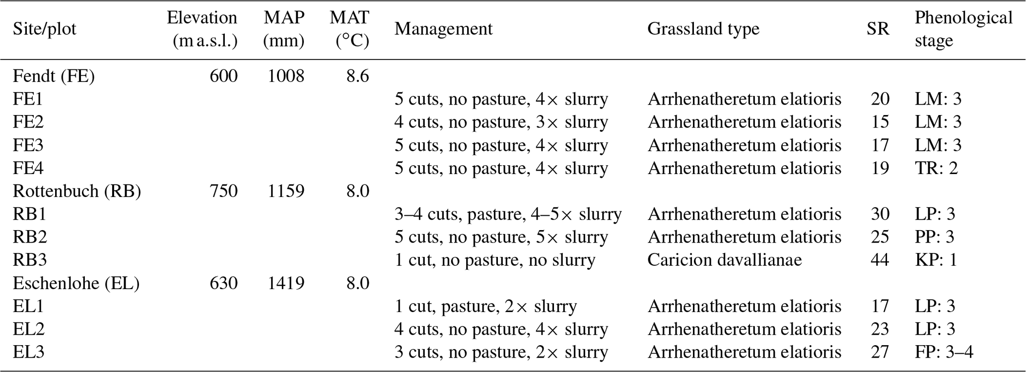
The study area is located in southern Germany (Fig. 1), within the German Terrestrial Environmental Observatories (TERENO) Pre-Alpine Observatory (Kiese et al., 2018; Zacharias et al., 2011). The region is characterized by a warm temperate climate, i.e. Cfb climate zone according to the Köppen–Geiger climate classification (Rubel et al., 2017). For the period 1981–2010 the mean annual air temperature at the study sites was between 8.0 and 8.6 ∘C (DWD Climate Data Center, 2019b), and mean annual precipitation was between 1008 and 1419 mm (DWD Climate Data Center, 2019a). Field data were acquired at 10 plots on managed grasslands (Table 1). The plots are situated on the three sites “Fendt” (FE, 600 m a.s.l.), “Rottenbuch” (RB, 700 m a.s.l.), and “Eschenlohe” (EL, 630 m a.s.l.). Care was taken to include different grassland types and management practices in order to render robust and transferable models also for our single campaign. The plots represent a variety of management intensities ranging from very extensively managed grasslands with no fertilizer application and just one cut per year to very intensively managed grasslands with five cuts and five slurry applications per year. A species inventory in June 2020 characterized 9 out of 10 plots as Arrhenatheretum elatioris, while 1 was classified as Caricion davallianae grasslands (Table 1). Figure 2 provides an overview of the workflow of this study. Details on the different working steps are presented in the following paragraphs and sections.
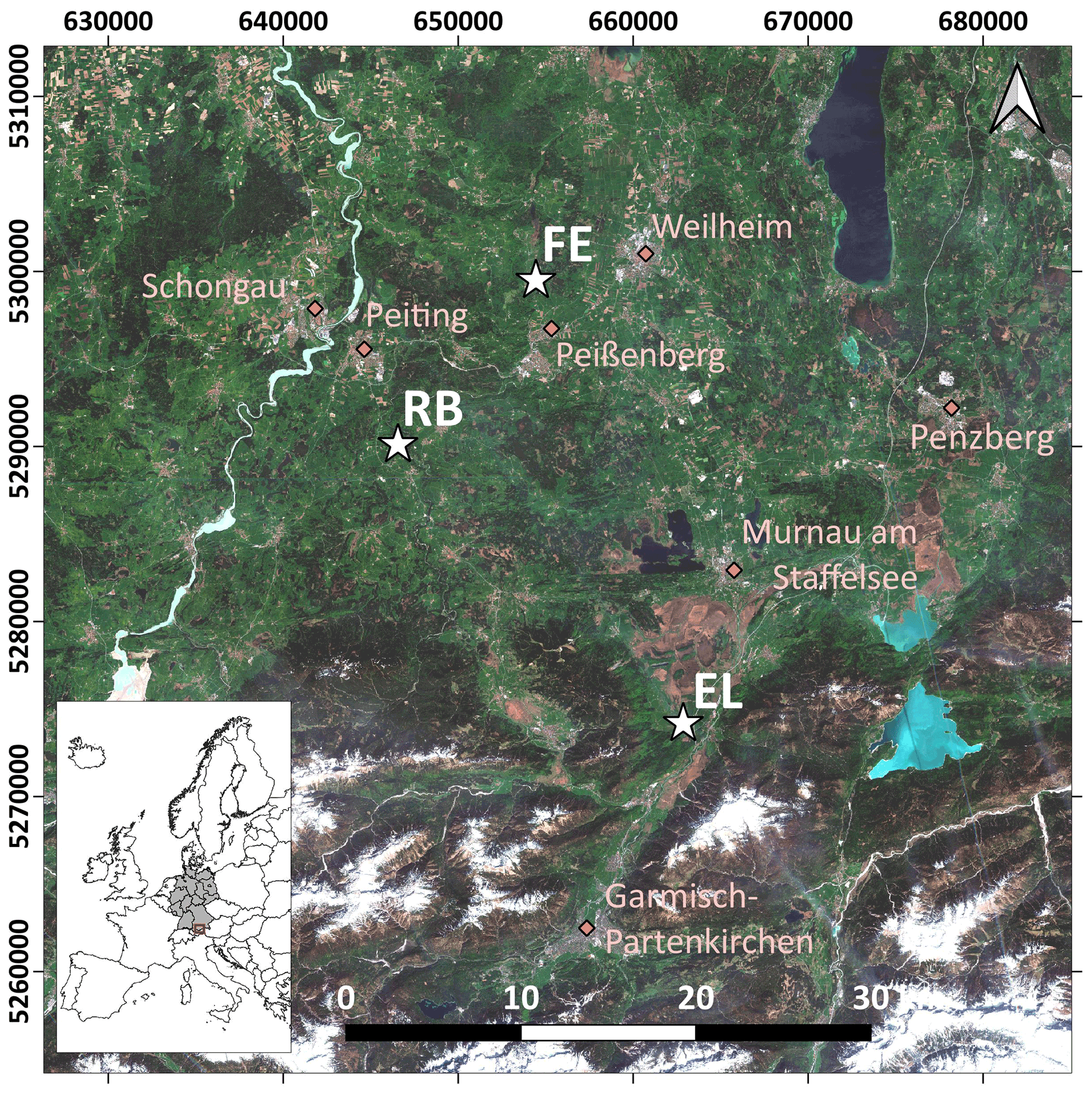
Figure 1Location of the three study sites (white stars) in the study area in the south of Germany. EL: Eschenlohe, FE: Fendt, RB: Rottenbuch. Major towns are indicated for reference (pink diamonds). Background: true-colour composite of Sentinel-2B images from 27 April 2018 (contains modified Copernicus Sentinel data from 2018, processed by ESA). Coordinate reference system used is EPSG:25832.
The field campaign with UAS flights and vegetation sampling took place from 24–25 April 2018. The phenological stage of the plots ranged from principal growth stage 1 (leaf development) to 4 (development of harvestable vegetative plant parts) (Table 1). After the UAS flights, at each site (FE, RB, EL) up to four 30 m × 30 m plots (FE1, FE2, F3, FE4, RB1, RB2, RB3, EL1, EL2, EL3) were sampled at 9 to 12 georeferenced subplots of 0.25 m × 0.25 m. Bulk canopy height (CH, in cm) was measured with a rising plate meter. The vegetation within the subplot was clipped down to stubble height (3 cm). In the lab, the vegetation samples were sorted into the plant functional types of non-green vegetation, legumes, non-leguminous forbs, and graminoids. After the samples were dried in an oven at 65 ∘C until constant weight was achieved, the dry weight was determined, and the dry biomass per area was calculated (dry matter, DM, in g m−2). For the determination of mean plant community nitrogen concentration (plant N concentration, mass-based, in wt %), the dried vegetation samples were milled and analysed with an elemental analyser (vario Max cube, Elementar Analysensysteme GmbH, Germany). The reader is referred to the corresponding data paper (Schucknecht et al., 2020a) for more detailed information on the sampling, sample processing, and analysis.
Table 1Site and plot characteristics partly taken from Schucknecht et al. (2020a). Mean annual climate parameters (MAP: mean annual precipitation height, MAT: mean annual temperature) were derived from the DWD Climate Data Center (DWD Climate Data Center, 2019a, b) and correspond to the period 1981–2010. Grassland type and species richness (SR; i.e. number of vascular plant species) were obtained by a species inventory in 2020 (Schuchardt and Jentsch, 2020). The phenological stage was determined by inspecting the photos of the plots with respect to the dominant species (species abbreviated as LM for Lolium multiflorum, TR for Trifolium repens, LP for Lolium perenne, PP for Poa pratensis, KP for Koeleria pyramidata, and FP for Festuca pratensis). Provided is the number of the principle growth stage (1: leaf development (main shoot), 2: formation of side shoots/tillering, 3: stem elongation or rosette growth/shoot development (main shoot), 4: development of harvestable vegetative plant parts or vegetatively propagated organs/booting (main shoot)) according to the BBCH (Biologische Bundesanstalt für Land- und Forstwirtschaft, Bundessortenamt und Chemische Industrie) classification (Meier, 2018).
From the collected in situ data we used the information from the single subplots to develop the models (see Sect. 2.3). Canopy height (CH) was used as a predictor variable, and DM and plant N concentration were response variables (Fig. 2).
2.2 Acquisition and (pre-)processing of UAS-borne data
2.2.1 UAS flights
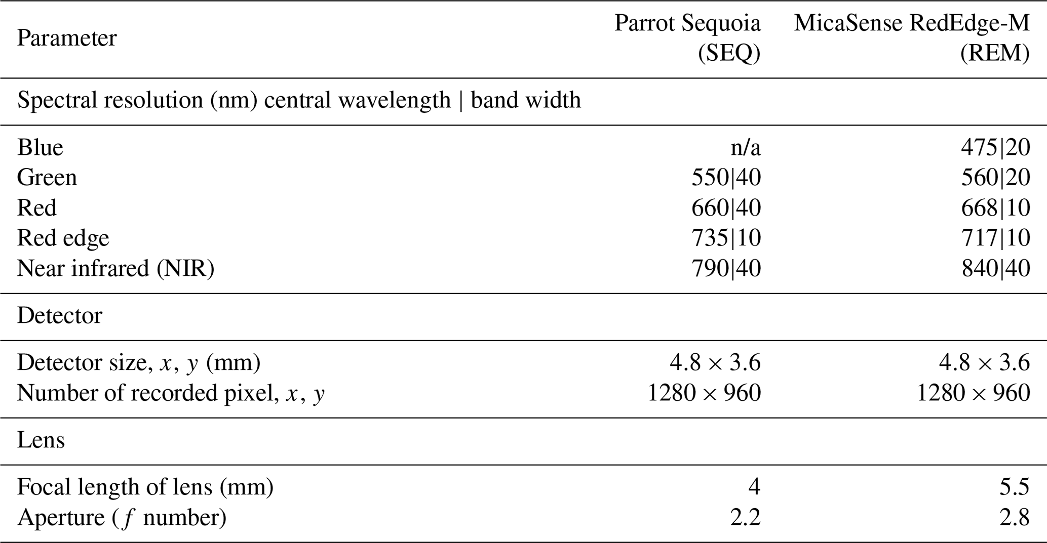
Two different multispectral sensors were tested for this experiment: the four-band Parrot Sequoia (SEQ; Parrot Drones SAS, Paris, France) and the five-band MicaSense RedEdge-M (REM; MicaSense Inc., Seattle, USA) (Table 2). For measuring the incoming solar radiation, both sensors were accompanied by irradiance sensors (“sunshine sensors”) that were attached at the top of the drones. This information was used for image calibration during data processing. Before each flight, data from sensor-specific calibration targets were taken for radiometric calibration of the multispectral images during the processing.
The UAS flights over the FE and RB sites took place on 24 April 2018 between 09:50 and 16:30, and the ones over the EL site (EL-North and EL-South) were on 25 April 2018 between 09:00 and 10:50. The SEQ was operated on a fixed-wing UAS (eBee, senseFly, Cheseaux-sur-Lausanne, Switzerland) with automated flight control. The flight height was set to 80 m, leading to a ground sample distance of 8.7–12.9 cm (depending on the terrain relief). The eBee was flown with a regular grid flight pattern with an image overlap of 75 %.
The REM was operated on a multicopter UAS (DJI Matrice 200, SZ DJI Technology Co., Ltd., Shenzhen, China) by an external company (Globe Flight GmbH, Germany). Due to logistical reasons only the FE and RB sites could be covered. The multicopter was flown manually at a flight height of about 70 m following a regular grid with an overlap of the single images of >80 %. The ground sample distance of the different REM flights was between 7.7–8.8 cm.
For all flights with the different sensors, up to 10 ground control points (GCPs) were distributed in the overflight area of the UAS for georeferencing. The exact coordinates of the GCPs' centres were obtained with a global navigation satellite system (GNSS) receiver (Viva GNSS GS 10, Leica Geosystems AG, Switzerland) run in static mode for 10 min which resulted in an accuracy of 0.3 cm in the horizontal direction and 0.5 cm in the vertical direction in the post-processing mode (Datasheet of Leica Viva GNSS GS10 receiver, 2020).
Table 2Details about the two multispectral sensors used in this study. n/a: not applicable.
2.2.2 Processing of UAS images
The processing of the UAS images was done with the PIX4Dmapper Pro software (Pix4D S.A., Prilly, Switzerland) and consisted of three steps. The photogrammetric processing was based on a structure from motion (SfM) approach. First, keypoints of the images were extracted and matched, and the internal (e.g. focal length) and external (e.g. orientation) parameters of the camera were calibrated. Georeferencing was done with the integration of the measured GCPs and their identification on several input pictures. The root mean square error (RMSE) of the georeferencing varied between 1.9 and 4.7 cm according to the Pix4D processing reports. As a result of the first step, georeferenced automated tie points were created. In the second step, the point cloud densification was done corresponding to the Pix4D standard template for agricultural applications. The final step included the mosaicking of the adjusted and calibrated single images to the orthomosaics of each single band. The final spatial resolution of the multispectral images was 9.6 cm for FE, 10.2 cm for RB-North, 10.0 cm for RB-South, 8.7 cm for EL-North, and 12.9 cm for EL-South for the SEQ data and 7.7 cm for FE, 8.8 cm for RB-North, and 8.2 cm for RB-South for REM data. The radiometric correction of the input images was done using the data of the irradiance sensor and the reflectance panels.
Additional flights of the fixed-wing UAS equipped with an RGB (red–green–blue) camera (Sony Cyber-shot WX 220, Sony Corp., Minato, Japan) were performed on all sites to retrieve higher-resolution orthophotos (spatial resolution: 0.030 to 0.043 m) for the different sites of the study area. The georeferenced high-resolution orthophotos were used to manually extract the coordinates of the centre points of the subplots (Schucknecht et al., 2020a). Afterwards, the reflectance values of the georeferenced multispectral images from SEQ and REM were extracted and averaged for each subplot using a 3 pixel × 3 pixel window around the centre point (Fig. 2, grey box). The 3 pixel × 3 pixel window approximately corresponds to the size of the subplot. Due to the high horizontal accuracy of the GNSS measurements (0.3 cm) and the low RMSE of georeferencing (max 4.7 cm), we expect just minor location errors.
Note that we could just use spectral information from the obtained UAS images as predictors in the model development. Theoretically, it is also possible to derive canopy height information from high-resolution UAS-derived RGB data by creating a digital surface model and subtracting the digital terrain model (DTM) from it as e.g. shown by Grüner et al. (2019) and Wijesingha et al. (2019). Poley and McDermid (2020) emphasized the importance of a high-quality DTM for deriving reliable vegetation structure estimates from UAS imagery. Unfortunately, we did not have such a high-quality DTM for our study sites and hence could not derive UAS-based canopy height information. Therefore, we used the in situ bulk CH as a substitute to build models with CH as a predictor variable.
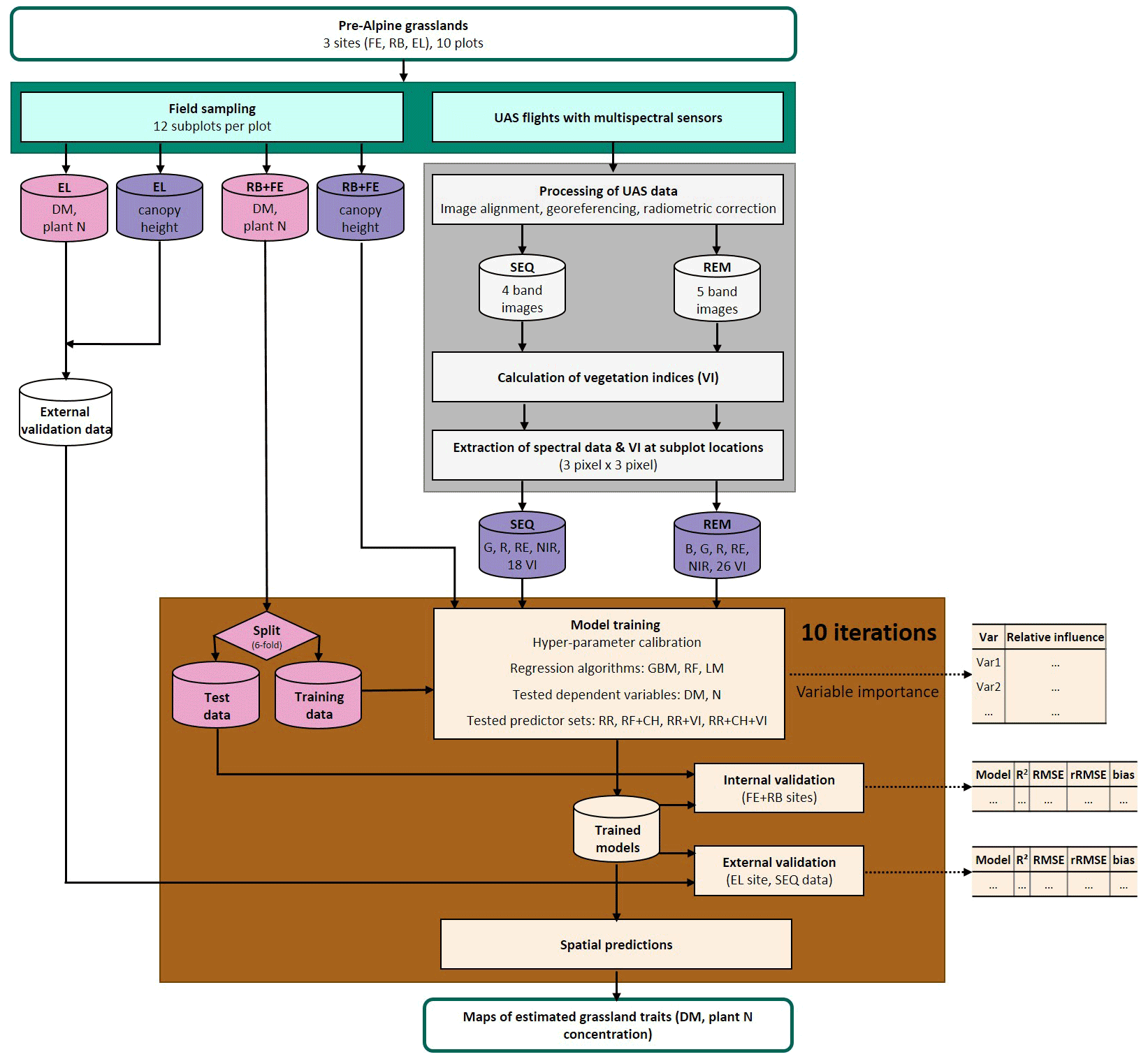
Figure 2Workflow of data acquisition in the field (blue-green); spectral data processing (grey); and model building, validation, and application (brown). Response variables of the model are shown in pink, and predictor variables are in violet. Explanation of abbreviations: sampling sites (FE: Fendt, RB: Rottenbuch, EL: Eschenlohe), predictor variables (B: blue band, G: green band, R: red band, RE: red-edge band, NIR: near-infrared band, VIs: vegetation indices, CH: canopy height), dependent variables (DM: dry matter, N: nitrogen concentration), and regression algorithms (GBM: gradient-boosting machine, RF: random forest, LM: linear model).
2.2.3 Vegetation indices
A set of different vegetation indices (VIs) was calculated from the spectral bands (Supplement Table S1). The various ratio (number of indices used n=6), orthogonal (n=1), hybrid (n=5), red-edge (n=4), and modified chlorophyll (n=4) indices were selected from the overview presented in Asam (2014). In addition, hyperspectral indices dedicated to chlorophyll (n=6) were selected from the summary of Ollinger (2011) and adapted to the multispectral data. In total, 26 VIs were calculated for REM data, and 18 were for SEQ data (due to the missing blue band).
2.3 Model specifications for DM and plant N concentration estimation
2.3.1 Model selection
Regression models were built to estimate DM and plant N concentration based on multispectral UAS data and in situ bulk canopy height information (Fig. 2, brown box corresponding to model building, validation, and application). Combinations of several regression algorithms and predictor sets (PSs) were compared to see how different modelling schemes affect the model performance. Two machine learning (ML) algorithms, namely gradient-boosting machines (GBMs; Friedman, 2002, 2001) and random forests (RFs; Breiman, 2001), were used in this study. They have been confirmed to be comparable to the other state-of-the-art (classic) machine learning methods for remote sensing applications (Caruana and Niculescu-Mizil, 2006; Fernández-Delgado et al., 2019, 2014; Orzechowski et al., 2018). The two selected algorithms are ensemble-based and have a relatively small number of hyper-parameters (Bernard et al., 2009; Friedman, 2001; Probst et al., 2019). These ensemble-based ML algorithms are known to be able to deal with a large number of highly correlated features (e.g. spectral data and derived vegetation indices) and non-linear relationships without excessive data pre-processing (Hengl et al., 2018). In addition to them, a linear regression model (LM) was built to serve as a baseline statistical learning model in the model performance comparison.
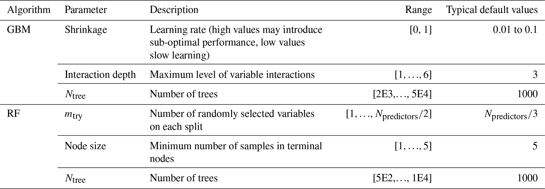
GBM (Friedman, 2002, 2001) is an ensemble of models based on the idea that weak learners can form a strong learner. The algorithm is adding weak models using a gradient descent process. Gradient boosting can take various forms, i.e. different loss functions and optimization schemes. In this study, we took the standard implementation from Friedman (2001, 2002) following Greenwell et al. (2020). GBM has a few tunable parameters, with the major parameters including number of trees (Ntree), learning rate, and interaction depth (see Table 3), which are supposed to be calibrated using domain data to avoid under- and overfitting (Greenwell et al., 2020).
RF is a decision-tree-based ensemble algorithm that uses bootstrap aggregation (i.e. bagging) and the random subspace method (Breiman, 2001). For each decision tree a new bootstrap sample of the training data is created, and the tree is fitted to the data. RF has three hyper-parameters, namely the number of trees (Ntree), the number of randomly selected predictors in each split of the decision tree (mtry), and the minimum number of samples in terminal nodes (node size). It is suggested that for a good model performance the number of trees need to be large enough but should not yield to overfitting (Strobl et al., 2009). The parameter mtry should be carefully calibrated, in particular when predictors are strongly correlated (e.g. Bernard et al., 2009; Kuhn and Johnson, 2013; Probst et al., 2019; Strobl et al., 2009). The node size determines how many samples a tree needs to grow without being pruned.
2.3.2 Hyper-parameter calibration
We parameterized the machine learning algorithms using the nested cross-validation scheme (Arlot and Celisse, 2010; Vabalas et al., 2019; Varma and Simon, 2006) (Table 3). In the nested design, the optimizer in the calibration routine does not see the information included in the hold-out fold. The calibration is done for each of the 10 iterations for randomly split 6 cross-validation folds. For each training fold, parameter searching was done in an internal 5-fold cross-validation using the root mean square error (RMSE) as a penalty function.
To minimize the computing time, we used an efficient parameter space searching algorithm named (sequential) model-based optimization (MBO) (Bischl et al., 2014; Martinez-Cantin et al., 2007; Shahriari et al., 2016). In this algorithm, an optimizer traverses the parameter space guided by a naive Bayesian parameter proposal function, which identifies a candidate region that is likely to include the optimal parameter combinations. In its iterative process, a new parameter proposal is made based on an acquisition function, or “infill”, which is supposed to offer the best improvement in the next step. We used the “confidence bound” as infill for GBM and RF. This infill proposes a parameter combination to minimize uncertainty around the good parameter estimates (Bischl et al., 2014). It tries to evaluate the parameter region with large uncertainty with low errors (i.e. good performance), thus expects to reach a large improvement if searched in the next iteration. In this study, parameter values are proposed and evaluated in 500 iterations sequentially, and the final values are selected by the lowest error. The impact of calibration is quantified by the difference between the initial error (i.e. based on the random combination of the parameters sampled from the prescribed ranges) and the best error, which is defined by the lowest error achieved (Malkomes et al., 2016; Swersky et al., 2013). Note that the calibration was done for the 10 iterations individually; in each iteration the nested six-folds share the calibrated parameters. Calibrated values and their summaries are presented in Table S2 and Figs. S2 and S3.
Table 3Range of the hyper-parameters used in the calibration for gradient-boosting machines (GBMs) and random forests (RFs). The calibration routine searches for the optimal parameter values within the prescribed ranges. Typical default values for the GBM from Greenwell et al. (2020) and RF from Probst et al. (2019). The final calibrated hyper-parameters are presented in Table S2.
2.3.3 Predictor set definition
Six different sets of predictor combinations were used in the models. The number of predictors differs for models using SEQ and REM data and is provided in brackets below:
-
PS1 – raw reflectance bands, using only raw reflectance data from SEQ (n=4) and REM (n=5), baseline scenario
-
PS2 – vegetation indices (VIs), using just VI but not raw reflectance bands (nSEQ=18, nREM=26)
-
PS3 – raw reflectance bands and vegetation indices (VIs) (nSEQ=22, nREM=31)
-
PS4 – bulk canopy height (CH, from field measurements), testing the sole use of CH as a reference for structural information (n=1)
-
PS5 – raw reflectance bands and bulk canopy height (CH, from field measurements), using spectral and structural information (CH) (nSEQ=5, nREM=6)
-
PS6 – raw reflectance bands, CH, and VI, all available spectral and structural input data (nSEQ=23, nREM=32).
Bulk CH was selected as a predictor because we wanted to test the effect of adding structural information; i.e. can the addition of UAS-derived structural information to the spectral information improve the estimation of DM and N concentration in pre-Alpine grasslands? Due to the missing digital CH model for our sites, we used the in situ bulk CH as a substitute. With the in situ bulk CH data we can test the effect of CH on the model results but cannot provide spatial predictions in the form of maps. Hence, models using CH (PS4–PS6) were excluded from spatial predictions.
2.3.4 Input data for model development
We used data from FE and RB plots to train and test (internally validate) the regression models (n=82 for DM; n=81 for N). As REM data were not acquired at the EL site, field data from the EL plots (n=32) were excluded from the model training. However, the field data from the EL plots were used as an additional external validation of the models utilizing data from the SEQ sensor (brown part of Fig. 2; see Sect. 2.3.5).
2.3.5 Model evaluation procedure
To derive robust statistics, the regression models were built using a 6-fold cross-validation and repeated 10 times with random data splits. Each repetition is connoted as an “iteration” throughout the paper. For each iteration, the data are again randomly split into six folds: five folds to train a model and the hold-out fold to test the model. The corresponding cross-validated evaluation metrics are denoted with the subscript “cv”. The model evaluation metrics used in the study are the averages from the test folds of the 10 iterations. Ground observations from the EL site were used to validate the models based on SEQ data without further site-specific training – for this site REM data were unavailable (Fig. 2; corresponding evaluation metrics indexed with the subscript “val”). Evaluation metrics used are the coefficient of determination of the validation (R2), root mean square error (RMSE), relative RMSE (rRMSE), and bias (Bias) (Eqs. 1–4). All metrics were averaged over the 10 iterations.
where y is an observed value, is a prediction, and n is the number of samples. Relative RMSE is normalized by the observed data range and used to compare regression models with unequal data input following Richter et al. (2012).
2.3.6 Model implementation
We used GNU R 3.6 (R Core Team, 2021) for model implementation. GBM was built using the R package “gbm3” (Greenwell et al., 2020), and RF was built via the R package “randomForest” (Breiman, 2001). Linear regression models were built using all available predictors (LMfull) and the best subset of predictors (LMbest) using variable selection. The variable selection was done by an exhaustive search, i.e. evaluate the Akaike information criterion (AIC) (Akaike, 1973) of all possible combinations via the “regsubsets” function in the R package “leaps” (Lumley, 2020). Interactions among the predictors were considered in the ML models but not explicitly in the linear models using interaction terms. We did not include interaction terms in the LMs, as the linear models with (first- and second-order) interaction yielded very large prediction errors in the cross-validation scheme (results from the preliminary analysis, not shown here).
2.3.7 Variable importance
In ML, measuring variable importance (Strobl, 2008) is a standard way to evaluate an overall impact of a specific predictor, often among a large number of highly correlated predictors. In this study, we evaluated variable importance to see how the different predictors overall contribute to the model performance. It is our interest to identify if there is a small number of dominant predictors or rather a combination of many predictors that contain the crucial information. We investigated the variable importance (VarImp) of the predictors used in the ML regression models in each data and model combination.
For each model, we collected variable-importance measures from each 6-fold cross-validation and averaged them; this was repeated for the 10 iterations. As each iteration yielded unequal model performance, the importance metrics of each iteration was normalized by R2 of each iteration before averaging, which resulted in the mean VarImp and its uncertainty range. Note that variable-importance measures are based on reduction in mean squared error (MSE) but calculated differently for each ML algorithm. For GBM, we used the relative influence measure suggested in Friedman (2001) and, for RF, permutation-based out-of-bag importance of Breiman (2001). Various R packages were used to calculate variable importance, depending on the algorithm (Greenwell et al., 2020; Lumley, 2020; Meinshausen, 2017, 2006; R Core Team, 2021).
2.3.8 Mappings: spatial predictions of DM and N concentration
Spatial predictions were calculated for models that do not need CH data (i.e. PS1–PS3). We used the models to predict DM and N values for the whole of the UAS scenes of the three sites. The models are with 10 iterations, thus predicted 10 times, and averages and the coefficient of variations are reported. Note that spatial plant trait estimates may be only valid for pixels of unshaded and vegetated grassland.
2.3.9 Statistical tests for the marginal model performance
Model performance metrics were averaged over sensors, model algorithms, and predictor sets to derive marginal performance with respect to each component. We used non-parametric statistical methods to test the differences in R2 and RMSE. For sensors and algorithms (ntreat=2), we used the non-parametric Wilcoxon signed rank test (Wilcoxon, 1945). For predictor sets (ntreat=4), we used the non-parametric Kruskal–Wallis rank sum test (Kruskal and Wallis, 1952) to test overall effect and Dunn's rank sum test (Dunn, 1964) to carry out post hoc tests between treatments. We used R packages “stats” and “dunn.test” (Dinno, 2017; R Core Team, 2021).
3.1 Variable interdependencies
Correlations between variables measured in the field can affect the modelling of DM and N concentration or can even be exploited to improve the modelling. We created scatterplots of selected variables (Fig. 3) and calculated the Spearman correlation coefficient of canopy height and DM or N concentration, respectively (Fig. 3a, b). Canopy height values varied between 3 and 21 cm (median = 10 cm, n=116) and were significantly correlated with DM (r=0.69, p value < 0.01) but not with N concentration (r=0.02, p value > 0.1). We also found no statistically significant correlation between DM and N concentration (r=0.12, p value > 0.1; Fig. 3c). Based on these results, we would expect that canopy height could improve the modelling of DM but not of N concentration and that any successful modelling of N concentration does not simply reflect a correlation of the spectral data with DM.

Figure 3Scatterplots of field measurements with linear regression line. (a) Canopy height vs. DM. (b) Canopy height vs. plant N concentration. (c) DM vs. plant N concentration. Spearman correlation coefficients and corresponding p values are indicated in the figures. The shaded area corresponds to the standard error bounds of the fitted linear regression line.
3.2 Biophysical and spectral characteristics of field samples
The spectral discrimination of grassland samples with different levels of DM or N concentration is a prerequisite for the estimation of DM and N concentration with multispectral data. In our study, the DM values of the measured subplots varied between 7 and 340 g m−2 (median = 113 g m−2, n=114), and for plant N concentration it was between 1.2 wt % and 4.4 wt % (median = 2.9 wt %, n=113). Despite the fact that we targeted homogenous grassland plots, there was a distinct spatial within-plot variability (Schucknecht et al., 2020a), which however can be reflected by the spatial resolution of the UAS-based multispectral data. In general, the spectral profiles of selected subplots (Fig. 4) follow the expected shape of vegetated surfaces with low reflectance values in the visible range of the spectrum and higher reflectance values in the NIR region. Subplots with different DM and N concentration values show slightly different spectral profiles, with the highest standard deviations of the reflectance values in the red-edge and NIR band. However, the spectral profiles of subplots with different DM or N concentration values do not follow a clear pattern, e.g. with monotonically increasing reflectance of the NIR band with increasing DM. There is a positive linear relationship between NIR reflectance and DM, but this is not very strong (Fig. 5). Additionally, these spectral profiles have altered patterns for the two sensors (Fig. 4), with the SEQ sensor generally showing higher reflectance values (Fig. S1).
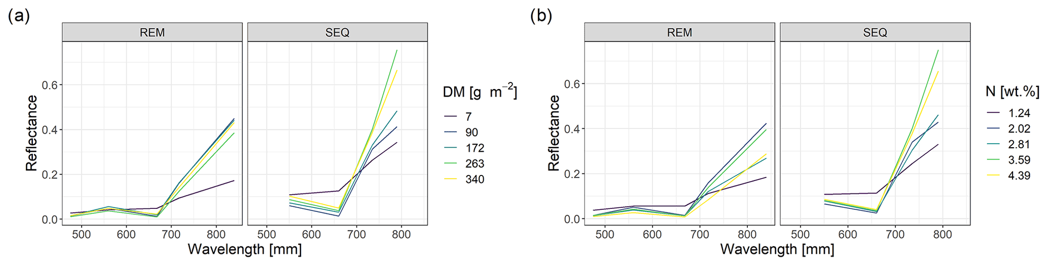
Figure 4Spectral profiles of subplots with different levels of DM (a) and N concentration values (b). Shown are the profiles of the subplot samples with min and max values as well as the ones that have DM or N concentration values that approximately correspond to the 25th, 50th, and 75th percentile.
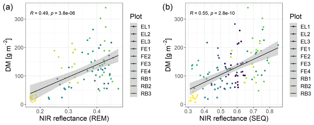
Figure 5Scatterplots of NIR reflectance vs. DM with linear model fit (Spearman correlation coefficient and p value indicated in the plot) (a) for REM sensor and (b) for SEQ sensor. Note: there are fewer data points for REM, as there were no flights with this sensor at the Eschenlohe site.
3.3 Hyper-parameter calibration
During the calibration process, the model performance increased, as improved parameter sets are used in the course of the iteration procedure (Fig. S2). Compared to initial model performance, which is based on 12 randomly sampled parameter sets from the given ranges (i.e. first 12 time steps in calibration; Bischl et al., 2014), the magnitude of improvement on average was 11 %. The difference between the lowest error achieved and the initial error is 19.4 % (GBM) and 5.5 % (RF) in DM estimation and 16.1 % (GBM) and 2.9 % (RF) in N concentration estimation, averaged for the REM and SEQ sensor. Thereby the best error (i.e. the smallest error achieved by the ith iteration) did not substantially decrease as the optimizer approaches the global optimum after 400 iterations in most of the cases (Fig. S2). However, in some cases better parameter values were still discovered at the very end of the iteration procedure (e.g. PS1 in Fig. S1a). RF parameters changed less than GBM parameters along the iterations (Fig. S1b and d). Furthermore, parameter proposals are less fluctuating for RF than for GBM as shown in the distance between consecutive parameter proposals (Fig. S3).
3.4 Model results
Our results indicate that the ML algorithms performed substantially better than the linear models in estimating DM and plant N concentration (Tables 4, 5, S3). ML algorithms yield an average regression performance of 0.44 for . Throughout the sensor–predictor set combinations, average (avg) was 0.48 for DM (rRMSEcv,avg=15.9 %; Table 4) and 0.40 for plant N concentration (rRMSEcv,avg= 15.2 %; Table 5). In contrast, the “baseline” linear models are very low in , seemingly unsuitable to estimate DM and plant N concentration (all models ; Table S3). Therefore, we focus in the following on the detailed results from the ML models (Figs. 5, 6; Tables 4, 5) and further investigate their characteristics.
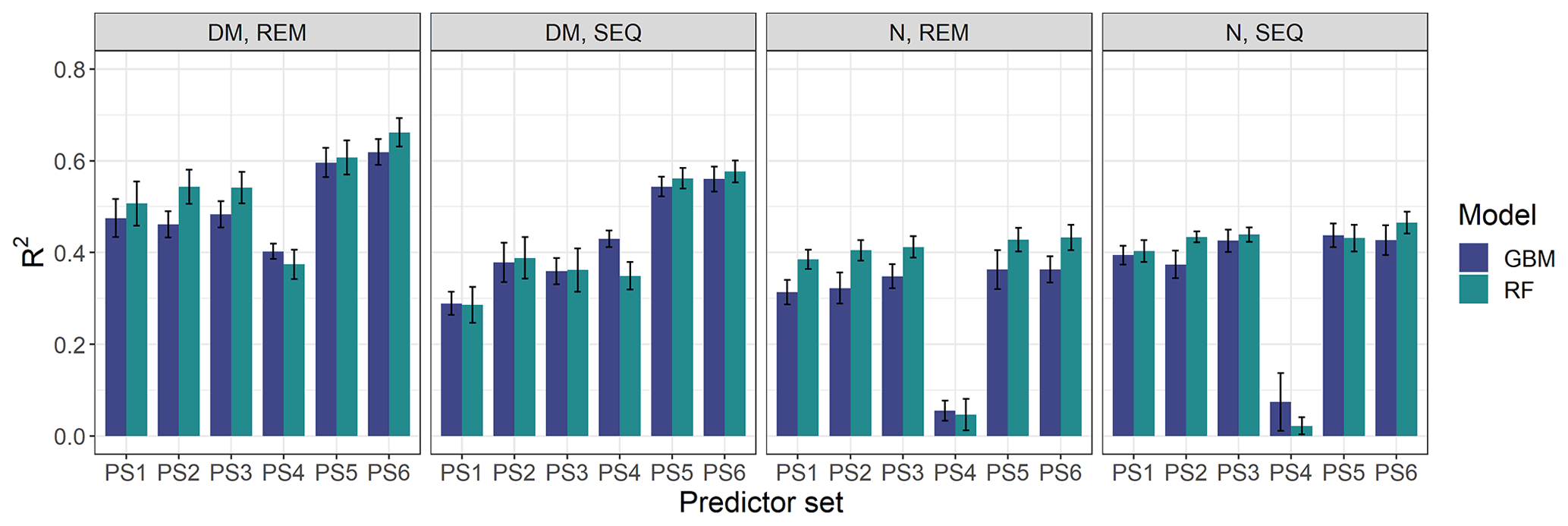
Figure 6Overview of modelling results for all tested combinations of parameters (DM, plant N concentration), sensors (REM, SEQ), ML algorithms (GBM, RF), and predictor sets (PS1: raw reflectance data, PS2: VI, PS3: raw reflectance data + VI, PS4: canopy height, PS5: raw reflectance data + canopy height, PS6: raw reflectance data + VI + canopy height). The bars show the mean of the cross-validated coefficient of determination (R2), and the error bars represent ± standard deviation of the 10 iterations per model.
The optimal combination of sensors, predictor sets, and ML algorithms leads to a notable increase in model performance compared to the average performance of all ML models – for both DM and plant N concentration (Tables 4, 5; Fig. 5). The best model for the estimation of DM (, rRMSEcv=12.6 %) is an RF model that utilizes all possible predictors (PS6) with REM sensor data (Fig. 6a). The best model for plant N concentration (, rRMSEcv=14.2 %) is achieved by the combination of RF, the PS6 predictor set, and SEQ input data (Fig. 6d).
The bias of our tested ML models varies between −2.5 and 2.2 g m−2 for DM (Biascv,avg=0.1 g m−2) and between −0.04 wt % and 0.01 wt % for N concentration (Biascv,avg=0.00 wt %). Although overall biases are low (Bias % of the mean DM and mean N observation), the models tend to underestimate high DM and high N plant concentration (Figs. 6, S7, and S8).
3.4.1 Effect of different sensors
The effect of the multispectral sensor on the model performance varied by the different grassland parameters. For DM, the models that built on REM input data perform better (R2cv,avg=0.52, RMSEcv=50.6 g m−2) than models that built on SEQ data (, RMSEcv=57.5 g m−2) averaged over algorithms and predictor sets (Table 4). This difference is statistically significant for and RMSEcv (p value < 0.01; Fig. S4a, c). Additionally, we tested the models built on REM data without the blue band to see if the performance gap is due to the additional blue band of REM. The results show generally better performance of the REM-without-blue-band-based models (R2cv,avg=0.54) than SEQ-based models (Table S3), suggesting that the better performance of models using REM data is not (entirely) related to the additional blue band.
Considering the estimation of plant N concentration (Table 5), models utilizing SEQ input data perform generally better (R2cv,avg=0.43, RMSEcv=0.50 wt %) than those using REM input data (R2cv,avg=0.32, RMSEcv=0.52 wt %), and these differences are statistically significant for but not for RMSEcv (p value < 0.01 for , p value = 0.092 for RMSEcv; Fig. S4b, d).
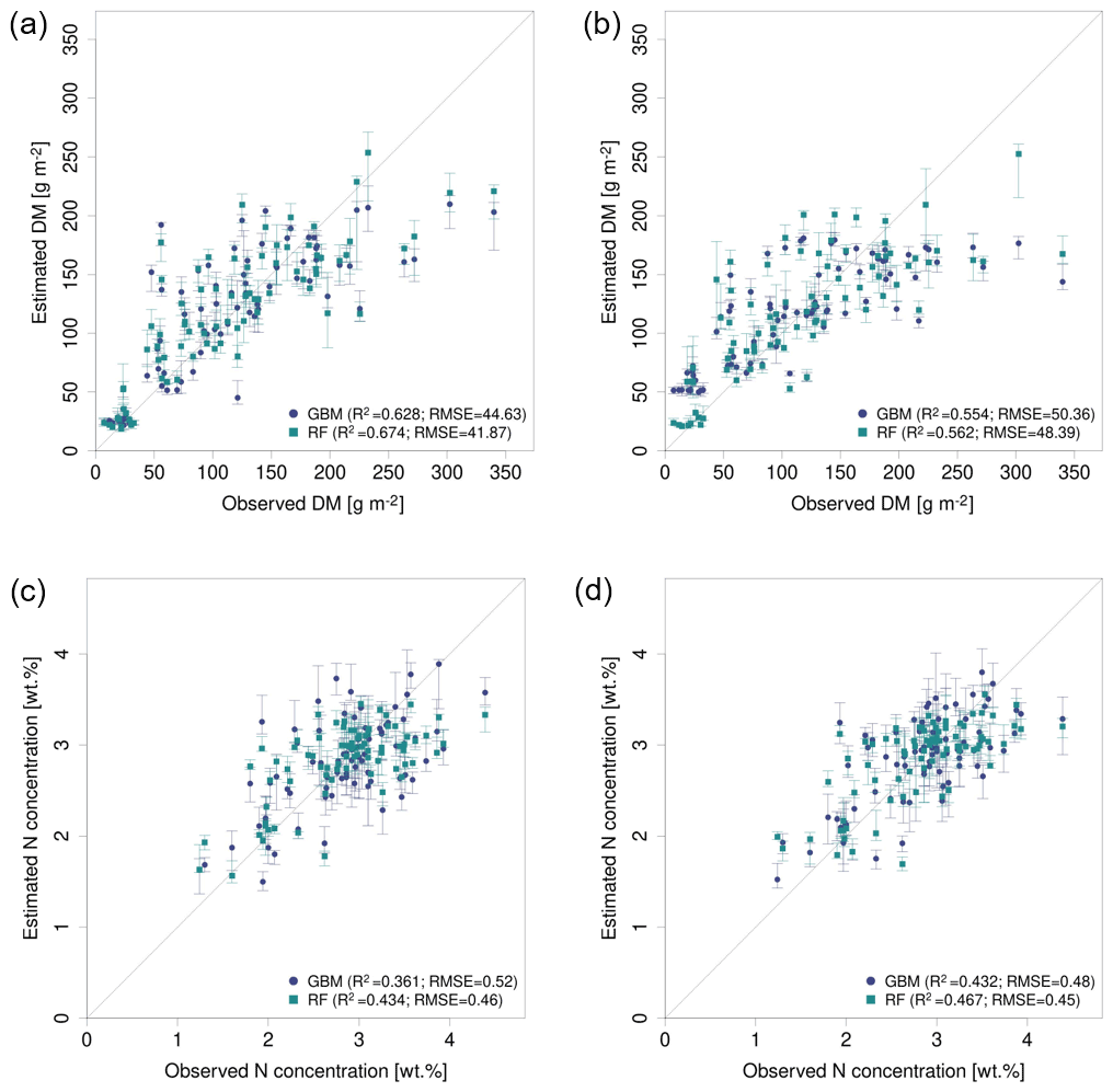
Figure 7Observed vs. estimated parameter values for the best performing predictor set PS6 (raw reflectance data + VI + canopy height) comparing GBM and RF models (a) for DM with REM data, (b) for DM with SEQ data, (c) for N concentration with REM data, and (d) for N concentration with SEQ data. The error bars reflect 90 % prediction intervals, defined by 5th and 95th percentiles of the 10 iterations.
Table 4Overview of the DM models and cross-validation evaluation metrics for all combinations of sensors (REM, SEQ), predictor sets (PS1: raw reflectance data, PS2: VI, PS3: raw reflectance data + VI, PS4: canopy height, PS5: raw reflectance data + canopy height, PS6: raw reflectance data + VI + canopy height), and ML algorithms (GBM, RF). The unit of RMSEcv and absolute Biascv is grams per square metre. All metric values of single-sensor–predictor set–algorithm combinations are averages of the 10 iterations. Best results per sensor in bold. The first 11 rows per parameter show aggregated median results (e.g. median of all DM models). Nobs=82.
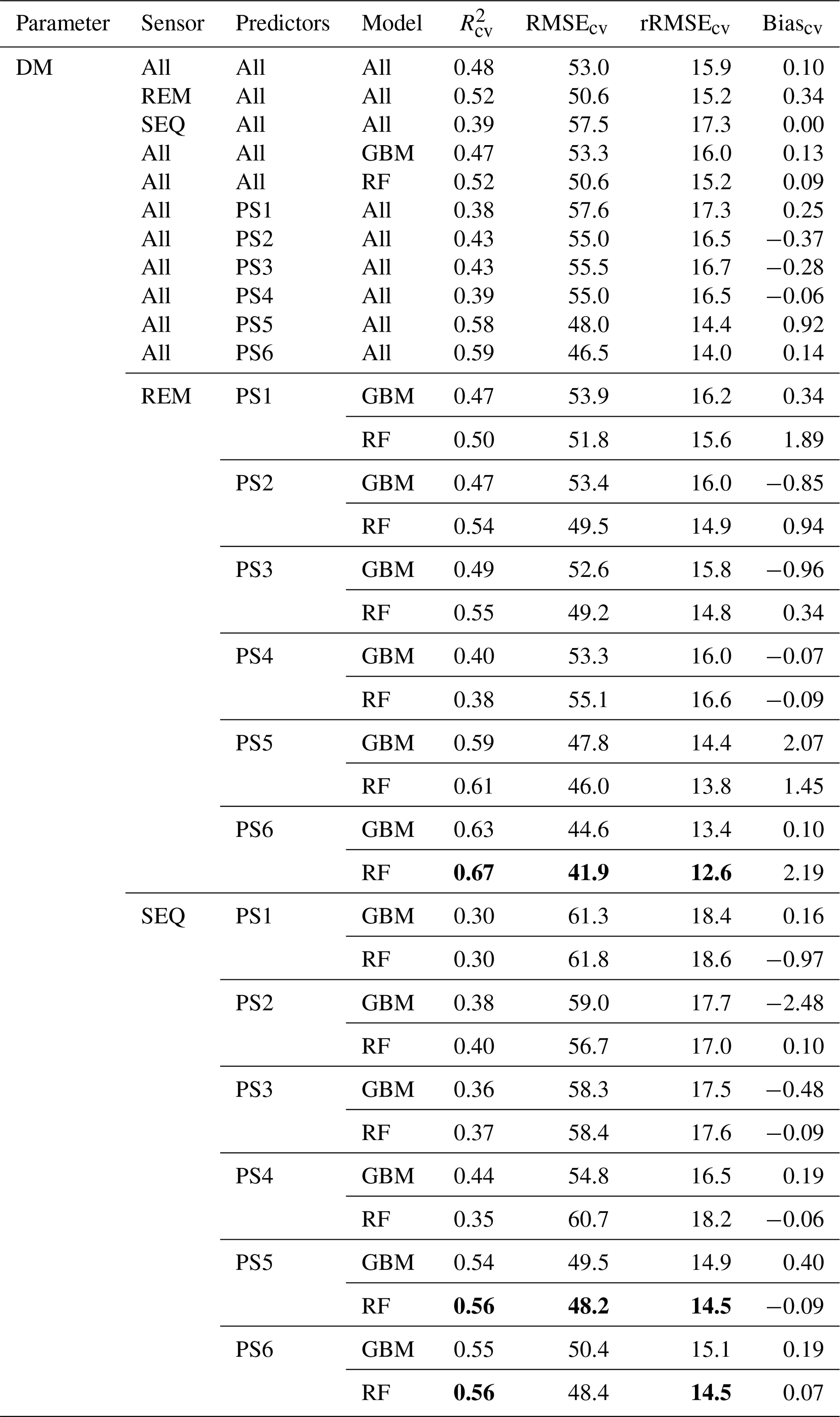
Table 5Overview of the plant N concentration models and cross-validation evaluation metrics for all combinations of sensors (REM, SEQ), predictor sets (PS1: raw reflectance data, PS2: VI, PS3: raw reflectance data + VI, PS4: canopy height, PS5: raw reflectance data + canopy height, PS6: raw reflectance data + VI + canopy height), and ML algorithms (GBM, RF). The unit of RMSEcv and absolute Biascv is weight percent. All metric values of single-sensor–predictor set–algorithm combinations are averages of the 10 iterations. Best results per sensor in bold. The first 11 rows per parameter show aggregated median results (e.g. median of all DM models). Nobs=81.

3.4.2 Effect of predictor sets and variable importance
The selection of the subsets of predictors clearly influences the performance of DM models (Figs. 5, S6, S7; Tables 4, A1). For REM-based models, all predictor sets that only use spectral data (i.e. PS1: raw reflectance; PS2: VI; PS3: raw reflectance + VI) show a similar and slightly higher performance than the predictor set using only canopy height (PS4). For SEQ-based models, the use of VI (PS2, PS3) or canopy height only (PS4) improves the model performance compared to the baseline scenario just using raw reflectance data (PS1). The best model results for REM- and SEQ-based models are obtained by combining spectral data with canopy height information (PS5, PS6). These predictor sets show significantly higher and lower RMSEcv than predictor sets with spectral data (PS1, PS2, PS3) or canopy height information only (PS4).
For plant N concentration (Figs. 6, S6, S8; Table A1), the models using spectral predictors (PS1, PS2, PS3) show a similar model performance (R2cv,avg=0.39–0.42) that is insignificantly lower than for models using all available predictors (PS6; R2cv,avg=0.43). Models using just canopy height as the predictor are not capable of predicting N concentration (R2cv,avg=0.04) and perform notably worse than all other predictor sets (p value < 0.05 for RMSEcv; p value < 0.05 for except for the comparison of PS1 and PS4).
Variable importance
The analysis of variable importance shows some general observations (see Table S4 for detailed results). The added value of the inclusion of structural information in the predictor set for the estimation of DM is further substantiated by canopy height having the highest relative variable importance in all predictor sets where it is included (PS5, PS6), independent of the used sensor data and ML algorithm. For example, canopy height accounts on average for 39 % of error reduction, measured by relative importance for all models using PS5, and 28 % for the all models using PS6. Besides, the NIR band shows the highest variable importance for DM estimation (Table S4) over all sensor–algorithm combinations in the baseline scenario (PS1). For predictor set PS5 (raw reflectance + CH), the NIR band has the second highest variable importance after canopy height, again over all sensor–algorithm combinations. If VI and raw reflectance were included in the predictor set (PS3, PS6), one (PS3 with the SEQ–GBM combination) or a few VIs (all other sensor–algorithm combinations) are ranked higher than the raw reflectance band with the highest variable importance. Vegetation indices that have a variable importance of at least 5 % in all sensor–algorithm combinations of predictor sets including VI (PS2, PS3, PS4) are the Datt's index (Datt, 1999), NDVIre, and RR1, which all include the NIR band in their formula (Table S1).
In contrast to DM, there is in general no clear order or dominance of a certain predictor recognizable over all sensor–algorithm combinations for the estimation of N concentration. Canopy height shows a much lower variable importance compared to the DM models, with average relative importance of 15 % for PS5 and 8 % for PS6.
3.4.3 Effect of modelling algorithm
Overall, the two tested ML algorithms show a smaller difference in model performance than the two sensors and the predictor sets (Tables 4, 5; Fig. S5) for DM and plant N concentration. RF usually performs better (DM: R2cv,avg=0.52; N: R2cv,avg=0.42) than GBM (DM: R2cv,avg=0.47; N: R2cv,avg=0.36), but neither the difference in and RMSEcv between GBM and RF for DM nor the difference in RMSEcv for N concentration is significant (p value > 0.1). Models using REM data generally show a higher difference in model performance between GBM and RF, both when considering DM and N.
Noticeable is the distribution of relative importance of the predictors between the two ML algorithms (Table S4). GBM is often characterized by one dominating variable (especially for DM), which has substantially higher relative importance than other variables. In contrast, RF models show a more gradual decrease in variable importance for the subsequent ranked predictors.
3.4.4 External model validation with data from Eschenlohe (EL)
The models based on SEQ sensor data were additionally validated against the ground observations from the EL site that were not used for model training. Considering DM models (Table 6), the validation results for the EL plots show lower R2 and higher RMSE values compared with the cross-validated model results of the RB and FE sites (Table 4). Furthermore, the model predictions for EL are more biased (Bias g m−2). As seen in the cross-validated results, particularly high DM values are generally not well captured with a clear downward bias (Figs. 7, S9). The best model for the estimation of DM in EL (, RMSEval=41.0 g m−2, rRMSEval=18.4 %) uses RF with predictor set PS6 (raw reflectance data + VI + canopy height). Prediction of DM for EL is significantly improved by the use/inclusion of canopy height as predictor (PS4, PS5) and to a lesser extent by VI (PS2, PS3) (Table 6, Fig. S9).
All N concentration models show very low R2 values () for the external validation site (Table 6). The models for the external validation site predict levels of N concentration >2.2 wt % but do not sufficiently capture the variations between 2.2 wt % and 4.1 wt % (Figs. 8b, S10). The GBM model using PS4 (canopy height) predicts a single value for all N observations (Fig. 8b), implying that the model is not sensitive in this range. The levels of rRMSE (rRMSEval,avg=28.0 %) are also higher than those of the cross-validated results (rRMSEcv,avg=16.3 %).
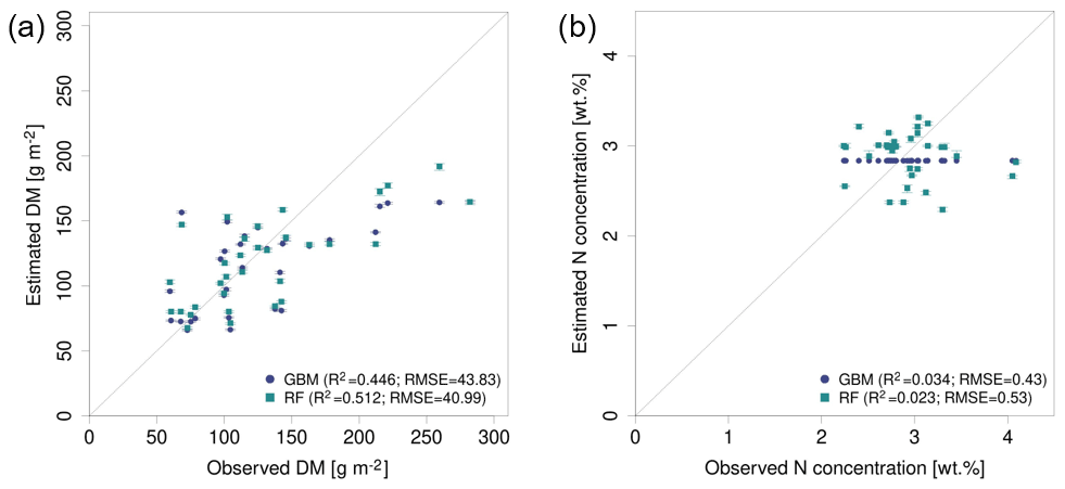
Figure 8Observed vs. estimated DM (left) and N concentration (right) in the external site EL using SEQ data with the best performing predictor set: (a) DM models based on PS6 (raw reflectance data + VI + canopy height) and (b) N concentration models based on PS4 (canopy height).
3.5 Spatial predictions
The spatial DM prediction with the best performing spatial model (RF model with REM data and predictor set PS3 – raw reflectance data + VI) for the RB-North site shows within-field variability (Fig. 9a). Furthermore, the extensively managed field around plot RB3 is characterized by very low DM values, which corresponds to field observations. The individual iterations of this model combination show very similar DM predictions that just differ slightly in areas with low DM as indicated by the coefficient of variation (CV) of the 10 iterations (Fig. 9b). Compared to this, the difference in spatial DM prediction between different DM model combinations (Fig. 9c) is much higher with the highest differences (CV > 30 %) occurring at places with very low DM. The main spatial pattern between different model combinations is similar, but less pronounced spatial patterns may differ depending on the used combination of sensor, ML algorithm, and predictor set.
The spatial prediction of plant N concentration for the RB-North site (Fig. 9e) also shows a certain within-field variability, and the extensively managed field around plot RB3 stands out with very low N concentrations. Most of the grassland pixels outside the extensive field are characterized by N concentrations between 2.5 wt % and 3.5 wt %. The differences between the 10 iterations of one model combination (Fig. 9e) and between different model combinations (Fig. 9g) are generally lower than for the DM models.
The spatial prediction maps for the other sites (Figs. S11 to S14) also indicate within-field and between-field variability in DM and plant N concentration as well as the highest differences between models at grassland areas with low values of DM and N concentration.
Table 6External model validation with the EL site using SEQ sensor data. The unit of RMSEval and Biasval of DM is grams per square metre, and it is percent weight for plant N concentration. Shown are all combinations of predictor sets (PS1: raw reflectance data, PS2: VI, PS3: raw reflectance data + VI, PS4: canopy height, PS5: raw reflectance data + canopy height, PS6: raw reflectance data + VI + canopy height), and ML algorithms (GBM, RF). All metric values of single-sensor–predictor set–algorithm combinations are averages of the 10 iterations. Best results in bold. The first nine rows per parameter show aggregated median results (e.g. median of all DM models). Nobs=32.
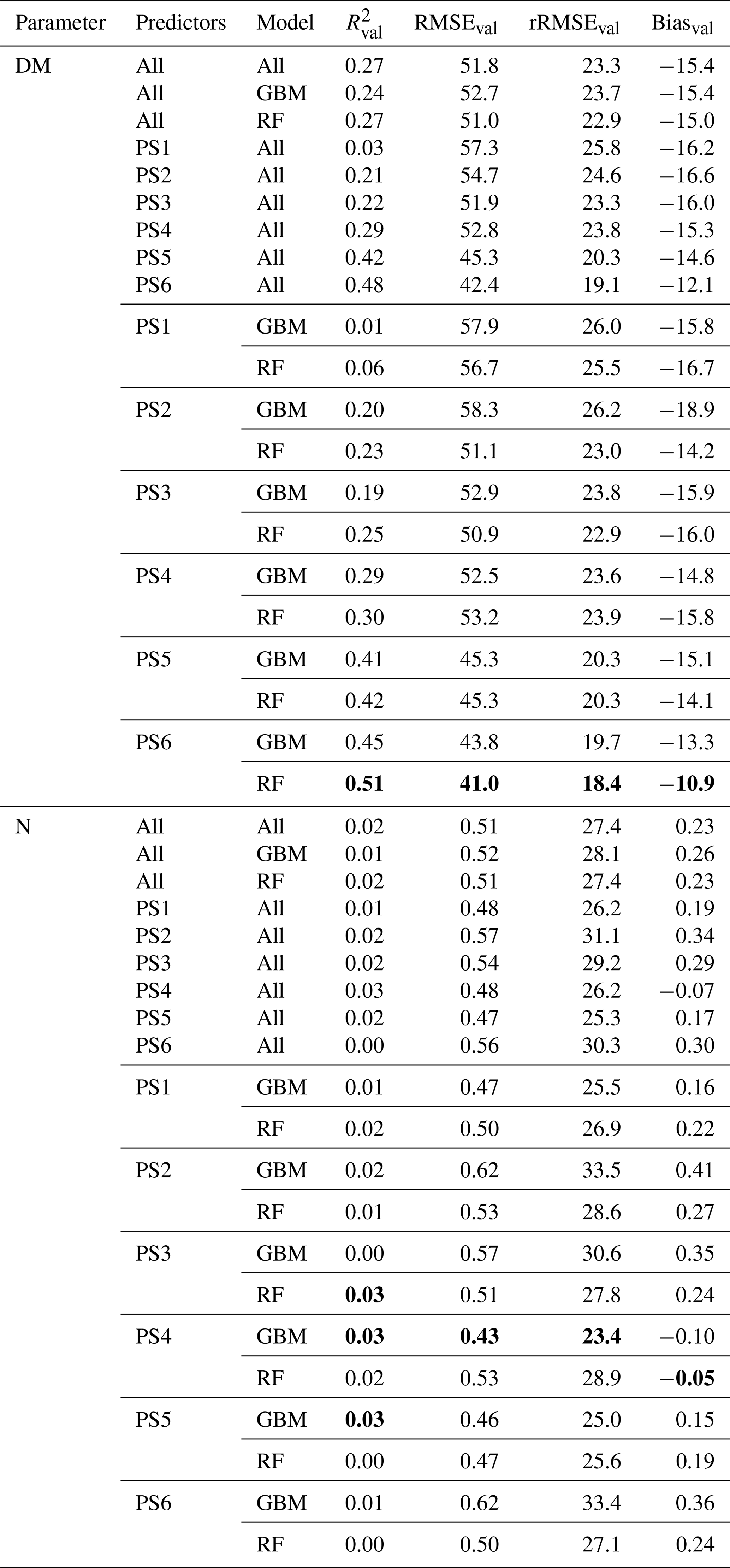
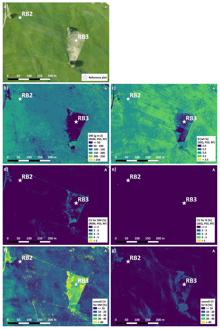
Figure 9Spatial estimation at the RB-North site. (a) Orthophoto for comparison. (b) DM with an REM–PS3–RF combination (best spatial prediction). (c) N concentration with an SEQ–PS3–RF combination (best spatial prediction). (d) CV of DM with an REM–PS3–RF combination. (e) CV of N concentration with an SEQ–PS3–RF combination. (f) Overall CV of DM for all PS1 and PS3 models. (g) Overall CV of N concentration for all PS1 and PS3 models. Predictor set PS3: raw reflectance data + VI. Estimation of DM and N concentration represents the mean of the 10 iterations for the selected model. Note that spatial estimates are only valid for pixels of unshaded and vegetated grassland.
In this study, we analysed the potential to estimate DM and plant N concentration with low-cost UAS-based data in pre-Alpine managed grasslands. We tested two multispectral sensors, three statistical models, and six different predictor sets and evaluated marginal effects of them. The models were trained and validated with in situ data. An emphasis was put on the calibration of the two ML algorithms GBM and RF.
4.1 Suitability of multispectral data to estimate DM and plant N concentration
The spectral differences between samples of different DM and plant N concentration levels (Fig. 4) indicate that an estimation of these two grasslands parameters could be obtained by multispectral UAS data. However, the link between spectral pattern and the level of DM or plant N concentration, respectively, does not seem to be straightforward as e.g. demonstrated by the weak linear correlation between DM and NIR reflectance and the unsuitability of linear models to estimate DM and plant N concentration. Potential reasons for the rather weak bivariate relationship could be the different species compositions of the subplots, differences during the acquisition (time during the day, clouds), and the radiometric correction of the multispectral sensors (see Sect. 4.7 for a more detailed discussion of UAS acquisition issues), which can be challenging and a source of uncertainty (Olsson et al., 2021). Accordingly, our model results confirmed that the estimation of DM and plant N concentration is feasible when applying machine learning algorithms but with a noticeable error range. The best models using all available multispectral data (i.e. raw reflectance and VI) plus bulk canopy height information achieved an of 0.67 (rRMSEcv=12.6 %) for DM and an of 0.47 (rRMSEcv=14.2 %) for N concentration. These findings are in line with other studies which also confirmed the suitability of ML algorithms for grassland parameter estimation based on UAS data. The multitemporal study of Grüner et al. (2020) of an experimental farm with legume–grass mixtures also applied an RF model to the spectral-reflectance data and VI of an SEQ sensor and achieved an of 0.62 and rRMSEcv of 17 % for DM estimation. The authors showed that the modelling performance was clearly improved by adding texture parameters to the predictor set ( and rRMSEcv of 11 %). The analyses of Wijesingha et al. (2020) addressed the prediction of forage quality in grasslands with multitemporal hyperspectral UAS data in the wavelength range between 450–998 mm. They compared different regression algorithms and found that support vector regression worked best for the prediction of crude protein (, cross-validated normalized RMSEcv=9.6 %), but RF yielded similarly good results.
In our study, plant N concentrations models did not perform as well as the DM models, generally achieving much lower accuracies. The same decrease in accuracy was also found for the external validation site, where the N models marked much lower R2 and higher RMSE values compared to the DM models. Furthermore, the N concentration models benefitted to a much lesser extent from the addition of the canopy height information to the spectral predictors. One reason for the less good performance of N concentration models in our study is certainly the result of the lower value range of plant N concentration (coefficient of variation in all samples, CV %) compared with DM (CVDM,all=57.3 %). Most of the N concentration in leaves is related to pigments like chlorophyll and proteins involved in photosynthesis with the most important being Rubisco (Ollinger, 2011, and references therein). While pigments are the dominant absorbers in the visible range of the electromagnetic spectrum, non-pigment compounds mainly have absorption features at longer wavelengths (Ollinger, 2011, and references therein). In his review, Ollinger (2011) summarizes several hyperspectral vegetation indices that are used for chlorophyll detection. However, the author emphasized that the effects of plant N concentration on leaf spectra are still unclear, e.g. if spectral reflectance is mainly driven by direct effects of N-containing compounds or indirect effects of related traits. In a recent publication, Berger et al. (2020) question the use of the commonly used chlorophyll–nitrogen relationship, as it is not maintained after the vegetative growth stage, and propose to quantify instead leaf protein concentration. The authors recommend the use of hyperspectral sensors for N quantification, as the spectral signatures related to proteins are subtle and mainly located in the short-wave infrared (SWIR) region. This should be further explored together with ML models trained on radiative transfer models (Berger et al., 2020) or other modelling approaches like crop, plant growth, or biogeochemical models assimilating remote sensing data.
4.2 Importance of machine learning algorithms and their calibration
Linear models generally failed to capture variability both in DM and plant N concentration estimation as expressed in the cross-validated predictive performance. In all cases, the predictive performance was substantially better for ML algorithms. Linear models do not cope well with a large number of highly correlated predictors as well as with non-linearity (Marchese Robinson et al., 2017). Explorative modelling techniques such as manual feature engineering in linear models, including advanced models such as generalized linear models, may help to achieve better model performance to the level of ML algorithms, as those methods can cover some weaknesses of LM.
As shown in the results, hyper-parameter calibration of ML algorithm was confirmed to be crucial, leading to 11 % improvement in model performance. The lowest error was not revealed in the early iterations, and the parameter searching was discovering lower error values almost until the end of the iterations, suggesting that there is a risk of drawing inference based on the sub-optimal result when “default” parameter values are used. Note that the impact of calibration was more pronounced for GBM; in contrast the calibration of RF was seemingly more efficient (i.e. discovered optimal parameter values in a smaller number of iterations) in line with previous studies (Bernard et al., 2009; Probst et al., 2019). The MBO algorithm used in the calibration is more efficient in exploring a high-dimensional parameter space than naive searching algorithms such as grid searching, random sampling, or Latin hypercube sampling (Bischl et al., 2014). MBO does not need binning or discretization and can also stop earlier than scheduled, unlike grid searching, when it reaches the prescribed goal or yields no improvement. Those features enable MBO to explore parameter domains more comprehensively and effectively. A caveat of the adaptive algorithm is that it needs prescribed stopping rules (e.g. number of iterations or percent of improvement), though such stopping rules do not assure the optimal performance. Objective stopping rules should be further investigated in future applications such as metrics based on convergence, e.g. the Gelman–Rubin diagnostic commonly used in Markov chain Monte Carlo modelling (Brooks and Gelman, 1998; Gelman and Rubin, 1992).
In this study, a nested cross-validation scheme is applied ensuring that the calibration routine does not see the hold-out data. Otherwise, the calibration could rather lead to loss of predictive power (Vabalas et al., 2019). We should note that the DM and plant N concentration values of the validation site (EL) are within the range of observations made in the training sites (Schucknecht et al., 2020a). Training data spanning a wide range of observed DM and N concentration values and maybe originating from different types of grassland at different times in the growing season would be desired to build a generally applicable model. Overall, the two tested ML algorithms yielded comparable model performance after calibration; RF performed slightly better (higher and lower RMSEcv) but without statistical significance.
4.3 Impact of different sensors
The two tested multispectral sensors affected the model performance in different ways depending on the considered grassland parameter. While REM-based models outperformed SEQ-based models in the estimation of DM, SEQ-based models yielded significantly better results for plant N concentration estimation in terms of and RMSEcv. The two sensors have a different spectral setup with slightly different central wavelengths. While SEQ has a wider green and red band, REM has an additional blue band. Furthermore, the red-edge bands of the two sensors are not overlapping as well as the NIR bands. Considering some reflectance spectra of grass (e.g. USGS spectral characteristics viewer, https://landsat.usgs.gov/spectral-characteristics-viewer (last access: 12 May 2022); Rossi et al., 2020; Rossini et al., 2012), we would assume that the difference in the red-edge band position could lead to significant reflectance differences between SEQ and REM for one sample (due to the steep increase in reflectance in the red-edge region). The effect of the different central wavelength in the NIR band might be less pronounced (as the NIR plateau is reached), and the different band width of the green and red bands are expected to have a negligible effect on the difference in reflectance value between the two sensors. These and other constructional differences in the sensors might partly explain differences in the spectral profiles of certain subplots (Fig. 4) and thus differences in model performance.
A possible reason for the SEQ sensor showing generally higher reflectance values than the REM sensor with sometimes even implausibly high reflectance values in the NIR band (>0.7; Figs. 5, S1) might be calibration issues of the sensor. The radiometric correction of the multispectral sensors, which is needed to convert digital numbers to surface reflectance, can be challenging and a source of uncertainty (Olsson et al., 2021), which might be even more important than the spectral specification of the sensors. Poncet et al. (2019) compared different radiometric correction methods for the Parrot Sequoia sensor including the manufacturer method using a one-point calibration plus a sunshine sensor like in our study. The authors found no method allowing for maximizing data accuracy for all bands and different flight conditions. The manufacturer-recommended method that includes the sunshine sensor yielded comparable data accuracy as the best empirical method but could be improved by the combination with an empirical calibration (Poncet et al., 2019). In their study, Olsson et al. (2021) evaluated the accuracy of the Parrot Sequoia camera and sunshine sensor, highlighting the influence of the camera temperature on the sensitivity of the camera, the influence of the atmosphere on the images, and the influence of the orientation of the sunshine sensor on raw irradiance data. We were not aware that the Sequoia sensor needs to be sufficiently warm before reaching a stable sensitivity (Olsson et al., 2021). Since we took images of the sensor-specific calibration targets before each flight, this might have negatively influenced our radiometric calibration and introduced uncertainty in the reflectance data. The above-mentioned difference between the reflectance levels measured by the two sensors is not likely to have a considerable effect on the results of the estimation of canopy traits, as only data from one of the sensors are used in model fitting. However, this means that the results from the model fit will only be valid for the reflectance data from the sensor used, and parameters from different model fits based on data from the two sensors are thus not directly comparable. Proper calibration of the two sensors would therefore be advised in future studies to make the results more generally applicable and comparable.
Besides constructional and radiometric correction aspects, changing illumination conditions may have contributed to differences in the reflectance values of a certain subplot in the comparison of the two sensors. Data acquisition at the Fendt site was partly affected by passing clouds, which is also visible in the data of the irradiance sensor of the SEQ (not shown). In general, it would be beneficial to have in situ reflectance data of the subplots (e.g. from a field spectroradiometer) to validate the reflectance values of the two UAS sensors, but these are not available.
In summary, we could not conclusively clarify the exact reasons that led to the differences in spectral signatures of the two sensors and their model performance. This would require additional laboratory and field tests that are out of the scope of this study. However, our study indicates that the REM sensor might be preferred for applications targeting biomass estimation in pre-Alpine grasslands.
4.4 Impact of different predictor sets
The models solely dependent on UAS data (PS1, PS2, PS3) were moderately good, both for DM and plant N concentration estimation. Adapting vegetation indices is straightforward and feasible under any condition. Therefore, it is important to evaluate its added value. With regard to the cross-validation, models using PS2 (VI) and PS3 (raw reflectance + VI) showed generally higher and lower RMSEcv values than that of PS1 (raw reflectance), but the difference was not significant neither for DM nor for N concentration. The addition of VI seemed to be more important for the external validation, as it significantly increased the predictive performance of DM for the validation site EL compared to the baseline scenario PS1 (Fig. S7). The addition of VI in N models for the validation on the EL did not improve the model performance.
This finding is in line with other studies, which also pointed out that VI and other arithmetic band combinations may help to improve the prediction accuracy for vegetation-related quantitative and thematic variables (Maschler et al., 2018; Seo et al., 2016). The benefits are observed despite the fact that VIs do not really add “new” information, which is not yet contained in the spectral signatures (Baret and Guyot, 1991; Atzberger et al., 2011). The empirically observed benefits are most probably linked to the reduction in shadow-related brightness effects.
Our results highlight the importance of combining spectral information with canopy height for the estimation of DM. Models using spectral and CH information (PS5, PS6) had significantly higher and lower RMSEcv values than those using just spectral information (PS1, PS2, PS3) or just CH information (PS4). The effect of combining canopy height with spectral data in the predictor set is larger than the effect of the used ML algorithm or sensor. It may suggest that canopy height is playing a crucial role, as it reflects seasonal growth and canopy structure independent from the spectral information.
Canopy height as a sole predictor was not suitable to estimate plant N concentration. The effect of adding CH to spectral data in the predictor set was slightly positive but not significant. This low relevance of CH in the estimation of plant N concentration could be expected from the missing correlation between N concentration and canopy height (Fig. 4).
High-resolution UAS-based RGB data can be used to derive canopy height models that can then be integrated in the spatial DM estimation. Some studies already utilized canopy height information in the estimation of grassland yield (Grüner et al., 2019; Lussem et al., 2020, 2019; Viljanen et al., 2018). However, it needs to be kept in mind that a precise and high-resolution DTM is required to derive reliable vegetation structure estimates from UAS imagery (Poley and McDermid, 2020). The generation of such high-quality DTMs can be challenging in areas with a dense vegetation canopy as is the case for our pre-Alpine grasslands. In their review, Poley and McDermid (2020) reported different methods for DTM generation that have been applied when ground points were not well visible: active sensors like lidar and terrestrial or aerial laser scanning as well as terrain interpolation based on high-accuracy GPS data collected on the ground (see references in Poley and McDermid, 2020). A low-cost alternative to the active sensors might be a UAS-based digital surface model of the freshly cut grassland as used for example in Lussem et al. (2019).
In addition to CH, texture and the spatial variation in the image elements were shown to correlate with vegetation structure and heterogeneity (Gallardo-Cruz et al., 2012) and can vary with the phenological stage of the vegetation (Culbert et al., 2009). Grüner et al. (2020) demonstrated that the modelling performance of DM in legume–grass mixtures was improved by the addition of texture parameters in the predictor set.
4.5 Spatial predictions
Spatial pattern in DM and N concentration can differ depending on the used combination of sensor, ML algorithm, and predictor set of the model, especially with respect to less strong patterns. The magnitude of these differences in terms of the coefficient of variation in all used models is larger for DM than for N concentration with the highest CV in areas of low DM or N concentration values. However, without additional spatial information (on soil properties, soil moisture, species composition, etc.) it is hard to interpret these differences in spatial pattern and assess the quality in spatial prediction of the single models. We plan to adapt the developed ML models to multiple campaign applications and already collected field data of several plots at different dates during the growing season 2019 and 2020. In this context, it would be an interesting research question if the spatial pattern of single models are persistent in time.
4.6 Transferability of model results
A limitation of this study is that the model is trained using data of a single flight campaign at each site, which may raise the question about the transferability of the developed models; i.e. do the relationships apply also for data from other sites and dates (across different growth stages)? The training data were collected from several sampling sites differing in management, species composition, current canopy height, and phenological stage to increase the general validity of the results of a single campaign. The spatial transferability of the developed models was (partly) tested with the external validation with data from the Eschenlohe site that were not used in model building. The results indicate that DM models work moderately well at other sites that are within the value range of the training sites (Fig. 8a). With respect to the estimation of N concentration, the models failed to predict the variability in N at the validation site (Fig. 8b). However, the model is fairly good at capturing the mean N concentration values (e.g. small bias in Fig. 8b), implying it needs to learn more about the low and high N domains. Therefore, we expect that both DM and N models would benefit from an increased training database that captures a wider range of values and originates from different grasslands.
The applicability of the developed models across different phenological stages is partly accounted for by the use of training data originating from different phenological phases (Table 1). However, the full range of phenological phases is not covered. Including training data from multiple sampling campaigns over the growing season would be desired for further studies, as Rossini et al. (2012) showed a change in the reflectance spectra of grasslands for different times in the year.
Another aspect of transferability is whether the trained model is reusable in other problem domains. The models we used (GBM and RF) are not directly reusable in other problem domains, meaning the trained weights are not usable if there is any change in model setup (e.g. addition or removal of predictors, changing response variables). This is due to the fact that the two algorithms belong to the family of “shallow” learning algorithms, in contrast to “deep” algorithms. They learn features in a small number of layers (i.e. shallow), compared to deep algorithms often comprised of several layers. However, the shallow algorithms are still useful to other studies in the sense that model diagnosis metrics (i.e. variable importance) and optimal model structure (i.e. calibrated parameter values) are informative to similar research questions. These metrics are useful to understand the processes and help design field campaigns and build new models in another domain, space, and time. In contrast to deep algorithms, they are relatively straightforward to build and train while being moderately good and robust at capturing variations.
4.7 Challenges of UAS studies with low-cost sensors
4.7.1 Acquisition of UAS data
The acquisition of UAS data has some advantages over satellite imagery like the flexibility in flight conduction (no fixed overflight day and time) and the possibility of acquiring data during cloud cover. Having the full control of flight scheduling also allows for deciding whether the acquisition conditions are sufficient for the specific application and the corresponding data quality requirements or whether the campaign needs to be postponed. On the other hand, the UAS flight campaigns depend on good weather conditions (no precipitation, little wind), and it is sometimes not easy to find a suitable date when the weather is suitable and all people from the field campaign team have time. In general, stable illumination conditions during the flights are desirable to avoid negative effects on the data quality (e.g. Assmann et al., 2018). In practice, one often has to face the trade-off between data availability and data quality. From our experience, it can sometimes be difficult to find an optimal date for conducting a UAS campaign in the desired phase of the grassland development stage. Therefore, we also have to accept changing illumination conditions (e.g. due to passing clouds, different sun angle) in order to have at least an acquisition even if the data quality might not be optimal. The present study represents such a real-world case where we were searching for a window of good weather and where we had to coordinate quite a lot of people from different institutions. Finally, we had sub-optimal illumination conditions at one of our sampling sites due to passing clouds.
In addition, the duration of UAS data acquisition on the first sampling day was quite long, as we flew at two sites and the field team was not yet practised. Here, we identified a clear potential for optimization. Measuring the position of the GCPs and the centres of the subplots with the GNSS in “topo point mode” (a measurement just takes a few seconds, but it requires mobile-phone coverage) instead of static mode would save a lot of time. Furthermore, the workflows in the field could be improved to require less time. With these optimizations the duration of the flights could be shortened and conducted around solar noon. However, the trade-off between the number of flights (i.e. number of different sites covered) and data quality aspects due to the varying sun angle partly remains.
4.7.2 Data quality
Issues with the quality of low-cost UAS sensors and radiometric calibration have been reported in the literature (e.g. Aasen et al., 2018; Assmann et al., 2018; Olsson et al., 2021; Poncet et al., 2019). In our study, the difference in the spectral profiles of subplots between the two used multispectral sensors raises questions related to the quality of the obtained data but could not finally be addressed. The placement of spectral-reflectance targets in the overflight area (Aasen et al., 2018; Assmann et al., 2018) and the simultaneous collection of field spectrometer measurement would allow for a better assessment of the quality of the obtained UAS data. The practical feasibility of the latter option might be a constraint, especially in view of the required field personal and duration of fieldwork. The lack of a standard quality control information layer provided by the data processing workflow of Pix4D as compared to certain satellite data products is a drawback for the user.
In summary, we think that there are quite a few measures to improve the quality of UAS data, but not all can be considered at all times in practical applications. At the end the user of UAS data needs to accept that the quality cannot be as good as for satellite imagery and should consider this aspect in the interpretation of the derived products. However, extending campaign periods and increasing the replication and the sampling frequency could actually lead to a reduction in uncertainty especially under a limited budget (Kim et al., 2022). Thus we may well advocate the use of low-cost sensors in a range of applications which require high-spatial resolution and flexible application options.
To date, using low-cost UAS data is the only affordable way to acquire individual-level spatial information for a specific location and time. In precision farming, such fine-grained spatial information supports the optimization of fertilizer application, weed and disease management, harvest, and irrigation (e.g. Tsouros et al., 2019). For such applications, the value of low-cost sensors is rather high even if their spectral quality is not at the level of satellite or high-precision sensors. Spatial patterns acquired from a low-cost sensor product can be directly used to derive spatial gradients and as a complement to satellite products.
Spatially explicit information on grassland biomass and quality could improve local farm management and support regional-scale assessments, e.g. on nitrogen cycling. This study aimed to develop, assess, and apply models to estimate DM and plant N concentration of pre-Alpine grasslands on the field scale with UAS-based multispectral data and canopy height information. We tested two different sensors, three statistical modelling approaches, and six input data sets with respect to their effect on model performance using in situ data from 10 permanent grasslands. Our results indicate that ML algorithms are able to estimate DM and plant N concentration, whereby DM models showed better performance in terms of R2 and RMSE. The combined use of spectral and canopy height information in the predictor set significantly improved the prediction for DM but not plant N concentration. Including VI was also beneficial for DM prediction but to a lesser extent. Data from the REM sensor yielded significantly better model performance results for DM estimation, while SEQ data were significantly better for plant N concentration estimation. Overall, machine learning algorithms utilizing UAS-based multispectral data and canopy height information proved to be a promising tool for the estimation of DM and plant N concentration in pre-Alpine grasslands. Further research should address the transferability of approaches (e.g. by extending the calibration and validation database), the improvement of the models (e.g. by the incorporation of texture parameters), and the spatial upscaling through the utilization of satellite data.
Table A1Results of the non-parametric statistical tests between parameter pairs on and RMSEcv. Three different tests were carried out: Wilcoxon test for sensors and algorithms (Ntreat=2), Kruskal–Wallis test for predictor sets overall, and Dunn's test between predictor sets (see details in Sect. 2.3.5). Note that all the tests were done for paired samples.
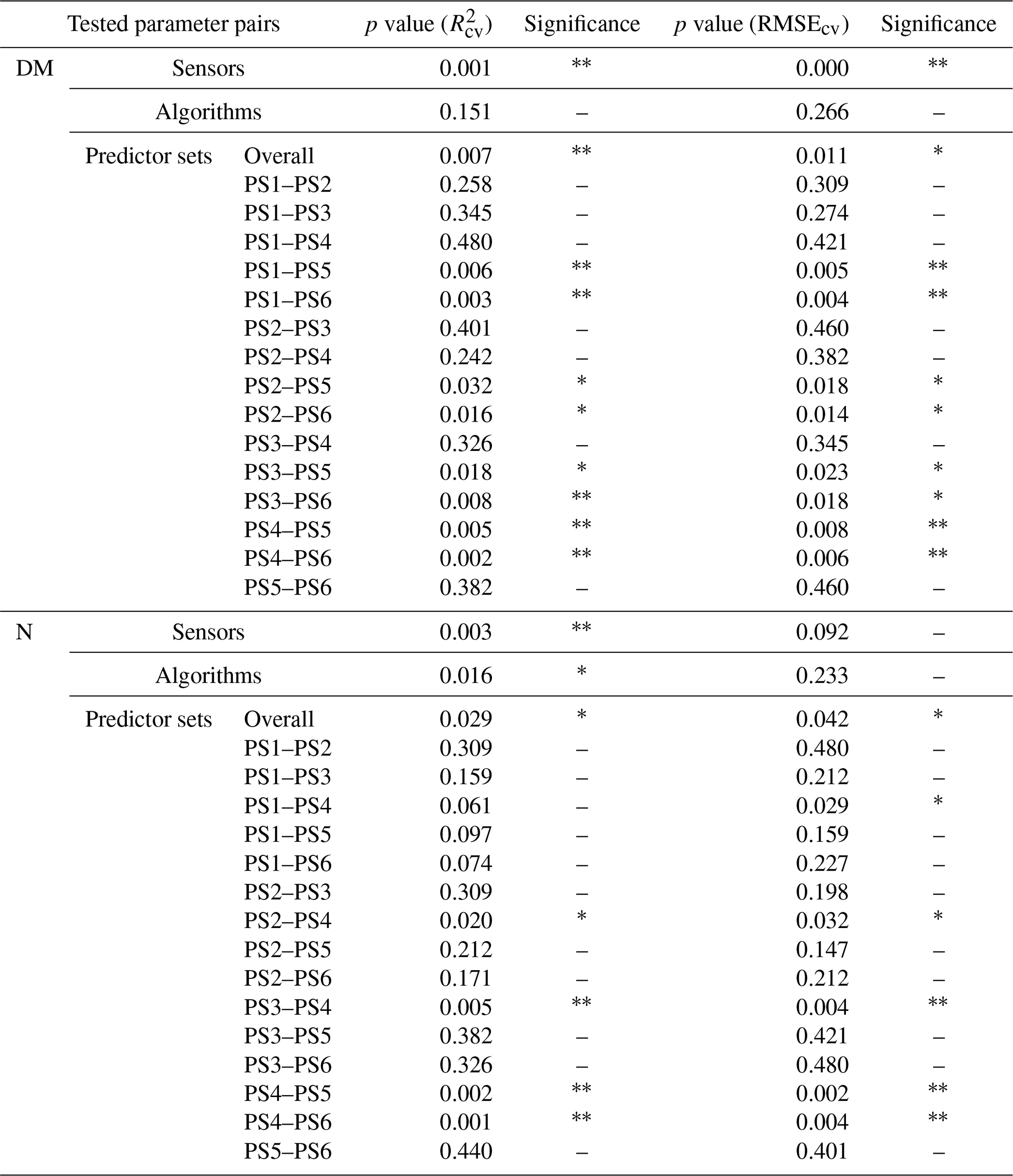
Symbols for significance level: p≤0.01, ∗ p≤0.05, – p>0.05.
The code used in the preparation of this paper is available upon request from the authors.
The field data set used in this study is available in the PANGAEA repository at https://doi.org/10.1594/PANGAEA.920600 (Schucknecht et al., 2020b).
The supplement related to this article is available online at: https://doi.org/10.5194/bg-19-2699-2022-supplement.
AS conceptualized the project and its methodology; performed data curation, data visualization, and the formal analysis; conducted the investigation; administered the project; and wrote the original draft of the paper. BS performed data curation and the formal analysis, conducted the investigation, designed the project's methodology, implemented software for the investigation, validated the results, visualized the data, and wrote the original draft of the paper. AK performed the formal analysis, acquired funding, conducted the investigation, provisioned resources, and reviewed and edited the paper. SA designed the project's methodology and wrote the original draft of the paper. CA reviewed and edited the paper. RK acquired funding, conducted the investigation, administered the project, and reviewed and edited the paper.
The contact author has declared that neither they nor their co-authors have any competing interests.
Publisher’s note: Copernicus Publications remains neutral with regard to jurisdictional claims in published maps and institutional affiliations.
We thank our colleagues from IMK-IFU, KIT, for their great support during the field and laboratory work and the IT department for supporting data processing and model running; our partners from the Technical University of Munich for the N analysis; Kerstin Grant from Agricultural Centre Baden-Württemberg (LAZBW) for the determination of the phenological stages of the plots; SAPOS for providing correction data; and the local farmers for their cooperation. We also gratefully acknowledge the computational and data resources provided by the Leibniz Supercomputing Centre (https://www.lrz.de, last access: 19 May 2022; project no. pn69tu). Furthermore, we thank Andreas Ibrom for handling the paper as an editor and Francesco Fava and one anonymous referee for their valuable comments.
This research has been supported by the German Federal Ministry of Education and Research (grant nos. 031B0027A, 031B0516A, 031B0027E, 031B0516E, and 031B0516F) via the SUSALPS project (https://www.susalps.de/, last access: 19 May 2022). BS has been supported by the Seventh framework programme of the European Community (grant no. 603416) and the Helmholtz Association.
The article processing charges for this open-access publication were covered by the Karlsruhe Institute of Technology (KIT).
This paper was edited by Andreas Ibrom and reviewed by Francesco Fava and one anonymous referee.
Aasen, H., Honkavaara, E., Lucieer, A., and Zarco-Tejada, P. J.: Quantitative remote sensing at ultra-high resolution with UAV spectroscopy: A review of sensor technology, measurement procedures, and data correction workflows, Remote Sens., 10, 1091, https://doi.org/10.3390/rs10071091, 2018.
Akaike, H.: Information theory and an extension of the maximum likelihood principle, in: Proceedings of the 2nd International Symposium on Information Theory, Budapest, 267–281, 1973.
Arlot, S. and Celisse, A.: A survey of cross-validation procedures for model selection, Statist. Surv., 4, 40–79, https://doi.org/10.1214/09-SS054, 2010.
Asam, S.: Potential of high resolution remote sensing data for Leaf Area Index derivation using statistical and physical models, PHD thesis, Julius-Maximilians-University Würzburg, Würzburg, 228 pp., 2014.
Assmann, J. J., Kerby, J. T., Cunliffe, A. M., and Myers-Smith, I. H.: Vegetation monitoring using multispectral sensors – best practices and lessons learned from high latitudes, J. Unmanned Veh. Sys., 7, 54–75, https://doi.org/10.1139/juvs-2018-0018, 2018.
Atzberger, C.: Advances in remote sensing of agriculture: Context description, existing operational monitoring systems and major information needs, Remote Sens., 5, 949–981, https://doi.org/10.3390/rs5020949, 2013.
Atzberger, C., Richter, K., Vuolo, F., Darvishzadeh, R., and Schlerf, M.: Why confining to vegetation indices?, Exploiting the potential of improved spectral observations using radiative transfer models, Remote Sensing for Agriculture, Ecosystems, and Hydrology XIII, 8174, 263–278, 2011.
Atzberger, C., Darvishzadeh, R., Immitzer, M., Schlerf, M., Skidmore, A., and le Maire, G.: Comparative analysis of different retrieval methods for mapping grassland leaf area index using airborne imaging spectroscopy, Int. J. Appl. Earth Obs., 43, 19–31, https://doi.org/10.1016/j.jag.2015.01.009, 2015.
Baret, F. and Buis, S.: Estimating canopy characteristics from remote sensing observations: review of methods and associated problems, in: Advances in Land Remote Sensing: System, Modeling, Inversion and Application, edited by: Liang, S., Springer Netherlands, Dordrecht, 173–201, 2008.
Baret, F. and Guyot, G.: Potentials and limits of vegetation indices for LAI and APAR assessment, Remote Sens. Environ., 35, 161–173, https://doi.org/10.1016/0034-4257(91)90009-U, 1991.
Bareth, G. and Schellberg, J.: Replacing manual rising plate meter measurements with low-cost UAV-derived sward height data in grasslands for spatial monitoring, PFG, 86, 157–168, https://doi.org/10.1007/s41064-018-0055-2, 2018.
Berger, K., Verrelst, J., Féret, J.-B., Hank, T., Wocher, M., Mauser, W., and Camps-Valls, G.: Retrieval of aboveground crop nitrogen content with a hybrid machine learning method, Int. J. Appl. Earth Obs., 92, 102174, https://doi.org/10.1016/j.jag.2020.102174, 2020.
Bernard, S., Heutte, L., and Adam, S.: Influence of hyperparameters on random forest accuracy, in: Multiple Classifier Systems, vol. 5519, edited by: Benediktsson, J. A., Kittler, J., and Roli, F., Springer Berlin Heidelberg, Berlin, Heidelberg, 171–180, https://doi.org/10.1007/978-3-642-02326-2_18, 2009.
Bischl, B., Wessing, S., Bauer, N., Friedrichs, K., and Weihs, C.: MOI-MBO: Multiobjective infill for parallel model-based optimization, in: Learning and Intelligent Optimization, Springer, Cham, 173–186, https://doi.org/10.1007/978-3-319-09584-4_17, 2014.
Breiman, L.: Random Forests, Mach. Learn., 45, 5–32, https://doi.org/10.1023/A:1010933404324, 2001.
Brooks, S. P. and Gelman, A.: General methods for monitoring convergence of iterative simulations, J. Comput. Graph. Stat., 7, 434–455, https://doi.org/10.2307/1390675, 1998.
Burai, P., Tomor, T., Bekő, L., and Deák, B.: Airborne hyperspectral remote sensing for identification grassland vegetation, Int. Arch. Photogramm. Remote Sens. Spatial Inf. Sci., XL-3/W3, 427–431, https://doi.org/10.5194/isprsarchives-XL-3-W3-427-2015, 2015.
Capolupo, A., Kooistra, L., Berendonk, C., Boccia, L., and Suomalainen, J.: Estimating plant traits of grasslands from UAV-acquired hyperspectral images: a comparison of statistical approaches, SPRS International Journal of Geo-Information, 4, 2792–2820, https://doi.org/10.3390/ijgi4042792, 2015.
Caruana, R. and Niculescu-Mizil, A.: An empirical comparison of supervised learning algorithms, in: Proceedings of the 23rd International Conference on Machine Learning, Pittsburgh, Pennsylvania, USA, Proceedings of the 23rd international conference on Machine learning, 161–168, https://doi.org/10.1145/1143844.1143865, 2006.
Caturegli, L., Corniglia, M., Gaetani, M., Grossi, N., Magni, S., Migliazzi, M., Angelini, L., Mazzoncini, M., Silvestri, N., Fontanelli, M., Raffaelli, M., Peruzzi, A., and Volterrani, M.: Unmanned aerial vehicle to estimate nitrogen status of turfgrasses, PloS One, 11, e0158268, https://doi.org/10.1371/journal.pone.0158268, 2016.
Culbert, P. D., Pidgeon, A. M., St.-Louis, V., Bash, D., and Radeloff, V. C.: The impact of phenological variation on texture measures of remotely sensed imagery, IEEE J. Sel. Top. Appl., 2, 299–309, https://doi.org/10.1109/JSTARS.2009.2021959, 2009.
Darvishzadeh, R., Atzberger, C., Skidmore, A., and Schlerf, M.: Mapping grassland leaf area index with airborne hyperspectral imagery: A comparison study of statistical approaches and inversion of radiative transfer models, ISPRS J. Photogramm., 66, 894–906, https://doi.org/10.1016/j.isprsjprs.2011.09.013, 2011.
Datt, B.: Visible/near infrared reflectance and chlorophyll concentration in Eucalyptus leaves, Int. J. Remote Sens., 20, 2741–2759, https://doi.org/10.1080/014311699211778, 1999.
Dinno, A.: dunn.test: Dunn's test of multiple comparisons using rank sums, https://CRAN.R-project.org/package=dunn.test (last access: 10 September 2021), 2017.
Dunn, O. J.: Multiple comparisons using rank sums, Technometrics, 6, 241–252, https://doi.org/10.1080/00401706.1964.10490181, 1964.
DWD Climate Data Center: Multi-annual grids of precipitation height over Germany 1981–2010, version v1.0, https://opendata.dwd.de/climate_environment/CDC/grids_germany/multi_annual/precipitation/, last access: 9 July 2019a.
DWD Climate Data Center: Multi-annual means of grids of air temperature (2 m) over Germany 1981–2010, version v1.0, https://opendata.dwd.de/climate_environment/CDC/grids_germany/multi_annual/air_temperature_mean/, last access: 9 July 2019b.
Egarter Vigl, L., Schirpke, U., Tasser, E., and Tappeiner, U.: Linking long-term landscape dynamics to the multiple interactions among ecosystem services in the European Alps, Landscape Ecol., 31, 1903–1918, https://doi.org/10.1007/s10980-016-0389-3, 2016.
Egarter Vigl, L., Candiago, S., Marsoner, T., Pecher, C., Tasser, E., Jäger, H., Meisch, C., Rüdisser, J., Schirpke, U., Tappeiner, U., and Labadini, A.: Ecosystem services in the Alps: a short report, Eurac Research, Institute for Alpine Environment, Bolzano/Bozen, 2018.
European Environmental Agency: Europe's ecological backbone: recognising the true value of our mountains, European Environmental Agency, Copenhagen, ISBN 978-92-9213-108-1 2010.
Ewald, J., Von Heßberg, A., Diewald, W., Rösler, S., Klotz, J., Fütterer, S., Eibes, P., and Jentsch, A.: Erfassung der Farn- und Blütenpflanzenarten auf der Wiederbeweidungsfläche am Brunnenkopf-Südhang (Ammergebirge), Berichte der Bayerischen Botanischen Gesellschaft, 88, 128–132, 2018.
Fernández-Delgado, M., Cernadas, E., Barro, S., and Amorim, D.: Do we need hundreds of classifiers to solve real world classification problems?, J. Mach. Learn. Res., 15, 3133–3181, 2014.
Fernández-Delgado, M., Sirsat, M., Cernadas, E., Alawadi, S., Barro, S., and Febrero-Bande, M.: An extensive experimental survey of regression methods, Neural Networks, 111, 11–34, https://doi.org/10.1016/j.neunet.2018.12.010, 2019.
Fontana, V., Radtke, A., Walde, J., Tasser, E., Wilhalm, T., Zerbe, S., and Tappeiner, U.: What plant traits tell us: Consequences of land-use change of a traditional agro-forest system on biodiversity and ecosystem service provision, Agr. Ecosyst. Environ., 186, 44–53, https://doi.org/10.1016/j.agee.2014.01.006, 2014.
Friedman, J. H.: Greedy function approximation: A gradient boosting machine, Ann. Statist., 29, 1189–1232, https://doi.org/10.1214/aos/1013203451, 2001.
Friedman, J. H.: Stochastic gradient boosting. Computational statistics & data analysis, 38, 367–378, https://doi.org/10.1016/S0167-9473(01)00065-2, 2002.
Gallardo-Cruz, J. A., Meave, J. A., González, E. J., Lebrija-Trejos, E. E., Romero-Romero, M. A., Pérez-García, E. A., Gallardo-Cruz, R., Hernández-Stefanoni, J. L., and Martorell, C.: Predicting Tropical Dry Forest Successional Attributes from Space: Is the Key Hidden in Image Texture?, PLOS ONE, 7, e30506, https://doi.org/10.1371/journal.pone.0030506, 2012.
Gelman, A. and Rubin, D. B.: A single series from the Gibbs sampler provides a false sense of security, Bayesian Statistics, 4, 625–631, 1992.
Gibson, D. J.: Grasses and grassland ecology, Oxford University Press, Oxford, 305 pp., 2009.
Greenwell, B., Boehmke, B., Cunningham, J., and GBM Developers: gbm: generalized boosted regression models, https://cran.r-project.org/web/packages/gbm/index.html (last access: 10 September 2021), 2020.
Grüner, E., Astor, T., and Wachendorf, M.: Biomass prediction of heterogeneous temperate grasslands using an SfM approach based on UAV imaging, Agronomy, 9, 54, https://doi.org/10.3390/agronomy9020054, 2019.
Grüner, E., Wachendorf, M., and Astor, T.: The potential of UAV-borne spectral and textural information for predicting aboveground biomass and N fixation in legume-grass mixtures, PLOS ONE, 15, e0234703, https://doi.org/10.1371/journal.pone.0234703, 2020.
Guan, S., Fukami, K., Matsunaka, H., Okami, M., Tanaka, R., Nakano, H., Sakai, T., Nakano, K., Ohdan, H., and Takahashi, K.: Assessing correlation of high-resolution NDVI with fertilizer application level and yield of rice and wheat crops using small UAVs, Remote Sens., 11, 112, https://doi.org/10.3390/rs11020112, 2019.
Handique, B. K., Khan, A. Q., Goswami, C., Prashnani, M., Gupta, C., and Raju, P. L. N.: Crop discrimination using multispectral sensor onboard unmanned aerial vehicle, P. Natl. Acad. Sci. USA, 87, 713–719, https://doi.org/10.1007/s40010-017-0443-9, 2017.
Hengl, T., Nussbaum, M., Wright, M. N., Heuvelink, G. B. M., and Gräler, B.: Random forest as a generic framework for predictive modeling of spatial and spatio-temporal variables, Peer J., 6, e5518, https://doi.org/10.7717/peerj.5518, 2018.
Jay, S., Gorretta, N., Morel, J., Maupas, F., Bendoula, R., Rabatel, G., Dutartre, D., Comar, A., and Baret, F.: Estimating leaf chlorophyll content in sugar beet canopies using millimeter- to centimeter-scale reflectance imagery, Remote Sens. Environ., 198, 173–186, https://doi.org/10.1016/j.rse.2017.06.008, 2017.
Jay, S., Baret, F., Dutartre, D., Malatesta, G., Héno, S., Comar, A., Weiss, M., and Maupas, F.: Exploiting the centimeter resolution of UAV multispectral imagery to improve remote-sensing estimates of canopy structure and biochemistry in sugar beet crops, Remote Sens. Environ., 231, 110898, https://doi.org/10.1016/j.rse.2018.09.011, 2019.
Jin, X., Liu, S., Baret, F., Hemerlé, M., and Comar, A.: Estimates of plant density of wheat crops at emergence from very low altitude UAV imagery, Remote Sens. Environ., 198, 105–114, https://doi.org/10.1016/j.rse.2017.06.007, 2017.
Kiese, R., Fersch, B., Baessler, C., Brosy, C., Butterbach-Bahl, K., Chwala, C., Dannenmann, M., Fu, J., Gasche, R., Grote, R., Jahn, C., Klatt, J., Kunstmann, H., Mauder, M., Rödiger, T., Smiatek, G., Soltani, M., Steinbrecher, R., Völksch, I., Werhahn, J., Wolf, B., Zeeman, M., and Schmid, H. P.: The TERENO pre-Alpine observatory: integrating meteorological, hydrological, and biogeochemical measurements and modeling, Vadose Zone J., 17, 180060, https://doi.org/10.2136/vzj2018.03.0060, 2018.
Kim, D.-G., Bond-Lamberty, B., Ryu, Y., Seo, B., and Papale, D.: Ideas and perspectives: Enhancing research and monitoring of carbon pools and land-to-atmosphere greenhouse gases exchange in developing countries, Biogeosciences, 19, 1435–1450, https://doi.org/10.5194/bg-19-1435-2022, 2022.
Koukal, T. and Atzberger, C.: Potential of multi-angular data derived from a digital aerial frame camera for forest classification, IEEE J. Sel. Top. Appl., 5, 30–43, https://doi.org/10.1109/JSTARS.2012.2184527, 2012.
Kruskal, W. H. and Wallis, W. A.: Use of ranks in one-criterion variance analysis, J. Am. Stat. Assoc., 47, 583–621, https://doi.org/10.1080/01621459.1952.10483441, 1952.
Kuhn, M. and Johnson, K.: Applied predictive modeling, Springer-Verlag, New York, ISBN 978-1-4614-6848-6, 2013.
Lamarque, P., Tappeiner, U., Turner, C., Steinbacher, M., Bardgett, R. D., Szukics, U., Schermer, M., and Lavorel, S.: Stakeholder perceptions of grassland ecosystem services in relation to knowledge on soil fertility and biodiversity, Reg. Environ. Change, 11, 791–804, https://doi.org/10.1007/s10113-011-0214-0, 2011.
Datasheet of Leica Viva GNSS GS10 receiver: https://w3.leica-geosystems.com/downloads123/zz/gpsgis/viva%20gnss/brochures-datasheet/leica_viva_gnss_gs10_receiver_ds_en.pdf last access: 7 June 2020.
Lumley, T.: leaps: regression subset selection (based on Fortran code by Alan Miller), https://CRAN.R-project.org/package=leaps (last access: 10 September 2021), 2020.
Lussem, U., Bolten, A., Menne, J., Gnyp, M. L., Schellberg, J., and Bareth, G.: Estimating biomass in temperate grassland with high resolution canopy surface models from UAV-based RGB images and vegetation indices, J. Appl. Remote Sens., 13, 1–26, 2019.
Lussem, U., Schellberg, J., and Bareth, G.: Monitoring forage mass with low-cost UAV data: Case study at the Rengen grassland experiment, PFG, 88, 407–422, https://doi.org/10.1007/s41064-020-00117-w, 2020.
Maes, W. H. and Steppe, K.: Perspectives for remote sensing with unmanned aerial vehicles in precision agriculture, Trends Plant Sci., 24, 152–164, https://doi.org/10.1016/j.tplants.2018.11.007, 2019.
Malkomes, G., Schaff, C., and Garnett, R.: Bayesian optimization for automated model selection, in: JMLR: Workshop and Conference Proceeding, ICML 2016 AutoML Workshop, New York, 41–47, 2016.
Marchese Robinson, R. L., Palczewska, A., Palczewski, J., and Kidley, N.: Comparison of the predictive performance and interpretability of random forest and linear models on benchmark data sets, J. Chem. Inf. Model., 57, 1773–1792, https://doi.org/10.1021/acs.jcim.6b00753, 2017.
Martinez-Cantin, R., de Freitas, N., Doucet, A., and Castellanos, J.: Active policy learning for robot planning and exploration under uncertainty, in: Robotics: Science and Systems III, Robotics: Science and Systems 2007, https://doi.org/10.15607/RSS.2007.III.041, 2007.
Maschler, J., Atzberger, C., and Immitzer, M.: Individual tree crown segmentation and classification of 13 tree species using airborne hyperspectral data, Remote Sens., 10, https://doi.org/10.3390/rs10081218, 2018.
Matsumura, K.: Unmanned Aerial Vehicle (UAV) for fertilizer management in grassland of Hokkaido, Japan, in: Unmanned Aerial Vehicle: Applications in Agriculture and Environment, edited by: Avtar, R. and Watanabe, T., Springer International Publishing, Cham, 39–50, https://doi.org/10.1007/978-3-030-27157-2_4, 2020.
Meier, U.: Growth stages of mono- and dicotyledonous plants: BBCH Monograph, Open Agrar Repositorium, Quedlinburg, https://doi.org/10.5073/20180906-074619, 2018
Meinshausen, N.: Quantile regression forests, J. Mach. Learn. Res., 7, 983–999, 2006.
Meinshausen, N.: quantregForest: quantile regression forests, https://CRAN.R-project.org/package=quantregForest (10 September 2021), 2017.
Moncayo-Cevallos, L. N., Rivadeneira-García, J. L., Andrade-Suárez, B. I., Leiva-González, C. A., González, I. S., Yépez-Campoverde, J. A., MaiguashcaGuzmán, J. A., and Toulkeridis, T.: A NDVI analysis contrasting different spectrum data methodologies applied in pasture crops previous grazing – a case study from Ecuador, in: 2018 International Conference on eDemocracy & eGovernment (ICEDEG), 2018 International Conference on eDemocracy & eGovernment (ICEDEG), 126–135, https://doi.org/10.1109/ICEDEG.2018.8372375, 2018.
Näsi, R., Viljanen, N., Kaivosoja, J., Alhonoja, K., Hakala, T., Markelin, L., and Honkavaara, E.: Estimating biomass and nitrogen amount of barley and grass using UAV and aircraft based spectral and photogrammetric 3D features, Remote Sens., 10, 1082, https://doi.org/10.3390/rs10071082, 2018.
Ollinger, S. V.: Sources of variability in canopy reflectance and the convergent properties of plants, New Phytol., 189, 375–394, https://doi.org/10.1111/j.1469-8137.2010.03536.x, 2011.
Olsson, P.-O., Vivekar, A., Adler, K., Garcia Millan, V. E., Koc, A., Alamrani, M., and Eklundh, L.: Radiometric correction of multispectral UAS images: Evaluating the accuracy of the Parrot Sequoia camera and sunshine sensor, Remote Sens., 13, 577, https://doi.org/10.3390/rs13040577, 2021.
Orzechowski, P., La Cava, W., and Moore, J. H.: Where are we now?, A large benchmark study of recent symbolic regression methods, in: Proceedings of the Genetic and Evolutionary Computation Conference, 1183–1190, 2018.
Poley, L. G. and McDermid, G. J.: A systematic review of the factors influencing the estimation of vegetation aboveground biomass using unmanned aerial systems, Remote Sens., 12, 1052 https://doi.org/10.3390/rs12071052, 2020.
Poncet, A. M., Knappenberger, T., Brodbeck, C., Fogle, M., Shaw, J. N., and Ortiz, B. V.: Multispectral UAS data accuracy for different radiometric calibration methods, Remote Sens., 11, 1917, https://doi.org/10.3390/rs11161917, 2019.
Primi, R., Filibeck, G., Amici, A., Bückle, C., Cancellieri, L., Di Filippo, A., Gentile, C., Guglielmino, A., Latini, R., Mancini, L. D., Mensing, S. A., Rossi, C. M., Rossini, F., Scoppola, A., Sulli, C., Venanzi, R., Ronchi, B., and Piovesan, G.: From Landsat to leafhoppers: A multidisciplinary approach for sustainable stocking assessment and ecological monitoring in mountain grasslands, Agr. Ecosyst. Environ., 234, 118–133, https://doi.org/10.1016/j.agee.2016.04.028, 2016.
Probst, P., Wright, M. N., and Boulesteix, A.-L.: Hyperparameters and tuning strategies for random forest, WIREs Data Mining and Knowledge Discovery, 9, e1301, https://doi.org/10.1002/widm.1301, 2019.
Pullanagari, R. R., Dynes, R. A., King, W. M., Yule, I. J., Thulin, S., Knox, N. M., and Ramoelo, A.: Remote sensing of pasture quality, in: Revitalising grasslands to sustain our communities, 22nd International Grassland Congress, Sydney, 633–638, 2013.
Pullanagari, R. R., Kereszturi, G., and Yule, I. J.: Mapping of macro and micro nutrients of mixed pastures using airborne AisaFENIX hyperspectral imagery, ISPRS J. Photogramm., 117, 1–01, https://doi.org/10.1016/j.isprsjprs.2016.03.010, 2016.
R Core Team: R: A language and environment for statistical computing, R Foundation for Statistical Computing, Vienna, Austria, https://www.R-project.org/, last access: 10 September 2021.
Richter, K., Hank, T. B., Mauser, W., and Atzberger, C.: Derivation of biophysical variables from Earth observation data: validation and statistical measures, J. Appl. Remote Sens., 6, 1–23, https://doi.org/10.1117/1.JRS.6.063557, 2012.
Richter, R.: Correction of satellite imagery over mountainous terrain, Appl. Opt., 37, 4004–4015, https://doi.org/10.1364/AO.37.004004, 1998.
Rossi, C., Kneubühler, M., Schütz, M., Schaepman, M. E., Haller, R. M., and Risch, A. C.: From local to regional: Functional diversity in differently managed alpine grasslands, Remote Sens. Environ., 236, 111415, https://doi.org/10.1016/j.rse.2019.111415, 2020.
Rossini, M., Cogliati, S., Meroni, M., Migliavacca, M., Galvagno, M., Busetto, L., Cremonese, E., Julitta, T., Siniscalco, C., Morra di Cella, U., and Colombo, R.: Remote sensing-based estimation of gross primary production in a subalpine grassland, Biogeosciences, 9, 2565–2584, 2012.
Rubel, F., Brugger, K., Haslinger, K., and Auer, I.: The climate of the European Alps: Shift of very high resolution Köppen-Geiger climate zones 1800–2100, Meteorol. Z., 26, 115–125, https://doi.org/10.1127/metz/2016/0816, 2017.
Salamí, E., Barrado, C., and Pastor, E.: UAV flight experiments applied to the remote sensing of vegetated areas, Remote Sens., 6, 11051–11081, https://doi.org/10.3390/rs61111051, 2014.
Schirpke, U., Kohler, M., Leitinger, G., Fontana, V., Tasser, E., and Tappeiner, U.: Future impacts of changing land-use and climate on ecosystem services of mountain grassland and their resilience, Ecosyst. Serv., 26, 79–94, https://doi.org/10.1016/j.ecoser.2017.06.008, 2017.
Schlingmann, M., Tobler, U., Berauer, B., Garcia-Franco, N., Wilfahrt, P., Wiesmeier, M., Jentsch, A., Wolf, B., Kiese, R., and Dannenmann, M.: Intensive slurry management and climate change promote nitrogen mining from organic matter-rich montane grassland soils, Plant Soil, 456, 81–98, https://doi.org/10.1007/s11104-020-04697-9, 2020.
Schuchardt, M. A. and Jentsch, A.: Plant species richness and cover in pre-Alpine grasslands of southern Germany, PANGAEA, https://doi.pangaea.de/10.1594/PANGAEA.920599, 2020.
Schucknecht, A., Krämer, A., Asam, S., Mejia Aguilar, A., Garcia Franco, N., Schuchardt, M. A., Jentsch, A., and Kiese, R.: Vegetation traits of pre-Alpine grasslands in southern Germany, Sci. Data, 7, 316, https://doi.org/10.1038/s41597-020-00651-7, 2020a.
Schucknecht, A., Krämer, A., Asam, S., Mejia Aguilar, A., Garcia Franco, N., Schuchardt, M. A., Jentsch, A., and Kiese, R.: In-situ reference data for aboveground vegetation traits of pre-Alpine grasslands in southern Germany, PANGAEA [data set], https://doi.org/10.1594/PANGAEA.920600, 2020b.
Seo, B., Bogner, C., Koellner, T., and Reineking, B.: Mapping fractional land use and land cover in a monsoon region: The effects of data processing options, IEEE J. Sel. Top. Appl., 9, 3941–3956, 2016.
Shahriari, B., Swersky, K., Wang, Z., Adams, R. P., and de Freitas, N.: Taking the human out of the loop: A review of Bayesian optimization, Proc. IEEE, 104, 148–175, https://doi.org/10.1109/JPROC.2015.2494218, 2016.
Song, Y. and Wang, J.: Winter wheat canopy height extraction from UAV-based point cloud data with a moving cuboid filter, Remote Sens., 11, https://doi.org/10.3390/rs11101239, 2019.
Spiegelberger, T., Matthies, D., Müller-Schärer, H., and Schaffner, U.: Scale-dependent effects of land use on plant species richness of mountain grassland in the European Alps, Ecography, 29, 541–548, 2006.
Strobl, C., Malley, J., and Tutz, G.: An introduction to recursive partitioning: Rationale, application, and characteristics of classification and regression trees, bagging, and random forests, Psychol. Methods, 14, 323–348, https://doi.org/10.1037/a0016973, 2009.
Stroppiana, D., Villa, P., Sona, G., Ronchetti, G., Candiani, G., Pepe, M., Busetto, L., Migliazzi, M., and Boschetti, M.: Early season weed mapping in rice crops using multi-spectral UAV data, Int. J. Remote Sens., 39, 5432–5452, https://doi.org/10.1080/01431161.2018.1441569, 2018.
Swersky, K., Snoek, J., and Adams, R. P.: Multi-task Bayesian optimization, in: Advances in Neural Information Processing Systems, 2004–2012, 2013.
Tsouros, D. C., Bibi, S. and Sarigiannidis, P. G.: A review on UAV-based applications for precision agriculture, Information, 10, 349, https://doi.org/10.3390/info10110349, 2019.
Vabalas, A., Gowen, E., Poliakoff, E., and Casson, A. J.: Machine learning algorithm validation with a limited sample size, PLOS ONE, 14, e0224365, https://doi.org/10.1371/journal.pone.0224365, 2019.
Väre, H., Lampinen, R., Humphries, C., and Williams, P.: Taxonomic diversity of vascular plants in the European alpine areas, in: Alpine Biodiversity in Europe, edited by: Nagy, L., Grabherr, G., Körner, C., and Thompson, D. B. A., Springer Berlin Heidelberg, Berlin, Heidelberg, 133–148, https://doi.org/10.1007/978-3-642-18967-8_5, 2003.
Varma, S. and Simon, R.: Bias in error estimation when using cross-validation for model selection, BMC Bioinf., 7, 91, https://doi.org/10.1186/1471-2105-7-91, 2006.
Veen, P., Jefferson, R., de, Smidt, J., and van der Straaten, J.: Grasslands in Europe, KNNV Publishing, Leiden, The Netherlands, ISBN 978-90-04-27810-3, 2009.
Verger, A., Vigneau, N., Chéron, C., Gilliot, J.-M., Comar, A., and Baret, F.: Green area index from an unmanned aerial system over wheat and rapeseed crops, Remote Sens. Environ., 152, 654–664, https://doi.org/10.1016/j.rse.2014.06.006, 2014.
Viljanen, N., Honkavaara, E., Näsi, R., Hakala, T., Niemeläinen, O., and Kaivosoja, J.: A novel machine learning method for estimating biomass of grass swards using a photogrammetric canopy height model, images and vegetation indices captured by a drone, Agriculture, 8, 70, https://doi.org/10.3390/agriculture8050070, 2018.
Wachendorf, M., Fricke, T., and Möckel, T.: Remote sensing as a tool to assess botanical composition, structure, quantity and quality of temperate grasslands, Grass Forage Sci., 73, 1–14, https://doi.org/10.1111/gfs.12312, 2017.
Walter, J., Grant, K., Beierkuhnlein, C., Kreyling, J., Weber, M., and Jentsch, A.: Increased rainfall variability reduces biomass and forage quality of temperate grassland largely independent of mowing frequency, Agr. Ecosyst. Environ., 148, 1–10, https://doi.org/10.1016/j.agee.2011.11.015, 2012.
Wang, D., Xin, X., Shao, Q., Brolly, M., Zhu, Z., and Chen, J.: Modeling aboveground biomass in Hulunber grassland ecosystem by using unmanned aerial vehicle discrete lidar, Sensors, 17, 180, https://doi.org/10.3390/s17010180, 2017.
White, R. P., Murray, S., and Rohweder, M.: Pilot analysis of globale ecosystems – Grassland ecosystems, World Resources Institute, ISBN 1-56973-461-5, 2000.
Wiesmeier, M., Hübner, R., Barthold, F., Spörlein, P., Geuß, U., Hangen, E., Reischl, A., Schilling, B., von Lützow, M., and Kögel-Knabner, I.: Amount, distribution and driving factors of soil organic carbon and nitrogen in cropland and grassland soils of southeast Germany (Bavaria), Agr. Ecosyst. Environ., 176, 39–52, https://doi.org/10.1016/j.agee.2013.05.012, 2013.
Wijesingha, J., Moeckel, T., Hensgen, F., and Wachendorf, M.: Evaluation of 3D point cloud-based models for the prediction of grassland biomass, Int. J. Appl. Earth Obs. Geoinf., 78, 352–359, https://doi.org/10.1016/j.jag.2018.10.006, 2019.
Wijesingha, J., Astor, T., Schulze-Brüninghoff, D., Wengert, M., and Wachendorf, M.: Predicting forage quality of grasslands using UAV-borne imaging spectroscopy, Remote Sens., 12, https://doi.org/10.3390/rs12010126, 2020.
Wilcoxon, F.: Individual comparisons by ranking methods, Biometrics Bull., 1, 80–83, https://doi.org/10.2307/3001968, 1945.
Yao, X., Wang, N., Liu, Y., Cheng, T., Tian, Y., Chen, Q., and Zhu, Y.: Estimation of wheat LAI at middle to high levels using unmanned aerial vehicle narrowband multispectral imagery, Remote Sens., 9, 1304, https://doi.org/10.3390/rs9121304, 2017.
Zacharias, S., Bogena, H., Samaniego, L., Mauder, M., Fuß, R., Pütz, T., Frenzel, M., Schwank, M., Baessler, C., Butterbach-Bahl, K., Bens, O., Borg, E., Brauer, A., Dietrich, P., Hajnsek, I., Helle, G., Kiese, R., Kunstmann, H., Klotz, S., Munch, J. C., Papen, H., Priesack, E., Schmid, H. P., Steinbrecher, R., Rosenbaum, U., Teutsch, G., and Vereecken, H.: A network of terrestrial environmental observatories in Germany, Vadose Zone J., 10, 955–973, https://doi.org/10.2136/vzj2010.0139, 2011.
Zhang, H., Sun, Y., Chang, L., Qin, Y., Chen, J., Qin, Y., Du, J., Yi, S., and Wang, Y.: Estimation of grassland canopy height and aboveground biomass at the quadrat scale using unmanned aerial vehicle, Remote Sens., 10, 851, https://doi.org/10.3390/rs10060851, 2018.
Ziliani, G. M., Parkes, D. S., Hoteit, I., and McCabe, F. M.: Intra-season crop height variability at commercial farm scales using a fixed-wing UAV, Remote Sens., 10, 2007, https://doi.org/10.3390/rs10122007, 2018.
Zistl-Schlingmann, M., Kwatcho Kengdo, S., Kiese, R., and Dannenmann, M.: Management intensity controls nitrogen-use-efficiency and flows in grasslands – A 15∘ N tracing experiment, Agronomy, 10, 606, https://doi.org/10.3390/agronomy10040606, 2020.