the Creative Commons Attribution 4.0 License.
the Creative Commons Attribution 4.0 License.
 | 19 Jan 2022
Temporal dynamics of surface ocean carbonate chemistry in response to natural and simulated upwelling events during the 2017 coastal El Niño near Callao, Peru
Ulf Riebesell
Kai G. Schulz
Elisabeth von der Esch
Eric P. Achterberg
Lennart T. Bach
Oxygen minimum zones (OMZs) are characterized by enhanced carbon dioxide (CO2) levels and low pH and are being further acidified by uptake of anthropogenic atmospheric CO2. With ongoing intensification and expansion of OMZs due to global warming, carbonate chemistry conditions may become more variable and extreme, particularly in the eastern boundary upwelling systems. In austral summer (February–April) 2017, a large-scale mesocosm experiment was conducted in the coastal upwelling area off Callao (Peru) to investigate the impacts of ongoing ocean deoxygenation on biogeochemical processes, coinciding with a rare coastal El Niño event. Here we report on the temporal dynamics of carbonate chemistry in the mesocosms and surrounding Pacific waters over a continuous period of 50 d with high-temporal-resolution observations (every second day). The mesocosm experiment simulated an upwelling event in the mesocosms by addition of nitrogen (N)-deficient and CO2-enriched OMZ water. Surface water in the mesocosms was acidified by the OMZ water addition, with pHT lowered by 0.1–0.2 and pCO2 elevated to above 900 µatm. Thereafter, surface pCO2 quickly dropped to near or below the atmospheric level (405.22 µatm in 2017; Dlugokencky and Tans, 2021; NOAA/Global Monitoring Laboratory (GML)) mainly due to enhanced phytoplankton production with rapid CO2 consumption. Further observations revealed that the dominance of the dinoflagellate Akashiwo sanguinea and contamination of bird excrements played important roles in the dynamics of carbonate chemistry in the mesocosms. Compared to the simulated upwelling, natural upwelling events in the surrounding Pacific waters occurred more frequently with sea-to-air CO2 fluxes of 4.2–14.0 mmol C m−2 d−1. The positive CO2 fluxes indicated our site was a local CO2 source during our study, which may have been impacted by the coastal El Niño. However, our observations of dissolved inorganic carbon (DIC) drawdown in the mesocosms suggest that CO2 fluxes to the atmosphere can be largely dampened by biological processes. Overall, our study characterized carbonate chemistry in nearshore Pacific waters that are rarely sampled in such a temporal resolution and hence provided unique insights into the CO2 dynamics during a rare coastal El Niño event.
- Article
(4280 KB) - Full-text XML
-
Supplement
(789 KB) - BibTeX
- EndNote


One of the most extensive oxygen minimum zones (OMZs) in the global ocean can be found off central/northern Peru (4–16∘ S; Chavez and Messié, 2009). High biological productivity is stimulated by permanent upwelling of cold, nutrient-rich water to the surface, supporting remarkable fish production off Peru (Chavez et al., 2008; Montecino and Lange, 2009; Albert et al., 2010). The high primary production also leads to enhanced remineralization of sinking organic matter in subsurface waters which depletes dissolved oxygen (O2) and creates an intense and shallow OMZ (Chavez et al., 2008). The depletion of O2 in OMZs plays an important role in the global nitrogen (N) cycle, accounting for 20 %–40 % of N loss in the ocean (Lam et al., 2009; Paulmier and Ruiz-Pino, 2009). Denitrification and anammox processes that occur in O2-depleted waters remove biologically available N from the ocean and produce an N deficit and hence phosphorus (P) excess with respect to the Redfield ratio ( = ) in the water column (Redfield, 1963; Deutsch et al., 2001, 2007; Hamersley et al., 2007; Galán et al., 2009; Lam et al., 2009). Upwelling of this N-deficient water has been found to control the surface water nutrient stoichiometry and thus influence phytoplankton growth and community compositions (Franz et al., 2012; Hauss et al., 2012).
Apart from being N-deficient, the OMZ waters are also characterized by enhanced carbon dioxide (CO2) concentrations and low pH from respiratory processes and are further acidified by increasing anthropogenic atmospheric CO2 (Feely et al., 2008; Friederich et al., 2008; Paulmier et al., 2008, 2011). Accordingly, surface water carbonate chemistry is influenced by upwelling of CO2-enriched OMZ water (Van Geen et al., 2000; Capone and Hutchins, 2013). The upwelled CO2-enriched OMZ water can give rise to surface CO2 levels > 1000 µatm, pH values as low as 7.6, and under-saturation for the calcium carbonate mineral aragonite (Feely et al., 2008; Hauri et al., 2009). As a result, there is a significant flux of CO2 from the ocean to the atmosphere off Peru, which is further facilitated by surface ocean warming, making the Peruvian upwelling region a year-round CO2 source to the atmosphere (Friederich et al., 2008). In contrast, rapid utilization of upwelled CO2 and nutrients by phytoplankton can occasionally deplete surface CO2 below atmospheric equilibrium and dampen the CO2 outgassing (Van Geen et al., 2000; Friederich et al., 2008; Loucaides et al., 2012). The enhanced primary production in turn contributes to increasing export of organic matter, enhanced bacterial respiration, O2 consumption, and CO2 production at depth. Such a positive feedback may determine the intensity of the underlying OMZ and promote carbon (C) preservation in marine sediments (Dale et al., 2015).
In response to reduced O2 solubility and enhanced stratification induced by global warming, OMZs have been intensifying and expanding over the past decades (Stramma et al., 2008, 2010; Fuenzalida et al., 2009). Based on regional observations and model projections, a decline in dissolved O2 concentrations has been reported for most regions of the global ocean (Matear et al., 2000; Matear and Hirst, 2003; Whitney et al., 2007; Stramma et al., 2008; Keeling et al., 2009; Bopp et al., 2013; Schmidtko et al., 2017; Oschlies et al., 2018). The vertical expansion of OMZs represents shoaling of CO2-enriched seawater, which has become further enriched by oceanic uptake of anthropogenic CO2 (Doney et al., 2012; Gilly et al., 2013; Schulz et al., 2019). Since biogeochemical processes in OMZs are directly linked to the C cycle and control surface nutrient stoichiometry, with ongoing ocean warming and acidification, the deoxygenation may have cascading effects on plankton productivity and composition, C uptake, and food web functioning (Keeling et al., 2009; Gruber, 2011; Doney et al., 2012; Gilly et al., 2013; Levin and Breitburg, 2015). Therefore, it is important to monitor the changes in CO2 when investigating the effects of deoxygenation on marine ecosystems.
To investigate the potential impacts of upwelling on pelagic biogeochemistry and natural plankton communities in the Peruvian OMZ, a large-scale in situ mesocosm study was carried out in the coastal upwelling area off Peru. An upwelling event was simulated in the mesocosms by addition of OMZ waters collected from two different locations where the OMZ was considered to contain different nutrient concentrations and N:P ratios. The ecological and biogeochemical responses in the mesocosms were monitored and compared with those influenced by natural upwelling events in the ambient coastal water surrounding the mesocosms. As part of this collaborative research project, questions specific to the present paper were as follows: (1) how does surface water carbonate chemistry respond to an upwelling event? And (2) how does upwelled OMZ water with different chemical signatures modulate surface water carbonate chemistry? The current study will mainly focus on the temporal changes in surface water carbonate chemistry within the individual mesocosms, including observations made in the ambient Pacific water and a local estimate of air–sea CO2 exchange, together with the influence of a rare coastal El Niño event (Garreaud, 2018). This provides first insights into how inorganic C cycling links to chemical signatures of OMZ waters in a natural plankton community and its implications for ongoing environmental changes.
2.1 Study site
The experiment was conducted in the framework of the Collaborative Research Center 754 “Climate-Biogeochemistry Interactions in the Tropical Ocean” (https://www.sfb754.de/en, last access: 16 June 2020) and in collaboration with the Instituto del Mar del Perú (IMARPE) in Callao, Peru (Fig. 1a). The coastal area off Callao lies within the Humboldt Current System and is influenced by wind-induced coastal upwelling (Bakun and Weeks, 2008).
2.2 Mesocosm setup
Eight Kiel Off-Shore Mesocosms for Future Ocean Simulations (KOSMOS) units (M1–M8), extending 19 m below the sea surface, were deployed by the research vessel Buque Armada Peruana (BAP) Morales and moored at 12.06∘ S, 77.23∘ W in the coastal upwelling area off Callao, Peru (Fig. 1a) on 23 February 2017 (late austral summer). The technical design of these seagoing mesocosms is described by Riebesell et al. (2013). For a more detailed description of the mesocosm deployment and maintenance in this study, please refer to Bach et al. (2020a).
The mesocosm bags were filled with surrounding seawater through the upper and lower openings. Both openings were covered by screens with a mesh size of 3 mm to avoid enclosing larger organisms such as fish. The mesocosm bags were left open below the water surface for 2 d, allowing free exchange with surrounding coastal water. On 25 February, mesocosm bags were closed with the screens removed, tops pulled above the sea surface, and bottoms sealed with 2 m long conical sediment traps (Fig. 1b). The experiment started with the closure of the mesocosms (day 0) and lasted for 50 d. Each mesocosm bag enclosed a seawater volume of ∼ 54 m3. After the bags were closed, daily or every-second-day sampling was performed to monitor the initial conditions of the enclosed water before simulating an upwelling event on day 11 and 12 (see Sect. 2.4 for details).
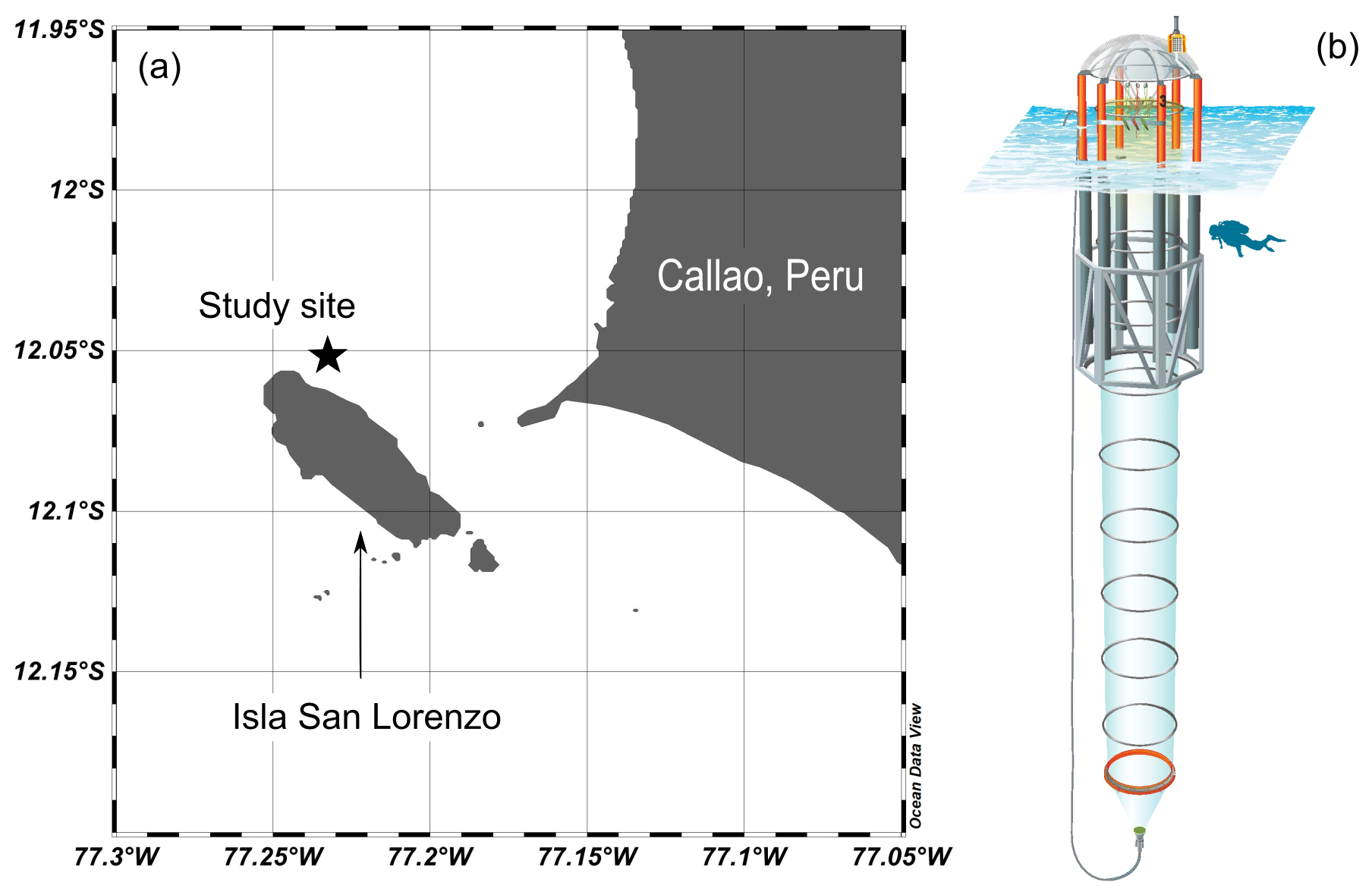
Figure 1The study site of the mesocosm experiment (a) created and modified using Ocean Data View (Reiner Schlitzer, Ocean Data View, https://odv.awi.de/, last access: 6 April 2021) and a schematic illustration of a KOSMOS mesocosm unit (b). We acknowledge reprint permission from the American Geophysical Union as parts of this drawing were used for a publication by Bach et al. (2016). The star symbol marks the approximate location of mesocosm deployment.
2.3 Simulated upwelling and salt addition
To simulate an upwelling event in the mesocosms, OMZ-influenced waters were collected from the nearby coastal area and added to the mesocosms. Two OMZ water masses were collected at Station 1 (12∘01.70′ S, 77∘13.41′ W) at a depth of ∼ 30 m and at Station 3 (12∘ 02.41′ S, 77∘22.50′ W) at a depth of ∼ 70 m, respectively, using a deep-water collection system as described by Taucher et al. (2017). These two water masses were sampled for chemical and biological variables as done in the mesocosms (see Sect. 2.4). The OMZ water collected from Station 3 had a dissolved inorganic nitrogen (DIN) concentration of 4.3 µmol L−1 (denoted as “Low DIN” in this paper) and was added to M2, M3, M6, and M7. The OMZ water from Station 1 had a DIN of 0.3 µmol L−1 (denoted as “Very low DIN” in this paper) and was added to M1, M4, M5, and M8. Before OMZ water addition, approximately 9 m3 of seawater was removed from 11–12 m of each mesocosm on 5 March (day 8). During the night of 8 March (day 11), ∼ 10 m3 of OMZ water was added to 14–17 m of each mesocosm. On 9 March (day 12), ∼ 10 m3 of seawater was removed from 8–9 m followed by an addition of ∼ 12 m3 OMZ water to 0–9 m of each mesocosm.
To maintain a low-O2 bottom layer in the mesocosms and avoid convective mixing induced by heat exchange with the surrounding Pacific, 69 L of a concentrated sodium chloride (NaCl) brine solution was added to the bottom of each mesocosm (10–17 m) on day 13, which increased the bottom salinity by ∼ 0.7 units. Following that, turbulent mixing induced by sampling activities continuously interrupted the artificial halocline. Hence, on day 33, 46 L of the NaCl brine solution was added again to the bottom of each mesocosm (12.5–17 m), which increased the bottom salinity by ∼ 0.5 units. At the end of the experiment after the last sampling (day 50), 52 kg of NaCl brine was added again to each mesocosm to calculate the enclosed seawater volume from a measured salinity change by ∼ 0.2 units (see Czerny et al., 2013a, and Schulz et al., 2013, for details). The average final volume for each mesocosm bag was calculated at ∼ 54 m3. With known sampling volumes and deep-water addition volumes during the experiment, the enclosed volumes of each mesocosm on each sampling day could be calculated. The NaCl solution for the halocline establishments had been prepared in Germany by dissolving 300 kg of food industry grade NaCl (free of anti-caking agents) in 1000 L of deionized water (Milli-Q, Millipore) and purified with ion exchange resin (Lewatit® MonoPlus TP 260, Lanxess, Germany) to minimize potential contaminations with trace metals (Czerny et al., 2013a). The NaCl solution for the volume determination was produced on-site using locally purchased table salt. For a more detailed description of OMZ water and salt additions, please refer to Bach et al. (2020a).
2.4 Sampling procedures and CTD operations
Sampling was carried out in the morning (07:00–11:00 local time) daily or every second day throughout the entire experimental period. Depth-integrated samples were taken from the surface (0–10 m for day 3–28) and bottom layer (10–17 m for day 3–28) of the mesocosms and the surrounding coastal water (named “Pacific”) using a 5 L integrating water sampler (IWS, HYDRO-BIOS, Kiel). Due to the deepening of the oxycline as observed from the CTD profiles, the sampling depth for the surface was adjusted to 0–12.5 m while that for the bottom was changed to 12.5–17 m from day 29 until the end of the experiment (day 50).
For gas-sensitive variables such as pH and dissolved inorganic carbon (DIC), 1.5 L of seawater from each integrated depth in each mesocosm was taken directly from the fully filled 5 L integrating water sampler. Clean polypropylene sampling bottles (rinsed with deionized water in the laboratory; Milli-Q, Millipore) were pre-rinsed with sample water immediately prior to sampling. Bottles were filled from bottom to top using pre-rinsed Tygon tubing with overflow of at least one sampling bottle volume (1.5 L) to minimize the impact of CO2 air–water gas exchange. Nutrient samples were collected into 250 mL polypropylene bottles using pre-rinsed Tygon tubing (see Bach et al., 2020a, for details). Sample containers were stored in cool boxes for ∼ 3 h and protected from sunlight and heat before being transported to the shore. Once in the lab, sample water was sterile-filtered by gentle pressure using syringe filters (0.2 µm pore size), Tygon tubing, and a peristaltic pump to remove particles that may cause changes to seawater carbonate chemistry (Bockmon and Dickson, 2014). For DIC measurements, the water was filtered from the bottom of the 1.5 L sample bottle into 100 mL glass-stoppered bottles (DURAN) with an overflow of at least 100 mL to minimize contact with air. Once the glass bottle was filled with sufficient overflow, it was immediately sealed without headspace using a round glass stopper. This procedure was repeated to collect a second bottle (100 mL) of filtered water for pH measurements. The leftover seawater was directly filtered into a 500 mL polypropylene bottle for total alkalinity (TA) measurements (non-gas-sensitive). Filtered DIC and pH samples were stored at 4 ∘C in the dark, and TA samples were at room temperature in the dark until further analysis. Samples were analyzed for DIC and pH on the same day of sampling, while TA was determined overnight (see Sect. 2.5 for analytical procedures).
CTD casts were performed with a multiparameter logging probe (CTD60M, Sea & Sun Technology) in the mesocosms and Pacific on every sampling day. From the CTD casts, profiles of salinity, temperature, pH, dissolved O2, chlorophyll a (chl a), and photosynthetically active radiation were obtained (see Schulz and Riebesell, 2013, and Bach et al., 2020a, for details).
2.5 Carbonate chemistry and nutrient measurements
Total alkalinity was determined at room temperature (22–32 ∘C) by a two-stage open-cell potentiometric titration using a Metrohm 862 Compact Titrosampler, Aquatrode Plus (Pt1000), and 907 Titrando unit in the IMARPE laboratory following Dickson et al. (2003). The acid titrant was prepared by preparing a 0.05 mol kg−1 hydrochloric acid (HCl) solution with an ionic strength of ca. 0.7 mol kg−1 (adjusted by NaCl). Approximately 50 g of sample water from each sample was weighed into the titration cell with the exact weight recorded (precision 0.0001 g). After the two-stage titration, the titration data between a pH of ∼ 3.5 and 3 were fitted to a modified non-linear Gran approach described in Dickson et al. (2007) using MATLAB (The MathWorks). The results were calibrated against certified reference material (CRM) batch 142 (Dickson, 2010) measured on each measurement day. In this paper, measured TA values refer to the measured values that have been calibrated against the CRM.
Seawater pHT (total scale) was determined spectrophotometrically by measuring the absorbance ratios after adding the indicator dye m-cresol purple (mCP) as described in Carter et al. (2013). Before measurements, samples were acclimated to 25.0 ∘C in a thermostatted bath. The absorbance of samples with mCP was determined on a Varian Cary 100 double-beam spectrophotometer (Varian), scanning between 780 and 380 nm at a 1 nm resolution. During the spectrophotometric measurement, the temperature of the sample was maintained at 25.0 ∘C by a water bath connected to the thermostatted 10 cm cuvette. The pHT values were calculated from the baseline-corrected absorbance ratios and corrected for in situ salinity (obtained from CTD casts) and pH change caused by dye addition (using the absorbance at the isosbestic point, i.e., 479 nm) as described in Dickson et al. (2007). To minimize potential CO2 air–water gas exchange, a syringe pump (Tecan Cavro XLP) was used for sample and dye mixing and cuvette injection (see Schulz et al., 2017, for details). For the dye correction, a batch of sterile filtered seawater of known salinity was prepared. The pHT was determined once for an addition of 7 µL of dye and once for an addition of 25 µL at five pH levels (raised to 7.95 with NaOH and lowered to 7.74, 7.58, 7.49, and 7.36 with HCl stepwise). The pH change resulting from the dye correction addition was calculated from the change in measured absorbance ratio for each pair of dye additions (see Clayton and Byrne, 1993, and Dickson et al., 2007, for details). The dye-corrected pHT values measured at 25.0 ∘C and atmospheric pressure were then re-calculated for in situ temperature and pressure as determined by CTD casts (averaged over 0–10/12.5 m for surface and 10/12.5–17 m for bottom). For carbonate chemistry speciation calculations (see Sect. 2.6), the dye-corrected pHT values were used as one of the input parameters.
Dissolved inorganic carbon was measured by infrared absorption using a LI-COR LI-7000 on an AIRICA system (MARIANDA, Kiel; see Taucher et al., 2017, and Gafar and Schulz, 2018, for details). The results were calibrated against CRM batch 142 (Dickson, 2010). Unfortunately, due to a malfunctioning of the AIRICA system, we obtained measured DIC data only up to 7 March (day 10). Therefore, measured TA and pHT were used for calculations of carbonate system parameters at in situ temperature and salinity, but we used DIC measurements from day 3–10 for consistency checks of calculated carbonate chemistry parameters. In this paper, measured DIC values refer to the measured values that have been calibrated against the CRM.
Inorganic nutrients were analyzed colorimetrically (NO, NO, PO, and Si(OH)4) and fluorimetrically (NH using a continuous-flow analyzer (QuAAtro AutoAnalyzer with integrated photometers, SEAL Analytical) connected to a fluorescence detector (FP-2020, JASCO). All colorimetric methods were conducted according to Murphy and Riley (1962), Mullin and Riley (1955a, b), and Morris and Riley (1963) and corrected following the refractive index method developed by Coverly et al. (2012). For details of the quality control procedures, see Bach et al. (2020a).
2.6 Carbonate chemistry speciation calculations and propagated uncertainties
Calculations of carbonate chemistry parameters (in situ pHT, DIC, pCO2, and calcium carbonate saturation state for calcite and aragonite) were performed with the Excel version of CO2SYS (Version 2.1; Pierrot et al., 2006) using K1 and K2 dissociation constants from Mehrbach et al. (1973) which were refitted by Lueker et al. (2000). The dissociation constants for KHSO4 from Dickson (1990) and for total boron from Uppström (1974) were applied in the calculations (see Orr et al., 2015, for details). The observed pHT and TA as well as inorganic nutrient concentration (phosphate and silicic acid) were used as input CO2 system parameters. In situ salinity and temperature were obtained by CTD casts and averaged over surface (0–10 or 0–12.5 m) and bottom (10–17 or 12.5–17 m) waters for each sampling day. In situ pressure was approximated for surface (5 dbar) and bottom (13.5 or 14.75 dbar) waters. For details of calculation procedures and choices of constants, see Lewis et al. (1998) and Orr et al. (2015).
To evaluate the performance of pHT and TA measurements, quality control procedures were performed. First, standard deviations of pHT measurements were graphed over time. Measured TA values of a control sample (CRM batch 142; Dickson, 2010) were plotted over time and compared to the warning and control limits calculated from their mean and standard deviation (for details please see Dickson et al., 2007) as well as the certified value of the CRM. To compute a range control chart for the evaluation of measurement repeatability, the absolute difference between duplicate measurements of CRMs on each sampling day was calculated and plotted over time and compared to the warning and control limits calculated from their mean and standard deviation (for details see Dickson et al., 2007).
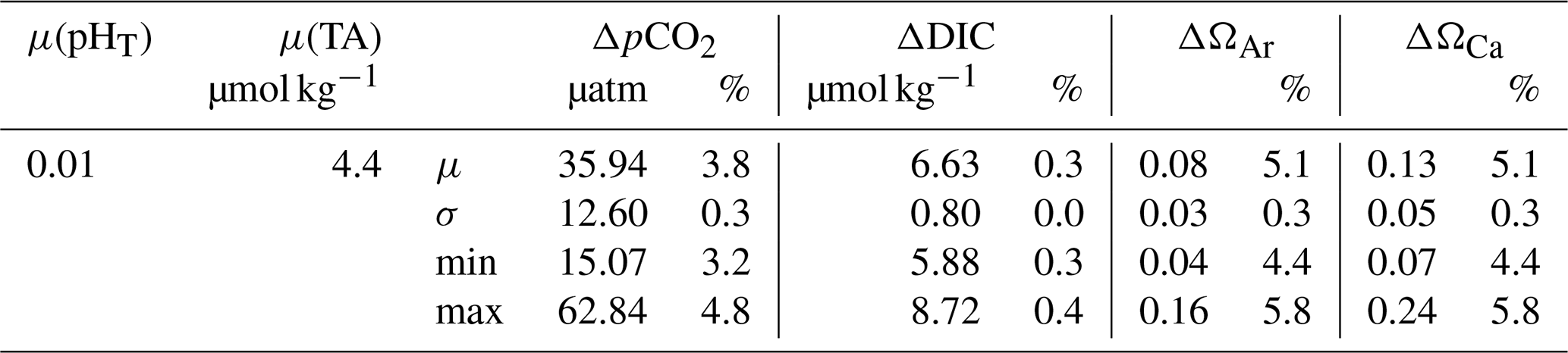
We used the R package “seacarb” with a Gaussian approach and an input variable pair (pHT, TA) to calculate uncertainties for calculated CO2 system parameters (Orr et al., 2018; Gattuso et al., 2020). The contributions of input uncertainties in nutrient concentrations and in situ salinity and temperature to the uncertainties in the CO2SYS-based calculations are often small (< 0.1 %; Orr et al., 2018), so they were not considered in our propagation. The input uncertainties in pHT and TA were estimated based on our measurements (Table 1). Standard uncertainties include random and systematic errors. For TA, systematic errors were removed by calibrating the measured results using CRMs (see Sect. 2.5). Hence, the random error in TA, estimated by the averaged standard deviation of all the CRM measurements (4.4 µmol kg−1; n=62), was used as the standard uncertainty. For pHT, an uncertainty of 0.01 was used as the standard uncertainty. Due to the unavailability of CRMs that correct for systematic error in pH measurements, the standard deviations of repeated measurements (0.0012; n=377) only accounted for the random components of standard uncertainties (Orr et al., 2018). Therefore, we used 0.01 in our uncertainty propagation as an approximation of the total standard uncertainty for pHT, which has been used in previous assessments (Orr et al., 2018).
Table 1Standard uncertainties in pHT and TA estimated based on our measurements are denoted by μ(pHT) and µ(TA). Based on μ(pHT) and μ(TA), propagated uncertainties were estimated for each data point in R and averaged for each reported variable (μ), with standard deviation (σ), minimum (min), and maximum (max) values presented. The relative percentages (%) of propagated standard uncertainties were calculated by dividing the propagated uncertainty by the corresponding data point and averaged for each reported variable (μ), with σ, min, and max values presented.
The air–sea flux of CO2 (FCO2, mmol C m−2 d−1) in the Pacific was determined based on
where k is the gas transfer velocity parameterized as a function of wind speed, K0 is the solubility of CO2 in seawater dependent on in situ salinity and temperature (Weiss, 1974), and ΔpCO2 is the difference between pCO2 in the surface water and in the atmosphere (Wanninkhof 2014). Wind data were averaged over 2 sampling days for the sampling location from a satellite-derived gridded dataset (Global Land Data Assimilation System model, near-surface wind speed, , 3 h temporal resolution, 12.375 to 11.875∘ S, 77.375 to 76.875∘ W), obtained from NASA Giovanni (Rodell et al., 2004; Beaudoing and Rodell, 2020). In situ salinity and temperature were obtained from the CTD casts (see Sect. 2.4). Calculated pCO2 based on (pHT, TA) and an estimated atmospheric pCO2 of 405.22 µatm (referenced to year 2017; Dlugokencky and Tans, 2021; NOAA/GML) were used in the air–sea flux estimation.
3.1 Responses of surface layer nutrient concentrations
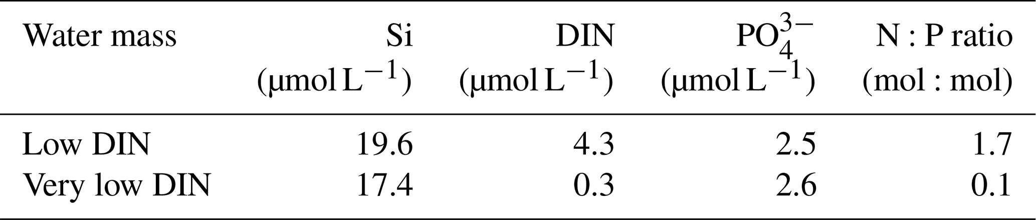
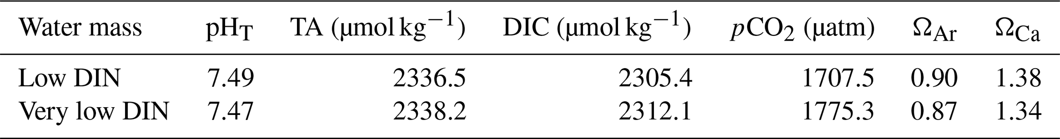
The OMZ-influenced water masses were collected from two locations and added to the mesocosms to simulate an upwelling event (see Sect. 2.3). The two water masses were named Low DIN and Very low DIN, respectively, based on their DIN concentrations (Table 2). Both water masses shared similar silicic acid (Si) and phosphate (PO concentrations but differed in DIN concentration. The Low DIN water had a DIN concentration of 4.3 µmol L−1, 14 times as high as that of the Very low DIN water (0.3 µmol L−1, Table 2).
Table 2Inorganic nutrient concentrations of the two collected deep-water masses. Please note that DIN is the sum of nitrate, nitrite, and ammonium. P is phosphate. Si is silicic acid.
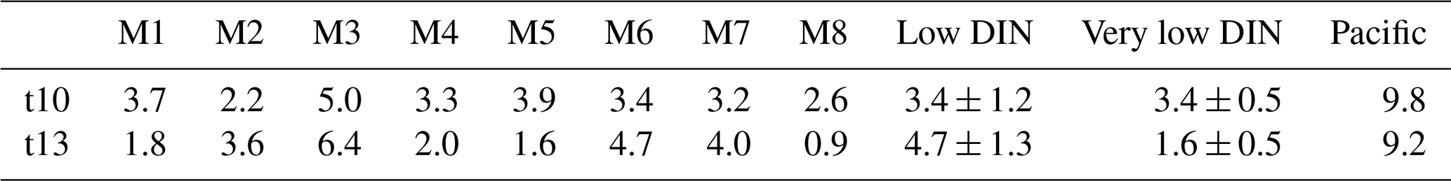
On day 10 before OMZ water addition, the average surface DIN concentrations of the two treatment groups were similar (3.4 µmol L−1) but lower than that in the Pacific (9.8 µmol L−1, Table 3). Surface layer DIN concentrations in the mesocosms ranged between 2.0 and 6.0 µmol L−1 before OMZ water addition (Fig. 2a). The addition of OMZ water elevated surface DIN in the Low DIN mesocosms to 3.6–6.4 µmol L−1 but lowered that in the Very low DIN to 0.9–2.0 µmol L−1. The average surface DIN concentration in the Very low DIN decreased to 1.6 µmol L−1 while the Low DIN slightly increased to 4.7 µmol L−1 (Table 3), followed by a sharp depletion on day 16 except for M3. M3 received the highest input of DIN (6.4 µmol L−1) and was not depleted until day 24. Despite several small peaks in M3, M4, M5, and M6 (≤1.6 µmol L−1), surface DIN concentrations in the mesocosms were at around the limits of detection (LODs – NH, 0.063 µmol L−1; NO, 0.054 µmol L−1; NO, 0.123 µmol L−1) most of the time after depletion. A slight rise could be observed from day 44 towards the last sampling day (day 48). In the Pacific, surface layer DIN concentration was mostly greater than 5 µmol L−1 (except on day 16 and 18) and became considerably higher during the second half of the experiment (> 10 µmol L−1 for day 26–44, Fig. 2a).
Table 3DIN concentration (µmol L−1) in the surface layer of each mesocosm (M1–M8) and the average DIN concentration (µmol L−1) for each treatment (Low DIN and Very low DIN; n=4) before (t10) and after deep-water addition (t13). The DIN concentration in the surface Pacific water is also shown.
Surface layer PO concentrations in the mesocosms initially ranged between 1.1 and 1.5 µmol L−1 and were elevated by OMZ water addition to around 1.9 µmol L−1 (Fig. 2b). Thereafter, PO exhibited a slow but steady decline until the end of the study with a slightly higher decrease in Low DIN mesocosms (blue symbols, Fig. 2b). Throughout the study, PO in the mesocosms was never lower than 1.1 µmol L−1. Surface layer PO in the Pacific was generally higher, fluctuating between 1.4 and 2.9 µmol L−1. In the mesocosms, enhanced chl a concentrations were observed at depths shallower than 5 m and below 15 m before OMZ water addition (Fig. 2c). Following OMZ water addition, a chl a maximum occurred at ∼ 10 m and persisted until day 40, except for M3 and M4 with a 1-week-delayed increase in the former and a lack of bloom in the latter (Fig. 2c). After day 40, chl a concentrations in all mesocosms (except for M4) increased to 12–38 µg L−1 with a bloom occurring in 0–10 m (Fig. 2c). Throughout the study, a chl a maximum was continuously observed above 10 m in the Pacific (Fig. 2c).
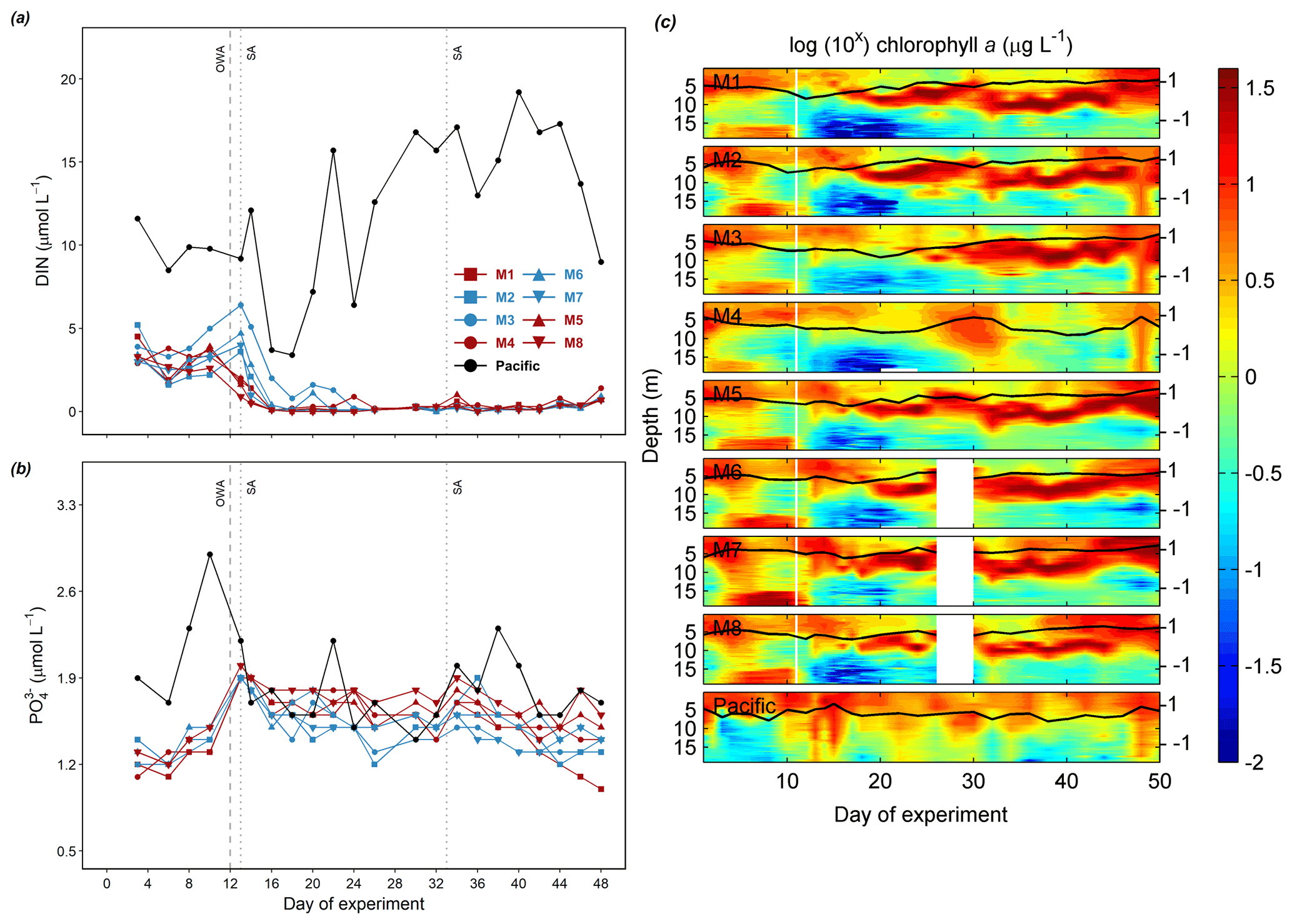
Figure 2Temporal dynamics of depth-integrated surface DIN concentration (a) and PO concentration (b) and vertical distribution of chl a concentration determined by CTD casts (c). The solid black lines on top of the colored contours represent the average values over the entire water column, with the corresponding additional y axes on the right. The vertical white lines represent the day when OMZ water was added to the mesocosms. Color codes and symbols denote the respective mesocosms. Abbreviations: OWA, OMZ water addition; SA, salt addition. The dataset is available at https://doi.pangaea.de/10.1594/PANGAEA.923395 (Bach et al., 2020b).
3.2 Temporal dynamics of carbonate chemistry
Before OMZ water addition, surface layer pHT in the mesocosms ranged between 7.80–7.94 with a slight decline by ∼ 0.1 over time (Fig. 3a). The initial surface layer TA ranged between 2310 and 2330 µmol kg−1 (Fig. 3b, day 3–12). Surface layer pCO2 and DIC ranged from 541 to 749 µatm and 2119 to 2180 µmol kg−1, respectively (Fig. 3c, d).
The two collected OMZ water masses shared similar carbonate chemistry properties despite the differences in DIN concentrations. In both water masses, pHT was ∼ 7.48, DIC was ∼ 2305–2310 µmol kg−1, TA was ∼ 2337 µmol kg−1, and pCO2 was between 1700 and 1780 µatm (Table 4).
Table 4The in situ pHT, TA, DIC, pCO2, ΩAr, and ΩCa of the two collected OMZ water masses.
Surface DIC and pCO2 were elevated from ∼ 2150 µmol kg−1 and ∼ 600 µatm to ∼ 2200 µmol kg−1 and ∼ 900 µatm (except M7), respectively, by OMZ water addition without distinct differences between the two treatments (Mann–Whitney U test, p>0.05; Fig. 3c). Following OMZ water addition, surface pCO2 in the mesocosms decreased quickly and reached minima at 340–500 µatm (except M3 and M4) on day 24 and 26. These minima corresponded with DIC minima at 2040–2110 µmol kg−1 and pHT maxima at 7.9–8.1 (except M3 and M4; Fig. 3c, d). After reaching the minima, surface layer pCO2 exhibited a steady increase to 410–680 µatm from day 24 to day 38 and later declined in M3, M5, and M7 while the rest remained relatively stable until day 42 (Fig. 3c). Interestingly, and unlike the other mesocosms, after OMZ water addition, pCO2 in M3 steadily declined from 928 to 342 µatm until the end of the experiment while that in M4 remained constantly higher than the other mesocosms (>700 µatm), with a slightly decreasing trend to 645 µatm towards the end of the study (Fig. 3c).
In the Pacific, much lower surface pHT and higher surface pCO2 and DIC were observed compared to the mesocosms, with an average of 7.7 (7.6–7.8), 1078 µatm (775–1358 µatm), and 2221 µmol kg−1 (2173–2269 µ mol kg−1; minimum-to-maximum range in parentheses; Fig. 3c, d), respectively. TA in the Pacific was initially similar to that in the mesocosms, fluctuating between 2310 and 2330 µmol kg−1, and later decreased to ∼ 2310 µmol kg−1 for the rest of the study.
Surface waters in the mesocosms and the Pacific were always saturated with respect to calcite and aragonite throughout the entire experimental period, with lower values observed in the Pacific (Fig. 4a, c). Bottom waters in the mesocosms and Pacific were always saturated with respect to calcite during the experiment (Fig. 4b), while bottom waters in the Pacific were under-saturated with respect to aragonite before day 13 (0.88–0.99) and had ΩAr values slightly above 1.0 for the rest of the study period (Fig. 4d).
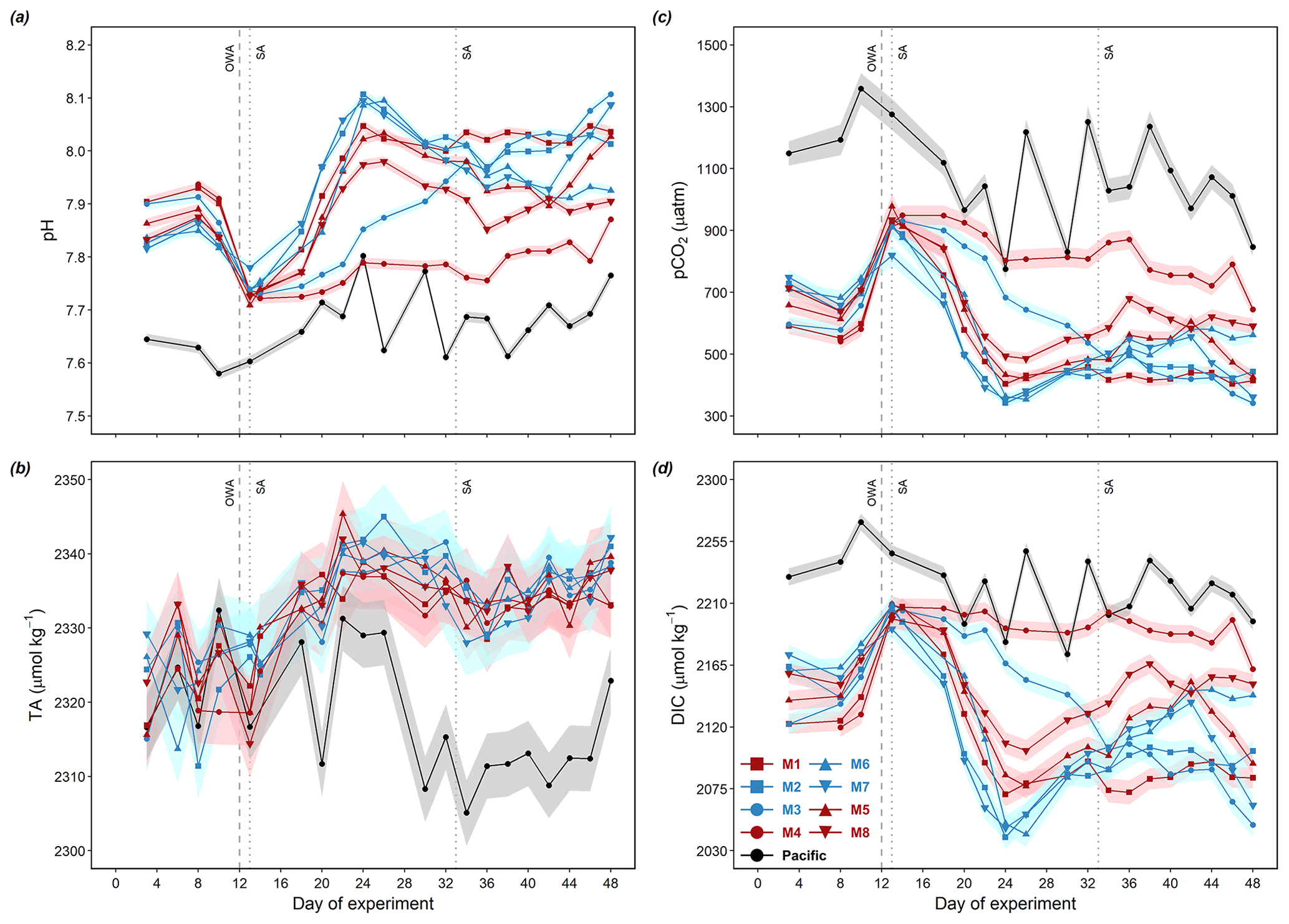
Figure 3Temporal dynamics of measured depth-integrated surface pHT (a) and TA (b) and calculated pCO2 (c) and DIC (d). The error ribbons present measurement and propagated standard uncertainties in the calculations, respectively. Color codes and symbols denote the respective mesocosms. Abbreviations: OWA, OMZ water addition; SA, salt addition.
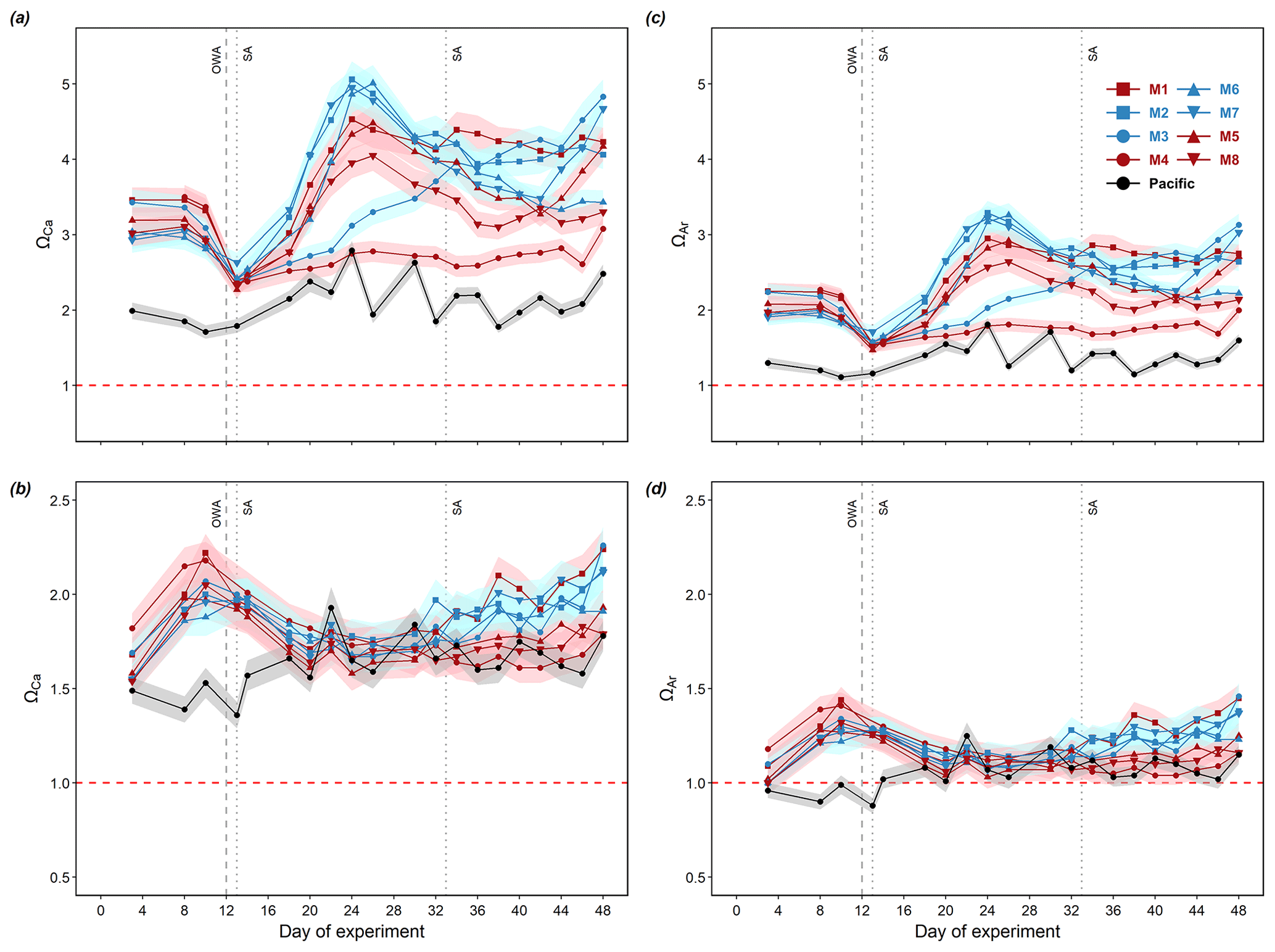
Figure 4Temporal dynamics of depth-integrated surface calcite saturation state (a), bottom calcite saturation state (b), surface aragonite saturation state (c), and bottom aragonite saturation state (d) in the mesocosms and the surrounding Pacific. The error ribbons present the propagated standard uncertainties in the calculations. When Ω>1 (above dashed red line), seawater is supersaturated for calcium carbonate. When Ω<1 (below dashed red line), seawater is under-saturated for calcium carbonate. Color codes and symbols denote the respective mesocosms. Abbreviations: OWA, OMZ water addition; SA, salt addition.
3.3 Air–sea CO2 fluxes in the Pacific
Positive FCO2 values indicate CO2 outgassing from the surface waters to the atmosphere, while negative values indicate a CO2 flux from the atmosphere to the ocean. The air–sea CO2 flux in the Pacific was constantly positive throughout our study, fluctuating from 4.2 to 14.0 mmol C m−2 d−1 over time (Fig. 5a). The minima of FCO2 occurred on day 26 and 30, while the maximum occurred on day 32 when near-surface wind was the highest (2.89 m s−1, Fig. 5b), corresponding to the minima and maxima of surface pCO2. Co-occurring with a decrease in surface temperature to below 19 ∘C after day 36 (Fig. 5c), FCO2 slightly declined from ∼ 10 to ∼ 6 mmol C m−2 d−1 (Fig. 5a). FCO2 was positively correlated with near-surface wind speed (r2=0.4). No correlation was found between FCO2 and temperature (r2=0).
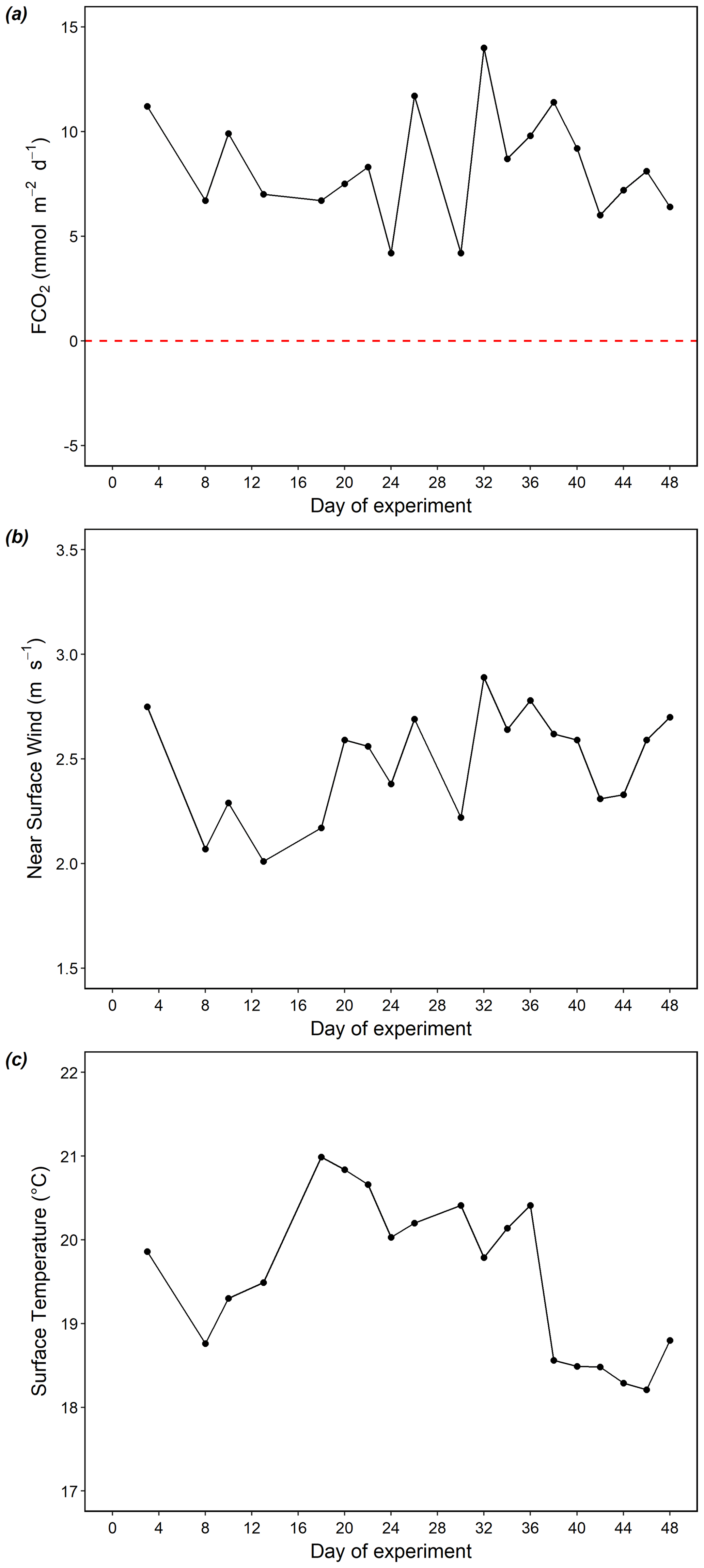
Figure 5Temporal dynamics of surface air–sea CO2 flux (a), near-surface wind speed (b), and surface temperature (c) in the Pacific. FCO2>0 (above dashed red line) indicates CO2 outgassing from the sea surface to the atmosphere. FCO2<0 (below dashed red line) indicates a CO2 flux from the atmosphere to the sea.
4.1 Quality control and propagated uncertainties
To compare the sensitivity of different calculated variables to uncertainties in the input variables, the propagated uncertainties were averaged for each calculated variable, reported in numerical values and percentages relative to the calculated values of each variable (Table 1). Among the 4 reported variables, ΩCa and ΩAr were the most sensitive to uncertainties in pHT and TA with an average uncertainty of 5.1 %. This adds ambiguity to whether the bottom water (10–17 m for day 3–28, 12.5–17 m for day 29–50) in the Pacific was under-saturated with respect to aragonite when ΩAr was oscillating near 1 (Fig. 4d). The propagated uncertainty in pCO2 was slightly lower (3.8 %), while DIC was the least sensitive (0.3 %).
We examined the internal consistency between DIC measurements and calculations. DIC was measured from day 3 until the malfunction of the instrument on day 10. In total, 53 sets of measured DIC and calculated DIC (from measured pHT and TA) values were obtained from day 3 to day 10 and compared to test their consistency (Fig. 6a). The calculated DIC values were generally in agreement with the measured values (r2=0.985; p<0.005), showing that the calculations made an overall good prediction for the measured DIC values. The average of the residuals (calculated DIC − measured DIC) was −8.27 ± 6.9 µmol kg−1, indicating an underestimation of calculated DIC. This result is consistent with a previous observation of underestimated calculated DIC (pHT, TA) compared with measured DIC when applying the same set of constants (−6.6 ± 7.9 µmol kg−1; Raimondi et al., 2019). The reasons for such underestimation have not been addressed in previous studies and remain unclear. No significant relationships with input variables pHT and TA (r2=0.12 for both) and temperature (r2=0.30) were found in the DIC residuals (salinity remained the same from day 3 to day 10). The lack of correlation with pHT and TA indicated that the underestimation in calculated DIC was not a result from changes in pHT and TA. Although dissociation constants are known to be salinity- and temperature-dependent, the lack of correlation between DIC residuals and temperature may be attributed to the relatively narrow ranges of temperature in the mesocosms (17.9–20.9 ∘C from day 3–10). The offsets were typically larger at lower temperatures (e.g., samples from the Arctic; Chen et al., 2015).
To assess the quality of carbonate chemistry measurements in this study, the stability and performance of measurements were evaluated. The standard deviation of triplicate pHT measurements varied by up to 0.003 with an average of 0.0012 throughout the whole experiment (Fig. 6b). The average standard deviation was in agreement with reported analytical precisions of pH (0.003, Orr et al., 2018; 0.002, Raimondi et al., 2019; Ma et al., 2019).
For TA, triplicate measurements of CRM distributed before and after the sample measurements were carried out on each measuring day to monitor the stability of the measurement process and the performance of the system. Based on the offsets, a correction factor was applied to the measured values of samples on each sampling day to calibrate for instrument drift. As shown in Fig. 6c, 90.5 % of the measured TA values of CRM fell between warning limits (upper warning limit, UWL, and lower warming limit, LWL) with one data point falling outside the control limits (upper control limit, UCL, and lower control limit, LCL), overall suggesting a relatively stable measurement system. The average measured TA was 2209.9 µmol kg−1, which was 17.69 µmol kg−1 lower than the certified concentration of the CRM (2227.59 µmol kg−1), indicating a relatively poor accuracy (compared to the suggested bias of less than 2 µmol kg−1; Dickson et al., 2003, 2007). The poor accuracy could be attributed to the fact that the concentration of the acid titrant was not checked after being prepared, as suggested in the protocol (Dickson et al., 2003). A range control chart was computed based on duplicate measurements of CRM made prior to the sample measurements on each sampling day to evaluate the consistency of the offset between measured and certified TA values over the course of the study (Fig. 6d; Dickson et al., 2007). The absolute difference (range) between the repeated CRM measurements was on average 1.4 µmol kg−1. All the range values fell below the UWL (3.50 µmol kg−1, Fig. 6d), suggesting a relatively good precision of the measurement system.
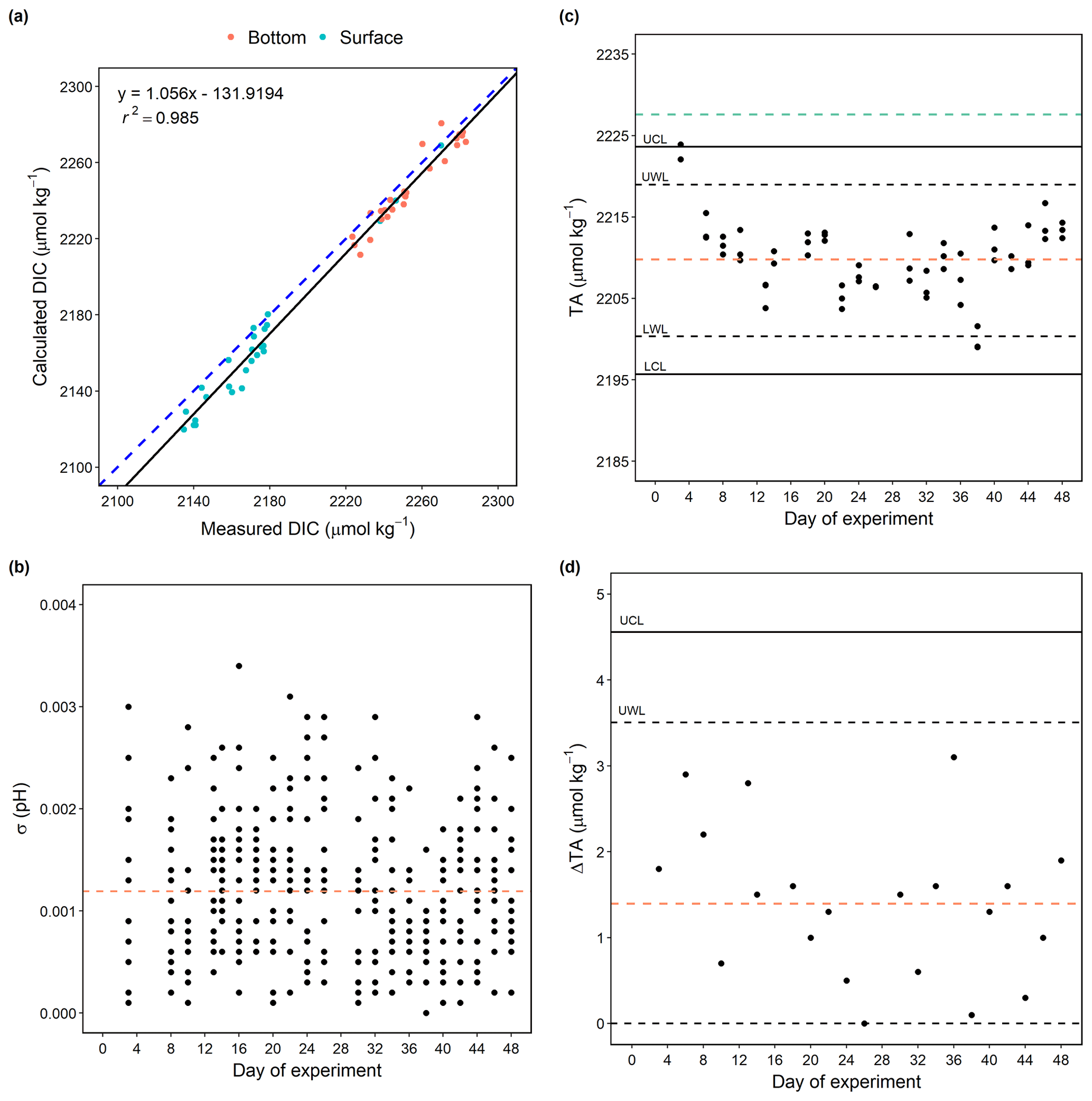
Figure 6Comparison of calculated values of DIC (pHT, TA) and measured values (a). The black line is the regression line, with the corresponding equation and r2 shown in the top-left corner. The dashed blue line shows the regression line forced through the origin. Standard deviations are of all the triplicate pHT measurements on each sampling day over the study period. The dashed orange line shows the average (n=377) of the standard deviations (b). TA values of CRM measurements on each sampling day over the study period. The dashed orange line shows the average (n=62) of the measured values, and the dashed green line indicates the certified value of the CRM (c). The absolute difference in TA values between duplicate CRM measurements (range) on each sampling day over the study period. The dashed orange line shows the average (n=21) of the ranges (d). Abbreviations: UCL, upper control limit; UWL, upper warning limit; LWL, lower warning limit; LCL, lower control limit.
4.2 CO2 responses to the simulated upwelling event
At the beginning of the experiment, surface pCO2 levels in the mesocosms were > 500 µatm (Fig. 3c). This suggests that we initially enclosed an upwelled water mass that was enriched with respiratory CO2. The addition of OMZ water with high concentrations of CO2 to the mesocosms reduced the surface pHT by 0.1–0.2 and increased the surface pCO2 to > 900 µatm (except for M7, which was 819.4 µatm on day 13). The simulated upwelling substantially reduced the variability in CO2 between mesocosms because OMZ water addition replaced ∼ 20 m3 of seawater in each mesocosm (out of ∼ 54 m3). The enhanced pCO2 level is comparable with our observations in the ambient Pacific water (> 775 µatm, Fig. 3c). These values also agree with reported observations for our study area in 2013 (> 1200 µatm in the upper 100 m and > 800 µatm at the surface; Bates, 2018).
In the days after OMZ water addition, surface pCO2 in the mesocosms dropped near or below the atmospheric level (405.22 µatm; Dlugokencky and Tans, 2021; NOAA/GML) with a decline in DIC by ∼ 100 µmol kg−1 (except M3 and M4; Fig. 3c, d). The declining pCO2 could be partially attributed by CO2 outgassing due to a high CO2 gradient from the sea surface to the air. Due to a rare coastal El Niño event (Garreaud, 2018), the CO2 loss process may have been enhanced by a rapid surface warming (19.8–21.0 ∘C from day 14 to 36, Fig. 5) which reduced surface CO2 solubility (Zeebe and Wolf-Gladrow, 2001). However, air–sea gas exchange could not explain surface CO2 under-saturation in relation to the atmosphere, as observed in response to OMZ water addition in some mesocosms (Van Geen et al., 2000; Friederich et al., 2008; Fig. 3c). Biological production typically has impacts on CO2 drawdown that are 1 to 4 times greater than air–sea gas exchange in the equatorial Pacific where surface waters are exposed to local wind stress (Feely et al., 2002). This interpretation is supported by the continuously high DIC in M4 where photosynthetic biomass buildup was substantially lower (Fig. 3d). Hence, the depletion of nutrients (Fig. 2a, b) and increase in chl a concentration (Fig. 2c; Bach et al., 2020a) strongly suggest that the loss of DIC (except M4) was primarily driven by biological uptake and phytoplankton growth. Nevertheless, it is difficult to dissect how much CO2 was outgassed and how much was taken up photosynthetically as we did not measure air–sea gas exchange in the mesocosms (please note that equations from Wanninkhof, 2014, are not applicable to mesocosms; Czerny et al., 2013b). In previous mesocosm studies, N2O addition has been a common practice to monitor air–sea gas exchange in the mesocosms (Czerny et al., 2013b). However, this was not carried out in our study because it would have interfered with 15N label incubations to determine N loss processes (Schulz et al., 2021). Due to high variability in DOC data and the poorly constrained gas exchange of CO2, C budgeting often comes with high uncertainties and large errors, even for a relatively simple dataset (Czerny et al., 2013b; Boxhammer et al., 2018). It becomes even more difficult for the current dataset because the water column was not homogeneously mixed like in previous studies. With the inability to estimate CO2 gas exchange, it was impossible to calculate a reasonable C budget for this study. Before OMZ water addition, dissolved inorganic N:P ratios in the mesocosms ranged from 1.6 to 3.5 (data not shown), indicating N is the limiting nutrient in the water column (Bach et al., 2020a). Not surprisingly, the uptake of DIC was higher in the Low DIN mesocosms, which received more input of DIN from OMZ water addition, with on average 41.0 µmol kg−1 higher drawdown compared to the Very low DIN from day 13 to day 24 (excluding M3 and M4; Mann–Whitney U test, p=0.05; Table S1). This observation agrees with the general expectations that the addition of limiting nutrients to the water column should enhance biological biomass buildup. Such differences in DIC uptake, however, were not reflected in the buildup of particulate organic carbon (POC) in the mesocosms (excluding M3 and M4; Mann–Whitney U test, p>0.1). As mentioned above, the differences in OMZ water DIN between the two treatments were minor, and hence, their potential to trigger treatment differences was small. Also, Akashiwo sanguinea was persistent in the water column in the mesocosms (except M4 where it never bloomed), retaining the biomass in the water column and not sinking out until the very end of the experiment (Bach et al., 2020a). Due to the developing N limitation after the biomass buildup there, much of the consumed DIC could have been channeled to the dissolved organic carbon (DOC) pool. Indeed, we observed a pronounced increase in DOC following OMZ water addition (except for M4; Igarza et al., 2022). The increase in DOC may be attributed to extracellular release by phytoplankton due to nutrient limitation or cellular lysis of phytoplankton cells by bacteria (Myklestad, 2000; Igarza et al., 2022).
After day 24, variability in carbonate chemistry between individual mesocosms increased, with a general trend of recovering from CO2-under-saturated conditions during the peak of the bloom (except for M3 and M4, Fig. 3c). One factor that may have controlled the differences in CO2 increase are the mesocosm-specific phytoplankton succession patterns. A shift from a diatom-dominated community to a dominance of dinoflagellates (in particular Akashiwo sanguinea) occurred when DIN was exhausted, which was absent in M3 and M4 (Bach et al., 2020a). The different succession patterns in the plankton community are the most likely explanation of why M3 and M4 behaved differently from the others in terms of surface layer productivity and hence carbonate chemistry. Although the rates of DIN depletion in M3 and M4 were similar to the others, the reduction in pCO2 in M3 experienced a 1-week delay, which is consistent with the delayed buildup of chl a biomass (Figs. 2c, 3c). On the other hand, the pCO2 level in M4 remained constantly elevated throughout the experiment, indicative of a lack of a phytoplankton bloom (Figs. 2c, 3c). M4 was the only mesocosm where A. sanguinea remained undetectable, whereas a delayed and reduced contribution by A. sanguinea was observed in M3. This strongly suggests that A. sanguinea was a key factor driving the trend of carbonate chemistry in the mesocosms.
Near the end of the experiment, a slight decline in pCO2 became apparent in the mesocosms, which co-occurred with a second phytoplankton bloom observed in the uppermost layer of the water column (Figs. 2c, 3c). This bloom was likely fueled by surface eutrophication due to defecating sea birds. During the last part of our experiment, Inca terns (Larosterna inca) were frequently observed to rest on the roofs and the edges of the mesocosms (Bach et al., 2020a). Bird excrements, dropped into the mesocosms, are known to be enriched in inorganic nutrients (Bedard et al., 1980). They generally contain 60 % water, 7.3 % N and, 1.5 % P, and the main form of N is uric acid and ammonium, which makes them slightly acidic (De La Peña-Lastra, 2021). Therefore, the droppings may lower the pH of the surface water. However, this should have been visible in decreasing alkalinity, which was not the case. The excrements may also be high in dissolved organic nitrogen (DON), evidenced by a substantial increase in DON concentrations in the mesocosm surface from day 38 onward (Igarza et al., 2022). The triggered surface eutrophication and phytoplankton blooms were noticeable from an accumulation of chl a biomass above the mixed layer in the mesocosms near the end of the study (Fig. 2c). As a result, another drawdown of DIC could be observed in the mesocosms except for M4, M6, and M8. While the buildup of chl a was comparable with that triggered by OMZ water addition, the drawdown in DIC was less pronounced, potentially counteracted by the release of CO2 by enhanced respiration and remineralization following the previous bloom. Also, the second bloom occurred in the top 2 meter in the mesocosms (Fig. 2c), where gas exchange can quickly replete the DIC drawdown during photosynthesis and biomass build up.
There are potential complications when monitoring the carbonate chemistry dynamics in an enclosed mesocosm. First, the brine addition to the mesocosms could have influenced the community composition which played an important role in driving the carbonate chemistry. However, the effects of the brine on the enclosed organisms have been discussed in past studies and considered negligible for a salinity increase of less than 1 (∼ 0.7 and ∼ 0.5 increase for both salt additions in our study, respectively; Czerny et al., 2013a). The difference in salinity in the mesocosms from the Pacific was less than 1 throughout the study, so we believe salinity was not a stressor to the system (Bach et al., 2020a). Second, multiple factors may introduce variabilities into air–sea gas exchange in the mesocosms. With the water surface sheltered from direct wind forcing by the 2 m high plastic walls of the mesocosm bag, air–sea gas exchange could be very low (but not zero due to other energy inputs such as thermal convection and surrounding wave movements; Czerny et al., 2013b). On the other hand, the extensive daily sampling that actively perturbs the mesocosm surface may enhance the gas exchange (Czerny et al., 2013b). With a high variability in DOC data and a lack of direct measurements of CO2 gas exchange, it is impossible to estimate a reasonable C budget for our dataset (Czerny et al., 2013b; Boxhammer et al., 2018). Other complications include heterogenous initial conditions in the mesocosms and light limitation due to self-shading (please see Bach et al., 2020a, for an extensive discussion). It would have been ideal to have had control mesocosms that were treated the same way except in terms of the OMZ water addition to rule out the effects induced by mesocosm manipulations and changes in hydrodynamics. Not having this was a compromise to ensure enough replicate numbers for both treatments despite the enormous cost of mesocosm experimentation. Nevertheless, a previous study has examined impacts of different mixing techniques in outdoor mesocosms and found no effects on phytoplankton biomass and minor effects on phytoplankton and zooplankton community composition (Striebel et al., 2013). In our study, various measures were also taken to minimize the mixing (brine additions and slow casting of CTD).
4.3 Temporal changes in carbonate chemistry in the coastal Pacific near Callao
According to estimations by Takahashi et al. (2009) of global air–sea CO2 fluxes, our study site in the equatorial Pacific (14∘ N–14∘ S) is a major source of CO2 to the atmosphere. Our near-coastal location showed high pCO2 levels over the study period (with an average of 1078 µatm), with a sea-to-air CO2 flux of 4.2–14.0 mmol C m−2 d−1 (Fig. 5). Compared to the criterion of high CO2 fluxes (5 mmol C m−2 d−1 or more) as proposed by Paulmier et al. (2008), our study site was a strong CO2 source to the atmosphere most of the time. These results of air–sea CO2 fluxes were slightly higher than observations by Friederich et al. (2008) along the coast of Peru in February 2004–2006 (0.85–4.54 mol C m−2 yr−1, spatially averaged for 5–15∘ S along the coast of Peru). This is not surprising because Friederich et al. (2008) averaged the air–sea CO2 fluxes for 0–200 km from the shore, where much lower pCO2 levels were observed offshore (< 600 µatm) compared to our nearshore study site. The decline in pCO2 with increasing distance from shore was driven by biological uptake and outgassing to the atmosphere (Friederich et al., 2008; Loucaides et al., 2012). However, when compared to the magnitude of DIC drawdown triggered by upwelling events in the mesocosms, the flux of CO2 to the atmosphere was insignificant. Assuming a 10 m mixed layer in the Pacific with a DIC concentration of 2200 µmol kg−1, the DIC content below a 1 m2 surface area would be ∼ 22 mol m−2. With an upper bound outgassing of 14.2 mmol C m−2 d−1 over 10 d (day 13–24), the loss of CO2 would only be 0.142 mol m−2. On the other hand, the average DIC drawdown of 118.2 µmol kg−1 in the Very low DIN and 160.3 µmol kg−1 in the Low DIN mesocosms (M3 and M4 excluded) during this period accounts for 1.18 and 1.60 mol m−2, respectively, over the same water column. This shows that biological processes drawing down CO2 are stronger than loss by air–sea gas exchange.
During our study, we experienced a coastal El Niño event which was the strongest on record (compared to those recorded in 1891 and 1925) and induced rapid sea surface warming of ∼ 1.5 ∘C and enhanced stratification (Garreaud, 2018). Previous investigations showed that the impact of reduced upwelling on CO2 fluxes is pronounced for upwelling areas (Feely et al., 1999, 2002). A decline in upwelling of CO2-enriched OMZ water results in a decrease in sea-to-air CO2 fluxes. For example, during the 1991–1994 El Niño year, a total reduction in CO2 fluxes to the atmosphere was reported for the equatorial Pacific. They were only 30 %–80 % of that of a non-El Niño year (Feely et al., 1999, 2002). This is likely to be the case for our study location. Most studies have investigated air–sea CO2 fluxes at larger timescales and regional scales (Feely et al., 1999; Friederich et al., 2008; Takahashi et al., 2009). Therefore, it is difficult to conclude the magnitude of the coastal El Niño influence on the local CO2 fluxes in our study by comparing our results with previous observations. Nevertheless, our observations can serve as the first evidence of carbonate chemistry dynamics in the coastal Peruvian upwelling system during a coastal El Niño event. Observations of sea surface carbonate chemistry with a high temporal resolution (every second day) in nearshore waters are scarce, as they are rarely covered by typical research expeditions in the open ocean (Takahashi et al., 2009; Franco et al., 2014), especially during such an extremely rare coastal El Niño event. Comparisons of our data with previous or future observations may enhance our understanding of how inorganic carbon cycling interacts with extreme climate events in upwelling systems.
CO2-enriched OMZ water has been occasionally reported to be under-saturated with respect to aragonite (Feely et al., 2008; Fassbender et al., 2011). In our study, calcite under-saturation did not occur in the mesocosms or in the Pacific (Fig. 4). Aragonite under-saturation, however, was observed below the surface (10–17 m for day 3–28, 12.5–17 m for day 29–50) of the Pacific at the start of the experiment (Fig. 4d), when pCO2 was the highest (pCO2>1100 µatm, Fig. 3c). Aragonite under-saturation was also observed in the two deep water masses collected at deeper depths (30 and 70 m) in the Pacific (Table 4). Throughout the study period, the aragonite saturation state fluctuated close to around 1 below the surface (Fig. 4d). Considering the water column we sampled in the Pacific still belonged to the upper surface ocean, we could expect deeper and more CO2-enriched water in the underlying OMZ to be most likely under-saturated with respect to calcite and aragonite. Hence, our observations of aragonite under-saturation in the Pacific suggest a potential risk of dissolution for marine calcifiers in response to the ongoing intensification and expansion of acidified OMZ water (Comeau et al., 2009; Lischka et al., 2011; Maas et al., 2012).
Our observations in the mesocosms revealed that, following the addition of two OMZ water masses with different nutrient signatures, there was a higher drawdown of DIC in response to slightly more DIN input from the OMZ water addition but no difference in the buildup of POC and chl a (Figs. 2a and c, 3d). The timing of the first phytoplankton bloom was consistent with a shift from a diatom-dominated community to A. sanguinea dominance in most mesocosms, indicating that A. sanguinea was a key factor driving the changes in carbonate chemistry under N-limited conditions. A second phytoplankton bloom was triggered by defecation of Inca terns, which eased the N limitation in the mesocosms (Fig. 2c). These findings provide improved insights into the links between upwelling-induced N limitation, phytoplankton community shifts, and carbonate chemistry dynamics in the Peruvian upwelling system.
The surrounding Pacific waters at the study site were characterized by constantly high pCO2 levels (with an average of 1078.1 µatm). Most CO2 flux estimates have been conducted in the open ocean, and few studies have surveyed coastal regions (Takahashi et al., 2009; Franco et al., 2014). Our study site was a strong CO2 source to the atmosphere most of the time (4.2–14.2 mmol C m−2 d−1), despite a rare coastal El Niño event. However, evidence from our mesocosm experiment suggests biological responses that draw down DIC can quickly turn a CO2 source into a sink in the upwelling system. The influence of the co-occurring coastal El Niño event on the local CO2 fluxes remains unclear. Nevertheless, future carbonate chemistry fluctuations are expected to be enhanced by expanding and intensifying ocean deoxygenation, as well as by reducing buffer factors (Schulz et al., 2019). Hence, it is essential to improve our understanding of the mechanisms driving the inorganic carbon cycling in upwelling systems. As a unique dataset that characterized nearshore carbonate chemistry with a high temporal resolution during a rare coastal El Niño event, our study gives important insights into the carbonate chemistry responses to extreme climate events in the Peruvian upwelling system.
The dataset is now available under https://doi.org/10.1594/PANGAEA.933337 (Chen et al., 2021) and https://doi.pangaea.de/10.1594/PANGAEA.923395 (Bach et al., 2020b).
The supplement related to this article is available online at: https://doi.org/10.5194/bg-19-295-2022-supplement.
UR, KGS, and LTB designed the experiment. All authors contributed to the sampling. SMC measured, calculated, and analyzed the carbonate chemistry. LTB and KGS supervised the carbonate chemistry analysis. KGS carried out the CTD casts and data analyses. EvdE and EPA measured and analyzed nutrients. SMC wrote the manuscript with input from all the co-authors.
The contact author has declared that neither they nor their co-authors have any competing interests.
Publisher's note: Copernicus Publications remains neutral with regard to jurisdictional claims in published maps and institutional affiliations.
This article is part of the special issue “Ecological and biogeochemical functioning of the coastal upwelling system off Peru: an in situ mesocosm study”. It is not associated with a conference.
This project was supported by the Collaborative Research Center SFB 754 Climate-Biogeochemistry Interactions in the Tropical Ocean financed by the German Research Foundation (DFG). Additional funding was provided by the EU project AQUACOSM and the Leibniz Prize 2012 granted to Ulf Riebesell. We thank all participants of the KOSMOS Peru 2017 experiment for mesocosm maintenance and sample collection and analysis. Special thanks go to the staff of IMARPE; the captains and crews of BAP Morales, IMARPE VI, and BIC Humboldt; and Marina de Guerra del Perú, in particular the submarine section of the navy of Callao, and the Dirección General de Capitanías y Guardacostas for their support and assistance in planning and carrying out the experiment. We are thankful to Club Náutico Del Centro Naval for hosting our laboratories, office space, and support. This work is a contribution in the framework of the cooperation agreement between IMARPE and GEOMAR through the German Federal Ministry for Education and Research (BMBF) project ASLAEL 12-016 and the national project Integrated Study of the Upwelling System off Peru developed by the Direction of Oceanography and Climate Change of IMARPE, PPR 137 CONCYTEC. Analyses and visualizations used in this paper were produced with the Giovanni online data system, developed and maintained by the NASA GES DISC.
This research has been supported by the Collaborative Research Center SFB 754 Climate-Biogeochemistry Interactions in the Tropical Ocean financed by the German Research Foundation (DFG), the EU project AQUACOSM, and the Leibniz Award 2012 (granted to Ulf Riebesell).The article processing charges for this open-access publication were covered by the GEOMAR Helmholtz Centre for Ocean Research Kiel.
This paper was edited by Hans-Peter Grossart and reviewed by two anonymous referees.
Albert, A., Echevin, V., Lévy, M., and Aumont, O.: Impact of nearshore wind stress curl on coastal circulation and primary productivity in the Peru upwelling system, J. Geophys. Res.-Oceans, 115, https://doi.org/10.1029/2010JC006569, 2010.
Bach, L. T., Boxhammer, T., Larsen, A., Hildebrandt, N., Schulz, K. G., and Riebesell, U.: Influence of plankton community structure on the sinking velocity of marine aggregates, Global Biogeochem. Cy., 30, 1145–1165, 2016.
Bach, L. T., Paul, A. J., Boxhammer, T., von der Esch, E., Graco, M., Schulz, K. G., Achterberg, E., Aguayo, P., Arístegui, J., Ayón, P., Baños, I., Bernales, A., Boegeholz, A. S., Chavez, F., Chavez, G., Chen, S.-M., Doering, K., Filella, A., Fischer, M., Grasse, P., Haunost, M., Hennke, J., Hernández-Hernández, N., Hopwood, M., Igarza, M., Kalter, V., Kittu, L., Kohnert, P., Ledesma, J., Lieberum, C., Lischka, S., Löscher, C., Ludwig, A., Mendoza, U., Meyer, J., Meyer, J., Minutolo, F., Ortiz Cortes, J., Piiparinen, J., Sforna, C., Spilling, K., Sanchez, S., Spisla, C., Sswat, M., Zavala Moreira, M., and Riebesell, U.: Factors controlling plankton community production, export flux, and particulate matter stoichiometry in the coastal upwelling system off Peru, Biogeosciences, 17, 4831–4852, https://doi.org/10.5194/bg-17-4831-2020, 2020a.
Bach, L. T., Paul, A. J., Boxhammer, T., von der Esch, E., Graco, M., Schulz, K. G., Achterberg, E., Aguayo, P., Arístegui, J., Ayón, P., Baños, I., Bernales, A., Boegeholz, A. S., Chavez, F., et al.: KOSMOS 2017 Peru mesocosm study: overview data, [data set], https://doi.org/10.1594/PANGAEA.923395, 2020b.
Bakun, A. and Weeks, S. J.: The marine ecosystem off Peru: What are the secrets of its fishery productivity and what might its future hold?, Prog. Oceanogr., 79, 290–299, https://doi.org/10.1016/j.pocean.2008.10.027, 2008.
Bates, N. R.: Seawater carbonate chemistry distributions across the Eastern South Pacific Ocean sampled as part of the GEOTRACES project and changes in marine carbonate chemistry over the past 20 years, Front Mar. Sci., 5, 1–18, https://doi.org/10.3389/fmars.2018.00398, 2018.
Beaudoing, H. and Rodell, M.: NASA/GSFC/HSL: GLDAS Noah Land Surface Model L4 3 hourly 0.25 x 0.25 degree V2.1, Greenbelt, Maryland, USA, Goddard Earth Sciences Data and Information Services Center (GES DISC), https://doi.org/10.5067/E7TYRXPJKWOQ, 2020.
Bedard, J., Therriault, J. C., and Berube, J.: Assessment of the importance of nutrient recycling by seabirds in the St. Lawrence Estuary, Can. J. Fish. Aquat. Sci., 37, 583–588, https://doi.org/10.1139/f80-074, 1980.
Bockmon, E. E. and Dickson, A. G.: A seawater filtration method suitable for total dissolved inorganic carbon and pH analyses, Limnol. Oceanogr.-Meth., 12, 191–195, https://doi.org/10.4319/lom.2014.12.191, 2014.
Bopp, L., Resplandy, L., Orr, J. C., Doney, S. C., Dunne, J. P., Gehlen, M., Halloran, P., Heinze, C., Ilyina, T., Séférian, R., Tjiputra, J., and Vichi, M.: Multiple stressors of ocean ecosystems in the 21st century: projections with CMIP5 models, Biogeosciences, 10, 6225–6245, https://doi.org/10.5194/bg-10-6225-2013, 2013.
Capone, D. G. and Hutchins, D. A.: Microbial biogeochemistry of coastal upwelling regimes in a changing ocean, Nat. Geosci., 6, 711, https://doi.org/10.1038/ngeo1916, 2013.
Carter, B. R., Radich, J. A., Doyle, H. L., and Dickson, A. G.: An automated system for spectrophotometric seawater pH measurements, Limnol. Oceanogr.-Meth., 11, 16–27, https://doi.org/10.4319/lom.2013.11.16, 2013.
Chavez, F. P. and Messié, M.: A comparison of eastern boundary upwelling ecosystems, Prog. Oceanogr., 83, 80–96, https://doi.org/10.1016/j.pocean.2009.07.032, 2009.
Chavez, F. P., Bertrand, A., Guevara-Carrasco, R., Soler, P., and Csirke, J.: The northern Humboldt Current System: Brief history, present status and a view towards the future, Prog. Oceanogr., 79, 95–105, https://doi.org/10.1016/j.pocean.2008.10.012, 2008.
Chen, B., Cai, W. J., and Chen, L.: The marine carbonate system of the Arctic Ocean: assessment of internal consistency and sampling considerations, summer 2010, Mar. Chem., 176, 174–188, https://doi.org/10.1016/j.marchem.2015.09.007, 2015.
Chen, S.-M., Riebesell, U., Schulz, K. G., von der Esch, E., Achterberg, E. P., and Bach, L. T.: KOSMOS 2017 Peru mesocosm study: carbonate chemistry data, PANGAEA [data set], https://doi.org/10.1594/PANGAEA.933337, 2021.
Clayton, T. D. and Byrne, R. H.: Spectrophotometric seawater pH measurements: total hydrogen ion concentration scale calibration of m-cresol purple and at-sea results, Deep Sea Res. Pt. I, 40, 2115–2129, https://doi.org/10.1016/0967-0637(93)90048-8, 1993.
Comeau, S., Gorsky, G., Jeffree, R., Teyssié, J.-L., and Gattuso, J.-P.: Impact of ocean acidification on a key Arctic pelagic mollusc (Limacina helicina), Biogeosciences, 6, 1877–1882, https://doi.org/10.5194/bg-6-1877-2009, 2009.
Coverly, S., Kérouel, R., and Aminot, A.: A re-examination of matrix effects in the segmented-flow analysis of nutrients in sea and estuarine water, Anal. Chim. Acta, 712, 94–100, 2012.
Czerny, J., Schulz, K. G., Krug, S. A., Ludwig, A., and Riebesell, U.: Technical Note: The determination of enclosed water volume in large flexible-wall mesocosms “KOSMOS”, Biogeosciences, 10, 1937–1941, https://doi.org/10.5194/bg-10-1937-2013, 2013a.
Czerny, J., Schulz, K. G., Ludwig, A., and Riebesell, U.: Technical Note: A simple method for air–sea gas exchange measurements in mesocosms and its application in carbon budgeting, Biogeosciences, 10, 1379–1390, https://doi.org/10.5194/bg-10-1379-2013, 2013b.
Dale, A. W., Sommer, S., Lomnitz, U., Montes, I., Treude, T., Liebetrau, V., Gier, J., Hensen, C., Dengler, M., Stolpovsky, K., Bryant, L. D., and Wallmann, K.: Organic carbon production, mineralisation and preservation on the Peruvian margin, Biogeosciences, 12, 1537–1559, https://doi.org/10.5194/bg-12-1537-2015, 2015.
Deutsch, C., Gruber, N., Key, R. M., Sarmiento, J. L., and Ganachaud, A.: Denitrification and N2 fixation in the Pacific Ocean, Global Biogeochem. Cy., 15, 483–506, https://doi.org/10.1029/2000GB001291, 2001.
Deutsch, C., Sarmiento, J. L., Sigman, D. M., Gruber, N., and Dunne, J. P.: Spatial coupling of nitrogen inputs and losses in the ocean, Nature, 445, 163–167, https://doi.org/10.1038/nature05392, 2007.
Dickson, A. G.: Standards for ocean measurements, Oceanogr., 23, 34–47, doi10.5670/oceanog.2010.22, 2010.
Dickson, A. G., Wesolowski, D. J., Palmer, D. A., and Mesmer, R. E.: Dissociation constant of bisulfate ion in aqueous sodium chloride solutions to 250 ∘C, J. Phys. Chem., 94, 7978–7985, https://doi.org/10.1021/j100383a042, 1990.
Dickson, A. G., Afghan, J. D., and Anderson, G. C.: Reference materials for oceanic CO2 analysis: a method for the certification of total alkalinity, Mar. Chem., 80, 185–197, https://doi.org/10.1016/S0304-4203(02)00133-0, 2003.
Dickson, A. G., Sabine, C. L., and Christian, J. R. (Eds.): Guide to Best Practices for Ocean CO2 Measurements, PICES Special Publication 3, 191 pp., 2007.
Dlugokencky, E. and Tans, P.: NOAA/GML, available at: https://gml.noaa.gov/ccgg/trends/, last access: 6 April 2021.
Doney, S. C., Ruckelshaus, M., Duffy, J. E., Barry, J. P., Chan, F., English, C. A., Galindo, H. M., Grebmeier, J. M., Hollowed, A. B., Knowlton, N., and Polovina, J.: Climate change impacts on marine ecosystems, Ann. Rev. Mar. Sci., 4, 11–37, https://doi.org/10.1146/annurev-marine-041911-111611, 2012.
Douglas, N. K. and Byrne, R. H.: Achieving accurate spectrophotometric pH measurements using unpurified meta-cresol purple, Mar. Chem., 190, 66–72, 2017.
Echevin, V., Aumont, O., Ledesma, J., and Flores, G.: The seasonal cycle of surface chlorophyll in the Peruvian upwelling system: A modelling study, Prog. Oceanogr., 79, 167–176, https://doi.org/10.1016/j.pocean.2008.10.026, 2008.
Fassbender, A. J., Sabine, C. L., Feely, R. A., Langdon, C., and Mordy, C. W.: Inorganic carbon dynamics during northern California coastal upwelling, Cont. Shelf Res., 31, 1180–1192, https://doi.org/10.1016/j.csr.2011.04.006, 2011.
Fassbender, A. J., Sabine, C. L., and Feifel, K. M.: Consideration of coastal carbonate chemistry in understanding biological calcification, Geophys. Res. Lett., 43, 4467–4476, https://doi.org/10.1002/2016GL068860, 2016.
Feely, R. A., Wanninkhof, R., Takahashi, T., and Tans, P.: Influence of El Niño on the equatorial Pacific contribution to atmospheric CO2 accumulation, Nature, 398, 597–601, https://doi.org/10.1038/19273, 1999.
Feely, R. A., Sabine, C. L., Hernandez-Ayon, J. M., Ianson, D., and Hales, B.: Evidence for upwelling of corrosive “acidified” water onto the continental shelf, Science, 320, 1490–1492, https://doi.org/10.1126/science.1155676, 2008.
Franco, A. C., Hernández-Ayón, J.M., Beier, E., Garçon, V., Maske, H., Paulmier, A., Färber-Lorda, J., Castro, R., and Sosa-Ávalos, R.: Air-sea CO2 fluxes above the stratified oxygen minimum zone in the coastal region off Mexico. J. Geophys. Res.-Oceans, 119, 2923–2937, 2014.
Franz, J., Krahmann, G., Lavik, G., Grasse, P., Dittmar, T. and Riebesell, U.: Dynamics and stoichiometry of nutrients and phytoplankton in waters influenced by the oxygen minimum zone in the eastern tropical Pacific, Deep Sea Res. Pt. I., 62, 20–31, https://doi.org/10.1016/j.dsr.2011.12.004, 2012.
Friederich, G. E., Ledesma, J., Ulloa, O., and Chavez, F. P.: Air–sea carbon dioxide fluxes in the coastal southeastern tropical Pacific, Prog. Oceanogr., 79, 156–166, https://doi.org/10.1016/j.pocean.2008.10.001, 2008.
Fuenzalida, R., Schneider, W., Garcés-Vargas, J., Bravo, L., and Lange, C.: Vertical and horizontal extension of the oxygen minimum zone in the eastern South Pacific Ocean, Deep Sea Res. Pt. II, 56, 992–1003, https://doi.org/10.1016/j.dsr2.2008.11.001, 2009.
Gafar, N. A. and Schulz, K. G.: A three-dimensional niche comparison of Emiliania huxleyi and Gephyrocapsa oceanica: reconciling observations with projections, Biogeosciences, 15, 3541–3560, https://doi.org/10.5194/bg-15-3541-2018, 2018.
Galán, A., Molina, V., Thamdrup, B., Woebken, D., Lavik, G., Kuypers, M. M., and Ulloa, O.: Anammox bacteria and the anaerobic oxidation of ammonium in the oxygen minimum zone off northern Chile, Deep Sea Res. Pt. II, 56, 1021–1031, https://doi.org/10.1016/j.dsr2.2008.09.016, 2009.
Garreaud, R. D.: A plausible atmospheric trigger for the 2017 coastal El Niño, Int. J. Climatol., 38, 1296–1302, https://doi.org/10.1002/joc.5426, 2018.
Gattuso, J. P., Epitalon, J. M., Lavigne, H., Orr, J., Gentili, B., Hagens, M., Hofmann, A., Mueller, J. D., Proye, A., Rae, J., and Soetaert, K.: Package “seacarb”, avaialable at: http://CRAN.R-project.org/package=seacarb, last access: 5 June 2020.
Gilly, W. F., Beman, J. M., Litvin, S. Y., and Robison, B. H.: Oceanographic and biological effects of shoaling of the oxygen minimum zone, Ann. Rev. Mar. Sci., 5, 393–420, https://doi.org/10.1146/annurev-marine-120710-100849, 2013.
Gruber, N.: Warming up, turning sour, losing breath: ocean biogeochemistry under global change, Philos. T. Roy. Soc. A, 369, 1980–1996, https://doi.org/10.1098/rsta.2011.0003, 2011.
Hamersley, M. R., Lavik, G., Woebken, D., Rattray, J. E., Lam, P., Hopmans, E. C., Damsté, J. S. S., Krüger, S., Graco, M., Gutiérrez, D., and Kuypers, M. M.: Anaerobic ammonium oxidation in the Peruvian oxygen minimum zone, Limnol. Oceanogr., 52, 923–933, https://doi.org/10.4319/lo.2007.52.3.0923, 2007.
Haugan, P. M. and Drange, H.: Effects of CO2 on the ocean environment, Energy Convers. Manag., 37, 1019–1022, https://doi.org/10.1016/0196-8904(95)00292-8, 1996.
Hauri, C., Gruber, N., Plattner, G. K., Alin, S., Feely, R. A., Hales, B., and Wheeler, P. A.: Ocean acidification in the California current system, available at: https://www.jstor.org/stable/24861024 (last access: 22 June 2020), Oceanogr., 22, 60–71, 2009.
Hauss, H., Franz, J. M., and Sommer, U.: Changes in N: P stoichiometry influence taxonomic composition and nutritional quality of phytoplankton in the Peruvian upwelling, J. Sea Res., 73, 74–85, https://doi.org/10.1016/j.seares.2012.06.010, 2012.
Hofmann, G. E., Barry, J. P., Edmunds, P. J., Gates, R. D., Hutchins, D. A., Klinger, T., and Sewell, M. A.: The effect of ocean acidification on calcifying organisms in marine ecosystems: an organism-to-ecosystem perspective, Annu. Rev. Ecol. Evol. Syst., 41, 127–147, https://doi.org/10.1146/annurev.ecolsys.110308.120227, 2010.
Igarza, M., Saìnchez, S., Bernales, A., Gutieìrrez, D., Meyer, J., Riebesell, U., Graco, M., Bach, L., Dittmar, T., and Niggemann, J.: Dissolved organic matter production during an artificially-induced red tide off central Peru, Biogeosciences, in preparation, 2022.
Keeling, R. F., Körtzinger, A., and Gruber, N.: Ocean deoxygenation in a warming world, Ann. Rev. Mar. Sci., 2, 199–229, https://doi.org/10.1146/annurev.marine.010908.163855, 2010.
Koeve, W. and Oschlies, A.: Potential impact of DOM accumulation on fCO2 and carbonate ion computations in ocean acidification experiments, Biogeosciences, 9, 3787–3798, https://doi.org/10.5194/bg-9-3787-2012, 2012.
Lam, P., Lavik, G., Jensen, M.M., van de Vossenberg, J., Schmid, M., Woebken, D., Gutiérrez, D., Amann, R., Jetten, M. S., and Kuypers, M. M.: Revising the nitrogen cycle in the Peruvian oxygen minimum zone, P. Natl. Acad. Sci. USA, 106, 4752–4757, https://doi.org/10.1073/pnas.0812444106, 2009.
Lefèvre, N., Aiken, J., Rutllant, J., Daneri, G., Lavender, S., and Smyth, T.: Observations of pCO2 in the coastal upwelling off Chile: Spatial and temporal extrapolation using satellite data, J. Geophys. Res.-Oceans, 107, 1–15, https://doi.org/10.1029/2000JC000395, 2002.
Levin, L. A. and Breitburg, D. L.: Linking coasts and seas to address ocean deoxygenation, Nat. Clim. Chang., 5, 401–403, https://doi.org/10.1038/nclimate2595, 2015.
Lischka, S., Büdenbender, J., Boxhammer, T., and Riebesell, U.: Impact of ocean acidification and elevated temperatures on early juveniles of the polar shelled pteropod Limacina helicina: mortality, shell degradation, and shell growth, Biogeosciences, 8, 919–932, https://doi.org/10.5194/bg-8-919-2011, 2011.
Loucaides, S., Tyrrell, T., Achterberg, E.P., Torres, R., Nightingale, P.D., Kitidis, V., Serret, P., Woodward, M., and Robinson, C.: Biological and physical forcing of carbonate chemistry in an upwelling filament off northwest Africa: Results from a Lagrangian study, Global Biogeochem. Cy., 26, GB3008, https://doi.org/10.1029/2011GB004216, 2012.
Lueker, T. J., Dickson, A. G., and Keeling, C. D.: Ocean pCO2 calculated from dissolved inorganic carbon, alkalinity, and equations for K1 and K2: validation based on laboratory measurements of CO2 in gas and seawater at equilibrium, Mar. Chem., 70, 105–119, https://doi.org/10.1016/S0304-4203(00)00022-0, 2000.
Ma, J., Shu, H., Yang, B., Byrne, R. H., and Yuan, D.: Spectrophotometric determination of pH and carbonate ion concentrations in seawater: Choices, constraints and consequences, Anal. Chim. Acta, 1081, 18–31, https://doi.org/10.1016/j.aca.2019.06.024, 2019.
Maas, A. E., Wishner, K. F., and Seibel, B. A.: The metabolic response of pteropods to acidification reflects natural CO2-exposure in oxygen minimum zones, Biogeosciences, 9, 747–757, https://doi.org/10.5194/bg-9-747-2012, 2012.
Matear, R. J. and Hirst, A. C.: Long-term changes in dissolved oxygen concentrations in the ocean caused by protracted global warming, Global Biogeochem. Cy., 17, 1125, https://doi.org/10.1029/2002GB001997, 2003.
Matear, R. J., Hirst, A. C., and McNeil, B. I.: Changes in dissolved oxygen in the Southern Ocean with climate change, Geochem. Geophys. Geosyst., 11, https://doi.org/10.1029/2000GC000086, 2000.
McNeil, C. L. and Merlivat, L.: The warm oceanic surface layer: Implications for CO2 fluxes and surface gas measurements, Geophys. Res. Lett., 23, 3575–3578, https://doi.org/10.1029/96GL03426, 1996.
Mehrbach, C., Culberson, C. H., Hawley, J. E., and Pytkowicx, R. M.: Measurement of the apparent dissociation constants of carbonic acid in seawater at atmospheric pressure 1, Limnol. Oceanogr., 18, 897–907, https://doi.org/10.4319/lo.1973.18.6.0897, 1973.
Messié, M. and Chavez, F. P.: Nutrient supply, surface currents, and plankton dynamics predict zooplankton hotspots in coastal upwelling systems, Geophys. Res. Lett., 44, 8979–8986, https://doi.org/10.1002/2017GL074322, 2017.
Mogollón, R. and Calil, P. H.: Modelling the mechanisms and drivers of the spatiotemporal variability of pCO2 and air–sea CO2 fluxes in the Northern Humboldt Current System, Ocean Model., 132, 61–72, https://doi.org/10.1016/j.ocemod.2018.10.005, 2018.
Montecino, V. and Lange, C. B.: The Humboldt Current System: Ecosystem components and processes, fisheries, and sediment studies, Prog. Oceanogr., 83, 65–79, https://doi.org/10.1016/j.pocean.2009.07.041, 2009.
Morris, A. W. and Riley, J. P.: The determination of nitrate in sea water, Anal. Chim. Acta, 29, 272–279, https://doi.org/10.1016/S0003-2670(00)88614-6, 1963.
Mullin, J. and Riley, J. P.: The colorimetric determination of silicate with special reference to sea and natural waters, Anal. Chim. Acta, 12, 162–176, https://doi.org/10.1016/S0003-2670(00)87825-3, 1955.
Murphy, J. A. M. E. S. and Riley, J. P.: A modified single solution method for the determination of phosphate in natural waters, Anal. Chim. Acta, 27, 31–36, https://doi.org/10.1016/S0003-2670(00)88444-5, 1962.
Myklestad, S. M.: Dissolved organic carbon from phytoplankton, Mar. Chem., 5, 111–148, 2000.
Orr, J. C., Epitalon, J.-M., and Gattuso, J.-P.: Comparison of ten packages that compute ocean carbonate chemistry, Biogeosciences, 12, 1483–1510, https://doi.org/10.5194/bg-12-1483-2015, 2015.
Orr, J. C., Epitalon, J. M., Dickson, A. G., and Gattuso, J. P.: Routine uncertainty propagation for the marine carbon dioxide system, Mar. Chem., 207, 84–107, https://doi.org/10.1016/j.marchem.2018.10.006, 2018.
Oschlies, A., Brandt, P., Stramma, L., and Schmidtko, S.: Drivers and mechanisms of ocean deoxygenation, Nat. Geosci., 11, 467–473, https://doi.org/10.1038/s41561-018-0152-2, 2018.
Paulmier, A., Ruiz-Pino, D., and Garçon, V.: The oxygen minimum zone (OMZ) off Chile as intense source of CO2 and N2O, Cont. Shelf Res., 28, 2746–2756, https://doi.org/10.1016/j.csr.2008.09.012, 2008.
Paulmier, A., Ruiz-Pino, D., and Garçon, V.: CO2 maximum in the oxygen minimum zone (OMZ), Biogeosciences, 8, 239–252, https://doi.org/10.5194/bg-8-239-2011, 2011.
Pierrot, D., Lewis, E., and Wallace, D. W. R.: MS Excel program developed for CO2 system calculations, ORNL/CDIAC-105a, Carbon Dioxide Information Analysis Center, Oak Ridge National Laboratory, US Department of Energy, Oak Ridge, Tennessee, https://doi.org/10.3334/CDIAC/otg.CO2SYS_XLS_CDIAC105a, 2006.
Raimondi, L., Matthews, J. B. R., Atamanchuk, D., Azetsu-Scott, K., and Wallace, D. W.: The internal consistency of the marine carbon dioxide system for high latitude shipboard and in situ monitoring, Mar. Chem., 213, 49–70, https://doi.org/10.1016/j.marchem.2019.03.001, 2019.
Redfield, A. C.: The influence of organisms on the composition of seawater, The Sea, 2, 26–77, 1963.
Riebesell, U., Czerny, J., von Bröckel, K., Boxhammer, T., Büdenbender, J., Deckelnick, M., Fischer, M., Hoffmann, D., Krug, S. A., Lentz, U., Ludwig, A., Muche, R., and Schulz, K. G.: Technical Note: A mobile sea-going mesocosm system – new opportunities for ocean change research, Biogeosciences, 10, 1835–1847, https://doi.org/10.5194/bg-10-1835-2013, 2013.
Rodell, M., Houser, P. R., Jambor, U., Gottschalck, J., Mitchell, K., Meng, C., Arsenault, K., Cosgrove, B., Radakovich, J., Bosilovich, M., Entin, J. K., Walker, J. P., Lohmann, D., and Toll, D.: The Global Land Data Assimilation System, B. Am. Meteorol. Soc., 85, 381–394, https://doi.org/10.1175/BAMS-85-3-381, 2004.
RStudio Team: RStudio: Integrated Development for R. RStudio, Inc., Boston, MA URL, available at: https://www.rstudio.com/ (last access: 6 April 2021), 2015.
Schmidtko, S., Stramma, L., and Visbeck, M.: Decline in global oceanic oxygen content during the past five decades, Nature, 542, 335–339, 2017.
Schulz, K. G. and Riebesell, U.: Diurnal changes in seawater carbonate chemistry speciation at increasing atmospheric carbon dioxide, Mar. Biol., 160, 1889–1899, https://doi.org/10.1007/s00227-012-1965-y, 2013.
Schulz, K. G., Bellerby, R. G. J., Brussaard, C. P. D., Büdenbender, J., Czerny, J., Engel, A., Fischer, M., Koch-Klavsen, S., Krug, S. A., Lischka, S., Ludwig, A., Meyerhöfer, M., Nondal, G., Silyakova, A., Stuhr, A., and Riebesell, U.: Temporal biomass dynamics of an Arctic plankton bloom in response to increasing levels of atmospheric carbon dioxide, Biogeosciences, 10, 161–180, https://doi.org/10.5194/bg-10-161-2013, 2013.
Schulz, K.G., Bach, L.T., Bellerby, R.G., Bermúdez, R., Büdenbender, J., Boxhammer, T., Czerny, J., Engel, A., Ludwig, A., Meyerhöfer, M. and Larsen, A.: Phytoplankton blooms at increasing levels of atmospheric carbon dioxide: experimental evidence for negative effects on prymnesiophytes and positive on small picoeukaryotes, Front. Mar. Sci., 64, https://doi.org/10.3389/fmars.2017.00064, 2017.
Schulz, K. G., Hartley, S., and Eyre, B.: Upwelling amplifies ocean acidification on the East Australian Shelf: implications for marine ecosystems, Front. Mar. Sci., 636, https://doi.org/10.3389/fmars.2019.00636, 2019.
Schulz, K. G., Achterberg, E. P., Arístegui, J., Bach, L. T., Baños, I., Boxhammer, T., Erler, D., Igarza, M., Kalter, V., Ludwig, A., Löscher, C., Meyer, J., Meyer, J., Minutolo, F., von der Esch, E., Ward, B. B., and Riebesell, U.: Nitrogen loss processes in response to upwelling in a Peruvian coastal setting dominated by denitrification – a mesocosm approach, Biogeosciences, 18, 4305–4320, https://doi.org/10.5194/bg-18-4305-2021, 2021.
Stramma, L., Johnson, G. C., Sprintall, J., and Mohrholz, V.: Expanding oxygen-minimum zones in the tropical oceans, Science, 320, 655–658, https://doi.org/10.1126/science.1153847, 2008.
Stramma, L., Schmidtko, S., Levin, L. A., and Johnson, G. C.: Ocean oxygen minima expansions and their biological impacts, Deep Sea Res. Pt. I, 57, 587–595, https://doi.org/10.1016/j.dsr.2010.01.005, 2010.
Striebel, M., Kirchmaier, L. and Hingsamer, P.: Different mixing techniques in experimental mesocosms – does mixing affect plankton biomass and community composition?, Limnol. Oceanogr.-Meth., 11, 176–186, https://doi.org/10.4319/lom.2013.11.176, 2013.
Takahashi, T., Sutherland, S. C., Wanninkhof, R., Sweeney, C., Feely, R.A., Chipman, D. W., Hales, B., Friederich, G., Chavez, F., Sabine, C., and Watson, A.: Climatological mean and decadal change in surface ocean pCO2, and net sea–air CO2 flux over the global oceans, Deep Sea Res. Pt. II, 56, 554–577, https://doi.org/10.1016/j.dsr2.2008.12.009, 2009.
Taucher, J., Bach, L. T., Boxhammer, T., Nauendorf, A., Achterberg, E. P., Algueró-Muñiz, M., Arístegui, J., Czerny, J., Esposito, M., Guan, W., and Haunost, M.: Influence of ocean acidification and deep water upwelling on oligotrophic plankton communities in the subtropical North Atlantic: insights from an in situ mesocosm study, Front Mar. Sci., 4, 85, https://doi.org/10.3389/fmars.2017.00085, 2017.
Trenberth, K. E.: The definition of el nino, B. Am. Meteorol. Soc., 78, 2771–2778, https://doi.org/10.1175/1520-0477(1997)078<2771:TDOENO> 2.0.CO;2, 1997.
Uppström, L. R.: The boron/chlorinity ratio of deep-sea water from the Pacific Ocean, Deep Sea Res., 21, 161–162, https://doi.org/10.1016/0011-7471(74)90074-6, 1974.
Van Geen, A., Takesue, R. K., Goddard, J., Takahashi, T., Barth, J. A., and Smith, R.L.: Carbon and nutrient dynamics during coastal upwelling off Cape Blanco, Oregon, Deep Sea Res. Pt. II, 47, 975–1002, https://doi.org/10.1016/S0967-0645(99)00133-2, 2000.
Volk, T. and Hoffert, M. I.: Ocean carbon pumps: Analysis of relative strengths and efficiencies in ocean-driven atmospheric CO2 changes, The carbon cycle and atmospheric CO2: natural variations Archean to present, 32, 99–110, https://doi.org/10.1029/GM032p0099, 1985.
Wanninkhof, R.: Relationship between wind speed and gas exchange over the ocean revisited, Limnol. Oceanogr.-Meth., 12, 351–362, https://doi.org/10.4319/lom.2014.12.351, 2014.
Weiss, R.: Carbon dioxide in water and seawater: the solubility of a non-ideal gas, Mar. Chem., 2, 203–215, 1974.
Whitney, F. A., Freeland, H. J., and Robert, M.: Persistently declining oxygen levels in the interior waters of the eastern subarctic Pacific, Prog. Oceanogr., 75, 179–199, https://doi.org/10.1016/j.pocean.2007.08.007, 2007.
Zeebe, R. E. and Wolf-Gladrow, D.: CO2 in seawater: equilibrium, kinetics, isotopes (No. 65), Gulf Professional Publishing, ISBN 9780444509468, 2001.