Monitoring post-fire recovery of various vegetation biomes using multi-wavelength satellite remote sensing

Anthropogenic climate change is now considered to be one of the main factors causing an increase in both the frequency and severity of wildfires. These fires are prone to release substantial quantities of CO₂ into the atmosphere and to endanger natural ecosystems and biodiversity. Depending on the ecosystem and climate regime, fires have distinct triggering factors and impacts. To better analyse this phenomenon, we investigated post-fire vegetation anomalies over different biomes, from 2012 to 2020. The study was performed using several remotely sensed quantities ranging from visible–infrared vegetation indices (the enhanced vegetation index (EVI)) to vegetation opacities obtained at several passive-microwave wavelengths (X-band, C-band, and L-band vegetation optical depth (X-VOD, C-VOD, and L-VOD)), ranging from 2 to 20 cm. It was found that C- and X-VOD are mostly sensitive to fire impact on low-vegetation areas (grass and shrublands) or on tree leaves, while L-VOD depicts the fire impact on tree trunks and branches better. As a consequence, L-VOD is probably a better way of assessing fire impact on biomass. The study shows that L-VOD can be used to monitor fire-affected areas as well as post-fire recovery, especially over densely vegetated areas.

1 Introduction

Fires are a natural part of many ecosystems, being historically triggered by lightning strikes (de Groot et al., 2013). Nevertheless, most wildfires are now ignited by human activities (95 % in the Mediterranean basin, 85 % in Asia and South America; FAO, 2006). In recent years, and in spite of various efforts, wildfires were proven to increase both in frequency and in severity worldwide, largely due to anthropogenic climate change and human pressure (Weber and Stocks, 1998; Jin et al., 2012). The 2020 fire season became historically significant in southern Australia and in the western United States, linked with extreme vegetation dryness (Higuera and Abatzoglou, 2020). Summer 2021 saw an unprecedented number of fires around the Mediterranean Sea, in Siberia, and in North America (CAMS, 2021). In tropical rainforests, the Amazon in particular, wildfires have become increasingly prevalent over the past decades due not only to more frequent droughts and periodic El Niño events (Aragão et al., 2018; Chen et al., 2013; Cochrane, 2003) but also to selective logging and deforestation that lead to forest desiccation and reduce rainfall (Asner et al., 2010).

Wildfire likelihood factors were categorized into climatic (e.g. precipitation, temperature, air humidity, wind speed), topographic, in situ, historical, and anthropogenic factors (Mhawej et al., 2015). Drought, i.e. the concomitant increase in air dryness and decrease in soil moisture, was identified as the most significant fire likelihood factor (Ray et al., 2005). Indirectly, drought also causes vegetation drying, leaf shedding, and branch losses, which increase forest flammability (Nepstad et al., 2001; Chuvieco et al., 2012). Surveying the soil moisture (SM) and the vegetation water content (VWC) could then be a good indicator for fire risk detection, and passive-microwave remote sensing is a useful tool for that. Indeed, the SM deficit monitored with AMSR-E (Advanced Microwave Scanning Radiometer for EOS (Earth Observing System)) was previously proven to be a major factor for the evolution of extreme fire events in Siberia (Forkel et al., 2012). GRACE-assimilated (Gravity Recovery and Climate Experiment) SM was also exploited for fire risk assessment in the United States (Jensen et al., 2018; Farahmand et al., 2020). SMOS (Soil Moisture and Ocean Salinity) SM anomalies have been found to explain singular fire episodes in the north-western Iberian Peninsula (Chaparro et al., 2016) and in Canada (Ambadan et al., 2020). SMOS SM has been used as an alternative source of moisture information in the McArthur Forest Fire Danger Index (FFDI; Holgate et al., 2017). Finally, AMSR-E vegetation optical depth (VOD) was successfully used in data-driven fire models (Forkel et al., 2017; Kuhn-Régnier et al., 2021).

In addition to endangering populations, wildlife, and ecosystems and to releasing overwhelming quantities of CO₂ into the atmosphere (CAMS, 2021), wildfires have several negative effects on soil and vegetation properties. They cause deterioration of soil structure and porosity, ash entrapment, removal of organic matter and nutrients, decrease of microbial and invertebrate communities, etc. (Certini, 2005). Plant cover removal also increases soil water repellency and runoff, which can lead to floods and erosion (Shakesby and Doerr, 2005). Post-fire vegetation regeneration highly depends on the ecosystem and on the fire severity (Chu and Guo, 2013). In humid tropical forests, the Amazon in particular, wildfires can significantly reduce above-ground biomass (AGB) for decades by amplifying tree mortality (Barlow et al., 2003; Silva et al., 2018; de Faria et al., 2021). Conversely, some ecosystems can recover much faster. For instance, some coniferous trees (e.g. jack pine, black spruce) evolved to become fire resistant and to use the flames as a means for spreading their seeds, as the heat causes the opening of cones (Weber and Stocks, 1998). Some eucalyptus communities of south-east Australia are also able to survive fire by activating dormant vegetative buds to produce regrowth (Heath et al., 2016). In savannas, recurrent seasonal fires help maintain the structure, species composition, and biological diversity (Menaut et al., 1990). In forests, prescribed burning enables the reduction of hazardous accumulations of fuel and thus mitigates the severity of wildfires (Sackett, 1975). Fires can even be necessary for canopy regeneration: a decline in sequoia population was observed when fires were suppressed in California (Parsons and DeBenedetti, 1979). Vegetation can thus recover from fire, and if plants succeed in promptly recolonizing the burned area, the pre-fire level of most properties can be recovered and even enhanced (Certini, 2005).

It is essential to monitor post-fire vegetation conditions, and satellite remote sensing proved its ability to achieve this goal in addition to field campaigns (Chu and Guo, 2013). Indicators and metrics based on multispectral satellite imagery (visible and infrared) are the most frequently used, such as the normalized difference vegetation index (NDVI), the enhanced vegetation index (EVI), and the normalized burn ratio (NBR) (Pérez-Cabello et al., 2021). Despite a quick saturation over dense forests, they still provide a good proxy for green vegetation regrowth. Microwave data have also shown a good potential to monitor post-fire recovery. L-band SAR (synthetic-aperture radar) was used to assess forest regrowth in South-East Asia (Mermoz and Le Toan, 2016) and to estimate the tree survival in eucalyptus forests of Western Australia (Fernandez-Carrillo et al., 2019). C-band VOD was used to analyse the Amazon canopy dynamics during the 2019 fire season (Zhang et al., 2021). Authors found a lower magnitude of canopy damage and a longer recovery period for C-VOD than for optical-based indices (NDVI, EVI, NBR). Indeed, the optical-based indices only represent the canopy greenness, whereas microwave measurements are more sensitive to woody components (Guglielmetti et al., 2007; Frappart et al., 2020). Microwave VODs are also sensitive to VWC and can help to monitor the biomass status (Fan et al., 2018; Konings et al., 2019).

With the arrival of L-band radiometers such as the SMOS satellite, it is now possible to infer surface soil moisture, biomass (i.e. fuel), and its water content at deeper sensing depth. The rationale for this study is to investigate how L-band radiometry responds to fire events in various ecosystems and climates. The SMOS satellite has been operating for over 12 years now, and we have access to a large catalogue of major fires. This study also presents for the first time L-VOD used in conjunction with other sensors, from visible-infrared (EVI) to microwave X- and C-VOD, for the study of post-fire vegetation recovery. The complementarity of these vegetation variables along with climate variables (air temperature (T), precipitation (P), soil moisture (SM), and terrestrial water storage (TWS)) was used to identify the fire likelihood factors and the immediate and long-term fire impact on vegetation. To evaluate the long-term impact and recovery, the study focused on areas with unique fire events, thereby excluding areas with regular seasonal fires (e.g. the Sahel) where the vegetation cannot fully recover before the following fire event. We first observed three particular cases of large fires and then extended the analysis to different biomes.

2 Data

2.1 Fires

Fires were obtained from the National Aeronautics and Space Administration (NASA) Moderate Resolution Imaging Spectroradiometer (MODIS) active fire product (MOD14A1_M). The product is a quantification of the number of fires observed within a 1000 km² area over a month. A fire must cover at least ∼ 1000 m² to be detected and must not be covered by clouds, heavy smoke, or tree canopy (Giglio et al., 2020). The active fire product is based on the 1 km fire channels at 3.9 and 11 µm of the MODIS Terra and Aqua satellites (Justice et al., 2006). It is distributed at 0.1^∘ resolution and at a monthly timescale by the NASA Earth Observations (NEO) portal.

2.2 Precipitation

Precipitation (P) data come from the Precipitation Estimation from Remotely Sensed Information using Artificial Neural Networks–Climate Data Record (PERSIANN-CDR). The precipitation estimate uses the PERSIANN algorithm on GridSat-B1 infrared satellite data and training of the artificial neural network on the National Centers for Environmental Prediction (NCEP) hourly precipitation data (Ashouri et al., 2015). The dataset is distributed by the National Oceanic and Atmospheric Administration (NOAA) at a daily timescale and at 0.25^∘ resolution in the latitude band 60^∘ S–60^∘ N.

2.3 Soil moisture

The soil moisture (SM) dataset comes from the SMOS satellite, launched by the European Space Agency (ESA) in 2009 (Kerr et al., 2001). It performs passive measurements of the thermal emission of Earth at the L band (1.4 GHz, 21 cm). L-band VOD and SM are derived from SMOS brightness temperatures using the L-band Microwave Emission of the Biosphere (L-MEB) radiative transfer model (Wigneron et al., 2007; Kerr et al., 2012). L-band SM is the volume of water per volume of soil (m³ m⁻³) in the top surface soil layer (∼ 5 cm). The footprint size is ∼ 43 km on average (Kerr et al., 2010). We considered the ESA Level 2 SM dataset in version 7.2 (L2 v720) resampled to the global cylindrical Equal-Area Scalable Earth (EASE) Grid version 2.0 (Brodzik et al., 2012) at 625 km² spatial sampling (25 km × 25 km at 30^∘ of latitude). Ascending (06:00) and descending (18:00) overpasses were averaged, from June 2010 to December 2020.

2.4 Terrestrial water storage

Terrestrial water storage (TWS) anomalies from the Gravity Recovery and Climate Experiment (GRACE) satellite were also considered. We used the monthly GRACE/GRACE-FO (Follow-On) Level 3 product provided through the Gravity Information Service (GravIS) web portal of the German Research Centre for Geosciences (GFZ) at 1^∘ latitude–longitude grids (Boergens et al., 2019). TWS anomalies (cm) represent the water mass anomalies from snow, surface water, soil moisture, and deep groundwater. They are derived from measurements of temporal changes in Earth's gravity field. Data were lacking for 35 months in the 10-year dataset. One-time gaps were filled by linear interpolation; consecutive missing months were not considered (September–November 2016, July 2017–May 2018, and August–October 2018; 17 months in total).

2.5 Temperature

Temperature (T) data come from the land surface temperature (LST) dataset from the MODIS Terra satellite (NASA). Daytime and nighttime measurements were averaged (MOD11C3 Version 6 product in the Climate Modeling Grid (CMG), LST_Day_CMG, and LST_Night_CMG; Wan et al., 2015). These datasets are obtained using MODIS thermal infrared bands from 3 to 15 µm and distributed by the NASA Land Processes Distributed Active Archive Center (LP DAAC) at a monthly timescale and at 0.05^∘ resolution.

2.6 Vegetation optical depth

Vegetation optical depth (VOD) is a remotely sensed indicator related to AGB and to VWC (Kerr and Njoku, 1990; Jackson and Schmugge, 1991; Jones et al., 2011; Rahmoune et al., 2014; Vittucci et al., 2016; Rodriguez-Fernandez et al., 2018; Mialon et al., 2020). No clear approach exists for disentangling the contributions of AGB and VWC in the VOD because of the co-sensitivity of microwave observables to both quantities (Konings et al., 2019). The lower frequencies have better capabilities of penetrating deeper within the canopy (Ulaby et al., 1981). At the L band, VOD is sensitive to coarse woody elements, such as trunks, stems, and branches. At the C and X bands, VOD is more sensitive to thin stems and leaves (Guglielmetti et al., 2007). L-VOD is then more sensitive than higher-frequency VODs to high AGB values and is a good proxy for dense vegetation (Rodriguez-Fernandez et al., 2018). In this paper, L-VOD comes from the SMOS Level 2 dataset in version 7.2 (L2 v720) measured at 1.4 GHz (λ=21 cm), resampled to EASE-Grid 2.0 at 625 km² resolution (25 km × 25 km at 30^∘ of latitude). In the SMOS retrieval algorithm, the vegetation attenuation is taken into account by the τ parameter of the τ−ω model (Mo et al., 1982), which corresponds to the L-VOD. Data from June 2010 to December 2020 were considered, and ascending (06:00) and descending (18:00) overpasses were averaged. C- and X-VOD from the Japan Aerospace Exploration Agency (JAXA) Global Change Observation Mission (GCOM) Advanced Microwave Scanning Radiometer 2 (AMSR2) dataset were also considered (Imaoka et al., 2010). C- and X-VOD are measured at 6.9 GHz (λ=4.3 cm) and 10.7 GHz (λ=2.8 cm) respectively. The C2 band (7.3 GHz, λ=4.1 cm) was not discussed in this paper, as the data were mostly redundant with the C1 band (6.9 GHz). We used the daily L3 V001 VOD products, from July 2012 to December 2020, processed with the land parameter retrieval model (LPRM) algorithm (Owe et al., 2008) and distributed by NASA on a regular grid at 25 km × 25 km resolution. Ascending (13:30) and descending (01:30) overpasses (LPRM_AMSR2_A_SOILM3 and LPRM_AMSR2_D_SOILM3) were averaged.

2.7 Enhanced vegetation index

VOD values were compared with the visible–near-infrared-based enhanced vegetation index (EVI) from MODIS (NASA) MOD13C2 and MYD13C2 Version 6 for the Aqua and Terra Satellites respectively, distributed at 5600 m resolution (Didan, 2015). EVI represents canopy greenness, with an improved sensitivity over high-AGB regions compared to NDVI. It is obtained by combining measurements at red (λ=0.6–0.7 µm, f ∼ 460 THz) and near-infrared wavelengths (λ=0.7–1.1 µm, f ∼ 330 THz).

2.8 Auxiliary data

2.8.1 Year of gross forest cover loss event

The year of gross forest cover loss event map (the so-called lossyear product) from Hansen et al. (2013) was used to observe the forest loss rate and year within a SMOS pixel, for the three major fires studied (Fig. 2). This map represents the first year of detected tree loss during the period 2000–2020, defined as a stand-replacement disturbance or a change from a forest to non-forest state. This dataset is based on Landsat images and is distributed at ∼ 30 m resolution with 10×10 square degree tiles at https://glad.earthengine.app/view/global-forest-change (last access: 1 October 2021). Each year of the period 2010–2020 was extracted from the forest loss product and averaged into SMOS EASE-Grid 2.0 so as to obtain a yearly percentage of forest loss.

2.8.2 Land cover

A land surface climatology map based on 10 years (2001–2010) of the MODIS MCD12Q1 product at 500 m resolution (Broxton et al., 2014) was used to filter the data and to distinguish four different vegetation types (see Sect. 3). This land cover map identifies 17 ecosystems based on the IGBP (International Geosphere-Biosphere Programme) class labels.

2.8.3 Above-ground biomass

The global map of AGB (Mg ha⁻¹) from Santoro et al. (2021) was used to distinguish sparse from dense forests (see Sect. 3.3). This map is distributed through the ESA Climate Change Initiative (CCI) Biomass at 100 m resolution. It combines a large pool of spaceborne remote sensing observations from two SAR missions (Envisat and ALOS (Advanced Land Observing Satellite)) and uses optical (Landsat) and lidar (ICESat (Ice, Cloud, and land Elevation) GLAS (Geoscience Laser Altimeter System)) data to support the model calibration procedure. The ESA CCI Biomass map representative of 2010 was used here because it provides AGB information prior to the studied fire events (2011–2020).

2.8.4 Snow and ice

The Interactive Multisensor Snow and Ice Mapping System (IMS) database was used to mask areas covered with snow or ice (see Sect. 3.1). We used the IMS Daily Northern Hemisphere Snow and Ice Analysis at 4 km resolution, version 1 (Helfrich et al., 2007), provided by the National Snow and Ice Data Center (NSIDC).

2.8.5 Flooding

Flooded areas were filtered out (see Sect. 3.1) based on the Global Inundation Estimate from Multiple Satellites (GIEMS-2) dataset (Prigent et al., 2019). It provides long-term monthly estimates of surface water extent, including open water, wetlands, and rice paddies. The methodology combines passive- and active-microwave, visible, and near-infrared observations (SSM/I (Special Sensor Microwave/Imager), ERS (European Remote Sensing), AVHRR (Advanced Very High Resolution Radiometer)). The water fraction is delivered globally from 1992 to 2015, on an equal area grid of 0.25^∘ × 0.25^∘ at the Equator (∼ 28 km × 28 km). Flooded areas were detected with a climatology over the 1992–2015 period.

2.8.6 Topography

Strong topographies were also filtered out for this study (see Sect. 3.1). They were flagged using a mask created for the SMOS retrieval (Mialon et al., 2008) based on a digital elevation model (DEM) provided by the Shuttle Radar Topography Mission (SRTM), a joint project between the National Aeronautics and Space Administration (NASA) and the National Geospatial-Intelligence Agency (NGA), conducted in 2000 (Jarvis et al., 2006).

3 Methods

First, we investigated three various regions which recently experienced severe fires. These areas consist in (i) a eucalyptus open forest in a human-affected environment, under dry El Niño conditions in Australia; (ii) a mixed area of needleleaf forests, woody savannas, and human activities under a Mediterranean climate in California; and (iii) a remote primary rainforest in a tropical wet climate in Amazonia (see Sect. 3.2). Second, the study was extended to the ecosystem scale, for five vegetation types, by selecting the major fires of the last decade (see Sect. 3.3). The rationale was to capture significant and unique events occurring over an area large enough to be observed with the SMOS satellite without any ambiguity. Four climate variables related to the fire risk were considered: precipitation, SM, TWS, and temperature. Wind is another predominant fire likelihood factor (Albini, 1993) but was not studied here due to the lack of reliable data at the required spatiotemporal scale. Vegetation status before, during, and after fire was monitored with four vegetation variables: EVI, X-VOD, C-VOD, and L-VOD.

3.1 Data preprocessing

Data from June 2010 to December 2020 were considered (10.5 years), except for C- and X-VOD from AMSR2 which were only available from July 2012. Monthly averages of all datasets were computed and resampled to SMOS EASE-Grid 2.0 (∼ 25 km resolution) with a weighted average interpolation, using GDAL (Geospatial Data Abstraction Library) (GDAL/OGR contributors, 2020). SMOS data (SM and L-VOD) were filtered from RFI (radio frequency interference) impacts by using a 20 % maximum threshold on the RFI probability, provided by the SMOS Level 2 product. Only the centre part of the swath was considered (less than 450 km away from the sub-satellite track) so as to only use optimal retrievals. Microwave measurements were also proven to be disturbed by strong topography (Mialon et al., 2008), snow (Schwank et al., 2014), and standing water (Ye et al., 2015; Jones et al., 2011; Bousquet et al., 2021). Hence, for all datasets, we removed strong-topography areas based on the SMOS topography mask, snow-covered months based on the IMS database (20 % maximum snow coverage), water-contaminated areas based on the land cover map (50 % maximum water fraction), and flooded ones based on GIEMS-2 climatology (20 % maximum water fraction).

3.2 Case study: analysis of three major fires

3.2.1 Wildfires on the South Coast of New South Wales in Australia

The first studied area is located on the South Coast of New South Wales in Australia at 33.53–37.72^∘ S, 149.40–150.17^∘ E (Fig. 1) and covers 13 SMOS pixels. The dominant vegetation type is eucalyptus open forest (McColl, 1969; DEWR, 2007). The climate is warm temperate with dry summers (Kottek et al., 2006). The mean rainfall is ∼ 1000 mm yr⁻¹, and the mean temperature is ∼ 15^∘ C (McColl, 1969). The topography varies between 0 and 600 m above sea level. The 2019–2020 wildfires in Australia were influenced by the El Niño Southern Oscillation (Dowdy, 2018). They became historically significant, as they were widespread and extremely severe, in particular in New South Wales (Ehsani et al., 2020). The tree cover loss map (Hansen et al., 2013) indicates a 25 % forest loss in 2020 in the studied area (Fig. 2).

3.2.2 Mendocino Complex Fire in California

The second studied area is located in California, near Lakeport, at 38.96–39.46^∘ N, 122.68–123.20^∘ W (Fig. 1). It corresponds to four SMOS pixels. The area is covered with evergreen needleleaf forest and woody savannas (Broxton et al., 2014) and is very urbanized. The climate is warm temperate (Kottek et al., 2006), with dry, windy, and often hot weather conditions from spring through late autumn that can produce severe wildfires (Crockett and Westerling, 2018). The 2018 fire season was the most extreme on record in northern California (now second to the 2020 fire season) in terms of number of fatalities, destroyed structures, and burned areas (Brown et al., 2020). The Mendocino Complex is the largest fire complex in state history and burned nearly 1860 km² of vegetation between July and September 2018. It included two wildfires: the Ranch Fire in the north, which was the largest single fire in state history and burned 1660 km², and the River Fire in the west, which burned 198 km² (BLM, 2018). The Mendocino Complex caused a 34 % vegetation loss in this region (26 % in 2018 and 8 % in 2019, Fig. 2) and was predominantly classified as moderate severity (62 %; BLM, 2018).

3.2.3 Santarém wildfire in the Amazon

The third studied area is located in the Amazon rainforest near the city of Santarém (Brazil) at 3.14–2.75^∘ S, 53.95–54.13^∘ W (Fig. 1) and covers two SMOS pixels. The evergreen broadleaf forest is dense (L-VOD = 1.02; AGB = 280 Mg ha⁻¹ on average over the area). The climate is hot and humid, with an annual mean temperature of 25^∘ C and mean precipitation of 1920 mm yr⁻¹ (Berenguer et al., 2018). During the strong El Niño event in December 2015, a severe drought caused large fires in this area, with no link to anthropic deforestation (Berenguer et al., 2018). They induced a 20 % forest loss in 2016 in the studied area (Fig. 2).

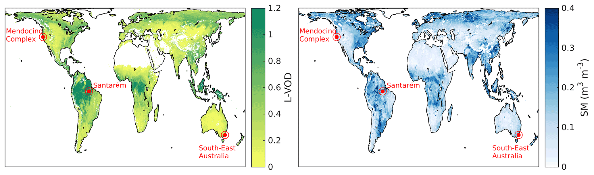
Figure 1 Global maps of SMOS L-VOD (left) and SM (right), with averages for 2011–2020. The red dots show the locations of the three areas of interest: the Mendocino Complex in California, Santarém in Amazonia, and the South Coast of New South Wales in Australia.

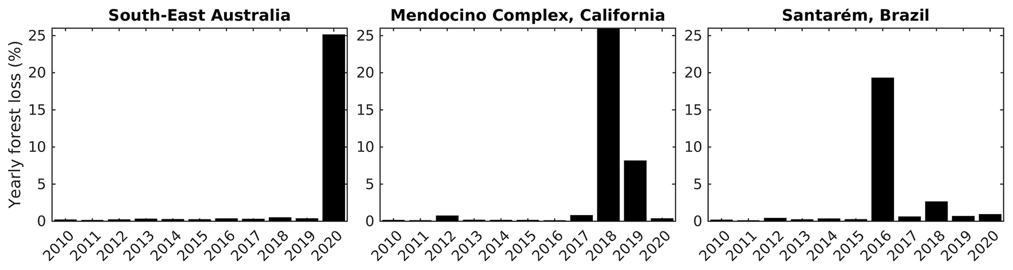
Figure 2 Yearly forest loss (%) attributed to the three burned areas under study, from the Hansen et al. (2013) “lossyear” product.

3.2.4 Anomaly time series computation

Anomaly time series of EVI; X-, C-, and L-VOD; P; SM; TWS; and T were plotted over the three studied sites. The anomaly (anom) time series of a variable x is the difference between the original time series and the mean climatology, which is the mean seasonal cycle of this variable. They are defined as

$$\begin{array}{}\text{(1)}& \mathrm{anom}\left(x\left(t\right)\right)=x\left(t\right)-\mathrm{climatology}\left(x\left(m\right)\right)\end{array}$$

and

$$\begin{array}{}\text{(2)}& \begin{array}{rl}\mathrm{climatology}\left(x\left(m\right)\right)& ={\displaystyle \frac{\mathrm{1}}{y_n}}{\sum }_{y=\mathrm{1}}^{y_n}x\left(m+\left(y-\mathrm{1}\right)\cdot \mathrm{12}\right),\\ \textcolor{red}{}m& =\mathrm{1}-\mathrm{12}\end{array}\end{array}$$

where t is the month number from January 2010 (6 to 132 in this study); m is the month of the year, between 1 and 12, with m= (t−1 mod 12) + 1; and y is the year number, from 1 to y_n, with y_n=11 here, as the climatology is computed for the period 2010–2020. Plotting the anomaly time series enables the removal of the natural seasonal cycle so as to observe only the variations due to specific events. The average pre-fire variable value was subtracted from the anomaly time series, only if at least 12 months of data were available before the fire event. It enables the observation of the anomalies with respect to the pre-disturbance value. The time series of the number of fires were plotted in absolute values.

3.3 Extension to the ecosystem scale

Fires were then studied at the ecosystem scale to assess the general factors and impacts of fire according to the specific features of each biome (Fig. 3). Five land cover classes were studied: grasslands and croplands (IGBP labels 10, 12, and 14), savannas and shrublands (IGBP labels 6, 7, 8, and 9), needleleaf forests (IGBP labels 1 and 3), sparse broadleaf forests (IGBP labels 2 and 4; AGB ≤ 150 Mg ha⁻¹), and dense broadleaf forests (IGBP labels 2 and 4; AGB > 150 Mg ha⁻¹). Only the latitude band 60^∘ S–60^∘ N was retained in order to be consistent with the precipitation dataset extent. Only the range July 2012–December 2020 was conserved here for all datasets so as to match with AMSR2 time period. For fire event selection, the time range was reduced from September 2013–October 2019 to avoid fire events occurring at the very beginning (or end respectively) of the period to be able to study possible pre- and post-fire anomalies. Only areas showing a unique and intense fire event over the 6-year period were considered to properly observe the factors and impacts of this event over a long time period without any other disturbance. This excluded dry areas with regular seasonal fires, such as the Sahel region. Two conditions were empirically defined as mandatory to select a fire event over a given pixel: (i) a minimum number of fires of 5 at the height of the fire and (ii) a maximum number of fires of 2.5 outside the period (±6 months) around the main fire event to ensure that the vegetation recovery is linked with the main fire event and is not affected by another significant one. Anomalies were computed with Eqs. (1) and (2), with a climatology over all dates excepted the year of the fire event, in order to remove these exceptional values. The anomaly time series were then shifted to collocate in time all fire events and averaged by ecosystem. To ensure the spatial representativeness of each ecosystem, the months with a number of available points lower than half the maximum number of points of the ecosystem were filtered out from the shifted time series.

Pre-fire climatic anomalies and post-fire vegetation anomalies were also aggregated at different timeframes and plotted, in order to compare their temporal behaviour in different ecosystems. The standard error of the mean of the measurements σ was also computed with Eq. (3):

$$\begin{array}{}\text{(3)}& \mathit{\sigma }\left(p\right)={\displaystyle \frac{\mathrm{SD}\left(p\right)}{\sqrt{n}}},\end{array}$$

where SD is the standard deviation of the population p and n is the number of samples.

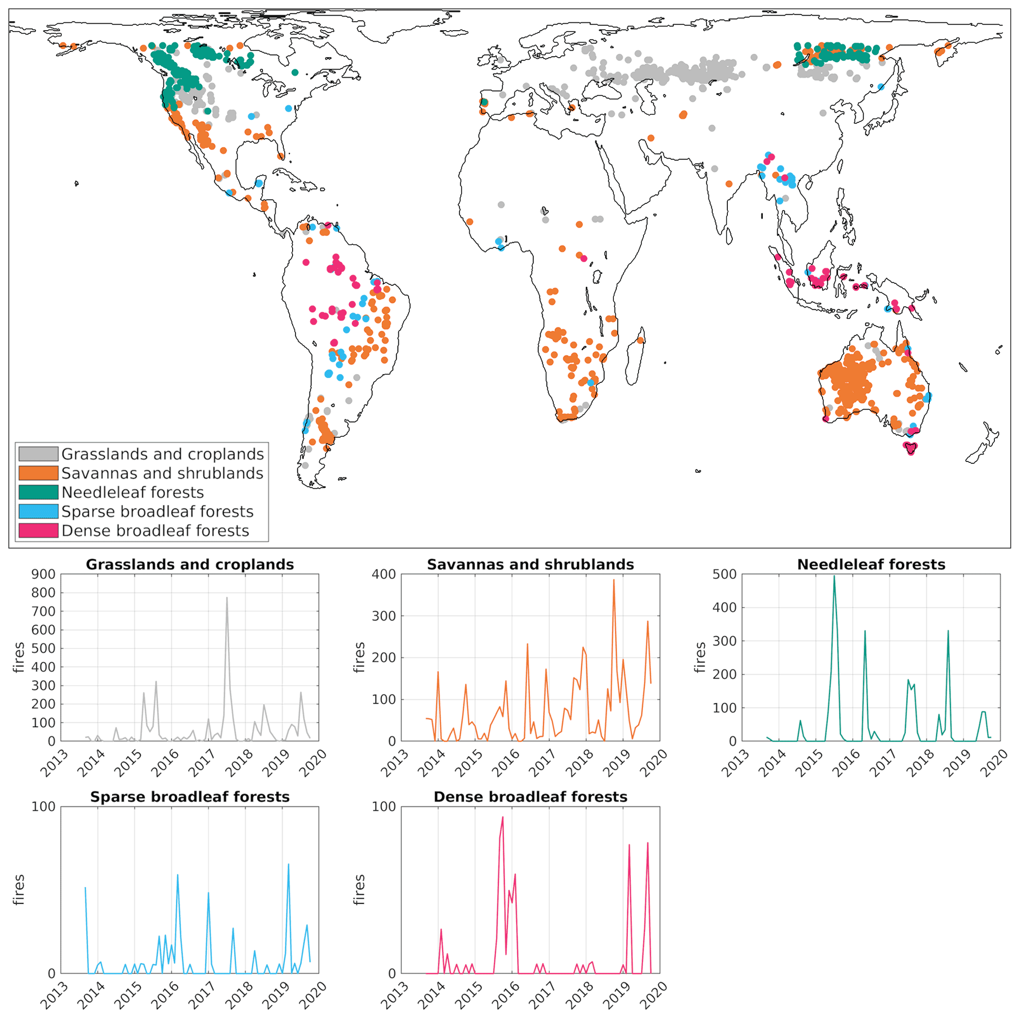
Figure 3 Location of the selected fires and histograms of the fire dates, for grasslands and croplands (IGBP labels 10, 12, and 14), savannas and shrublands (IGBP labels 6, 7, 8, and 9), needleleaf forests (IGBP labels 1 and 3), sparse broadleaf forests (IGBP labels 2 and 4; AGB ≤ 150 Mg ha⁻¹), and dense broadleaf forests (IGBP labels 2 and 4; AGB > 150 Mg ha⁻¹). Areas affected by water, snow, or strong topography were excluded (see Sect. 3.1).

4 Results

4.1 Case study: analysis of three major fires

In evergreen forests of the South Coast of New South Wales in Australia (Fig. 4a), fires reached a maximum in January 2020 (mean number of fires = 8). They are associated with high temperature and low precipitation (anom(T) = +3^∘ C, anom(P) = −80 mm). The drought started 3 years before fire (decrease in precipitation, SM, and TWS). All vegetation data exhibit the same pattern, which is (i) a constant and mild decrease since 2012, (ii) a strong decrease just before and during the fire event (∼ −0.15), and (iii) a rapid post-fire recovery (∼ 1 year). C-VOD is the most affected vegetation variable.

In California, no major pre-fire drought is visible in summer 2018 (Fig. 4b). The Mendocino Complex was the strongest of the three case studies, with 20 fires observed on average in August 2018. It provoked a decrease in all vegetation variables, particularly in L-VOD (anom(L-VOD) = −0.08) and in EVI (anom(EVI) = −0.10). Whereas C- and X-VOD regained their pre-fire values rapidly (∼ 1 year), EVI and L-VOD did not.

In the dense rainforest near Santarém (Brazilian Amazon), the number of detected fires in December 2015 is quite low (∼ 4.5) (Fig. 4c), but this value may be underestimated because of cloud coverage (Giglio et al., 2020). Vegetation variables are stable before the fire event, even if the L-VOD signal is quite noisy because only two SMOS pixels were considered here. Strong positive temperature anomalies (+3^∘ C), negative precipitation anomalies (−160 mm), and TWS anomalies (−60 cm) are visible during the fire and reach their extremum at the end of the fire period. Surprisingly, SM stayed stable during the fire. L-VOD was substantially impacted by the fire (anom(L-VOD) = −0.14), as well as EVI (anom(EVI) = −0.09). C- and X-VOD were barely affected (anom(C-VOD) = −0.04, anom(X-VOD) = −0.01). EVI recovered in ∼ 2–3 years, whereas L-VOD never recovered its pre-fire level.

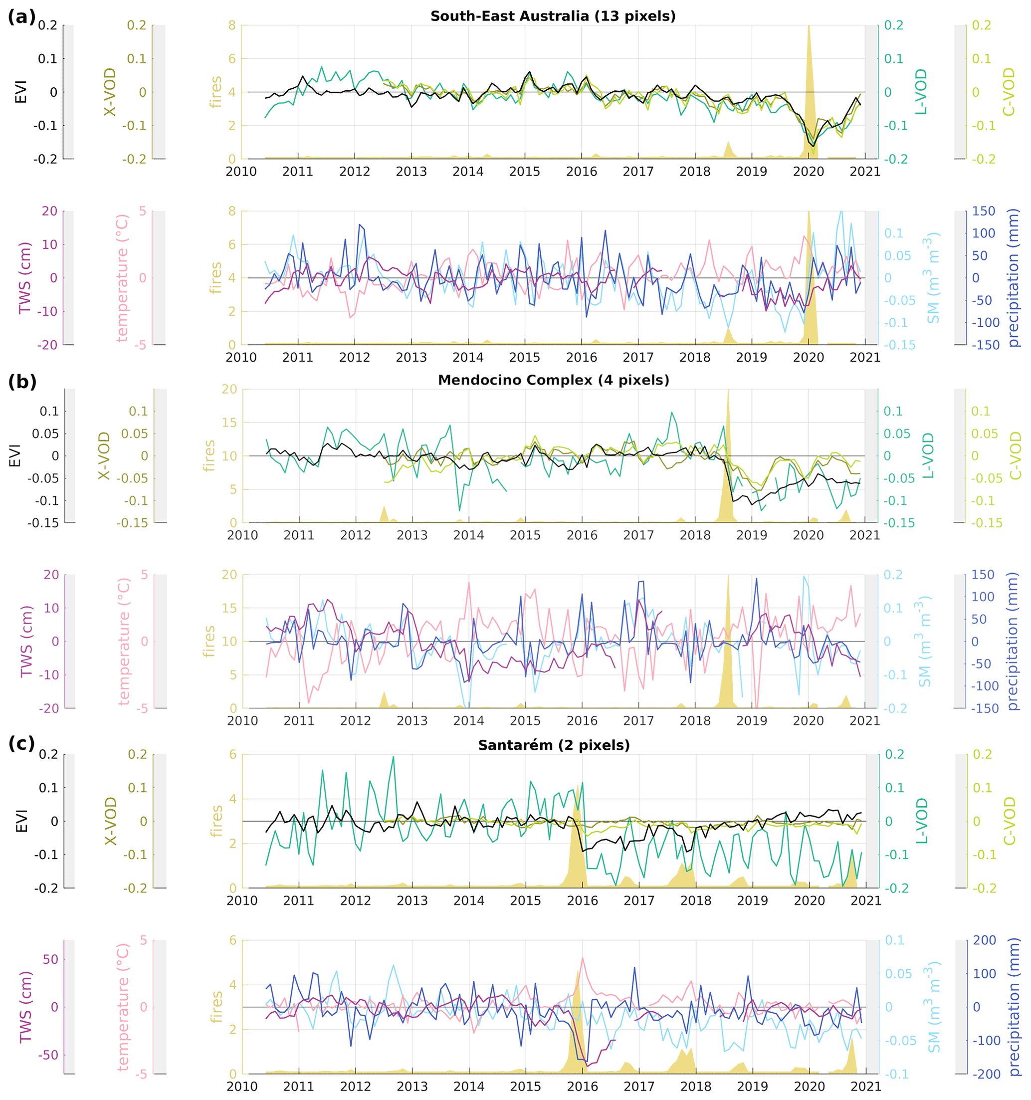
Figure 4 Time series of the number of fires and anomaly time series of EVI; X-, C-, and L-VOD; P; SM; TWS; and T for (a) south-east Australia (13 SMOS pixels); (b) the Mendocino Complex, California (4 SMOS pixels); and (c) Santarém (2 SMOS pixels).

4.2 Extension to the ecosystem scale

In this section, major fires from September 2013 to October 2019 were analysed at the ecosystem scale by shifting the anomaly time series of all variables on the fire date t_fire. The considered fires are well spread spatially and temporally over the 6-year period (Fig. 3). In grasslands and savannas (Fig. 5a and b), pre-fire anomalies of hydrologic variables are slightly positive, and temperature anomalies are negative during 2 years before fire. Concurrently, vegetation variables start to increase and reach a maximum a few months before the fire event (particularly C- and X-VOD). Anomalies of vegetation variables also show a light surplus over needleleaf forests just before the fire event (Fig. 5c). Over forests (Fig. 5c, d, e), a 1-year pre-fire drought is visible through the temperature increase and the decrease in precipitation, SM, and TWS. For all ecosystems, these drought conditions intensify just before and during fire and end a few months after fire. During fire, all vegetation variables abruptly decrease in all ecosystems, EVI being the most impacted one and also faster to recover. L-VOD is particularly long to recover over forests, especially dense broadleaf ones (more than 4 years, Fig. 5e). In needleleaf forests (Fig. 5c), VODs continue to decrease for 1 year. In low-vegetation ecosystems (Fig. 5a and b), C- and X-VOD never regain their immediate pre-fire values, which were particularly high.

Anomalies of climate variables were also averaged in space and in time, within timeframes of 6 months, from 24 to 1 month pre-fire, in order to observe their general trends (Fig. 6). The error bars were computed with Eq. (3). Precipitation anomalies (Fig. 6a) are negative from 6 months pre-fire for all classes and reach −15 mm per month on average before the fire event. The precipitation deficit is more intense in dense broadleaf forests, starting 2 years pre-fire and reaching −55 mm per month before the fire event. SM anomalies (Fig. 6b) are similar for the three forest classes. The SM deficit starts 18 months pre-fire and reaches −0.04 m³ m⁻³ before the fire event. Savannas and grasslands are affected later (6 months pre-fire) and to a lesser extent (∼ −0.01 m³ m⁻³), as previously observed in Fig. 5. TWS anomalies (Fig. 6c) are negative from 24 months pre-fire for needleleaf forests and from 6 months pre-fire for dense broadleaf forests. This ecosystem is again the most impacted one, with a minimum TWS anomaly of −7 cm before fire. Temperature anomalies (Fig. 6d) show significant negative anomalies in grasslands, savannas, and needleleaf forests from 2 to 1 year pre-fire. From 6 months pre-fire, temperature anomalies show a surplus in nearly all ecosystems and reach +1.1^∘ C in needleleaf forests and +0.7^∘ C in dense broadleaf forests before the fire event. In summary, pre-fire drought is mainly observed in forests, with particularly low hydrological values in dense forests (rainforests) and particularly high temperatures in needleleaf forests (boreal ecosystems). Savannas and grasslands barely suffer from pre-fire drought; temperatures are even mild 1 year pre-fire.

Vegetation variable anomalies were averaged within timeframes of 6 months, from 1 to 36 months post-fire, in order to observe the global impacts and recovery time (Fig. 7). We considered that a variable has totally recovered when its anomaly is between −0.005 and +0.005. Immediately after fire, EVI is the most impacted variable, with average anomalies of −0.026 over grasslands, −0.022 over savannas, −0.033 over needleleaf forests, −0.051 over sparse broadleaf forests, and −0.048 over dense broadleaf forests (Fig. 7a). EVI recovers rapidly, in about 25 to 30 months. X-VOD is less affected over forests (−0.015) than over low vegetation (−0.025) (Fig. 7b). X-VOD gets back to normal within 3 years, savannas and shrublands taking the longest to recover. C-VOD recovers slower than X-VOD, in particular over forests (Fig. 7c). L-VOD is mainly affected over dense broadleaf forests (Fig. 7d). Negative anomalies decrease up to −0.05 6 months post-fire, then slowly increase. L-VOD is less affected than C-VOD elsewhere. It also shows a delayed impact over needleleaf forests, as for C- and X-VOD.

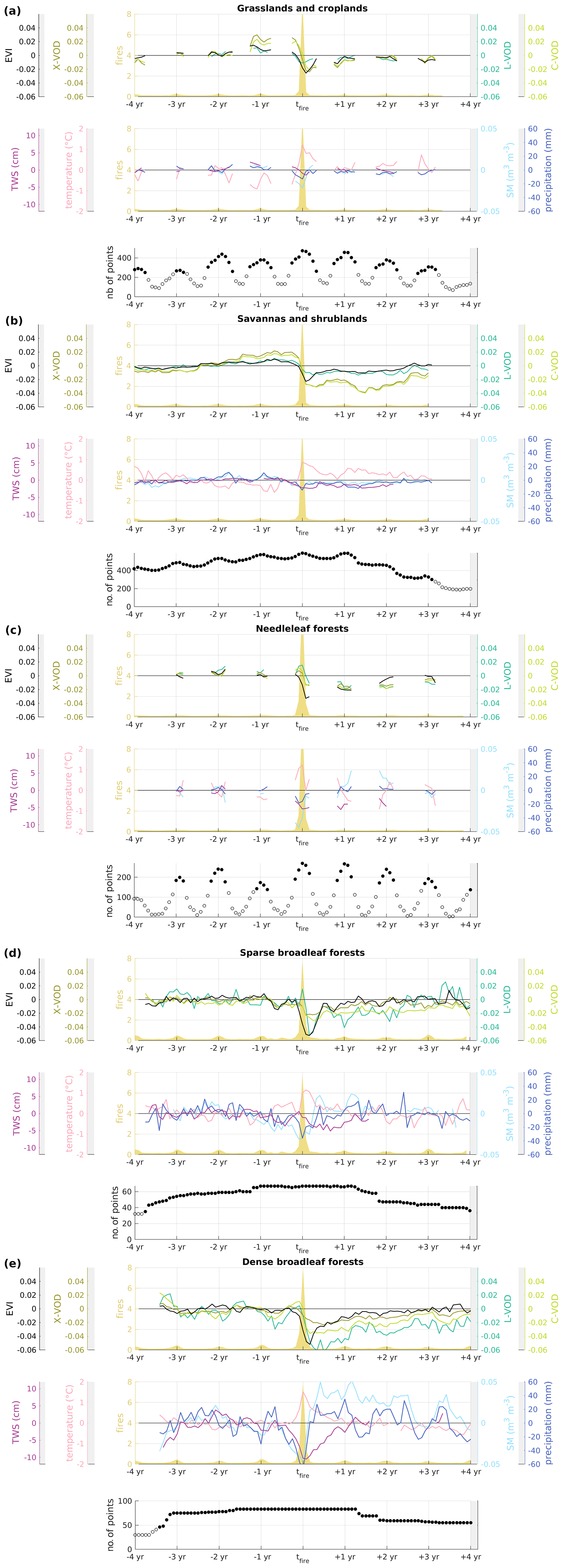
Figure 5 Time series of the number of fires and anomaly time series of EVI; X-, C-, and L-VOD; P; SM; TWS; and T, shifted on the fire date, for the following biomes: (a) grasslands and croplands, (b) savannas and shrublands, (c) needleleaf forest, (d) sparse broadleaf forest, and (e) dense broadleaf forest. Missing values appear when the number of available points is lower than half the maximum number of points of the biome (empty circles in the lower panel). This is mostly due to snow filtering. Data are kept otherwise (black filled dots).

5 Discussion

5.1 Case study: analysis of three major fires

In south-east Australia, a strong pre-fire drought is visible not only in the climate variables but also in the mild decrease in vegetation variables (Fig. 4a), linked with VWC deficit. Ehsani et al. (2020) stated that the air temperature from December 2019 to February 2020 was about 1^∘ C higher than usual, which increased evapotranspiration, while the lack of precipitation prevented the soil from satisfying the moisture demand and led to a significant vegetation drying (fuel) that facilitated the propagation of fires. After the fire event, L-VOD regained its pre-fire values within a year, meaning that the woody biomass was not entirely destroyed. Indeed, these eucalyptus forests are known to be somewhat fire resistant (Wilkinson and Jennings, 1993; Caccamo et al., 2015). They can regenerate branches and leaves by resprouting from heat-resistant buds (Burrows, 2002). The rapid recovery of vegetation data can also be explained by the recovery of VWC, linked with the post-fire increase in precipitation and SM (Konings et al., 2021). Indeed, in 2020, SM values exceeded those of the previous decade (anom(SM) = +0.15 m³ m⁻³), corresponding to the end of the severe drought affecting south-east Australia associated with the 2020–2021 La Niña event (BoM, 2021). The increase in SM and precipitation may also have expedited the extinction of fires (Ehsani et al., 2020).

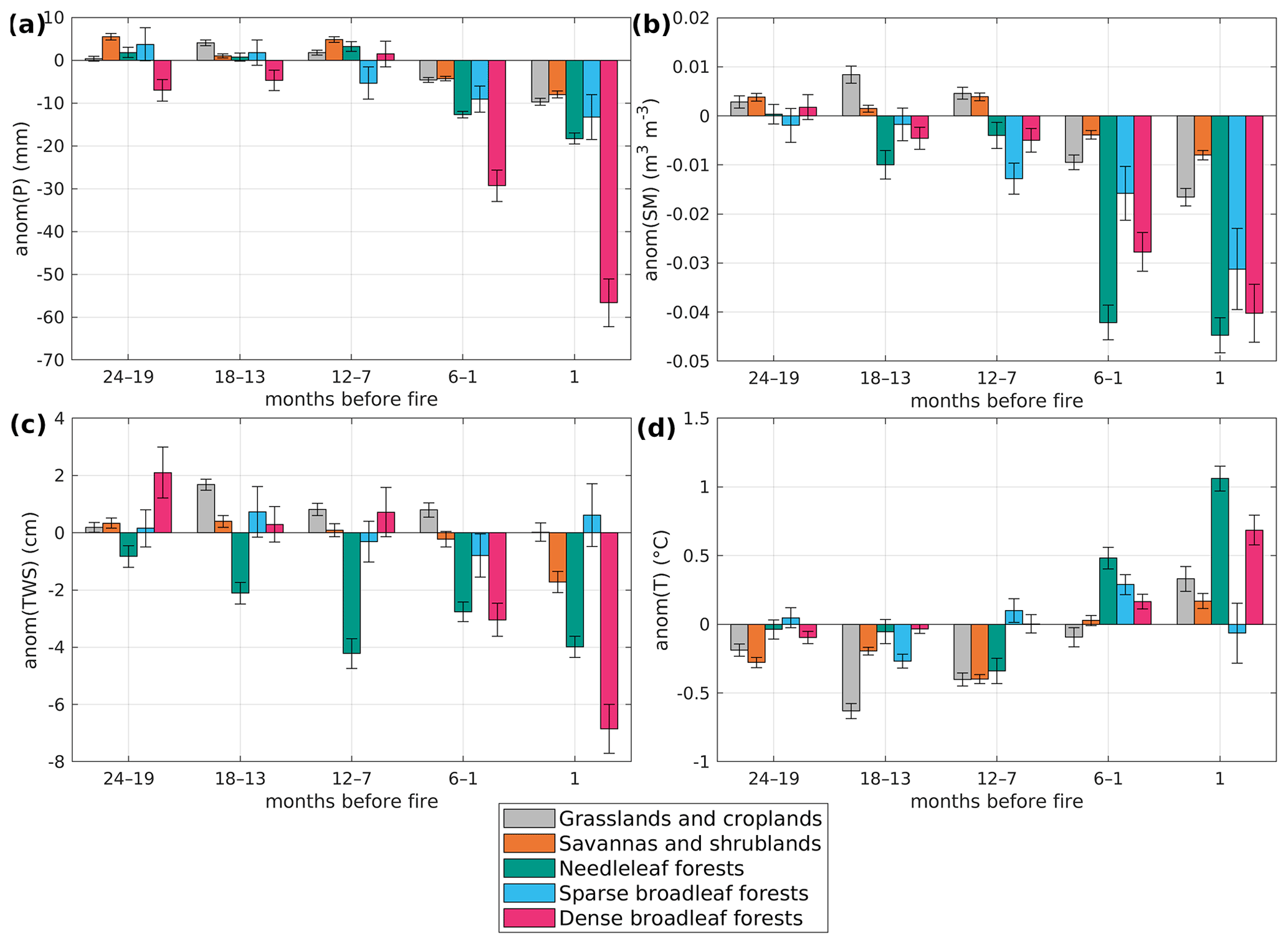
Figure 6 Anomalies of (a) precipitation, (b) SM, (c) TWS, and (d) temperature, for each ecosystem, at several pre-fire timescales. The error bars were computed with Eq. (3).

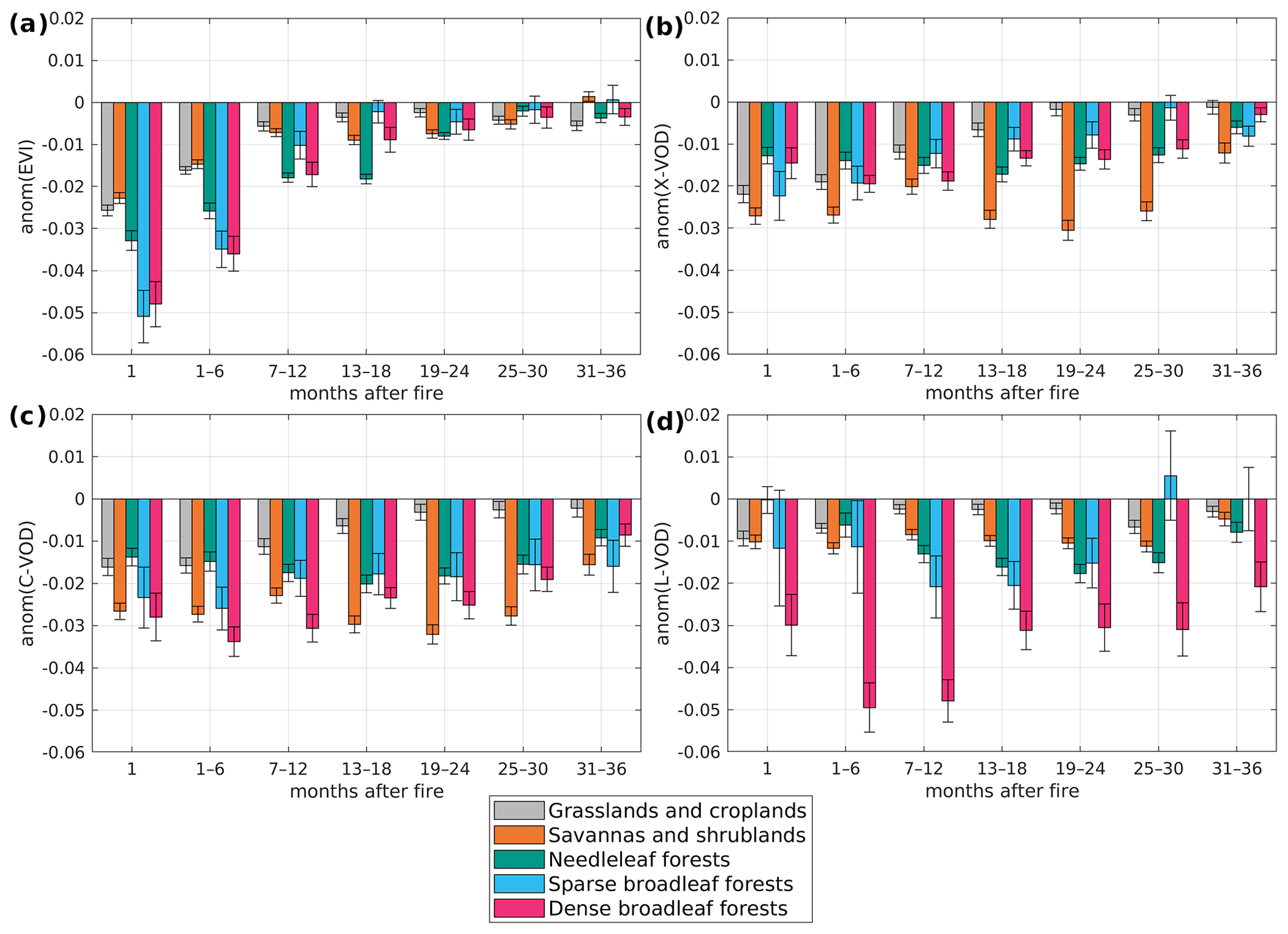
Figure 7 Anomalies of (a) EVI, (b) X-VOD, (c) C-VOD, and (d) L-VOD, for each ecosystem, at several post-fire timescales. The error bars were computed with Eq. (3).

For California, the study by Brown et al. (2020) provides a comprehensive analysis of the climate and fuel conditions leading to the 2018 Mendocino Complex and reports several events that are also noticeable in our analysis. Among these, positive rainfall and SM anomalies in winter 2016/17 are depicted in Fig. 4b, which led to the second consecutive spring with above-average accumulation of fine fuel (grasses). Positive temperature anomalies in winter 2017/18 are also visible, when a lack of storm enabled the survival of grasses. In April 2018, precipitation and warm temperatures led to above-normal spring brush and grass growth. No major drought is visible in summer 2018, but low rainfall and warm temperatures led to a rapid drying of fuels and induced a poor overnight humidity recovery. All these similarities with the findings by Brown et al. (2020) support our observations. The dramatic fire impacted EVI and L-VOD in the long term. Eucalyptus, pine trees, and chaparral were burned. Even if this type of vegetation is fire-adapted, the strength of the fire seemed to have destroyed most of it (34 % vegetation loss, Hansen et al., 2013). Increased forest fire activity in recent decades in California has likely been enabled by the legacy of fire suppression, human settlement, and anthropogenic climate change (Abatzoglou and Williams, 2016). Stephens et al. (2018) stated that the massive current tree mortality in California will undoubtedly provoke severe “mass fires” in the coming decades, driven by the amount of dry and combustible wood.

In the Santarém region (Amazon), the winter 2015 wildfire was attributed to high temperature and low precipitation linked with El Niño event (Berenguer et al., 2018), which clearly emerges from Fig. 4c. These extreme drought conditions worsened during and at the end of the fire and may explain its strength. Several factors can explain this observation. First, MODIS may not detect all fires in January 2016 in this area because of (i) the cloud coverage (Roy et al., 2008) and (ii) the dense vegetation cover hiding understorey fires (Withey et al., 2018). This would be in line with the 2016 Hansen et al. (2013) tree cover loss detection (Fig. 2). Secondly, drought may sometimes keep increasing after fire extinguishment because the removal of the vegetation cover and the deterioration of the soil contributes to maintaining a hot and dry climate (Auld and Bradstock, 1996; Veraverbeke et al., 2010). This phenomenon is also visible in the savanna and in the sparse broadleaf biome (Fig. 5b and d). Contrary to TWS and precipitation, SM stayed stable during the fire, maybe because of the reduced accuracy of SM measurements under very dense forest. The 3-year recovery time of EVI after the severe fire indicates a moderate regrowth of leaves and grasses. In contrast, L-VOD never regained its pre-fire values, meaning that trunks were impacted in the long term.

5.2 Extension to the ecosystem scale

Grasslands, croplands, shrublands, and savannas do not show signs of pre-fire drought (Figs. 5a, b and 6). Indeed, in these dry ecosystems, the standard summer conditions are often prone to wildfire ignitions (Chaparro et al., 2016). A substantial increase in vegetation variables, C- and X-VOD in particular, occurs 1 to 2 years before fire, which implies an increase in vegetation density, e.g. available fuel. This is consistent with the fact that the C and X bands are more sensitive to dry low shrubland vegetation (Jackson et al., 1982; de Jeu et al., 2008). Immediately before fire, both VOD and SM values drop down, suggesting a decrease in VWC, especially over grasslands (Fig. 5a). The increase in vegetation material combined with the decrease in VWC may contribute to triggering large wildfires (Forkel et al., 2017; Kuhn-Régnier et al., 2021). Indeed, the fire risk in savannas is highest for dry vegetation with enough fuel to enable drastic burning (Mbow et al., 2004). This vegetation growth might be enabled by negative pre-fire temperature anomalies and a light positive anomaly in pre-fire hydrological variables (Fig. 6). Vegetation variables are less impacted by fires (Fig. 7), which are rapid and burn through the grass layer, resulting in less destruction than in forests (Menaut et al., 1990; Gignoux et al., 1997). L-VOD in particular is slightly impacted because the burned vegetation is mainly leaf biomass. EVI quickly recovers after fire, probably because fire burns most of the AGB of grass species but spares their large underground root systems, resulting in a rapid establishment of new shoots (Hochberg et al., 1994). The exceptionally high pre-fire vegetation variable values are never regained.

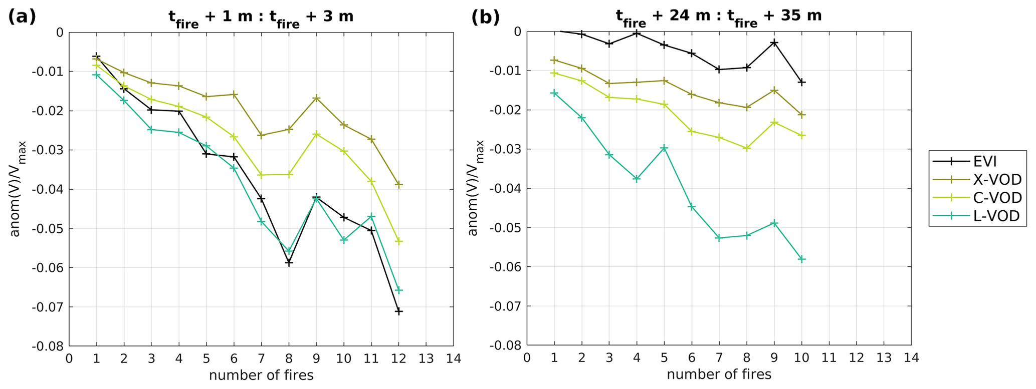
Figure 8 Anomalies of vegetation variables (V) averaged (a) from 1 to 3 months post-fire and (b) from 24 to 35 months post-fire, with respect to the number of fires by pixel (MODIS), for dense broadleaf forests only. The anomalies were normalized with the 99th quantile of each variable V_max (EVI_max=0.60, X-VOD_max=1.03, C-VOD_max=1.20, and L-VOD_max=1.20).

In needleleaf forest anomaly time series (Fig. 5c), the numerous missing values correspond to the filtering of snow in winter. These wildfires are located in the Northern Hemisphere temperate and boreal forests and mostly occur in late spring and summer (Fig. 3). De Groot et al. (2013) explained that most fires in Canada occur during summer, due to lightning strikes, whereas most fires in Russia occur during spring and are human-caused. We found a strong pre-fire drought in this ecosystem (low SM and high temperature 1 year pre-fire, Fig. 6), which is well documented for previous fire episodes (Weber and Stocks, 1998). Our results are in line with those of Forkel et al. (2012), who found that previous-summer SM was a good predictor for burned area in Siberian larch forests. Indeed, negative summer anomalies led to low frozen water the following winter and to less water being released during the following spring–summer season, which in turn eased the outbreak of large wildfires. VODs also showed a light surplus before fire, possibly linked with litter thickening (e.g. dead needles, cured grass, leaf litter), which also facilitates fire propagation (de Groot et al., 2013). We found a delayed impact of fire on vegetation variables, as well as a longer recovery time than in other ecosystems, of about 3–4 years (Figs. 5c and 7). This duration is slightly less than what was found in other studies (5 years in Canada, Goetz et al., 2006; 5 to 8 years in North America, Jin et al., 2012), but our findings still confirm previous results from Yang et al. (2017), who showed with NDVI analyses over North America that the fire effect on needleleaf trees was stronger and longer than on other vegetation types. Fires in North America are predominantly stand-replacing and high-intensity crown fires (Stocks et al., 2004; Jin et al., 2012), whereas fires in Eurasia are generally lower-intensity surface fires and less destructive for the vegetation (de Groot et al., 2013). These different fire regimes are influenced by tree species (Rogers et al., 2015). Time series were plotted separately over each continent (Fig. S1). L-VOD and EVI recover more slowly in North America than in Eurasia (∼ 4 vs. ∼ 2 years for L-VOD, ∼ 3 vs. ∼ 2 years for EVI), confirming these different boreal fire regimes. Moreover, we found that L-VOD is moderately impacted during fire, which can be attributed to the dominant destruction of needles and branches by boreal fires (Alexander and Cruz, 2011).

Sparse broadleaf forests (AGB ≤ 150 Mg ha⁻¹) subject to wildfires are mostly located in subtropical and temperate areas of the Americas, West Africa, Australia, and South-East Asia (Fig. 3). A drying trend is visible 1 year pre-fire (Figs. 5d and 6). The link between drought and wildfires was previously observed by de Marzo et al. (2021) in the Argentine Gran Chaco, by Cheng et al. (2013) in the Mexican Yucatán forest, and by Vadrevu et al. (2019) in South-East Asian forests, with a prominent influence of precipitation variations over temperature variations. L-VOD and EVI are particularly impacted by fire, but they recover quickly (1 year for EVI, 2.5 years for L-VOD). Yang et al. (2017) also found a rapid recovery time over North American broadleaf trees due to their fire-adaptive resprouting regeneration mode. The same observations were made in the fire-prone Argentine Chaco forest by Torres et al. (2014).

Dense broadleaf forests are mostly located in the tropics (Fig. 3). We can notice a few fires in the densest rainforests (Congo basin, central Amazon) because (i) they are usually too humid to burn (Cochrane, 2003; Forkel et al., 2017), (ii) MODIS active fire detections are underestimated under thick cloud coverage or for understorey fires (Giglio et al., 2020), and (iii) seasonally flooded areas were excluded in order to use only robust VOD estimations (Bousquet et al., 2021). A consistent drought is visible 8 months before fire events (Fig. 5e), with high negative SM, TWS, and precipitation anomalies (Fig. 6). Chen et al. (2013) also found TWS deficits before severe fire seasons across the southern Amazon. Indeed, rainfall shortage generates high water deficits (i.e. high negative TWS and SM anomalies), which cause tree mortality and leaf shedding (visible in pre-fire EVI decrease) and thus increase fuel availability (Aragão et al., 2018). Nevertheless, no pre-fire VOD decrease is observed here, showing that tree species of dense forests can maintain their VWC. Drought-related fires were suggested to prevail over deforestation fires in the Amazon and are predicted to increase in the near future (Aragão et al., 2018). The opening of forest canopies also boosts incident radiation levels which leads to temperature rise (Ray et al., 2005). The combination of fuel increase in a drier and hotter environment converts forests into fire-prone ecosystems (Aragão et al., 2018). We also found that dense broadleaf forests were the ecosystem most impacted by fire (Fig. 7) because the absolute pre-fire values of vegetation variables are particularly high and because it is not a fire-adapted ecosystem (Cochrane, 2003). L-VOD in particular decreases strongly and recovers very slowly (Fig. 7d), as previously observed over the Santarém fire (Fig. 4c). The strong post-fire decrease in L-VOD is due not only to biomass destruction but also to water stress in the remaining vegetation (Konings et al., 2021). This finding confirms the significant and damaging impact of fires in the dense broadleaf ecosystem previously observed by Silva et al. (2018) and de Faria et al. (2021). L-VOD was previously proven to be more sensitive to high AGB values than C- and X-VOD (Rodriguez-Fernandez et al., 2018). Here, we suggest that L-VOD depicts the fire impact on high-AGB areas better than the other vegetation variables.

For all biomes, EVI is the most rapid index to recover, because leaves rapidly resprout. EVI and X-VOD seem better adapted for grassland fire monitoring; C-VOD is better for savanna fire monitoring; and L-VOD is better for forest fire monitoring.

5.3 The potential of L-VOD for vegetation recovery monitoring over dense forests

Normalized anomalies of vegetation variables were also plotted with respect to the number of fires in the dense broadleaf ecosystem, immediately after fire (1–3 months post-fire, Fig. 8a) and over a longer period (1–2 years post-fire, Fig. 8b). A quasi-linear relationship is visible between all vegetation estimates and the number of fires. As previously observed in Sect. 4.2, EVI and L-VOD are the most impacted variables immediately after fire (Fig. 8a), while L-VOD is still significantly affected 1 to 2 years after fire (up to −0.06, Fig. 8b). L-VOD then shows a clear response to fire events over high-AGB areas, not only immediately but also in the long term and proportionally to the number of fires within a SMOS pixel. Thanks to its sensitivity to coarse woody elements and to its deep penetration through the vegetation layer, L-VOD is better correlated with high AGB than other vegetation variables (Rodriguez-Fernandez et al., 2018) and could be used for post-fire recovery monitoring over dense forests. One must keep in mind that not only the biomass density (AGB) but also its hydrological status (VWC) are depicted in the VOD.

6 Conclusions

In this paper, we analysed the pre-fire behaviour of four satellite-based fire likelihood factors, including SMOS SM. In forests, which generally maintain a steady humidity, we found that fires are linked with intense and prolonged drought. Pre-fire temperature anomalies are particularly high in boreal needleleaf forests. In savannas and grasslands, in agreement with previous studies (Mbow et al., 2004), we found evidence of an increase in available fuel prior to fire events, enabled by humid and cold conditions a few years before. We also found that vegetation variables recover rapidly in these ecosystems, as wildfires are often rapid and mildly destructive for trees. In contrast, over forests, fires can damage the vegetation in the long term. Zhang et al. (2021) demonstrated the potential of C-band vegetation optical depth to detect the vegetation change patterns caused by fire in the southern Amazon. Our study confirms these findings and extends it to the ecosystem scale and to two extra wavelengths. Dense broadleaf forest fires particularly impact the L-band emission, which represents coarse woody elements (trunks and stems), whereas sparse vegetation fires affect the C and X bands more, which are more sensitive to small branches and leaves. For all biomes, the visible-infrared index (EVI) drops down after fire but recovers quickly, as it represents only herbage and canopy foliage. The long-term impact on L-VOD in dense broadleaf forests shows that fires in this ecosystem are severely destructive for trunks, while smaller woody elements and leaves resprout faster. Thus, L-VOD seems to be the best-adapted vegetation variable for the monitoring of dense vegetation recovery after large fires.

The increasing number of wildfires threatens the stability of several ecosystems. It is then particularly important to monitor the vegetation health, and the L band proved to be complementary to existing measurements, especially over dense forests.