The sensitivity of pCO₂ reconstructions to sampling scales across a Southern Ocean sub-domain: a semi-idealized ocean sampling simulation approach

The Southern Ocean is a complex system yet is sparsely sampled in both space and time. These factors raise questions about the confidence in present sampling strategies and associated machine learning (ML) reconstructions. Previous studies have not yielded a clear understanding of the origin of uncertainties and biases for the reconstructions of the partial pressure of carbon dioxide (pCO₂) at the surface ocean ($p{\mathrm{CO}}_{\mathrm{2}}^{\mathrm{ocean}}$). We examine these questions through a series of semi-idealized observing system simulation experiments (OSSEs) using a high-resolution (± 10 km) coupled physical and biogeochemical model (NEMO-PISCES, Nucleus for European Modelling of the Ocean, Pelagic Interactions Scheme for Carbon and Ecosystem Studies). Here we choose 1 year of the model sub-domain of 10^∘ of latitude (40–50^∘ S) by 20^∘ of longitude (10^∘ W–10^∘ E). This domain is crossed by the sub-Antarctic front and thus includes both the sub-Antarctic zone and the polar frontal zone in the south-east Atlantic Ocean, which are the two most sampled sub-regions of the Southern Ocean. We show that while this sub-domain is small relative to the Southern Ocean scales, it is representative of the scales of variability we aim to examine. The OSSEs simulated the observational scales of $p{\mathrm{CO}}_{\mathrm{2}}^{\mathrm{ocean}}$ in ways that are comparable to existing ocean CO₂ observing platforms (ships, Wave Gliders, carbon floats, Saildrones) in terms of their temporal sampling scales and not necessarily their spatial ones. The pCO₂ reconstructions were carried out using a two-member ensemble approach that consisted of two machine learning (ML) methods, (1) the feed-forward neural network and (2) the gradient boosting machines. The baseline data were from the ship-based simulations mimicking ship-based observations from the Surface Ocean CO₂ Atlas (SOCAT). For each of the sampling-scale scenarios, we applied the two-member ensemble method to reconstruct the full sub-domain $p{\mathrm{CO}}_{\mathrm{2}}^{\mathrm{ocean}}$. The reconstruction skill was then assessed through a statistical comparison of reconstructed $p{\mathrm{CO}}_{\mathrm{2}}^{\mathrm{ocean}}$ and the model domain mean. The analysis shows that uncertainties and biases for $p{\mathrm{CO}}_{\mathrm{2}}^{\mathrm{ocean}}$ reconstructions are very sensitive to both the spatial and the temporal scales of pCO₂ sampling in the model domain. The four key findings from our investigation are as follows: (1) improving ML-based pCO₂ reconstructions in the Southern Ocean requires simultaneous high-resolution observations (<3 d) of the seasonal cycle of the meridional gradients of $p{\mathrm{CO}}_{\mathrm{2}}^{\mathrm{ocean}}$; (2) Saildrones stand out as the optimal platforms to simultaneously address these requirements; (3) Wave Gliders with hourly/daily resolution in pseudo-mooring mode improve on carbon floats (10 d period), which suggests that sampling aliases from the 10 d sampling period might have a greater negative impact on their uncertainties, biases, and reconstruction means; and (4) the present seasonal sampling biases (towards summer) in SOCAT data in the Southern Ocean may be behind a significant winter bias in the reconstructed seasonal cycle of $p{\mathrm{CO}}_{\mathrm{2}}^{\mathrm{ocean}}$.

1 Introduction

The Southern Ocean (SO) remains the world's largest modulator for the ocean uptake of anthropogenic CO₂ (Sabine et al., 2004; Frölicher et al., 2015; Friedlingstein et al., 2020). Therefore, reducing uncertainties and biases in CO₂ budget estimates in the region is important to better assess and understand the Southern Ocean's influence on regional and global climate (Majkut et al., 2014; Gruber et al., 2019; Hauck et al., 2020). For instance, since the early 2000s, the SO carbon sink has undergone a reinvigoration characterized by a substantial strengthening as reported by Landschützer et al. (2015), following a decade (the 1990s) of weakening trends (Canadell et al., 2021; Le Quéré et al., 2007). Based on these findings, many studies have been conducted recently to investigate what drives these inter-annual and decadal changes in the SO carbon sink and assess the uncertainties in the estimates (Bushinsky et al., 2019; DeVries et al., 2017; Fay et al., 2018; Gregor et al., 2018, 2019; Landschützer et al., 2016; McKinley et al., 2020). However, there have not been many studies looking into the role of intra-seasonal and seasonal modes of variability in the uncertainties and biases reported in empirical CO₂ mapping approaches (Landschützer et al., 2016; Gregor et al., 2019). In this region, surface ocean CO₂ observations underlying CO₂ reconstructions are very sparse, especially during the stormy autumn and winter seasons, requiring a substantial number of extrapolations to map and subsequently fill the gaps due to data sparseness (Gregor et al., 2017, 2019; Landschützer et al., 2014).

Many empirical approaches such as statistical interpolations and regression methods (Iida et al., 2015; Jones et al., 2015; Rödenbeck et al., 2014) had been gaining attention as alternative methods to ocean biogeochemical models (Lenton et al., 2013) until recently when machine learning (ML) approaches have been used increasingly as an alternative (Denvil-Sommer et al., 2019; Gregor et al., 2017, 2019; Landschützer et al., 2013, 2014, 2016). These novel mapping methods all seek to fill the spatial and temporal sampling gaps from existing ship-based surface ocean CO₂ observations by extrapolating the CO₂ partial pressure (pCO₂) at the surface ocean ($p{\mathrm{CO}}_{\mathrm{2}}^{\mathrm{ocean}}$) using prognostic proxy variables (such as satellite-observed and re-analysis-based sea surface temperature, sea surface salinity, mixed-layer depth, chlorophyll a). The feasibility of these extrapolations is justified through the non-linear relationships between the surface ocean pCO₂ and the above-mentioned prognostic variables that may drive changes in the surface ocean pCO₂ (Takahashi et al., 1993).

Historically, surface ocean CO₂ observations were primarily from voluntary observing ships including research and commercial vessels (Bakker et al., 2012; Pfeil et al., 2013). These pCO₂ observations are thus intrinsically biased by the sampling limitations in space and time for the past several decades covering only ∼ 2 % of all the monthly 1^∘ observational grid points (Bakker et al., 2016; Sabine et al., 2013). Mainly due to its remoteness and harsh weather especially during stormy autumn and winter, it has been increasingly shown that the SO is the ocean region that contributes the most to these uncertainties in the contemporary estimates of the mean annual CO₂ uptake (Bushinsky et al., 2019; Gloege et al., 2021; Gregor et al., 2019; Ritter et al., 2017). For instance, sparse observations in largely inaccessible SO areas, particularly during the stormy wintertime, have been the biggest barrier to constraining the seasonal cycle of regional and global contemporary ocean–atmosphere CO₂ exchange (Bakker et al., 2016; Monteiro et al., 2015; Ritter et al., 2017; Rödenbeck et al., 2015).

Complementary to the increasing effort in the shipboard CO₂ observations through the Surface Ocean CO₂ Atlas (SOCAT) initiative, the ongoing development of autonomous ocean observing systems, such as biogeochemical floats and Wave Gliders, has started to significantly improve the spatial and temporal coverage of CO₂ samples in the SO in recent years (Bakker et al., 2016; Bushinsky et al., 2019; Gray et al., 2018; Monteiro et al., 2015). Over the last decade, the advent of a range of new autonomous ocean observing platforms has opened doors towards closing the seasonal and intra-seasonal sampling biases created by the high cost of ship operations in the Southern Ocean outside the summer window (Bushinsky et al., 2019; Gray et al., 2018; Majkut et al., 2014; Monteiro et al., 2015; Sutton et al., 2021; Williams et al., 2017).

Thus resolving the mean seasonal cycle and intra-seasonal mode of variability through in situ observations not only is a challenging exercise but also has followed several avenues from extrapolating findings from the Drake Passage Time-series (DPT) like in Fay et al. (2018) to utilizing measurements from extended deployments of autonomous ocean observing platforms such as Wave Gliders (Monteiro et al., 2015; Nicholson et al., 2022), biogeochemical Argo floats (Bushinsky et al., 2019; Gray et al., 2018; Williams et al., 2017), and more recently Saildrones (Sutton et al., 2021). These advances have allowed the density of the Southern Ocean surface CO₂ observing networks to increase, particularly in the sub-Antarctic zone (SAZ) and polar frontal zone (PFZ), which to date are the most observed sub-regions of the SO. Consequently, the problem of general sparseness in observations and particularly of the sampling biases (Gloege et al., 2021; Monteiro et al., 2015) has been partially addressed but not resolved by the ocean CO₂ in situ observations community (Bushinsky et al., 2019; Sutton et al., 2021). For example, under-sampling in winter by ships has been addressed by the 10 d resolution SOCCOM (Southern Ocean Carbon and Climate Observations and Modeling) profiling floats and/or pseudo-Lagrangian platforms that are carried zonally by water currents (Bushinsky et al., 2019; Gray et al., 2018; Majkut et al., 2014; Monteiro et al., 2015; Sutton et al., 2021; Williams et al., 2017). Williams et al. (2017) and then Gray et al. (2018) reported on persistent differences found with previous pCO₂ estimates when the ship-based sampling is sparse, especially during winter, though a recent study seems to disagree on the persistence of these differences (Bushinsky et al., 2019). Therefore, an increase in winter sampling would yield a reduction in the uncertainty levels of surface ocean pCO₂ estimates (Bushinsky et al., 2019; Gregor et al., 2019). Notwithstanding these new platforms, sparse and scale-sensitive observations in the Southern Ocean continue to be a barrier to constraining the seasonal cycle and inter-annual variability in surface ocean pCO₂ (Monteiro et al., 2015; Rödenbeck et al., 2015; Sutton et al., 2021).

However, we appear to have reached a limit in terms of improving the uncertainties and biases underlying pCO₂ reconstructions as reported by Gregor et al. (2019). According to the authors, the performance measures in existing empirical methods converge, which led the authors to the rhetorical question, “have we hit the wall?” In practice, high-quality in situ CO₂ observations like those annually collected and compiled within the SOCAT database (primarily from ships) are fundamental to novel machine learning (ML) methods (Bakker et al., 2016; Sabine et al., 2013), despite the reconstructions being limited by spatial and temporal observational gaps and biased sampling (Gregor et al., 2019). As a result, our understanding of the derived impacts of the Southern Ocean dynamics, particularly seasonal and intra-seasonal modes of variability, has remained comparatively poor (Gruber et al., 2019), which may have also contributed to errors in the pCO₂ estimates. At a global scale, Gloege et al. (2021) coupled an observing system simulation experiment (OSSE) with Earth system models to quantify errors in observation-based reconstructions of air–sea CO₂ exchange by using one of the current gap-filling techniques, the self-organizing map feed-forward neural network (SOM-FFN) by Landschützer et al. (2016). The authors found that errors were regionally high in the Southern Hemisphere, particularly in the SO, for which insufficient sampling led to a 31 % (15 %–58 %) overestimation of decadal variability, but they did not discuss the perspective of uncertainties and biases due to the intra-seasonal mode of variability.

This study aims to investigate the sensitivity of the pCO₂ reconstructions to the spatio-temporal sampling scales of surface ocean CO₂ observing systems under the assumption that intra-seasonal modes of variability are critical to addressing reconstruction uncertainties and biases. To do that, we used a 1-year high-resolution (± 10 km) coupled physical and biogeochemical forced ocean model for a Southern Ocean sub-region that represents the scales of variability that we aim to resolve. Then, we conducted a series of semi-idealized OSSEs based on existing CO₂ observing platforms (ships, Wave Gliders, carbon floats, Saildrones) and coupled these with an ensemble of two state-of-the-art machine learning techniques (ML2). A rigorous assessment of the experiment scenarios is conducted through testing and understanding of the ML2 capabilities. We explore the question set by Gregor et al. (2019) about the prediction uncertainties and biases in contemporary pCO₂ reconstructions being now constrained by the sampling scales achievable by the existing ocean observing platforms. We make proposals towards significantly advancing machine learning reconstructions “beyond the wall”. The goal is to find out how the ocean carbon cycle community can better supplement ship-based observations, essential to pCO₂ reconstructions, with autonomous platform samples in order to reduce the uncertainties and biases in machine-learning-based mapping approaches.

2 Materials and methods

2.1 Data source

The data used in this study are from a year-long period of high-resolution (± 10 km) ocean model simulations. This ocean model is a regional configuration (BIOPERIANT12-CNCRUN05A-S) of the state-of-the-art ocean modelling framework NEMO (Nucleus for European Modelling of the Ocean) coupled with the biogeochemical model PISCES (Pelagic Interactions Scheme for Carbon and Ecosystem Studies), which simulates the lower trophic level of the marine ecosystem and the biogeochemical cycles of carbon and nutrients (Aumont et al., 2015). More specifically, we used ($\mathrm{1}/\mathrm{12}$)^∘ by ($\mathrm{1}/\mathrm{12}$)^∘ daily simulations of a forced NEMO-PISCES regional Southern Ocean model called BIOPERIANT12 (BP12). There are many prognostic variables including two phytoplankton compartments (diatoms and nanophytoplankton) and a description of the carbonate chemistry in the model. However, we focused only on the variables of particular interest for our study; these variables are the coordinates (time, latitude, longitude) and the CO₂ partial pressure (pCO₂) at the surface ocean ($p{\mathrm{CO}}_{\mathrm{2}}^{\mathrm{ocean}}$) and its well-known drivers (Takahashi et al., 1993): sea surface temperature (SST), sea surface salinity (SSS), mixed-layer depth (MLD), chlorophyll a (Chl a). Their characterization is presented with more details in Table S1 in the Supplement.

2.2 Data processing and derived variables

In preparation for the training and validation phases of the machine learning (ML) algorithms, some of the input data are transformed for better interpretation. At first, this includes the mixed-layer depth (MLD) and chlorophyll a (Chl a) data, which undergo a log ₁₀ transformation to return a distribution closer to a normal distribution (Holte et al., 2017; Maritorena et al., 2010). In practice, existing reconstruction methods have been using MLD climatology as a proxy variable (Gregor et al., 2019; Gloege et al., 2021). This enables a smoothing of the data and thus reduces the uncertainty from MLD information. Therefore, here, using MLD from the model rather than a climatology is likely an advantage compared to the existing methods that use MLD climatology. The advantage of including proxy variables such as MLD and Chl a is that the model is providing constraints which might not be available from real-world observations. Secondly, it is substantially beneficial to include only the temporal coordinate (time) as a proxy for $p{\mathrm{CO}}_{\mathrm{2}}^{\mathrm{ocean}}$. This is because of the characteristics of our study area (Fig. 1a) as being a single domain with no regional or clustering subsets; otherwise, clustering subsets would be used to overcome the spatial limitations that observations present (Gregor et al., 2019). Thus, spatial coordinates (latitude, longitude) are not included in the pCO₂ predictors like in Gregor et al. (2017, 2018) and the many other studies used in Rödenbeck et al. (2015). However, it is important to note that coordinate variables do not drive mechanistic changes in $p{\mathrm{CO}}_{\mathrm{2}}^{\mathrm{ocean}}$ according to Gregor et al. (2017).

The inclusion of the time coordinate as a proxy for pCO₂ was done through a variable transformation that aims to preserve the seasonality of the data. More precisely, the preservation of this seasonality is done by transforming the day of the year (j) as in Gregor et al. (2017); that is,

$$\begin{array}{}\text{(1)}& J=\left(\cos \left(j\cdot {\displaystyle \frac{\mathrm{2}\mathit{\pi }}{\mathrm{365}}}\right),\sin \left(j\cdot {\displaystyle \frac{\mathrm{2}\mathit{\pi }}{\mathrm{365}}}\right)\right).\end{array}$$

2.3 Experimental configurations

2.3.1 Study region and selection of the experimental domain

The seasonal cycle is known not only as being the strongest mode of natural variability in CO₂ but also as the one that most strongly links climate and ocean ecosystems (Mongwe et al., 2018). Given its characteristics that are largely shaped by higher frequencies such as the intra-seasonal mode of variability defining the response modes in physics and biogeochemistry components, the Southern Ocean Seasonal Cycle Experiment (SOSCEx) project was created (see Sect. S1.1 for more details). As schematically depicted in Fig. S1, the novel aspect of the third phase of SOSCEx was the integration of a multi-platform approach that consisted of combining gliders, ships, floats, satellites, and prognostic models to explore new questions about the climate sensitivity of CO₂ and ocean ecosystem dynamics and how these processes are parameterized in forced ocean models such as the NEMO-PISCES regional configuration, BIOPERIANT12.

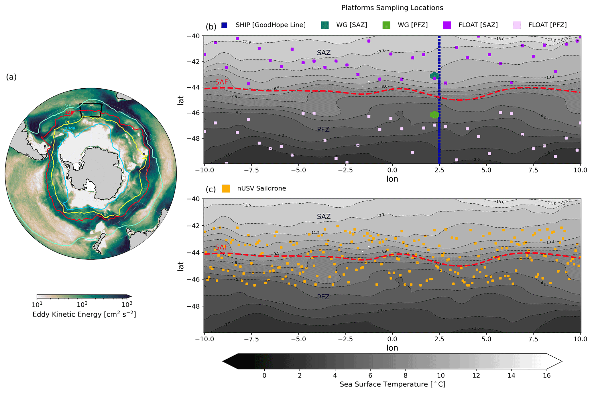
Figure 1 Panel (a) is the regional view of the BIOPERIANT12 model simulations with the selected experimental domain (black box) within the annual mean of the Southern Ocean major fronts and the changing conception of the Antarctic Circumpolar Current (ACC), showing the mean annual of eddy kinetic energy (EKE) derived from the model. From the north to south are the mean locations of the named fronts: the subtropical front (STF), the sub-Antarctic front (SAF), the polar front (PF), and the southern boundary (SBdy) front (based on Orsi et al., 1995). Colours show the EKE, illustrating the strong steering of the fronts. Panel (b) shows the map of the SST in the experimental domain (black box in Fig. 1a), on which are also shown the idealized sampling tracks/locations of the synthetic ocean observing platforms, SHIP, FLOAT, and WG as described in the figure legend. Panel (c) shows the sampling tracks of the idealized new unmanned surface vehicle (nUSV) Saildrone within the experimental domain. These locations, marked and coloured according to each corresponding sampling platform, are where we sample the BP12 model data in a way that is comparable to the real world. The SAF is characterized by the red line (Fig. 1a) and dashed red line (Fig. 1b–c), and it separates the experimental domain into the sub-Antarctic zone (SAZ) and polar frontal zone (PFZ).

This study was designed as a semi-idealized observing system simulation experiment (OSSE) to minimize some of the potential confounding factors in the final estimation of the root mean square error (RMSE), mean absolute error (MAE), and temporal and spatial biases while evaluating the performance of regression models used to extrapolate surface ocean pCO₂ values. A key part of this design was to remove the normal step of clustering that is necessary to overcome the spatial and temporal limitations of observations on a large-scale mapping domain (Fay and McKinley, 2013, 2014; Gregor et al., 2019; Landschützer et al., 2014). Thus, to avoid the clustering step, we chose a domain in the high-resolution (± 10 km) BP12 forced ocean biogeochemical model that was not only spatially and temporally coherent but also big enough to reflect the spatial and temporal scales necessary to provide sufficient sensitivity to the different sampling strategies. The selected domain, 10^∘ of latitude (40–50^∘ S) and 20^∘ of longitude (10^∘ W–10^∘ E) as depicted in Fig. 1a, is in the Atlantic sector of the Antarctic Circumpolar Current (ACC) between the subtropical front (STF) and the polar front (PF) and spans across the sub-Antarctic front (SAF) (Fig. 1a). Furthermore, the domain lies within the sub-polar seasonally stratified (SPSS) biome (Fay and McKinley, 2014). The Good Hope repeat hydrography sampling line passes through the domain (Fig. S1), for which sustained annual to bi-annual ship-based observations have been carried out for over a decade, as well as high-resolution carbon glider observations (Monteiro et al., 2015). More specifically, as shown in Fig. 1, our selected domain is crossed by the SAF and, therefore, includes the SAZ and the PFZ, inspired by Gray et al. (2018) and Chapman et al. (2020). The SAZ and PFZ, separated by the SAF (red line Fig. 1a and dashed red curve in Fig. 1b–c), are referred to as the north and south, respectively, of the experimental domain.

The oceanographic context of this domain is shown in Fig. 1a, depicting the selected 10^∘-by-20^∘ domain (black box) in the context of the Southern Ocean major fronts and the eddy kinetic energy (EKE) derived from the BP12 model. This confirms that the domain spans the sub-Antarctic front (SAF) and is in a region of relatively high or medium EKE.

2.3.2 Model vs. data products: the mean seasonal cycle of pCO₂

The mean seasonal cycles of pCO₂ reconstructions from two well-known machine-learning-based products (Landschützer et al., 2016; Gregor et al., 2019) are explored here within the study sub-domain in comparison with the BP12 model pCO₂ (Fig. 2). In the Southern Ocean, the observed maximum positive anomaly in surface ocean pCO₂ in winter (July–September) is linked to mixed-layer deepening and associated entrainment, while the maximum negative anomaly in summer is linked to the spring–summer net primary production (Gregor et al., 2018; Takahashi et al., 2009).

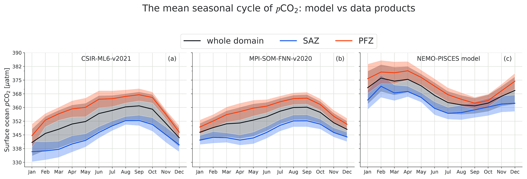
Figure 2 The mean seasonal cycle (SC) for surface ocean pCO₂ from two observation-based products and a high-resolution (± 10 km) forced NEMO-PISCES ocean model (BIOPERIANT12) within the selected experimental domain (Fig. 1a). The figure contrasts the respective seasonal cycles of the two observation-based products and the ocean model. Panels (a) and (b) show the mean SCs of the pCO₂ estimates from the two data products, CSIR-ML6-v2021 (Gregor et al., 2019) and MPI-SOM-FNN-v2020 (Landschützer et al., 2016), respectively, in the whole domain, the SAZ, and the PFZ; and similarly, panel (c) shows the mean SCs of the pCO₂ from the BIOPERIANT12 model.

The BP12 model sub-domain (black box, Fig. 1a) is depicted as a winter-maximum and summer-minimum pCO₂ area by both data products (Gray et al., 2018; Keppler and Landschützer, 2019) as shown in Fig. 2a–b. Thus, the domain-mean seasonal cycles of pCO₂ from these two products are quite consistent with the broader Southern Ocean (Gregor and Gruber, 2021). This is in sharp contrast with the seasonal cycle climatology from the high-resolution forced ocean model used in this study (Fig. 2c). The basis for this difference is that the high-resolution forced ocean model has a seasonal cycle that is largely influenced by the annual cycle of SST (Fig. 2c). This kind of temperature-driven model bias for surface ocean pCO₂ is now well recognized in both forced and coupled models in the Southern Ocean (Mongwe et al., 2016, 2018), but this study is more concerned with the modes of variability than it is with the mechanisms within the model. The forced coupled ocean model (NEMO-PISCES) represents the processes that regulate CO₂. However, for the purpose of this study, the “correctness” of the pCO₂ response to the driver variables does not really matter because here we examine the sensitivity of the reconstruction to how the sampling scales match the modes of variability.

2.3.3 Synthetic ocean observing platforms

In designing the sampling scales and strategies we opted to constrain the experiment to realistic and existing observing platforms that can make direct $p{\mathrm{CO}}_{\mathrm{2}}^{\mathrm{ocean}}$ or derived (from pH) surface ocean CO₂ observations. More specifically, the existing ocean observing platforms involved in these experiments are the ships (serving as the baseline) and the autonomous unmanned surface vehicles (USVs) – carbon floats, Wave Gliders, and Saildrones (the new USV) – whose simulations are dubbed SHIP, FLOAT, WG, and nUSV, respectively (Fig. 1b–c). The first autonomous platform, the carbon float, characterizes the autonomous profiling biogeochemical float operating in the Southern Ocean (Majkut et al., 2014; Williams et al., 2017; Gray et al., 2018). Manufactured by Teledyne Webb Research or Sea-Bird Electronics, these floats are designed to provided year-round measurements at 10 d periods (Johnson et al., 2017). The second autonomous platform, Wave Glider, is an autonomous USV developed by Liquid Robotics Inc (Sunnyvale, California, USA), which is unique in its ability to harness ocean wave and solar energy for platform propulsion (Hine et al., 2009). At sea it operates individually or in fleets, delivering real-time data for several months without servicing (Grare et al., 2021; Sabine et al., 2020). Equipped with physical and biogeochemical instruments/sensors, the Wave Glider gathers ocean data in ways or locations that were previously either too costly or challenging to operate in. Made by Saildrone Inc (Alameda, California, USA), the nUSV Saildrone is an autonomous ocean-going data collection platform navigable via satellite communications and designed for long-range, long-duration missions of up to 12 months (Gentemann et al., 2020; Meinig et al., 2016, 2019). It is predominantly powered by wind and solar energy and equipped with meteorological, ocean physical, and biogeochemical sensors for long-range ocean data collection missions (Gentemann et al., 2020) through remote surveying in the toughest of ocean environments such as the Southern Ocean (Meinig et al., 2019; Sutton et al., 2021).

Each of these simulated ocean observing platforms had a sampling routing through the domain that closely approximated reality. Ship-based sampling is along a single meridional repeat line (longitude), where repeats could be seasonal and annual (Fig. 1b). Floats followed a zonal sampling distribution that is consistent with the flow of the ACC and a 10 d sampling scale with a limited random meridional mesoscale variability which reflects the eddy kinetic energy (EKE) characteristics of the domain but is constrained by the SAF (Fig. 1a–b). Wave Gliders were constrained to repeat the pseudo-mooring sampling (± 20 km range) on the ship line (Fig. 1b), which captures the sub-mesoscale gradients but with a high temporal sampling frequency of 1 h. Moreover, from a logistic perspective, WGs were given a mooring-like sampling programme to ease their deployment and retrieval, for example, from the research vessel SA Agulhas II, which crossed the domain at the Good Hope line, whereas nUSVs were able to sail to the next port.

2.3.4 Idealized experiment setup

In this paragraph, we briefly describe the experimental scenarios shown in Table S2. We stress again the fact that these experiments are intentionally made to reproduce the sampling resolutions of their real-world counterparts, not necessarily the spatial resolution in practice but at least the temporal one. We considered the NEMO-PISCES model simulations, BP12, a realistic representation of the real ocean climate systems within which the $p{\mathrm{CO}}_{\mathrm{2}}^{\mathrm{ocean}}$ is known across the entire experimental domain. Based on this, we ask the following question: given measurements of $p{\mathrm{CO}}_{\mathrm{2}}^{\mathrm{ocean}}$ as sampled in a real-world scenario by these ocean observing platforms, how sensitive are the sampling distribution and resolution to observation-based estimates of $p{\mathrm{CO}}_{\mathrm{2}}^{\mathrm{ocean}}$ at every point across the entire experimental domain?

In these experiments, we simulate the sampling tracks/patterns of the synthetic ocean observing platforms SHIP, FLOAT, WG, and nUSV Saildrone (Fig. 1b–c). We leverage these synthetic sampling systems to sample the BP12 model data inside our selected experimental domain by constraining the experiment to their realistic and existing counterparts. The BP12 model sampled data from each of the sampling scenarios are then used for training and testing of the ML algorithms. The trained ML models are used to reconstruct the $p{\mathrm{CO}}_{\mathrm{2}}^{\mathrm{ocean}}$ values of the full experimental domain and compared with original BP12 model field $p{\mathrm{CO}}_{\mathrm{2}}^{\mathrm{ocean}}$ to assess the anomalies in reconstructed mean annual and seasonal cycles.

The idealized ship operates according to the sampling scales and strategies of ships involved in the SOCAT collaborative effort. However, here we considered the three following seasonal sampling regimes for the ship platform: (1) summer only, (2) winter and summer, and (3) autumn and spring. Like the real-world scenario, the ship simulation served as our baseline. The idealized carbon float simulates the SOCCOM biogeochemical float with a 10 d sampling cycle. Talley et al. (2019) reported the importance of the water masses and frontal structures in the deployment strategy of autonomous sampling platforms, such as floats, that will likely follow the fronts with an eastward trajectory but will seldom cross the front. Therefore, we consider the situation where the idealized floats do not cross the SAF as illustrated in Fig. 1b, even though in reality this might happen due to the occurrence of events such as storms or eddies. We thus considered two deployment and sampling scenarios to not disadvantage the floats and to value their large spatial structure: (1) in the SAZ and (2) in the PFZ (Fig. 1b). Given the pseudo-Lagrangian sampling patterns of an Argo float whose motion is driven by the water current, we assume that our idealized float moves eastwards and on a trajectory that is a Brownian motion or, more specifically, a random walk (Fig. 1b). The idealized Wave Glider operates according to the sampling strategies of the Wave Gliders used in the SOSCEx project (see Sect. S1.1 for additional details). Like the idealized float, we considered two deployment stations, the first in the SAZ (see Fig. 1b, hexagonal patterns in dark green) and the second in the PFZ (see Fig. 1b, hexagonal patterns in light green). This idealizes the two deployment scenarios of SOSCEx III gliders (cf. Fig. S1, hexagonal patterns in blue-yellow) that sampled on an hourly basis. However, given that the model temporal resolution is daily, our idealized Wave Glider samples daily. Lastly, we add an idealized Saildrone that simulates the sampling strategies of its real-world counterpart that can sample ocean data collection missions for up to 12 months (Gentemann et al., 2020; Meinig et al., 2019). As with the idealized Wave Glider, the Saildrone also samples daily. Further, we assume that by leveraging its speed the Saildrone sampling can be done across an ocean front, such as the SAF as depicted in Fig. 1c – a realistic assumption because in reality nUSV Saildrones sample at a much higher frequency (hourly) and can be piloted remotely (Gentemann et al., 2020; Sutton et al., 2021). We assumed that all three autonomous sampling platforms sampled year round in our experimental domain.

The observing system simulation experiment (OSSE) with nUSV Saildrone is inspired by the study of Sutton et al. (2021), which used nUSV to sample at a very high resolution and completed in about 6 months the first autonomous circumnavigation of Antarctica, providing hourly observations. At this frequency, the nUSV sampling density in this study domain (Fig. 1c) is realistic due to the size of the sampling domain. We extracted a subset of the Sutton et al. (2021) USV dataset within the sub-domain to obtain the USV tracks (cf. Fig. S6) and found that the Sutton et al. (2021) USV would take ∼ 16 d to cover our 20^∘ W–E domain, which corresponds to 16 × 24 h = 384 hourly samples. However, our nUSV sampling pattern (Fig. 1c) is idealized, with the goal of sampling across the sub-domains on both sides of the front (SAF), that is, in the SAZ and PFZ. By using a back-of-the-envelope approach, we find that the Saildrone would be able to cover our domain in 45 d using a zigzag pattern – assuming 42–46^∘ S with each pass covering 2.5^∘ W–E for each pass (∼ 500 km) with eight passes in our domain (4000 km) at a speed of ∼ 2 kn (∼ 3.7 km h⁻¹).

In summary, we sample the $p{\mathrm{CO}}_{\mathrm{2}}^{\mathrm{ocean}}$ and drivers using these above-mentioned synthetic sampling platforms, i.e. SHIP, FLOAT, WG, and nUSV Saildrone (Fig. 1b–c). We emphasize that these experiments are intentionally made to reproduce the sampling resolution of their real-world counterparts, not necessarily their spatial resolution in practice but at least the temporal one. Then we use ML regression techniques to reconstruct the full experimental domain and compare it with the BP12 model truth $p{\mathrm{CO}}_{\mathrm{2}}^{\mathrm{ocean}}$ in the full domain to assess the reconstructions as anomalies of mean annual and seasonal cycles, which is a key objective of this work.

2.4 Machine learning implementation

We use a two-member ensemble method (we call ML2) that consists of two state-of-the-art ML approaches: the feed-forward neural network (FNN) and a variant of gradient boosting decision tree (GBDT) learning frameworks called gradient boosting machines (GBMs). Our choice of FNN method is motivated by its recent success in approximating the surface ocean pCO₂ (Denvil-Sommer et al., 2019; Gregor et al., 2019; Landschützer et al., 2013, 2016). The choice of the GBDT approach is motivated by its achievement of state-of-the-art performances in many ML tasks (Ke et al., 2017) and also the success of previous GBDT approaches (Gloege et al., 2021; Gregor et al., 2019; Gregor and Gruber, 2021). We use the scikit-learn and LightGBM Python packages for our implementation of FNN and GBM, respectively. We thus focus here only on the ensemble average ML2, whose stacking process is illustrated in Fig. 3a. Unlike the two main techniques of reference (Landschützer et al., 2016; Gregor et al., 2019), both of which include a clustering step, in this study we avoided it because of the size of the study domain (10^∘ of latitude, 40–50^∘ S, by 20^∘ of longitude, 10^∘ W–10^∘ E). More details of our motive for skipping this step are provided in Sect. S2.3.

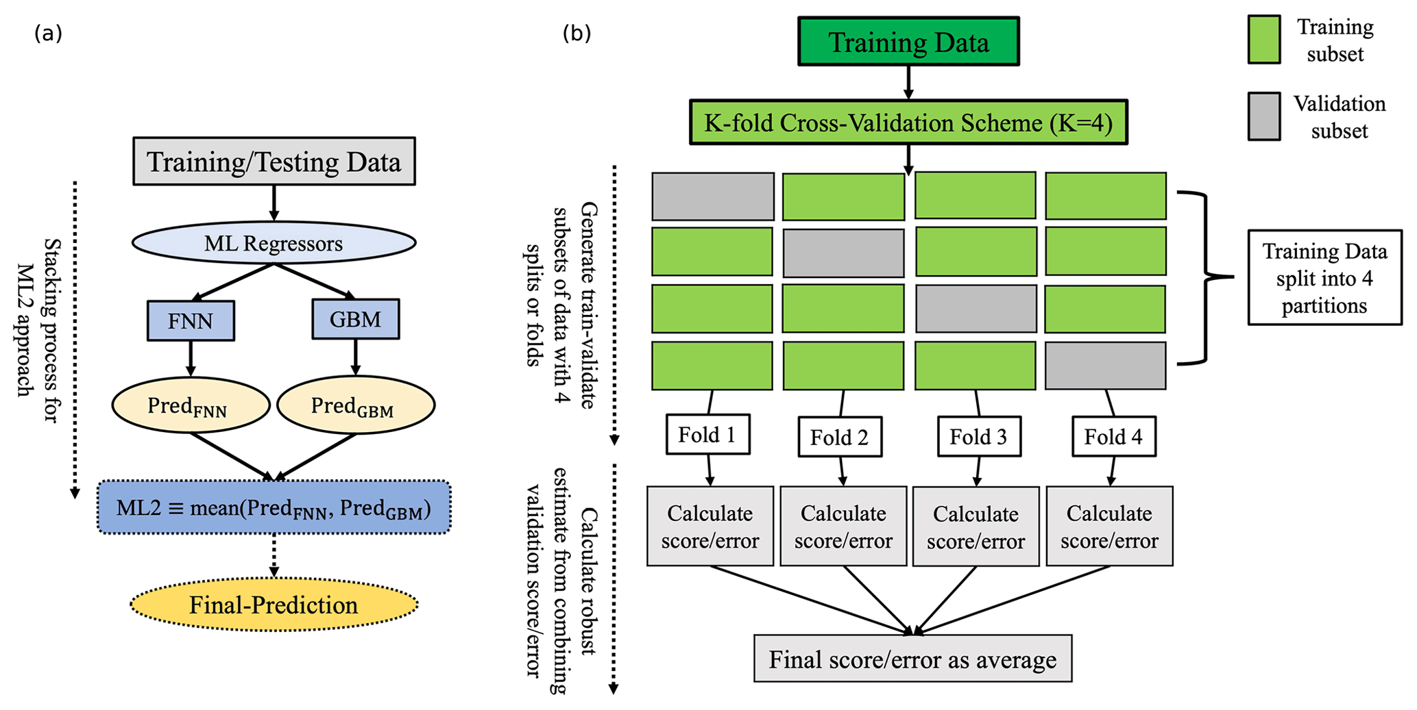
Figure 3 Schematic flow diagram of the two-member ensemble method ML2. Panel (a) shows the schematic representation of the stacking process of the two machine learning (ML) algorithms, FNN and GBM, that make up ML2; panel (b) shows the schematic flow diagram of the K-fold cross-validation (CV) procedure used in hyper-parameter optimization (HOP) of the two members (FNN, GBM) of ML2. To extrapolate from surface ocean pCO₂ samples, ML2 uses full domain coverage model data of the predictor variables SST, SSS, MLD, and Chl a. These variables serve as proxies for known processes that affect surface ocean pCO₂ (Takahashi et al., 1993).

Given that the observation size is relatively small, especially for the baseline experiment (SHIP summer only), immediately splitting the simulated data into training and testing sets may not capture some key features of the original platform observations. We thus use the entire sampled data for model building instead of splitting the data into two sets. As shown in Fig. 3b, however, to control the overfitting, we incorporate a K-fold cross-validation (CV, with K=4) during the model training in order to find the set of hyper-parameters that enable a better generalization of ML2. Like in Gregor et al. (2019), the CV is applied identically to each of the two-member algorithms (FNN and GBM) except that here, the tuning of hyper-parameters was achieved using a Bayesian-search CV (BayesSearchCV) instead of a grid-search CV. We make use of the scikit-optimize Python package for our BayesSearchCV implementation. The optimal values of ML2 hyper-parameters used were reported at the end of the training and are included in the Supplement (Tables S4 and S5) for reproducibility. Further, the testing of generalization is done through quantitative comparison of the estimates with model data (known truth) that were not involved in the simulations of synthetic platforms.

2.5 Machine learning regression metrics

Although the choice of the performance measure may seem straightforward and objective, it is often difficult to choose a metric that corresponds well to the desired behaviour of the ML algorithm (Goodfellow et al., 2016). The reconstruction power of the surface ocean pCO₂ of the full experimental domain is thus estimated using a series of four statistical metrics that include the mean bias error (MBE), mean absolute error (MAE), root mean square error (RMSE), and Pearson's correlation coefficient (r) to measure the tendency or strength of estimates and observations to vary together (Stow et al., 2009) or, more technically, to quantify the level at which reconstruction captures the phasing observed in the model truth (Gloege et al., 2021).

The MBE, commonly called bias, is the mean difference between the estimates and the target variable samples. It captures the average bias/error in the predictions and is calculated as follows:

$$\begin{array}{}\text{(2)}& \mathrm{MBE}={\displaystyle \frac{\mathrm{1}}{n}}{\sum }_{i=\mathrm{1}}^n\left({\widehat{y}}_i-y_i\right),\end{array}$$

where n is the number of samples, $\widehat{y}$ is the model prediction, and y is the target variable (in this case, $p{\mathrm{CO}}_{\mathrm{2}}^{\mathrm{ocean}}$).

The MAE denotes the ratio of the L1 norm of the error vector to the number of samples (n). More specifically, the MAE derives from the unaltered magnitude (or absolute value) and provides an estimate of the average magnitude of the error. It is calculated as follows:

$$\begin{array}{}\text{(3)}& \mathrm{MAE}={\displaystyle \frac{\mathrm{1}}{n}}{\sum }_{i=\mathrm{1}}^n\left|{\widehat{y}}_i-y_i\right|.\end{array}$$

The RMSE, one of the most popularly used metrics in the climatic and environmental sciences community when dealing with regression modelling problems, is also a measure of the difference between the estimates ${\widehat{y}}_i$ and the target variable samples y_i. It provides an estimate of the variability in the predictions in terms of the fitness with the observed data and is defined as follows:

$$\begin{array}{}\text{(4)}& \mathrm{RMSE}=\sqrt{{\displaystyle \frac{\mathrm{1}}{n}}{\sum }_{i=\mathrm{1}}^n{\left({\widehat{y}}_i-y_i\right)}^{\mathrm{2}}}=\sqrt{\mathrm{MSE}},\end{array}$$

where MSE is simply the mean square error. For squaring individual errors $e_i={\widehat{y}}_i-y_i$ ($i=\mathrm{1},\mathrm{\dots },n)$, the stated rationale is usually to “disconnect the sign” of e_i so that the magnitudes of errors influence the average error, MSE.

In order to quantify the strength of the linear association between the $p{\mathrm{CO}}_{\mathrm{2}}^{\mathrm{ocean}}$ estimates (i.e. ${\widehat{y}}_i$ for in) and observations/known truth (i.e. y_i for $i=\mathrm{1},\mathrm{\dots },n)$, Pearson's correlation coefficient (r) is used. Its computing is formulated as follows:

$$\begin{array}{}\text{(5)}& r={\displaystyle \frac{\mathrm{1}}{(n-\mathrm{1}){\mathit{\sigma }}_y{\mathit{\sigma }}_{\widehat{y}}}}{\sum }_{i=\mathrm{1}}^n\left(y_i-\stackrel{\mathrm{‾}}{y}\right)\left({\widehat{y}}_i-\stackrel{\mathrm{‾}}{\widehat{y}}\right),\end{array}$$

where σ_y and ${\mathit{\sigma }}_{\widehat{y}}$ are the standard deviations of y and $\widehat{y}$, respectively, and $\stackrel{\mathrm{‾}}{y}$ and $\stackrel{\mathrm{‾}}{\widehat{y}}$ the means of y and $\widehat{y}$, respectively. The correlation coefficient always takes values between −1 and 1, with lower (near −1) and higher (near 1) values of r indicative of how much reconstruction and model are in or out of phase, respectively. Values of r that are close to 0 are indicative of no association between the two signals. Therefore, the ideal value for r will be close to 1.

2.6 Uncertainty decomposition/breakdown

A firm understanding of the uncertainties is required for the purpose of our analysis given that in our study we are dealing with the uncertainties that we cannot fully quantify now as this is on unseen or out-of-sample data like in Gloege et al. (2021). Therefore, it is necessary to distinguish the different types of uncertainties. We assume that our sampled observations are unbiased, and hence the training datasets for surface ocean pCO₂ are considered as such known data; and this can be justified by the fact that we have access to all the data. The terms error and uncertainty are interchangeably used although here the latter is used as an estimate quantifiable against a known value, whereas the former characterizes a range of values within which the true value is asserted to lie with some level of confidence (Gregor and Gruber, 2021).

The pCO₂ total uncertainty (E) is dealt with as in Gregor and Gruber (2021). The authors identified three main sources of errors that contribute to E within the surface ocean carbonate system. These include the (1) measurement (M), (2) representation (R), and (3) prediction (P) errors. Under the assumption that these components are independent of each other in the pCO₂ total uncertainty space, E can thus equivalently be expressed as the norm of the vector whose coordinates are P, M, and R, that is, the square root of the sum of the squares of these components: $E=\sqrt{P^{\mathrm{2}}+M^{\mathrm{2}}+R^{\mathrm{2}}}$. We can remove the contribution of the measurement uncertainty from this equation since we are sampling from a synthetic dataset. Further, we address the representation uncertainty by sampling at a higher resolution (Gregor and Gruber, 2021). Given that we are predicting at high resolution ($\mathrm{1}/\mathrm{12}$^∘ daily), the sampling distribution bias due to capturing of large-scale gradients is assumed to be small since we are within the 2 d threshold set by Monteiro et al. (2015). Lastly, we assume that the ML models are the best possible predictors for the given training datasets, since each ML model was trained using best practices (i.e. low in-sample errors calculated from all the training points as shown in the Supplement). Therefore, reported RMSEs will be the uncertainties due to sampling bias.

3 Results

In the next sections, the results for the following four sets of semi-idealized model experiment combinations – SHIP, SHIP + FLOAT, SHIP + WG, and SHIP + nUSV – are presented in terms of spatial and seasonal cycle anomalies of the annual mean pCO₂ estimates.

3.1 Annual mean seasonal cycle for the domain

The annual mean map for pCO₂ (mean 368.15 µatm; standard deviation 50.5 µatm) shows that the domain is characterized by both meridional and mesoscale variability expected from the mesoscale-resolving BIOPERIANT12 model (Fig. 4a). The meridionally distinct SAZ (north of the domain) (<368.15 µatm) and PFZ (south of the domain) (>368 µatm) are separated by the sub-Antarctic front (SAF) (Figs. 1 and 4a). This mean map also highlights the importance of mesoscale gradients in both the SAZ and the PFZ domains (Fig. 4a). The mean seasonal cycles of pCO₂ for the whole domain as well as for the SAZ (lower – blue) and PFZ (higher – red) are depicted in Fig. 4b. It shows that the seasonal cycle of $p{\mathrm{CO}}_{\mathrm{2}}^{\mathrm{ocean}}$ is dominated by the influence of the annual cycle of the sea surface temperature (SST) on CO₂ solubility (Mongwe et al., 2016; Munro et al., 2015) with warm late summers (February–April) and cool late winters (July–September) (Fig. 4b). The three seasonal cycles (whole domain, SAZ, and PFZ) show coherence in the seasonal amplitude and phasing except that the warming transition from winter to spring occurs 2 months earlier (July) in the SAZ relative to the PFZ (Fig. 4b).

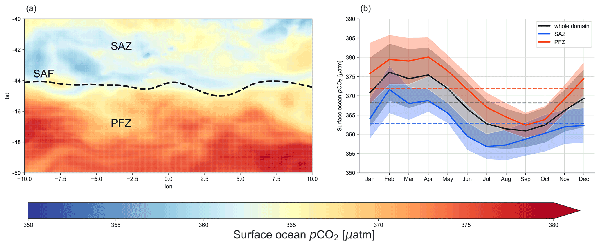
Figure 4 Characterization of the spatial and temporal surface ocean pCO₂ annual mean state within the selected 10^∘-by-20^∘ experimental domain located in the northern ACC that corresponds to the SPSS biome (Fay and McKinley, 2014) as shown in Fig. 1a. Panel (a) shows the map of mean annual pCO₂ from the BIOPERIANT12 (BP12) model. It shows that the domain is characterized by a regional meridional gradient including the sub-Antarctic front (SAF) (dashed black line) as well as mesoscale gradients in both the SAZ and the PFZ; panel (b) shows the mean seasonal cycles for surface ocean pCO₂ in the BP12 model domains (SAZ, SAF, and PFZ) where the dashed lines indicate the magnitude of the annual mean – for each domain – 368.16 µatm (domain), 362.85 µatm (SAZ), and 371.78 µatm (PFZ).

Notwithstanding the phasing differences, we still find a comparable winter reconstruction bias in this study (Figs. 2c and 4b) and observation-based products (Fig. 2a–b). Thus, the question is whether the magnitude of the reconstructed winter pCO₂ maximum is realistic or a result of the way the machine learning methods process the summer sampling bias in a system characterized by strong seasonal and intra-seasonal modes of variability.

3.2 Reconstructed mean annual spatial and seasonal cycle anomalies

In order to investigate the anomalies in the reconstruction of the mean annual and seasonal cycles, which comprise a key objective of this study, we first characterized the anomaly by the mean bias error (MBE) and calculated the MBE at each grid point of the spatial domain. Secondly, we also calculated the anomaly of the seasonal cycle reconstruction in each of the sub-domains. More specifically, we used the seasonal cycle residuals to explore how a systematic anomaly could influence the reconstruction of pCO₂ values at the surface ocean. We performed this calculation for each experiment and their respective reconstructions and also examined their spatial variability.

3.2.1 Semi-idealized SHIP-only observation experiment results

The semi-idealized SHIP-only sampling experiments mimic the largely ship-based SOCAT gridded product to evaluate the sensitivity of the reconstruction uncertainties (RMSE, MAE, MBE/bias) to seasonal meridional sampling scenarios. In each of these scenarios the ship makes two meridional crossings in opposite directions 1 month apart (Fig. 1b). This SHIP-only set of seasonal sampling experiments gives our baseline as it is also used in all platform combinations. Three seasonal sampling scenarios (summer (smr), summer + winter (smr + wtr), and autumn + spring (aut + spr)) were considered. While the first two scenarios are addressed in detail in this study (Fig. 5a–b and Table 1), the third one can be found in the Supplement (Fig. S5 and Table S6) in support of the main points already made in Fig. 5a–b.

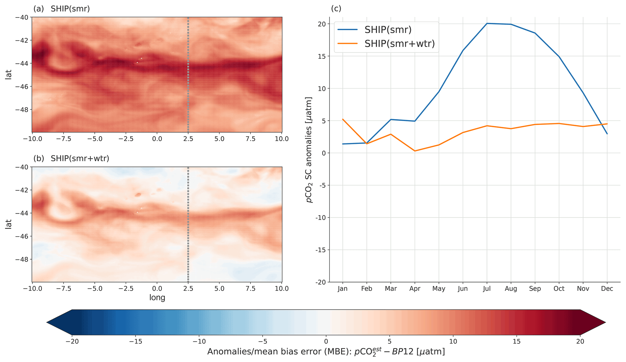
Figure 5 Reconstruction anomalies for the idealized SHIP experiment where the idealized ship sampled the domain based on the sampling regimes/scenarios SHIP(smr) for summer and SHIP(smr + wtr) for summer and winter. Panels (a) and (b) show the maps of the reconstruction anomalies according to the two sampling regimes SHIP(smr) and SHIP(smr + wtr), respectively; panel (c) shows the anomalies of the mean seasonal cycle (SC) reconstruction based on these two sampling regimes, that is, SHIP(smr) and SHIP(smr + wtr). The meridional dotted grey line in panels (a) and (b) illustrates the sampling line (summer and winter) and serves as a reminder of how SHIP sampling was performed.

The spatial and seasonal cycle anomalies from the reconstructions for the summer (smr) and summer and winter (smr + wtr) sampling lines are depicted in Fig. 5a–b. The results for the autumn and spring (aut + spr) sampling lines are summarized in the Supplement (Fig. S6). The uncertainties and regression errors for all three experiments are shown in Table 1. These results showed that the highest positive anomalies in the reconstruction of the mean and the seasonal cycle occur when a ship samples (i.e. makes two passes in consecutive months) the sub-domain only in summer (Fig. 5a, c). This sampling strategy resulted in a strong positive anomaly (± 20 µatm) that peaks in winter and weakens in mid-summer (Fig. 5c). In sharp contrast, when winter sampling crossings are added to the summer scenario (smr + wtr) the spatial and seasonal anomalies are significantly reduced from 20 to <5 µatm, respectively (Fig. 5b, c). The weaker but persistent positive anomaly in the SAF accounts for most of the reduced positive seasonal cycle anomaly (Fig. 5a, c).

All scenarios depict a mesoscale modulated positive annual pCO₂ anomaly (MBE) climatology in the vicinity of the SAF (Fig. 5a–b). However, this is slightly offset by equally strong positive anomalies in the SAZ and PFZ for the smr scenario (Fig. 5a), while the meridional gradients of the anomalies are much weaker for the smr + wtr scenario (Fig. 5b). These differences are very well reflected in the anomalies of their corresponding seasonal cycles (Fig. 5c).

Table 1 ML regression modelling scores of the ensemble average (ML2) for two sampling scenarios of the SHIP experiment: SHIP(smr) for summer sampling and SHIP(smr + wtr) for summer and winter sampling. The configuration of this set of experiments is presented in Table S2 and clearly described in Sect. 2.3.4. The first column of the table is the experimental set, and the second one corresponds to the considered experiments. The statistical metrics used to assess ML2 for this set of experiments are abbreviated as follows: RMSE is the root mean square error calculated following Eq. (4); MAE is the mean absolute error (Eq. 3); MBE or bias is the mean average error (Eq. 2); and r is Pearson's correlation coefficient (Eq. 5) between the reconstructed and BP12 model truth pCO₂. Values in the table are significantly different from the mean for the corresponding column (with a 95 % confidence level or p value < 0.05 for the two-tailed Z test).

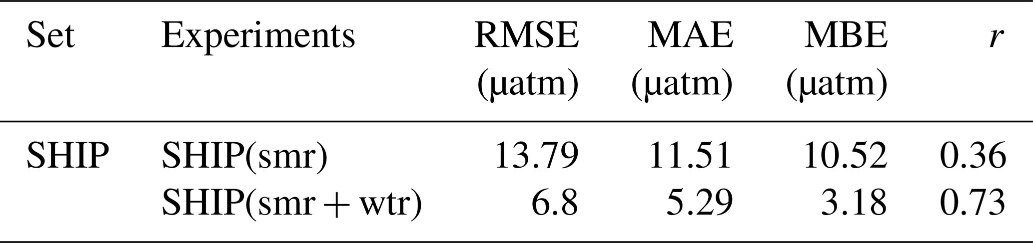
These SHIP-only experiment results (Tables 1 and S3) also show that the summer-only sampling of the sub-domain both produces the largest sampling bias (10.52 µatm, with an RMSE of 13.79 µatm) and yields the weakest correlation between the underlying pCO₂ estimates and the model ground truth (with r=0.36). On the other hand, they also show that if the ship undertakes just one more meridional voyage in winter, this halves the RMSE to 6.8 µatm and the bias (MBE) to 3.18 µatm compared to the summer-only sampling experiment, SHIP(smr). Moreover, they also strengthen the linear association between the reconstruction and BP12 model ground truth for pCO₂ (r=0.73).

3.2.2 Idealized SHIP and autonomous observations platform experiments

In this section, we present the results of three sets of combined ship and autonomous platform experiments (SHIP(smr) + FLOAT, SHIP(smr) + WG, and SHIP(smr) + nUSV) that allowed us to test the hypothesis that complementing summer biased ship-based sampling with year-long high-resolution sampling in space and time reduces the reconstruction uncertainties and positive annual mean and seasonal cycle biases relative to the ship sampling alone (Figs. 5a and c and 6a–b) (Bushinsky et al., 2019; Gregor et al., 2019; Sutton et al., 2021). We simulated and analysed the reconstruction of the mean annual pCO₂ and seasonal cycles from carbon floats (FLOAT) and carbon Wave Gliders (WG) deployed independently for a year in the sub-Antarctic zone (SAZ) and polar frontal zone (PFZ) (Fig. 6b, c, d, e, f). These were complemented by simultaneous year-round FLOAT deployments in the SAZ and PFZ (Fig. 6b, g) and a deployment of the new unmanned surface vehicle (nUSV) Saildrone that spanned across all three domains (Fig. 6b, h).

These results show that both the reconstructed mean annual anomaly and the seasonal cycle of pCO₂ are very sensitive to the spatial and temporal characteristics of the additional autonomous sampling platform (Fig. 6). Statistics (Table 2) show that all the autonomous platform deployment experiments improved the significant winter-positive-biased seasonal cycle anomaly from the summer ship sampling reconstruction (± 20 µatm). However there remained a small but variable (2–10 µatm) winter–spring seasonal bias in all deployment combinations (Fig. 6b). The exception was the experiment with a FLOAT deployment in the SAZ, which resulted in a negative seasonal bias that also peaked in winter (± 10 µatm) and started earlier in the autumn (Fig. 6b). The two experiments with the smallest seasonal biases were the SHIP(smr) + WG(SAZ) and SHIP(smr) + nUSV. The first, SHIP(smr) + WG(SAZ), showed a small negative bias in the summer (<−5 µatm) and a small positive bias in the winter (<5 µatm). The latter, SHIP(smr) + nUSV, showed a small positive bias in summer (0–5 µatm) and in winter (4–5 atm) (Fig. 6b). In contrast, the experiment SHIP(smr) + FLOAT(SAZ + PFZ) that combined the 2-year-round FLOAT deployments (SAZ and PFZ) shows a minimal bias in summer but among the highest for all the experiments in winter (± 10 µatm) (Fig. 6b).

The spatial annual mean pCO₂ experimental scenario anomalies are consistent with the characteristics of the seasonal cycle of pCO₂ (Fig. 6a, c–h). In all cases the sub-Antarctic front (SAF) emerged as a feature with a variable positive pCO₂ anomaly relative to the SAZ and PFZ sectors to the north and south, respectively (Fig. 6a, c–h). All the scenarios highlight significant mesoscale anomaly gradients across all the domains (Fig. 6a, c–h). The year-long deployment of FLOATs and WGs in the SAZ leads to negative anomalies in both the SAZ and the PFZ, but those for the WG experiments are significantly weaker (Fig. 6c, e).

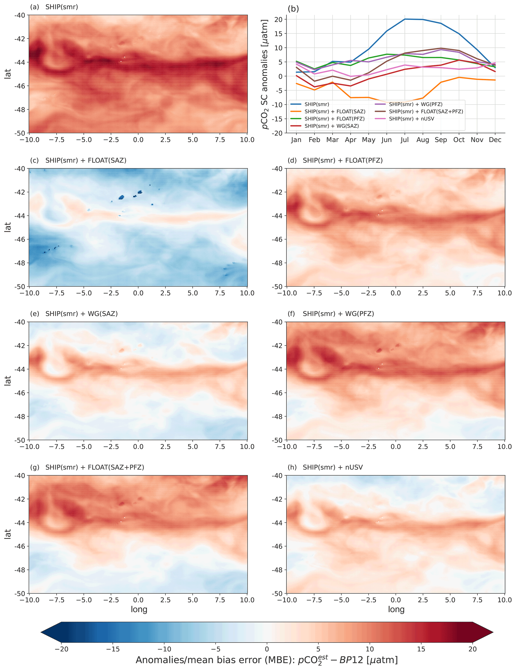
Figure 6 Reconstruction anomalies for the four sets of experiments, SHIP, SHIP + FLOAT, SHIP + WG, and SHIP + nUSV with a particular focus on the summer-only baseline scenario: SHIP(smr). Panel (a) shows the spatial anomalies or biases (MBEs) of the mean annual pCO₂ reconstruction for the SHIP summer-only sampling scenario, that is, SHIP(smr); panel (b) shows the anomalies of mean seasonal cycle (SC) reconstructions of the summer-only sampling scenario of the above-mentioned sets of experiments; panels (c) and (d) show the spatial reconstruction anomalies for the SHIP + FLOAT experiments, where two independent FLOATs were deployed in the SAZ and PFZ (respectively), and is used to supplement SHIP(smr); panels (e) and (f) show the spatial reconstruction anomalies for the SHIP + WG experiments, where two independent WGs were deployed along the SHIP line in the SAZ and PFZ (respectively), and is used to supplement SHIP(smr); panel (g) shows the spatial anomalies of the mean annual pCO₂ reconstruction for the SHIP + FLOAT experiment scenario where the two FLOAT deployments (SAZ and PFZ) were used to supplement the SHIP summer-only sampling scenario, hence SHIP(smr) + FLOAT(SAZ + PFZ); and panel (h) shows the spatial anomalies of the mean annual pCO₂ reconstruction for the SHIP + nUSV experiments where SHIP(smr) were supplemented by a year-round sampling of the nUSV Saildrone, hence SHIP(smr) + nUSV.

However, the reverse was found for the SAF zone, which shows a stronger positive anomaly for the WG(SAZ) than for the FLOAT(SAZ) (Fig. 6c, e). The stronger mean annual negative pCO₂ anomaly for the SHIP(smr) + FLOAT(SAZ) deployment is consistent with the negative seasonal cycle anomaly, which points to the mean annual anomaly being mainly influenced by the winter-negative anomaly (Fig. 6b–c). Similarly, the much weaker negative anomalies in the SAZ and PFZ for the WG deployment are consistent with the weaker seasonal cycle (<± 5 µatm) of pCO₂ for the whole domain.

SHIP(smr) + FLOAT(PFZ) and SHIP(smr) + WG(PFZ) deployments result in weak to moderate positive anomalies in the northern half of the PFZ, the SAZ, and the SAF and weak to zero anomalies in the southern PFZ, all of which are characterized by mesoscale gradients (Fig. 6d, f). Both scenarios show a comparable positive seasonal cycle anomaly although the phasing of the winter maximum is earlier, June vs. September, for SHIP(smr) + FLOAT(PFZ) (Fig. 6b). The mean annual pCO₂, from the combined SHIP(smr) + FLOAT(SAZ + PFZ) deployments, showed spatial characteristics similar to those of SHIP(smr) + FLOAT(PFZ) but with intensified negative and positive anomalies in the PFZ and SAZ, respectively (Fig. 6g). The moderately strong positive winter anomalies (± 10 µatm) in the seasonal cycle for this experiment indicate that the mean annual positive anomalies are also dominated by the winter anomalies (Fig. 6b). The mean annual pCO₂ anomaly for the SHIP(smr) + nUSV deployments is weakly negative (<−5 µatm) in the north SAZ and weakly positive (<5 µatm) in the SAF and the PFZ (Fig. 6h). The overall weak mean annual pCO₂ anomaly is consistent with the weakest (0–5 µatm) seasonal cycle anomaly (Fig. 6b).

Table 2 ML regression modelling scores of the ensemble average (ML2) for the summer-only sampling scenario (smr) of all the four sets of experiments: SHIP, SHIP + WG, SHIP + FLOAT, and SHIP + nUSV. The configuration of these experiments is presented in Table S2 and described in Sect. 2.3.4. Similarly to Table 1, the first column of the table is the experimental set and the second one corresponds to the considered experiments. The statistical metrics used to assess ML2 for this set of experiments are abbreviated as follows: RMSE is the root mean square error calculated following Eq. (4); MAE is the mean absolute error (Eq. 3); MBE or bias is the mean average error (Eq. 2); r is Pearson's correlation coefficient (Eq. 5) between the reconstructed and the BP12 model truth pCO₂. Values in the table are significantly different from the mean for the corresponding column (with a 95 % confidence level or p value < 0.05 for the two-tailed Z test).

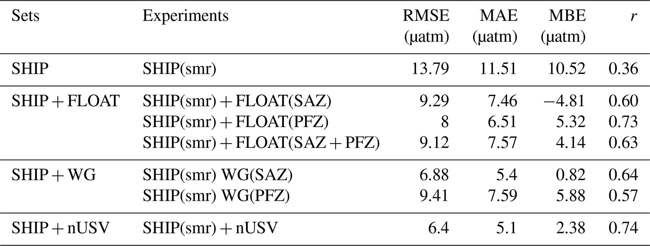
Table 2 shows that SHIP(smr), the baseline-biased ship summer sampling experiment (the status quo in the Southern Ocean), yielded an RMSE of 13.79 µatm and a mean biased error of 10.52 µatm, which is comparable with the Southern Ocean results for CSIR-ML6 (Gregor et al., 2019). Table 2 also shows that although all the additional high-resolution platform experiments reduced the RMSE and MBE, the magnitude of the impact was very sensitive to the platform and its location. All three scenarios of the year-long SHIP(smr) + FLOAT experiments reduced the RMSE of the SHIP(smr) experiment by 32.6 %–41.9 %; however, only the scenario SHIP(smr) + FLOAT(PFZ) provided the lowest RMSE and MAE as well as statistically significant correlation (r=0.73) between the estimates and known truth. Both WG experiments (SAZ and PFZ deployments) also reduced the RMSE by 31.7 %–50.1 % through a statistically significant correlation with r = 0.64 (SAZ) and r=0.57 (PFZ), respectively (Table 2). The SHIP(smr) + nUSV experiment yielded the lowest RMSE (6.4 µatm) (53.5 %), MAE, and MBE with a significant correlation with r=0.74. These results are consistent with the comparative seasonal cycle anomalies that showed SHIP(smr) + FLOAT(PFZ) and SHIP(smr) + nUSV to have the smallest seasonal cycle biases (Fig. 6b) and higher correlations with the known truth (with r=0.73 and r=0.74, respectively).

4 Discussion

Resolving the variability and trends of the seasonal cycle of pCO₂ in the Southern Ocean has been a long-term objective for the ocean carbon community to reduce the uncertainties and biases in the seasonal and mean annual fluxes (Bushinsky et al., 2019; Gregor et al., 2018; Lenton et al., 2006, 2013; Mongwe et al., 2018; Monteiro et al., 2015; Sutton et al., 2021; Takahashi et al., 2009). This started with largely observation-based approaches which constrained the seasonal cycle climatology (Takahashi et al., 2009, 2012) and set requirements to resolve the variability (Lenton et al., 2006; Monteiro et al., 2015). The advent of globally coordinated surface ocean CO₂ data, SOCAT (Bakker et al., 2016), together with machine learning methods (Landschützer et al., 2014, 2016; Rödenbeck et al., 2015) provided a basis for spatial and temporal gap filling that has resulted in an internally consistent set of reconstructions for the ocean and Southern Ocean CO₂ fluxes that contribute to the global carbon budget (Canadell et al., 2021; Fay et al., 2021; Friedlingstein et al., 2021).

However, Gregor et al. (2019) argued that the uncertainties and biases in CO₂ flux reconstructions are now limited by both data gaps and variability-scale sensitivity of surface ocean CO₂ observations – a boundary that the authors dubbed “the wall”. Our results make the key point that the seasonal and mean annual biases and uncertainties (RMSEs) in the reconstructions depend critically on simultaneously resolving the spatial, meridional gradients and temporal, seasonal, and intra-seasonal variability. We now discuss three sampling-scale sensitivities emerging from our analysis and what we suggest is required to get “over the wall”: (1) the sensitivity of the reconstructions to the seasonal cycle, (2) the sensitivity of the reconstructions to the seasonal cycle of the meridional gradients, (3) the sensitivity of the reconstructions to the intra-seasonal variability, (4) the need to simultaneously sample the meridional gradients and their intra-seasonal variability to get over the wall, and (5) the limitations of this study.

4.1 Seasonal sampling-scale sensitivity

The SHIP-only sampling experiments, which most closely simulate the historical ship-based and seasonally biased SOCAT gridded database in the Southern Ocean, point towards an unexpectedly high sensitivity of the reconstruction uncertainties and biases to the seasonal sampling scales (Figs. 1b and 5a–b, and Table 1). Simulation of the existing Southern Ocean ship summer sampling, SHIP(smr), resulted in a seasonal cycle reconstruction with a strong positive winter outgassing seasonal anomaly bias of ± 20 µatm that was strong enough to reverse the ingassing flux from the model domain (Fig. 5c) and also biased (positively) the spatial mean annual flux for the domain (Fig. 5a). The impact of the biased summer sampling is also expressed in the comparatively elevated RMSE, 13.79 µatm (Table 1), which is of a magnitude close to the RMSEs of the ML methods for the Southern Ocean – particularly in the polar frontal zone (PFZ). For example, Gregor et al. (2018) reported in the PFZ an average RMSE value of 14.33 µatm and also RMSE = 13.09 µatm for the SOM-FNN method (Landschützer et al., 2016) within the same region (PFZ). Furthermore, a comparative analysis of the SHIP summer-only experiment, SHIP(smr), and the SHIP summer and winter one, SHIP(smr + wtr), shows that SHIP(smr + wtr) outperformed SHIP(smr) across all the performance metrics (Table 1) by halving them; for instance, RMSE = 6.88 µatm. The sensitivity of the reconstruction to the seasonal sampling bias is again further emphasized by the impact of the addition of a single SHIP meridional two-leg winter (July–August) sampling line, SHIP(smr + wtr), which reduced the mean monthly winter anomaly of pCO₂ for the whole domain from ± 20 µatm in winter to less than 5 µatm over the whole seasonal cycle (Fig. 5a–c). The impact of the additional winter line is also expressed in the reduction in the bias error from Table 1.

When splitting the anomalies across the two sub-domains (SAZ and PFZ) for the SHIP(smr) scenario, a comparable seasonal sampling bias sensitivity was found for the SAZ and PFZ domains (Fig. 7a). The winter reconstruction bias dominates any internal variability in the sub-domains. However, the introduction of the SHIP winter line not only impacted on the overall mean seasonal bias but also shows that the mean seasonal cycle comprises out-of-phase seasonal modes of variability in both the SAZ and the PFZ domains (Fig. 7b).

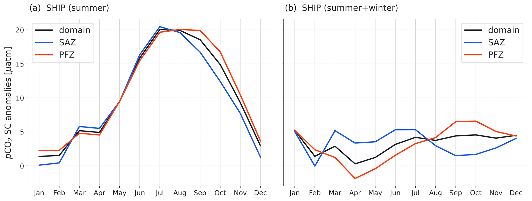
Figure 7 Anomalies of the mean surface ocean pCO₂ seasonal cycle (SC) reconstructions from two SHIP-only experiments. Panel (a) shows the pCO₂ SC anomalies from the SHIP (summer-only) reconstruction in the whole domain, the SAZ, and the PFZ; and in contrast, panel (b) shows the pCO₂ SC anomalies from the SHIP (summer + winter)-based reconstruction for the whole domain, the SAZ, and the PFZ.

It suggests that an important outcome of the reduction in seasonal and mean biases is the emergence of important modes of variability that can provide a useful window into key processes as well as into identifying key modes of variability that can influence sampling strategies (Fig. 7a–b). Our findings on the sampling bias sensitivity are consistent with the early estimates of the minimum number of ship transects required to observationally resolve the seasonal cycle in the Southern Ocean being quarterly, across the four seasons, and zonally 30^∘ apart (Lenton et al., 2006; Monteiro et al., 2010). Together with these early results, our analysis confirms that additional ship pCO₂ observation lines in summer will not be a useful contribution towards reducing the uncertainties and biases in the reconstructions. Rather, as proposed earlier, additional seasonal sampling lines in winter will make a decisive impact (Figs. 5a–c and 7a–b and Table 1). However, realistically this is not achievable because access to the Southern Ocean outside the summer period is logistically challenging outside the Drake Passage (Gray et al., 2018; Monteiro et al., 2015).

The well-recognized seasonal sampling bias problem, outside the Drake Passage (Munro et al., 2015), is being addressed globally and in the Southern Ocean using a variety of autonomous sampling platforms such as Wave Gliders, pH floats, and Saildrones (Bushinsky et al., 2019; Gray et al., 2018; Monteiro et al., 2015; Sutton et al., 2021; Williams et al., 2017). We now discuss the effectiveness of each one through experiments to simulate their sampling characteristics inside the model domain. All these experiments include the SOCAT-like SHIP summer observations. These experiments focus primarily on the impact of the autonomous sampling platforms WG and pH floats as both have been deployed in the Southern Ocean with sampling strategies that seek to address the seasonal sampling bias (Gray et al., 2018; Gregor et al., 2019; Monteiro et al., 2015). We return to the potential of Saildrones later in the discussion in the context of how to get over the wall.

4.2 The seasonal cycle of the meridional gradients

One of the unexpected results from our analysis was that the ship-based reconstruction with both summer and winter crossings of the domain, SHIP(smr + wtr), performed as well as the best reconstructions in which the SHIP summer-only sampling, SHIP(smr), is supplemented with an autonomous WG vehicle or FLOAT sampling continuously throughout the year (Tables 1 and 2). Thus, SHIP(smr + wtr) performed better (e.g. RMSE = 6.8 µatm) than the SHIP(smr) + FLOAT(PFZ) and SHIP(smr) + WG(SAZ) experiments that produced RMSEs of 8.0 and 6.88 µatm, respectively. These results suggest that while resolving the local seasonal cycle of the surface ocean pCO₂ with the WG and FLOAT sampling had a decisive impact on the RMSEs and mean biases (MBEs), an additional scale is resolved by the SHIP experiment in winter, which is not addressed by the sampling scales of the two autonomous sampling platforms WG (1 d period) and FLOAT (10 d period). Here, we propose that the critical missing scale is the variability in the meridional gradient of surface ocean pCO₂ (Fig. 8a) or, more critically, the seasonal cycle of the meridional gradient of pCO₂ (Fig. 8b). Together these figure panels highlight that although the mean increasing southward gradient in pCO₂ is sustained throughout the annual cycle (Fig. 8a), there are sharp seasonal spatial and temporal contrasts in the meridional variability in the magnitudes (Fig. 8b). This includes significant seasonal differences in the influence of mesoscale on the spatial variability (Fig. 8a). The climatological meridional gradients of the dissolved inorganic carbon (DIC) and the surface ocean pCO₂ in the Southern Ocean are well characterized through in situ observations (Wu et al., 2019), data products (Gregor et al., 2018, 2019), and models (Hauck et al., 2015, 2020). These results highlight that characterizing the meridional gradient is not sufficient in itself because shipboard observations in the SOCAT database already include the meridional gradients, but these observations in the Southern Ocean are strongly biased towards summer (Gregor et al., 2019; Gregor and Gruber, 2021). As our study indicates, the seasonal-scale variability in that meridional gradient matters the most, which is why SHIP(smr + wtr) makes such a difference (Tables 1 and 2) compared to SHIP(smr) + WG and SHIP(smr) + FLOAT.

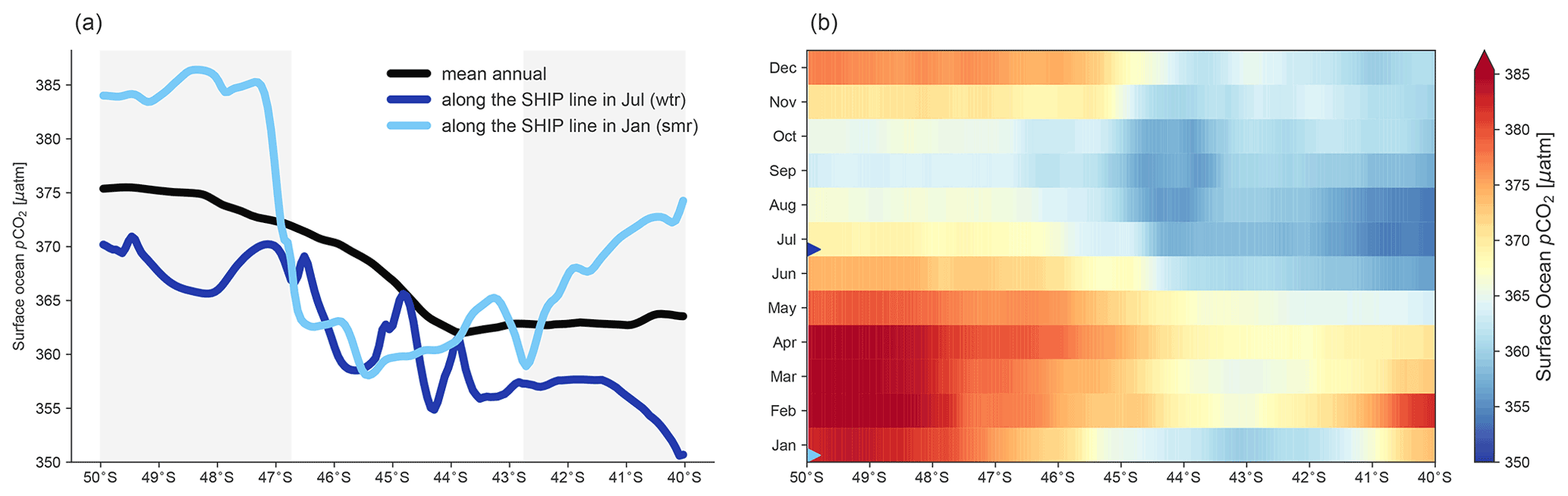
Figure 8 Seasonal contrasts for the meridional gradient (MG) of surface ocean pCO₂ in the experimental sub-domain. Panel (a) shows the mean annual MG (black) and the mean MG along the SHIP line in summer (January) (light blue) and in winter (July) (dark blue); and panel (b) shows the seasonal cycle of the meridional gradient of pCO₂ with the months when the SHIP sampled (blue triangle markers) with the light blue for January (smr) and the dark blue for July (wtr). The light grey shading in panel (a) shows the sub-domain areas (north and south) where there were large differences in pCO₂ meridional gradients along the SHIP line in summer and winter.

Significant differences exist between the meridional gradients along the SHIP line in summer (e.g. January) and winter (e.g. July) (Fig. 8a–b). For example, these differences are more significant farthest south (>47^∘ S) and farthest north (<43^∘ S) compared to the middle (43–47^∘ S) of the sub-domain (light grey shading, Fig. 8a). Similarly, the seasonal cycle difference is not as big in the middle of the sub-domain as it is at the extreme lines of the SAZ and PFZ (Fig. 8b). That is why we need a sampling platform that is able to capture critical scales of variability. Another key point we raised concerning the sampling-scale sensitivity of the pCO₂ reconstructions is that resulting uncertainties and biases depend on the seasonal scale of the meridional gradients of the surface ocean pCO₂ (Fig. 8b). Shedding light on this point results in resolving the seasonal cycle of the meridional gradients.

The similarity of the anomalies between the SHIP(smr) + WG(SAZ) and SHIP(smr) + nUSV experiments is supported by the impact that these sampling strategies have on the seasonal cycle of the bias (Fig. 6b). This shows that, relative to other sampling experiments, there was a reduction in the biases across the whole seasonal cycle but more so in summer–autumn and less so in winter–spring (Fig. 6b). The significantly smaller MBE for SHIP(smr) + WG(SAZ) can be ascribed to the bias being slightly negative in summer–autumn and positive in winter–spring, which leads to a small mean annual MBE, whereas in the case of the SHIP(smr) + WG(PFZ) experiment, the MBE is small but positive throughout (Fig. 6b, and Table 2). The mean annual anomaly map of pCO₂ for the SHIP(smr) + nUSV experiment still shows a positive anomaly, though weaker, at the frontal zone because although the nUSV Saildrone has a daily sampling resolution, it only crosses the highly synoptic SAF zone periodically (Fig. 1c). This is consistent with all the instances when not resolving the temporal variability results in a positive bias of varying magnitudes (Fig. 6b).

On designing an observation-based strategy for quantifying the Southern Ocean uptake of CO₂, Lenton et al. (2006) argued that constraining the net seasonal air–sea CO₂ fluxes within the natural variability in the carbonate system requires doubling the current Southern Ocean meridional sampling. In a semi-idealized experimental setting, our study takes this further by showing that resolving the seasonal cycle of the meridional gradients is very critical. WG and FLOAT provide high temporal sampling resolution, but they do not resolve the existing meridional gradients. Therefore, increasing data density through zonal autonomous sampling vehicles (e.g. floats) is not sufficient to minimize reconstruction errors. The quarterly meridional sampling strategies proposed by Lenton et al. (2006) and Monteiro et al. (2010) could help to resolve the seasonal cycle of the meridional gradients, but they are not operationally feasible.

4.3 Intra-seasonal variability in the seasonal cycle

Recent high-resolution observations using different types of carbon-enabled autonomous platforms have highlighted a potential sensitivity of Southern Ocean CO₂ flux reconstruction uncertainties and mean bias to aliases in sampling the intra-seasonal to seasonal temporal scales (Bushinsky et al., 2019; Gray et al., 2018; Monteiro et al., 2015; Sutton et al., 2021; Williams et al., 2017). Here we discuss the sensitivity of the model domain reconstruction statistical metrics to a range of semi-idealized scenarios of SHIP summer supplemented with FLOAT and WG observations (Table 2; Fig. 6). In each case of FLOAT and WG sampling, they were made to sample each sub-domain (SAZ and PFZ) for a year at their characteristic sampling periods of 10 and 1 d, respectively. The assumption was that the floats would remain in the domain throughout the year. Thus, to not disadvantage the floats in these experiments, one float was deployed in each sub-domain (SAZ and PFZ) as shown in Fig. 1b, under the assumption that floats would not cross the sub-Antarctic front (SAF). The nUSV Saildrone analogue sampling scenario is brought in later to test the predicted sampling requirements to achieve the lowest RMSEs and mean bias error. There was no real benefit in reproducing the zonal sampling approach for the Saildrone (Sutton et al., 2021) because it would be comparable to the zonal travel of FLOAT but with higher daily sampling more akin to the WG. Its metrics would therefore have been comparable to both and would have contributed little to learning.

One of the standout aspects of this part of the analysis, investigating the impact of the sampling period, was the significant difference in the uncertainty and biases between the best-performing SHIP(smr) + WG(SAZ) (RMSE = 6.88; MBE = 0.82 µatm) and SHIP(smr) + FLOAT(PFZ) (RMSE = 8; MBE = 5.32 µatm) scenarios (Table 2). These comparative statistics point to the reconstructions also being very sensitive, particularly to the temporal sampling scales. This finding can be explained and understood from the characteristics of the variability from time series from single model grid cells in the SAZ, on the SAF, and in the PFZ (Fig. 9). Local-scale single-grid-cell observations are appropriate instead of spatial means because they simulate the local nature of the variability and how it is observed. The variability characteristics of these time series help explain the statistics of the pCO₂ reconstructions (Fig. 9; Table 2). The SAZ and SAF are characterized by stronger intra-seasonal variability, whereas the PFZ is characterized by lower-frequency (sub-seasonal)–seasonal modes of variability (Fig. 9). Thus, while the SAZ and SAF sub-domains and their stronger intra-seasonal variability are best resolved by the daily sampling of the WG, the PFZ domain, which is dominated by the lower-frequency sub-seasonal to seasonal cycle, is resolved equally well by the WG daily and FLOAT 10 d sampling periods (Fig. 9; Table 2).

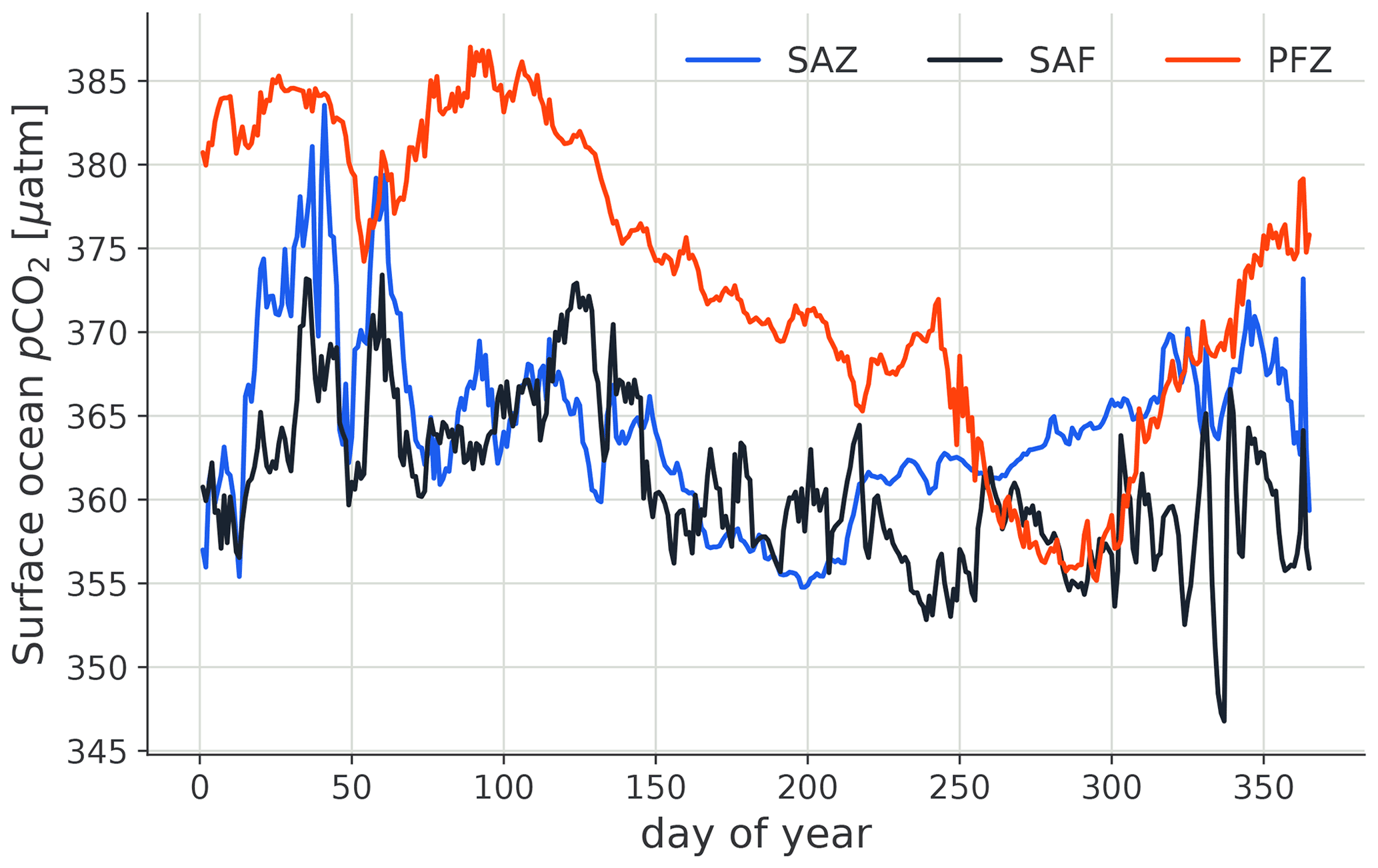
Figure 9 Time series (1 year) plots of the variability in surface ocean pCO₂ at single model grid cells on the SHIP line (2.5^∘ E, Fig. 1b). We used the following single model grid cells: 42^∘ S, 2.5^∘ E in the sub-Antarctic zone (SAZ); 44^∘ S, 2.5^∘ E on the sub-Antarctic front (SAF); and 47^∘ S, 2.5^∘ E in the polar frontal zone (PFZ). The figure shows that while the SAZ and SAF are dominated by synoptic modes of variability, the PFZ is characterized by longer-period sub-seasonal to seasonal scales of variability.

Therefore, given that WG and FLOAT sampling scenarios are comparable in that neither has a strong meridional gradient-resolving sampling strategy, the main difference between them is the daily sampling rate of the WGs and the 10 d sampling rate for FLOAT. Figure 9 then helps explain why even though the domain reconstructions based on the FLOAT(PFZ) sampling scenario perform best out of the two FLOAT scenarios, SHIP(smr) + FLOAT(SAZ + PFZ), ultimately this scenario underperformed relative to the WGs because it was aliasing the synoptic intra-seasonal variability in the SAZ and SAF. This surprising performance of SHIP(smr) + FLOAT(SAZ + PFZ) after running the experiment several times likely resulted from the difference in modes of variability in the SAZ and PFZ (Fig. 9). The float did well when deployed in the PFZ dominated by seasonal variability, which can be resolved by the 10 d sampling period, but performed poorly when it was deployed in the SAZ characterized by intra-seasonal modes, which cannot be resolved by the 10 d sampling period. Thus, when sampling the two sub-domains simultaneously, SHIP(smr) + FLOAT(SAZ + PFZ) resulted in a poorer performance than for the PFZ alone (Fig. 6b; Table 2). The finding that the high temporal resolution of the SHIP(smr) + WG(SAZ) was the only sampling combination to match the performance of the SHIP(smr + wtr) experiment, whose strength was in resolving the seasonal contrasts of the spatial meridional gradient, suggests that these two scales of variability, intra-seasonal and meridional, are close to equally important in achieving a low bias and RMSE reconstruction. Resolving the former and the latter simultaneously may therefore be a presently missing critical step.

More broadly and relative to the SHIP summer-only scenario, all the annual cycle experiments yielded a reduction in the reconstructed seasonal cycle anomalies (Fig. 6b) and in the uncertainties (32 %–50 %) and biases (± 50 %) as well as a statistically significant improvement for Pearson's correlation coefficient (r) (Fig. 6a–b, and Table 2). When comparing SHIP(smr) + WG with SHIP(smr) + FLOAT, reconstructed annual mean pCO₂ maps for the whole domain were consistent with reduced anomalies, for instance, with small positive anomalies for SHIP(smr) + FLOAT(PFZ) and small negative anomalies for SHIP(smr) + WG(SAZ) (Fig. 6d and e, respectively). However, while comparing SHIP(smr) + WG(SAZ) with SHIP(smr) + FLOAT(SAZ) where WGs and floats are both deployed in the SAZ, there is a significant difference in the RMSEs and MBEs with 6.88 and 0.82 µatm, respectively, for the former, and 9.29 and −4.81 µatm, respectively, for the latter (Table 2).

This analysis provides additional understanding of the strengths and limitations of the way that the three main autonomous platforms (Wave Gliders, carbon floats, and Saildrones) deployed in the Southern Ocean contribute to increasing or decreasing the seasonal cycle and mean annual biases as well as the RMSEs (Monteiro et al., 2015; Bushinsky et al., 2019; Sutton et al., 2021). Based on hourly observations of the surface ocean pCO₂, Monteiro et al. (2015) showed that a temporal sampling resolution of less than 2 d would be necessary in 30 %–40 % of the Southern Ocean, corresponding to the SAZ, to reduce the uncertainty to less than 10 % of the annual mean (Sect. S3.5). Our study confirms the sensitivity of the RMSE of the intra-seasonal variability sampling alias and also shows its impacts on the bias of the annual mean. SOCCOM-float-calculated pCO₂ data have made a decisive impact on resolving the seasonal cycle in the Southern Ocean and suggest that winter CO₂ outgassing may be underestimated in SOCAT-based reconstructions (Bushinsky et al., 2019; Gray et al., 2018). Our study suggests that these observed and reconstructed elevated outgassing fluxes may be the result of both aliasing of the intra-seasonal variability and not resolving the seasonal cycle of the meridional gradient. Our analysis also raises a question about the assumption that not resolving the intra-seasonal variability in pCO₂ does not contribute significantly to the RMSE and the bias (Bushinsky et al., 2019). It shows that the intra-seasonal modes of the wind are not sufficient to impart a low mean annual and seasonal cycle bias.

To provide a more quantitative characterization of our findings, an additional analysis was conducted on the sub-10 d mode of variability. A 10 d rolling mean was used to eliminate or weaken the sub-10 d mode of variability (Fig. S8a). The difference between this 10 d rolling mean and the daily model output gives the high-frequency variability, and the root mean square error (RMSE) gives us a statistical understanding of what the uncertainty might be if we sampled at a 10 d rate (shown in Fig. S8b as a map). The resulting mean RMSEs for the SAZ and PFZ, after implementing the 10 d rolling mean, are 2.53 and 1.71 µatm, respectively, a significant reduction relative to the RMSEs for the FLOAT experiment using the daily model output (Table 2). This provides further quantitative support for our findings and the work of Monteiro et al. (2015) that more dynamic regions require higher sampling rates. We finally propose that the impact of SOCCOM floats on the reconstructions can be strengthened by reducing the sampling period to <2 d, especially in high-EKE areas and through a coordinated meridional deployment strategy that helps to resolve the meridional gradient across the annual cycle. Our study also suggests that notwithstanding the high temporal frequency of the USV Saildrone, the present emphasis on a zonal sampling pattern (Sutton et al., 2021) also underestimates the potential contribution that this platform could make in observing the seasonal cycle of the meridional gradient at high temporal resolution simultaneously. We now examine this aspect in more detail.

4.4 Getting over the wall in the Southern Ocean by simultaneously resolving the intra-seasonal and seasonal variability in the meridional gradient – proposed optimal sampling strategy

This analysis has highlighted that in order to minimize the uncertainties and biases sufficiently to get over the wall, observational strategies in the Southern Ocean need to simultaneously resolve the seasonal cycle of the meridional gradient at temporal scales that also resolve, where necessary, the intra-seasonal variability. To test this hypothesis, we designed an additional year-round observing system simulation experiment (OSSE) that simulated the spatial and temporal sampling capabilities of the new unmanned surface vehicle (nUSV) Saildrone (Sutton et al., 2021) to supplement the SHIP summer-only sampling SHIP(smr) (Figs. 1c and 6 and h), that is, SHIP(smr) + nUSV. This experiment combined the speed of the nUSV Saildrone (Gentemann et al., 2020; Meinig et al., 2019) required to cover the regional meridional spatial gradient length scales (Fig. 1c) with high-frequency daily sampling to supplement SHIP(smr). Together these fulfil the requirements that emerged from the earlier analysis.

Comparative statistics show that the SHIP(smr) + nUSV experiment yielded a very significant improvement in the reconstruction skills relative to all other platform combinations (Table 2). Its performance metrics (RMSE = 6.4 µatm) outperformed the next best combination SHIP(smr) + WG(SAZ) (RMSE = 6.88 µatm) and SHIP(smr) + FLOAT(PFZ) (RMSE = 8.0 µatm). This supports the hypothesis that resolving the intra-seasonal and seasonal variabilities in the meridional gradients is decisive in minimizing uncertainties and bias in pCO₂ reconstructions. Based on this analysis, we propose that the optimal sampling scheme is SHIP + nUSV because it not only provides a high temporal resolution (daily) of the large-scale meridional gradients but also combines speed to cover the required meridional spatial extent.

The nUSV Saildrones are still relatively new autonomous sampling platforms, and their ability to withstand the stringent weather and sea conditions in the Southern Ocean is still being assessed (Sutton et al., 2021). Recent deployments of Saildrones have been focused on zonal circumpolar tracks, which have been successful in proving the Saildrones as a robust sampling platform and in observing the seasonal cycle of CO₂ fluxes in the sub-polar domain (Sutton et al., 2021). This approach is comparable to the zonal sampling of FLOAT (Fig. 1b) but with a higher temporal sampling frequency (daily vs. 10 d). Notwithstanding the higher temporal sampling frequency from the Saildrone, the lack of a meridional spatial component to the zonal sampling strategy limits its value in reducing the uncertainties and biases in any reconstructions that use them. Its inclusion in CO₂ flux reconstructions would improve the RMSE and mean bias error (MBE) relative to SOCAT-based reconstructions, which, as discussed earlier, are not where autonomous sampling vehicles can add the best value (Tables 1 and 2).

Our work here shows that a zonal sampling strategy, while good for operational navigational reasons, is not the most efficient way to maximize the value of USV Saildrone sampling to resolve critical scales of variability necessary for high confidence in the pCO₂ and inferred CO₂ flux reconstructions in the Southern Ocean. Furthermore, our study shows how, by mixing the meridional sampling strategy (Lenton et al., 2006; Monteiro et al., 2010) with the current zonal sampling, we can leverage the USV Saildrones to make sure we are not missing the meridional gradients.

4.5 Applicability of the sub-domain to the wider Southern Ocean

The focus of this study was on investigating the mismatch between sampling periods and the modes of variability in pCO₂ in the domain rather than the mechanisms. This selected domain in the south-east (SE) Atlantic Ocean encapsulates the contrasts in the scales of variability of interest, namely the seasonal and intra-seasonal modes that are characteristic of the Southern Ocean (Fig. 10). It shows how findings in the study domain can be extended to the Southern Ocean. Using a 10-year period of pCO₂ output from NEMO-PISCES model simulations at a 5 d temporal mean, the seasonal cycle reproducibility (SCR) of pCO₂ was calculated as the correlation of the detrended pCO₂ with its own 10-year climatology – the larger the correlation, the stronger the SCR (Thomalla et al., 2011). This resulted in the SCR-based clustering of the Southern Ocean into three regions (Fig. 10) corresponding to the low-SCR (LSCR), medium-SCR (MSCR), and high-SCR (HSCR) areas, respectively. The criteria of the choice of these three ranges are as follows. In high-SCR areas, there is no intra-seasonal variability and there are no annual signals. In medium-SCR areas, intra-seasonal variability emerges but is smaller in magnitude compared to the seasonal cycle, while in low-SCR areas, there is no seasonal signal and the intra-seasonal variability is larger than the seasonal cycle.

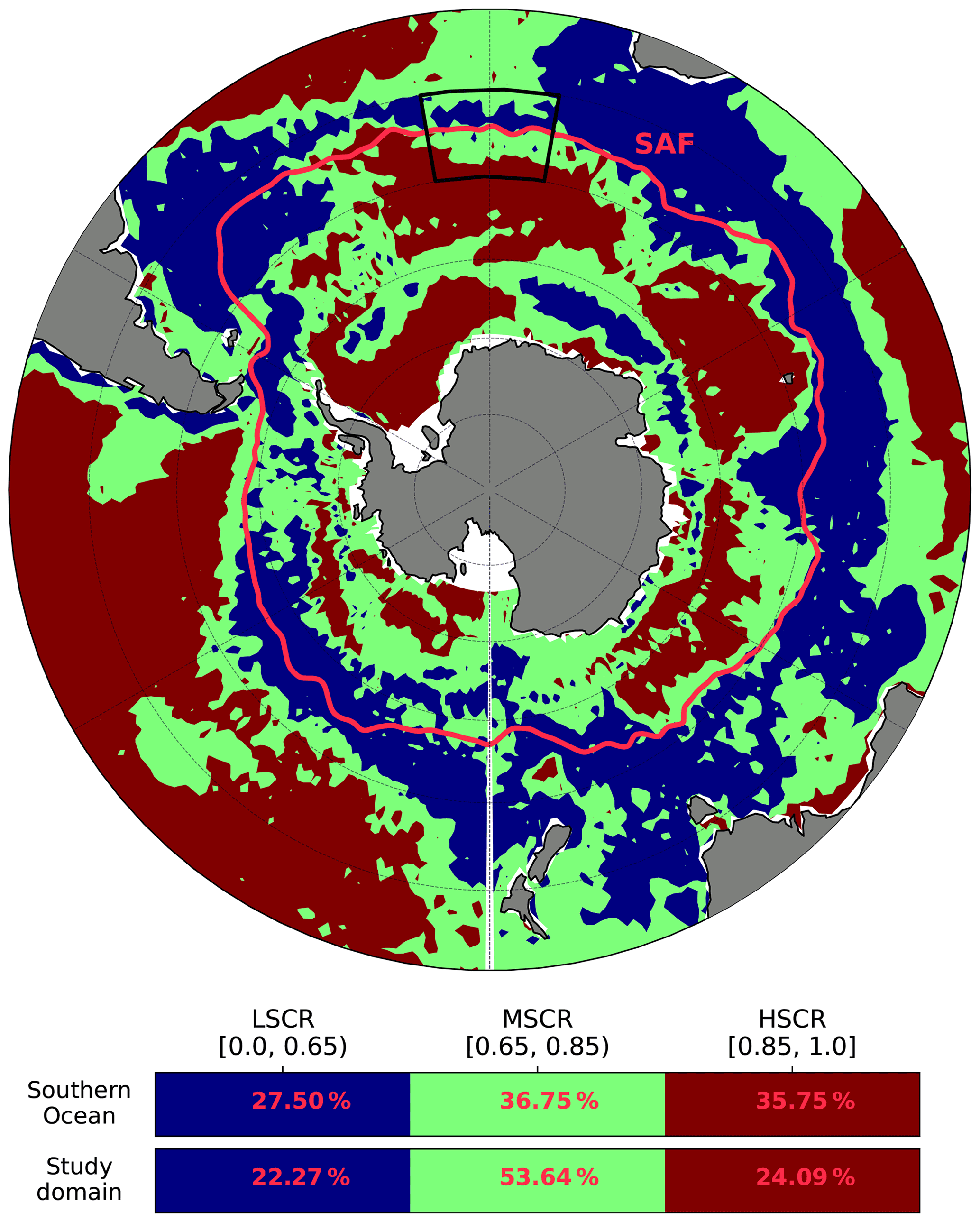
Figure 10 Map showing the study domain and the Southern Ocean sub-regions resulting from the seasonal cycle reproducibility (SCR) of pCO₂ calculated based on 10 years of NEMO-PISCES simulations at the 5 d temporal resolution, where the sub-Antarctic front (SAF) (light red) and the study domain (black box) are depicted. The table below the map shows the fraction coverage estimates (%) for these SCR-based regions both in the domain and in the Southern Ocean as a whole. LSCR corresponds to low-SCR areas, while MSCR and HSCR represent medium- and high-SCR areas, respectively.

Although this study domain was chosen within a high-EKE area (black box; Figs. 1a, 10) because of its contrasting seasonal and intra-seasonal variability in the surface ocean pCO₂, the SCR metric shows how the study area in the SE Atlantic Ocean contrasts the Southern Ocean as a whole (Fig. 10). As argued in the previous paragraph, seasonal and intra-seasonal variability is relatively associated with LSCR (0–0.65) and MSCR (0.65–0.85) regions, which together represent ∼ 75 % of the study domain and ∼ 64 % of the whole Southern Ocean (cf. Table shown in Fig. 10). This demonstrates that the sub-domain modes of variability (which are dominantly intra-seasonal) may be applied to the wider Southern Ocean.

Longitudinally, the Southern Ocean is equal to $\mathrm{360}{}^{\circ }/\mathrm{20}{}^{\circ }$ = 18 times our 20^∘ W–E domain. However, while in theory, our domain is $\mathrm{1}/\mathrm{18}$th of the zonal extent of the Southern Ocean, it represents different modes of variability as argued above. Thus, we should be able to capture the variability with fewer than 18 USV Saildrones. Based on this, we have a speculative estimate of the monetary cost; see the Supplement (Sect. S3.4). A study on the full Southern Ocean will be performed to assess this more thoroughly.

4.6 Limitations of the study

In this study, our limitations were tied to four main points: the model used, the selected sub-domain, the existing shift in the seasonal cycle phasing of the model and data products, and the overfitting tendency of ML models. Here we discuss these limitations separately.

We only had 1 year of daily outputs of the high-resolution coupled (NEMO-PISCES) ocean model, BIOPERIANT12 (BP12). These BP12 model spatial ($\mathrm{1}/\mathrm{12}{}^{\circ }$ by $\mathrm{1}/\mathrm{12}{}^{\circ }$) and temporal (daily) resolutions influenced the designing of the OSSEs, therefore impacting the sampling approach of the synthetic platforms compared to their real-world counterparts. For example, unlike other sampling platforms that can be driven remotely, floats are harder to simulate due to the way they operate. Thus, we could only mimic the 10 d sampling period and the deployment location and assume that they are randomly transported eastwards by the water current. Since the Antarctic Circumpolar Current (ACC) moves eastwards, the random walk we implemented is an adequate approximation and adds an element of stochasticity that is likely close to reality (Fig. 1b).

The selected sub-domain combines regional and mesoscale gradients and features (such as eddies and fronts) which could challenge the reconstruction methods to better capture some variability scales such as the seasonal cycle of the meridional gradients (Fig. 8). However, the meridional gradients could also be associated with the meandering of the ACC fronts such as the SAF, which crosses the domain. On the other hand, the assumption of the domain representativeness of the variability scales of the region could be a cause for concern as this would be applicable in regions where latitudinal gradients are strong. For example, the BP12 model output might not achieve this assumption based on a standard deviation of 9.1 µatm for the synthetic SHIP data compared to 20.96 µatm for SOCAT data in the sub-domain.

Existing differences in the mean pCO₂ seasonal cycles of the model and data products (Fig. 2) could also result from processes that deterministic models such as the BP12 ocean model (NEMO-PISCES) cannot yet constrain due to a lack of understanding of the complete Southern Ocean carbonate system or mixed-layer physics (Lenton et al., 2013; Mongwe et al., 2016; Monteiro et al., 2015). However, our knowledge of which one is right between model and data products remains limited.

Lastly, overfitting is a common challenge in supervised machine learning (ML) problems. Although each of the two ML algorithm (FNN and GBM; see Sect. 2.4) best practices were used in training, the GBM algorithm encountered more challenges with the overfitting compared to the FNN (cf. Table S3). While GBM has been proven to deal well with imbalanced or sparse datasets (Ke et al., 2017), it is more likely to overfit the training data because of the model's potential for high complexity (Frery et al., 2017).

Finally, while studies such as Gregor et al. (2019), Devil-Sommer et al. (2019), and Gloege et al. (2021) found that mixed-layer depth (MLD) climatology is an important predictor of surface ocean pCO₂, our use of dynamic model-generated MLD may impart some advantage that might not be available to the real-world observation-based reconstructions. Moreover, we also recognize that model-generated Chl a may not be, in absolute terms, directly analogous to satellite Chl a. However, these advantages from using model output are uniform across all the sampling experiments in this study.

5 Conclusions

From this study, we propose that one can advance the uncertainties and biases from machine learning pCO₂ reconstructions beyond the wall, at least in the Southern Ocean. Within a chosen experimental domain of the Southern Ocean, we demonstrate that this would require resolving the seasonal and intra-seasonal modes of variability in the meridional gradients of pCO₂ through a combination of high-frequency (at least daily) observations spanning the meridional axis. We showed that the reconstructed seasonal cycle anomaly and mean annual pCO₂ are highly sensitive to seasonal sampling biases. The seasonal sampling bias comprises both the temporal and the meridional spatial scales of variability. This may explain the significant winter-positive bias in the reconstruction of the seasonal cycle of pCO₂ in the domain, which likely may also contribute to the apparent winter-maximum outgassing or weakening of the ingassing of CO₂ observed in recent Southern Ocean data products. This points to an urgent need to address the existing seasonal bias (towards summer) in the Southern Ocean SOCAT dataset through improving the sampling strategy of the present autonomous platforms so that they are better aligned to the integrated spatial and temporal sampling-scale needs.

Inside the chosen domain, the study confirmed that not resolving the high-frequency (synoptic–sub-seasonal) variability results in insufficient decreases in mean biases and RMSE scores for the reconstructed mean annual flux. Present 10 d sampling periods of floats have a limited impact on reducing uncertainties and biases in pCO₂ mappings because they do not resolve the intra-seasonal variability. In addition, the predominantly zonal and quasi-Lagrangian sampling does not contribute sufficiently to resolving the seasonal variability in the meridional gradients of pCO₂. Our study proposes that a more meridionally coordinated deployment of floats could contribute further to resolving synoptic variability and the meridional gradients. For example, increasing sampling frequency to <2 d, particularly in high-EKE areas, as well as a meridionally coherent sampling strategy would support resolving the synoptic-scale variability and the variability in the basin-scale gradients. Although they still lack the meridional gradient reach, Wave Gliders in pseudo-mooring modes improve on floats (RMSEs, MBEs), and the main explanation for this improvement is because of their higher sampling frequency (daily). This study recommends that the use of Wave Gliders in the reconstruction of CO₂ fluxes in the pseudo-mooring mode should be discontinued and a meridional dimension to the high temporal resolution (1–2 d) should be adopted. We showed that while the USV Saildrones in the present zonal sampling mode improve the RMSEs and biases, this might not be the most efficient way to maximize their strengths stemming from their high sampling frequency (hourly) and large spatial scale (by leveraging their speed). We thus propose that USV Saildrones are probably the optimal platforms to address the necessary integrated large-scale spatial and high-resolution temporal sampling.

In summary, ship-based observations (SOCAT-like) remain vital to the reconstruction of CO₂ fluxes in the Southern Ocean as a whole and should be continued. These observations are the baseline data involved in the training of any machine learning algorithms behind the main observation-based products of reference. However, these ship-based observations are seasonally biased (towards summer) due to under-sampling during stormy autumn and winter seasons, which is likely the root of persistently elevated uncertainties and a winter-positive bias in the reconstructions. This bias should be addressed with urgency. Finally, this study proposes that a meridional sampling strategy may be an efficient way of sampling using autonomous observing systems. In this case, we recommend that existing ship-based observations of the surface ocean pCO₂ in the Southern Ocean should be supplemented by year-round autonomous high-resolution observations that resolve the seasonal cycle of the meridional gradients of the surface ocean pCO₂. However, a follow-up study is also recommended to test, for example, the USV Saildrone effectiveness and impact on reducing uncertainties and biases in the seasonal and mean annual reconstruction of CO₂ fluxes in the Southern Ocean as a whole.