Impact of negative and positive CO₂ emissions on global warming metrics using an ensemble of Earth system model simulations

The benefits of implementing negative emission technologies in the global warming response to cumulative carbon emissions until the year 2420 are assessed following the shared socioeconomic pathway (SSP) 1-2.6, the sustainable development scenario, with a comprehensive set of intermediate-complexity Earth system model integrations. Model integrations include 86 different model realisations covering a wide range of plausible climate states. The global warming response is assessed in terms of two key climate metrics: the effective transient climate response to cumulative CO₂ emissions (eTCRE), measuring the surface warming response to cumulative carbon emissions and associated non-CO₂ forcing, and the effective zero emissions commitment (eZEC), measuring the extent of any continued warming after net-zero CO₂ emissions are reached. The transient climate response to cumulative CO₂ emissions (TCRE) is estimated as 2.2 K EgC⁻¹ (median value) with a 10 %–90 % range of 1.75 to 3.13 K EgC⁻¹ in 2100, approximated from the eTCRE by removing the contribution of non-CO₂ forcing. During the positive emission phase, the eTCRE decreases from 2.71 (2.0 to 3.65) to 2.61 (1.91 to 3.62) K EgC⁻¹ due to a weakening in the dependence of radiative forcing on atmospheric carbon, which is partly opposed by an increasing fraction of the radiative forcing warming the surface as the ocean stratifies. During the net negative and zero emission phases, a progressive reduction in the eTCRE to 2.0 (1.39 to 2.96) K EgC⁻¹ is driven by the reducing airborne fraction as atmospheric CO₂ is drawn down mainly by the ocean. The model uncertainty in the slopes of warming versus cumulative CO₂ emissions varies from being controlled by the radiative feedback parameter during positive emissions to being affected by carbon-cycle parameters during net negative emissions, consistent with the drivers of uncertainty diagnosed from the coefficient of variation of the contributions in the eTCRE framework. The continued warming after CO₂ emissions cease and remain at zero gives a model mean eZEC of −0.03 K after 25 years, which decreases in time to −0.21 K at 90 years after emissions cease. However, there is a spread in the ensemble with a temperature overshoot occurring in 20 % of the ensemble members at 25 years after cessation of emissions. If net negative emissions are included, there is a reduction in atmospheric CO₂ and there is a decrease in temperature overshoot so that the eZEC is positive in only 5 % of the ensemble members. Hence, incorporating negative emissions enhances the ability to meet climate targets and avoid risk of continued warming after net zero is reached.

1 Introduction

There is an increasing need to adopt negative emission technologies (Luderer et al., 2013; Rogelj et al., 2015; Beerling et al., 2020) to enhance the chance of meeting the Paris climate agreement target (UNFCCC, 2015) to hold global warming well below 2 ^∘C with an ambition of 1.5 ^∘C given the ongoing growth in greenhouse gas concentrations (Boucher et al., 2012; Jeltsch-Thömmes et al., 2020). For a 1.5 ^∘C target, there is a 66 % chance of meeting this target only if post-2019 cumulative carbon emissions are limited to less than ∼ 400 GtCO₂ (IPCC, 2021). Two climate metrics of transient climate response to cumulative CO₂ emissions (TCRE) and zero emissions commitment (ZEC) are essential to determine how much carbon may be emitted while remaining within the warming target.

The remaining carbon budget is inversely proportional to the TCRE, the increase in the global mean surface air temperature relative to cumulative CO₂ emissions (Matthews et al., 2009; Zickfeld et al., 2012; IPCC, 2013; Gillett et al., 2013; Zickfeld et al., 2013; Friedlingstein et al., 2014; Matthews et al., 2017). Climate model projections reveal a simple near-linear relationship between the global surface air temperature change and cumulative CO₂ emissions between 0 and ∼ 2000 PgC (MacDougall, 2016). However, despite a similar linear dependence, there is a wide inter-model range in TCRE values (Williams et al., 2017a; Spafford and MacDougall, 2020), varying from 1.4 to 2.5 K EgC⁻¹ in intermediate-complexity Earth system models (Eby et al., 2013), 0.8 to 2.4 K EgC⁻¹ in full-complexity Earth system models (Matthews et al., 2018) and 0.7 to 2.0 K EgC⁻¹ (90 % confidence interval) in observationally constrained TCRE estimates from a 15-member Coupled Model Intercomparison Project (CMIP) 5 ensemble (Gillett et al., 2013).

For the case of radiative forcing exclusively from atmospheric CO₂, the TCRE can be related to the dependence of the global mean temperature on the radiative forcing, the dependence of the radiative forcing on the atmospheric CO₂ and the airborne fraction (Sect. 2; Williams et al., 2016; Ehlert et al., 2017; Katavouta et al., 2018; Williams et al., 2020). Applying this framework to seven CMIP5 and nine CMIP6 models following a 1 % annual increase in atmospheric CO₂, the TCRE is affected by a large inter-model spread in the climate feedback parameter for CMIP6 (Williams et al., 2020) as well as by a larger inter-model spread in the land carbon system for CMIP5 (Jones and Friedlingstein, 2020). The inclusion of non-CO₂ radiative forcing alters the relationship between emissions and surface warming through both direct warming and carbon feedback effects (Tokarska et al., 2018). For the more realistic case including non-CO₂ radiative-forcing contributions, the TCRE may be estimated by approximately removing the warming linked to non-CO₂ radiative forcing (Matthews et al., 2021). Alternatively, an effective TCRE (eTCRE) may be defined to include non-CO₂ warming and the non-CO₂ radiative forcing (Williams et al., 2016, 2017a).

The climate response after net-zero emissions is an important climate metric, encapsulated in the zero emissions commitment (ZEC) given by the mean surface air temperature change after CO₂ emissions cease (Hare and Meinshausen, 2006; Matthews and Caldeira, 2008; Froelicher and Paynter, 2015; MacDougall et al., 2020). Quantification of the ZEC is critical for calculating the remaining carbon budget. Whether there is continued surface warming depends on competition between a cooling effect from the reduction in the radiative forcing from atmospheric CO₂ as carbon is taken up by the ocean and terrestrial biosphere and a surface warming effect from a decline in the heat uptake by the ocean interior (Williams et al., 2017b). In an analysis of Earth system model responses to idealised CO₂-only forcing, MacDougall et al. (2020) found a multi-model mean ZEC close to zero, with a wide spread in continued warming and cooling responses from individual models. Matthews and Zickfeld (2012) previously analysed the ZEC in the context of a realistic scenario by including contributions from non-CO₂ forcings, but these authors did not address uncertainty. We address this gap by applying a perturbed physics ensemble to an experiment which includes non-CO₂ forcing within the framework of a strong-mitigation scenario as is most appropriate for negative emissions.

Here we examine these two climate metrics, the TCRE and the ZEC, following the shared socioeconomic pathway (SSP) 1-2.6 scenario, which combines realistic socioeconomic conditions for sustainable development with the high-mitigation Representative Concentration Pathway (RCP) 2.6 scenario assuming large-scale employment of a range of greenhouse gas mitigation technologies and strategies. Our analysis is based on simulations with the intermediate-complexity Earth system model, Grid-ENabled Integrated Earth system model (GENIE-1). The use of intermediate complexity enables us to (i) quantify uncertainties through an ensemble consisting of 86 members that provide a wide range of plausible climate states and (ii) explore long timescales, in both historical and future periods. The pre-industrial baseline is chosen as 850 CE (Eby et al., 2013) rather than 1850 CE to account for both land use change and fossil fuel CO₂ emissions occurring before 1850 CE. The reconstructions of land use change emissions for the periods prior to about 1800 have been based on prior estimates of population, mortality rate and land use assumptions and hold large uncertainties (Koch et al., 2019). The model was spun up to a pre-industrial climate and integrated from years 850 to 2420 CE, extending several centuries after the emissions cease to reveal whether there is continued warming and to quantify the effectiveness of negative emission applications. The TCRE analysis follows an eTCRE framework (Williams et al., 2016; Ehlert et al., 2017; Katavouta et al., 2018; Williams et al., 2020) and is compared with a correlation analysis between the varied model parameters and the slopes of change in temperature versus cumulative emissions. The effective ZEC (eZEC) analysis addresses the response of the ensemble during periods of net-zero carbon emissions but continued non-CO₂ forcing following the SSP1-2.6 scenario.

In this study, the theoretical framework used to interpret the TCRE is set out including defining its thermal, radiative and carbon contributions (Sect. 2). The model methodology using the intermediate-complexity Earth system model GENIE-1 (Sect. 3) and the model responses including the spread in ensemble responses (Sect. 4) are described. The controls of the climate responses as defined by the two climate metrics, the effective TCRE and effective ZEC, are explored, including outlining the asymmetrical response to positive and negative emissions (Sect. 5). Finally, the implications of the study are summarised, including the benefits of implementing negative emissions (Sect. 6).

2 Theoretical framework

We first introduce the framework under the assumption of only CO₂ forcing. A climate metric TCRE (in K EgC⁻¹) is defined as the surface warming response to cumulative CO₂ emissions:

$$\begin{array}{}\text{(1)}& \mathrm{TCRE}={\displaystyle \frac{\mathrm{\Delta }T\left(t\right)}{I_{\mathrm{em}}\left(t\right)}},\end{array}$$

where Δ is the change since year 850 CE, ΔT(t) is the global mean change in surface air temperature (in K), and I_em(t) is the cumulative CO₂ emissions (in PgC) from the sum of fossil fuel emissions and land use changes.

The TCRE may be viewed as a product of two terms, the change in global mean air temperature divided by the change in the atmospheric carbon inventory, $\mathrm{\Delta }T\left(t\right)/\mathrm{\Delta }{I}_{\mathrm{atmos}}\left(t\right)$, and the airborne fraction, $\mathrm{\Delta }{I}_{\mathrm{atmos}}\left(t\right)/I_{\mathrm{em}}\left(t\right)$, given by the change in the atmospheric carbon inventory (in PgC) divided by the cumulative CO₂ emissions (Matthews et al., 2009; Solomon et al., 2009; Gillett et al., 2013; MacDougall, 2016), such that

$$\begin{array}{}\text{(2)}& \mathrm{TCRE}\equiv {\displaystyle \frac{\mathrm{\Delta }T\left(t\right)}{I_{\mathrm{em}}\left(t\right)}}=\left({\displaystyle \frac{\mathrm{\Delta }T\left(t\right)}{\mathrm{\Delta }{I}_{\mathrm{atmos}}\left(t\right)}}\right)\left({\displaystyle \frac{\mathrm{\Delta }{I}_{\mathrm{atmos}}\left(t\right)}{I_{\mathrm{em}}\left(t\right)}}\right),\end{array}$$

where $\mathrm{\Delta }T\left(t\right)/\mathrm{\Delta }{I}_{\mathrm{atmos}}\left(t\right)$ is related to the transient climate response, defined by the temperature change at the time of doubling of atmospheric CO₂ (Matthews et al., 2009). The TCRE is defined in terms of this surface warming response to CO₂ forcing, usually following a 1 % annual rise in atmospheric CO₂.

Alternatively, the TCRE may be linked to an identity involving a thermal dependence on radiative forcing, defined by the change in temperature divided by the change in radiative forcing, ΔF(t) (in W m⁻²), and the radiative-forcing dependence on CO₂ emissions, defined by the change in radiative forcing divided by the cumulative CO₂ emissions (Goodwin et al., 2015; Williams et al., 2016, 2017a), such that

$$\begin{array}{}\text{(3)}& \mathrm{TCRE}\equiv {\displaystyle \frac{\mathrm{\Delta }T\left(t\right)}{I_{\mathrm{em}}\left(t\right)}}=\left({\displaystyle \frac{\mathrm{\Delta }T\left(t\right)}{\mathrm{\Delta }F\left(t\right)}}\right)\left({\displaystyle \frac{\mathrm{\Delta }F\left(t\right)}{I_{\mathrm{em}}\left(t\right)}}\right).\end{array}$$

These two viewpoints can be rationalised by rewriting the radiative-forcing dependence on CO₂ emissions in Eq. (3) in terms of the radiative-forcing dependence on atmospheric CO₂ and the airborne fraction (Ehlert et al., 2017; Katavouta et al., 2018; Williams et al., 2020).

The TCRE is then defined by the product of the thermal dependence, the radiative dependence between radiative forcing and atmospheric carbon, and the carbon dependence involving the airborne fraction:

$$\begin{array}{}\text{(4)}& \mathrm{TCRE}\equiv {\displaystyle \frac{\mathrm{\Delta }T\left(t\right)}{I_{\mathrm{em}}\left(t\right)}}=\underset{\mathrm{thermal}}{\underbrace{\left({\displaystyle \frac{\mathrm{\Delta }T\left(t\right)}{\mathrm{\Delta }F\left(t\right)}}\right)}}\underset{\mathrm{radiative}}{\underbrace{\left({\displaystyle \frac{\mathrm{\Delta }F\left(t\right)}{\mathrm{\Delta }{I}_{\mathrm{atmos}}\left(t\right)}}\right)}}\underset{\mathrm{carbon}}{\underbrace{\left({\displaystyle \frac{\mathrm{\Delta }{I}_{\mathrm{atmos}}\left(t\right)}{\mathrm{\Delta }{I}_{\mathrm{em}}\left(t\right)}}\right)}}.\end{array}$$

The thermal response may be further understood from an empirical global radiative balance (Gregory et al., 2004; Forster et al., 2013). The increase in radiative forcing, ΔF(t), drives an increase in planetary heat uptake, N(t) (in W m⁻²), plus a radiative response, which is assumed to be equivalent to the product of the increase in global mean surface air temperature, ΔT(t), and the climate feedback parameter, λ(t) (in W m⁻² K⁻¹):

$$\begin{array}{}\text{(5)}& \underset{\mathrm{radiative}\mathrm{forcing}}{\underbrace{\mathrm{\Delta }F\left(t\right)}}=\underset{\mathrm{heat}\mathrm{uptake}}{\underbrace{N\left(t\right)}}+\underset{\mathrm{radiative}\mathrm{response}}{\underbrace{\mathit{\lambda }\left(t\right)\mathrm{\Delta }T\left(t\right)}}.\end{array}$$

The thermal dependence in Eq. (4) given by the dependence of surface warming on radiative forcing, $\mathrm{\Delta }T\left(t\right)/\mathrm{\Delta }F\left(t\right)$, is then given by the product of the inverse of the climate feedback, λ⁻¹(t), and the planetary heat uptake divided by the radiative forcing, $N\left(t\right)/\mathrm{\Delta }F\left(t\right)$:

$$\begin{array}{}\text{(6)}& {\displaystyle \frac{\mathrm{\Delta }T\left(t\right)}{\mathrm{\Delta }F\left(t\right)}}={\displaystyle \frac{\mathrm{1}}{\mathit{\lambda }\left(t\right)}}\left(\mathrm{1}-{\displaystyle \frac{N\left(t\right)}{\mathrm{\Delta }F\left(t\right)}}\right),\end{array}$$

where $\mathrm{1}-N\left(t\right)/\mathrm{\Delta }F\left(t\right)$ represents the fraction of the radiative forcing that is lost to space and may be viewed as effectively equivalent to the fraction of the radiative forcing that warms the surface rather than the ocean interior.

The carbon dependence in Eq. (4) involving the airborne fraction, $\mathrm{\Delta }{I}_{\mathrm{atmos}}\left(t\right)/I_{\mathrm{em}}\left(t\right)$, is related to the changes in the ocean-borne, land-borne and sediment-borne fractions (Jones et al., 2013):

$$\begin{array}{}\text{(7)}& {\displaystyle \frac{\mathrm{\Delta }{I}_{\mathrm{atmos}}\left(t\right)}{I_{\mathrm{em}}\left(t\right)}}=\mathrm{1}-\left({\displaystyle \frac{\mathrm{\Delta }{I}_{\mathrm{ocean}}\left(t\right)}{I_{\mathrm{em}}\left(t\right)}}+{\displaystyle \frac{\mathrm{\Delta }{I}_{\mathrm{land}}\left(t\right)}{I_{\mathrm{em}}\left(t\right)}}+{\displaystyle \frac{\mathrm{\Delta }{I}_{\mathrm{sediment}}\left(t\right)}{I_{\mathrm{em}}\left(t\right)}}\right),\end{array}$$

where the changes in the ocean, land and sediment inventories are denoted by ΔI_ocean(t), ΔI_land(t) and ΔI_sediment(t) (in PgC), respectively.

The TCRE is formally defined in terms of the climate response to cumulative CO₂ emissions following a 1 % annual rise in atmospheric CO₂ (Matthews et al., 2009). As the rise in anthropogenic radiative forcing is currently dominated by the radiative forcing from atmospheric CO₂, the TCRE is a useful climate metric to understand future climate projections. However, in the more realistic framework we apply here, the warming response includes contributions from non-CO₂ forcing. In such experiments, Matthews et al. (2021) advocate estimating the TCRE by approximately removing the warming due to the non-CO₂ radiative forcing by multiplying by a non-dimensional factor (1−f_nc), now explicitly acknowledging that ΔT(t) is not solely driven by I_em(t):

$$\begin{array}{}\text{(8)}& \mathrm{TCRE}={\displaystyle \frac{\mathrm{\Delta }T\left(t\right)}{I_{\mathrm{em}}\left(t\right)}}\left(\mathrm{1}-f_{\mathrm{nc}}\right).\end{array}$$

Matthews et al. (2021) interpret the non-dimensional factor (1−f_nc) as representing the non-CO₂ fraction of total anthropogenic forcing where $f_{\mathrm{nc}}=(\mathrm{\Delta }F\left(t\right)-\mathrm{\Delta }{F}_{{\mathrm{CO}}_{\mathrm{2}}}\left(t\right))/\mathrm{\Delta }F\left(t\right)$. This estimation of the TCRE from general forcing scenarios assumes that the time – and scenario – independence of the TCRE translates to a general response independence from radiative-forcing elements.

In order to allow for possible changes in the thermal and carbon responses from the non-CO₂ forcing, we prefer to define an eTCRE including the effect of the radiative forcing from non-CO₂ and CO₂ radiative components using a series of mathematical identities (Williams et al., 2016, 2017a), where

$$\begin{array}{}\text{(9)}& \begin{array}{rl}& \mathrm{eTCRE}\equiv {\displaystyle \frac{\mathrm{\Delta }T\left(t\right)}{I_{\mathrm{em}}\left(t\right)}}=\\ & \underset{\mathrm{thermal}}{\underbrace{\left({\displaystyle \frac{\mathrm{\Delta }T\left(t\right)}{\mathrm{\Delta }F\left(t\right)}}\right)}}\underset{\mathrm{radiative}\mathrm{from}{\mathrm{CO}}_{\mathrm{2}}\mathrm{and}\text{non-}{\mathrm{CO}}_{\mathrm{2}}}{\underbrace{\left({\displaystyle \frac{\mathrm{\Delta }F\left(t\right)}{\mathrm{\Delta }{F}_{{\mathrm{CO}}_{\mathrm{2}}}\left(t\right)}}\right)\left({\displaystyle \frac{\mathrm{\Delta }{F}_{{\mathrm{CO}}_{\mathrm{2}}}\left(t\right)}{\mathrm{\Delta }{I}_{\mathrm{atmos}}\left(t\right)}}\right)}}\underset{\mathrm{carbon}}{\underbrace{\left({\displaystyle \frac{\mathrm{\Delta }{I}_{\mathrm{atmos}}\left(t\right)}{\mathrm{\Delta }{I}_{\mathrm{em}}\left(t\right)}}\right)}}.\end{array}\end{array}$$

By including the effect of the non-CO₂ radiative forcing, the eTCRE in Eq. (9) is larger than the TCRE with non-CO₂ radiative forcing removed in Eq. (8) whenever the positive radiative effect of non-CO₂ greenhouse gases exceeds the negative effect from aerosols. Our subsequent model diagnostics focus on evaluating the eTCRE and the thermal, radiative and carbon dependencies using Eq. (9).

3 GENIE-1 model description and experiment design

Our analysis is based on Earth system model simulations for SSP1-2.6, the scenario with the fewest socioeconomic challenges to adaptation and mitigation of climate change (O'Neill et al., 2017; Riahi et al., 2017), which allows large-scale deployment of negative emission technologies (NETs). Here, we investigate the implications of NETs for atmospheric CO₂ removal over 400 years by applying the net negative emissions of ∼ 156 PgC between the years 2077 and 2250 (Fig. 1a–b).

We employed the global intermediate-complexity Earth system model, GENIE-1 (release 2.7.7) (Holden et al., 2013a), consisting of the 3-D frictional geostrophic ocean model (GOLDSTEIN) ($\mathrm{36}{}^{\circ }\times \mathrm{36}{}^{\circ }$ resolution with 16 depth levels in the ocean) coupled to the 2-D energy moisture balance model of the atmosphere (EMBM) and a thermodynamic–dynamic sea-ice model (Edwards and Marsh, 2005). The land surface module is the dynamic model of terrestrial carbon and land use change ENTSML (Holden et al., 2013a). Ocean biochemistry, deep-sea sediments and rock weathering are modelled by BIOGEM (Ridgwell et al., 2007), SEDGEM ($\mathrm{36}{}^{\circ }\times \mathrm{36}{}^{\circ }$ resolution) and RoKGeM (Colbourn et al., 2013) modules, respectively.

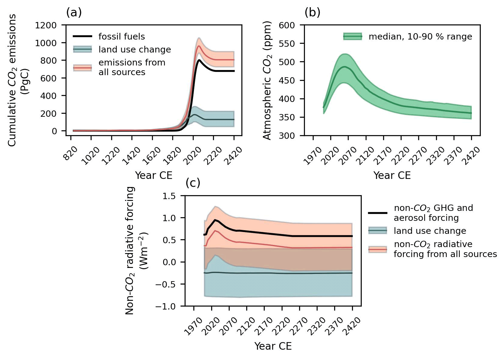
Figure 1 (a) The cumulative CO₂ emissions from 850 CE till the end of the model integration at year 2420; (b) the evolution of the atmospheric CO₂; (c) non-CO₂ radiative forcing from all sources (non-CO₂ greenhouse gas (GHG) and aerosol forcing and land use change) from the year 2000 for the SSP1-2.6 scenario. Solid lines show the median values, and shaded areas indicate the values between the 10th and 90th percentiles.

Simulations start from pre-industrial spin-ups (Holden et al., 2013b) and follow historical transient forcing from 850 to 2005 CE (Eby et al., 2013). In this setting, the land use change emissions start from 850 CE and emissions from other sources including fossil fuels are introduced from 1750 CE. The historical forcing includes CO₂ emissions, non-CO₂ radiative forcings and land use changes, including both anthropogenic and natural sources (volcanic eruptions and solar variability). In order to meld the spin using RCP2.6 at year 2005 with the projected scenario SSP1-2.6, a constant adjustment of 0.446 W m⁻² was added to the non-CO₂ radiative forcing. This adjustment can be viewed as representing contributions from land use change albedo (explicitly modelled in GENIE-1, Fig. 1c) and from non-anthropogenic forcings, which were modelled in the historical spin-up (Eby et al., 2013), comprising volcanic forcing of 0.184 W m⁻² and solar forcing of 0.059 W m⁻² in 2005.

The future forcing scenario (2005 to 2420) follows SSP1-2.6 (Riahi et al., 2017) to the year 2100 and is extended to 2420. Negative emissions are applied as a reduction in anthropogenic CO₂ emissions from the late 2020s, giving net negative emissions from 2077. To extend the SSP1-2.6 from 2100, we follow a similar protocol to Meinshausen et al. (2020). Land use change CO₂ emissions are reduced to zero by 2150 with non-CO₂ land use emissions held fixed from 2100. Fossil fuel emissions, including non-CO₂ greenhouse gases, and negative CO₂ emissions are all brought to zero by 2250 (Fig. 1a and c). This protocol differs slightly from Meinshausen et al. (2020), who reduce negative emissions to zero by 2200; we prefer to avoid a second period of positive emissions from 2200 to 2250. Therefore, we have three CO₂ emission phases: positive emissions from 2020 to 2077, net negative emissions from 2077 to 2250 and zero emissions from 2250 to 2420 (Fig. 1a).

We assume that the carbon removed through negative emissions leaves the system permanently, which is the representation of NETs with long-lived and permanent carbon storage such as carbon capture and storage. This assumption also approximates enhanced rock weathering, although the chemical effects of weathering products are neglected, such as the effect of bicarbonate changes on ocean biogeochemistry which drive co-benefits for the ocean and marine ecosystems (Vakilifard et al., 2021).

To quantify the uncertainty in climate and carbon-cycle responses, we used an 86-member ensemble, a subset of a calibrated 471-member ensemble varying 28 model parameters (Holden et al., 2013a). The selection of 24 of these parameters (Holden et al., 2013b) covers oceanic, atmospheric, sea-ice, ocean biogeochemistry and terrestrial vegetation processes that are thought to contribute to variability in atmospheric CO₂ on glacial–interglacial timescales (Kohfeld and Ridgwell, 2009). The remaining 4 parameters are relevant to the modern state of the climate carbon cycle, describing uncertainties in soil under land management, crop albedo, climate sensitivity and CO₂ fertilisation. The 86 ensemble members are perturbed to cover uncertainty in the 28 parameters and are all constrained to simulate plausible pre-industrial values of global temperature, Atlantic overturning circulation, sea-ice coverage, vegetative and soil carbon, sedimentary calcium carbonate, and dissolved ocean oxygen (Holden et al., 2013b). They additionally simulate reasonable values of atmospheric CO₂ at snapshots (1620, 1770, 1850, 1970 and 2005 CE) through the historical transient period (Foley et al., 2016). The varied parameters are summarised in the Supplement in Table S4 and are fully detailed, along with the ensemble design methodology, in Holden et al. (2013a, b).

4 GENIE-1 model responses

The GENIE-1 model responses are next described in terms of the spread of ensemble responses and the essentials of the carbon and thermal responses.

4.1 Characterising the model ensemble

There are a wide range of responses within the ensemble members making up the model projections following the future forcing scenario SSP1-2.6. At the end of the positive emission phase at the year 2077, the increase in surface air temperature ranges from 1.5 to 4.2 K, the Atlantic meridional overturning circulation change from −12.3 to 0.6 Sv, the land carbon change from a loss of 78 PgC to a gain of 488 PgC and the ocean carbon uptake from a gain of 247 to 586 PgC (Fig. 2).

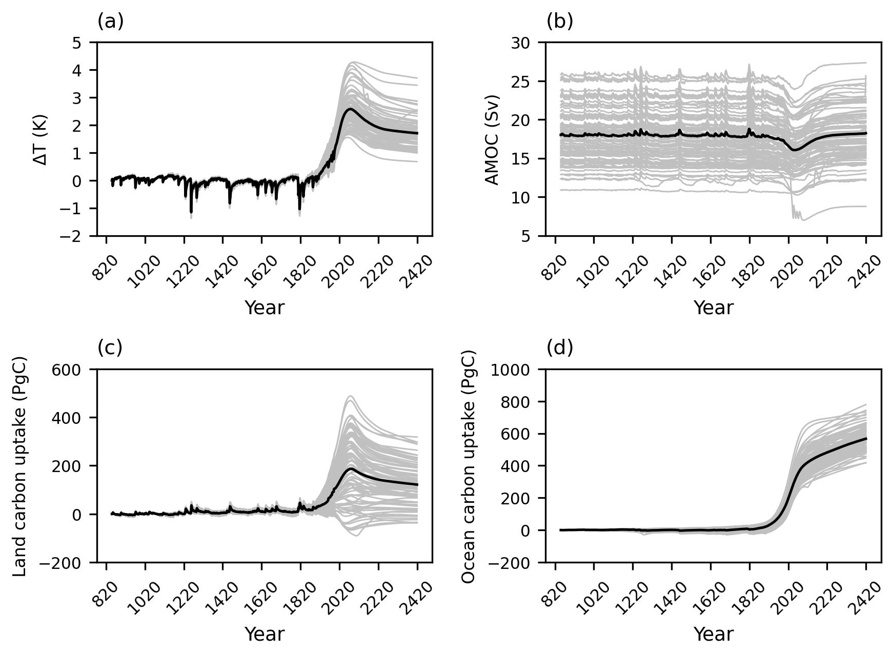
Figure 2 Inter-model spread of 86-member ensemble for change in (a) the surface air temperature, (b) Atlantic meridional overturning circulation (AMOC), (c) the land carbon pool and (d) the ocean carbon pool from the year 850 CE until the year 2420 following the SSP1-2.6 scenario. Black lines show the mean values.

Figure 3 The ensemble average change in the major carbon inventories from 850 CE until the year 2420 for the SSP1-2.6 scenario.

4.2 Carbon response

The distribution of carbon between carbon inventories is diagnosed (Fig. 3), and carbon conservation ensures that at all times the sum of the change in the carbon content of the atmosphere, ΔI_atmos(t); ocean, ΔI_ocean(t); land, ΔI_land(t); and ocean sediment, ΔI_sediment(t), equals the cumulative CO₂ emissions from both land use change and fossil fuels, I_em(t), with all inventories in petagrams of carbon (PgC):

$$\begin{array}{}\text{(10)}& \begin{array}{rl}\mathrm{\Delta }{I}_{\mathrm{atmos}}\left(t\right)& +\mathrm{\Delta }{I}_{\mathrm{ocean}}\left(t\right)+\mathrm{\Delta }{I}_{\mathrm{land}}\left(t\right)\\ & +\mathrm{\Delta }{I}_{\mathrm{sediment}}\left(t\right)=I_{\mathrm{em}}\left(t\right).\end{array}\end{array}$$

Aside from the ocean sediments, which lose carbon, there is an increase in the carbon content of all inventories between the years 2020 and 2077, the positive emission phase (Fig. 3). During this emission phase, the carbon release from the sediment reservoir is ∼ 14 PgC on average, equivalent to a sedimentary CaCO₃ dissolution flux of ∼ 21 TmolC yr⁻¹ and consistent with Archer (1996), Ridgwell and Hargreaves (2007), and Sulpis et al. (2018). The application of carbon capture and storage from the year 2077 decreases the total carbon inventory until the year 2250. During the zero emission phase, the increase in ocean storage is associated with a decrease in carbon content in the atmosphere, land and sediment.

4.3 Thermal response

For the thermal analysis, a global energy balance (Eq. 5) is diagnosed, $\mathrm{\Delta }F\left(t\right)=N\left(t\right)+\mathit{\lambda }\left(t\right)\mathrm{\Delta }T\left(t\right)$, in which the energy balance is expressed as the relationship between radiative forcing, ΔF(t) (W m⁻²); planetary heat uptake, N(t) (W m⁻²); and radiative response, λ(t)ΔT(t) (W m⁻²).

The radiative forcing, ΔF(t), is the sum of non-CO₂ radiative forcing (including land use change albedo) and CO₂ radiative forcing. The non-CO₂ radiative forcing, $\mathrm{\Delta }{F}_{\mathrm{non}-{\mathrm{CO}}_{\mathrm{2}}}\left(t\right)$ (W m⁻²), is a prescribed model forcing input, besides land use change, which is diagnosed as the change in reflected surface insolation under land use change relative to that with natural vegetation, averaged annually across all grid cells. The land use change maps were also fixed from the year 2005, and these were associated with a global forcing of −0.53 to 0.05 W m⁻² (25th- to 75th-percentile range) and mean and median values of −0.23 and −0.26 W m⁻², respectively, across the ensemble. The uncertainty is driven primarily by crop albedo, which varies between 0.12 and 0.18 across the ensemble (Holden et al., 2013a). The CO₂ radiative forcing, $\mathrm{\Delta }{F}_{{\mathrm{CO}}_{\mathrm{2}}}\left(t\right)$ (W m⁻²), was calculated individually for each simulation based on the atmospheric CO₂ concentration (C(t) (ppm)) as outlined in IPCC (2001):

$$\begin{array}{}\text{(11)}& \mathrm{\Delta }{F}_{{\mathrm{CO}}_{\mathrm{2}}}\left(t\right)=\mathit{\alpha }\ln \left({\displaystyle \frac{\mathrm{C}\left(t\right)}{\mathrm{C}\left(t_{\mathrm{0}}\right)}}\right),\end{array}$$

where α is a constant equal to 5.35 W m⁻² and C(t₀) equals 278 ppm.

The ocean heat uptake is used to represent the planetary heat uptake as the model ocean is the principal energy sink and the model does not take into account the energy stored in the lithosphere or consumed in the melting of the ice sheets. In comparison, in the real world, the ocean is responsible for storing over 90 % of the Earth's total energy increase (Church et al., 2011). The climate feedback parameter, λ(t) (W m⁻² K⁻¹), is diagnosed from the ocean heat uptake and the change in global mean surface air temperature (Eq. 5). Most of the radiative forcing drives a radiative response involving a rise in surface air temperature, rather than an increase in ocean heat uptake (Fig. 4).

5 Model responses in terms of climate metrics

The climate response of the GENIE-1 model projections for positive and negative emissions is next assessed in terms of the response of two climate metrics, the effective transient climate response to cumulative CO₂ emissions (eTCRE) and the effective zero emissions commitment (eZEC), as well as in terms of identifying the asymmetrical response to positive and negative emissions.

The results of GENIE-1 simulations show a linear relationship between the change in the surface air temperature and cumulative CO₂ emissions over the positive emission phases (Fig. 5), with the slopes of this relationship varying between ∼ 1.62 and 3.42 K EgC⁻¹ (based on the 10th- and 90th-percentile values). The range of slopes of the ΔT-versus-I_em curve, calculated by linear regression, over the net negative emission phase is larger than in the positive emission phase by a factor of ∼ 2 due to a decrease in non-CO₂ radiative forcing leading to additional cooling during this period. Over this emission phase, the warming relationship is not linear in all ensemble members and exhibits a hysteresis behaviour, as previously identified in Zickfeld et al. (2016), Jeltsch-Thömmes et al. (2020) and Koven et al. (2022). Differences in the rates of surface air temperature change over the net negative emission phase are mainly due to the terrestrial carbon uncertainty (discussed in Sect. 4.2.2).

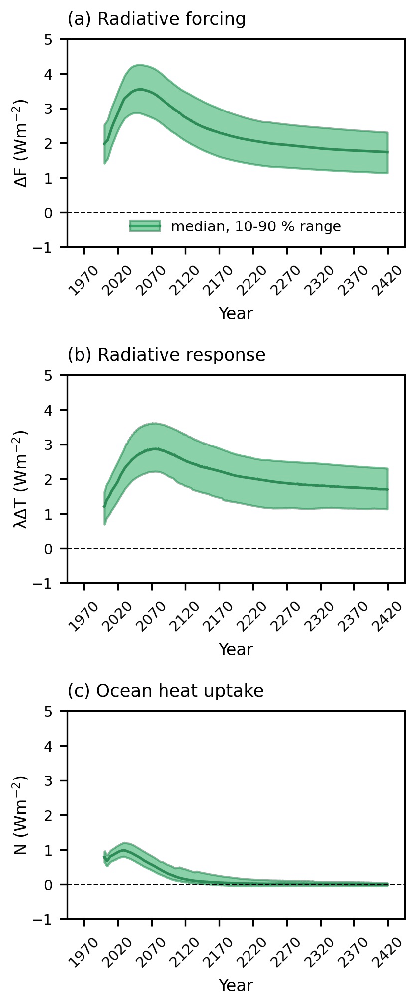
Figure 4 The evolution of (a) radiative forcing, (b) radiative response and (c) ocean heat uptake in the SSP1-2.6 scenario from the year 2000. Solid lines show the median values, and shaded areas indicate the values between the 10th and 90th percentiles.

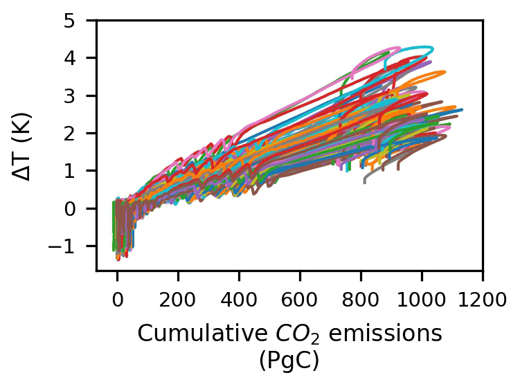
Figure 5 Change in the surface air temperature versus cumulative CO₂ emissions from 850 CE until the year 2420 in the SSP1-2.6 scenario.

5.1 Drivers of the effective transient climate response to cumulative CO₂ emissions

Following Sect. 2, the effective transient climate response to cumulative CO₂ emissions (eTCRE) is evaluated in terms of the product of (i) the dependence of surface warming on the radiative forcing, referred to as the thermal dependence, $\mathrm{\Delta }T\left(t\right)/\mathrm{\Delta }F\left(t\right)$; (ii) the dependence of the radiative forcing on the cumulative CO₂ emissions, referred to as a radiative dependence, $\mathrm{\Delta }F\left(t\right)/\mathrm{\Delta }{I}_{\mathrm{atmos}}\left(t\right)$; and (iii) the airborne fraction, $\mathrm{\Delta }{I}_{\mathrm{atmos}}\left(t\right)/I_{\mathrm{em}}\left(t\right)$, referred to as a carbon dependence (Eq. 9):

$$\begin{array}{rl}& \mathrm{eTCRE}\equiv {\displaystyle \frac{\mathrm{\Delta }T\left(t\right)}{I_{\mathrm{em}}\left(t\right)}}=\\ & \underset{\mathrm{thermal}}{\underbrace{\left({\displaystyle \frac{\mathrm{\Delta }T\left(t\right)}{\mathrm{\Delta }F\left(t\right)}}\right)}}\underset{\mathrm{radiative}\mathrm{from}{\mathrm{CO}}_{\mathrm{2}}\mathrm{and}\text{non-}{\mathrm{CO}}_{\mathrm{2}}}{\underbrace{\left({\displaystyle \frac{\mathrm{\Delta }F\left(t\right)}{\mathrm{\Delta }{F}_{{\mathrm{CO}}_{\mathrm{2}}}\left(t\right)}}\right)\left({\displaystyle \frac{\mathrm{\Delta }{F}_{{\mathrm{CO}}_{\mathrm{2}}}\left(t\right)}{\mathrm{\Delta }{I}_{\mathrm{atmos}}\left(t\right)}}\right)}}\underset{\mathrm{carbon}}{\underbrace{\left({\displaystyle \frac{\mathrm{\Delta }{I}_{\mathrm{atmos}}\left(t\right)}{\mathrm{\Delta }{I}_{\mathrm{em}}\left(t\right)}}\right)}}.\end{array}$$

The model ensemble reveals a decrease in the eTCRE from the median value of 2.71 K EgC⁻¹ in the year 2020 to 2.0 K EgC⁻¹ in the year 2420 (with 10 %–90 % ranges of 2.0 to 3.65 and 1.39 to 2.96 K EgC⁻¹, respectively) (Fig. 6a). During the positive emission phase (to the year 2077) this reduction is driven by a weakening in the radiative forcing with an increase in atmospheric carbon (Fig. 6b), which dominates over the increase in the thermal dependence (Fig. 6d). During the net negative and zero emission phases (from the year 2077), the eTCRE reduction is driven by the reducing airborne fraction as CO₂ is drawn down by the ocean (Fig. 6e).

The eTCRE is scenario dependent and varies with both CO₂ and non-CO₂ portions of the radiative forcing. Following the analysis of Matthews et al. (2021), we quantify the spread of the non-CO₂ fraction of total anthropogenic forcing, f_nc (from Eq. 8), between 2020 and 2100 (Table S1) to investigate the extent of scenario dependency of the eTCRE. The results show that the f_nc range varies from ∼ 10 % to ∼ 26 % (25th- to 75th-percentile values) in 2020 to ∼ 5 % to ∼ 21 % in 2100, corresponding to a ∼ 6 % decrease (mean value) over the course of 80 years. The TCRE diagnosed by removing the non-CO₂ warming factor (from Eq. 8) remains constant at ∼ 2.2 K EgC⁻¹ (median values) over the entire period. However, the uncertainty increases towards the end of the century, varying from 1.75 to 2.82 K EgC⁻¹ (10th- to 90th-percentile values) in 2020 to up to ∼ 3.13 K EgC⁻¹ in 2100 (Fig. S1).

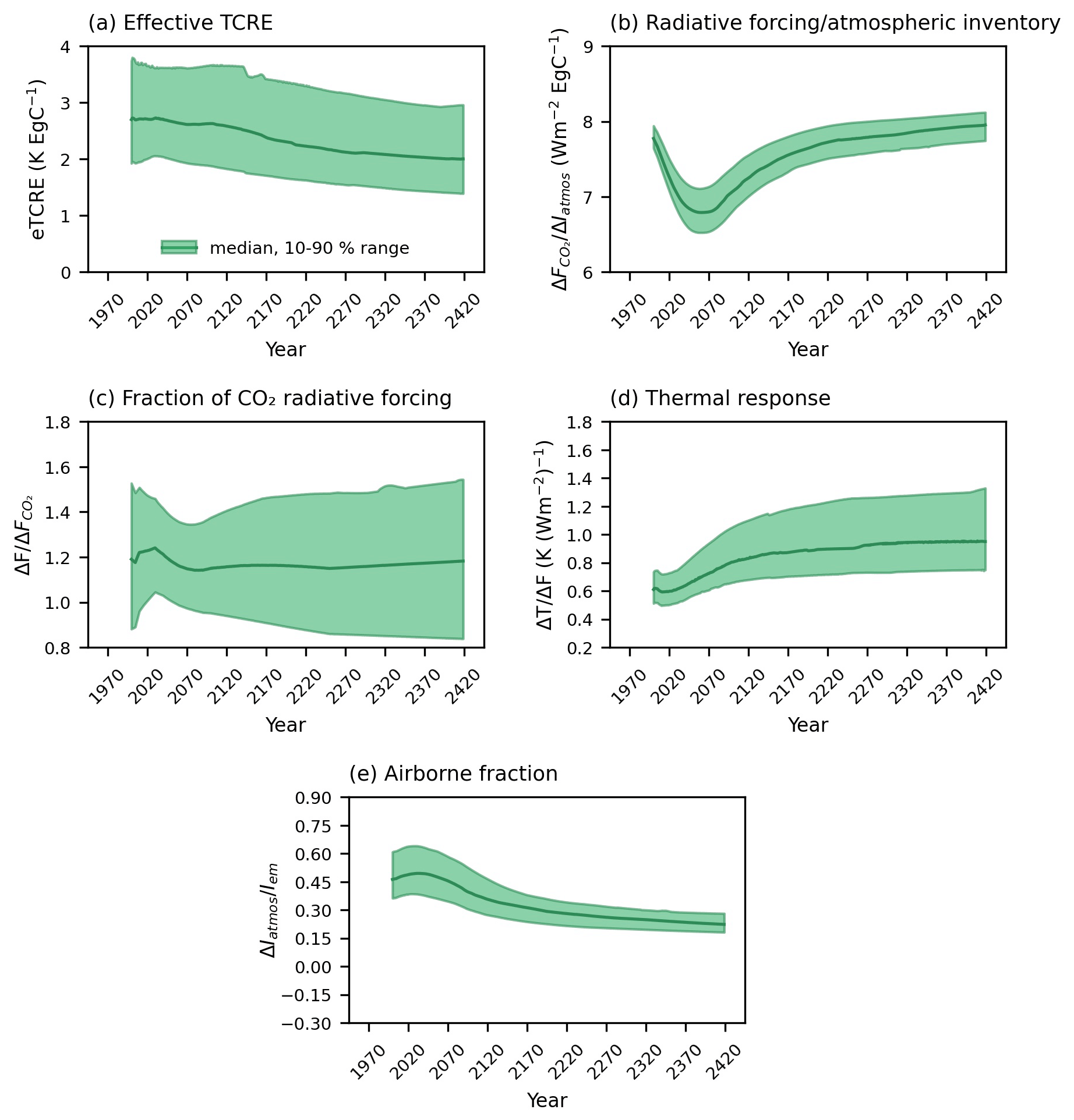
Figure 6 Effective transient climate response to cumulative CO₂ emissions (eTCRE) and its components for the SSP1-2.6 scenario from the year 2000: (a) eTCRE, (b) dependence of the radiative forcing on atmospheric CO₂, (c) fractional radiative-forcing contribution from atmospheric CO₂, (d) thermal dependence and (e) airborne fraction. Solid lines show the median values, and shaded areas indicate the values between the 10th and 90th percentiles.

The uncertainty in the eTCRE, as well as its dependencies for the model ensemble, is assessed based on the non-dimensional coefficient of variation, given by the inter-model standard deviation divided by the ensemble mean (Williams et al., 2020). The uncertainty in the eTCRE varies from 0.23 to 0.3 over the course of the model integrations and is larger by 0.05 for the net negative emission phase compared to the positive emission phase (Table 1).

During the positive and net negative emissions, the coefficients of variation for the thermal dependence (∼ 0.18 to ∼ 0.2) and airborne fraction (∼ 0.2) provide the dominant contributions to the eTCRE uncertainty (Table 1). During the zero emission phase, however, the coefficient of variation for the fractional radiative-forcing contribution from atmospheric CO₂, $\mathrm{\Delta }F\left(t\right)/\mathrm{\Delta }{F}_{{\mathrm{CO}}_{\mathrm{2}}}\left(t\right)$(∼ 0.22), is larger than the contribution from the airborne fraction (∼ 0.16). In all emission phases, the dependence of the radiative forcing on atmospheric CO₂, $\mathrm{\Delta }{F}_{{\mathrm{CO}}_{\mathrm{2}}}\left(t\right)/\mathrm{\Delta }{I}_{\mathrm{atmos}}\left(t\right)$, has the least contribution to the eTCRE uncertainty (∼ 0.02).

Table 1 Effective transient climate response to cumulative CO₂ emissions (eTCRE) and its components for the different emission phases in the SSP1-2.6 scenario. The coefficient of variation (${\mathit{\sigma }}_x/\stackrel{\mathrm{‾}}{x})$ is defined by the inter-model standard deviation (σ_x) divided by the inter-model mean ($\stackrel{\mathrm{‾}}{x})$.

5.1.1 Carbon dependence for the effective transient climate response to cumulative CO₂ emissions

The fraction of emitted CO₂ that remains in each carbon inventory (based on Eq. 7) varies over the course of the integrations. The carbon dependence for the eTCRE is given by the airborne fraction of carbon emissions, $\mathrm{\Delta }{I}_{\mathrm{atmos}}\left(t\right)/I_{\mathrm{em}}\left(t\right)$. By the year 2077, the end of the positive emission phase, the atmosphere is the largest carbon sink with an airborne fraction of ∼ 49 % (mean value) (Fig. 7a and Table S2). After the year 2077, during the net negative and zero emission phases, the ocean becomes the dominant carbon sink with an increase in the ocean-borne fraction, $\mathrm{\Delta }{I}_{\mathrm{ocean}}\left(t\right)/I_{\mathrm{em}}\left(t\right)$, up to ∼ 67 % (mean value) by 2420 (Fig. 7b and Table S2). The land-borne fraction, $\mathrm{\Delta }{I}_{\mathrm{land}}\left(t\right)/I_{\mathrm{em}}\left(t\right)$, decreases from ∼ 19 % (mean value) in 2020 to the minimum value of ∼ 15 % in 2420 (Fig. 7c and Table S2). The sediment-borne fraction, $\mathrm{\Delta }{I}_{\mathrm{sediment}}\left(t\right)/I_{\mathrm{em}}\left(t\right)$, remains negative at ∼ −0.04 (mean value) over the entire period (Fig. 7d and Table S2) and therefore acts as a weak carbon source.

The coefficient of variation is the largest for the land-borne fraction (∼ 0.7), followed by the sediment-borne fraction (∼ −0.5) and then the airborne and ocean-borne fractions, decreasing from ∼ 0.2 over the positive emission phase to ∼ 0.15 during the zero emission phase (Table S2). The main contribution to the model ensemble spread is, therefore, the land carbon system.

Figure 7 The evolution of the (a) airborne fraction, (b) ocean-borne fraction, (c) land-borne fraction and (d) sediment-borne fraction in the SSP1-2.6 scenario. Note that the y axis shows the cumulative fraction of CO₂ which remains in each carbon inventory. Solid lines show the median values, and shaded areas indicate the values between the 10th and 90th percentiles from the year 2000.

5.1.2 Radiative-forcing dependence for the effective transient climate response to cumulative CO₂ emissions

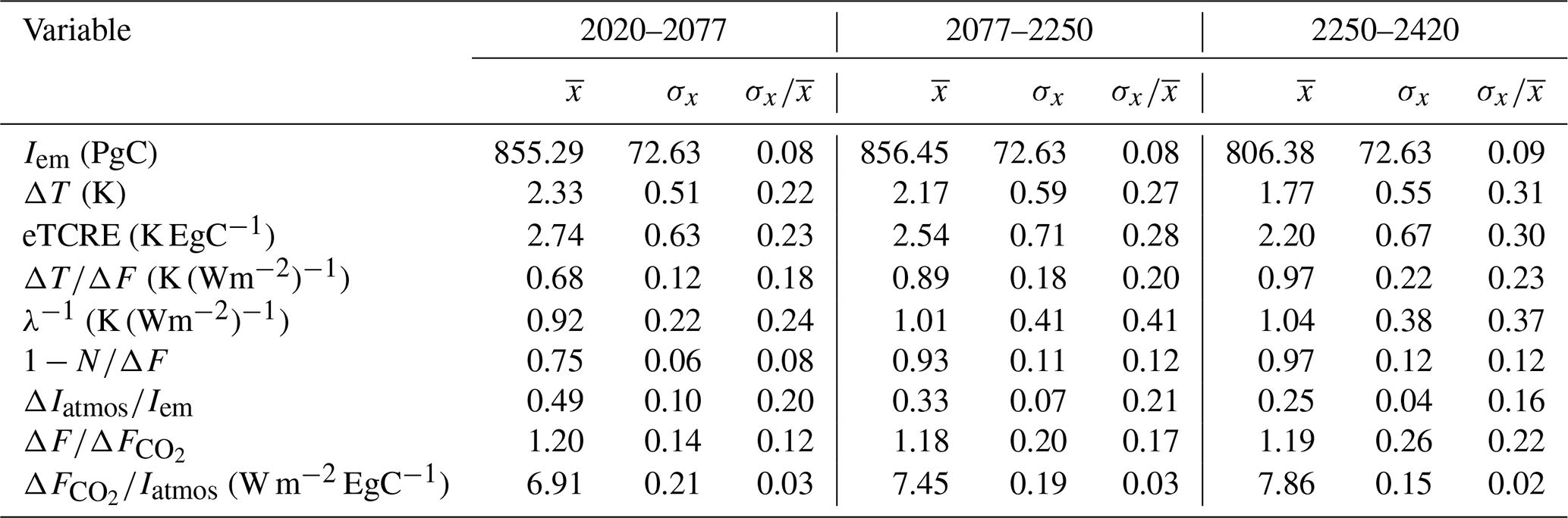
By the end of the positive emissions at year 2077, the radiative-forcing dependence on atmospheric CO₂ emissions, $\mathrm{\Delta }F\left(t\right)/\mathrm{\Delta }{I}_{\mathrm{atmos}}\left(t\right)$, weakens due to a saturation in the radiative forcing with an increase in atmospheric CO₂ (Gillett et al., 2013; William et al., 2020) (Figs. 1b and 8b). During the net negative emissions and zero emission phases over the next few centuries from the year 2077 onwards, $\mathrm{\Delta }F\left(t\right)/\mathrm{\Delta }{I}_{\mathrm{atmos}}\left(t\right)$ rises again due to a decrease in atmospheric CO₂ associated with the decrease in the airborne fraction (Fig. 8c).

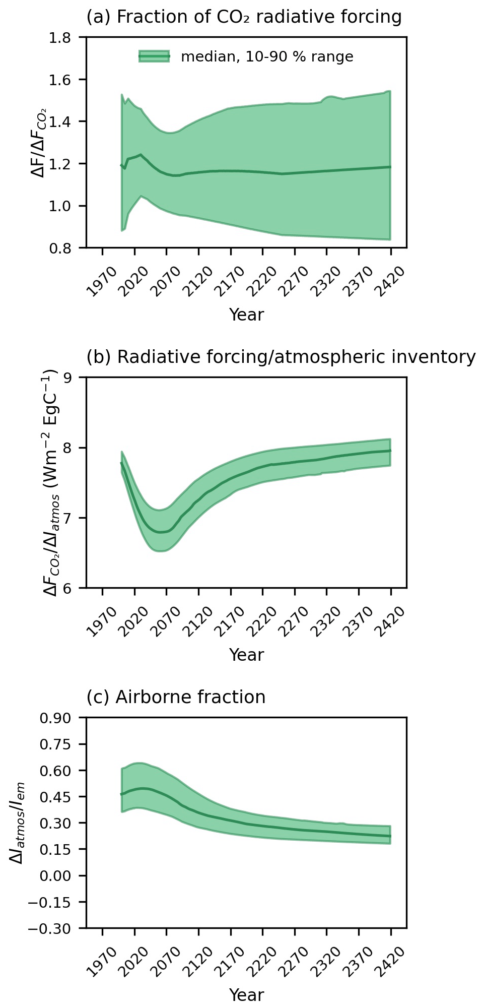
Figure 8 Radiative-forcing dependence for the effective TCRE and its components in the SSP1-2.6 scenario from the year 2000. (a) Fractional radiative-forcing contribution from atmospheric CO₂; (b) dependence of the radiative forcing on atmospheric CO₂; (c) airborne fraction. Solid lines show the median values, and shaded areas indicate the values between the 10th and 90th percentiles.

5.1.3 Thermal dependence for the effective transient climate response to CO₂ emissions

The thermal dependence of the eTCRE, involving the dependence of the surface warming on the radiative forcing, $\mathrm{\Delta }T\left(t\right)/\mathrm{\Delta }F\left(t\right)$, increases in all emission phases (Fig. 9a) due to the reinforcing contributions of the inverse of the climate feedback parameter, λ(t)⁻¹ (Fig. 9b), and the fraction of the radiative forcing warming the surface, $\mathrm{1}-N\left(t\right)/\mathrm{\Delta }F\left(t\right)$ (Fig. 9c). The increase in λ(t)⁻¹ is equivalent to a slight decrease in the climate feedback λ(t). The temporal evolution of the climate feedback parameter is mirrored in other climate model studies as climate feedbacks evolve on different timescales according to the nature of the controlling processes (Gregory et al., 2004; Armour et al., 2013; Knutti and Rugenstein, 2015; Goodwin, 2018). The fraction of the radiative forcing warming the surface increases by ∼ 22 % (based on the mean values, Table 1) from the year 2020 to the year 2420 with a corresponding reduction in the heat transfer into the deep ocean; by the year 2420, nearly all the radiative forcing is warming the surface with the ratio $\mathrm{1}-N\left(t\right)/\mathrm{\Delta }F\left(t\right)$ reaching 0.97 (mean values, Table 1) (Fig. 9c–d). This response is probably due to an increase in ocean stratification from the rise in surface ocean temperature (Figs. S2–S4) from the increased radiative forcing.

The coefficient of variation for the thermal dependence remains ∼ 0.2 over the entire period (Table 1). Within the thermal dependence, the term relating to the climate feedback parameter λ(t)⁻¹ has a coefficient of variation more than ∼ 3 times that of the fraction of the radiative forcing warming the surface $\mathrm{1}-N\left(t\right)/\mathrm{\Delta }F\left(t\right)$ (Table 1). As the thermal-dependence terms, λ(t)⁻¹ and $\mathrm{1}-N\left(t\right)/\mathrm{\Delta }F\left(t\right)$, are strongly anti-correlated (Fig. S5), the relative spread in the thermal response is thus mitigated by the feedback between the climate feedback parameter and the fraction of the radiative forcing warming the surface.

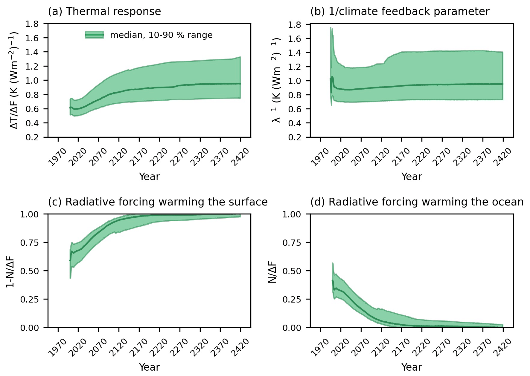
Figure 9 The evolution of (a) thermal dependence for the effective TCRE given by the dependence of the surface warming on the radiative forcing, $\mathrm{\Delta }T\left(t\right)/\mathrm{\Delta }F\left(t\right)$, and the contributions from (b) the inverse of the climate feedback, (c) the fraction of the radiative forcing warming the surface and (d) the fraction of the radiative forcing warming the ocean interior in the SSP1-2.6 scenario from the year 2000. Solid lines show the median values, and shaded areas indicate the values between the 10th and 90th percentiles.

5.2 The asymmetry of the Earth system response to positive and negative emissions

5.2.1 Hysteresis

The relationship between the surface air temperature and atmospheric CO₂ exhibits hysteresis behaviour in most ensemble members, consistent with climate change reversibility studies (Fig. 10a) (Tokarska and Zickfeld, 2015; Jeltsch-Thömmes et al., 2020). The temperature remains at high levels after high atmospheric CO₂, concurrently with a decrease in the ocean heat uptake, N(t) (Fig. 10b). The ability of the ocean interior to take up heat diminishes in time, probably due to increasing stratification and weakening ventilation. The fraction of the radiative forcing warming the ocean interior, $N\left(t\right)/\mathrm{\Delta }F\left(t\right)$ (Fig. 10c), then continues to decrease after the peak in atmospheric CO₂, leading to higher surface air temperatures even after the lower CO₂ concentrations are restored.

The atmospheric CO₂ declines during the net negative emission phase from the year 2077 (Fig. 1b) associated with the cumulative CO₂ emissions of ∼ 960.4 PgC (median value) (Figs. 1a and 10d). After the cessation of the emissions, the atmospheric CO₂ continues to decrease (Fig. 10d) mainly due to uptake by the ocean and to a lesser extent the land (Fig. 10e–f). The ocean carbon uptake is governed by the air–sea flux of CO₂ and thermocline ventilation, with uncertainties dominated by ventilation processes transferring carbon from the surface ocean to the main thermocline and deep ocean (Holden et al., 2013b; Goodwin et al., 2015; Zickfeld et al., 2016; Jeltsch-Thömmes et al., 2020). The ocean continues to take up carbon after the peak in atmospheric CO₂ as there is continuing long-term adjustment and ventilation of the deep ocean (Fig. 10e). The complex responses of land carbon (Fig. 10f) are driven by a range of competing processes, most notably carbon uptake through CO₂ fertilisation and the carbon release through historical land use changes and accelerated respiration under warming.

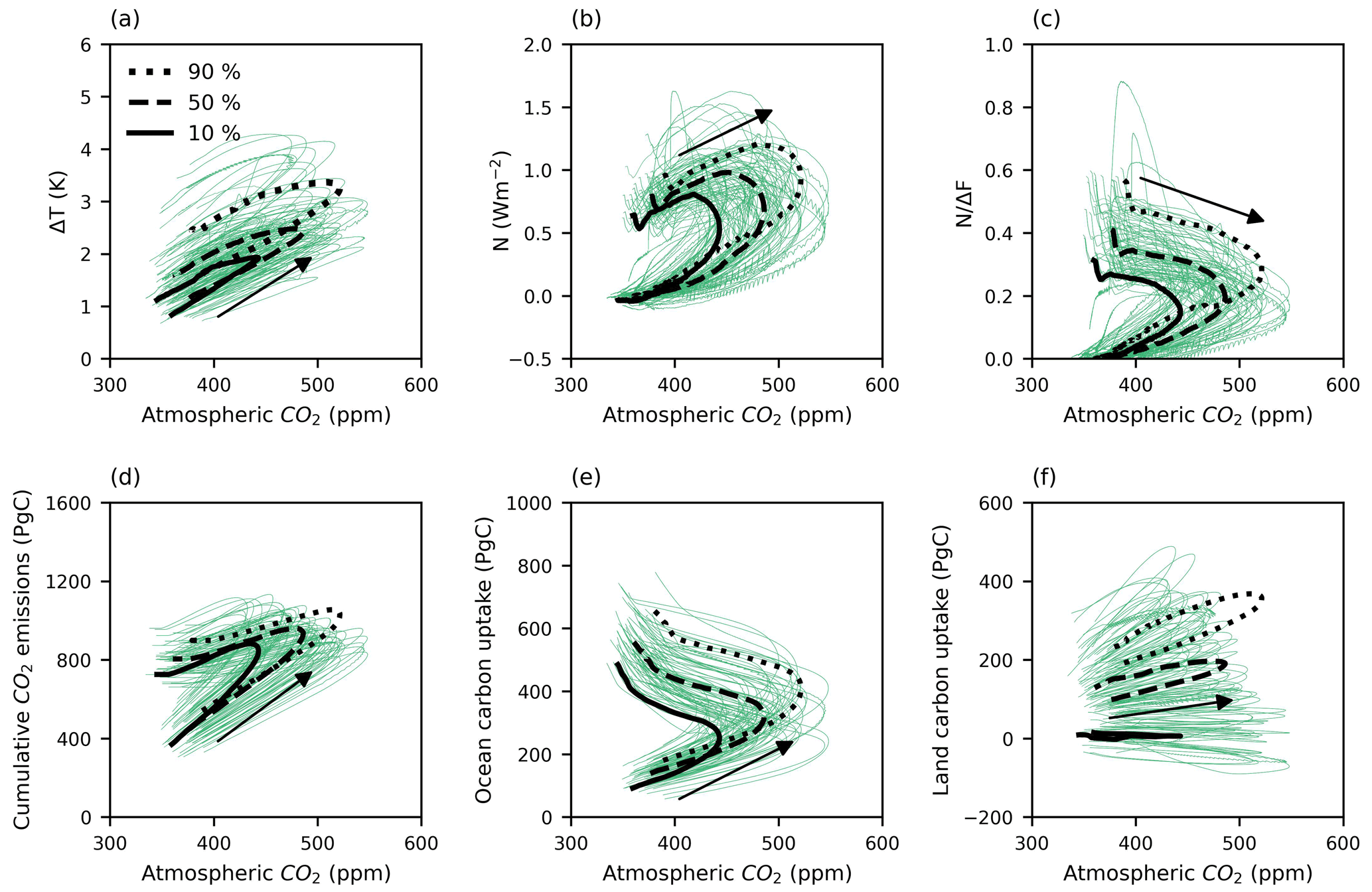
Figure 10 The thermal (upper row) and carbon (lower row) variables versus atmospheric CO₂ in the SSP1-2.6 scenario from the year 2000. (a) Change in surface air temperature; (b) ocean heat uptake; (c) fraction of the radiative forcing warming the ocean interior; (d) cumulative CO₂ emissions; (e) change in the ocean carbon pool; (f) change in the land carbon pool. In each panel the black lines show the median and 10th- and 90th-percentile values of the atmospheric CO₂ versus the median and 10th- and 90th-percentile values of the thermal and carbon variables.

5.2.2 Correlation between the model parameters and the slope of the change in surface air temperature versus cumulative CO₂ emissions ($\mathrm{\Delta }T/\mathrm{\Delta }{I}_{\mathrm{em}})$

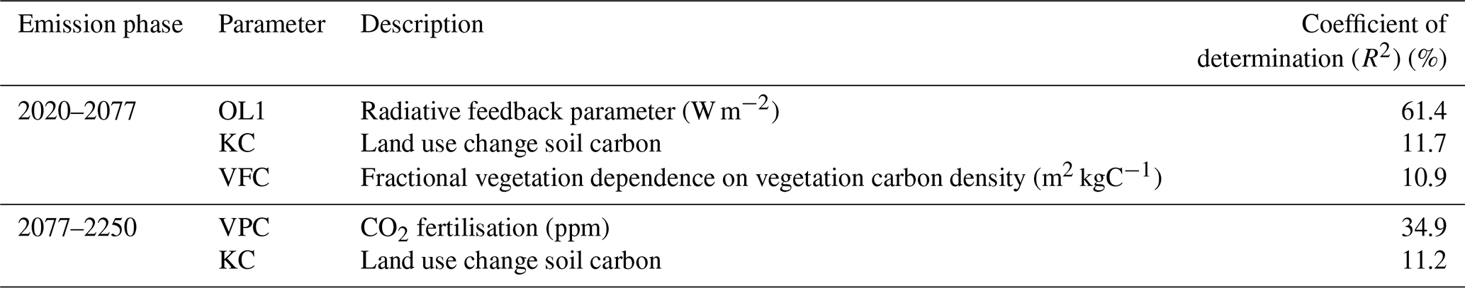
We calculated the coefficients of determination (R²) between $\mathrm{\Delta }T/\mathrm{\Delta }{I}_{\mathrm{em}}$ and the 28 model parameters across the ensemble during both positive and net negative emission phases. For this purpose, 4 of the 86 simulations were omitted as outliers because they were undergoing substantial re-organisation of ocean circulation during the period of net negative emissions (Fig. S6), significantly perturbing ocean heat uptake.

During the positive emission phase, uncertainty in $\mathrm{\Delta }T/\mathrm{\Delta }{I}_{\mathrm{em}}$ is dominated by the radiative feedback parameter (OL1) (R² ∼ 61 %) (Table 2), which perturbs outgoing longwave radiation proportionally to ΔT (Matthews and Caldeira, 2007). This parameter is primarily designed to capture unmodelled cloud responses to global average temperature change, and it has previously been shown to drive 81 % of the variance in GENIE-1 climate sensitivity (Holden et al., 2010). The parameter links to the climate feedback parameter in the eTCRE framework (Sect. 4.1), which was shown to be the dominant driver of uncertainty in the thermal response and therefore eTCRE values.

Although radiative-forcing uncertainty dominates, carbon-cycle parameters also drive $\mathrm{\Delta }T/\mathrm{\Delta }{I}_{\mathrm{em}}$ variance via the land use change soil carbon parameter (KC) (R² ∼ 12 %) through its control on soil carbon losses under land use change. The fractional vegetation parameter (VFC) (R² ∼ 11 %) drives additional carbon-cycle uncertainty through its control on terrestrial carbon surface density. The results are associated with the airborne fraction in the eTCRE framework, diagnosed as another factor controlling the uncertainty in the eTCRE during this emission phase (Sect. 4.1).

During net negative emissions (2077–2250), uncertainty in $\mathrm{\Delta }T/\mathrm{\Delta }{I}_{\mathrm{em}}$ is affected mainly by the CO₂ fertilisation (VPC) (R² ∼ 35 %), which is a major source of terrestrial carbon uncertainty, and to a lesser extent the parameter that controls the rate of carbon loss from soils under land use change (KC, ∼ 11 %). The effect of the carbon contribution in the uncertainty is expressed through the airborne fraction in the eTCRE framework, which was revealed to be the main reason behind the large spread of the eTCRE over the net negative emission phase (Sect. 4.1), consistent with MacDougall et al. (2017).

Table 2 Correlation between model parameters and $\mathrm{\Delta }T/\mathrm{\Delta }{I}_{\mathrm{em}}$ in the SSP1-2.6 scenario over different emission phases based on the coefficients of determination (R²) (%). R²>50 % denotes strong correlation and R²>10 % moderate correlation. The values less than 10 % are shown in Table S3.

5.3 The effective zero emissions commitment

The zero emissions commitment (ZEC) is now assessed, given by the mean surface air temperature change after CO₂ emissions cease (Hare and Meinshausen, 2006; Matthews and Caldeira, 2008; Froelicher and Paynter, 2015; MacDougall et al., 2020). Whether there is continued surface warming depends on competition between a cooling effect from reduction in atmospheric CO₂ due to the ocean and land sequestration of carbon and a surface warming effect from a decline in the heat uptake by the ocean interior (Williams et al., 2017b).

In our analysis, we define the effective ZEC (eZEC), which assesses the continued surface warming after the cessation of CO₂ emissions while the non-CO₂ greenhouse gas and aerosol forcings evolve. Our reference scenario applies SSP1-2.6 CO₂ emissions until the year 2077 and zero emissions thereafter, with cumulative emissions of ∼ 961 PgC (median value) (Fig. S7). Following the analysis of MacDougall et al. (2020), we define eZEC₂₅, eZEC₅₀ and eZEC₉₀ as the mean surface air temperature anomalies at the 25th, 50th and 90th years after the cessation of emissions to account for the implications of the eZEC over a range of multi-decadal timescales relevant to climate policy.

Diagnosed eZEC values are illustrated in Fig. 11 (the reference plotted as orange bars). In the reference scenario, the distribution of the eZEC displays an uncertain sign. There is a temperature overshoot in 20 % of eZEC₂₅ values (10 %–90 % range from −0.08 to 0.02 K) and in 11 % of eZEC₅₀ values (range from −0.17 to 0.01 K) and 5 % of eZEC₉₀ values (range from −0.31 to −0.05 K). The ensemble means of eZEC₂₅, eZEC₅₀ and eZEC₉₀ are −0.03, −0.10 and −0.21 K, respectively, and compare to values of −0.01, −0.07 and −0.12 K in the 1000 PgC experiment of MacDougall et al. (2020) (grey bars). The additional cooling is in part due to ongoing reductions in non-CO₂ forcing from 0.728 W m⁻² in 2077 to 0.648 W m⁻² in 2167 (Fig. 1c), noting that MacDougall et al. (2020) performed an idealised experiment that only considered CO₂ emissions forcing. We realise that our uncertainties are lower than those of MacDougall et al. (2020), which at least in part reflects the absence of internal (decadal) variability in the EMBM of GENIE-1, noting that inter-annual, although not decadal, variability was removed from MacDougall et al. (2020) through 20-year averaging.

In contrast to the reference scenario, surface temperatures decrease in all the ensemble members after cessation of positive emissions in the SSP1-2.6 scenario. We consider two alternative interpretations of the eZEC, the warming after the cessation of positive emissions (in 2077) and the warming after the cessation of net negative emissions (in 2250). The former may be more relevant from a policy perspective (as the time of likely peak warming), while the latter is theoretically useful to quantify committed warming when emissions are precisely zero.

The blue bars in Fig. 11 illustrate the eZEC results for the SSP1-2.6 scenario calculated relative to 2250. There is a temperature overshoot in 5 % of the eZEC₂₅ values; however, the values remain at or below zero within the 10 %–90 % range (−0.06 to 0 K). The values of eZEC₂₅ and eZEC₉₀ are robustly negative, ranging from −0.1 to −0.01 K and −0.16 to −0.03 K (10th- to 90th-percentile range), respectively. Ensemble means are −0.03 K for eZEC₂₅, −0.06 K for eZEC₅₀ and −0.09 K for eZEC₉₀.

The green bars in Fig. 11 illustrate the eZEC values from 2077 (which includes the period of ongoing net negative emissions). The average values of the eZEC are significantly lower than from 2250, being −0.1, −0.26 and −0.47 K, due to the additional cooling driven by net negative emissions. All eZEC values are again robustly negative, varying between −0.14 and −0.05 for eZEC₂₅, −0.34 and −0.16 for eZEC₅₀, and −0.61 and −0.31 for eZEC₉₀ (10th- to 90th-percentile values), confirming that no ensemble member exhibits a temperature overshoot after the cessation of positive emissions.

Figure 11 The distribution of the effective zero emissions commitment (eZEC) in the reference scenario at the 25th, 50th and 90th years relative to the year 2077 (orange bars) and in SSP1-2.6 relative to the year 2250 (blue bars) and relative to the year 2077 (green bars) versus the zero emissions commitment results of MacDougall et al. (2020) (grey bars). The mean values are shown with cross marks. Note that the year 2077 is the end of the positive emission phase and the year 2250 is the end of the net negative emission phase.

6 Conclusions

There is an increasing need to develop and implement carbon capture and sequestration techniques to meet the Paris Agreement 1.5 and 2 ^∘C temperature targets (UNFCCC, 2015). However, it is unclear how these negative emissions affect the climate response, as represented by two key climate metrics: the effective transient climate response to cumulative CO₂ emissions (eTCRE), defining the relationship between surface warming and cumulative CO₂ emissions, and the effective zero emissions commitment (eZEC), defining the anticipated warming after the cessation of CO₂ emissions and continued non-CO₂ greenhouse gas and aerosol forcings. The effect of negative emissions is assessed here using a GENIE-1 ensemble, following SSP1-2.6 with the net negative CO₂ emissions of ∼ 156 PgC over 173 years. The model responses include 86 members that span a wide range of climate and carbon-cycle feedback strengths. The ensemble analysis is enabled by employing low resolution and intermediate complexity, with the most notable simplifications being of the fixed wind-field energy–moisture balance atmosphere, neglecting dynamic atmosphere–ocean feedbacks, and the simple model of terrestrial carbon, which neglects nutrient limitation, does not represent permafrost (or methane) and has a one-level description of soil carbon.

The eTCRE decreases in time due to a combination of the weakening in the radiative forcing with an increase in atmospheric carbon during positive emissions and a reduction in the airborne fraction after emissions cease, which together outweigh the strengthening thermal dependence.

The comparison of the coefficient of variation for the eTCRE and its dependencies shows that the thermal dependence and airborne fraction almost equally contribute to the uncertainty in the eTCRE during the positive emission phase. The results are consistent with those from the model parameter correlation analysis in which different slopes of the change in surface air temperature versus emissions are due to primarily the uncertainty in radiative feedbacks and to a lesser extent carbon-cycle feedbacks. Our results differ from the analyses of CIMIP5 and CMIP6 ensembles in which the radiative-forcing response and thermal response were the main contributors to the uncertainty in the TCRE, respectively (Williams et al., 2020). During the net negative emission phase, both analyses show that the carbon dependence causes the main uncertainty in the values of the eTCRE.

The relationship between thermal and carbon feedbacks with an increase in atmospheric CO₂ exhibits hysteresis behaviour. The fraction of the radiative forcing warming the surface continues to increase after peak atmospheric CO₂ as the ocean is stratified, leading to higher surface air temperatures after lower atmospheric CO₂ values are restored. The increase in the ocean storage after the peak in atmospheric CO₂ is associated with the long-term adjustment and ventilation of the deep ocean, while the reason for the continued terrestrial carbon storage relates to competing processes such as carbon uptake through CO₂ fertilisation and carbon release through historical land use changes and accelerated respiration under warming.

The eZEC is close to zero. In the model mean of the integrations that exclude carbon capture and storage, the eZEC is −0.03 K at 25 years and decreases to −0.21 K at 90 years after emissions cease. However, even assisted by gradual reductions in non-CO₂ forcing as in this scenario, the distribution of the eZEC after 25 years from the cessation of emissions shows continued warming in ∼ 20 % of ensemble members. Including carbon capture and storage reduces the probability of continued warming after net zero, with 95 % ensemble members exhibiting an eZEC close to or below zero. Hence, implementing negative emissions is required to reduce the risk of overshoot and continued warming after net zero is reached and increase the probability of meeting the Paris targets. Negative emissions technologies with naturally long CO₂ removal lifetimes, such as enhanced rock weathering (Beerling et al., 2020), may be especially well suited for this purpose as the legacy effects of the repeated application of this technology increase the rate of carbon drawdown per unit area for years after implementation at no incremental cost (Beerling et al., 2020; Vakilifard et al., 2021).