the Creative Commons Attribution 4.0 License.
the Creative Commons Attribution 4.0 License.
 | 12 Oct 2022
Multi-year observations reveal a larger than expected autumn respiration signal across northeast Eurasia
Brendan Byrne
Junjie Liu
Yonghong Yi
Abhishek Chatterjee
Sourish Basu
Rui Cheng
Russell Doughty
Frédéric Chevallier
Kevin W. Bowman
Nicholas C. Parazoo
David Crisp
Jingfeng Xiao
Stephen Sitch
Bertrand Guenet
Feng Deng
Matthew S. Johnson
Sajeev Philip
Patrick C. McGuire
Charles E. Miller
Site-level observations have shown pervasive cold season CO2 release across Arctic and boreal ecosystems, impacting annual carbon budgets. Still, the seasonality of CO2 emissions are poorly quantified across much of the high latitudes due to the sparse coverage of site-level observations. Space-based observations provide the opportunity to fill some observational gaps for studying these high-latitude ecosystems, particularly across poorly sampled regions of Eurasia. Here, we show that data-driven net ecosystem exchange (NEE) from atmospheric CO2 observations implies strong summer uptake followed by strong autumn release of CO2 over the entire cold northeastern region of Eurasia during the 2015–2019 study period. Combining data-driven NEE with satellite-based estimates of gross primary production (GPP), we show that this seasonality implies less summer heterotrophic respiration (Rh) and greater autumn Rh than would be expected given an exponential relationship between respiration and surface temperature. Furthermore, we show that this seasonality of NEE and Rh over northeastern Eurasia is not captured by the TRENDY v8 ensemble of dynamic global vegetation models (DGVMs), which estimate that 47 %–57 % (interquartile range) of annual Rh occurs during August–April, while the data-driven estimates suggest 59 %–76 % of annual Rh occurs over this period. We explain this seasonal shift in Rh by respiration from soils at depth during the zero-curtain period, when sub-surface soils remain unfrozen up to several months after the surface has frozen. Additional impacts of physical processes related to freeze–thaw dynamics may contribute to the seasonality of Rh. This study confirms a significant and spatially extensive early cold season CO2 efflux in the permafrost-rich region of northeast Eurasia and suggests that autumn Rh from subsurface soils in the northern high latitudes is not well captured by current DGVMs.
- Article
(4871 KB) - Full-text XML
-
Supplement
(13701 KB) - BibTeX
- EndNote


Boreal and Arctic ecosystems hold vast quantities of soil carbon and play an important role in the global carbon cycle (Schuur et al., 2015). These ecosystems are also experiencing the most rapid climate change (Overland et al., 2018), driving major changes in the carbon cycle, including greening trends (Park et al., 2016), permafrost thaw (Schuur et al., 2015; Turetsky et al., 2019, 2020), and increased fire frequency and intensity (Veraverbeke et al., 2017, 2021). Yet, the impact of these changes on the carbon budget of the region remains uncertain (Schuur et al., 2015; McGuire et al., 2018; Miner et al., 2022). In part, this is due to sparse site-level observations in boreal and Arctic ecosystems, while the limited available observations of high-latitude ecosystems are providing surprises.
A synthesis of Arctic and boreal site-level flux measurements from the literature found pervasive CO2 release during the cold season (Natali et al., 2019) such that the cold season is not a dormant period but strongly impacts annual carbon budgets (Zimov et al., 1993; Björkman et al., 2010; Natali et al., 2019). Particularly strong releases of CO2 have been observed during the early cold season (Commane et al., 2017; Mastepanov et al., 2013; Jeong et al., 2018). This has been linked to the “zero-curtain effect”, wherein the air and surface temperatures drop below 0 ∘C, but deeper soils remain unfrozen for an extended period due to latent heat release (Outcalt et al., 1990; Romanovsky and Osterkamp, 2000; Hinkel et al., 2001; Zona et al., 2016). The result is an “active layer” of unfrozen soil that can persist for months, resulting in greater respiration than would be expected based on air temperature. Both aircraft (Commane et al., 2017) and site-level (Mastepanov et al., 2013; Jeong et al., 2018) measurements have found substantial CO2 release during the zero-curtain period over Alaska (September–December) that is not well captured by our current generation of Earth system models (Commane et al., 2017). Similarly, CO2 mole fraction enhancements within soils have been observed during the zero-curtain period (Wilkman et al., 2021; Raz-Yaseef et al., 2017). Mechanistically, both biological and physical processes likely contribute to the enhanced early cold season CO2 release. Physically, freezing forces dissolved CO2 out of solution (Bing et al., 2015), which may then be released through mechanical channels and fissures in the soil that form during freezing (Mastepanov et al., 2013; Pirk et al., 2015; Wilkman et al., 2021). Enhanced CO2 effluxes (release to the atmosphere) have also been observed during the spring thaw (Raz-Yaseef et al., 2017; Arndt et al., 2020). This spring signal has been linked to a delayed release of CO2 production from the previous early cold season (Raz-Yaseef et al., 2017), while a rapid warming and introduction of oxygen during snowmelt have also been proposed as contributing to this signal (Arndt et al., 2020). Finally, observed CO2 effluxes during the middle of the cold season (Natali et al., 2019) have been mechanistically linked to microbial respiration that persists at subzero bulk soil temperatures (Rivkina et al., 2000; Panikov et al., 2006; McMahon et al., 2009; Drotz et al., 2010), with a possible additional contribution from the diffusion of stored CO2 that is produced during the non-frozen season (Natali et al., 2019).
Still, the full spatial extent and magnitude of cold season CO2 release are not well characterized due to sparse site-level observations. Here, we employ a “top-down” approach to estimate the seasonal cycle of data-driven carbon fluxes using space-based observations during the period 2015–2019. This approach complements previous site-level analyses by providing CO2 flux constraints on large continental-scale regions. We utilize these data to investigate carbon cycle dynamics over three large regions within Eurasia (Fig. 1), which are defined based on the east–west temperature gradient (see Sect. 2.1), with the coldest region in the east and warmest region in the west. We focus on Eurasia, as much of this region has particularly sparse site-level observations, yet it is experiencing rapid change (Liu et al., 2020; Bastos et al., 2019). We further compare the observationally constrained seasonality of CO2 fluxes to a suite of dynamic global vegetation models (DGVMs) from the TRENDY ensemble (Sitch et al., 2015) version 8 as used in the Global Carbon Budget 2019 (Friedlingstein et al., 2019) (Sect. 3.1). Our study addresses two main questions. (1) Do large-scale observational constraints support enhanced CO2 effluxes during the shoulder seasons at high latitudes? If so, (2) what are the underlying mechanisms driving this behavior?
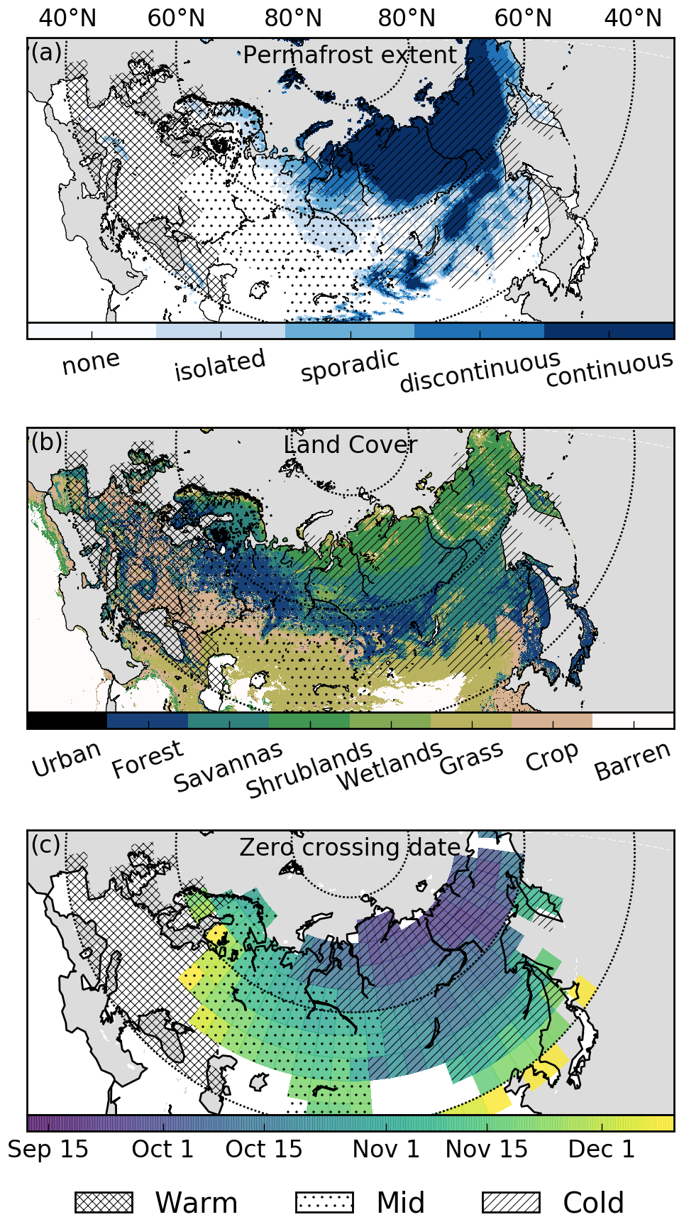
Figure 1(a) Permafrost extent over 2000–2016 (Obu et al., 2018, 2019). (b) MODIS International Geosphere Biosphere Programme (IGBP; MOD12C1 v6) land cover for urban areas, forest (tree cover > 60 % and height > 2 m), savanna (tree cover 10 %–60 % and height > 2 m), shrublands (woody perennials cover > 10 % and height < 2 m), grasslands, croplands, and barren land. (c) Zero-crossing date (date when the mean soil temperature drops below 0 ∘C) for the top 0.5 m of soil from the MERRA-2 Land dataset at 4∘ × 5∘ spatial resolution. Grid cells with no shading do not have a zero-crossing date. Three regions are shown by different hatching patterns. The “Warm” (cross hatching) region does not have a zero-crossing date, the “Mid” (dots) region has a zero-crossing date after 27 October, and the “Cold” (diagonal hatching) region has a zero-crossing date before 27 October. Note that some adjustments from these definitions are made so that the regions are contiguous. The Warm, Mid, and Cold regions have land areas of 5.66×10⁶ km2, 8.66×10⁶ km2, and 12.65×10⁶ km2, respectively.
We first examine the seasonality of net ecosystem exchange (NEE) constrained by atmospheric inversions of retrieved column-averaged dry-air mole fractions of CO2 () from the Orbiting Carbon Observatory 2 (OCO-2) (Crisp et al., 2017; Eldering et al., 2017) and by flask and in situ CO2 measurements (Sect. 2.2). Monthly NEE is obtained from version 9 of the OCO-2 Model Inter-comparison Project (v9 OCO-2 MIP) (Peiro et al., 2022). In addition, we perform a set of three higher-temporal-resolution inversions using the CAMS, TM5-4DVar, and CMS-Flux (Carbon Monitoring System Flux) inversion systems to examine sub-monthly variability in CO2 fluxes. We then decompose NEE into component fluxes to better understand the processes driving the seasonality of NEE. In particular, we decompose the data-driven NEE fluxes into net primary production (NPP) and heterotrophic respiration (Rh):
To do this, we use four data-driven gross primary production (GPP) products: FLUXCOM (Jung et al., 2020), FluxSat (Joiner and Yoshida, 2020), the Vegetation Photosynthesis Model (VPM; Zhang et al., 2017), and the Global OCO-2-based solar-induced chlorophyll fluorescence (SIF) product (GOSIF; Li and Xiao, 2019). These datasets use Moderate Resolution Imaging Spectroradiometer (MODIS) reflectances, OCO-2 solar-induced fluorescence, and reanalysis data to infer GPP and thus provide an ensemble of global estimates of GPP to inform its uncertainty. NPP is estimated from GPP using the monthly carbon use efficiency (CUE) from the TRENDY models (Sect. 2.4) using the following relationship:
We then combine the data-driven estimates of NEE and NPP to recover a data-driven seasonal cycle of Rh (Sect. 2.5).
This analysis is performed at two temporal resolutions. First, we leverage the large ensembles from TRENDY and the v9 OCO-2 MIP that provide fluxes at monthly temporal resolution (Sect. 3.1). However, because phenological changes can be significant on shorter timescales (e.g., weekly; Parazoo et al., 2018a), we perform a second analysis at 14 d temporal resolution using three inversion analyses that optimize weekly or 14 d NEE fluxes (Sect. 3.2). For these 14 d fluxes, we further examine mechanistic explanations for data–model differences in Rh using a range of models (Sect. 3.3). Finally, we discuss the results (Sect. 4) and summarize our conclusions (Sect. 5).
2.1 Environmental data and region definitions
We utilize MERRA-2 Land soil temperature data (Reichle et al., 2011, 2017; Gelaro et al., 2017) to define three large regions within Eurasia (Fig. 1). These data were downloaded from the Goddard Earth Sciences Data and Information Services Center at monthly temporal resolution and 4∘ × 5∘ spatial resolution (regridded from model horizontal resolution of ∼ 50 km). Three regions are defined based on the date at which the top 0.5 m of MERRA-2 Land soil temperature falls below 0 ∘C, referred to as the “zero-crossing date”, for a mean seasonal cycle averaged over 4 years (2015, 2016, 2018, and 2019). The “Cold” region has a zero-crossing date before 27 October, the “Mid” region has a zero-crossing date after 27 October, and the “Warm” region does not have a zero-crossing date. This date was chosen as a cutoff to create two similarly sized Mid and Cold regions. Some adjustments from these definitions are made so that the regions are contiguous. We aggregate the CO2 fluxes described below to these regions by (1) interpolating the Warm, Mid, and Cold regions from 4∘ × 5∘ spatial resolution to the grid of the CO2 flux datasets (both GPP and NEE) and (2) calculating the area-weighted net fluxes over the regions. We also obtain the downward shortwave flux from the MERRA-2 Land dataset.
Several datasets are also used for supplementary evaluation of the MERRA-2 Land soil temperature seasonality (Sect. S2 in the Supplement). For that analysis, we use ERA5-Land reanalysis soil temperature data (Muñoz Sabater, 2019), generated using Copernicus Climate Change Service Information 2020. We also examined monthly soil temperature from seven models from the Coupled Model Intercomparison Project Phase 6 (CMIP6) (Eyring et al., 2016) for the historical simulations and Shared Socioeconomic Pathway 585 (ssp585) simulations, which is the highest emission scenario. The CMIP6 simulations were included to compare with MERRA-2 simulated soil temperature over 2010–2019 and to examine possible trends in soil temperature under a high-emission scenario. The model runs are CanESM5 (r1i1p2f1), MIROC ES2L (r1i1p1f2), ACCESS EMS1 (r1i1p1f1), MRI ESM2 0 (historical r1i1p1f1, ssp585 r1i2p1f1), CNRM ESM2 1 (r1i1p1f2), E3SM 1 1 (r1i1p1f1), and UKESM1 0 LL (r4i1p1f2). These models were chosen because they participated in the Coupled Climate–Carbon Cycle Model Intercomparison (C4MIP) (Jones et al., 2016). Finally, we compare the MERRA-2 Land soil temperature to borehole soil temperature measurements over the period 1998–2020, which were downloaded from the Global Terrestrial Network for Permafrost (GTN-P) borehole database (http://gtnpdatabase.org/boreholes, last access: 9 November 2021).
2.2 Atmospheric flux inversions
The OCO-2 Model Inter-comparison Project (OCO-2 MIP) provides standardized experimental setups for assimilating atmospheric CO2 to estimate net biosphere exchange (NBE), defined as
where BB is biomass burning, across a range of inversion systems. The v9 OCO-2 MIP (Peiro et al., 2022) provides ensembles of nine inversion systems that assimilated a standardized set of in situ and flask CO2 measurements for one experiment (referred to as “IS”) and OCO-2 ACOS b9 land nadir and land glint retrievals for a second experiment (referred to as “LNLG”). We estimate NEE fluxes from v9 OCO-2 MIP NBE fluxes by subtracting biomass burning emission estimates from the Global Fire Emissions Database version 4 (GFED4.1s) (van der Werf et al., 2017). GFED4.1s provides estimates of biomass burning using MODIS burned area (Giglio et al., 2013), thermal anomalies, and surface reflectance observations (Randerson et al., 2012). Note that biomass burning is a relatively small contribution to NBE over the regions examined here during the study period (2015–2019) (Fig. S1 in the Supplement). The NEE fluxes produced by each ensemble member over northern Eurasia are shown in Fig. S2.
To examine variability in fluxes at the sub-monthly time step, we examine three other inversion NEE estimates that optimize sub-monthly NEE fluxes: TM5-4DVAR14d LNLGIS, CAMS14d LNLGIS, and CMS-Flux14d LNLGIS. These inversions assimilated both in situ and flask CO2 in addition to OCO-2 ACOS b10 land nadir and land glint retrievals. Note that the ACOS b10 retrievals are updated from the b9 retrievals employed in v9 OCO-2 MIP. The prior and posterior NEE fluxes produced by each ensemble member are shown in Fig. S3, and the inversion setups are described below.
TM5-4DVAR is a variational inversion framework based on the TM5 atmospheric tracer transport model (Meirink et al., 2008; Basu et al., 2013). The TM5-4DVAR14d LNLGIS inversion assimilated 10 s averages of OCO-2 ACOS b10 land nadir and land glint measurements concurrently with in situ measurements to optimize weekly NEE and ocean fluxes. The OCO-2 10 s averages were constructed analogous to the b9 10 s averages assimilated by models in v9 OCO-2 MIP (Peiro et al., 2022). The in situ measurements assimilated were updated from Peiro et al. (2022); specifically ObsPack NRT 5.0 was replaced by NRT 5.2. The flux inversion setup was identical to the setup of “TM5-4DVAR” in Peiro et al. (2022), except (i) the inversion was run from 1 June 2014 to 1 February 2021 (instead of 1 September 2014 to 1 June 2019 in Peiro et al., 2022), (ii) ECMWF ERA5 meteorology was used to drive the model instead of ERA Interim, (iii) a 1∘ × 1∘ transport grid over North America was nested inside the global 3∘ × 2∘ grid to take advantage of the higher in situ data density, and (iv) prior CO2 fluxes were constructed following Weir et al. (2021).
The CAMS14d LNLGIS inversion utilizes the CAMS greenhouse gases inversion system (Chevallier et al., 2005, 2010; Chevallier, 2013) and assimilates OCO-2 land nadir and land glint 10 s averages and in situ CO2 measurements concurrently. A variational system is employed to optimize daytime and nighttime NEE at 8 d temporal resolution on a 1.875∘ × 3.75∘ model grid. Tracer transport is performed using the Laboratoire de Météorologie Dynamique (LMDz) general circulation model version LMDz6A (Remaud et al., 2018). These data were downloaded from https://atmosphere.copernicus.eu/ (last access: 29 August 2022). Note that CAMS reports NBE – as explained earlier, we estimate NEE using GFED4.1s biomass burning emissions, as was done for the v9 OCO-2 MIP.
The CMS-Flux14d LNLGIS flux inversions are performed using the setup of Byrne et al. (2020b), which uses the CMS-Flux inversion system that has been developed under the NASA Carbon Monitoring System Flux project (https://cmsflux.jpl.nasa.gov, last access: 29 August 2022) (Henze et al., 2007; Liu et al., 2014). These flux inversions optimize 14 d NEE and ocean fluxes by assimilating OCO-2 ACOS b10 land nadir and land glint “buddy” super-obs concurrently with in situ and flask measurements from version 6.0 of the GlobalView plus package (Masarie et al., 2014; Schuldt et al., 2020). OCO-2 “buddy” super-obs are obtained by averaging individual soundings into super-obs at 0.5∘ × 0.5∘ spatial resolution (within the same orbit) with equal weighting following Liu et al. (2017). We assimilate surface-based in situ and flask measurements between 11:00 and 16:00 local time. These data were also pre-filtered to remove observations that were not well simulated by the model (based on a posteriori data–model χ2 mismatches greater than three for a preliminary flux inversion). For these inversions, ODIAC fossil fuel emissions (Oda and Maksyutov, 2011; Oda et al., 2018) and GFED4.1s biomass burning emissions (van der Werf et al., 2017), including small fires (Randerson et al., 2012), are prescribed but not optimized.
2.3 Dynamic global vegetation models (DGVMs)
We use CO2 flux estimates from an ensemble of 15 dynamic global vegetation models (DGVMs) from TRENDY v8 (Sitch et al., 2015). We utilize fluxes simulated by the CABLE-POP, CLASS-CTEM, CLM5.0, DLEM, ISAM, ISBA-CTRIP, JSBACH, JULES, LPJ, LPX-Bern, OCN, ORCHIDEE, ORCHIDEE-CNP, SDGVM, and VISIT DGVMs. We exclude LPJ-GUESS because monthly output on Rh was not available. We utilize monthly GPP, autotrophic respiration (Ra), and Rh fluxes from the “S3” experiment that employs time-varying CO2, climate, and land use forcing data. We further calculate NPP from the simulated GPP and Ra data () at the models' native resolution. The NEE, NPP, and Rh fluxes produced by each ensemble member are shown in Fig. S4 for the same 3-year period as the data-driven estimates (2015, 2016, and 2018).
We also utilize TRENDY v8 model output to estimate an ensemble of carbon use efficiency () from each DGVM. CUE can become negative during the winter and spring, when GPP is approximately zero but Ra is non-zero. However, we limit CUE values to a range between zero and one. These CUE estimates are then employed to estimate data-driven NPP estimates from the data-driven GPP data (see Sect. 2.4). Figure S5 shows the CUE estimates derived from the TRENDY v8 models.
2.4 GPP datasets and NPP estimates
We utilize four data-driven GPP estimates in this analysis: FluxSat, FLUXCOM, VPM, and GOSIF. These datasets differ in inputs and approach.
FluxSat Version 2 (Joiner and Yoshida, 2020) estimates GPP based on Nadir BRDF-Adjusted Reflectance (NBAR) from the MODIS MYD43D product (Schaaf et al., 2002). The GPP estimates are calibrated with the FLUXNET2015 GPP derived from eddy covariance flux measurements at Tier 1 sites (Pastorello et al., 2020).
FLUXCOM upscales CO2 fluxes from flux tower observations using a variety of machine learning methods and forcing datasets (Jung et al., 2020). We examine the ensemble mean of the nine remote sensing (RS) learning algorithms.
VPM is a light use efficiency model that estimates GPP globally using MODIS surface reflectances and NCEP Reanalysis-2 photosynthetically active radiation and temperature data (Xiao et al., 2004; Zhang et al., 2017). The native spatiotemporal resolution of the dataset is 500 m and 8 d. VPM has been shown to agree well with FLUXNET eddy covariance site-level data (Zhang et al., 2017) and with TROPOMI SIF at the global scale (Doughty et al., 2021).
The GOSIF GPP product estimates GPP based on OCO-2 SIF, MODIS EVI, and reanalysis data from MERRA-2 (Li and Xiao, 2019). To generate GPP estimates, first, 8 d globally gridded 0.05∘ × 0.05∘ SIF is estimated from the input data using machine learning algorithms. GOSIF GPP is then estimated from the GOSIF SIF estimates using eight SIF–GPP relationships with different forms (universal and biome-specific, with and without intercept). In this analysis we utilize the mean GPP estimate across the eight SIF–GPP estimates.
These four data-driven GPP estimates are shown in Fig. S6. For this analysis, we estimate NPP from these data using the CUE from the TRENDY models. We perform this calculation differently for the monthly analysis and biweekly analysis. For the monthly analysis, we calculate 60 NPP seasonal cycles for each possible combination of the four GPP and 15 CUE seasonal cycles. We then calculate the mean as our best estimate and interquartile range as a metric of uncertainty. For the biweekly analysis, we calculate the best estimate using the mean GPP and CUE seasonal cycles and calculate the uncertainty using the full range of GPP estimates and interquartile range of CUE estimates. This is done differently to match the NEE analysis, which leverages the larger ensemble from the v9 OCO-2 MIP to examine the mean and interquartile spread for the monthly analysis but employs the full range for the smaller biweekly ensemble of three models.
2.5 Data-driven Rh estimates
We calculate the seasonal cycle of Rh by combining the data-driven estimates of NPP and NEE using Eq. (1) (). We perform this calculation differently for the monthly analysis and biweekly analysis. For the monthly v9 OCO-2 MIP IS- and LNLG-based estimates, we calculate 540 Rh seasonal cycles by combining the 9 data-driven IS or LNLG NEE estimates with the 60 NPP estimates. We then take the mean and interquartile spread as the best estimate and uncertainty. For the biweekly analysis, we calculate the best estimate of Rh from the best (mean) estimates of NPP and NEE. We then specify the uncertainty to be the full range of Rh estimates calculated from the three biweekly NEE estimates and the NPP range.
2.6 Soil carbon decomposition model
We use the soil carbon decomposition model developed in Yi et al. (2015, 2020) to simulate the contribution of soil at different depths to total Rh and NEE fluxes. The soil decomposition model uses multiple litter and soil organic carbon (SOC) pools to characterize the progressive decomposition of fresh litter to more recalcitrant materials, which include three litterfall pools, three SOC pools with relatively fast turnover rates, and a deep SOC pool with slow turnover rates. The litterfall carbon inputs were first allocated to the three litterfall pools depending on the substrate quality of litterfall component and then transferred to the SOC pools through progressive decomposition. We then model the profile of the carbon pools through accounting for the vertical carbon transport (Yi et al., 2020). A constant diffusivity rate was assigned to permafrost (5.0 cm2 yr−1) and non-permafrost (2.0 cm2 yr−1) regions within the top 1 m soil and then linearly decreased to 0 at the 3 m b.s. (below surface) (Koven et al., 2013). The boundary conditions at the soil surface were set as the carbon input rate to the three surface litterfall pools. A zero-flux was assigned at the bottom of the soil carbon pool, which was set as 3 m. This accounts for the upper permafrost layer, while carbon in deeper layers (e.g., 3–10 m) is largely insulated from climate variability and ignored in this study. The decomposition rate (d−1) for each carbon pool was derived as the product of a theoretical maximum rate constant and dimensionless multipliers for soil temperature and liquid water content constraints (Yi et al., 2015). In this study, the decomposition was driven by the MERRA2 soil temperature data. For simplicity, the soil saturation was assumed as 1.0 when soil temperature is above 0 ∘C, while the maximum liquid soil water fraction was used for below freezing (Schaefer and Jafarov, 2016).
2.7 FLUXNET data and processing
We examine 15 high-latitude FLUXNET2015 sites to confirm the seasonality of carbon fluxes inferred from the atmospheric CO2 and remote sensing datasets. These sites are listed in Table S1. For this, we utilize monthly data with the quality flag greater than 0.75. We calculate NPP and Rh for each site from the NEE and GPP datasets by applying the CUE from the TRENDY DGVMs at the grid cell containing the FLUXNET site.
3.1 Differences between data-driven and DGVM carbon fluxes
We first examine the mean seasonal cycle of monthly NEE from the v9 OCO-2 MIP inversions and TRENDY v8 DGVMs over the three northern Eurasian regions (mean over 2015, 2016, and 2018; 2017 is excluded due to an OCO-2 data gap during August–September). The objective of this initial analysis is to identify the seasonal features of NEE over northern Eurasia and identify how the data-driven and simulated estimates differ. The spread among the TRENDY v8 models is large and encompasses the data-driven estimates (Fig. S4). Thus, to identify data–model differences, we focus on differences in the ensemble mean estimates and adopt the interquartile spread across v9 OCO-2 MIP and TRENDY to quantify uncertainty in this estimate.
Figure 2a–c show the NEE fluxes for the v9 OCO-2 MIP and TRENDY DGVMs for three regions over Eurasia. The two v9 OCO-2 MIP ensembles (IS and LNLG) generally show close agreement and coherent differences from the TRENDY models (and prior NEE estimates; Fig. S2). The largest differences between the IS and LNLG ensembles occur over the Cold region, where the IS ensemble suggests increased uptake during July and somewhat increased release during October. Still, the coherent differences between the data-driven fluxes (both IS and LNLG) relative to the TRENDY ensemble gives us increased confidence that these inversions are precisely capturing the seasonality of NEE. The comparatively good agreement between the IS and LNLG inversions (relative to TRENDY) also suggests that artifacts related to observational coverage (Byrne et al., 2017; Basu et al., 2018) and data and model biases (Schuh et al., 2019) do not strongly impact the results, although we note that both datasets have spatial and seasonal gaps over northern Eurasia (e.g., Figs. S7–S8) as discussed in Sect. 4.2. The accuracy of the v9 OCO-2 MIP fluxes is supported through an evaluation of the posterior CO2 fields against independent atmospheric CO2 measurements by Peiro et al. (2022), as well as a supplementary comparisons of the CMS-Flux14d inversions with aircraft data over Alaska (Sect. S1, Figs. S9–S10).
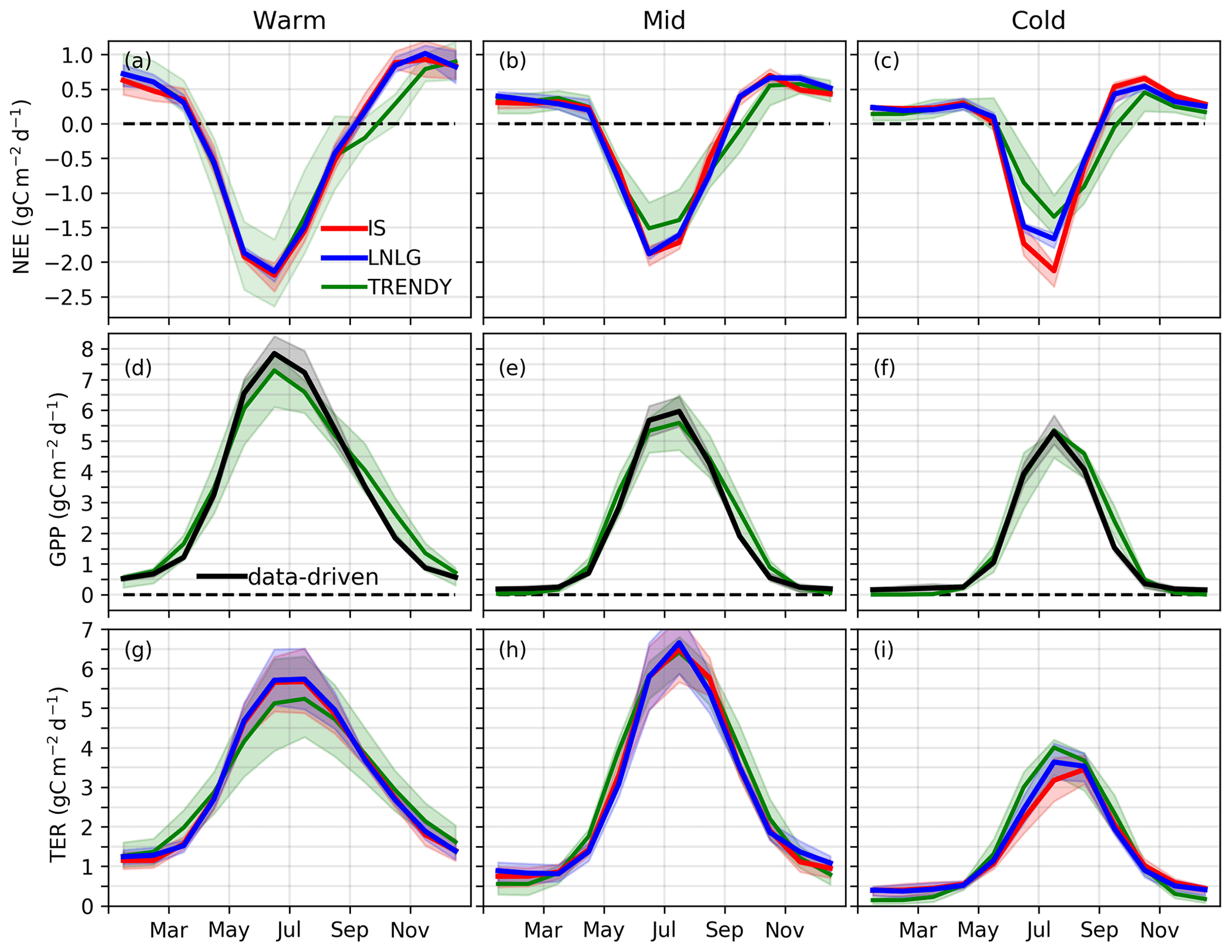
Figure 2Monthly carbon cycle fluxes (average of 2015, 2016, and 2018; 2017 is excluded due to an OCO-2 data gap). (a–c) Mean (solid line) and interquartile range (shaded area) of NEE for the ensemble of IS (red) and LNLG (blue) v9 OCO-2 MIP and for the TRENDY ensemble (green). (d–f) GPP for the TRENDY ensemble (green) and data-driven datasets (black). (g–i) TER simulated by the TRENDY ensemble (green) and calculated from combining the data-driven GPP with the IS (red) and LNLG (blue) v9 OCO-2 MIP NEE constraints.
Comparing the v9 OCO-2 MIP and TRENDY NEE estimates, good agreement is found for the Warm and Mid regions, while larger differences are found for the Cold region. In the Warm and Mid regions, systematic differences exceed the interquartile range during September–October, when the TRENDY models suggest a weaker efflux of CO2 to the atmosphere (0.30–0.51 g C m−2 d−1). The TRENDY models also tend to show weaker uptake by land during June–July in the Mid region (0.05–0.35 g C m−2 d−1). For the Cold region, the TRENDY models produce weaker carbon uptake during June–July (0.48–0.83 g C m−2 d−1) but stronger uptake (or reduced efflux) during August–October (0.31–0.36 g C m−2 d−1). This large amplitude of the NEE seasonal cycle contributes to the large seasonality in observed over eastern Eurasia (Jacobs et al., 2021).
To further investigate the causes of differences in NEE between the TRENDY and v9 OCO-2 MIP ensembles, we separately examine component primary productivity and respiration fluxes. For the most direct decomposition, we employ the data-driven GPP estimates to decompose NEE into GPP and terrestrial ecosystem respiration (TER) fluxes (Fig. 2). This comparison shows that the TRENDY ensemble mean GPP tends to overestimate the data-driven GPP during the autumn (September–November), largely explaining the mismatch in NEE during this season. For TER, we find good agreement for over the Warm region except for an underestimate of TER for the TRENDY ensemble mean during the summer (mirroring GPP). For the Mid region, agreement is found between the TRENDY and data-driven TER estimates throughout the growing season. For the Cold region, we find that the TRENDY ensemble mean suggested greater TER during May–August, which drives the mismatch found in NEE.
We next decompose NEE into component NPP and Rh fluxes. These estimates require an additional assumption about the CUE in comparison to the GPP/TER decomposition but also have the potential to provide more process understanding. As described in Sect. 2.4, we employ the monthly CUE estimates from the ensemble of TRENDY models. This both allows an “apples-to-apples” comparison with the TRENDY models as the CUE estimates are consistent between the data-driven and TRENDY estimates and allows us to propagate uncertainty in CUE from the ensemble spread. The data-driven NPP and TRENDY NPP are shown in Fig. 3d–f. The seasonality in NPP between the data-driven and TRENDY estimates show good agreement for all regions. In the Mid and Warm regions, the TRENDY model mean NPP tends to be lower than the data-driven estimates during June–July (0.26–0.37 g C m−2 d−1). However, the largest differences are for the Cold region, where the TRENDY ensemble mean shows increased NPP during August–September (0.38 g C m−2 d−1). This largely accounts for the lower NEE during August–September (86 %–95 %). Thus, despite previously reported deficiencies in model representation of photosynthesis over high latitudes (Rogers et al., 2017, 2019), we find that TRENDY NPP estimates largely capture the data-driven seasonality and do not drive NEE differences against the data-driven seasonal cycle.
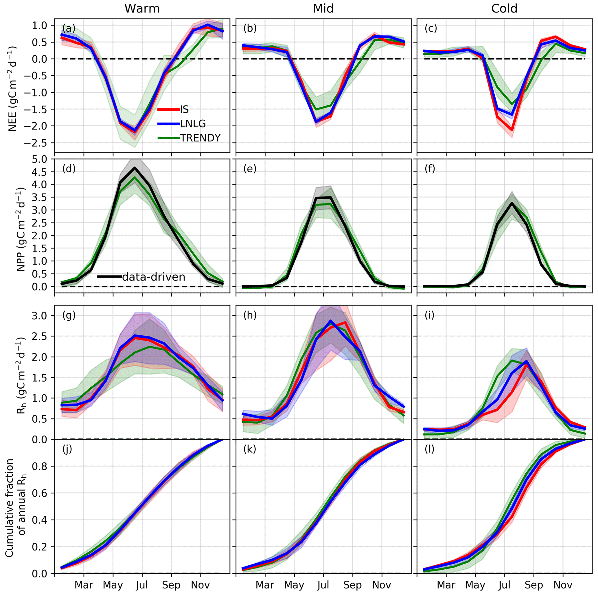
Figure 3Monthly carbon cycle fluxes (average of 2015, 2016, and 2018; 2017 is excluded due to an OCO-2 data gap). (a–c) Mean (solid line) and interquartile range (shaded area) of NEE for the ensemble of IS (red) and LNLG (blue) v9 OCO-2 MIP and for the TRENDY ensemble (green). (d–f) NPP for the TRENDY ensemble (green) and estimated from data-driven GPP (black). (g–i) Rh simulated by the TRENDY ensemble (green) and calculated from combining the data-driven NPP with the IS (red) and LNLG (blue) v9 OCO-2 MIP NEE constraints. (j–l) Cumulative fraction of Rh over the growing season.
Finally, we compare TRENDY Rh to data-driven Rh (Fig. 3g–i). In the Warm region, the TRENDY model mean Rh is lower than the data-driven estimates during May–September (0.21–0.26 g C m−2 d−1), but the seasonality is similar. In the Mid region, the data-driven and TRENDY Rh seasonal cycles show good agreement throughout the growing season. The largest differences between data-driven and TRENDY Rh seasonal cycles are found for the Cold region. The TRENDY model mean shows increased Rh during May–July (0.32–0.58 g C m−2 d−1) but show reduced Rh during the rest of the year (0.29–0.51 g C m−2 d−1). As a result, the seasonality of data-driven Rh is shifted later in the year relative to the TRENDY ensemble. This can be seen in the cumulative fraction of annual Rh, which quantifies the fraction of total Rh released as the season progresses (Fig. 3j–l). The percentage of total annual Rh released during May–July is 46 % for the TRENDY ensemble mean but 37 % (30 %) for the LNLG (IS) data-driven Rh ensemble mean.
We independently confirm a shift in the seasonality of data-driven Rh relative to TRENDY for 15 high-latitude FLUXNET sites (Fig. S11). Due to the sparsity of FLUXNET sites over northeastern Eurasia, we include sites outside of the “Cold” domain but that have early zero-crossing dates (estimated by a mean October air temperature less than 2 ∘C). The observed mean Rh peaks across these sites during September, in agreement with the data-driven Rh seasonality. In contrast, the TRENDY mean Rh peak occurs during July (consistent with the regional-scale analysis). This phase shift is also evident in the cumulative fraction of annual Rh, which shows that the percentage of total annual Rh released during May–July is 46 % for the TRENDY ensemble mean but 35 % for the FLUXNET-based ensemble mean.
Overall, these results indicate good agreement between the TRENDY ensemble and data-driven estimates for the Warm and Mid regions but show marked differences over the Cold region. In particular, we find that the data-driven estimates suggest a seasonal redistribution of Rh with a reduction during May–July but an increase for the remainder of the year. Further, these results show that differences in Rh largely account for the differences between the data-driven and TRENDY NEE fluxes over the Cold region, except in August–September when NPP differences are large. In the remaining sections, we will characterize the data-driven seasonal cycle of NEE, NPP, and Rh at a higher (biweekly) temporal resolution and investigate mechanistic explanations for the data–model differences found over the Cold region.
3.2 Data-driven biweekly CO2 fluxes
We now investigate the data-driven seasonal cycle of NEE, NPP, and Rh with biweekly (14 d) temporal resolution. This higher resolution better resolves temporal changes in CO2 fluxes throughout the growing season, particularly during the shoulder seasons, when week-to-week changes in CO2 fluxes are large (Parazoo et al., 2018a). For this analysis, we utilize a set of three flux inversions that assimilate both in situ and OCO-2 land nadir and glint data (ACOS v10) to estimate sub-monthly CO2 fluxes (TM5-4DVAR14d, CAMS14d, and CMS-Flux14d; individual model fluxes shown in Fig. S3). These inversions give similar NEE seasonality to the v9 OCO-2 MIP monthly fluxes (e.g., Fig. S9) and have seasonality similar to the v9 OCO-2 MIP LNLG inversions for the Cold region. For NPP, we utilize the same datasets as Sect. 3.1 but at 14 d temporal resolution. We examine the ensemble means for a best estimate and take the full range of model estimates as an illustration of the uncertainty.
Figure 4 shows the 4-year-mean (2015, 2016, 2018, and 2019; 2017 is excluded due to an OCO-2 data gap in summer) seasonal cycle of NEE, NPP, and Rh for the three regions of Eurasia. NEE largely tracks the inverted seasonality of NPP, although peak NPP is slightly delayed relative to peak drawdown in NEE (by 0–2 weeks). Both NEE and NPP generally follow the seasonal cycle of insolation but are somewhat delayed in the Mid and Cold regions likely due to temperature limitation (Liu et al., 2020). Peak Rh is found to be delayed relative to peak NPP by 0–8 weeks. For the Warm and Mid regions, Rh follows the seasonal cycle of surface temperature, with 48 % and 51 % of the annual total Rh occurring after the peak in surface temperature, respectively. In contrast, the Cold region shows a substantial delay relative to surface temperature, with 63 % of the total Rh occurring after the peak in surface temperature. The mean Rh seasonal cycle is also found to have a double peak in this Cold region: a smaller peak of 0.77 g C m−2 d−1 occurs during late May followed by a larger peak of 1.70 g C m−2 d−1 at the beginning of September. This May peak roughly aligns with the spring thaw and positive zero-crossing at the beginning of May. A potential mechanistic explanation for a spring pulse of Rh could be due to thawing soils that release CO2 that had been trapped within subsurface soil layers over the winter (see Sect. 4). Another plausible mechanism could be the timing of snowmelt, which may insulate the soil over winter (Yu et al., 2016). However, the signal from this first peak is small relative to the uncertainties.
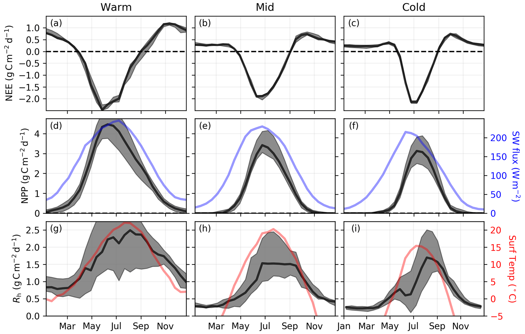
Figure 4Data-driven 4-year-mean (2015, 2016, 2018, and 2019) 14 d NEE, NPP, and Rh. (a–c) Mean and ensemble spread of NEE for the CMS-Flux14d, TM4-4DVar14d, and CAMS14d flux inversions. (d–f) Mean and ensemble spread for the data-driven NPP. MERRA-2 Land net downward shortwave flux over land is shown in blue. (g–i) Ensemble estimate of estimated from the three NEE and NPP estimates. MERRA-2 Land surface temperature is shown in red.
3.3 Mechanistic drivers of late-season Rh
Data-driven Rh for the Cold region indicates a delayed peak relative to surface temperature and the TRENDY model mean. Here we examine possible mechanistic explanations for this late season peak in Rh using models. We investigate two factors that could potentially contribute to the delay in Rh. (1) The first factor is seasonal variations in the labile carbon pool. Leaf and fine root litter carbon pools tend to increase over the growing season as carbon is sequestered through photosynthesis (Randerson et al., 1996). Thus, increased substrate availability in the autumn relative to the spring will act to shift the seasonal cycle of Rh later in the year. (2) The second factor is Rh from subsurface soil layers that have a delayed seasonal cycle driven by a lag in soil temperature. Heating and cooling at the surface slowly diffuses through the soil column resulting in a lagged seasonal cycle of temperature with depth (Parazoo et al., 2018b). Figure 5a–c show the seasonal cycle in soil temperature from the MERRA-2 Land dataset. The phase shift in soil temperature seasonality with depth can be up to several months and is largest for the colder regions. Note that we verify the fidelity of the MERRA-2 Land soil temperature against borehole measurements and against simulated soil temperature from ERA-5 reanalysis and the CMIP6 models (see Sect. S2, Figs. S12–S13).

Figure 5Impact of temporal and vertical variations in carbon pools on Rh. (a–c) MERRA-2 Land soil temperature over five intervals for the (a) Warm, (b) Mid, and (c) Cold regions. (d–e) Mean and range in inferred 14 d Rh with fits for single-layer Rh models that employ (navy dash) Tsurf dependence and no seasonal variations in the carbon pool, (cyan dash) T1 m dependence and no seasonal variations in the carbon pool, and (magenta dash) Tsurf dependence and seasonal variations in the carbon pool. (g–i, top) Normalized seasonal cycle of Rh simulated by the soil decomposition model (Sect. 2.6). The different lines show different model simulations: D300 cm employs a dynamic carbon pool over 0–300 cm depth, C300 cm employs a constant carbon pool over 0–300 cm depth, and D10 cm employs a dynamic carbon pool over 0–10 cm depth. (g–i, bottom) Differences in simulated Rh between experiments.
To test the impact of these factors, we consider a single layer model that represents Rh using a exponential relationship with temperature:
where α represents the labile carbon pool size, β is a constant, and T is the temperature of the carbon pool. To investigate the impact of seasonal and vertical variations in labile carbon, we consider three cases:
-
: the carbon pool is constant in time (αc), and the surface temperature (Tsurf) drives Rh;
-
: the carbon pool is constant in time (αc), and the average top meter soil temperature (T1 m) drives Rh;
-
: the carbon pool is dynamic in time (αt=f(t), described in the Appendix), and the Tsurf drives Rh. We assume seasonal variations in the carbon pool are within ± 15 % of the mean (γ=0.15, Fig. S14 shows the seasonal variation in the labile carbon pool).
Figure 5d–f show linear regressions for each one-layer model against the mean biweekly estimate of Rh. In each case, the parameters α and β are optimized (note linear regressions are performed on ). Statistics on the model fits are provided in Table 1. For the Warm region, all models are able to fit the data well (R2= 0.89–0.93, SE=0.051–0.067 g C m−2 d−1). Similarly, all models are able to largely capture the seasonal cycle in the Mid region (R2= 0.84–0.94), although Rh(αc,T1 m) appears to better capture the shoulder seasons and gives a smaller standard error (SE= 0.046 g C m−2 d−1) than the other models (SE=0.074–0.091 g C m−2 d−1). The models diverge the most for the Cold region. Rh(αc,Tsurf) gives the poorest performance (R2=0.66, SE=0.16 g C m−2 d−1), as the driving temperature data peak too early to capture the seasonality of Rh. Rh(αt,Tsurf) performs somewhat better, as the peak in model Rh is delayed relative to surface temperature (R2=0.77, SE=0.13 g C m−2 d−1). Still, Rh(αc,T1 m) performs the best (R2=0.88, SE=0.08 g C m−2 d−1) and best captures the delayed Rh seasonality relative to surface temperature.
Table 1Parameters (α,β) for one-layer model fits and statistics (slope, intercept, R2, standard error – SE) on the data–model mismatch of these fits.

To further confirm that Rh(αc,T1 m) best captures the seasonality of Rh, we fit these same models to seasonal FLUXNET Rh averaged over cold sites. This is a rather rough comparison as we drive the models with soil temperatures averaged over the Cold region rather than site specific datasets (due to absence of soil temperature data). Figure S15 shows the resulting fits, and Table S2 gives the statistics of the fits. We find that Rh(αc,T1 m) performs best (R2=0.96, SE=0.08 g C m−2 d−1), while Rh(αt,Tsurf) performs second best (R2=0.85, SE=0.19 g C m−2 d−1), and Rh(αc,Tsurf) gives the poorest performance (R2=0.75, SE=0.25 g C m−2 d−1), consistent with the regional-scale data-driven analysis.
This analysis demonstrates that the seasonality of Rh in the Warm and Mid regions is reasonably explained by seasonal variations in Tsurf but that inclusion of seasonal variations in the labile carbon pool and the impact of soil temperature with depth still improve the seasonal fit. However, for the Cold region, the seasonality of Rh is not well captured by Tsurf, and additional factors, particularly the impact soil temperature with depth, are required to explain the delayed seasonality of Rh over the Cold region.
We further investigate these mechanisms using a soil carbon decomposition model that can simulate seasonal and vertical variations in carbon pools (Sect. 2.6). This allows for a prognostic simulation of mechanisms driving the seasonality, in contrast to the diagnostic one-layer models. Three experiments are examined that simulate Rh: (1) down to a depth of 300 cm using a constant carbon pool (C300 cm), (2) within the top 10 cm of soil using a dynamic carbon pool (D10 cm), and (3) to a depth of 300 cm using a dynamic carbon pool (D300 cm due to dynamic litterfall inputs and Rh outputs). We compare these seasonal cycles after normalizing by the annual total Rh. Figure 5g–i show that incorporating seasonal and vertical variations in the carbon pool results in a phase shift in Rh to later in the year, consistent with the one-layer model results. The simulated impact of these factors is found to be quite small possibly due to underestimation of the impact of seasonal and vertical variations in the carbon pools on Rh in the model. Still, these model simulations can inform the Rh tendencies of these carbon pool variations. Comparing the regions, the impact of seasonal variations in the labile carbon pool are quite similar, with reduced Rh in the summer and increased Rh during the autumn relative to a constant carbon pool. In contrast, the impact of vertically resolved Rh shows differences between the regions, with a small impact for the Warm region but a comparatively large impact for the Cold region. The larger impact over the Cold region is likely due to larger carbon pools at depth (Fig. S17), with a possible contribution from regional differences in the thermal gradient with depth (Fig. 5). Similarly, we find that the fractional contribution of subsurface soils to total Rh has larger seasonal variation over the Cold region (Fig. S18). Thus, these results support a substantial contribution of subsurface soil Rh and suggest that an underestimation of this quantity by the DGVMs could explain the data–model differences.
4.1 Implications
Over the cold northeastern region of Eurasia, our data-driven Rh seasonal cycle allocates 64 %–70 % of annual CO2 emissions to outside of the summer (August–April) compared to only 52 % of annual Rh emissions allocated by the TRENDY DVGMs to this period. The reason that the TRENDY models do not capture this seasonality is unclear. A plausible explanation is that the TRENDY models do not capture the contribution of subsurface layers to Rh, especially during the zero-curtain period. This is clearly the case for the subset of TRENDY models that drive Rh with air temperature. However, it is unclear if this is an important factor for models with more sophisticated soil modules. Surprisingly, a preliminary analysis did not find a relationship between model complexity and agreement with the data-driven estimate. The drivers of differences from the data-driven estimate may differ between models and be impacted by the interplay of litterfall phenology, Rh formulation (Peylin et al., 2005), and number of soil layers, among other factors. Some potential areas of focus for improving models may be gleaned from recent studies. Seiler et al. (2022) suggest that the TRENDY models may systematically underestimate soil organic carbon at high latitudes, which could contribute to an underestimate of subsurface Rh across the models. Endsley et al. (2022) found a similarly phased bias in simulated Rh by the Terrestrial Carbon Flux (TCF) model against flux tower Rh to that reported here. They show that this bias could be largely mitigated by adding seasonally varying litterfall phenology, an O2 diffusion limitation on Rh, and a vertically resolved soil decomposition model, suggesting these may be foci for model improvements.
Differences between the data-driven and TRENDY Rh seasonal cycles suggest that DGVMs may be deficient in simulating the response of permafrost-rich ecosystems to climate change, particularly in terms of subsurface Rh. Improving DGVM skill in these ecosystems is critical given the rapid northern high-latitude warming and lengthening of the zero-curtain period (Euskirchen et al., 2017; Parazoo et al., 2018b; Chen et al., 2021). The rapid changes in northern Eurasia are illustrated in Fig. 6, which shows the number of months per year that soil temperatures are greater than 0 ∘C as simulated by a set of CMIP6 models. Soils in the permafrost-rich Cold region are undergoing the most dramatic lengthening of the unfrozen period, particularly at depth (50–200 cm). Under scenario ssp585 (highest emission scenario), these soils are predicted to go from ∼5 months per year with a monthly mean soil temperature above 0 ∘C during the 20th century to ∼ 11 months per year by 2100. The impact is largest for the Cold region at depth because of the reduced seasonality relative to the surface such that a warming of ∼ 7 ∘C shifts nearly the entire seasonal cycle above 0 ∘C at a depth of 50–200 cm (Fig. S19). Such warming would drive the widespread formation of talik, a subsurface layer of perennial thawed soil (Parazoo et al., 2018b), and further enhance Rh at depth.

Figure 6Number of months per year with monthly mean soil temperatures above 0 ∘C at depths of 0–10 cm (red), 10–50 cm (green), and 50–200 cm (blue) simulated by seven CMIP6 models under ssp585 for the (a) Warm, (b) Mid, and (c) Cold regions. The solid lines show the model mean, and shading shows ± 1 SD.
Rh from sub-surface layers may already be increasing substantially in permafrost regions. Examining the 41-year record of CO2 at Barrow tower, Commane et al. (2017) find that early cold season NEE efflux (October–December) has increased 73.4 % ± 10.8 % over the 1975–2015 period. The standard CAMS IS inversion product similarly suggests an increase in the September–October NEE efflux of ∼ 80 % over Siberia for the 2013–2017 period relative to the 1980–1984 period (see Fig. S20 of Lin et al., 2020). In agreement, Hu et al. (2021) identified a strong increase (∼ 10 %) in August–October Rh over the North America Arctic–boreal region between 1979–1988 and 2010–2019 based on measurements of atmospheric CO2 and carbonyl sulfide. These inferred changes in Rh may in part be related to warming-induced changes in the seasonality of GPP (Liu et al., 2020; Kwon et al., 2021), but more research is needed to determine the impact of these different drivers.
4.2 Limitations
Atmospheric CO2 measurements are relatively sparse over northern Eurasia (Byrne et al., 2017). In situ and flask CO2 measurements are spatially sparse over Mid and Cold regions (Fig. S8), with only a handful of sites assimilated over Russia as part of Japan–Russia Siberian Tall Tower Inland Observation Network (JR-STATION) of nine tower sites (Sasakawa et al., 2010, 2013). The OCO-2 coverage is seasonally variable (Fig. S7). Due to the fact that retrievals are performed on reflected sunlight, the coverage across Eurasia is quite good during the growing season (May–September). However, low signal and the inability to perform retrievals over snow limit the data coverage during the shoulder seasons and winter, resulting in few retrievals across the Mid and Cold regions during November–February. Ongoing research to both improve quality control filtering at high latitudes (Jacobs et al., 2020; Mendonca et al., 2021) and retrieve over snow and ice surfaces (Mikkonen et al., 2021) may reduce these data gaps in the future. Despite this sparsity of measurements, we find that the LNLG and IS flux inversions show consistent differences from the TRENDY and prior fluxes. Furthermore, these data show good agreement with withheld in situ data (Peiro et al., 2022) and independent aircraft measurements over Alaska (Fig. S10). Thus, we believe the results presented here to be robust despite data gaps. Still, this sparsity of data leads to some limitations. There are few sources of independent CO2 measurements over the Mid and Cold regions to evaluate the inversion posterior CO2 fields. Independent measurements (possibly aircraft campaigns) would provide a valuable additional data set for validation. Similarly, increasing the number of year-round eddy-covariance sites across the Mid and Cold regions would provide a valuable independent dataset to compare against flux inversion estimated NEE. For example, Byrne et al. (2020a) were able to confirm top-down estimates of east–west differences in NEE interannual variability across North America against the dense network of eddy-covariance sites.
We also note that there are challenges in estimating data-driven GPP during the shoulder season due to reduced reflected radiance and snow cover, which impacts the spectral features of the vegetation canopy. Poor quality data, such as snowy and noisy samples, contribute to uncertainty in the timing of shoulder seasons (Wang et al., 2017; Zhang, 2015). In this analysis, we attempted to mitigate this issue through the use of an ensemble of data-driven GPP estimates, but we acknowledge that remaining biases may be present.
Furthermore, the partitioning of NEE into NPP and Rh could be biased if CUE estimates were seasonally biased. We employed TRENDY model CUE to translate data-driven constraints on NEE and GPP into estimates of NPP and Rh. Thus, systematic errors across the TRENDY ensemble in CUE could impact conclusions about the relative contributions of errors in NPP and Rh. A potential source of bias in CUE could be due to an underestimate of the impact of inhibition of leaf respiration by light (Wehr et al., 2016; Byrne et al., 2018; Keenan et al., 2019; Oikawa et al., 2017). This would result in greater CUE and NPP during June–July relative to the rest of the year, shifting the inferred Rh seasonal cycle earlier, with Rh increased during June–July but decreased elsewhere (Byrne et al., 2018). However, the magnitude of this impact on the ecosystem scale is uncertain, making accounting for this phenomenon challenging. Recently, Endsley et al. (2022) found that the inhibition of leaf respiration by light has a relatively modest impact on the seasonality of NPP and Rh, suggesting that the results presented here are robust.
There are also remaining challenges in relating the inferred fluxes to underlying processes. Space-based flux constraints do not discriminate between biological and physical processes driving carbon cycle fluxes. It is currently unclear whether the substantial cold season CO2 effluxes across permafrost regions are driven primarily by biological activity or physical processes (Natali et al., 2019; Arndt et al., 2020; Raz-Yaseef et al., 2017). Yet, isolating the primary driver of these fluxes is critical for inferring the sensitivity of Rh to climate change. If the cold season Rh comes from the metabolism of old permafrost carbon, then 14CO2 measurements could help differentiate biological from physical CO2 production.
Space-based and in situ atmospheric CO2 measurements revealed strong summer uptake and early cold season release of CO2 over the cold northeastern Eurasia region, implying a late summer peak in Rh with substantial early cold season respiration. Based on model simulations of Rh, we suggested that this seasonality is driven by a large contribution of subsurface soils to the total Rh. These results are consistent with site-level observations identifying substantial CO2 release in permafrost regions outside the growing season (Natali et al., 2019) and, in particular, reported spikes in early cold season respiration associated with the zero-curtain period in Arctic ecosystems (Commane et al., 2017; Jeong et al., 2018).
The data-driven seasonality of Rh over the Cold region was generally not captured by the TRENDY DGVMs, which showed greater Rh during May–July and lower Rh during the rest of the year. The underlying cause of this discrepancy is unclear but may be linked to an underestimate of the contribution of sub-surface soils to total Rh. Given the rapid warming of permafrost soils (Euskirchen et al., 2017; Chen et al., 2021), talik formation (Parazoo et al., 2018b), and increasing early cold season CO2 effluxes (Commane et al., 2017; Lin et al., 2020; Hu et al., 2021), improving DGVM simulations in permafrost regions should be a focus of future studies.
This analysis demonstrates the utility of space-based observations for studying carbon cycle dynamics at high latitudes, where in situ measurements are sparse. Although currently limited by a short observing record (2014–present), the estimates of NEE inferred from the OCO-2 retrievals suggest that these data will provide a powerful tool for detecting change in seasonal cycle of NEE across northern Eurasia.
We estimate seasonal variations in labile carbon by estimating a litterfall flux of carbon. Litterfall seasonality is assumed to follow the same pattern as Randerson et al. (1996) (Fig. S14). We assume that the labile carbon pool is in steady state on annual timescales such that the annual total literfall is equal to the annual total Rh:
where t is the day of the year, and fNPP is the fraction of annual total NPP that is converted to litterfall. The seasonal variation in the labile carbon pool (ΔCpool) is defined as the difference in flux between litterfall and Rh:
Finally, we assume a fractional variation in the total carbon pool amount, γ, and calculate α(t):
where α0 is the mean carbon pool size and is optimized in the regression in Sect. 3.3.
TRENDY v8 gridded data were accessed by contacting Stephen Sitch following the TRENDY data policy described on their website: https://sites.exeter.ac.uk/trendy (Sitch et al., 2022). v9 OCO-2 MIP fluxes were downloaded from https://gml.noaa.gov/ccgg/OCO2_v9mip/ (Crowell et al., 2022). GFED data were downloaded from https://www.globalfiredata.org/ (Randerson et al., 2022). We downloaded version 10 of the ACOS OCO-2 lite files from the GES DISC (https://doi.org/10.5067/W8QGIYNKS3JC, OCO-2 et al., 2018). OCO-2 data were produced by the OCO-2 project at the Jet Propulsion Laboratory, California Institute of Technology, and obtained from the OCO-2 data archive maintained at the NASA Goddard Earth Science Data and Information Services Center. FluxSat data were downloaded from https://avdc.gsfc.nasa.gov/pub/tmp/FluxSat_GPP/ (Joiner, 2022). The GOSIF data product (Li and Xiao, 2019) is available at http://data.globalecology.unh.edu/, (Li and Xiao, 2019). ERA5-Land data are obtained from the Climate Data Store (https://doi.org/10.24381/cds.68d2bb30, Muñoz Sabater, 2019).
The supplement related to this article is available online at: https://doi.org/10.5194/bg-19-4779-2022-supplement.
BB, JL, YY, AC, KWB, NCP, DC, and CEM conceived of the study. BB, JL, YY, AC, and SB designed the experiments. YY performed the soil carbon decomposition model runs. BB, SB, and FC performed inversions for this study. BB, RC, and RD performed analysis of GPP data. XL and JX created GOSIF data. SS, BG, and PCM performed TRENDY simulations. BB created the figures and prepared the manuscript with contributions from all co-authors.
The contact author has declared that none of the authors has any competing interests.
Publisher’s note: Copernicus Publications remains neutral with regard to jurisdictional claims in published maps and institutional affiliations.
Brendan Byrne and Junjie Liu were supported by the NASA OCO2/3 science team program NNH17ZDA001N‐OCO2. Abhishek Chatterjee, Brendan Byrne, Junjie Liu, and Sourish Basu were also supported by the NASA OCO Science Team Grant #80NSSC21K1068. Charles E. Miller was supported by NASA's Arctic Boreal Vulnerability Experiment (ABoVE) under NNH18ZDA001N‐TE. Jingfeng Xiao was supported by the National Science Foundation (NSF) (Macrosystem Biology & NEON-Enabled Science program: DEB-2017870). Matthew S. Johnson acknowledges the internal funding from NASA's Earth Science Research and Analysis Program. Sajeev Philip acknowledges financial support of the NASA Academic Mission Services by Universities Space Research Association at NASA Ames Research Center. Frédéric Chevallier was funded by the Copernicus Atmosphere Monitoring Service, implemented by the European Centre for Medium-Range Weather Forecasts on behalf of the European Commission (grant no. CAMS73). The research carried out at the Jet Propulsion Laboratory, California Institute of Technology, was under a contract with the National Aeronautics and Space Administration. Resources supporting this work were provided by the NASA High‐End Computing (HEC) program through the NASA Advanced Supercomputing (NAS) Division at Ames Research Center. Frédéric Chevallier was granted access to the HPC resources of TGCC under the allocation A0110102201 made by GENCI. The ODIAC project is supported by Greenhouse Gas Observing SATellite (GOSAT) project, National Institute for Environmental Studies (NIES), Japan.
This research has been supported by the National Aeronautics and Space Administration (grant nos. 80NSSC21K1068, NNH17ZDA001N-OCO2, and NNH18ZDA001N-TE).
This paper was edited by David Bowling and reviewed by Ashley Ballantyne and one anonymous referee.
Arndt, K. A., Lipson, D. A., Hashemi, J., Oechel, W. C., and Zona, D.: Snow melt stimulates ecosystem respiration in Arctic ecosystems, Global Change Biol., 26, 5042–5051, 2020. a, b, c
Bastos, A., Ciais, P., Chevallier, F., Rödenbeck, C., Ballantyne, A. P., Maignan, F., Yin, Y., Fernández-Martínez, M., Friedlingstein, P., Peñuelas, J., Piao, S. L., Sitch, S., Smith, W. K., Wang, X., Zhu, Z., Haverd, V., Kato, E., Jain, A. K., Lienert, S., Lombardozzi, D., Nabel, J. E. M. S., Peylin, P., Poulter, B., and Zhu, D.: Contrasting effects of CO2 fertilization, land-use change and warming on seasonal amplitude of Northern Hemisphere CO2 exchange, Atmos. Chem. Phys., 19, 12361–12375, https://doi.org/10.5194/acp-19-12361-2019, 2019. a
Basu, S., Guerlet, S., Butz, A., Houweling, S., Hasekamp, O., Aben, I., Krummel, P., Steele, P., Langenfelds, R., Torn, M., Biraud, S., Stephens, B., Andrews, A., and Worthy, D.: Global CO2 fluxes estimated from GOSAT retrievals of total column CO2, Atmos. Chem. Phys., 13, 8695–8717, https://doi.org/10.5194/acp-13-8695-2013, 2013. a
Basu, S., Baker, D. F., Chevallier, F., Patra, P. K., Liu, J., and Miller, J. B.: The impact of transport model differences on CO2 surface flux estimates from OCO-2 retrievals of column average CO2, Atmos. Chem. Phys., 18, 7189–7215, https://doi.org/10.5194/acp-18-7189-2018, 2018. a
Bing, H., He, P., and Zhang, Y.: Cyclic freeze–thaw as a mechanism for water and salt migration in soil, Environ. Earth Sci., 74, 675–681, 2015. a
Björkman, M. P., Morgner, E., Cooper, E. J., Elberling, B., Klemedtsson, L., and Björk, R. G.: Winter carbon dioxide effluxes from Arctic ecosystems: An overview and comparison of methodologies, Global Biogeochem. Cy., 24, GB3010, https://doi.org/10.1029/2009GB003667, 2010. a
Byrne, B., Jones, D. B. A., Strong, K., Zeng, Z.-C., Deng, F., and Liu, J.: Sensitivity of CO2 Surface Flux Constraints to Observational Coverage, J. Geophys. Res.-Atmos, 112, 6672–6694, https://doi.org/10.1002/2016JD026164, 2017. a, b
Byrne, B., Wunch, D., Jones, D., Strong, K., Deng, F., Baker, I., Köhler, P., Frankenberg, C., Joiner, J., Arora, V. K., Badawy, B., Harper, A. B., Warneke, T., Petri, C., Kivi, R., and Roehl, C. M.: Evaluating GPP and Respiration Estimates Over Northern Midlatitude Ecosystems Using Solar-Induced Fluorescence and Atmospheric CO2 Measurements, J. Geophys. Res.-Biogeo., 123, 2976–2997, 2018. a, b
Byrne, B., Liu, J., Bloom, A. A., Bowman, K. W., Butterfield, Z., Joiner, J., Keenan, T. F., Keppel-Aleks, G., Parazoo, N. C., and Yin, Y.: Contrasting regional carbon cycle responses to seasonal climate anomalies across the east-west divide of temperate North America, Global Biogeochem. Cy., 34, e2020GB006598, https://doi.org/10.1029/2020GB006598, 2020a. a
Byrne, B., Liu, J., Lee, M., Baker, I. T., Bowman, K. W., Deutscher, N. M., Feist, D. G., Griffith, D. W., Iraci, L. T., Kiel, M., Kimball, J., Miller, C. E., Morino, I., Parazoo, N. C., Petri, C., Roehl, C. M., Sha, M., Strong, K., Velazco, V. A., Wennberg, P. O., and Wunch, D.: Improved constraints on northern extratropical CO2 fluxes obtained by combining surface-based and space-based atmospheric CO2 measurements, J. Geophys. Res.-Atmos., 125, e2019JD032029, https://doi.org/10.1029/2019JD032029, 2020b. a
Chen, L., Aalto, J., and Luoto, M.: Significant shallow–depth soil warming over Russia during the past 40 years, Global Planet. Change, 197, 103394, https://doi.org/10.1016/j.gloplacha.2020.103394, 2021. a, b
Chevallier, F.: On the parallelization of atmospheric inversions of CO2 surface fluxes within a variational framework, Geosci. Model Dev., 6, 783–790, https://doi.org/10.5194/gmd-6-783-2013, 2013. a
Chevallier, F., Fisher, M., Peylin, P., Serrar, S., Bousquet, P., Bréon, F.-M., Chédin, A., and Ciais, P.: Inferring CO2 sources and sinks from satellite observations: Method and application to TOVS data, J. Geophys. Res.-Atmos., 110, D24309, https://doi.org/10.1029/2005JD006390, 2005. a
Chevallier, F., Ciais, P., Conway, T. J., Aalto, T., Anderson, B. E., Bousquet, P., Brunke, E. G., Ciattaglia, L., Esaki, Y., Fröhlich, M., Gomez, A., Gomez‐Pelaez, A. J., Haszpra, L., Krummel, P. B., Langenfelds, R. L., Leuenberger, M., Machida, T., Maignan, F., Matsueda, H., Morguí, J. A., Mukai, H., Nakazawa, T., Peylin, P., Ramonet, M., Rivier, L., Sawa, Y., Schmidt, M., Steele, L. P., Vay, S. A., Vermeulen, A. T., Wofsy, S., and Worthy, D.: CO2 surface fluxes at grid point scale estimated from a global 21 year reanalysis of atmospheric measurements, J. Geophys. Res., 115, D21307, https://doi.org/10.1029/2010JD013887, 2010. a
Commane, R., Lindaas, J., Benmergui, J., Luus, K. A., Chang, R. Y.-W., Daube, B. C., Euskirchen, E. S., Henderson, J. M., Karion, A., Miller, J. B., Miller, S. M., Parazoo, N. C., Randerson, J. T., Sweeney, C., Tans, P., Thoning, K., Veraverbeke, S., Miller, C. E., and Wofsy, S. C.: Carbon dioxide sources from Alaska driven by increasing early winter respiration from Arctic tundra, P. Natl. Acad. Sci. USA, 114, 5361–5366, https://doi.org/10.1073/pnas.1618567114, 2017. a, b, c, d, e, f
Crisp, D., Pollock, H. R., Rosenberg, R., Chapsky, L., Lee, R. A. M., Oyafuso, F. A., Frankenberg, C., O'Dell, C. W., Bruegge, C. J., Doran, G. B., Eldering, A., Fisher, B. M., Fu, D., Gunson, M. R., Mandrake, L., Osterman, G. B., Schwandner, F. M., Sun, K., Taylor, T. E., Wennberg, P. O., and Wunch, D.: The on-orbit performance of the Orbiting Carbon Observatory-2 (OCO-2) instrument and its radiometrically calibrated products, Atmos. Meas. Tech., 10, 59–81, https://doi.org/10.5194/amt-10-59-2017, 2017. a
Crowell, S., Schuh, A., Baker, D. F., Jacobson, A. R., Chevallier, F., Liu, J., Deng, F., Weir, B., Basu, S., Johnson, M. S., and Philip, S.: v9 Orbiting Carbon Observatory-2 model intercomparison project, https://gml.noaa.gov/ccgg/OCO2_v9mip/, last access: 29 August 2022. a
Doughty, R., Xiao, X., Köhler, P., Frankenberg, C., Qin, Y., Wu, X., Ma, S., and Moore III, B.: Global-scale consistency of spaceborne vegetation indices, chlorophyll fluorescence, and photosynthesis, J. Geophys. Res.-Biogeo., 126, e2020JG006136, https://doi.org/10.1029/2020JG006136, 2021. a
Drotz, S. H., Sparrman, T., Nilsson, M. B., Schleucher, J., and Öquist, M. G.: Both catabolic and anabolic heterotrophic microbial activity proceed in frozen soils, P. Natl. Acad. Sci. USA, 107, 21046–21051, 2010. a
Eldering, A., O'Dell, C. W., Wennberg, P. O., Crisp, D., Gunson, M. R., Viatte, C., Avis, C., Braverman, A., Castano, R., Chang, A., Chapsky, L., Cheng, C., Connor, B., Dang, L., Doran, G., Fisher, B., Frankenberg, C., Fu, D., Granat, R., Hobbs, J., Lee, R. A. M., Mandrake, L., McDuffie, J., Miller, C. E., Myers, V., Natraj, V., O'Brien, D., Osterman, G. B., Oyafuso, F., Payne, V. H., Pollock, H. R., Polonsky, I., Roehl, C. M., Rosenberg, R., Schwandner, F., Smyth, M., Tang, V., Taylor, T. E., To, C., Wunch, D., and Yoshimizu, J.: The Orbiting Carbon Observatory-2: first 18 months of science data products, Atmos. Meas. Tech., 10, 549–563, https://doi.org/10.5194/amt-10-549-2017, 2017. a
Endsley, K. A., Kimball, J. S., and Reichle, R. H.: Soil respiration phenology improves modeled phase of terrestrial net ecosystem exchange in northern hemisphere. J. Adv. Model Earth Sy., 14, e2021MS002804, https://doi.org/10.1029/2021MS002804, 2022. a, b
Euskirchen, E., Bret-Harte, M., Shaver, G., Edgar, C., and Romanovsky, V.: Long-term release of carbon dioxide from arctic tundra ecosystems in Alaska, Ecosystems, 20, 960–974, 2017. a, b
Eyring, V., Bony, S., Meehl, G. A., Senior, C. A., Stevens, B., Stouffer, R. J., and Taylor, K. E.: Overview of the Coupled Model Intercomparison Project Phase 6 (CMIP6) experimental design and organization, Geosci. Model Dev., 9, 1937–1958, https://doi.org/10.5194/gmd-9-1937-2016, 2016. a
Friedlingstein, P., Jones, M. W., O'Sullivan, M., Andrew, R. M., Hauck, J., Peters, G. P., Peters, W., Pongratz, J., Sitch, S., Le Quéré, C., Bakker, D. C. E., Canadell, J. G., Ciais, P., Jackson, R. B., Anthoni, P., Barbero, L., Bastos, A., Bastrikov, V., Becker, M., Bopp, L., Buitenhuis, E., Chandra, N., Chevallier, F., Chini, L. P., Currie, K. I., Feely, R. A., Gehlen, M., Gilfillan, D., Gkritzalis, T., Goll, D. S., Gruber, N., Gutekunst, S., Harris, I., Haverd, V., Houghton, R. A., Hurtt, G., Ilyina, T., Jain, A. K., Joetzjer, E., Kaplan, J. O., Kato, E., Klein Goldewijk, K., Korsbakken, J. I., Landschützer, P., Lauvset, S. K., Lefèvre, N., Lenton, A., Lienert, S., Lombardozzi, D., Marland, G., McGuire, P. C., Melton, J. R., Metzl, N., Munro, D. R., Nabel, J. E. M. S., Nakaoka, S.-I., Neill, C., Omar, A. M., Ono, T., Peregon, A., Pierrot, D., Poulter, B., Rehder, G., Resplandy, L., Robertson, E., Rödenbeck, C., Séférian, R., Schwinger, J., Smith, N., Tans, P. P., Tian, H., Tilbrook, B., Tubiello, F. N., van der Werf, G. R., Wiltshire, A. J., and Zaehle, S.: Global Carbon Budget 2019, Earth Syst. Sci. Data, 11, 1783–1838, https://doi.org/10.5194/essd-11-1783-2019, 2019. a
Gelaro, R., McCarty, W., Suárez, M.J., Todling, R., Molod, A., Takacs, L., Randles, C. A., Darmenov, A., Bosilovich, M. G., Reichle, R., Wargan, K., Coy, L., Cullather, R., Draper, C., Akella, S., Buchard, V., Conaty, A., da Silva, A. M., Gu, W., Kim, G.-K., Koster, R., Lucchesi, R., Merkova, D., Nielsen, J. E., Partyka, G., Pawson, S., Putman, W., Rienecker, M., Schubert, S. D., Sienkiewicz, M., and Zhao, B.: The modern-era retrospective analysis for research and applications, version 2 (MERRA-2), J. Climate, 30, 5419–5454, 2017. a
Giglio, L., Randerson, J. T., and Van Der Werf, G. R.: Analysis of daily, monthly, and annual burned area using the fourth-generation global fire emissions database (GFED4), J. Geophys. Res.-Biogeo., 118, 317–328, 2013. a
Henze, D. K., Hakami, A., and Seinfeld, J. H.: Development of the adjoint of GEOS-Chem, Atmos. Chem. Phys., 7, 2413–2433, https://doi.org/10.5194/acp-7-2413-2007, 2007. a
Hinkel, K., Paetzold, F., Nelson, F., and Bockheim, J.: Patterns of soil temperature and moisture in the active layer and upper permafrost at Barrow, Alaska: 1993–1999, Global Planet. Change, 29, 293–309, 2001. a
Hu, L., Montzka, S. A., Kaushik, A., Andrews, A. E., Sweeney, C., Miller, J., Baker, I. T., Denning, S., Campbell, E., Shiga, Y. P., Tans, P., Siso, M. C., Crotwell, M., McKain, K., Thoning, K., Hall, B., Vimont, I., Elkins, J. W., Whelan, M. E., and Suntharalingam, P.: COS-derived GPP relationships with temperature and light help explain high-latitude atmospheric CO2 seasonal cycle amplification, P. Natl. Acad. Sci. USA, 118, e2103423118, https://doi.org/10.1073/pnas.2103423118, 2021. a, b
Jacobs, N., Simpson, W. R., Wunch, D., O'Dell, C. W., Osterman, G. B., Hase, F., Blumenstock, T., Tu, Q., Frey, M., Dubey, M. K., Parker, H. A., Kivi, R., and Heikkinen, P.: Quality controls, bias, and seasonality of CO2 columns in the boreal forest with Orbiting Carbon Observatory-2, Total Carbon Column Observing Network, and EM27/SUN measurements, Atmos. Meas. Tech., 13, 5033–5063, https://doi.org/10.5194/amt-13-5033-2020, 2020. a
Jacobs, N., Simpson, W. R., Graham, K. A., Holmes, C., Hase, F., Blumenstock, T., Tu, Q., Frey, M., Dubey, M. K., Parker, H. A., Wunch, D., Kivi, R., Heikkinen, P., Notholt, J., Petri, C., and Warneke, T.: Spatial distributions of seasonal cycle amplitude and phase over northern high-latitude regions, Atmos. Chem. Phys., 21, 16661–16687, https://doi.org/10.5194/acp-21-16661-2021, 2021. a
Jeong, S. J., Bloom, A. A., Schimel, D., Sweeney, C., Parazoo, N. C., Medvigy, D., Schaepman-Strub, G., Zheng, C., Schwalm, C. R., Huntzinger, D. N., and Michalak, A. M.: Accelerating rates of Arctic carbon cycling revealed by long-term atmospheric CO2 measurements, Sci. Adv., 4, eaao1167, https://doi.org/10.1126/sciadv.aao1167, 2018. a, b, c
Joiner, J.: FluxSat, NASA [data set], https://avdc.gsfc.nasa.gov/pub/tmp/FluxSat_GPP/, last access: 29 August 2022. a
Joiner, J. and Yoshida, Y.: Satellite-based reflectances capture large fraction of variability in global gross primary production (GPP) at weekly time scales, Agr. Forest Meteorol., 291, 108092, https://doi.org/10.1016/j.agrformet.2020.108092, 2020. a, b
Jones, C. D., Arora, V., Friedlingstein, P., Bopp, L., Brovkin, V., Dunne, J., Graven, H., Hoffman, F., Ilyina, T., John, J. G., Jung, M., Kawamiya, M., Koven, C., Pongratz, J., Raddatz, T., Randerson, J. T., and Zaehle, S.: C4MIP – The Coupled Climate–Carbon Cycle Model Intercomparison Project: experimental protocol for CMIP6, Geosci. Model Dev., 9, 2853–2880, https://doi.org/10.5194/gmd-9-2853-2016, 2016. a
Jung, M., Schwalm, C., Migliavacca, M., Walther, S., Camps-Valls, G., Koirala, S., Anthoni, P., Besnard, S., Bodesheim, P., Carvalhais, N., Chevallier, F., Gans, F., Goll, D. S., Haverd, V., Köhler, P., Ichii, K., Jain, A. K., Liu, J., Lombardozzi, D., Nabel, J. E. M. S., Nelson, J. A., O'Sullivan, M., Pallandt, M., Papale, D., Peters, W., Pongratz, J., Rödenbeck, C., Sitch, S., Tramontana, G., Walker, A., Weber, U., and Reichstein, M.: Scaling carbon fluxes from eddy covariance sites to globe: synthesis and evaluation of the FLUXCOM approach, Biogeosciences, 17, 1343–1365, https://doi.org/10.5194/bg-17-1343-2020, 2020. a, b
Keenan, T. F., Migliavacca, M., Papale, D., Baldocchi, D., Reichstein, M., Torn, M., and Wutzler, T.: Widespread inhibition of daytime ecosystem respiration, Nature Ecology & Evolution, 3, 407–415, 2019. a
Koven, C. D., Riley, W. J., Subin, Z. M., Tang, J. Y., Torn, M. S., Collins, W. D., Bonan, G. B., Lawrence, D. M., and Swenson, S. C.: The effect of vertically resolved soil biogeochemistry and alternate soil C and N models on C dynamics of CLM4, Biogeosciences, 10, 7109–7131, https://doi.org/10.5194/bg-10-7109-2013, 2013. a
Kwon, M. J., Ballantyne, A., Ciais, P., Bastos, A., Chevallier, F., Liu, Z., Green, J. K., Qiu, C., and Kimball, J. S.: Siberian 2020 heatwave increased spring CO2 uptake but not annual CO2 uptake, Environ. Res. Lett., 16, 124030, https://doi.org/10.1088/1748-9326/ac358b, 2021. a
Li, X. and Xiao, J.: Mapping photosynthesis solely from solarinduced chlorophyll fluorescence: A global, fine-resolution dataset of gross primary production derived from OCO-2, Remote Sens., 11, 2563, https://doi.org/10.3390/rs11212563, 2019. a, b, c
Lin, X., Rogers, B. M., Sweeney, C., Chevallier, F., Arshinov, M., Dlugokencky, E., Machida, T., Sasakawa, M., Tans, P., and Keppel-Aleks, G.: Siberian and temperate ecosystems shape Northern Hemisphere atmospheric CO2 seasonal amplification, P. Natl. Acad. Sci. USA, 117, 21079–21087, 2020. a, b
Liu, J., Bowman, K. W., Lee, M., Henze, D. K., Bousserez, N., Brix, H., Collatz, G. J., Menemenlis, D., Ott, L., Pawson, S., Jones, D., and Nassar, R.: Carbon monitoring system flux estimation and attribution: impact of ACOS-GOSAT sampling on the inference of terrestrial biospheric sources and sinks, Tellus B, 66, 22486, https://doi.org/10.3402/tellusb.v66.22486, 2014. a
Liu, J., Bowman, K. W., Schimel, D. S., Parazoo, N. C., Jiang, Z., Lee, M., Bloom, A. A., Wunch, D., Frankenberg, C., Sun, Y., O'Dell, C. W., Gurney, K. R., Menemenlis, D., Gierach, M., Crisp, D., and Eldering, A.: Contrasting carbon cycle responses of the tropical continents to the 2015–2016 El Niño, Science, 358, eaam5690, https://doi.org/10.1126/science.aam5690, 2017. a
Liu, J., Wennberg, P. O., Parazoo, N. C., Yin, Y., and Frankenberg, C.: Observational constraints on the response of high-latitude northern forests to warming, AGU Advances, 1, e2020AV000228, https://doi.org/10.1029/2020AV000228, 2020. a, b, c
Masarie, K. A., Peters, W., Jacobson, A. R., and Tans, P. P.: ObsPack: a framework for the preparation, delivery, and attribution of atmospheric greenhouse gas measurements, Earth Syst. Sci. Data, 6, 375–384, https://doi.org/10.5194/essd-6-375-2014, 2014. a
Mastepanov, M., Sigsgaard, C., Tagesson, T., Ström, L., Tamstorf, M. P., Lund, M., and Christensen, T. R.: Revisiting factors controlling methane emissions from high-Arctic tundra, Biogeosciences, 10, 5139–5158, https://doi.org/10.5194/bg-10-5139-2013, 2013. a, b, c
McGuire, A. D., Lawrence, D. M., Koven, C., Clein, J. S., Burke, E., Chen, G., Jafarov, E., MacDougall, A. H., Marchenko, S., Nicolsky, D., Peng, S., Rinke, A., Ciais, P., Gouttevin, I., Hayes, D. J., Ji, D., Krinner, G., Moore, J. C., Romanovsky, V., Schädel, C., Schaefer, K., Schuur, E. A. G., and Zhuang, Q.: Dependence of the evolution of carbon dynamics in the northern permafrost region on the trajectory of climate change, P. Natl. Acad. Sci. USA, 115, 3882–3887, 2018. a
McMahon, S. K., Wallenstein, M. D., and Schimel, J. P.: Microbial growth in Arctic tundra soil at −2 ∘C, Env. Microbiol. Rep., 1, 162–166, 2009. a
Meirink, J. F., Bergamaschi, P., and Krol, M. C.: Four-dimensional variational data assimilation for inverse modelling of atmospheric methane emissions: method and comparison with synthesis inversion, Atmos. Chem. Phys., 8, 6341–6353, https://doi.org/10.5194/acp-8-6341-2008, 2008. a
Mendonca, J., Nassar, R., O'Dell, C. W., Kivi, R., Morino, I., Notholt, J., Petri, C., Strong, K., and Wunch, D.: Assessing the feasibility of using a neural network to filter Orbiting Carbon Observatory 2 (OCO-2) retrievals at northern high latitudes, Atmos. Meas. Tech., 14, 7511–7524, https://doi.org/10.5194/amt-14-7511-2021, 2021. a
Mikkonen, A., Lindqvist, H., Peltoniemi, J., and Tamminen, J.: Satellite-based remote sensing of carbon dioxide over snow-covered surfaces, EGU General Assembly 2021, online, 19–30 Apr 2021, EGU21-8207, https://doi.org/10.5194/egusphere-egu21-8207, 2021. a
Miner, K. R., Turetsky, M. R., Malina, E., Bartsch, A., Tamminen, J., McGuire, A. D., Fix, A., Sweeney, C., Elder, C. D., and Miller, C. E.: Permafrost carbon emissions in a changing Arctic, Nature Reviews Earth & Environment, 3, 55–67, 2022. a
Muñoz Sabater, J.: Copernicus Climate Change Service (C3S), Climate Data Store (CDS) [data set], https://doi.org/10.24381/cds.68d2bb30, 2019. a, b
Natali, S. M., Watts, J. D., Rogers, B. M., Potter, S., Ludwig, S. M., Selbmann, A.-K., Sullivan, P. F., Abbott, B. W., Arndt, K. A., Birch, L., Björkman, M. P., Bloom, A. A., Celis, G., Christensen, T. R., Christiansen, C. T., Commane, R., Cooper, E. J., Crill, P., Czimczik, C., Davydov, S., Du, J., Egan, J. E., Elberling, B., Euskirchen, E. S., Friborg, T., Genet, H., Göckede, M., Goodrich, J. P., Grogan, P., Helbig, M., Jafarov, E. E., Jastrow, J. D., Kalhori, A. A. M., Kim, Y., Kimball, J. S., Kutzbach, L., Lara, M. J., Larsen, K. S., Lee, B.-Y., Liu, Z., Loranty, M. M., Lund, M., Lupascu, M., Madani, N., Malhotra, A., Matamala, R., McFarland, J., McGuire, A. D., Michelsen, A., Minions, C., Oechel, W. C., Olefeldt, D., Parmentier, F.-J. W., Pirk, N., Poulter, B., Quinton, W., Rezanezhad, F., Risk, D., Sachs, T., Schaefer, K., Schmidt, N. M., Schuur, E. A. G., Semenchuk, P. R., Shaver, G., Sonnentag, O., Starr, G., Treat, C. C., Waldrop, M. P., Wang, Y., Welker, J., Wille, C., Xu, X., Zhang, Z., Zhuang, Q., and Zona, S.: Large loss of CO2 in winter observed across the northern permafrost region, Nat. Clim. Change, 9, 852–857, 2019. a, b, c, d, e, f
Obu, J., Westermann, S., Kääb, A., and Bartsch, A.: Ground Temperature Map, 2000–2016, Northern Hemisphere Permafrost. Alfred Wegener Institute, Helmholtz Centre for Polar and Marine Research, Bremerhaven, PANGAEA [data set], https://doi.org/10.1594/PANGAEA.888600, 2018. a
Obu, J., Westermann, S., Bartsch, A., Berdnikov, N., Christiansen, H. H., Dashtseren, A., Delaloye, R., Elberling, B., Etzelmüller, B., Kholodov, A., Khomutov, A., Kääb, A., Leibman, M. O., Lewkowicz, A. G., Panda, S. K., Romanovsky, V., Way, R. G., Westergaard-Nielsen, A., Wu, T., Yamkhin, J., and Zou, D.: Northern Hemisphere permafrost map based on TTOP modelling for 2000–2016 at 1 km2 scale, Earth-Science Reviews, 193, 299–316, https://doi.org/10.1016/j.earscirev.2019.04.023, 2019. a
OCO-2 Science Team/Michael Gunson, Annmarie Eldering: OCO-2 Level 2 bias-corrected XCO2 and other select fields from the full-physics retrieval aggregated as daily files, Retrospective processing V9r, Greenbelt, MD, USA, Goddard Earth Sciences Data and Information Services Center, GES DISC [data set], https://doi.org/10.5067/W8QGIYNKS3JC, 2018. a
Oda, T. and Maksyutov, S.: A very high-resolution (1 km × 1 km) global fossil fuel CO2 emission inventory derived using a point source database and satellite observations of nighttime lights, Atmos. Chem. Phys., 11, 543–556, https://doi.org/10.5194/acp-11-543-2011, 2011. a
Oda, T., Maksyutov, S., and Andres, R. J.: The Open-source Data Inventory for Anthropogenic CO2, version 2016 (ODIAC2016): a global monthly fossil fuel CO2 gridded emissions data product for tracer transport simulations and surface flux inversions, Earth Syst. Sci. Data, 10, 87–107, https://doi.org/10.5194/essd-10-87-2018, 2018. a
Oikawa, P., Sturtevant, C., Knox, S., Verfaillie, J., Huang, Y., and Baldocchi, D.: Revisiting the partitioning of net ecosystem exchange of CO2 into photosynthesis and respiration with simultaneous flux measurements of 13CO2 and CO2, soil respiration and a biophysical model, CANVEG, Agr. Forest Meteorol., 234, 149–163, 2017. a
Outcalt, S. I., Nelson, F. E., and Hinkel, K. M.: The zero-curtain effect: Heat and mass transfer across an isothermal region in freezing soil, Water Resour. Res., 26, 1509–1516, 1990. a
Overland, J., Hanna, E., Hanssen-Bauer, I., Kim, S.-J., Walsh, J., Wang, M., Bhatt, U., and Thoman, R.: Surface air temperature, Arctic report card, https://www.arctic.noaa.gov/Report-Card/Report-Card-2018/ArtMID/7878/ArticleID/783/Surface-Air-Temperature (last access: 12 September 2022), 2018. a
Panikov, N., Flanagan, P., Oechel, W., Mastepanov, M., and Christensen, T.: Microbial activity in soils frozen to below −39 ∘C, Soil Biol. Biochem., 38, 785–794, 2006. a
Parazoo, N. C., Arneth, A., Pugh, T. A., Smith, B., Steiner, N., Luus, K., Commane, R., Benmergui, J., Stofferahn, E., Liu, J., Rodenbeck, C., Kawa, R., Euskirchen, E., Zona, D., Arndt, K., Oechel, W., and Miller, C. E.: Spring photosynthetic onset and net CO2 uptake in Alaska triggered by landscape thawing, Global Change Biol., 24, 3416–3435, 2018a. a, b
Parazoo, N. C., Koven, C. D., Lawrence, D. M., Romanovsky, V., and Miller, C. E.: Detecting the permafrost carbon feedback: talik formation and increased cold-season respiration as precursors to sink-to-source transitions, The Cryosphere, 12, 123–144, https://doi.org/10.5194/tc-12-123-2018, 2018b. a, b, c, d
Park, T., Ganguly, S., Tømmervik, H., Euskirchen, E. S., Høgda, K.-A., Karlsen, S. R., Brovkin, V., Nemani, R. R., and Myneni, R. B.: Changes in growing season duration and productivity of northern vegetation inferred from long-term remote sensing data, Environ. Res. Lett., 11, 084001, https://doi.org/10.1088/1748-9326/11/8/084001, 2016. a
Pastorello, G., Trotta, C., Canfora, E., Chu, H., Christianson, D., Cheah, Y.-W., Poindexter, C., Chen, J., Elbashandy, A., Humphrey, M., Isaac, P., Polidori, D., Ribeca, A., van Ingen, C., Zhang, L., Amiro, B., Ammann, C., Arain, M. A., Ardö, J., Arkebauer, T., Arndt, S. K., Arriga, N., Aubinet, M., Aurela, M., Baldocchi, D., Barr, A., Beamesderfer, E., Marchesini, L. B., Bergeron, O., Beringer, J., Bernhofer, C., Berveiller, D., Billesbach, D., Black, T. A., Blanken, P. D., Bohrer, G., Boike, J., Bolstad, P. V., Bonal, D., Bonnefond, J.-M., Bowling, D. R., Bracho, R., Brodeur, J., Brümmer, C., Buchmann, N., Burban, B., Burns, S. P., Buysse, P., Cale, P., Cavagna, M., Cellier, P., Chen, S., Chini, I., Christensen, T. R., Cleverly, J., Collalti, A., Consalvo, C., Cook, B. D., Cook, D., Coursolle, C., Cremonese, E., Curtis, P. S., D'Andrea, E., da Rocha, H., Dai, X., Davis, K. J., De Cinti, B., de Grandcourt, A., De Ligne, A., De Oliveira, R. C., Delpierre, N., Desai, A. R., Di Bella, C. M., di Tommasi, P., Dolman, H., Domingo, F., Dong, G., Dore, S., Duce, P., Dufrêne, E., Dunn, A., Dušek, J., Eamus, D., Eichelmann, U., ElKhidir, H. A. M., Eugster, W., Ewenz, C. M., Ewers, B., Famulari, D., Fares, S., Feigenwinter, I., Feitz, A., Fensholt, R., Filippa, G., Fischer, M., Frank, J., Galvagno, M., Gharun, M., Gianelle, D., Gielen, B., Gioli, B., Gitelson, A., Goded, I., Goeckede, M., Goldstein, A. H., Gough, C. M., Goulden, M. L., Graf, A., Griebel, A., Gruening, C., Grünwald, T., Hammerle, A., Han, S., Han, X., Hansen, B. U., Hanson, C., Hatakka, J., He, Y., Hehn, M., Heinesch, B., Hinko-Najera, N., Hörtnagl, L., Hutley, L., Ibrom, A., Ikawa, H., Jackowicz-Korczynski, M., JanouÅ¡, D., Jans, W., Jassal, R., Jiang, S., Kato, T., Khomik, M., Klatt, J., Knohl, A., Knox, S., Kobayashi, H., Koerber, G., Kolle, O., Kosugi, Y., Kotani, A., Kowalski, A., Kruijt, B., Kurbatova, J., Kutsch, W. L., Kwon, H., Launiainen, S., Laurila, T., Law, B., Leuning, R., Li, Y., Liddell, M., Limousin, J.-M., Lion, M., Liska, A. J., Lohila, A., López-Ballesteros, A., López-Blanco, E., Loubet, B., Loustau, D., Lucas-Moffat, A., Lüers, J., Ma, S., Macfarlane, C., Magliulo, V., Maier, R., Mammarella, I., Manca, G., Marcolla, B., Margolis, H. A., Marras, S., Massman, W., Mastepanov, M., Matamala, R., Matthes, J. H., Mazzenga, F., McCaughey, H., McHugh, I., McMillan, A. M. S., Merbold, L., Meyer, W., Meyers, T., Miller, S. D., Minerbi, S., Moderow, U., Monson, R. K., Montagnani, L., Moore, C. E., Moors, E., Moreaux, V., Moureaux, C., Munger, J. W., Nakai, T., Neirynck, J., Nesic, Z., Nicolini, G., Noormets, A., Northwood, M., Nosetto, M., Nouvellon, Y., Novick, K., Oechel, W., Olesen, J. E., Ourcival, J.-M., Papuga, S. A., Parmentier, F.-J., Paul-Limoges, E., Pavelka, M., Peichl, M., Pendall, E., Phillips, R. P., Pilegaard, K., Pirk, N., Posse, G., Powell, T., Prasse, H., Prober, S. M., Rambal, S., Rannik, U., Raz-Yaseef, N., Reed, D., de Dios, V. R., Restrepo-Coupe, N., Reverter, B. R., Roland, M., Sabbatini, S., Sachs, T., Saleska, S. R., Sánchez-Cañete, E. P., Sanchez-Mejia, Z. M., Schmid, H. P., Schmidt, M., Schneider, K., Schrader, F., Schroder, I., Scott, R. L., Sedlák, P., Serrano-Ortíz, P., Shao, C., Shi, P., Shironya, I., Siebicke, L., Šigut, L., Silberstein, R., Sirca, C., Spano, D., Steinbrecher, R., Stevens, R. M., Sturtevant, C., Suyker, A., Tagesson, T., Takanashi, S., Tang, Y., Tapper, N., Thom, J., Tiedemann, F., Tomassucci, M., Tuovinen, J.-P., Urbanski, S., Valentini, R., van der Molen, M., van Gorsel, E., van Huissteden, K., Varlagin, A., Verfaillie, J., Vesala, T., Vincke, C., Vitale, D., Vygodskaya, N., Walker, J. P., Walter-Shea, E., Wang, H., Weber, R., Westermann, S., Wille, C., Wofsy, S., Wohlfahrt, G., Wolf, S., Woodgate, W., Li, Y., Zampedri, R., Zhang, J., Zhou, G., Zona, D., Agarwal, D., Biraud, S., Torn, M., and Papale, D.: The FLUXNET2015 dataset and the ONEFlux processing pipeline for eddy covariance data, Scientific Data, 7, 225, https://doi.org/10.1038/s41597-020-0534-3, 2020. a
Peiro, H., Crowell, S., Schuh, A., Baker, D. F., O'Dell, C., Jacobson, A. R., Chevallier, F., Liu, J., Eldering, A., Crisp, D., Deng, F., Weir, B., Basu, S., Johnson, M. S., Philip, S., and Baker, I.: Four years of global carbon cycle observed from the Orbiting Carbon Observatory 2 (OCO-2) version 9 and in situ data and comparison to OCO-2 version 7, Atmos. Chem. Phys., 22, 1097–1130, https://doi.org/10.5194/acp-22-1097-2022, 2022. a, b, c, d, e, f, g, h
Peylin, P., Bousquet, P., Le Quéré, C., Sitch, S., Friedlingstein, P., McKinley, G., Gruber, N., Rayner, P., and Ciais, P.: Multiple constraints on regional CO2 flux variations over land and oceans, Global Biogeochem. Cy., 19, GB1011, https://doi.org/10.1029/2003GB002214, 2005. a
Pirk, N., Santos, T., Gustafson, C., Johansson, A. J., Tufvesson, F., Parmentier, F.-J. W., Mastepanov, M., and Christensen, T. R.: Methane emission bursts from permafrost environments during autumn freeze-in: New insights from ground-penetrating radar, Geophys. Res. Lett., 42, 6732–6738, 2015. a
Randerson, J. T., Thompson, M. V., Malmstrom, C. M., Field, C. B., and Fung, I. Y.: Substrate limitations for heterotrophs: Implications for models that estimate the seasonal cycle of atmospheric CO2, Global Biogeochem. Cy., 10, 585–602, https://doi.org/10.1029/96GB01981, 1996. a, b
Randerson, J., Chen, Y., Van Der Werf, G., Rogers, B., and Morton, D.: Global burned area and biomass burning emissions from small fires, J. Geophys. Res.-Biogeo., 117, G04012, https://doi.org/10.1029/2012JG002128, 2012. a, b
Randerson, J. T., van der Werf, G. R., Giglio, L., Andela, N., and Halota, A.: Global Fire Emissions Database [data set], https://www.globalfiredata.org/, last access: 29 August 2022. a
Raz-Yaseef, N., Torn, M. S., Wu, Y., Billesbach, D. P., Liljedahl, A. K., Kneafsey, T. J., Romanovsky, V. E., Cook, D. R., and Wullschleger, S. D.: Large CO2 and CH4 emissions from polygonal tundra during spring thaw in northern Alaska, Geophys. Res. Lett., 44, 504–513, 2017. a, b, c, d
Reichle, R. H., Koster, R. D., De Lannoy, G. J., Forman, B. A., Liu, Q., Mahanama, S. P., and Touré, A.: Assessment and enhancement of MERRA land surface hydrology estimates, J. Climate, 24, 6322–6338, 2011. a
Reichle, R. H., Draper, C. S., Liu, Q., Girotto, M., Mahanama, S. P., Koster, R. D., and De Lannoy, G. J.: Assessment of MERRA-2 land surface hydrology estimates, J. Climate, 30, 2937–2960, 2017. a
Remaud, M., Chevallier, F., Cozic, A., Lin, X., and Bousquet, P.: On the impact of recent developments of the LMDz atmospheric general circulation model on the simulation of CO2 transport, Geosci. Model Dev., 11, 4489–4513, https://doi.org/10.5194/gmd-11-4489-2018, 2018. a
Rivkina, E., Friedmann, E., McKay, C., and Gilichinsky, D.: Metabolic activity of permafrost bacteria below the freezing point, Appl. Environ. Microb., 66, 3230–3233, 2000. a
Rogers, A., Serbin, S. P., Ely, K. S., Sloan, V. L., and Wullschleger, S. D.: Terrestrial biosphere models underestimate photosynthetic capacity and CO2 assimilation in the Arctic, New Phytologist, 216, 1090–1103, 2017. a
Rogers, A., Serbin, S. P., Ely, K. S., and Wullschleger, S. D.: Terrestrial biosphere models may overestimate Arctic CO2 assimilation if they do not account for decreased quantum yield and convexity at low temperature, New Phytologist, 223, 167–179, 2019. a
Romanovsky, V. E. and Osterkamp, T.: Effects of unfrozen water on heat and mass transport processes in the active layer and permafrost, Permafrost Periglac., 11, 219–239, 2000. a
Sasakawa, M., Shimoyama, K., Machida, T., Tsuda, N., Suto, H., Arshinov, M., Davydov, D., Fofonov, A., Krasnov, O., Saeki, T., Koyama, Y., and Maksyutov, S.: Continuous measurements of methane from a tower network over Siberia, Tellus B, 62, 403–416, https://doi.org/10.1111/j.1600-0889.2010.00494.x, 2010. a
Sasakawa, M., Machida, T., Tsuda, N., Arshinov, M., Davydov, D., Fofonov, A., and Krasnov, O.: Aircraft and tower measurements of CO2 concentration in the planetary boundary layer and the lower free troposphere over southern taiga in West Siberia: Long-term records from 2002 to 2011, J. Geophys. Res.-Atmos., 118, 9489–9498, https://doi.org/10.1002/jgrd.50755, 2013. a
Schaaf, C. B., Gao, F., Strahler, A. H., Lucht, W., Li, X., Tsang, T., Strugnell, N. C., Zhang, X., Jin, Y., Muller, J.-P., Lewis, P., Barnsley, M., Hobson, P., Disney, M., Roberts, G., Dunderdale, M., Doll, C., d’Entremont, R. P., Hu, B., Liang, S., Privette, J. L., and Roy, D.: First operational BRDF, albedo nadir reflectance products from MODIS, Remote Sens. Environ., 83, 135–148, 2002. a
Schaefer, K. and Jafarov, E.: A parameterization of respiration in frozen soils based on substrate availability, Biogeosciences, 13, 1991–2001, https://doi.org/10.5194/bg-13-1991-2016, 2016. a
Schuh, A. E., Jacobson, A. R., Basu, S., Weir, B., Baker, D., Bowman, K. W., Chevallier, F., Crowell, S., Davis, K. J., Deng, F., Denning, S., Feng, L., Jones, D. B. A., Liu, J., and Palmer, P. I.: Quantifying the impact of atmospheric transport uncertainty on CO2 surface flux estimates, Global Biogeochem. Cy., 33, 484–500, 2019. a
Schuldt, K., Mund, J., Luijkx, I. T., Jacobson, A. R., Aalto, T., Abshire, J. B., Aikin, K., Andrews, A., Aoki, S., Apadula, F., Baier, B., Bakwin, P., Bartyzel, J., Bentz, G., Bergamaschi, P., Beyersdorf, A., Biermann, T., Biraud, S. C., Bowling, D., Brailsford, G., Chen, G., Chen, H., Chmura, L., Clark, S., Climadat, S., Colomb, A., Commane, R., and van den Bulk, P.: Multi-laboratory compilation of atmospheric carbon dioxide data for the period 1957–2019; obspack_co2_1_GLOBALVIEWplus_v6.0_2020-09-11; NOAA Earth System Research Laboratory, Global Monitoring Laboratory, NOAA [data set], https://doi.org/10.25925/20200903, 2020. a
Schuur, E. A., McGuire, A. D., Schädel, C., Grosse, G., Harden, J., Hayes, D. J., Hugelius, G., Koven, C. D., Kuhry, P., Lawrence, D. M., Natali, S. M., Olefeldt, D., Romanovsky, V. E., Schaefer, K., Turetsky, M. R., Treat, C. C., and Vonk, J. E.: Climate change and the permafrost carbon feedback, Nature 520, 171–179, https://doi.org/10.1038/nature14338, 2015 a, b, c
Seiler, C., Melton, J. R., Arora, V. K., Sitch, S., Friedlingstein, P., Anthoni, P., Goll, D. Jain, A. K., Joetzjer, E., Lienert, S., Lombardozzi, D., Luyssaert, S., Nabel, J. E. M. S., Tian, H., Vuichard, N., Walker, A. P., Yuan, W., and Zaehle, S.: Are terrestrial biosphere models fit for simulating the global land carbon sink?, J. Adv. Model Earth Sy., 14, e2021MS002946, https://doi.org/10.1029/2021MS002946, 2022. a
Sitch, S., Friedlingstein, P., Gruber, N., Jones, S. D., Murray-Tortarolo, G., Ahlström, A., Doney, S. C., Graven, H., Heinze, C., Huntingford, C., Levis, S., Levy, P. E., Lomas, M., Poulter, B., Viovy, N., Zaehle, S., Zeng, N., Arneth, A., Bonan, G., Bopp, L., Canadell, J. G., Chevallier, F., Ciais, P., Ellis, R., Gloor, M., Peylin, P., Piao, S. L., Le Quéré, C., Smith, B., Zhu, Z., and Myneni, R.: Recent trends and drivers of regional sources and sinks of carbon dioxide, Biogeosciences, 12, 653–679, https://doi.org/10.5194/bg-12-653-2015, 2015. a, b
Sitch, S., Friedlingstein, P., Arora, V., Kennedy, D., Tian, H., Yuan, W., Jain, A., Rocher, M., Nabel, J., Wiltshire, A., Poulter, B., Lienert, S., Zaehle, S., Peylin, P., Bastrikov, V., Goll, D., Vuichard, N., Walker, A., Kato, E., and Yue, X.: TRENDY: Trends in the land carbon cycle, Trendy [data set], https://sites.exeter.ac.uk/trendy, last access: 20 August 2022. a
Turetsky, M. R., Abbott, B. W., Jones, M. C., Anthony, K. W., Olefeldt, D., Schuur, E. A. G., Koven, C., McGuire, A. D., Grosse, G., Kuhry, P., Hugelius, G., Lawrence, D. M., Gibson, C., and Sannel, A. B. K.: Permafrost collapse is accelerating carbon release, Nature, 569, 32–34, https://doi.org/10.1038/d41586-019-01313-4, 2019. a
Turetsky, M. R., Abbott, B. W., Jones, M. C., Anthony, K. W., Olefeldt, D., Schuur, E. A., Grosse, G., Kuhry, P., Hugelius, G., Koven, C., Lawrence, D. M., Gibson, C., Sannel, A. B. K., and McGuire, A. D.: Carbon release through abrupt permafrost thaw, Nat. Geosci., 13, 138–143, 2020. a
van der Werf, G. R., Randerson, J. T., Giglio, L., van Leeuwen, T. T., Chen, Y., Rogers, B. M., Mu, M., van Marle, M. J. E., Morton, D. C., Collatz, G. J., Yokelson, R. J., and Kasibhatla, P. S.: Global fire emissions estimates during 1997–2016, Earth Syst. Sci. Data, 9, 697–720, https://doi.org/10.5194/essd-9-697-2017, 2017 a, b
Veraverbeke, S., Rogers, B. M., Goulden, M. L., Jandt, R. R., Miller, C. E., Wiggins, E. B., and Randerson, J. T.: Lightning as a major driver of recent large fire years in North American boreal forests, Nat. Clim. Change, 7, 529, https://doi.org/10.1038/nclimate3329, 2017. a
Veraverbeke, S., Delcourt, C. J., Kukavskaya, E., Mack, M., Walker, X., Hessilt, T., Rogers, B., and Scholten, R. C.: Direct and longer-term carbon emissions from arctic-boreal fires: a short review of recent advances, Current Opinion in Environmental Science & Health, 23, 100277, https://doi.org/10.1016/j.coesh.2021.100277, 2021. a
Wang, C., Chen, J., Wu, J., Tang, Y., Shi, P., Black, T. A., and Zhu, K.: A snow-free vegetation index for improved monitoring of vegetation spring green-up date in deciduous ecosystems, Remote Sens. Environ., 196, 1–12, 2017. a
Wehr, R., Munger, J., McManus, J., Nelson, D., Zahniser, M., Davidson, E., Wofsy, S., and Saleska, S.: Seasonality of temperate forest photosynthesis and daytime respiration, Nature, 534, 680, https://doi.org/10.1038/nature17966, 2016. a
Weir, B., Crisp, D., O'Dell, C. W., Basu, S., Chatterjee, A., Kolassa, J., Oda, T., Pawson, S., Poulter, B., Zhang, Z., Ciais, P., Davis, S. J., Liu, Z., and Ott, L. E.: Regional Impacts of COVID-19 on Carbon Dioxide Detected Worldwide from Space, Sci. Adv., 7, eabf9415, https://doi.org/10.1126/sciadv.abf9415, 2021. a
Wilkman, E., Zona, D., Arndt, K., Gioli, B., Nakamoto, K., Lipson, D. A., and Oechel, W. C.: Ecosystem scale implication of soil CO2 concentration dynamics during soil freezing in Alaskan Arctic tundra ecosystems, J. Geophys. Res.-Biogeo., 126, e2020JG005724, https://doi.org/10.1029/2020JG005724, 2021. a, b
Xiao, J. and Li, X.: GOSIF GPP, globalecology [data set], http://data.globalecology.unh.edu/, last access: 29 August 2022.
Xiao, X., Zhang, Q., Braswell, B., Urbanski, S., Boles, S., Wofsy, S., Moore III, B., and Ojima, D.: Modeling gross primary production of temperate deciduous broadleaf forest using satellite images and climate data, Remote Sens. Environ., 91, 256–270, 2004. a
Yi, Y., Kimball, J. S., Rawlins, M. A., Moghaddam, M., and Euskirchen, E. S.: The role of snow cover affecting boreal-arctic soil freeze–thaw and carbon dynamics, Biogeosciences, 12, 5811–5829, https://doi.org/10.5194/bg-12-5811-2015, 2015. a, b
Yi, Y., Kimball, J. S., Watts, J. D., Natali, S. M., Zona, D., Liu, J., Ueyama, M., Kobayashi, H., Oechel, W., and Miller, C. E.: Investigating the sensitivity of soil heterotrophic respiration to recent snow cover changes in Alaska using a satellite-based permafrost carbon model, Biogeosciences, 17, 5861–5882, https://doi.org/10.5194/bg-17-5861-2020, 2020. a, b
Yu, Z., Wang, J., Liu, S., Piao, S., Ciais, P., Running, S. W., Poulter, B., Rentch, J. S., and Sun, P.: Decrease in winter respiration explains 25 % of the annual northern forest carbon sink enhancement over the last 30 years, Global Ecol. Biogeogr., 25, 586–595, 2016. a
Zhang, X.: Reconstruction of a complete global time series of daily vegetation index trajectory from long-term AVHRR data, Remote Sens. Environ., 156, 457–472, 2015. a
Zhang, Y., Xiao, X., Wu, X., Zhou, S., Zhang, G., Qin, Y., and Dong, J.: A global moderate resolution dataset of gross primary production of vegetation for 2000–2016, Sci. Data, 4, 1–13, 2017. a, b, c
Zimov, S., Semiletov, I., Daviodov, S., Voropaev, Y. V., Prosyannikov, S., Wong, C., and Chan, Y.-H.: Wintertime CO2 Emission from Soils of Northeastern Siberia, Arctic, 46, 197–204, 1993. a
Zona, D., Gioli, B., Commane, R., Lindaas, J., Wofsy, S. C., Miller, C. E., Dinardo, S. J., Dengel, S., Sweeney, C., Karion, A., Chang, R. Y.-W. Henderson, J. M., Murphy, P. C., Goodrich, J. P., Moreaux, V., Liljedahl, A., Watts, J. D., Kimball, J. S., Lipson, D. A., and Oechel, W. C.: Cold season emissions dominate the Arctic tundra methane budget, P. Natl. Acad. Sci. USA, 113, 40–45, 2016. a