the Creative Commons Attribution 4.0 License.
the Creative Commons Attribution 4.0 License.
 | 21 Dec 2022
Lagrangian and Eulerian time and length scales of mesoscale ocean chlorophyll from Bio-Argo floats and satellites
Scott C. Doney
Alice Della Penna
Emmanuel S. Boss
Peter Gaube
Michael J. Behrenfeld
David M. Glover
Phytoplankton form the base of marine food webs and play an important role in carbon cycling, making it important to quantify rates of biomass accumulation and loss. As phytoplankton drift with ocean currents, rates should be evaluated in a Lagrangian as opposed to an Eulerian framework. In this study, we quantify the Lagrangian (from Bio-Argo floats and surface drifters with satellite ocean colour) and Eulerian (from satellite ocean colour and altimetry) statistics of mesoscale chlorophyll and velocity by computing decorrelation time and length scales and relate the frames by scaling the material derivative of chlorophyll. Because floats profile vertically and are not perfect Lagrangian observers, we quantify the mean distance between float and surface geostrophic trajectories over the time spanned by three consecutive profiles (quasi-planktonic index, QPI) to assess how their sampling is a function of their deviations from surface motion. Lagrangian and Eulerian statistics of chlorophyll are sensitive to the filtering used to compute anomalies. Chlorophyll anomalies about a 31 d time filter reveal an approximate equivalence of Lagrangian and Eulerian tendencies, suggesting they are driven by ocean colour pixel-scale processes and sources or sinks. On the other hand, chlorophyll anomalies about a seasonal cycle have Eulerian scales similar to those of velocity, suggesting mesoscale stirring helps set distributions of biological properties, and ratios of Lagrangian to Eulerian timescales depend on the magnitude of velocity fluctuations relative to an evolution speed of the chlorophyll fields in a manner similar to earlier theoretical results for velocity scales. The results suggest that stirring by eddies largely sets Lagrangian time and length scales of chlorophyll anomalies at the mesoscale.
- Article
(5692 KB) - Full-text XML
- BibTeX
- EndNote


Upper-ocean phytoplankton communities vary on sub-diurnal and sub-seasonal timescales and submesoscale to mesoscale spatial scales. Fully capturing this variability is challenging because of the temporal and spatial limitations of different observational platforms, choices associated with sampling strategies, and data gaps, creating the need to best leverage a variety of complementary observing platforms (Chai et al., 2020). Time derivatives of surface chlorophyll and phytoplankton carbon provide valuable estimates of the phytoplankton net specific accumulation rate (r) that reflect biological growth and loss processes as well as physical advection and mixing (e.g. Behrenfeld et al., 2005). The temporal variability in r from Eulerian time series from, for example, a mooring or high-resolution ship observations at a fixed geographic location necessarily incorporates a variance component from advective and mixing divergence. Similar issues arise in the analysis of r from satellite ocean colour data on fixed geographic grids, with the additional complication of temporal data gaps caused by satellite orbital dynamics and cloud cover.
In principle, a Lagrangian or water-parcel-following framework isolates net biological growth from horizontal physical transport, allowing more direct comparisons to laboratory and mesocosm biological experiments, theory, and food web models. Analysis of many Lagrangian series reveals sensitivity of phytoplankton community growth rates to environmental conditions experienced (Zaiss et al., 2021), allows for partitioning of chlorophyll (Chl) variance into net community production and advective effects (Jönsson et al., 2011), and reveals how dispersion regulates phytoplankton blooming (Lehahn et al., 2017). Records from surface or mixed-layer drifters with bio-optical sensors are rare and often of short duration (Abbott and Letelier, 1998; Briggs et al., 2018). Alternatively, one can obtain Lagrangian time series by projecting satellite ocean colour data onto surface trajectories (Jönsson et al., 2009), either those from in situ surface drifters or from synthetic particles advected with surface currents from ocean models or satellite altimetry. This approach has yielded important insights into the roles of episodic events in controlling net community production in coastal regions (Jönsson and Salisbury, 2016) and of submesoscale biophysical dynamics at ocean fronts (Zhang et al., 2019). Nevertheless, it ultimately falls victim to the limited spatial information content of any ocean colour product (Doney et al., 2003; Glover et al., 2018).
An alternative, complementary observing strategy involves Bio-Argo floats (Biogeochemical Argo floats, sometimes referred to as BGC-Argo floats), a platform experiencing a rapid growth in deployments for monitoring ocean biogeochemistry and ecosystems (Claustre et al., 2010; Gruber et al., 2010; https://biogeochemical-argo.org/, last access: 27 December 2021). Bio-Argo floats are like traditional Argo floats but equipped with additional sensors to measure variables such as chlorophyll fluorescence, backscatter, and/or nutrient concentrations. The depth resolution of these variables in combination with hydrographic variables allows floats to detect rare or small-scale events, such as wintertime restratification by mixed-layer instabilities (Lacour et al., 2017), subduction of particulate organic carbon (Llort et al., 2018), and upwelling due to rapid evolution of mesoscale eddies (Ascani et al., 2013). However, formally, Bio-Argo floats are only quasi-Lagrangian, reflecting a weighted average of velocities experienced between their parking depth and the surface. To properly sample the evolution of ocean mixed-layer biology, a platform should be nearly Lagrangian with respect to the surface flow. Typically, floats profile every few days, meaning they spend most of their time drifting with more sluggish flows at a parking depth of ∼ 1000 m. However, when vertical shear is weak or the floats profile more frequently, Bio-Argo floats might serve as a viable platform for studying evolution of upper-ocean phytoplankton communities.
In this paper, we seek to understand the Lagrangian statistics (time and length scales) of mesoscale Chl anomalies in a subregion of the North Atlantic Ocean and how these depend on the underlying Eulerian statistics of the Chl field and a water parcel's motion. Because Chl is stirred, we first diagnose the Lagrangian and Eulerian statistics of the velocity field. We take a trajectory-scale perspective, drawing on earlier theoretical (Middleton, 1985) and observational (Lumpkin et al., 2002) studies using the framework of the material derivative to quantify the relative contributions of advective and tendency terms. In particular, we characterize the fields by computing integral time and space scales of autocorrelation functions from floats, surface drifters, and satellite altimetry fields. We also take a local perspective by constructing a quasi-planktonic index (QPI; Della Penna et al., 2015) that quantifies the distance between a float trajectory and synthetic surface trajectories (from altimetric geostrophic currents) over three consecutive profiles. We combined these two perspectives to highlight quasi-Lagrangian behaviour of floats (that affects sampling) by weighting their averaged integral timescales by the inverse-squared median QPI over individual time segments. Similar to the velocity analysis, we compute integral timescales of Chl for floats, ocean colour projected onto surface drifter tracks, and Eulerian fixed-location pixels of ocean colour, and we evaluate them through the framework of the material derivative. Scales of Chl and velocity are compared to assess correspondence. Although submesoscale variability in Chl is of leading importance (Lévy et al., 2018), we focus on mesoscale variance partly because of data restrictions: there is a trade-off between resolving more variance and dealing with increased gaps when working with a finer ocean colour product, and, given the relatively sluggish motion of floats, they may not capture the full spectrum of submesoscale processes. Nevertheless, combined Lagrangian and Eulerian statistics are unknown at any scale, and new findings are still being gleaned about the geostatistics of the mesoscale Chl field and their origin (Eveleth et al., 2021). Our analysis builds on recent regional studies of the spatial geostatistics of satellite ocean colour (Eveleth et al., 2021; Glover et al., 2018) and the seasonal to annual variations in phytoplankton chlorophyll, carbon biomass, and net primary production from Bio-Argo floats (Yang, 2021; Yang et al., 2020).
2.1 Material derivative and integral scales
The material derivative of a scalar such as Chl(x(t), t) is
where DIFF represents turbulent diffusion, S(x(t), t) represents sources and sinks along trajectory x(t), and (Chenillat et al., 2015; Jönsson et al., 2011; van Sebille et al., 2018; d'Ovidio et al., 2013). If Chl were conserved, S would be zero. When u is inferred from observational data (e.g. a drifter trajectory), a water parcel's motion deviates from the trajectory of an infinitesimally small particle of tracer so that DIFF encompasses unresolved advection that manifests as a diffusion term and is generally nonzero (van Sebille et al., 2018). A scalar or velocity field exhibits decorrelation in space and time, and decorrelations of velocity can be quantified with integral scales Te and Le from an Eulerian perspective. A Lagrangian sampling platform moving with the surface flow will experience spatial and temporal velocity decorrelations simultaneously, mixing the field's temporal and spatial information; thus, it will tend to exhibit a shorter decorrelation time compared with an Eulerian observer (Tl≤Te). To model dispersion of particles advected by the flow u, one can assume the variances of Chl are equal in each frame so that the ratio of the advective and tendency terms in Eq. (1) scales as follows:
where u′ is a scale for the mesoscale eddy velocities, Le and Te are the respective Eulerian length scales and timescales for the mesoscale velocity field, and is an evolution speed for the eddy field.
Philip (1967) argued that the quantity , a measure of the difference in Lagrangian and Eulerian perspectives, should depend only on α. For a homogenous and stationary 2-D eddy field, Middleton (1985) assumed certain functional forms for the Eulerian energy spectrum and assumed that the distribution of parcel displacements was stationary and Gaussian to determine the relations
and
Here, . To interpret their meaning, consider the case where α≪1. In this case, the tendency term dominates the advective term or, equivalently, the platform is advected more slowly than the eddy field evolves and the velocity decorrelation is determined by Eulerian temporal evolution (Tl≈Te). This renders the platform like a mooring, and this regime is referred to as the “fixed-float” regime (terminology as in LaCasce, 2008). On the other hand, suppose that α≫1. In that case, the advective term dominates or, equivalently, the platform is advected across eddies faster than they evolve and the Lagrangian decorrelation of velocity is determined by the temporal imprint of spatial decorrelations (Tl<Te). This is referred to as the “frozen-turbulence” regime (as in LaCasce, 2008), related to Taylor's hypothesis (Taylor, 1938).
Lumpkin et al. (2002) applied Eq. (3) to surface drifters and deep isopycnal floats, computing Lagrangian integral timescales from those platforms and computing Eulerian integral timescales from an ocean model. They found the theoretical model to hold well: the deep floats fell in the “fixed-float” regime and the surface drifters spanned the two regimes, with spatial variability accounted for by variability in the kinetic energy of major current systems in the North Atlantic. As Bio-Argo floats profile, it is not clear what regime they should experience. Our first step is to compute Lagrangian velocity scales (Tl, Ll) from trajectories of the Bio-Argo floats and drifters and to evaluate the relations in Eq. (3), where Eulerian velocity scales (Te, Le) are calculated from maps of surface geostrophic velocity anomalies from satellite altimetry. If the flow is dominated by mesoscale balanced motions, flows at parking depth should mimic those at the surface with a reduction in magnitude (which does not affect decorrelation time) and a slight decay of high wavenumbers (Klein et al., 2009; Lapeyre and Klein, 2006), allowing geostrophic Eulerian scales to be compared to both drifters and floats.
Such an analysis yields a statistical representation of how an observer moves horizontally and effectively quantifies particle dispersion governed by advection; however, it does not directly inform us of the statistics of how a tracer like Chl is sampled by the moving platform. To do that, we analyse a scaling of the material derivative using time and length scales of Chl, which have effects of turbulent diffusion and sources/sinks built in. While there is not a theoretical relationship equivalent to Eq. (3) for tracers and no a priori relation between Tl, Chl and Te, Chl, we first explore the equivalent parameter spaces
and
Here, , and . We envision Eq. (4) as a parallel to Eq. (3) with equivalent interpretation, namely a quantification of how Lagrangian and Eulerian time and length scales of Chl vary as a function of how turbulent velocity fluctuations relate to evolving space–time Chl fields. Additionally, we then admit a scalar variance (angle brackets indicate standard deviation) that may vary by reference frame to obtain the scaling
With this more general approach, we assess the relative magnitude of the three scaling terms in Eq. (5), which are (from left to right) the Lagrangian tendency (LAG), Eulerian tendency (EUL), and eddy advection (or stirring; ADV). The Eulerian scales are derived from satellite ocean colour, and the Lagrangian scales 〈Chl〉l, Tl, Chl, and 〈u′〉 are derived from floats (Chl measured by onboard fluorometer) and drifters (Chl from satellite ocean colour projected onto trajectories). We expect the relative magnitudes of the Lagrangian and advective terms to be different between floats and drifters. For both the velocity and Chl analyses, all necessary scales and the datasets used to estimate them are summarized in Table 1. The methodology (integral of autocorrelation function) and datasets are described in Sect. 3.
Table 1Overview of the time and space scales and variances, the data sources from which they are calculated, and the bin sizes used for the discrete temporal or spatial autocorrelation functions (ACFs). All timescales and time variances are computed from non-overlapping segments. Length scales for velocity are derived from discrete radial (isotropic) ACFs in 5∘ × 5∘ space bins. Length scales for chlorophyll (Chl) are derived from the variograms calculated by Glover et al. (2018).

n/a: not applicable.
2.2 Quasi-planktonic index (QPI)
Float velocities are estimated by centred differencing positions of neighbouring profiles. While the preceding material derivative analysis provides a holistic summary of how a float samples mesoscale fields over some time window, it is also useful to obtain a more local measure of the similarity of float and Lagrangian trajectories. We construct a quasi-planktonic index (QPI) that quantifies the similarity of the float trajectory to a best-fit synthetic surface trajectory advected by altimetric total geostrophic currents. This index is similar to the one developed by Della Penna et al. (2015) but is tailored to evaluate the centred difference derivatives. At each time step ti of a float trajectory, we advect a disc of particles of radius 0.3∘ both forwards (to ti+1) and backwards (to ti−1) in time. For each synthetic trajectory, we compute the distance between itself and the true float trajectory and choose the trajectory that minimizes the average distance over the three time steps (ti−1, ti, ti+1), with the average distance being the QPI (in kilometres). Full details of the calculation are given in Appendix A. To tie the two frameworks together, we hypothesize that a Bio-Argo float with a smaller median QPI over some period of time will behave more like a surface drifter, with a larger α and a smaller .
3.1 Study region
Our study domain approximately corresponds to that of the North Atlantic Aerosols and Marine Ecosystems Study (NAAMES) field campaign in the subtropical to subpolar transition region of the North Atlantic Ocean (Behrenfeld et al., 2019). The domain boundaries were chosen to encompass the full trajectories of the Bio-Argo floats that we analyse. The domain includes the typical spatial extent of the North Atlantic spring bloom and includes the high-strain and high-eddy-kinetic-energy conditions of the North Atlantic Current sandwiched between more quiescent subpolar and subtropical conditions. We tile the domain into 5∘ × 5∘ cells as done by Glover et al. (2018) (Fig. 1) and compute averaged integral scales in each, using satellite pixels or float or drifter segments whose median latitude and longitude reside within.
3.2 Data
3.2.1 Floats
We use data from 13 Bio-Argo floats deployed over four cruises during NAAMES (Fig. 1; floats with prefix “n”). Most of the floats are confined to the high-strain and high-eddy-kinetic-energy conditions of the North Atlantic Current (Fig. 1a). In addition to measuring salinity, temperature, and pressure like standard Argo floats, the NAAMES floats measured backscatter at 700 nm and chlorophyll fluorescence. Chlorophyll-a concentration (Chl) is derived from fluorescence, is calibrated against discrete high-performance liquid chromatography samples, and is corrected for non-photochemical quenching (Xing et al., 2012). All float data are obtained as L2 data from the University of Maine In-Situ Sound & Color Lab web archive (Haentjens and Boss, 2020) and are distributed as profiles with a 2 m resolution in the vertical between 0 and 500 m (4 m between 500 and 1000 m). All profile quantities are interpolated to a 1 m grid using a cubic hermite interpolating polynomial. The Chl data are quality controlled by the UMaine group. For temperature and salinity, when possible, we match the L2 files to profile files in the Argo Global Data Assembly Center (GDAC, Argo, 2021) and keep only samples with adjusted profiles with a QC flag of 1 (good), 2 (probably good), 3 (possibly bad after correction; omitted for any “Real Time” profiles), 5 (adjusted), or 8 (estimated) prior to interpolating (see Argo Data Management Team, 2019). All profiles are visually inspected.
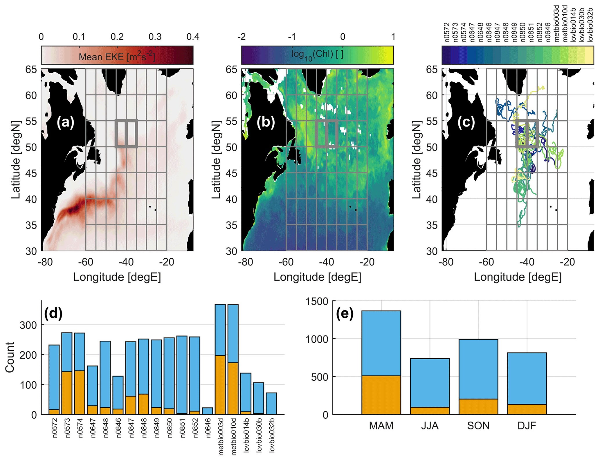
Figure 1Overview of study domain and float sampling showing (a) the temporal mean geostrophic eddy kinetic energy from altimetry, (b) a snapshot of log10(Chl) to convey a typical bloom (June 2002; from GlobColour), (c) the locations of all float tracks, and (d) the counts of all profiles (total height). The orange region counts profiles with a quasi-planktonic index (QPI) < 5 km, and the blue region counts those with a QPI > 5 km. Panel (e) is the same as panel (d), but profiles are binned according to season. In panels (a)–(c), we display the 5∘ × 5∘ space bins used for computing Lagrangian and Eulerian scales. The two bolded space bins in panels (a)–(c) host the rapidly profiling metbio* float segments that are the subject of further analysis.
We include five additional floats that were used to inform NAAMES station sampling but were deployed by other projects (Fig. 1; lovbio* and metbio* floats). Data were obtained as Sprof files from the Argo GDAC, and only profiles overlapping in time with NAAMES were retained. While “Delayed Time” hydrographic profiles were generally available, only “Adjusted” Chl profiles were available, meaning only an automated set of quality checks have been applied (Schmechtig et al., 2018). Samples with QC flags of 1, 2, 3, 5, and 8 are retained, and the profiles are interpolated as with the NAAMES floats. Throughout, special attention is paid to brief (∼ 50 d) segments from metbio003d and metbio010d that exhibited consistently frequent and shallow profiling, as they may exhibit more closely Lagrangian behaviour.
For all floats, the mixed-layer depth (MLD) is computed as the depth at which the potential density exceeds that at 10 m by 0.03 kg m−3. To make float-measured Chl consistent with satellite-measured Chl, we construct a single time series with a weighted average over one attenuation depth, utilizing the fact that about 90 % of the satellite-measured Chl signal in the open ocean comes from a depth of Kd, where Kd490 is the diffuse attenuation coefficient at 490 nm (Gordon and McCluney, 1975). We estimate Kd490 following Morel et al. (2007; their Eq. 8):
where we take [Chl] as the mixed-layer average chlorophyll. We then take a weighted vertical average at each time step as follows:
The series is log-transformed and then smoothed with a running 48 h Hamming window to remove sub-daily variability. Float velocities are estimated by centred differencing profile positions, and the QPI is calculated for each profile as described in Appendix A.
3.2.2 Satellite data
We use the multi-satellite merged altimetry dataset distributed by Copernicus Marine Environmental Monitoring Service which includes daily maps of surface geostrophic velocity and geostrophic velocity anomalies on a 0.25∘ grid (Taburet et al., 2019; Copernicus Marine Environment Monitoring Service, 2021). Geostrophic velocities are used for particle advection when computing the QPI and for comparison to effective float or drifter velocities. The geostrophic velocity anomalies (from sea level anomalies relative to a long-term mean) effectively isolate the mesoscale and are used for computing scales Te and Le. A high pass filter is applied to each anomaly time series by Fourier transforming and zeroing out frequencies lower than (150 d)−1 before inverse Fourier transforming back to the time domain.
We obtain fields of log-transformed, daily, 0.25∘, L3m Chl fields from GlobColour computed from the Garver–Siegel–Maritorena (GSM) algorithm and blending all available satellites (ACRI GlobColour Team, 2020). We use a spatially coarse and blended product to maximize data coverage, with the 0.25∘ resolution consistent with our focus on mesoscale variance. All maps are assumed to correspond to 12:00:00 UTC. The time domain for all satellite data is January 2003–December 2016 and approximately follows the Glover et al. (2018) study.
3.2.3 Drifters
The 6 h surface drifter trajectories within the time domain of the satellite data were obtained from the NOAA Global Drifter Program (Lumpkin and Centurioni, 2019). The dataset reports velocities obtained by centred differencing positions. To remove the influence of inertial oscillations and tides, which can decrease Tl compared with fluctuations due to mesoscale processes, we filter every drifter velocity series with an ideal low pass filter by zeroing out all frequencies lower than (3 IP) in the frequency domain, where IP is the inertial period corresponding to the trajectory's median latitude. For series with gaps, the filter is applied to individual segments as long as they are longer than 20 d. Finally, the filtered time series are subsampled once per day: at 00:00:00 UTC for comparison with the altimetry fields or at 12:00:00 UTC for comparison with the ocean colour fields. We construct Lagrangian time series of Chl by bilinearly interpolating the daily mesoscale Chl maps onto the subsampled drifter returns.
3.3 Subtrahends for chlorophyll
A subtrahend is a field to be subtracted from another. To isolate mesoscale Chl variability, all Chl integral scales are computed from anomalies relative to one of two Chl subtrahends that we construct: a smoothed space–time running filter or a climatology. More details of the methodology and an example time series are given in Appendix B.
The first subtrahend (“smoothed”) is meant to replicate that used by Glover et al. (2018) so that we can obtain Lagrangian and Eulerian timescales consistent with their Eulerian space scales. All GlobColour space–time fields are convolved with a 3-D filter defined as a 31 d Hamming window in time and a 2-D Gaussian in space with a 1∘ full width at half maximum (FWHM) and a 2∘ cutoff. For drifters, the anomalies are projected onto the drifter tracks. For floats, we perform a weighted running average of each float Chl series with weights defined by a 31 d Hamming window. The objective of the space–time filtering in Glover et al. (2018) was to isolate mesoscale (and any resolved submesoscale) variability signals (anomalies) from the lower-frequency seasonal and geographic patterns of bloom formation and decline that were meant to be captured in the subtrahend. However, the short 31 d time window may have the undesirable effect of retaining some of the mesoscale signal in the subtrahend, instead isolating faster processes in Chl anomalies. Yang et al. (2020) found that phytoplankton accumulation rates r are typically 1–2 orders of magnitude smaller than growth rates so that intraseasonal r−1 is generally of order 10 d. Similar physical timescales are found for lifetimes (weeks; Chelton et al., 2011; Gaube et al., 2014) and inverse growth rates (days to weeks; Smith, 2007) of energy-containing mesoscale eddies.
Given those concerns, the second subtrahend is meant to strictly isolate anomalies from a repeating annual cycle (“climatology”). All GlobColour space–time fields are “stacked” by day of year in a fourth dimension (for example, 1 January of every year is regarded as having the same time coordinate) and convolved with a 4-D filter defined as a 31-day-of-year Hamming window in time, a 2-D Gaussian in space with a 1∘ full width at half maximum and a 2∘ cutoff, and a boxcar function (equal weights) across years, yielding a set of 366 maps. For drifters, the anomalies are projected onto the drifter tracks. For floats, the subtrahend is projected onto the float tracks, regressed against float data to account for different data dynamic ranges, and differenced.
3.4 Integral timescales
Our goal is to obtain estimates of the Lagrangian and Eulerian integral timescales of velocity and Chl representative over a 5∘ × 5∘ bin for each measurement platform (Table 1). For all platforms (floats, drifters, and satellite-derived fields), all individual time series of variable y(t) (zonal [u] or meridional [v] velocity or Chl anomalies) are broken into 120 d segments (365 d for Eulerian ocean colour) and each segment is prewhitened, either by removing the scalar mean (Chl anomaly series) or a linear trend line fit by regression (velocity series), creating y′(t) with zero mean. The latitude–longitude coordinates for each time series segment are defined as the median latitude and longitude over the segment length for drifting platforms (float and drifters) or as the pixel latitude and longitude.
Integral timescales are estimated from autocorrelation functions (ACFs). For zero-mean data, the discrete autocovariance function (ACVF) at lag τ is
where N(τ) is the number of data points in separated by . To arrive at an ACF, C(τ) needs to be normalized by the variance, which explicitly is . However, for unevenly spaced (equivalently gapped) data, dividing by can lead to ACF values greater than 1. Because is stationary, and the normalization issue can be avoided by dividing C(τ) by a measure of the variance using only the data points that went into the calculation at lag τ:
where
At this point, we could obtain the integral scale T by integrating R(τ) to the lag of its first zero crossing, which (for a discrete ACF) is . Applying this method to all segments i from all time series in some space subset I (e.g. a 5∘ × 5∘ bin), we could then obtain average scales by averaging estimates from all i∈I. An alternative approach to obtain a spatially averaged scale would be to first construct a single composite ACF that is representative of I and then integrate that single ACF to its first zero crossing. To construct such an ACF, we use pairs of points from all locally prewhitened segments to construct a composite , where
and
For this composite ACF, . For any dataset involving satellite ocean colour, Tc must be used due to the large number of gaps. For evenly spaced datasets, we find , but Tc can be quite different from for the floats with biased larger. This is because weighs each segment i equally, but segments with shorter median Δt between profiles contribute more to Rc(τ) than those with a longer median Δt by virtue of offering more data pairs. In this regard, Rc(τ) is a better estimate of the ensemble ACF, and Tc is a better estimate of the ensemble integral scale. However, there is value in continuing to use when possible, as this reverse order of operations enables us to construct average scales weighted by (QPI)−2, allowing us to gauge in parameter space how a smaller median QPI over the window size affects the turbulence regime experienced by the floats.
All timescales analysed in this study are derived by averaging in space (from integrating Eq. 8 and averaging), except any scales involving satellite ocean colour, where large numbers of gaps require using space-composited ACFs (from integrating Eq. 9). Each method uses all segments in the 5∘ × 5∘ space bins depicted in Fig. 1. Velocity timescales are computed separately for each component (zonal and meridional) before taking (similar for Te). Velocity standard deviations are computed by evaluating the segment standard deviation of each component, averaging them over all segments in a space bin to yield and , and then taking . Finally, Lagrangian length scales are computed by multiplying Lagrangian time and velocity scales together as or .
3.5 Integral length scales
There are 20 × 20 altimetric geostrophic velocity anomalies per 5∘ × 5∘ space bin, per map. For each space bin, we subtract the scalar spatial mean from all points (yielding y′(r)) and compute the distances between all possible pairs of points to construct a radial (isotropic) ACF for space lag d at time t:
where
and
R(d) is integrated in the same manner as R(τ) to obtain an integral length scale L. This is repeated for one map per month over the study period (taken as the 15th of each month), and scales from each map are averaged to obtain and . As with timescales, scales for velocity are defined as the average of zonal and meridional scales, .
For computational reasons, our estimates of Le,Chl in each space bin come directly from the variograms calculated from daily, mesoscale-isolating MODIS fields by Glover et al. (2018). While their analysis used variograms to interpret scale, it is easy to show (Appendix C) that a measure mathematically identical to integrating the ACF to its first zero crossing can be derived from the variogram parameters. To match the length scales defined by Middleton (1985), all Eulerian integral length scales (velocity and Chl) are multiplied by 2.
3.6 Chl frequency spectra
Due to limitations of the data, ACF-derived scales might be biased large (float scales due to large lag bins necessary for uneven sampling; Table 1) or short (ocean colour scales due to poor intra-segment estimates of the mean for sparse segments). Because the power spectrum P(f) is the Fourier transform of the ACF, a time series with an exponential ACF has power spectrum
which depends only on decorrelation time T. This spectrum is characterized by a f0 power law at low frequencies and a f−2 power law at high frequencies, with (2πT)−1 setting the transition frequency. For an independent measure of the power spectrum (that does not rely on our estimated ACFs), spectra will be calculated on all Chl time segments (same segments used for ACFs) using the Lomb–Scargle method (Glover et al., 2011). The frequencies evaluated are the equivalent of the Fourier harmonics for the segment length, and spectral estimates are retained for , which is an effective Nyquist frequency based on the average separation between data points over the segment. For each platform, valid individual spectra are averaged together (ocean colour segments with at least 50 % good samples; float segments with at least 24 profiles).
4.1 Velocity analysis
4.1.1 Quasi-planktonic index (QPI)
The QPI methodology is illustrated in Fig. 2, where we display two examples when a float was located near straining maxima at the intersection of attractive and repulsive flow features. These are regions of rapid tracer stretching, as evidenced by the elongation of synthetic particle clouds, and represent a good challenge for a profiling float to keep up with surface flows. In the case depicted in Fig. 2a where the time spanned by the three adjacent profiles is only 2 d, the QPI is small at 4.49 km. The distribution of the QPI for all float profiles is continuous and skewed long, with a mode centred at about 0–5 km (Fig. 3a). The net velocities experienced by the floats (by centred differencing their positions) are well-correlated to the surface geostrophic velocities projected onto the float track (zonal and meridional correlation coefficients of 0.79 over all floats) but are systematically smaller by a factor of 2.3 (2.4) for u (v). The samples with a QPI < 5 km (a threshold for display purposes, chosen as a compromise between ensuring a small QPI and having a usable amount of data) tend to fall closer to a one-to-one line (“x” symbols in Fig. 3b). The good correlation suggests that the deeper mesoscale flows that the floats feel are equivalent barotropic, and the nature of their deviations from a surface Lagrangian trajectory are primarily in magnitude of displacement, not in direction. For comparison, net drifter velocities have a slope of nearly 1 with respect to surface geostrophic currents (Fig. 3c) but are no better correlated to them (zonal correlation coefficient 0.75; meridional correlation coefficient 0.72). Scatter about the one-to-one line is partly due to ageostrophic effects.

Figure 2Example true (squares) and shadow (circles) float trajectories for (a) a small quasi-planktonic index (QPI) and (b) a large QPI. In both panels, altimetric geostrophic currents are shown as vectors, initial particle locations are black dots, and final forward (backward) particle locations are blue (orange) dots. The QPI and derivative time window are indicated in the lower right-hand corner.
The two examples in Fig. 2 differ markedly in their QPI, with a derivative time window increase from 2 to 4 d corresponding to a QPI that is ∼ 6 times larger and a float trajectory that is qualitatively different from surface trajectories. The profiling interval exhibits strong control on the QPI, with the QPI increasing nonlinearly with the derivative time window (Fig. 4). This relationship represents a combination of greater time for the float to experience more sluggish velocities at parking depth (seen in Fig. 3b), greater time afforded to integrate vertical shear, and the manifestation of two-particle dispersion statistics under quasi-geostrophic turbulence due to mismatch between the float and synthetic particle initial locations.
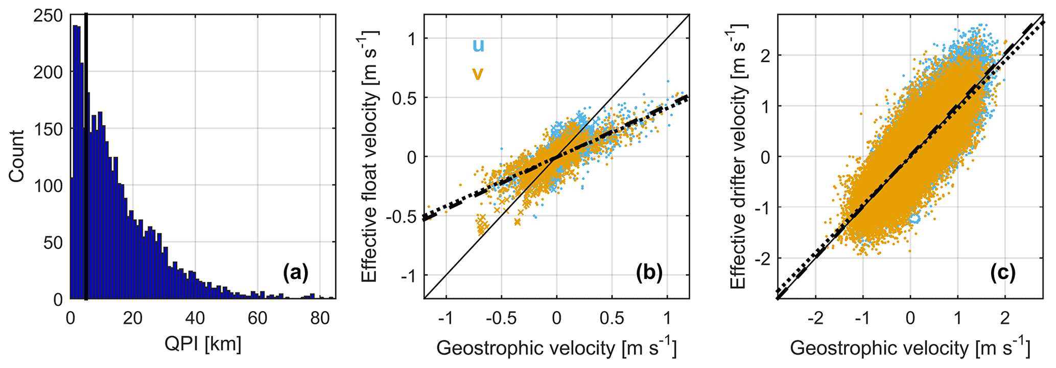
Figure 3Overview of float velocities showing (a) a histogram of the quasi-planktonic index (QPI) for all float profiles (the black line indicates 5 km) and (b) a scatter plot of effective float velocity (centred difference position) against the total surface geostrophic velocity projected onto the float track. Blue (orange) dots are for zonal (meridional) velocity, and similarly coloured x symbols are for profiles with a QPI < 5 km. The solid line is the one-to-one line, and the dashed (dotted) line is the least-squares regression line for zonal (meridional) velocity. Panel (c) is the same as panel (b) but for drifters.
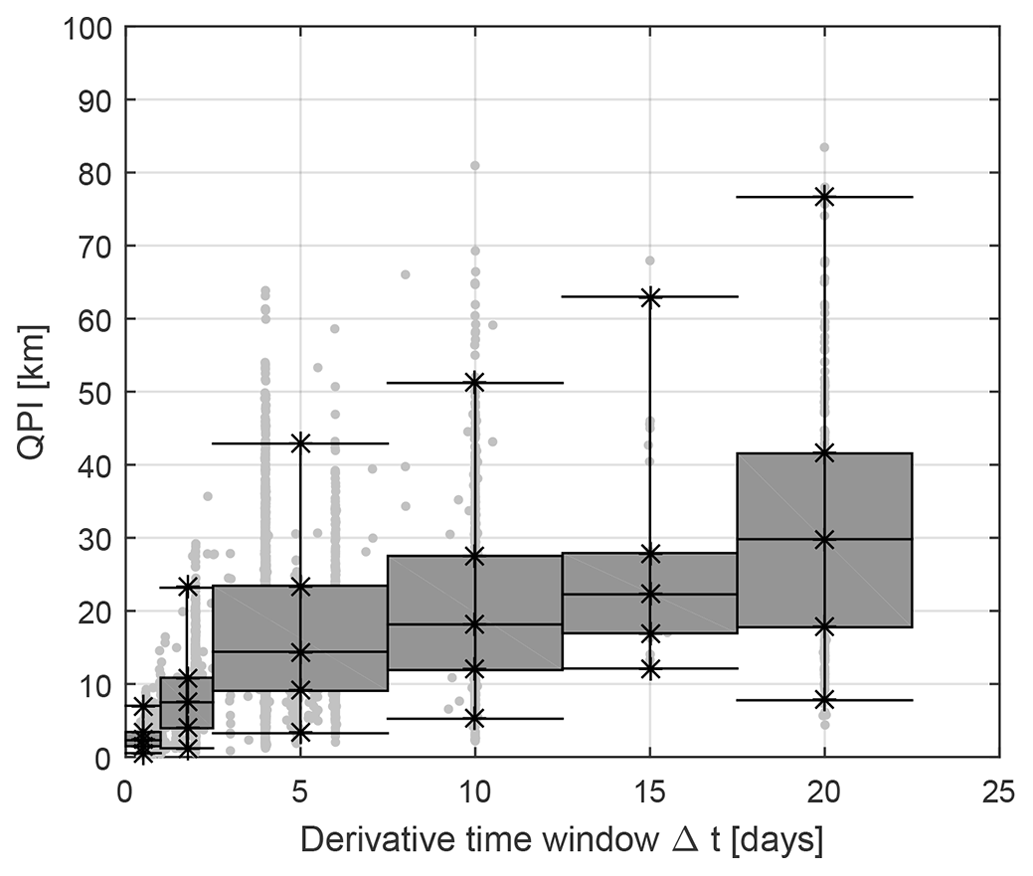
Figure 4Scatter plot of the quasi-planktonic index (QPI) as a function of the derivative time window (time spanned by three profiles) for all float profiles (dots) along with box and whisker plots indicating the 2.5, 25, 50, 75, and 97.5 percentiles. Bins are [0, 1) d, [1, 2.5) d, and then span 5 d after that.
4.1.2 Integral timescales
Evaluating Tl as a function of u′ (Fig. 5a), drifters (open circles) and floats (solid circles) largely cluster into two separate regions, with drifters exhibiting greater velocity variance and a shorter timescale (∼ 3 d compared with the ∼ 5 d of floats). However, for space bins with multiple float segments, when we weight the individual scales by QPI−2 (where the QPI is the segment median; crosses connected by grey lines), we see the cluster of float points moves towards the cluster of drifter points (shorter Tl and larger u′). In particular, the two rapid-time-sampling metbio* float segments (triangles in Fig. 5) reside even closer to the cluster of drifter points than do the QPI−2-weighted values from their host 5∘ × 5∘ bin. Nevertheless, they do not exactly reach the drifter scales of the host bin (open blue and orange circles). Lagrangian integral length scales (Fig. 5c) generally exhibit a similar clustering of points, with floats having shorter length scales and with the QPI−2-weighted points moving towards the cluster of drifter points.
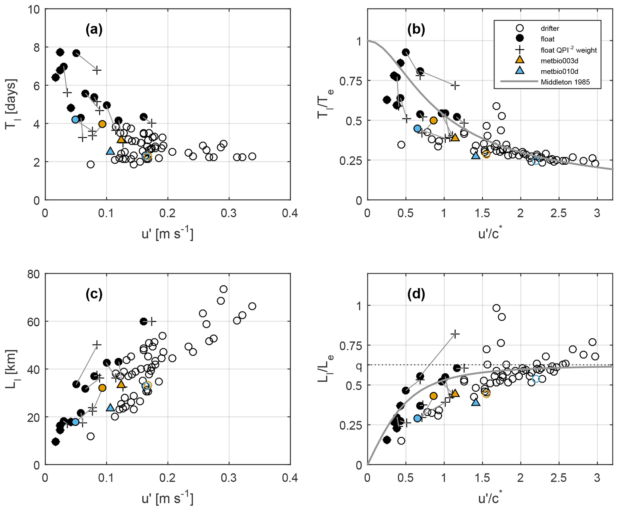
Figure 5Scatter plots of velocity time and length scales for Lagrangian (Tl and Ll) and Eulerian (Te and Le) frames: (a) Tl as a function of scale for the mesoscale eddy velocities, u′; (b) as a function of , where c∗ is the evolution speed for the eddy field, and ; (c) Ll as a function of u′; and (d) as a function of . Hollow (filled) circles come from all surface drifters (all Bio-Argo floats) in a 5∘ × 5∘ bin, and crosses weight the Bio-Argo float-derived scales by QPI−2, with light grey lines connecting the weighted and unweighted values. Coloured triangles come from two time segments from two floats (metbio003d – orange; metbio010d – blue) with frequent and shallow profiling. The float and drifter circles coloured in the same manner are scales corresponding to the 5∘ × 5∘ bins hosting those two segments. The solid line indicates the theoretical relation of Middleton (1985).
A similar relationship is found when examining as a function of (Fig. 5b). There are two clusters of points (floats and drifters) which each reside on the theoretical curve of Middleton (1985), and the QPI−2-weighted float values move along the curve towards the drifter values. The same is generally true for as a function of (Fig. 5d). These results suggest that drifters are generally in the “frozen-field” regime of turbulence, whereas floats are primarily in the “fixed-float” regime, effectively acting as moorings. We found the floats to exhibit a continuum of behaviour, with segments characterized by a smaller median QPI (trajectories more similar to a surface Lagrangian trajectory) residing closer to drifters in and versus space. Overall, this is consistent with the currents experienced by the floats being just as well-correlated to surface geostrophic currents as are the currents experienced by surface drifters (Fig. 3); this suggests that Te calculated from mesoscale geostrophic velocity anomalies derived from altimetry is a good estimate for both the surface and deep flow, and the mesoscale currents are generally equivalent barotropic with only a small horizonal wavenumber attenuation over depth. Floats generally traverse the eddy field more sluggishly than a surface parcel (but in a manner still aligned with the surface flow), and this will impact how they sample a reactive tracer.
4.2 Chlorophyll analysis
4.2.1 Chlorophyll scales relative to the smoothed subtrahend
Relative to the smoothed subtrahend, both floats and drifters experience , even though drifters move faster than floats, so the Chl field is evolving faster than either platform moves (Fig. 6). This suggests that the primary balance in the material derivative should be an approximate correspondence of the Eulerian and Lagrangian tendency terms, EUL ≈ LAG (Eq. 5). We see that this is the case, for example, for drifters with ocean colour in the two space bins that host the rapidly sampling metbio* segments (Fig. 7a, b; see locations as bolded bins in Fig. 1a–c). The eddy advection term (ADV) is about 25 % the magnitude of either EUL or LAG and is presumably less important. Drifters sample EUL ≈ LAG, whereas floats sample LAG < EUL, except for the rapidly profiling metbio* segments during which the float is behaving most like a drifter and EUL ≈ LAG. As the primary balance is EUL ≈ LAG, for drifters is approximately 1 in every space bin (Fig. 6a). The ratio is likely also ∼ 1 for floats, but our ratios are biased large because coarse float time sampling demands using larger lag bins in the ACF (Table 1), causing the structure of the ACF at small lag to be poorly resolved. We know that the float scales are biased large because must approach 1 as (the observer is stationary), but that is not the case. Averaged float scales weighted by QPI−2 are shorter, approaching drifter with ocean colour scales. For both platforms, because EUL ≈ LAG, everywhere (Fig. 6b). That is because neither platform has enough time to traverse Le, Chl before Chl becomes decorrelated. This is corroborated by counting the number of ocean colour pixels traversed by a drifter over Tl, Chl, which is ∼ 1. The composite frequency spectra for both platforms (Fig. 8a, b) reveal good agreement with the model of an exponential ACF with an e-folding time Tl, Chl of between 0.5 and 1 d (dashed reference curves). The similar decorrelation time for both platforms is consistent with the interpretation that EUL ≈ LAG relative to this subtrahend (the different motions of the two platforms do not matter) and is consistent with our interpretation that the float Tl, Chl values computed from the ACFs are likely biased large and, in reality, are closer to the Tl, Chl ∼ 1 d of drifters with ocean colour.
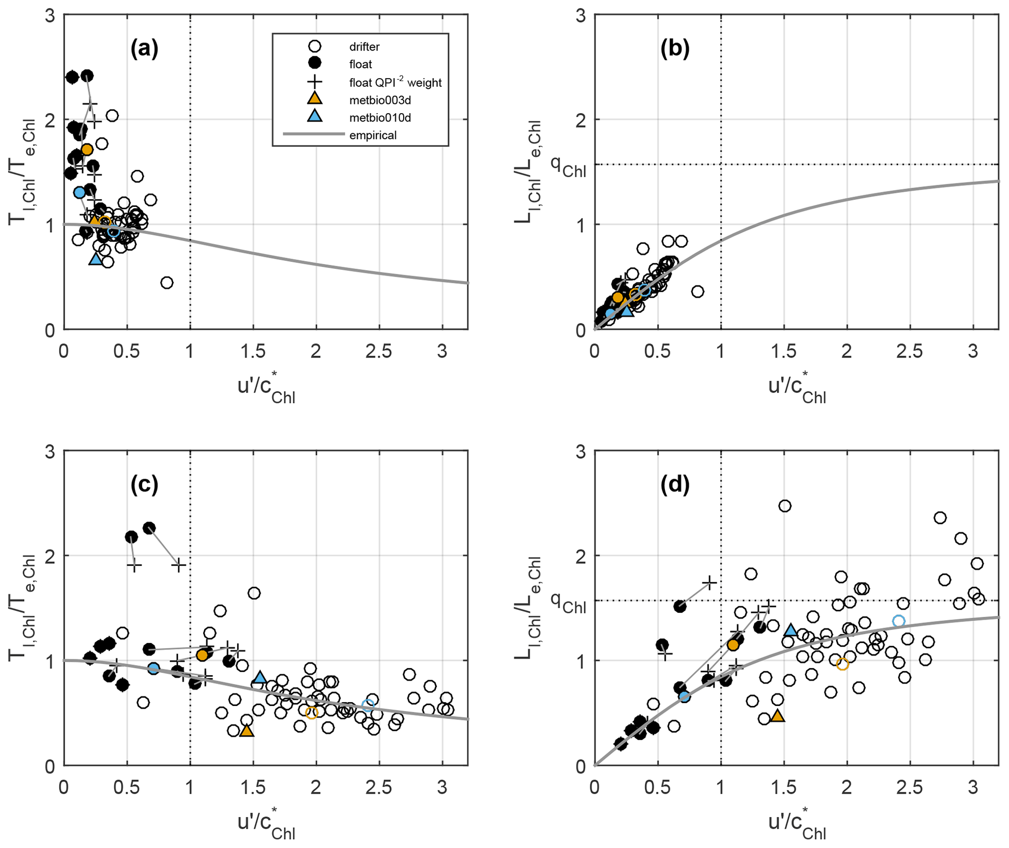
Figure 6Scatter plots of chlorophyll time and length scales for Lagrangian (Tl,Chl and Ll,Chl) and Eulerian (Te,Chl and Le,Chl) frames: (a) as a function of from anomalies relative to the smoothed subtrahend, where u′ is a scale for the mesoscale eddy velocities, and is the evolution speed for the chlorophyll field (); (b) as a function of from anomalies relative to the smoothed subtrahend. Panels (c) and (d) are the same as panels (a) and (b) but for anomalies relative to the climatology subtrahend. Symbols are identified in the legend and are exactly the same as in Fig. 5. Grey curves are from Eq. (12), with and s=2.
4.2.2 Chlorophyll scales relative to the climatological subtrahend
Relative to the climatological subtrahend, floats experience , whereas drifters experience . Therefore, drifters sample Chl space–time fields by traversing mesoscale Chl structures of diameter Le, Chl, whereas floats sample Chl somewhat more like a fixed observer (Fig. 6c, d). Drifters measure , whereas floats measure . Note that this distinction between platforms is similar to what we saw regarding how they each sample the velocity field (compare Fig. 5b and d with Fig. 6c and d), the meaning of which will be discussed in more detail later. With for drifters (and u′ occasionally close to for floats), we expect effects of advection to be important. We see this to be the case, for example, in the two space bins hosting the rapidly profiling metbio* segments (Fig. 7c, d). For drifters with ocean colour, EUL ≈ ADV and each is about 50 %–60 % of LAG in those space bins, confirming that all terms are important. For floats, the ADV term is smaller than it is for drifters (because floats have smaller velocity variance) except for the rapidly profiling metbio* segments which have ADV close in magnitude to drifter ADV. The LAG term for floats tends to be smaller than for drifters, except for the rapidly profiling metbio* segments, for which the term is large like it is for drifters.
As EUL ≈ ADV for drifters, . This is because a portion of the Lagrangian Chl signal is decorrelated by the platform traversing lateral Chl gradients. For floats, because ADV is less important and LAG is reduced, , more closely approximating an Eulerian observer. Consistent with the importance of advection, drifters with ocean colour tend to experience or even greater than 1 in some space bins (Fig. 6d). Drifters can experience because Lagrangian trajectories are often aligned with isolines of tracer (Lehahn et al., 2007); hence, drifters do not move directly down-gradient. Floats, on the other hand, tend to sit on a linear one-to-one line in versus space (Fig. 6d). This is because EUL, not ADV, plays a primary role in the decorrelation because floats move slower than the Chl field evolves, except for the fastest moving floats which plateau where the drifter points do in Fig. 6d. Note that averaged scales weighted by QPI−2 move towards drifter scales in both and versus space (Fig. 6c, d), with increased velocity variance and generally (but not exclusively) shorter Tl, Chl and longer Ll, Chl. Note also that float-based results are not sensitive to ACF methodology (use of Eq. 8 or Eq. 9; Appendix D).
The frequency spectra (Fig. 8c, d) deviate from the theoretical power spectra corresponding to an exponential ACF for any value of Tl, Chl (curves with and 10 d are shown, approximately bracketing the calculated drifter and float scales relative to this subtrahend) and instead take on an approximate f−1 slope over calculated frequencies. Given the role of ADV relative to this subtrahend, one possibility is that the Lagrangian f−1 slope represents a manifestation of an Eulerian wavenumber k−1 slope associated with a passive tracer under quasi-geostrophic turbulence (Smith and Ferrari, 2009) as the platform traverses the approximately frozen field, but this cannot be confirmed. Regardless, an equal spectral slope for both platforms is not inconsistent with our ACF-derived timescales but does mean that we cannot use the spectra to corroborate them.
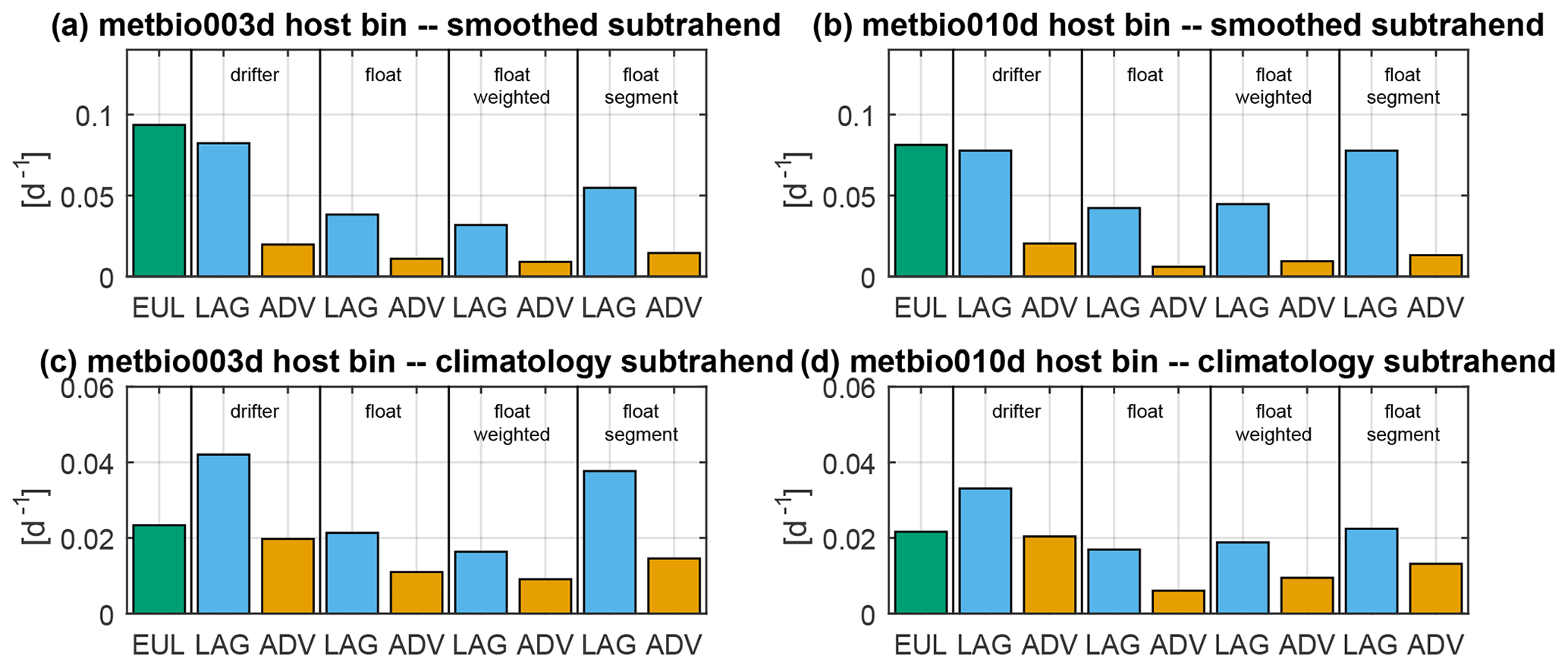
Figure 7Magnitude of the material derivative terms for log-transformed surface chlorophyll using Eq. (5) in the two space bins hosting the rapidly profiling metbio* segments. The Eulerian tendency (EUL, bluish green) term is plotted on the left of each panel, and the Lagrangian tendency (LAG, blue) and eddy advection (ADV, orange) terms are displayed separately for drifters, floats, floats with average scales weighted by QPI−2, and the metbio* segments themselves. Panels (a) and (b) are calculated from Chl anomalies relative to the smoothed subtrahend, and panels (c) and (d) are calculated from Chl anomalies relative to the climatological subtrahend. Panels (a) and (c) are for the bin hosting the metbio003d segment, and panels (b) and (d) are for the bin hosting the metbio010d segment.
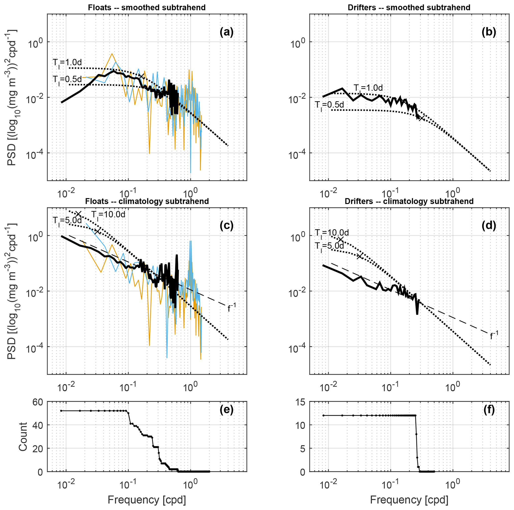
Figure 8Averaged Lomb spectra for chlorophyll from all valid float (a, c, e) and drifter (b, d, f) segments, as defined in Sect. 3.6. Spectra in panels (a) and (b) and panels (c) and (d) are calculated from Chl anomalies relative to the smoothed and climatological subtrahend respectively. Panels (e) and (f) give counts of valid estimates per frequency. For float spectra, the bold black line is the space-averaged spectrum, while the orange (blue) spectrum is from the individual metbio003d (metbio010d) segment. Dotted reference spectra are theoretical spectra for an exponential autocorrelation function (ACF) with a decorrelation time Tl,Chl as labelled. Dashed spectra in panels (c) and (d) give a −1 power law slope.
4.3 Biophysical interpretation of time and length scales
To interpret the meaning of these Chl scales, we compare them to the velocity scales. If stirring by the mesoscale velocity field is a primary driver of Chl variability, we expect the two variables to have similar Eulerian scales. Beginning with the smoothed subtrahend, although the Eulerian space scales of Chl and velocity are similar (Fig. 9b), the Eulerian timescales are unrelated (Fig. 9a; squares), with Te, Chl fixed at ∼ 2 d but Te spanning ∼ 5–12 d. Along a trajectory, Chl decorrelates faster than velocity (Fig. 9c) and over a shorter distance (Fig. 9d) for both platforms, with floats experiencing longer decorrelation times of each variable but covering a shorter distance before becoming decorrelated. Eulerian velocities are calculated from satellite altimetry using a geostrophic balance, therefore containing mesoscale and larger balanced flows, and we note that Lagrangian velocities are from drifter trajectories that were filtered in time to remove fluctuations shorter than 1.5 inertial periods, a procedure that presumably removes primarily unbalanced motions. Hence, all velocity signals are likely dominated by balanced, mesoscale flows. The short time window of the Chl subtrahend (31 d) means that only rapid fluctuations (relative to inverse growth rates of mesoscale baroclinic instability or typical inverse phytoplankton accumulation rates) are retained. While tight coupling between division and loss rates tends to keep accumulation rates r low, abrupt changes in division rates due to rapid changes in environmental conditions can cause large-amplitude fluctuations in r (Behrenfeld and Boss, 2018). Field studies in the subpolar North Atlantic observed near-surface accumulation rates of 0.47 d−1 up to 0.77 d−1 (Graff and Behrenfeld, 2018), corresponding to timescales of 1.3–2.1 d. Dynamically, submesoscale processes have length scales on the order of the deformation radius of the mixed layer (of order 1 km) and timescales on the order of an inverse inertial period (of order 1 d) (Mahadevan, 2016), scales smaller than an ocean colour pixel and shorter than those of mesoscale dynamics. Hence, the EUL ≈ LAG balance for Chl relative to this subtrahend can be taken as dominance of ocean colour pixel-scale variability in the retained signal due to either submesoscale processes or biological sources/sinks.
For the climatological subtrahend, the Eulerian length scales are the same as relative to the other subtrahend; thus, again, . However, for this subtrahend, (Fig. 9a; circles). This is consistent with mesoscale dynamics setting the Eulerian statistics of both velocity and Chl. Along a trajectory, Chl decorrelates more slowly than velocity, and Chl is correlated over a longer distance than velocity. The Lagrangian timescale for floats is greater than it is for drifters, as the reduced importance of the ADV term means that Chl properties are retained longer. The equivalence of Eulerian time and length scales of velocity and Chl suggests that Chl scales are also dominated by balanced mesoscale dynamics, via advection, and a physical interpretation relating mesoscale stirring to Lagrangian Chl scales will be presented in Sect. 4.5. Because lateral motion and the ADV term are important, the differing motions of floats and drifters means that they each sample different Chl signals relative to this subtrahend, with floats behaving somewhere between an Eulerian and a surface Lagrangian observer. The exception is the two metbio* segments which sample Chl fields much like a surface Lagrangian observer would.
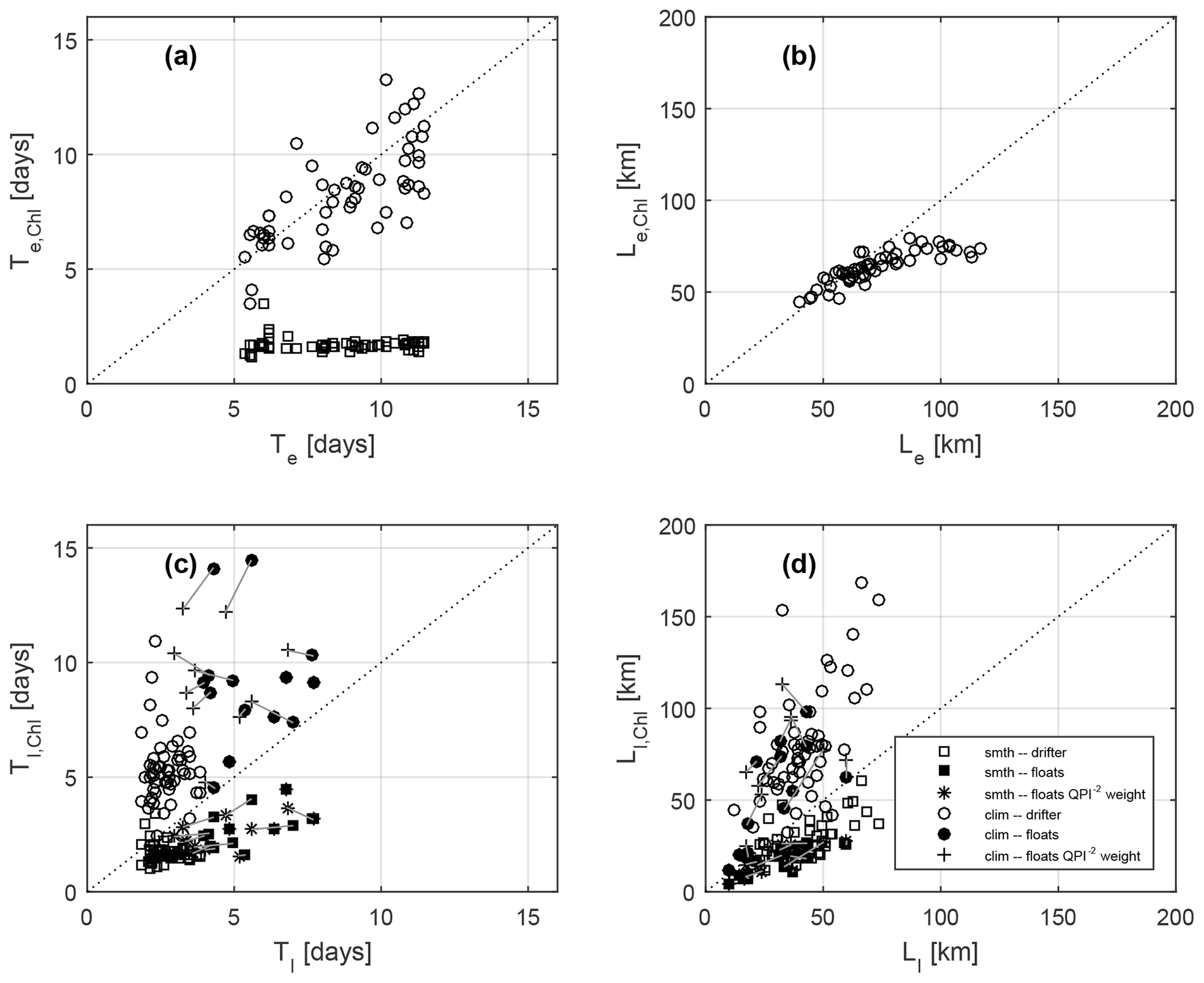
Figure 9Time and length scales of chlorophyll (Chl) and velocity: (a) Eulerian timescales (Te,Chl versus Te); (b) Eulerian length scales (Le,Chl versus Le); (c) Lagrangian timescales (Tl,Chl versus Tl); and (d) Lagrangian length scales (Ll,Chl versus Ll). Open circles are for drifters, filled circles are for floats, and crosses are for floats weighted by QPI−2 where all scales are calculated from Chl anomalies relative to the climatology subtrahend. Open squares are for drifters, filled squares are for floats, and stars are for floats weighted by QPI−2 where all scales are calculated from Chl anomalies relative to the smoothed subtrahend. Dotted lines are the one-to-one lines.
4.4 Comparison with earlier estimates and a role for biology
Few studies have investigated Eulerian timescales of phytoplankton, and even fewer works have addressed Lagrangian timescales. Further, comparison of results across studies is complicated by myriad choices of data processing (e.g. subtrahends), intrinsic data resolution, and methodology (ACF or otherwise). In a series of studies, Denman and Abbott (1988, 1994) analysed a scale-dependent decorrelation time by assessing the spatial coherence of ocean colour images separated in time and found that Eulerian decorrelation times are generally less than about a week, being longer for 50–100 km wavelengths and shorter for 25–50 km wavelengths. Wavelengths smaller than 25 km are decorrelated after about 1 d. Comparing the cross-coherence of Chl and sea surface temperature (SST), they concluded that physical stirring is the major driver of Chl variability at the mesoscale, a conclusion shared by Glover et al. (2018). In a more recent study, Kuhn et al. (2019) assessed Eulerian temporal decorrelation of numerically modelled biomass and found decorrelation times to generally be about 15 d (longer in regions of lower eddy kinetic energy and for larger phytoplankton size classes). Their longer decorrelation times may be partially due to analysing 3 d averaged model fields. Our Te, Chl values fall into this broad range. The stark difference in values relative to the two subtrahends may be partially explained by the wavelength-based analyses of Denman and Abbott (1988), whereby the smoothed subtrahend is emphasizing pixel-scale (∼ 25 km) variability, contributing to the short (∼ 1–2 d) Te, Chl compared with the climatology subtrahend (∼ 5–12 d).
Estimates of Tl, Chl are rarer. Abbott and Letelier (1998) used bio-optical surface drifters in the California Current and found that Tl, Chl and Tl in the open ocean are both about 2.5 d whereas Tl, SST is closer to 7 d, causing them to question the degree to which Chl behaves as a passive tracer. Boss et al. (2008) found much longer Tl, Chl of about 2 weeks using a profiling float. We also find Tl∼ 2–3 d for drifters (longer for floats), but Tl, Chl is systematically larger or smaller depending on the subtrahend (note that Abbott and Letelier, 1998, detrended float segments, whereas Boss et al., 2008, only removed a scalar mean, with the latter observing that seasonality dominated their longer decorrelation time). In a series of studies, Jönsson et al. (2009, 2011) used synthetic particle trajectories and satellite ocean colour to quantify terms of the material derivative. They found that the advective term is generally comparable in magnitude to the Lagrangian tendency and must be included. There are important differences in the magnitude and sign of each term, where a near-zero Eulerian tendency can be explained by a large Lagrangian tendency countering an advective term.
Analyses of Lagrangian series point to an importance of biological sources and sinks. Advection of phytoplankton across spatial gradients of environmental conditions will affect dominant phenotypes (Lévy et al., 2014), with the relative timescales of physical parameters and physiological acclimation governing species succession (Zaiss et al., 2021). The LAG term is generally the largest term in the scaling of Eq. (5) (Fig. 7), meaning that turbulent diffusion or sources and sinks of Chl are important. Relative to the smoothed subtrahend, as discussed earlier, the appropriate spatial scales are not resolved, and an approximate balance of LAG ≈ EUL is achieved. However, relative to the climatological subtrahend, the magnitudes of LAG and ADV tend to scale with each other, being largest for drifters and the metbio* segments and smallest for the unweighted float segments (Fig. 7). By moving slower than phytoplankton patches, floats underestimate sources and turbulent diffusion (reducing LAG); thus, there is less Chl variance apparently advected (reducing ADV, where we interpret platform speed as the typical speed of velocity fluctuations). Note that this is consistent with the interpretation posed in Sect. 4.3: effects of turbulent diffusion and sources and sinks are contained in the information content of ocean colour space–time fields and will project onto an Eulerian tendency or an advective term depending on the relative rates at which a phytoplankton patch and observer move. It remains to be seen which of turbulent diffusion (DIFF) or sources (S) is important in driving the decorrelation, and this will be addressed in Sect. 4.5.
Finally, comparing Lagrangian and Eulerian timescales of Chl and of phytoplankton biomass (from backscattering) reveals regional discrepancies, confirming that Chl contains an acclimation component; however, each variable has a similar ratio of Lagrangian-to-Eulerian timescales, confirming that they are sampled by a moving observer in the same manner and giving us confidence in our Chl-based biophysical interpretation (Appendix E).
4.5 Empirical relationship between chlorophyll Lagrangian and Eulerian scales
The plots of and as functions of (Fig. 5b, d) and and as functions of (Fig. 6c, d) have the same general shape. A similar functional dependence is not surprising given correspondence of Eulerian time and length scales for both velocity and Chl (Fig. 9a, b), with only subtle differences in the Lagrangian time and length scales of each variable (Fig. 9c, d) accounting for differences in the underlying functions. For this reason, we posit that a mesoscale relationship for Chl may take the same form as that Middleton (1985) derived for velocity:
Here, the constant qChl sets the asymptotic value at large αChl, and the exponent s sets how rapidly G transitions between linear and constant behaviour. In the velocity scaling (Eq. 3) of Middleton (1985), the asymptotic value q is less than 1 because the variable being decorrelated is the same variable causing the decorrelation and Ll never reaches Le. For Chl, one possibility is to set qChl=1 so that as ADV dominates we have . However, we have seen that Ll,Chl is routinely greater than Le,Chl. A better choice (purely empirically) seems to be so that as ADV dominates we have (grey curves in Fig. 6). For simplicity, we set s=2.
The observation shows that the Chl field is characterized by features with scales similar to mesoscale eddies. To take this a step further, Glover et al. (2018) showed that, in our study region of the North Atlantic, the statistical decorrelation length Le,Chl is proportional to a mixing length that quantifies the distance that a mesoscale eddy could stir a water parcel containing Chl anomalies, assuming that all Chl anomalies are generated by stirring a mean gradient (see their Fig. 7). This provides a further clue that mesoscale stirring might be of primary importance in setting Lagrangian Chl statistics. The effects of stirring should be most apparent in the asymptotic limit as turbulent velocity fluctuations are larger than the evolution speed of the Chl field. Because Chl isolines twist and deform as they are strained by the mesoscale field, can exceed Le,Chl. To motivate an empirical value relating the frames, we appeal to an idealized geometry of mesoscale eddies. Following the convention of Middleton (1985), Le equals twice the decorrelation length and is effectively a mesoscale eddy diameter. From this perspective, serves as a radius of curvature for the maximal (half a circumference) of a parcel traversing the perimeter of a mesoscale eddy as it is stirred. Half a circumference may be a meaningful decorrelation length in the scenario where a mean Chl gradient is stirred by an eddy of diameter Le, partitioning the eddy into two hemispheres of high and low Chl respectively (e.g. see Fig. 2a of Gaube et al., 2014) and effectively equating the Eulerian separation Le,Chl in Euclidean space to a trajectory distance Ll,Chl. At the other asymptotic limit, if , turbulent velocity fluctuations relative to the translation of the Chl field are small and so that . With this interpretation, it is useful to view ADV as a local stirring of a mean Chl field instead of advection of anomalies over long distances (although the equivalence of Le,Chl and a mixing length shown by Glover et al., 2018, relates the two perspectives). This is why the effect of u′ on matters in its relation to , which is an evolution speed for the scalar field. Likewise, it is useful to view u′ as turbulent velocity fluctuations, which by our filtering are associated with the mesoscale eddy field. When the observer is a true surface Lagrangian observer, u′ is properly captured by the platform's motion; however, as we have shown, for an Argo float, the effects of stirring are underestimated.
The relationships in Eq. (12) reveal further insight into the processes that cause the Lagrangian decorrelation of Chl. The turbulent diffusion term from Eq. (1) (DIFF) can be expressed as a Fickian diffusion with coefficient K that is constant over an integral timescale:
In the Lagrangian frame, the diffusivity K scales as (Taylor, 1922), allowing us to scale DIFF as follows:
If we define a parameter β as the ratio of the total Lagrangian tendency to the contribution from turbulent diffusion, we obtain the following scaling:
This says that β is equal to the square of the ratio of the Eulerian length scale of Chl to the geometric mean of the Lagrangian length scales of Chl and of velocity. From our Fig. 9d, relative to the climatology subtrahend, we have so that we can rewrite β as follows:
If we consider the case where LAG is entirely driven by DIFF (β=1), we have
It is worth noting that the asymptotic value (for , heuristically argued for above, is , which is quite close to 2.5. This suggests that, in the limit of large turbulent velocity fluctuations (where , we have Ll,Chl (and hence Tl,Chl) determined entirely by turbulent diffusion. Because is globally less than or equal to qChl (Fig. 6d; Eq. 12), we can obtain an inequality for β, revealing that β= LAG DIFF is globally greater than or equal to 1, or equivalently LAG ≥ DIFF. This must be true because, from Eq. (1), LAG = DIFF +S. As an extension of this result, it is implied that S becomes increasingly important in setting Lagrangian decorrelation where (as β≫1), and this happens in the limit that turbulent velocity fluctuations are relatively small (). Therefore, in short, we have confirmed our earlier interpretation that when , DIFF drives Lagrangian decorrelation Tl,Chl as a consequence of mesoscale stirring, and when , sources S (biological or otherwise) drive Lagrangian decorrelation.
4.6 Methodological decisions
Many methodological decisions were made in this study. Here, we discuss some of them and comment on how they may influence our results.
4.6.1 Depth reduction of float time series
As described in Sect. 3.2, the Chl time series constructed from the float measurements are weighted by depth to better approximate what satellites see, allowing us to compare scales derived from floats to those derived from ocean colour. We found that using float series calculated as a more traditional (and biophysically meaningful) depth average over the mixed layer (e.g. Yang et al., 2020) yields results that are not appreciably different from those in Figs. 6–9.
4.6.2 ACF parameters
Although the methodology is consistent, the segment length and ACF bin sizes vary for different platforms (Table 1). Lagrangian segments should be kept as short as possible because a platform may encounter different environmental (physical or otherwise) conditions as it moves; we followed Lumpkin et al. (2002) and used 120 d for all variables. For Eulerian series, this is less of an issue, and, as seasonal variability is removed, the length of the segment is less likely to have a significant impact on scales. Hence, we used 365–366 d segments for Chl. Regarding temporal ACF bin sizes, ideally one would use a bin size that matches the sampling interval because this is the smallest lag that can be resolved. For this reason, the ACFs based on satellite altimetry, satellite ocean colour, or drifters use a bin size of 1 d. The floats have a variable profiling interval (Fig. 4). While they sometimes profile with a frequency of about once per day, they generally profile less frequently, and we settled on a bin size of 5 d. The two metbio* float segments are given special attention because they profiled more frequently; for that reason, we were able to use a finer bin size of 1 d. As a general statement, choosing a larger bin size causes the structure (curvature) of the ACF to be poorly resolved at short lag and biases timescales large, as discussed in Sect. 4.2. A similar rationale applies to the spatial ACF bin size, where 27.8 km approximately corresponds to the 0.25∘ resolution of the data in the latitudinal direction. The scales are averaged in (or the ACFs are composited in) 5∘ × 5∘ space bins to enhance the quality of estimates, and this size was chosen to match the grid size of Glover et al. (2018), who computed variograms of Chl and found this size good to resolve spatial variability.
4.6.3 Ocean colour product
There is a trade-off between resolving more variance and dealing with increased gaps when moving to a finer-resolution ocean colour product. For the purpose of this study, we chose to prioritize data coverage, leading us to select a blended, 0.25∘ product, and focus on the mesoscales. The choice of product is also consistent with the grid size of the Eulerian velocity field (0.25∘ altimetric geostrophic currents), which is important because we compare the two variables (Fig. 9). In particular, GlobColour was selected because Zhang et al. (2019) demonstrated it to resolve realistic Lagrangian behaviour in terms of (sub)mesoscale dynamics, so we conclude that its space–time information is biophysically accurate.
We suspect that our findings depend on our choice of ocean colour product and constitute a representation of mesoscale biophysical dynamics: studies using submesoscale-resolving velocity and ocean colour data may find different relationships between Lagrangian and Eulerian scales. In particular, we suspect that the finding is indicative of mesoscale variance and a consequence, in part, of an 0.25∘ ocean colour product. This may be the manifestation of an observer moving across gradients in the mean chlorophyll field, as would happen when a mesoscale eddy stirs a horizontal gradient as discussed in Sect. 4.5, and is consistent with the importance of DIFF – a manifestation of unresolved advection – in driving the Lagrangian decorrelation over most of the range of observations instead of S. Chlorophyll may actually be conserved for longer along a trajectory than our results would indicate: if patches are organized in filaments not fully resolved in a 0.25∘ product, the inability of a drifter-projected time series to resolve near-constant chlorophyll levels along a filament will result in an early temporal decorrelation. The result that the ratio is approximately 1 relative to the smoothed subtrahend (where sub-pixel variability probably dominates) while the ratio is less than 1 relative to the climatology subtrahend supports this interpretation.
We analysed the Lagrangian and Eulerian statistics (time and length scales) of velocity and chlorophyll (Chl) as measured by Bio-Argo floats and as represented by satellite ocean colour (GlobColour) projected onto surface drifter tracks. Lagrangian statistics of velocity satisfy the Middleton (1985) relations, with drifters in a frozen field regime (spatial Eulerian decorrelation drives temporal Lagrangian decorrelation) and floats in a fixed-float regime (Eulerian tendency drives decorrelation). However, there is a continuum of behaviour with segments weighted by the inverse square of the quasi-planktonic index (QPI) – a metric quantifying the similarity of a float trajectory to a surface geostrophic trajectory – approaching the frozen-field limit. This is made possible by the mesoscale flows being approximately equivalent barotropic with small horizontal wavenumber attenuation over depth. Given the space–time resolution of our ocean colour product (and typical float time sampling), both floats and drifters sample anomalies relative to the smoothed subtrahend as fixed observers, suggesting that Lagrangian Chl variability is dominated by ocean colour pixel-scale processes at periods shorter than 31 d. Analysis of a finer ocean colour product and a faster sampling observer is necessary to elucidate biophysical mechanisms (e.g. submesoscale sources and sinks). However, relative to a climatological subtrahend, Eulerian decorrelation time and length scales of Chl match those of velocity, suggesting that mesoscale physical dynamics are important in setting plankton distributions, as suggested by earlier studies (Denman and Abbott, 1994; Glover et al., 2018). The ratio of Lagrangian to Eulerian length scales for chlorophyll, , depends on how fast a parcel moves relative to how fast the Chl field evolves , following an empirical curve that appears to have the same functional form as that for velocity but with the asymptotic value replaced by scalar qChl≥1, a value consistent with stirring by mesoscale eddies. A fundamental result of this study is that mesoscale Lagrangian time and length scales are strongly set by the stirring of mesoscale eddies, with turbulent diffusion generally dominating the decorrelation. As for the biophysical interpretation of float-measured time series, qualitatively speaking, the slower horizontal motion of floats relative to surface Chl patch speed means that advection across mean Chl gradients is reduced and both turbulent diffusion and intra-patch biological sources are underestimated, both leading to longer timescales (Tl, Chl) and smaller Lagrangian tendency (LAG) and eddy advection (ADV) terms compared with a surface Lagrangian observer. By choice of data products and filtering, our results are based on time and length scales representative of mesoscale variances in velocity and Chl fields. Follow up studies using data resolving submesoscale variance are warranted.
The quasi-planktonic index (QPI) is a single number that quantifies the similarity of a float trajectory to the best-fit synthetic trajectory (computed by the advection of synthetic particles with altimetric total geostrophic currents) over the temporal footprint of a centred difference derivative (three total float profiles). The procedure is repeated for each float profile i. We first create a disc of particles about by making a rectangle about ri with particles spaced zonally by out to and meridionally by δ0 out to lati±δtotal and then retaining those values with a spherical distance of less than or equal to 0.3∘. We chose and . The disc of K particles is advected by the altimetric total geostrophic currents forward in time with a fourth-order Runge–Kutta scheme at an hourly time step from their initial position at ti to the first hour past float time ti+1. Velocity fields at intermediate time steps are obtained through linear interpolation, and particle velocities are updated through bilinear interpolation in space. For the kth trajectory beginning at float time ti, its position at float time ti+1 is obtained by linearly interpolating its positions at the two surrounding hourly time steps. Similarly, the disc of K particles is advected backward in time with the same fourth-order Runge–Kutta scheme and hourly time step out to the first hour prior to ti−1. For the kth trajectory beginning at float time ti, its position at float time ti−1 is obtained by linearly interpolating its positions at the two surrounding hourly time steps.
The advection gives K sets of three positions at each float step i. The penalty function for trajectory k at float step i measures the average distance between the kth synthetic trajectory and the true float trajectory over the three time steps that constitute the centred difference:
where r is the position in latitude–longitude coordinates, and dist(⋅) is a measure of distance on the sphere. The QPI for time step i is
and has units of kilometres. The corresponding shadow trajectory is the three-element trajectory rk for the k that minimizes S.
Synthetic particle trajectories are advected by altimetric geostrophic currents, which generally approximate the mesoscale flows of interest well. Della Penna et al. (2015) found that including an Ekman term in the advecting flow modified only the tail of the distribution of a QPI calculated against surface drifter trajectories. To gauge how altimetric geostrophic trajectories approximate surface Lagrangian trajectories, we also computed a QPI for all drifter returns in our study space–time domain calculated over Δt=2 d and found that they are larger than expected (median ∼ 8 km). However, the latitudinal variations in the drifter QPI are much smaller than latitudinal variations in the float QPI (the subset with a comparable Δt ∼ 2 d), even though a geostrophic approximation should perform better at mid-latitudes because Ekman transports become more important away from the generally balanced, persistent Gulf Stream and North Atlantic Current and their energetic eddies. This suggests that the median drifter QPI is large not because of failing to include an Ekman term but because geostrophic currents from mapped altimetry data do not resolve inter-swath deformations to the mesoscale field (Ascani et al., 2013) and underestimate surface flows when finite differencing (Sudre and Morrow, 2008). We conclude that the QPI is a useful measure of similarity to surface flow for floats.
The first subtrahend (“smoothed”) is meant to replicate that used by Glover et al. (2018) so that we can obtain Lagrangian and Eulerian timescales consistent with their Eulerian space scales. For Eulerian data, we perform a 3-D convolution of all GlobColour space–time fields with a 3-D filter defined as a 31 d Hamming window in time and a 2-D Gaussian in space with a 1∘ full width at half maximum and a 2∘ cutoff. Just as the total GlobColour data are bilinearly interpolated onto drifter tracks, the subtrahend is interpolated in the same manner, and the two are differenced to obtain Lagrangian Chl anomalies. Finally, for a float Chl subtrahend, we perform a weighted running average of each float Chl series with weights defined by a 31 d Hamming window. This approach to smoothing the float data is less than desirable because it constitutes a Lagrangian subtrahend, whereas the drifter anomalies are about an Eulerian subtrahend projected onto a Lagrangian trajectory. Further, this approach cannot implement an equivalent spatial smoothing in the subtrahend for the float data because they come from a single Lagrangian trajectory (see discussion below). The time filter component of the smoothed subtrahend is effectively a low-pass filter, and, with a cutoff of 31 d, we found it to retain a sizable portion of the intraseasonal (and perhaps mesoscale) variance. This is particularly the case for the float data, where uneven spacing means that the effective cutoff frequency will vary depending on the sparsity of sampling in a 31 d window because data points near the centre of the window are weighted more.
As an alternative, the second subtrahend strictly isolates climatological variability (“climatology”). The spatial footprint of the filter is the same, but the time filtering is performed about a day-of-year coordinate rather than an absolute date coordinate (for example, 1 January of every year is regarded as having the same time coordinate). Specifically, for Eulerian data, we perform a 4-D convolution of all GlobColour space–time fields with a 4-D filter defined as a 31-day-of-year Hamming window in time, a 2-D Gaussian in space with a 1∘ full width at half maximum and a 2∘ cutoff, and a boxcar function (equal weights) across years. Again, the subtrahend is bilinearly interpolated onto the drifter tracks.
The major difference for the climatological subtrahend concerns how the floats are treated. There are not enough co-located floats to create a climatological subtrahend from float-measured Chl, so we construct a float subtrahend from the filtered GlobColour data (Eulerian subtrahend). Because floats measure Chl year-round, whereas GlobColour contains significant seasonal gaps, we first regress annual and semiannual cosines to the Eulerian subtrahend in each pixel as an interpolant. While the inclusion of higher harmonics would yield a better fit in some regions (especially in regions with complex seasonal cycles such as those with spring and autumn phytoplankton blooms), we stick to only the first two harmonics because gaps in the Eulerian subtrahend of up to 6 months would lead to significant overshoot if higher harmonics were included. The resulting field is then projected onto the float tracks (with a simple nearest-neighbour approach in space and time). Finally, because the dynamic range of GlobColour Chl is different from that of the depth-averaged float Chl series, the projected subtrahend needs to be scaled before it can be removed from the float data (like a bias correction). Thus, as a final step, we regress the projected subtrahend against actual float Chl (all samples across all floats) to obtain a best estimate of seasonal cycle amplitude:
A summary of the subtrahends is provided in Table B1, and a visual example of time series is shown in Fig. B1. Anomalies about the climatology subtrahend contain substantially more low-frequency variance, including intraseasonal variability and interannual variability due to year-to-year variations in phasing and amplitude of blooming. The climatology subtrahend has the added benefit of being applied to the floats and drifters in an equivalent manner as an Eulerian subtrahend projected onto a Lagrangian trajectory. It is fair to question whether the smoothed subtrahend as computed for floats is comparable to the smoothed subtrahend as computed for ocean colour pixels and drifters because the former does not include explicit spatial smoothing, only a combined space–time Lagrangian smoothing. As a test, Fig. B1 additionally includes the Eulerian smoothed subtrahend projected onto float tracks (via the nearest-neighbour interpolant and regressed against float data to correct for dynamic range) for periods when we have overlapping data. In general, the projected Eulerian smoothed subtrahend closely agrees with the float smoothed subtrahend. Exact correspondence between float and satellite Chl is not expected because floats sample a parcel of water on the order of the size of the platform, whereas gridded ocean colour products integrate information in space and time (see discussion in Yang et al., 2020).
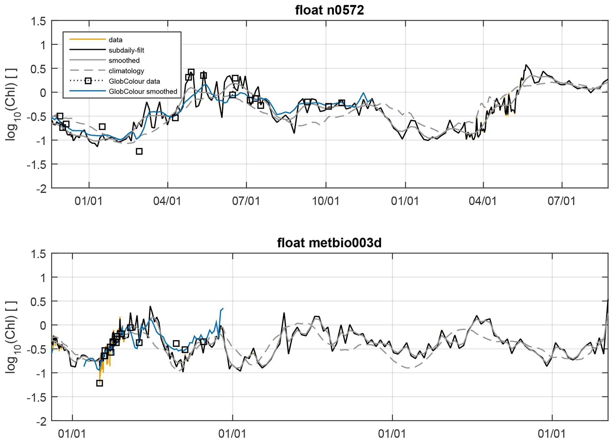
Figure B1Example time series of log-transformed, depth-reduced Chl from two floats (n0572 and metbio003d). Data are orange, data with sub-daily filter applied are black, the “smoothed” subtrahend is solid grey, and the “climatology” subtrahend is dashed grey. For evaluation, we also display the GlobColour data projected onto the float tracks (black squares) and the Eulerian smoothed subtrahend from GlobColour projected onto the float tracks (solid blue). Note that the sample interval was generally over 1 d except for brief intervals so that sub-daily filtered and unfiltered series are generally identical (black curve generally over orange). Note also the variable sample rate for metbio003d, illustrating how the effective cutoff period of the smoothed subtrahend can vary substantially from 31 d.
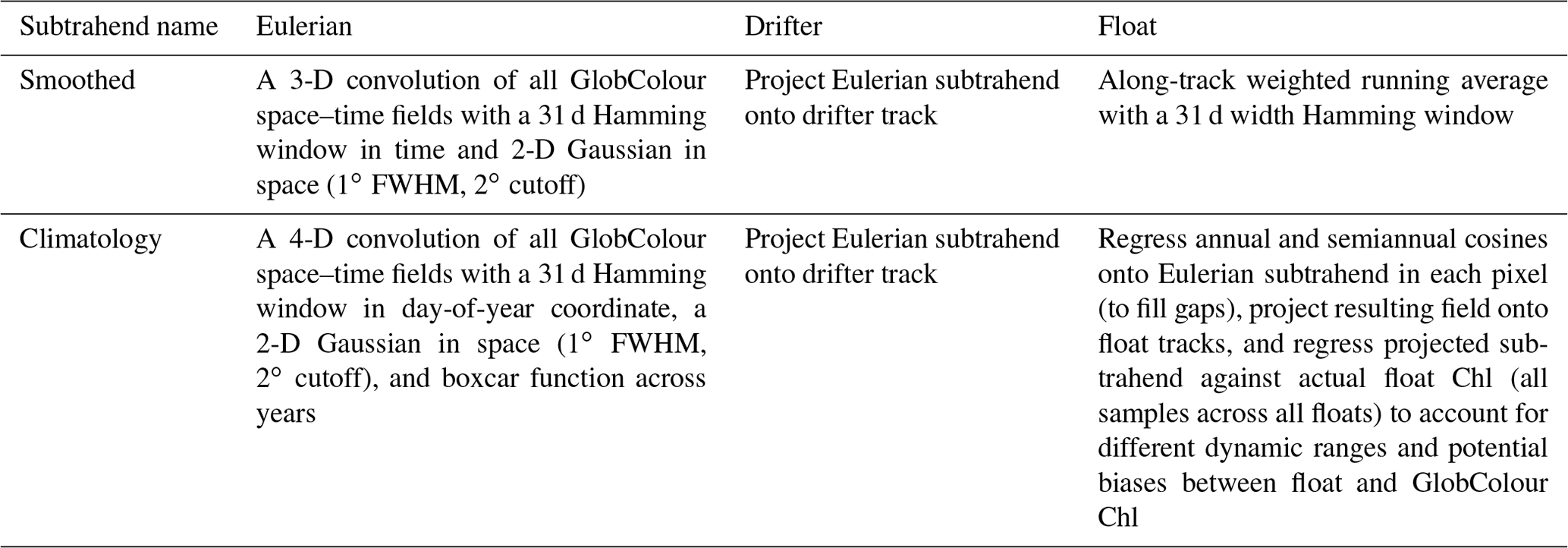
Glover et al. (2018) calculate space scales of mesoscale Chl variability by calculating variograms of mesoscale Chl anomaly fields in 5∘ × 5∘ space bins. They fit a spherical variogram model to their calculations by nonlinear regression, which in 1-D is given by
where c0 is the nugget (unresolved variance), c∞ is the sill (approximating the total variance), a is the range (closely related to the decorrelation length), and δ is the scale of space separation being evaluated (Glover et al., 2011, 2018). Intuitively, a is closely related to the integral decorrelation length (integral of spatial ACF to first zero crossing), but the two are not equal. The spatial autocorrelation function R(δ) is related to the variogram by
where C(δ) is the autocovariance function. Using the fact that C(0)=c∞, the space lag δ0 at which the ACF R=0 is determined by rearranging Eq. (C2) to yield c∞=γ(δ0), requiring δ0=a. Thus, the integral of the ACF to the first zero crossing is given by
which, after substituting in Eq. (C1), gives
Glover et al. (2018) report separate ranges ax and ay from MODIS data in the zonal and meridional directions respectively. Therefore, we calculate zonal and meridional integral length scales Lx and Ly from Eq. (C4) to define the Chl integral length scale,
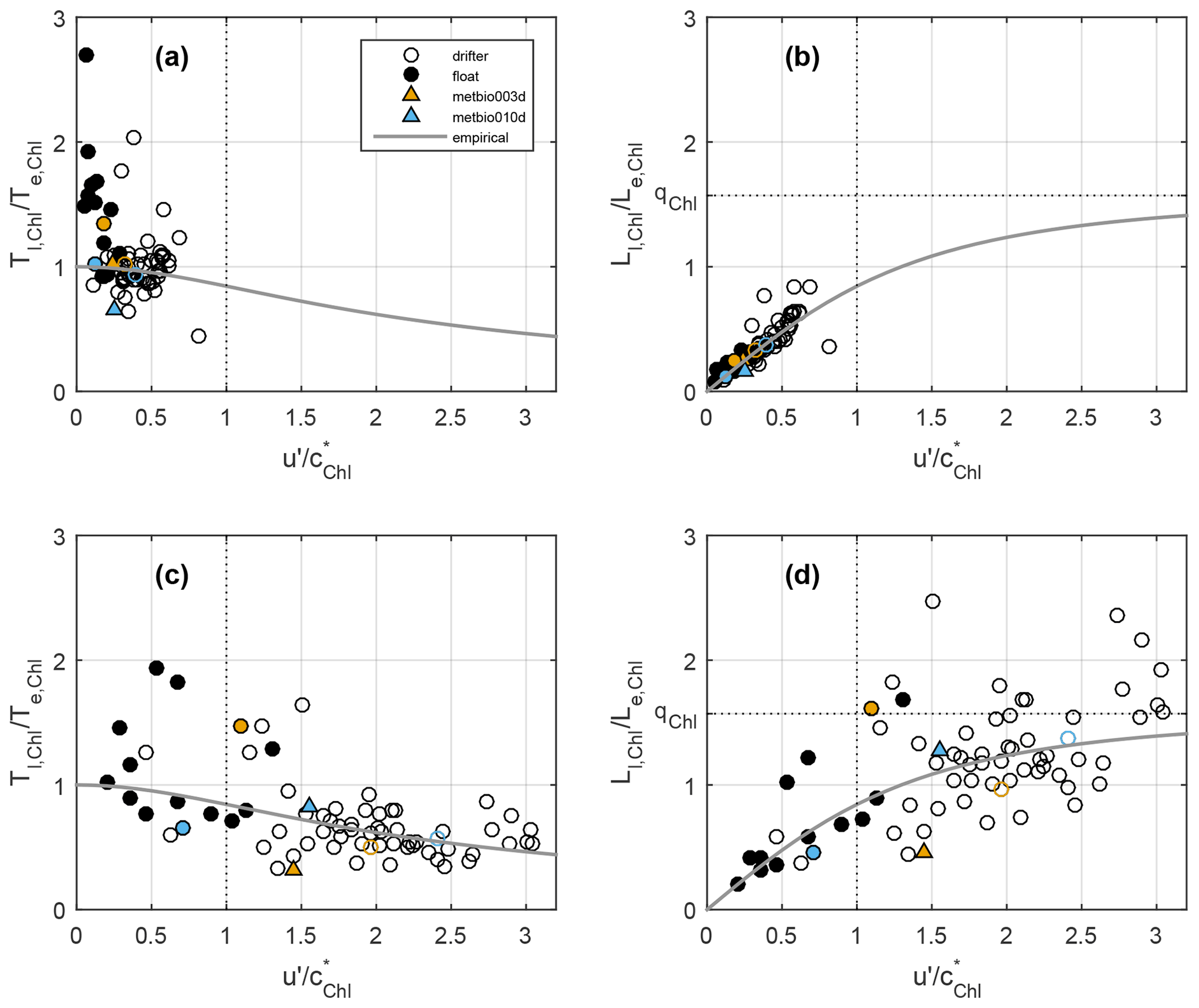
Figure D1The same as Fig. 6 but with float scales calculated by integrating Eq. (9) (space-composited ACF) instead of integrating Eq. (8) (individual segment ACF) and averaging over space.
In this paper, we analyse chlorophyll, as there is a history of geostatistical studies of that variable to build upon (e.g. Denman and Abbott, 1988, 1994; Doney et al., 2003; Glover et al., 2018; Eveleth et al., 2021). Chl is a complicated variable, containing a regionally (and seasonally) strong acclimation signal in addition to a biomass signal (Behrenfeld et al., 2005) that may imprint on our results. As a check, we evaluated Eulerian and Lagrangian timescales of phytoplankton carbon biomass (Cphyto) and compared them to timescales of Chl. Cphyto is derived from float (at 700 nm) or satellite-measured (at 443 nm) backscattering (following Table 2 in Graff et al., 2015, and assuming a spectral power law for backscattering of −0.78), anomalies are computed relative to equivalently constructed subtrahends as for Chl (as described in Sect. 3.3), and its ACF is integrated as for Chl (as described in Sect. 3.4). In general, Eulerian and Lagrangian timescales of Chl are longer than timescales of Cphyto in the subtropics (as defined by the −0.10 m mean absolute dynamic topography contour; Della Penna and Gaube, 2019), are shorter than timescales of Cphyto near coasts, and are approximately equal elsewhere, suggesting that there is a regional acclimation signal built into Chl that affects its timescales in certain regions of the ocean. However, importantly for this study, the relevant quantity is proportional to everywhere, meaning that, even if the biophysical drivers of variability in Chl and Cphyto vary regionally, the variables are sampled equivalently by a Lagrangian (or quasi-Lagrangian) observer, giving us confidence in our Chl-based results.
NAAMES float data are available from the University of Maine In-Situ Sound & Color Lab archive (http://misclab.umeoce.maine.edu/floats/, Haentjens and Boss, 2020). Sprof files for the non-NAAMES floats and prof files for the NAAMES floats (hydrographic variables only) are available from the IFREMER Argo Global Data Assembly Center (snapshot from February 2021; https://doi.org/10.17882/42182{#}81474, Argo, 2021). Altimetry data (product SEALEVEL_GLO_PHY_L4_REP_OBSERVATIONS_008_047; https://doi.org/10.48670/moi-00148) use the DT2018 processing (described in Taburet et al., 2019) which was superseded by the DT2021 version at the time of writing and is no longer accessible by URL; however, data can be de-archived by the Copernicus Marine Environmental Monitoring Service (https://marine.copernicus.eu/, Copernicus Marine Environment Monitoring Service, 2021) upon request. GlobColour data (variables CHL1 and BBP using “merged” sensors, L3m, daily binning, 25 km resolution, and the GSM algorithm) are from the R2019 processing available by web or FTP from ACRI-ST, France (https://hermes.acri.fr, ACRI GlobColour Team, 2020). Drifter data are the quality-controlled 6 h product available from the NOAA Global Drifter Program (https://doi.org/10.25921/7ntx-z961, Lumpkin and Centurioni, 2019), where we accessed the ASCII files on 14 September 2020.
DCM and SCD designed the study and DCM performed the analyses. ESB acquired and processed the NAAMES float data, DMG provided the Chl variogram parameters, and ADP helped develop the QPI. DCM prepared the manuscript with contributions from all co-authors.
The contact author has declared that none of the authors has any competing interests.
Publisher’s note: Copernicus Publications remains neutral with regard to jurisdictional claims in published maps and institutional affiliations.
We thank the two referees whose feedback improved this manuscript. Additional support was provided to Scott C. Doney and Darren C. McKee by the University of Virginia.
This research has been supported by the National Aeronautics and Space Administration, Earth Sciences Division (grant nos. 80NSSC18K0018 and 80NSSC20M0202).
This paper was edited by Ciavatta Stefano and reviewed by Bror Jonsson and one anonymous referee.
Abbott, M. R. and Letelier, R. M.: Decorrelation scales of chlorophyll as observed from bio-optical drifters in the California Current, Deep-Sea Res. Pt. II, 45, 1639–1667, https://doi.org/10.1016/S0967-0645(98)80011-8, 1998.
ACRI GlobColour Team: GlobColour version R2019, ACRI-ST [data set], https://hermes.acri.fr (last access: 28 January 2022), 2020.
Argo Data Management Team: Argo user's manual, Ifremer, https://doi.org/10.13155/29825, 2019.
Argo: Argo float data and metadata from Global Data Assembly Centre (Argo GDAC), SEANOE [data set], https://doi.org/10.17882/42182, 2021.
Ascani, F., Richards, K. J., Firing, E., Grant, S., Johnson, K. S., Jia, Y., Lukas, R., and Karl, D. M.: Physical and biological controls of nitrate concentrations in the upper subtropical North Pacific Ocean, Deep-Sea Res. Pt. II, 93, 119–134, https://doi.org/10.1016/j.dsr2.2013.01.034, 2013.
Behrenfeld, M. J. and Boss, E. S.: Student's tutorial on bloom hypotheses in the context of phytoplankton annual cycles, Glob. Change Biol., 24, 1–23, https://doi.org/10.1111/gcb.13858, 2018.
Behrenfeld, M. J., Boss, E. S., Siegel, D. A., and Shea, D. M.: Carbon-based ocean productivity and phytoplankton physiology from space, Global Biogeochem. Cy., 19, GB1006, https://doi.org/10.1029/2004GB002299, 2005.
Behrenfeld, M. J., Moore, R. H., Hostetler, C. A., Graff, J., Gaube, P., Russell, L. M., Chen, G., Doney, S. C., Giovannoni, S., Liu, H., Proctor, C., Bolaños, L. M., Baetge, N., Davie-Martin, C., Westberry, T. K., Bates, T. S., Bell, T. G., Bidle, K. D., Boss, E. S., Brooks, S. D., Cairns, B., Carlson, C., Halsey, K., Harvey, E. L., Hu, C., Karp-Boss, L., Kleb, M., Menden-Deuer, S., Morison, F., Quinn, P. K., Scarino, A. J., Anderson, B., Chowdhary, J., Crosbie, E., Ferrare, R., Hair, J. W., Hu, Y., Janz, S., Redemann, J., Saltzman, E., Shook, M., Siegel, D. A., Wisthaler, A., Martin, M. Y., and Ziemba, L.: The North Atlantic Aerosol and Marine Ecosystem Study (NAAMES): Science Motive and Mission Overview, Front. Mar. Sci., 6, 122, https://doi.org/10.3389/fmars.2019.00122, 2019.
Boss, E. S., Swift, D., Taylor, L., Brickley, P., Zaneveld, R., Riser, S., Perry, M. J., and Strutton, P. G.: Observations of pigment and particle distributions in the western North Atlantic from an autonomous float and ocean color satellite, Limnol. Oceanogr., 53, 2112–2122, 2008.
Briggs, N., Gudmundsson, K., Cetiníc, I., D'Asaro, E., Rehm, E., Lee, C., and Perry, M. J.: A multi-method autonomous assessment of primary productivity and export efficiency in the springtime North Atlantic, Biogeosciences, 15, 4515–4532, https://doi.org/10.5194/bg-15-4515-2018, 2018.
Chai, F., Johnson, K. S., Claustre, H., Xing, X., Wang, Y., Boss, E. S., Riser, S., Fennel, K., Schofield, O., and Sutton, A.: Monitoring ocean biogeochemistry with autonomous platforms, Nat. Rev. Earth Environ., 1, 315–326, https://doi.org/10.1038/s43017-020-0053-y, 2020.
Chelton, D. B., Schlax, M. G., and Samelson, R. M.: Global observations of nonlinear mesoscale eddies, Prog. Oceanogr., 91, 167–216, https://doi.org/10.1016/j.pocean.2011.01.002, 2011.
Chenillat, F., Blanke, B., Grima, N., Franks, P. J. S., Capet, X., and Rivière, P.: Quantifying tracer dynamics in moving fluids: a combined Eulerian-Lagrangian approach, Front. Environ. Sci., 3, 43, https://doi.org/10.3389/fenvs.2015.00043, 2015.
Claustre, H., Bishop, J., Boss, E. S., Stewart, B., Berthon, J.-F., Coatanoan, C., Johnson, K., Lotiker, A., Ulloa, O., Perry, M. J., D'Ortenzio, F., Hembise Fanton D'Andon, O., and Uitz, J.: Bio-optical profiling floats as new observational tools for biogeochemical and ecosystem studies, in: Proceedings of the “OceanObs'09: Sustained Ocean Observations and Information for Society” Conference, Venice, Italy, 21–25 September 2009, edited by: Hall, J., Harrison, D. E., and Stammer, D., ESA, WPP-306, 1–7, https://doi.org/10.5270/OceanObs09.cwp.17, 2010.
Copernicus Marine Environment Monitoring Service: Global ocean gridded L4 sea surface heights and derived variables reprocessed (1993–ongoing), Copernicus Marine Environment Monitoring Service [data set], https://doi.org/10.48670/moi-00148, 2021.
Global ocean gridded L4 sea surface heights and derived variables reprocessed (1993–ongoing), Copernicus Marine Environment Monitoring Service [data set], https://doi.org/10.48670/moi-00148, 2021.
Della Penna, A. and Gaube, P.: Overview of (sub)mesoscale ocean dynamics for the NAAMES field program, Front. Mar. Sci., 6, 384, https://doi.org/10.3389/fmars.2019.00384, 2019.
Della Penna, A., De Monte, S., Kestenare, E., Guinet, C., and d'Ovidio, F.: Quasi-planktonic behavior of foraging top marine predators, Sci. Rep., 5, 18063, https://doi.org/10.1038/srep18063, 2015.
Denman, K. L. and Abbott, M. R.: Time evolution of surface chlorophyll patterns from cross-spectrum analysis of satellite color images, J. Geophys. Res., 93, 6789–6798, https://doi.org/10.1029/JC093iC06p06789, 1988.
Denman, K. L. and Abbott, M. R.: Time scales of pattern evolution from cross-spectrum analysis of advanced very high resolution radiometer and coastal zone color scanner imagery, J. Geophys. Res., 99, 7433–7442, 1994.
Doney, S. C., Glover, D. M., McCue, S. J., and Fuentes, M.: Mesoscale variability of sea-viewing wide field-of-view sensor (SeaWIFS) satellite ocean color: Global patterns and spatial scales, J. Geophys. Res., 108, 3024, https://doi.org/10.1029/2001JC000843, 2003.
d'Ovidio, F., Monte, S. D., Penna, A. D., Cotté, C., and Guinet, C.: Ecological implications of eddy retention in the open ocean: a Lagrangian approach, J. Phys. Math. Theor., 46, 254023, https://doi.org/10.1088/1751-8113/46/25/254023, 2013.
Eveleth, R., Glover, D. M., Long, M. C., Lima, I. D., Chase, A. P., and Doney, S. C.: Assessing the Skill of a High-Resolution Marine Biophysical Model Using Geostatistical Analysis of Mesoscale Ocean Chlorophyll Variability From Field Observations and Remote Sensing, Front. Mar. Sci., 8, 1–10, https://doi.org/10.3389/fmars.2021.612764, 2021.
Gaube, P., McGillicuddy, D. J., Chelton, D. B., Behrenfeld, M. J., and Strutton, P. G.: Regional variations in the influence of mesoscale eddies on near-surface chlorophyll, J. Geophys. Res.-Ocean., 119, 8195–8220, https://doi.org/10.1002/2014JC010111, 2014.
Glover, D. M., Jenkins, W. J., and Doney, S. C.: Modeling Methods for Marine Science, Cambridge University Press, Cambridge, UK, 592 pp., ISBN: 978-0-521-86783-2, 2011.
Glover, D. M., Doney, S. C., Oestreich, W. K., and Tullo, A. W.: Geostatistical analysis of mesoscale spatial variability and error in SeaWiFS and MODIS/Aqua global ocean color data, J. Geophys. Res.-Ocean., 123, 22–39, https://doi.org/10.1002/2017JC013023, 2018.
Gordon, H. and McCluney, W.: Estimation of the depth of sunlight penetration in the sea for remote sensing, Appl. Opt., 14, 413–416, https://doi.org/10.1364/AO.14.000413, 1975.
Graff, J. R. and Behrenfeld, M. J.: Photoacclimation responses in Subarctic Atlantic Phytoplankton following a natural mixing-restratification event, Front. Mar. Sci., 5, 1–11, https://doi.org/10.3389/fmars.2018.00209, 2018.
Graff, J. R., Westberry, T. K., Milligan, A. J., Brown, M. B., Dall'Olmo, G., van Dongen-Vogels, V., Reifel, K. M., and Behrenfeld, M. J.: Analytical phytoplankton carbon measurements spanning diverse ecosystems, Deep-Sea Res. Pt. I, 102, 16–25, https://doi.org/10.1016/j.dsr.2015.04.006, 2015.
Gruber, N., Doney, S. C., Emerson, S., Gilbert, D., Kobayashi, T., Körtzinger, A., Johnson, G. C., Johnson, K. S., Riser, S., and Ulloa, O.: Adding oxygen to Argo: Developing a global in-situ observatory for ocean deoxygenation and biogeochemistry, in: Proceedings of the “OceanObs'09: Sustained Ocean Observations and Information for Society” Conference, Venice, Italy, 21–25 September 2009., edited by: Hall, J., Harrison, D. E., and Stammer, D., ESA, WPP-306, 1–10, https://doi.org/10.5270/OceanObs09.cwp.39, 2010.
Haentjens, N. and Boss, E.: Bio-Argo floats in the study area of NAAMES [data set], http://misclab.umeoce.maine.edu/floats/, last access: 30 April 2020
Jönsson, B. F. and Salisbury, J. E.: Episodicity in phytoplankton dynamics in a coastal region, Geophys. Res. Lett., 43, 5821–5828, https://doi.org/10.1002/2016GL068683, 2016.
Jönsson, B. F., Salisbury, J. E., and Mahadevan, A.: Extending the use and interpretation of ocean satellite data using Lagrangian modelling, Int. J. Remote Sens., 30, 3331–3341, https://doi.org/10.1080/01431160802558758, 2009.
Jönsson, B. F., Salisbury, J. E., and Mahadevan, A.: Large variability in continental shelf production of phytoplankton carbon revealed by satellite, Biogeosciences, 8, 1213–1223, https://doi.org/10.5194/bg-8-1213-2011, 2011.
Klein, P., Isern-Fontanet, J., Lapeyre, G., Roullet, G., Danioux, E., Chapron, B., Le Gentil, S., and Sasaki, H.: Diagnosis of vertical velocities in the upper ocean from high resolution sea surface height, Geophys. Res. Lett., 36, L12603, https://doi.org/10.1029/2009GL038359, 2009.
Kuhn, A. M., Dutkiewicz, S., Jahn, O., Clayton, S., Rynearson, T. A., Mazloff, M. R., and Barton, A. D.: Temporal and spatial scales of correlation in marine phytoplankton communities, J. Geophys. Res.-Oceans, 124, 9417–9438, https://doi.org/10.1029/2019JC015331, 2019.
LaCasce, J. H.: Statistics from Lagrangian observations, Prog. Oceanogr., 77, 1–29, https://doi.org/10.1016/j.pocean.2008.02.002, 2008.
Lacour, L., Ardyna, M., Stec, K. F., Claustre, H., Prieur, L., Poteau, A., Ribera D'Alcala, M., and Iudicone, D.: Unexpected winter phytoplankton blooms in the North Atlantic subpolar gyre, Nat. Geosci., 10, 836–839, https://doi.org/10.1038/NGEO3035, 2017.
Lapeyre, G. and Klein, P.: Dynamics of the upper oceanic layers in terms of surface quasigeostrophy theory, J. Phys. Oceanogr., 36, 165–176, https://doi.org/10.1175/JPO2840.1, 2006.
Lehahn, Y., d'Ovidio, F., Lévy, M., and Heifetz, E.: Stirring of the northeast Atlantic spring bloom: A Lagrangian analysis based on multisatellite data., J. Geophys. Res., 112, 1–15, https://doi.org/10.1029/2006JC003927, 2007.
Lehahn, Y., Koren, I., Sharoni, S., d'Ovidio, F., Vardi, A., and Boss, E. S.: Dispersion/dilution enhances phytoplankton blooms in low-nutrient waters, Nat. Commun., 8, 1–8, https://doi.org/10.1038/ncomms14868, 2017.
Lévy, M., Jahn, O., Dutkiewicz, S., and Follows, M. J.: Phytoplankton diversity and community structure affected by oceanic dispersal and mesoscale turbulence, Limnol. Oceanogr. Fluid. Environ., 4, 67–84, https://doi.org/10.1215/21573689-2768549, 2014.
Lévy, M., Franks, P. J. S., and Smith, K. S.: The role of submesoscale currents in structuring marine ecosystems, Nat. Commun., 9, 4758, https://doi.org/10.1038/s41467-018-07059-3, 2018.
Llort, J., Langlais, C., Matear, R., Moreau, S., Lenton, A., and Strutton, P. G.: Evaluating southern ocean carbon eddy-pump from biogeochemical-Argo floats, J. Geophys. Res.-Ocean., 123, 971–984, https://doi.org/10.1002/2017JC012861, 2018.
Lumpkin, R. and Centurioni, L.: Global Drifter Program quality-controlled 6-hour interpolated data from ocean surface drifting buoys, NOAA National Centers for Environmental Information [data set], https://doi.org/10.25921/7ntx-z961, 2019.
Lumpkin, R., Treguier, A.-M., and Speer, K.: Lagrangian eddy scales in the Northern Atlantic Ocean, J. Phys. Oceanogr., 32, 2425–2440, 2002.
Mahadevan, A.: The Impact of Submesoscale Physics on Primary Productivity of Plankton, Annu. Rev. Mar. Sci., 8, 161–184, https://doi.org/10.1146/annurev-marine-010814-015912, 2016.
Middleton, J. F.: Drifter spectra and diffusivities, J. Mar. Res., 43, 37–55, 1985.
Morel, A., Hout, Y., Gentili, B., Werdell, P. J., Hooker, S. B., and Franz, B. A.: Examining the consistency of products derived from various ocean color sensors in open ocean (Case 1) waters in the perspective of a multi-sensor approach, Remote Sens. Environ., 111, 69–88, https://doi.org/10.1016/j.rse.2007.03.012, 2007.
Philip, J. R.: Relation between Eulerian and Lagrangian Statistics, Phys. Fluids Suppl., 10, 69–71, https://doi.org/10.1063/1.1762507, 1967.
Schmechtig, C., Claustre, H., Poteau, A., and D'Ortenzio, F.: Bio-Argo quality control manual for Chlorophyll-A concentration Version 1.1, Argo Data Management, 1–16, https://doi.org/10.13155/35385, 2018.
Smith, K. S.: The geography of linear baroclinic instability in Earth's oceans, J. Mar. Res., 65, 655–683, https://doi.org/10.1357/002224007783649484, 2007.
Smith, K. S. and Ferrari, R.: The Production and Dissipation of Compensated Thermohaline Variance by Mesoscale Stirring, J. Phys. Oceanogr., 39, 2477–2501, https://doi.org/10.1175/2009JPO4103.1, 2009.
Sudre, J. and Morrow, R. A.: Global surface currents: a high-resolution product for investigating ocean dynamics, Ocean Dynam., 58, 101–118, https://doi.org/10.1007/s10236-008-0134-9, 2008.
Taburet, G., Sanchez-Roman, A., Ballarotta, M., Pujol, M.-I., Legeais, J.-F., Fournier, F., Faugere, Y., and Dibarboure, G.: DUACS DT2018: 25 years of reprocessed sea level altimetry products, Ocean Sci., 15, 1207–1224, https://doi.org/10.5194/os-15-1207-2019, 2019.
Taylor, G. I.: Diffusion by continuous movements, Proc. Math. Soc. Lond., 20, 196–212, 1922.
Taylor, G. I.: The spectrum of turbulence, Proc. R. Soc. Math. Phys. Eng. Sci., 164, 476–490, https://doi.org/10.1098/rspa.1938.0032, 1938.
van Sebille, E., Griffies, S. M., Abernathey, R., Adams, T. P., Berloff, P., Biastoch, A., Blanke, B., Chassignet, E. P., Cheng, Y., Cotter, C. J., Deleersnijder, E., Döös, K., Drake, H. F., Drijfhout, S., Gary, S. F., Heemink, A. W., Kjellsson, J., Koszalka, I. M., Lange, M., Lique, C., MacGilchrist, G. A., Marsh, R., Mayorga Adame, C. G., McAdam, R., Nencioli, F., Paris, C. B., Piggott, M. D., Polton, J. A., Rühs, S., Shah, S. H. A. M., Thomas, M. D., Wang, J., Wolfram, P. J., Zanna, L., and Zika, J. D.: Lagrangian ocean analysis: Fundamentals and practices, Ocean Model., 121, 49–75, https://doi.org/10.1016/j.ocemod.2017.11.008, 2018.
Xing, X., Claustre, H., Blain, S., D'Ortenzio, F., Antoine, D., Ras, J., and Guinet, C.: Quenching correction for in vivo chlorophyll fluorescence acquired by autonomous platforms: A case study with instrumented elephant seals in the Kerguelen region (Southern Ocean), Limnol. Oceanogr. Methods, 10, 483–495, 2012.
Yang, B.: Seasonal relationship between net primary and net community production in the subtropical gyres: Insights from satellite and Argo profiling float measurements, Geophys. Res. Lett., 48, e2021GL093837, https://doi.org/10.1029/2021GL093837, 2021.
Yang, B., Boss, E. S., Haëntjens, N., Long, M. C., Behrenfeld, M. J., Eveleth, R., and Doney, S. C.: Controls on the North Atlantic Phytoplankton Bloom: Insights from Profiling Float Measurements, Front. Mar. Sci., 7, 139, https://doi.org/10.3389/fmars.2020.00139, 2020.
Zaiss, J., Boyd, P. W., Doney, S. C., Havenhand, J. N., and Levine, N. M.: Impact of Lagrangian Sea Surface Temperature Variability on Southern Ocean Phytoplankton Community Growth Rates, Global Biogeochem. Cy., 35, e2020GB006880, https://doi.org/10.1029/2020GB006880, 2021.
Zhang, Z., Qiu, B., Klein, P., and Travis, S.: The influence of geostrophic strain on oceanic ageostrophic motion and surface chlorophyll, Nat. Commun., 10, 1–11, https://doi.org/10.1038/s41467-019-10883-w, 2019.