Reconstruction of global surface ocean pCO₂ using region-specific predictors based on a stepwise FFNN regression algorithm

Various machine learning methods were attempted in the global mapping of surface ocean partial pressure of CO₂ (pCO₂) to reduce the uncertainty of the global ocean CO₂ sink estimate due to undersampling of pCO₂. In previous research, the predictors of pCO₂ were usually selected empirically based on theoretic drivers of surface ocean pCO₂, and the same combination of predictors was applied in all areas except where there was a lack of coverage. However, the differences between the drivers of surface ocean pCO₂ in different regions were not considered. In this work, we combined the stepwise regression algorithm and a feed-forward neural network (FFNN) to select predictors of pCO₂ based on the mean absolute error in each of the 11 biogeochemical provinces defined by the self-organizing map (SOM) method. Based on the predictors selected, a monthly global 1^∘ × 1^∘ surface ocean pCO₂ product from January 1992 to August 2019 was constructed. Validation of different combinations of predictors based on the Surface Ocean CO₂ Atlas (SOCAT) dataset version 2020 and independent observations from time series stations was carried out. The prediction of pCO₂ based on region-specific predictors selected by the stepwise FFNN algorithm was more precise than that based on predictors from previous research. Applying the FFNN size-improving algorithm in each province decreased the mean absolute error (MAE) of the global estimate to 11.32 µatm and the root mean square error (RMSE) to 17.99 µatm. The script file of the stepwise FFNN algorithm and pCO₂ product are distributed through the Institute of Oceanology of the Chinese Academy of Sciences Marine Science Data Center (IOCAS, https://doi.org/10.12157/iocas.2021.0022, Zhong, 2021.

1 Introduction

As a net sink for atmospheric CO₂, global oceans have removed about one-third of anthropogenic CO₂ since the beginning of the industrial revolution (Sabine et al., 2004; Friedlingstein et al., 2019). However, the global ocean sea–air CO₂ flux averaged between 2001–2015 varies from −1.55 to −1.74 Pg C yr⁻¹ with a maximum difference in individual years of nearly 0.6 Pg C yr⁻¹, depending on the surface ocean partial pressure of the CO₂ (pCO₂) product. These differences largely stem from differences in pCO₂ estimates across the products (Rödenbeck et al., 2014; Iida et al., 2015; Landschützer et al., 2014; Denvil-Sommer et al., 2019). The magnitude and direction of the flux are primarily set by the air–sea pCO₂ difference. Surface water pCO₂ greater than the overlying air indicates CO₂ is released from the ocean to the air. Conversely, absorption of CO₂ by oceans happens when the pCO₂ of the surface water is lower than the overlying air. The ocean in these two scenarios is known as the oceanic carbon source and oceanic carbon sink, respectively.

Sparse and uneven observations of surface ocean pCO₂ in time and space have severely limited the understanding of interannual variability of oceanic carbon sink, and research based on different methods were carried out to break this barrier. In earlier studies, traditional unitary and multiple regression methods between surface ocean pCO₂ and its drivers were attempted in the mapping of surface ocean pCO₂, which were limited in specific regions and sometimes even in particular seasons with a relatively high root mean square error (RMSE; Sarma et al., 2006; Takahashi et al., 2006; Shadwick et al., 2010; Chen et al., 2011; Marrec et al., 2015). Advances in artificial neural networks and other machine learning algorithms, such as the feed-forward neural network (FFNN) method (Zeng et al., 2014, 2015; Moussa et al., 2016; Denvil-Sommer et al., 2019) and self-organization mapping (SOM) method (Friedrich and Oschlies, 2009; Telszewski et al., 2009; Hales et al., 2012; Nakaoka et al., 2013), significantly reduced the bias in interpolation based on relationships between surface ocean pCO₂ and its drivers. In addition, finding better predictors or combining SOM with other neural networks was also attempted to decrease the pCO₂ predicting error further (Hales et al., 2012; Nakaoka et al., 2013; Landschützer et al., 2014; Chen et al., 2019; Denvil-Sommer et al., 2019; Zhong et al., 2020; Wang et al., 2021). However, the selection of predictors in the surface ocean pCO₂ mapping was more empirical, focusing on the theoretical drivers of the pCO₂ and its variation. Sea surface temperature and salinity, related to the solubility of CO₂ in seawater, are considered as the most important and used in almost all related studies (Landschützer et al., 2013; Nakaoka et al., 2013; Moussa et al., 2016; Laruelle et al., 2017; Zeng et al., 2017; Denvil-Sommer et al., 2019). Similarly, the chlorophyll a concentration, which is related to the phytoplankton uptake of CO₂, is also widely used (Nakaoka et al., 2013; Landschützer et al., 2014; Laruelle et al., 2017; Zeng et al., 2017; Denvil-Sommer et al., 2019). One more predictor, mixed layer depth, frequently appears in associated studies as a proxy related to the vertical transport of dissolved carbon (Telszewski et al., 2009; Nakaoka et al., 2013; Landschützer et al., 2014; Zeng et al., 2017; Denvil-Sommer et al., 2019). In addition, sampling information, such as latitude and longitude (Friedrich and Oschlies, 2009; Jo et al., 2012; Zeng et al., 2015, 2017; Denvil-Sommer et al., 2019; Gregor et al., 2019) and sampling time (Friedrich and Oschlies, 2009; Zeng et al., 2015), has been used as a predictor. In recent research, the dry air mixing ratio of atmospheric CO₂ (xCO₂), related to the CO₂ level in the air, was also used to predict surface ocean pCO₂ (Landschützer et al., 2014; Denvil-Sommer et al., 2019). The sea surface height, which was considered effective in improving the spatial pattern and the accuracy of surface ocean pCO₂ mapping at the basin and regional scales, and the monthly anomalies of the most widely used predictors mentioned above, were used by Denvil-Sommer et al. (2019). In research focusing on the surface ocean pCO₂ mapping of coastal areas, bathymetry, sea ice, and wind speed were also used as predictors (Laruelle et al., 2017). In each of these research studies, the same combination of predictors was applied in all global ocean areas, although the global ocean was divided into several biogeochemical provinces in some of the research. However, the predictor that plays a vital role in the surface ocean pCO₂ reconstruction at one region may not be a good predictor of surface ocean pCO₂ in the other regions due to complex and variable drivers. Nevertheless, no widely recognized methods for judging the importance of each predictor in the surface ocean pCO₂ mapping are available yet. Thus, we attempted to construct a stepwise FFNN algorithm to rank the importance of predictors and figure out the optimal combination in each biogeochemical province defined by SOM for decreasing the prediction errors in the surface ocean pCO₂ mapping.

2 Methodology

2.1 Data

The surface ocean fugacity of CO₂ (fCO₂) observation data from the Surface Ocean CO₂ Atlas fCO₂ dataset version 2020 (SOCATv2020; Bakker et al., 2016) was used to construct the non-linear relationship between surface ocean pCO₂ and predictors. The conversion between fCO₂ and pCO₂ followed the formula (Körtzinger, 1999)

$$\begin{array}{}\text{(1)}& f{\mathrm{CO}}_{\mathrm{2}}=p{\mathrm{CO}}_{\mathrm{2}}\cdot \exp \left(P\cdot {\displaystyle \frac{B+\mathrm{2}\mathit{\delta }}{RT}}\right),\end{array}$$

where fCO₂ and pCO₂ are in micro-atmospheres (µatm), P is the total atmospheric surface pressure (Pa) using the National Centers for Environmental Prediction (NCEP) monthly mean sea level pressure product (Dee et al., 2011), and T is the absolute temperature (K). R is the gas constant (8.314 $\mathrm{J}{\mathrm{K}}^{-\mathrm{1}}{\mathrm{mol}}^{-\mathrm{1}}$). Parameters B (m³ mol⁻¹) and δ (m³ mol⁻¹) are both viral coefficients (Weiss, 1974).

Table 1 Predictors and corresponding data products.

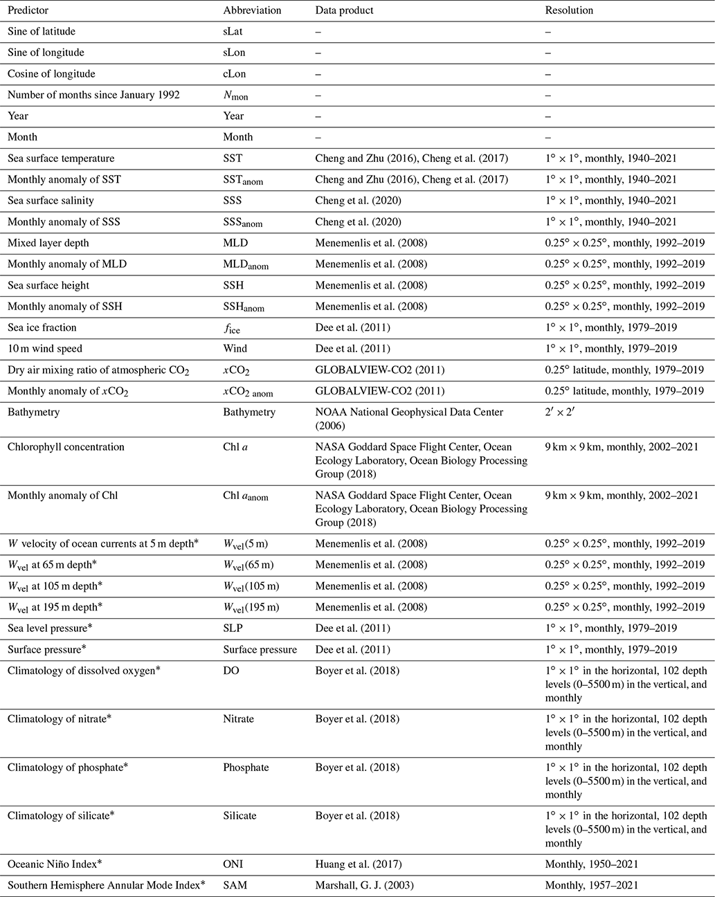
Predictors with the ^∗ label were here for the first time included in the pCO₂ mapping. All data products retrieved at resolutions higher than 1^∘ × 1^∘ were downscaled to 1^∘ × 1^∘ resolution.

In this work, 33 predictors were used (Table 1), where 21 were chosen from previous research of surface ocean pCO₂ reconstruction based on machine learning methods. In addition, 12 predictors that were only used in similar previous research focused on the mapping of total alkalinity or dissolved inorganic carbon (Broullón et al., 2019; Broullón et al., 2020), or were possibly related to the driver of surface ocean pCO₂ and its variability, were selected for testing (predictors labeled with * in Table 1). Most of these products were retrieved at 1^∘ × 1^∘ resolution. Some products retrieved at higher resolution were downscaled to 1^∘ × 1^∘ resolution by taking the average of all values in each 1^∘ × 1^∘ grid.

2.2 Biogeochemical provinces defined by the self-organizing map

For applying a different combination of predictors in regions based on the differences in the dominated drivers of pCO₂ and its variability, the global ocean was divided into a set of biogeochemical provinces using a self-organizing map (SOM) method. The monthly climatology of temperature, salinity, mixed layer depth, sea surface height, nitrate, phosphate, silicate, and dissolved oxygen and pCO₂ climatology from Landschützer et al. (2020) were put into a 3-by-4 SOM network to generate 12 biogeochemical provinces, where the monthly climatology data in all 12 months were put into one SOM network to generate one discrete set of biogeochemical provinces. Provinces with less than 10 pixels and less than 1000 SOCAT observations were defined as discrete small “island” provinces and then merged with nearest provinces. The provinces covering areas separated by land were further divided artificially. For example, the province covering the northern subtropical Pacific and the province covering the northern subtropical Atlantic was set as one province in the original output of SOM, but it was mainly separated by the North American continent. So, we divided the province into two new provinces. The final version includes 11 biogeochemical provinces. In this study, the coastal area was not involved, and the boundary was defined as 200 m depth. In addition, the pCO₂ mapping based on SOM-defined provinces tends to be less smooth near the border of different biogeochemical provinces, with an obvious borderline appearing. However, applying different predictors may make this problem worse. To obtain a smoother distribution, we defined the area within five 1 × 1 grids of province boundaries as a “boundary area”. Samples in the boundary area will be used as training samples in all adjacent provinces (Fig. S1 in the Supplement). However, this definition does not change the actual spatial coverage of each province, only bringing more training samples near the province boundary.

2.3 Stepwise FFNN algorithm

For finding a better combination of pCO₂ predictors, a stepwise FFNN algorithm was constructed. The FFNN comprises four parts: input, hidden, summation, and output layers (Fig. 1). The input layer is designed to pass the inputs to the hidden layer, and the number of neurons is equal to the dimensions of the input matrix p. The hidden layer includes 25 neurons in the FFNN model, with a tan-sigmoid function as the transfer function. The input p is multiplied by a matrix of weights (w₁ in Fig. 1), and the inner product between the result and a bias matrix (b₁ in Fig. 1) is calculated as the input of the transfer function in the first hidden layer. In the summation layer, the transfer function f₂ is a linear function. The output of the hidden layer is multiplied by another matrix of weights and summed. All bias and weights matrixes were randomly assigned at the beginning of FFNN training. The randomly assigned bias and weights matrixes, the number of training samples, and the sort order of training samples in the input matrix p define where the FFNN starts training in errors space. The practice of FFNN changes when these conditions change. Here we fixed the training samples and set one constant random number stream in MATLAB to ensure that the difference between the MAE based on different predictors entirely stems from the predictor differences. The random number was randomly chosen. When using different random number streams, several predictors at the end of the output list of the stepwise FFNN algorithm differed. However, the leading predictors were consistent, and the different predictors were also related. The fixed random number makes all networks using different predictors start training from the same point in the error space when comparing the performance of each predictor.

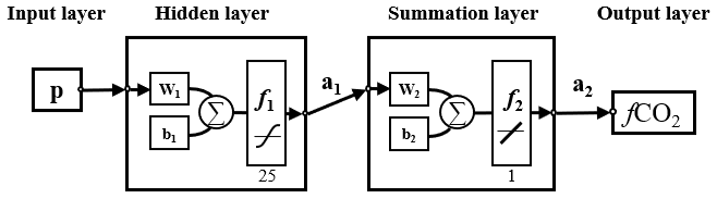
Figure 1 Structure of the feed-forward neural network. w: weighted matrix; b: bias matrix; ∑: sum; f₁: tan-sigmoid transfer function; f₂: linear function; a: output matrix.

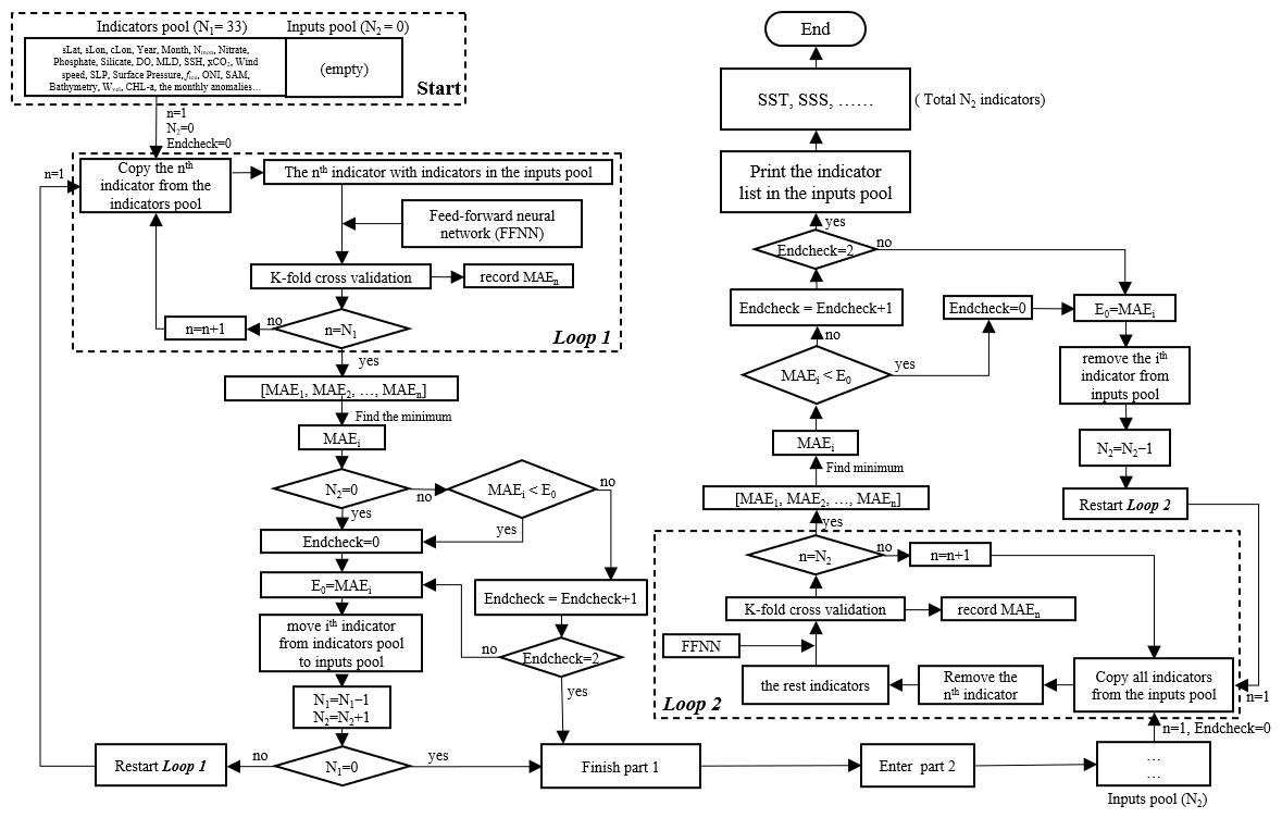
Figure 2 The procedure of the stepwise FFNN algorithm. The flowchart follows an order of top left–bottom left–bottom right–top right. The meaning of Predictors pool: store all predictors waiting to be tested; Inputs pool: store predictors that were temporally considered as good predictors; Loop 1 and Loop 2: calculate the MAE when each predictor was added or removed; Selection step: add good predictors to the Inputs pool; Removal step: remove predictors from the Inputs pool if removing leads to MAE decrease; Determine step: check if the process reaches end condition. N₁ and N₂: number of predictors in the Predictors pool and Inputs pool, respectively; E₀: lowest MAE in the last iteration of Loop 1 or Loop 2; Endcheck: the number of iterations that E₀ continuously increased.

In the stepwise part, predictors of pCO₂ are going to be added and removed one by one, and which predictors will be finally used in pCO₂ predicting is determined according to the real-time change of predicting error. The mean absolute error (MAE), calculated using a K-fold cross validation method, was used to estimate the performance of each predictor in the FFNN predicting. Although the RMSE was widely used for the validation of machine learning methods, compared to the MAE, the RMSE was more sensitive to a few extreme samples, which generally deviated far from the FFNN predicting values, resulting in a considerable discrepancy between the FFNN outputs and pCO₂ observations by sometimes up to hundreds of micro-atmospheres. A higher weight might be put on these few extreme samples than other samples in the predictor selection if the performance of each predictor was estimated by RMSE in the stepwise FFNN algorithm. To avoid the higher weight on these few extreme samples, the MAE was used instead for the internal performance loss function in the stepwise FFNN algorithm. The basic principle of the stepwise FFNN algorithm was adding each predictor from a set of predictors into the inputs of FFNN and removing each redundant predictor from the inputs successively to reduce the MAE in the fastest way, until no decrease in the MAE appeared (Fig. 2), and where the predictor having no contribution to the reducing of prediction error was considered as redundant.

At the beginning of the stepwise FFNN algorithm, all available predictors were put into a matrix, referred to as the Predictors pool (Start in Fig. 2). Each row represents one predictor, and each column represents one SOCAT sample. In this work, we collected 33 predictors for the test, that is, the Predictors pool matrix has 33 rows. Meanwhile, a matrix referred to as Inputs pool (Start in Fig. 2) was set up to store predictors with good performance, where good performance means that adding these predictors can significantly decrease the MAE between SOCAT pCO₂ measurements and FFNN pCO₂ predictions. Then a loop of K-fold validation test ran out to calculate the MAE when predicting pCO₂ by each predictor in the Predictors pool in the first step (Loop 1 in Fig. 2). Thus 33 MAE values were obtained in total, and the minimum was recorded as E₀. The predictor corresponding to the minimum MAE value was moved from the Predictors pool to the Inputs pool (Selection step in Fig. 2). After that, the Loop 1 restarted, i.e., the second step started with one predictor removed to the inputs pool and the remaining 32 predictors waiting to be tested. Then, the pCO₂ was predicted using each of the rest 32 predictors in the predictors pool with the addition of all predictors in the inputs pool, and 32 MAE values were calculated out. If the MAE in the lowest situation, represented by the MAE_i, decreased compared to the E₀, the ith predictor was considered a good predictor and moved from the predictors pool to the inputs pool. Then the value of E₀ was replaced by the MAE_i (Selection step in Fig. 2). Part 1, including Loop 1, Selection step, and Determine step 1 in Fig. 2, was repeated until no predictor was left in the Predictors pool or no decrease of E₀ could be found regardless of which two predictors were added in the next two steps. At this time, part 1 of the stepwise FFNN algorithm finished, and all predictors left in the Predictors pool were considered redundant. The second part ran in the opposite way in that the predictors were removed from the Inputs pool one by one to decrease E₀ the fastest (Loop 2 in Fig. 2). The second part was used to remove the predictor that could be represented by other predictors in the inputs pool (Removal step in Fig. 2) and finished in the similar condition that no significant decrease could be found regardless of which predictor was removed in the next two steps (Determine step 2 in Fig. 2).

2.4 pCO₂ product

The dataset of predictors, except for chl a, start in 1992 or earlier, while the chl a data range from August 2002 to the present. In each province, the stepwise FFNN algorithm was run once, first based on all samples covered by the chl a data; secondly, the algorithm was run based on samples and all predictors except chl a and chl a_anom in the year that chl a gridded data were not available. The pCO₂ mapping in the year that chl a gridded data were not available was carried out based on the predictors selected in the second run. Then the final product was built based on two FFNNs: one trained for the period from August 2002 to August 2019 using one predictor set including chl a or chl a_anom, and the second one for the period from January 1992 to July 2002 using the second predictor set without chl a and chl a_anom. Although the performance may improve with the number of neurons increasing, the influence of the number of neurons on the performance of FFNN pCO₂ prediction remains unclear. To further decrease the predicting error between FFNN outputs and SOCAT measurements, the number of neurons was improved by an error test in each province. The number of neurons increased from 5 to 300 (the increment was five during 5–50 and ten during 50–100 and fifty during 100–300). Then the corresponding MAE values of each size were recorded, and the number of neurons with the lowest MAE was applied. This test avoided the appearance of insufficient learning capacity for complex nonlinear relationships due to too few neurons and the overfitting problem due to too many neurons. Finally, based on the predictors selected by the stepwise FFNN algorithm and improved FFNN size, a monthly global 1^∘ × 1^∘ surface ocean pCO₂ product from January 1992 to August 2019 was constructed.

Table 2 Validation group using different predictors.

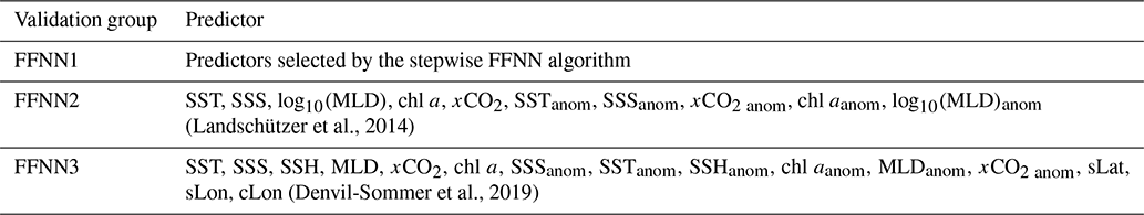
The FFNN performance of three groups with different predictors of pCO₂ were compared to test the result of stepwise FFNN algorithm. Predictors in group FFNN1 were selected using the stepwise FFNN algorithm, and predictors in group FFNN2 were selected from Landschützer et al. (2014), and in group FFNN3 from Denvil-Sommer et al. (2019).

2.5 Validation

To better estimate the predicting error of FFNN, the MAE and the RMSE, which were widely used in previous research, were calculated using a K-fold cross validation method. To avoid overfitting caused by a lack of independence between the training and testing samples, we put the SOCAT samples in chronological order and then divided them into the group of years (Fig. 1; Gregor et al., 2019). In this paper, the value of K was set as 4. Thus, among every four neighboring years, three group samples were used to train the FFNN model, and the rest were used for testing. A total of four iterations were carried out, where the testing year changed in each iteration. After the four iterations finished, all samples were used for testing only once, and the MAE and RMSE between FFNN output and the testing samples were calculated. The performance of the predictor selection algorithm was estimated by comparing the MAE and RMSE results of the FFNN based on predictors selected by the stepwise FFNN algorithm with the result based on predictors used in previous research in each biogeochemical province (Table 2). All validation groups were applied with the same FFNN and same samples from SOCAT, with the only differences being in the predictors. The same K-fold validation procedure was applied for three validation groups based on different pCO₂ predictors. Thus, three results were generated to estimate whether the stepwise FFNN algorithm can effectively find a better combination of pCO₂ predictors. Finally, the pCO₂ data generated in all validation groups were further compared with the completely independent observations from the Hawaii Ocean Time-series (HOT, 22^∘45^′ N, 158^∘00^′ W, since October 1988; Dore et al., 2009), Bermuda Atlantic Time-series Study (BATS, 31^∘50^′ N, 64^∘10^′ W, since October 1988; Bates, 2007) and The European Station for Time Series in the Ocean Canary Islands (ESTOC, 29^∘10^′ N, 15^∘30^′ W, from 1995 to 2009; González-Dávila and Santana-Casiano, 2012) stations. The pCO₂ at HOT and BATS were estimated from total alkalinity (TA) and dissolved inorganic carbon (DIC), and pCO₂ at ESTOC was directly measured. These observations were not included in the SOCAT dataset.

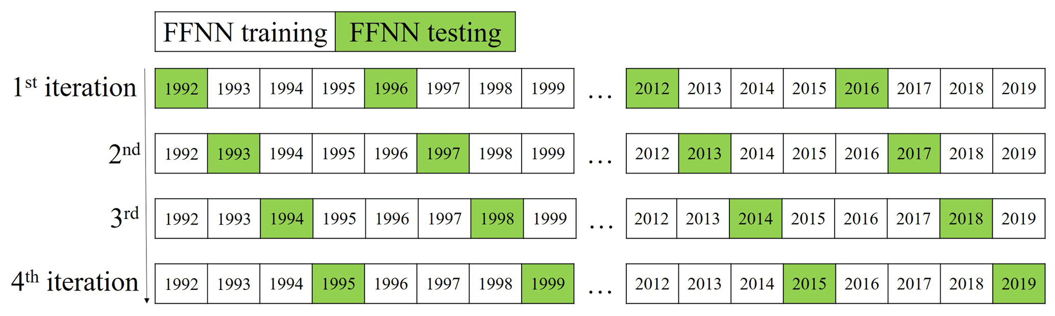
Figure 3 The K-fold validation procedure. (The K value was set as 4, so iterations were repeated 4 times until all samples were set as having tested samples once. In each iteration, samples in 7 years were set as testing samples (green cells) and in the rest 21 years were set as training samples (white cells) to increase independence.)

Table 3 Predictors in each biogeochemical province.

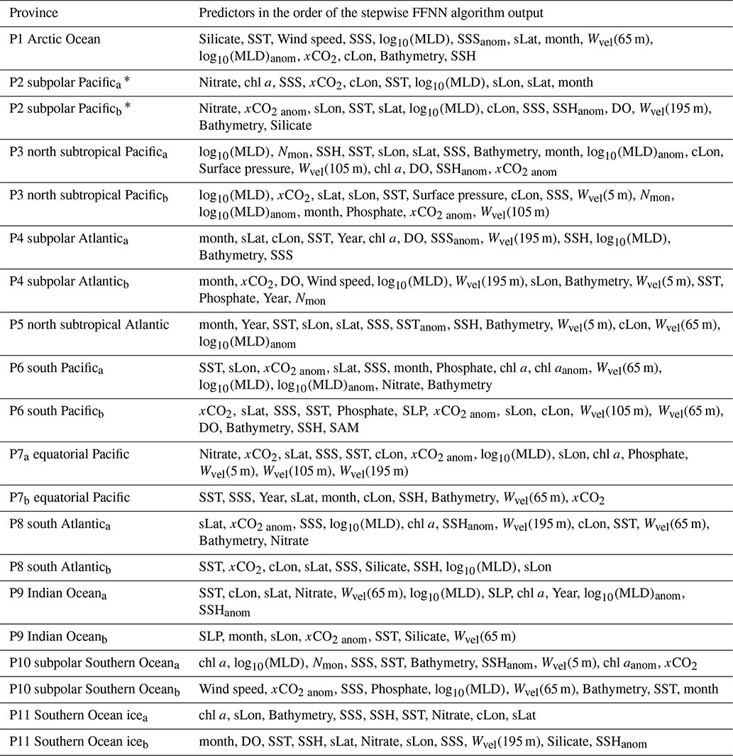
^∗: Due to insufficient coverage of chl a data in the polar areas and during the period before 2002, in provinces that chl a or chl a_anom were selected as predictors, the pCO₂ data were divided into two periods. The period with available chl a data was represented by the subscript ”a”, such as P2_a, including global grids from 2002 to 2019 except polar grids in winter. The period with unavailable chl a data was represented by the subscript ”b”, such as P2_b, including global grids from 1992 to 2001 and some polar grids in winter from 1992 to 2019.

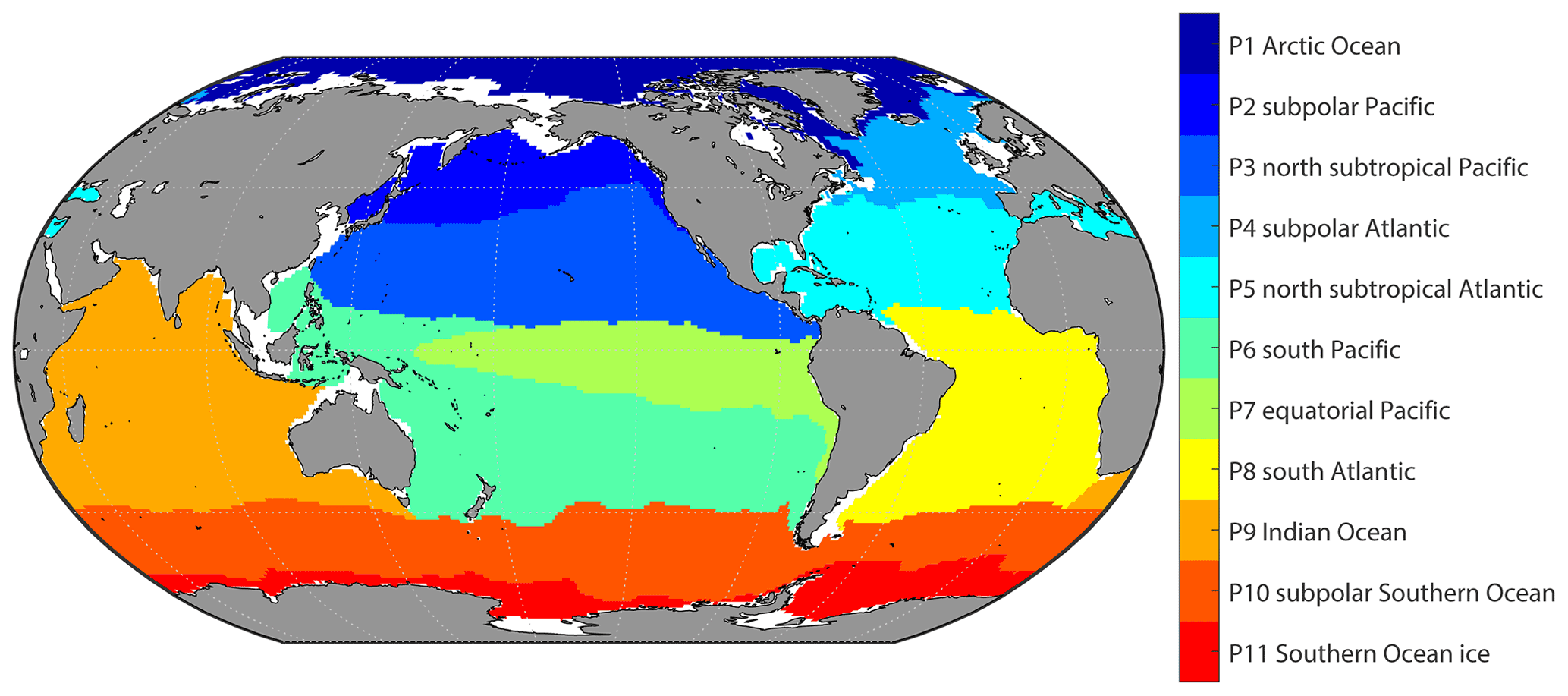
Figure 4 Map of biogeochemical provinces based on SOM.

3 Results and discussion

3.1 Biogeochemical provinces and corresponding predictors of pCO₂

11 biogeochemical provinces generated from the SOM method after the separated small “island” was removed and the province separated by lands was divided manually (Fig. 4). The results of the stepwise FFNN algorithm in each province are shown in Table 3. The predictors were listed in the order that the stepwise FFNN algorithm printed recommended predictors out. The predictor printed earlier was relatively more highly recommended and played an important role in predicting pCO₂ based on FFNN. Applying these predictors effectively decreased the predicting error between the FFNN outputs and pCO₂ values from validation samples. Thus it is reasonable to consider that these predictors were highly related to the drivers of pCO₂ and its variability. Predictors representing sampling positions were also listed as recommended predictors in some provinces, including latitude, longitude, and sampling time, suggesting that relatively steady spatial or temporal variability patterns of surface ocean pCO₂ existed in these biogeochemical provinces. For example, the predictor month was considered recommended in most provinces, especially P4 subpolar Atlantic and P5 north subtropical Atlantic, while pCO₂ in these areas regularly peaked and bottomed out in summer and winter (Takahashi et al., 2009; Landschützer et al., 2016, 2020). Similarly, the sine of latitude and the sine and cosine of longitude were listed as recommended predictors of pCO₂ in most provinces, suggesting a meridional or zonal uniformly varying spatial distribution pattern of pCO₂, which was not learned sufficiently by the FFNN model from existing measured predictors, and the predictors related to the spatial position were applied as supplementary.

As basic predictors highly related to the ocean environment, temperature and salinity were considered as parts of the most important predictors of surface ocean pCO₂ and were applied in the pCO₂ prediction in almost all previous related research based on various methods (Jo et al., 2012; Signorini et al., 2013; Landschützer et al., 2014; Marrec et al., 2015; Chen et al., 2016, 2017; S. Chen et al., 2019; Moussa et al., 2016; Laruelle et al., 2017; Zeng et al., 2017; Denvil-Sommer et al., 2019). The results of the stepwise FFNN algorithm also supported this. The temperature was listed as a recommended predictor in all biogeochemical provinces, suggesting that temperature was one of the most critical drivers of pCO₂ and its variability in these provinces. Similarly, results from the stepwise FFNN algorithm provide evidence for the importance of salinity in predicting pCO₂, which was also listed as a predictor in most provinces. The dry air mixing ratio of atmospheric CO₂ (xCO₂) and the monthly anomaly of xCO₂ were also recommended predictors in most biogeochemical provinces, suggesting that the exchange of CO₂ across the sea–air interface was also an important driver of surface ocean pCO₂. As a widely used predictor in pCO₂ prediction, the chlorophyll a concentration (chl a) played an essential role in fitting the influence of biological activities on pCO₂ in previous research (Landschützer et al., 2014; Zeng et al., 2017; Laruelle et al., 2017; Denvil-Sommer et al., 2019). Especially in the province P10 subpolar Southern Ocean and P11 Southern Ocean ice, chl a was listed as the most recommended predictor in the result of the stepwise FFNN algorithm, while in some other provinces (P1 Arctic Ocean and P5 north subtropical Atlantic), chl a was considered redundant in that no effective decrease of MAE between FFNN outputs and pCO₂ measurements appeared when the chl a data were used. Similar to the period where chl a was not available (represented by the subscript “b”), phosphate, nitrate, silicate, or dissolved oxygen were recommended instead. In the province P1 Arctic Ocean, silicate concentration and temperature were considered the most crucial predictors of pCO₂.

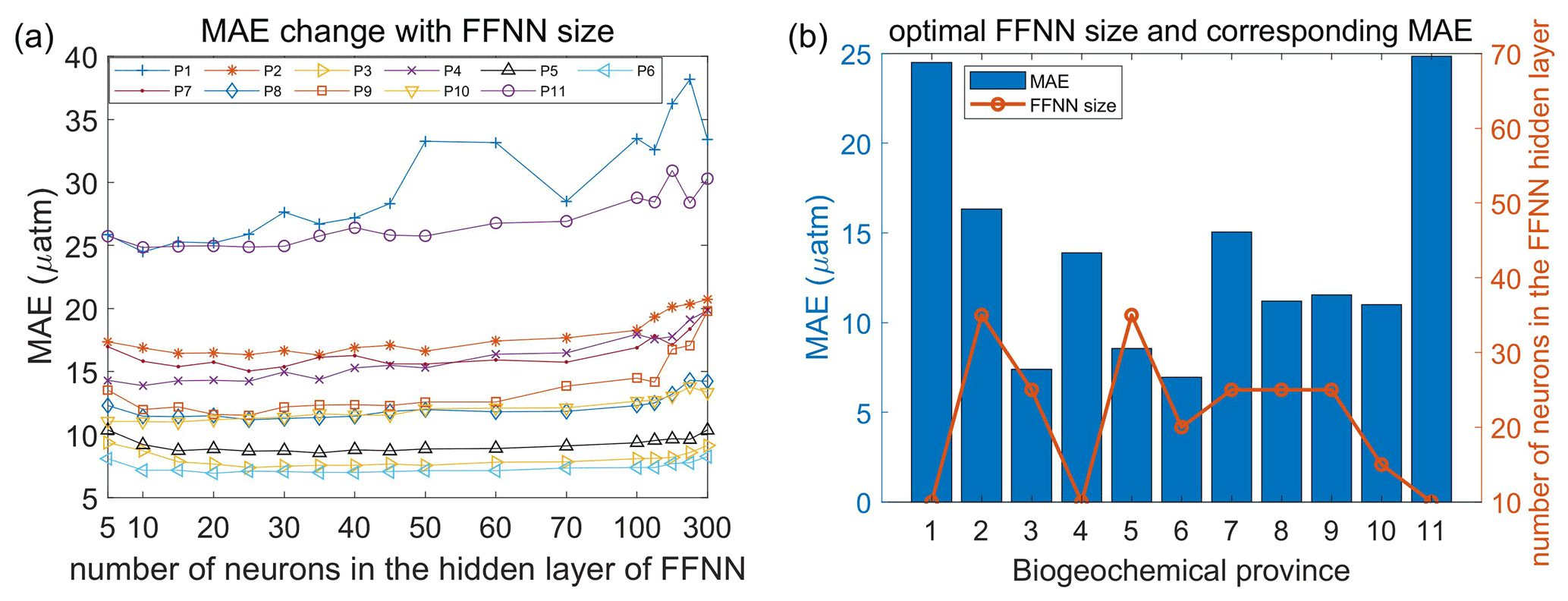
Figure 5 MAE of different FFNN size in each biogeochemical province. (a) MAE between predicted pCO₂ and SOCAT observations was calculated using the same samples and FFNN with a different number of neurons. (b) The optimal FFNN size refers to the number of neurons when MAE is lowest.

3.2 pCO₂ product

Based on the predictors given by the stepwise FFNN algorithm in each biogeochemical province, an FFNN size (representing the number of neurons in the hidden layer) improving validation was applied to decrease the prediction error further. The MAE values based on the same samples and FFNN model with a different number of neurons were calculated, then the number of neurons corresponding to the lowest MAE was applied (Fig. 5a). The MAE in most provinces tends to decrease first and then increase when the number of neurons in the hidden layer of the FFNN model increased from 5 to 300. Based on the variation of MAE with the number of neurons in the FFNN hidden layer, the optimal FFNN size in each province was considered as the number of neurons when the MAE was lowest. The result and corresponding MAE are shown in Fig. 5b. After applying optimal FFNN size in each province, the MAE and RMSE of global estimates between predicted pCO₂ and measurements from SOCAT v2020 further decreased to 11.32 and 17.99 µatm, respectively.

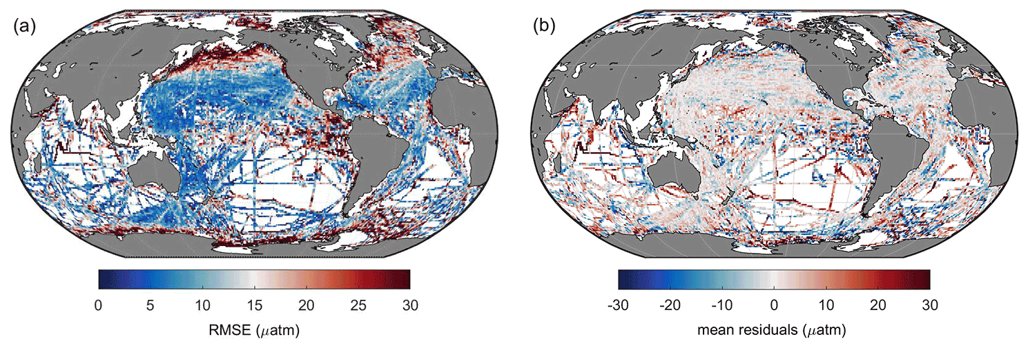
Figure 6 Global maps of (a) RMSE and (b) mean residuals between predicted pCO₂ and SOCAT observations.

Then the RMSE and mean residuals in each grid were calculated based on the K-fold cross validation method. In most grids, the RMSE was lower than 10 µatm, and the mean residuals were close to zero (Fig. 6). However, the prediction error in the north subpolar Pacific, the eastern equatorial Pacific, and the Southern Ocean near the Antarctic continent was significantly higher than in other areas. Also, the distribution of mean residuals suggested that surface ocean pCO₂ in the Indian Ocean tends to be overestimated by the FFNN models, while in other regions, the distribution of mean residuals was more discrete, and no obvious pattern was found.

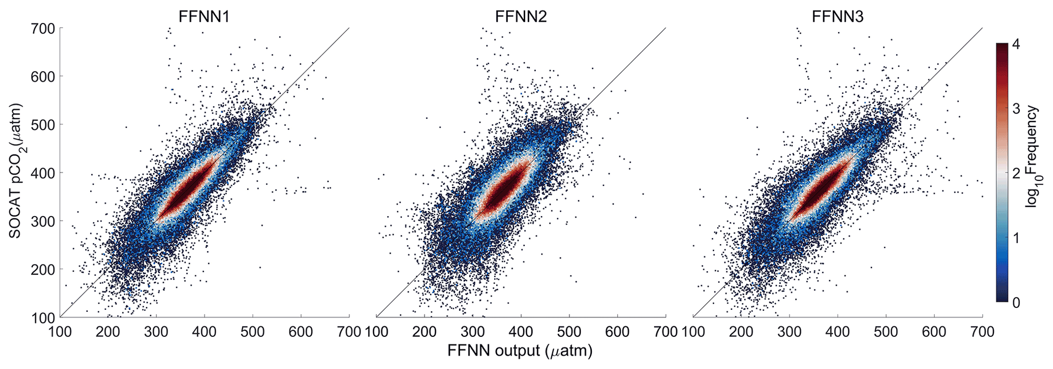
Figure 7 Comparison of FFNN-predicted pCO₂ with SOCAT pCO₂. FFNN1 was based on predictors selected by the stepwise FFNN algorithm. FFNN2 and FFNN3 were based on predictors from Landschützer et al. (2014) and Denvil-Sommer et al. (2019), respectively.

3.3 Validation of the stepwise FFNN algorithm based on SOCAT samples

Validation based on the K-fold cross validation method suggested that most FFNN outputs were quite close to the pCO₂ values from SOCAT v2020 samples (Fig. 7). Comparing the results based on a different combination of predictors, the results of FFNN1 (based on stepwise FFNN algorithm, this paper) and FFNN3 (based on 15 predictors from Denvil-Sommer et al. 2019) were more precise than those of FFNN2 (based on 10 predictors from Landschützer et al. 2014). The plots in the result of FFNN1 were most concentrated along the y=x line, suggesting extremely close FFNN outputs with the measured pCO₂ values from SOCAT, with the RMSE of 17.99 µatm in the global open oceans. The RMSE of FFNN1 was lower than that of FFNN2 (22.95 µatm) and FFNN3 (19.17 µatm).

Table 4 Performance of pCO₂ prediction based on different predictors.

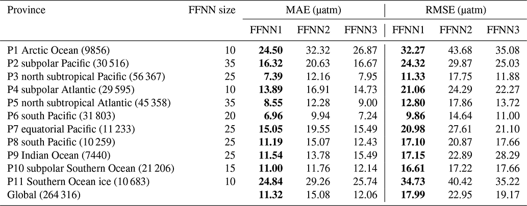
FFNN1 was based on predictors selected by the stepwise FFNN algorithm. FFNN2 and FFNN3 were based on predictors from Landschützer et al. (2014) and Denvil-Sommer et al. (2019), respectively. The lowest MAE and RMSE between different validation groups was shown in bold. The number in parentheses after the province name is the number of SOCAT monthly mean samples for that province.

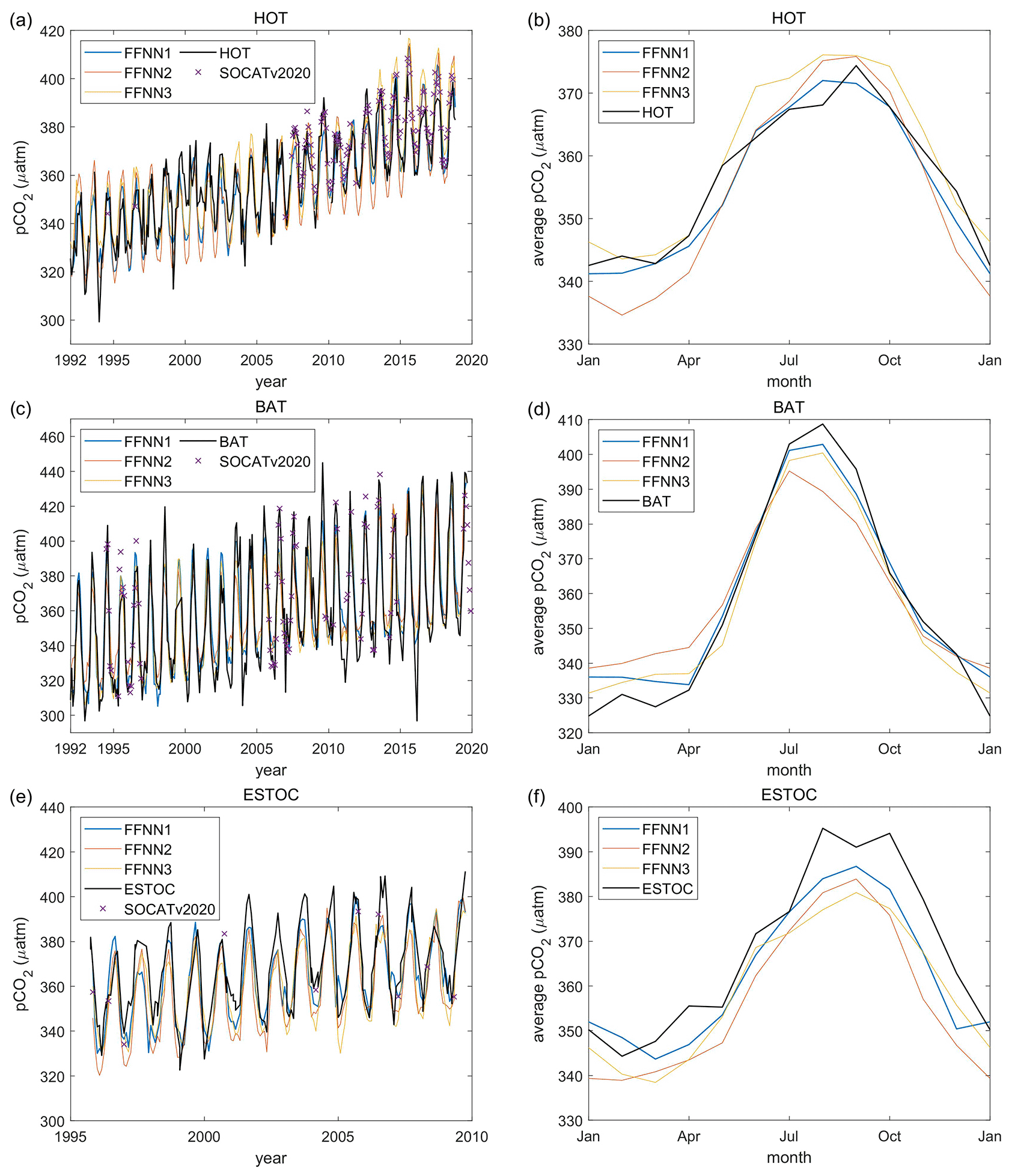
Figure 8 Validation based on independent observation from time series stations: (a, b) the Hawaii Ocean Time-series (HOT; Dore et al., 2009); (c, d) the Bermuda Atlantic Time-series Study (BATS; Bates, 2007); (e, f) the European Station for Time Series in the Ocean Canary Islands (ESTOC; González-Dávila and Santana-Casiano, 2012). FFNN1 was based on predictors selected by the stepwise FFNN algorithm. FFNN2 and FFNN3 were based on predictors from Landschützer et al., 2014 and Denvil-Sommer et al., 2019, respectively. SOCATv2020 represents the monthly mean pCO₂ of SOCAT observations in the corresponding grids of each time series station.

For specific comparison of accuracy in each province, the MAE of FFNN1 was lower in most provinces (Table 4), except for the relatively close results between the FFNN1 and FFNN3 in parts of the provinces. The MAE of FFNN1 in the province P9 Indian Ocean was significantly lower than that of the other validation groups, suggesting a better combination of predictors highly related to the drivers of surface ocean pCO₂ and its variability in the Indian Ocean. Compared with FFNN2 and FFNN3, the predictors of FFNN1 added surface pressure and W velocity of ocean currents and abandoned the monthly anomalies of other predictors in the province P9 Indian Ocean. The low relevance between pCO₂ and part of the monthly anomalies, such as SSS_anom and SST_anom, may be responsible for the significantly lower MAE of FFNN1. Adding redundant predictors may cause misleading information in the learning of the FFNN model on the contrary. The MAE and RMSE differences between FFNN1 and FFNN3 in some provinces were relatively small. The reason for the higher MAE and RMSE of FFNN2 may be applying latitudes and longitudes as predictors in both FFNN1 and FFNN3 but not in FFNN2. In the province P10 subpolar Southern Ocean, latitudes and longitudes were considered not good predictors by the stepwise FFNN algorithm, and the results of three validation groups were extremely close.

3.4 Validation based on independent observations

The FFNN outputs based on a different combination of predictors were compared with independent observations from HOT (Dore et al., 2009), BATS (Bates, 2007), and ESTOC (González-Dávila and Santana-Casiano, 2012; Fig. 8). Compared with the independent observations from the HOT station, the three validation groups all show close results, which were also similar in the seasonal and interannual variability of pCO₂. From 1992 to 2019, the RMSE between FFNN1 outputs and HOT observations was only 9.29 µatm, lower than the 10.85 µatm of FFNN2 and the 10.70 µatm of FFNN3. The monthly mean pCO₂ of FFNN2 during winter was lower than the HOT observations and pCO₂ values of other validation groups, while the FFNN1 and FFNN3 outputs were closer to the HOT observations. The MAE between predicted pCO₂ and HOT observations was also lower in the validation group FFNN1, which was only 7.17 µatm, compared to the 8.61 µatm of FFNN2 and the 8.44 µatm of FFNN3. Higher bias was generated in the winter bottom and summer peak, shown more obviously in the monthly average of pCO₂ (Fig. 8b). Compared with other validation groups, the result of FFNN1 was closer to the monthly average values of the HOT observations. The same conclusion can be obtained for the ESTOC and BATS station located in the province P5 north subtropical Atlantic. The RMSE between FFNN1 outputs and independent observations was 13.03 µatm for the BATS station and 11.35 µatm for the ESTOC station, lower than other validation groups. The RMSE between FFNN2 outputs and independent observations was 16.15 µatm for the BATS station and 14.51 µatm for the ESTOC station. For the group FFNN3, the RMSE was 13.09 µatm for the BATS station and 13.01 µatm for the ESTOC station. All results were extremely close to the independent observations, but the RMSE and MAE of FFNN1 were lower. Similar to the situation in the HOT station, FFNN1 was closest and FFNN3 second-closest. Based on the better performance of FFNN1, in which the predictors selected by the stepwise FFNN algorithm were used, we may conclude that the stepwise FFNN algorithm can effectively find a better combination of predictors to fit the driver of surface ocean pCO₂ and obtain a lower error.

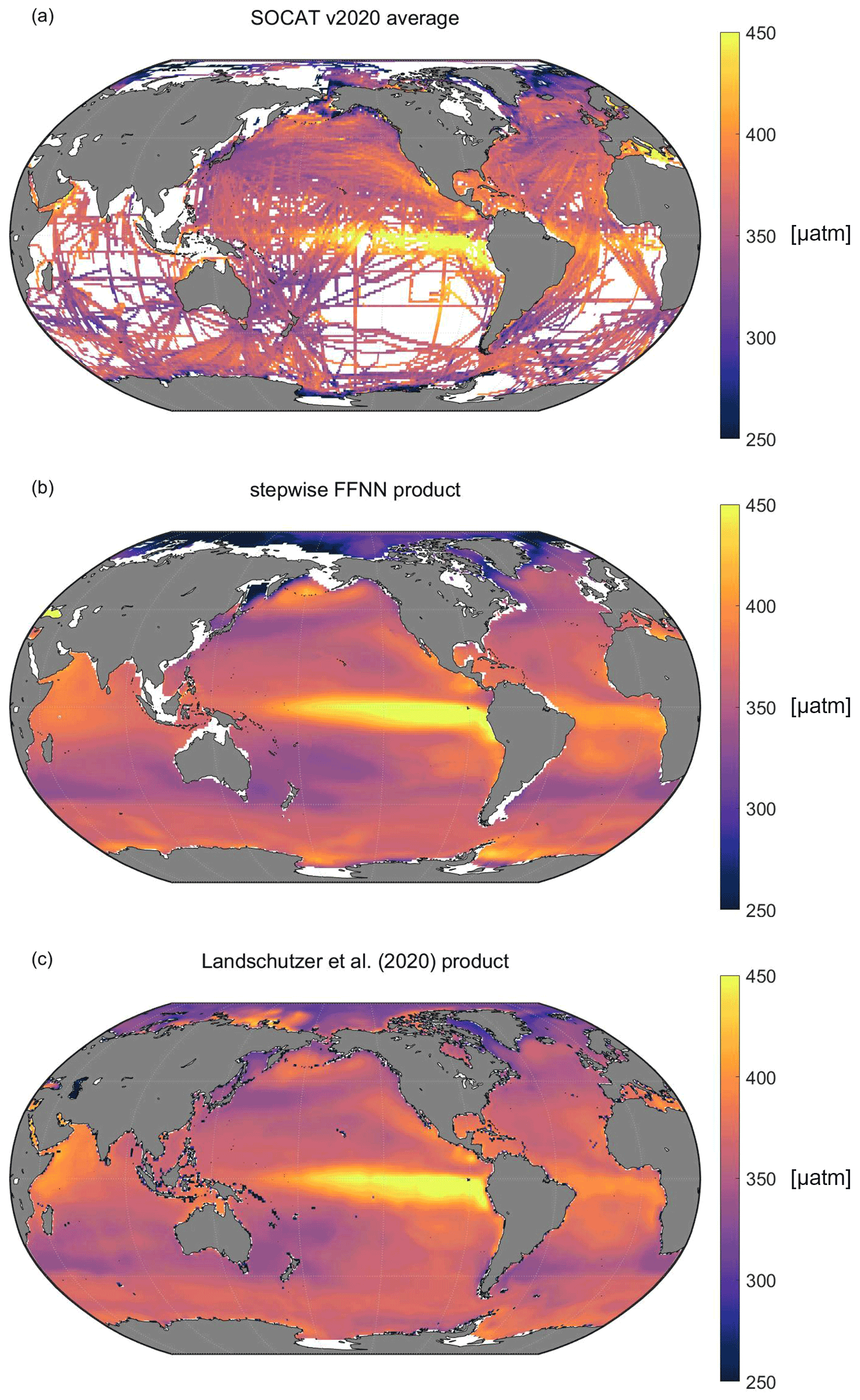
Figure 9 Comparison between the long-term average of (a) the SOCAT v2020 dataset, (b) the stepwise FFNN pCO₂ product, and (c) previous climatology product adapted from Landschützer et al. (2020).

3.5 Climatological spatial distribution

The climatological average distribution of pCO₂ suggested significant spatial variability (Fig. 9), consistent with the average distribution of SOCAT observations. In the Pacific Ocean, the high pCO₂ areas shown by the stepwise FFNN product (Fig. 9b), including the equatorial areas, east temperate areas, and north subpolar areas, were highly consistent with the SOCAT datasets (Fig. 9a). Similarly, the distribution of pCO₂ in the Atlantic Ocean was also close. However, the stepwise FFNN product suggested lower pCO₂ average values in the Arctic and higher values in the Southern Ocean near the Antarctic continent. Compared with the previous climatology product (Landschützer et al., 2020), the stepwise FFNN product has similar spatial patterns with high pCO₂ in the eastern equatorial Pacific and equatorial Atlantic: an inconsistent spatial distribution also existed in the Arctic and parts of the Southern Ocean near the Antarctic continent. The differences between the stepwise FFNN product and the previous climatology product may be caused by differences in methods or SOCAT dataset versions used. In comparison, lower average values of the SOCAT dataset in the Southern Ocean may be caused by the undersampling in winter. The global spatial distribution pattern of the stepwise FFNN pCO₂ product was basically well consistent with the previous climatology product and SOCAT dataset, suggesting that pCO₂ predicting based on regional specific predictors selected by the stepwise FFNN algorithm was better than that based on the globally same predictors.

4 Conclusions

A stepwise FFNN algorithm was constructed to decrease the predicting error in the surface ocean pCO₂ mapping by finding better combinations of pCO₂ predictors in each biogeochemical province defined by the SOM method, based on which a monthly 1^∘ × 1^∘ gridded global open-oceanic surface ocean pCO₂ product from January 1992 to August 2019 was constructed. Our work provided a statistical method for predictor selection for all research based on relationship fitting by machine learning methods. The validation based on the SOCAT dataset and independent observations shows that using regional-specific predictors selected by the stepwise FFNN algorithm retrieved a lower predicting error than globally similar predictors. This stepwise FFNN algorithm can also be used in pCO₂ mapping research for higher resolution and coastal regions, and in other data mapping research using SOM or other region dividing methods. The preparation work consisted only of collecting as many predictors as possible that might be related to the target data, and they need to be sufficiently available in time and space. However, high predicting error in particular regions, such as polar regions and the equatorial Pacific, still needs to be improved. Since the stepwise FFNN algorithm's result largely depends on how biogeochemical provinces are divided, improving the SOM step is still necessary. In addition, the FFNN can be replaced by any suitable type of neural network. A possible way to improve the performance of the stepwise FFNN algorithm is to modify the structure of the FFNN or to use networks with more sophisticated architecture and to use different learning algorithms. In future work, the stepwise FFNN algorithm with possible improvement will be attempted for the mapping of other products, such as total alkalinity and pH in order to provide sufficient data support for studies on ocean acidification and carbon cycling.