Assimilation of multiple datasets results in large differences in regional- to global-scale NEE and GPP budgets simulated by a terrestrial biosphere model

In spite of the importance of land ecosystems in offsetting carbon dioxide emissions released by anthropogenic activities into the atmosphere, the spatiotemporal dynamics of terrestrial carbon fluxes remain largely uncertain at regional to global scales. Over the past decade, data assimilation (DA) techniques have grown in importance for improving these fluxes simulated by terrestrial biosphere models (TBMs), by optimizing model parameter values while also pinpointing possible parameterization deficiencies. Although the joint assimilation of multiple data streams is expected to constrain a wider range of model processes, their actual benefits in terms of reduction in model uncertainty are still under-researched, also given the technical challenges. In this study, we investigated with a consistent DA framework and the ORCHIDEE-LMDz TBM–atmosphere model how the assimilation of different combinations of data streams may result in different regional to global carbon budgets. To do so, we performed comprehensive DA experiments where three datasets (in situ measurements of net carbon exchange and latent heat fluxes, spaceborne estimates of the normalized difference vegetation index, and atmospheric CO₂ concentration data measured at stations) were assimilated alone or simultaneously. We thus evaluated their complementarity and usefulness to constrain net and gross C land fluxes. We found that a major challenge in improving the spatial distribution of the land C sinks and sources with atmospheric CO₂ data relates to the correction of the soil carbon imbalance.

1 Introduction

The dramatic growth of atmospheric CO₂ concentrations recorded in the last half-century has increased awareness on the impact of human activities on climate. Taking up about one-third of the carbon dioxide from the atmosphere, the terrestrial biosphere plays a key role in regulating CO₂ emissions released by anthropogenic activities (fossil fuel emissions, land use and land cover change) (Friedlingstein et al., 2020). Quantifying variations in the distribution and intensity of carbon (C) sources and sinks from year to year remains a challenge given the complexity of the processes involved and what we can learn from observations. By formalizing current knowledge of the main processes governing the functioning of vegetation into numerical representations, terrestrial biosphere models (TBMs) have grown in importance for studying the spatiotemporal dynamics of net and gross land surface C fluxes from the local to the global scale. However, the large spread in simulated regional- to global-scale C fluxes for the last few decade (Friedlingstein et al., 2020) as well as for future projections (Arora et al., 2020) highlights the remaining uncertainties in our understanding and prediction of the fate and role of the biosphere under climate change and anthropogenic pressure.

Over the past decade, the parameter uncertainty in TBMs has increasingly been reduced thanks to statistical data assimilation (DA; also referred to as model–data fusion) frameworks, benefiting from the experience gained in other fields of Earth and environmental sciences (geophysics, weather forecasting, hydrology, oceanography, etc.). DA techniques enable optimization of the model parameters using relevant target observations while taking into account both observational and modeling uncertainties. DA does not only enable improvement of the model parameters, but can also help pinpoint model deficiencies (Luo et al., 2012). The importance of DA as a key component of terrestrial biosphere carbon cycle modeling is reflected by the diversity of DA systems in the global TBM communities. Since the first global-scale Carbon Cycle Data Assimilation System (CCDAS) (Kaminski et al., 2002; Rayner et al., 2005) developed for the Biosphere Energy Transfer Hydrology (BETHY) model, other modeling groups have developed their own global-scale carbon cycle DA systems, in particular for ORCHIDEE (ORganizing Carbon and Hydrology In Dynamic EcosystEms model) (Santaren et al., 2007; Peylin et al., 2016), JULES (Joint UK Land Environment Simulator) (Raoult et al., 2016), JSBACH (Schürmann et al., 2016), or CLM (Community Land Model) (Fox et al., 2018), and in parallel to the development of community assimilation tools such as DART (Anderson et al., 2009) or PECAn (Dietze et al., 2013).

Within a variational DA framework, ground-based measurements of eddy-covariance fluxes at a local scale (Wang et al., 2001; Knorr and Kattge, 2005; Sacks et al., 2007; Williams et al., 2009; Groenendijk et al., 2011; Kuppel et al., 2012) have been widely used to constrain net and gross CO₂ fluxes and latent heat flux. Moreover, remote sensing proxies of vegetation activities, such as raw reflectance data (Quaife et al., 2008), vegetation indices (Migliavacca et al., 2009; MacBean et al., 2015), or FAPAR – fraction of absorbed photosynthetically active radiation (Stöckli et al., 2008; Zobitz et al., 2014; Forkel et al., 2014; Bacour et al., 2015), have also been used to constrain the model parameters at various spatial scales. Finally, atmospheric CO₂ mole fraction measurements have been assimilated to provide valuable information on large-scale net ecosystem exchange (NEE) (Rayner et al., 2005; Koffi et al., 2012).

In the early days of DA studies, most focused on the assimilation of a single data stream (e.g., targeting only NEE). Then, assimilations with multiple C-cycle-related datasets were soon considered (Moore et al., 2008; Richardson et al., 2010; Ricciuto et al., 2011; Keenan et al., 2013; Thum et al., 2017; Knorr et al., 2010; Kaminski et al., 2012; Kato et al., 2013; Bacour et al., 2015; Peylin et al., 2016). The underlying motivation behind assimilating multiple data streams is that using a greater number and diversity of observations should provide stronger constraints on model parameters, including a wider range of processes, hence resulting in a greater reduction in model uncertainty. However, many previous studies that assimilated multiple datasets hardly considered potential incompatibilities between the model and the observations (although see Bacour et al., 2015; Thum et al., 2017), which may result in a deterioration of model agreement with other observations not included in the assimilation. In addition, only a few have quantified the actual benefit of assimilating multiple datasets compared to the single data stream assimilations, in particular in the context of global-scale C cycle DA experiments.

The assimilation of multiple data streams can be done either sequentially, in which one observation type is assimilated at a time, or simultaneously (joint assimilation approach or “batch” strategy as defined in Raupach et al., 2005), where the model is calibrated with all data included in the same optimization (e.g., Richardson et al., 2010; Kaminski et al., 2012; Schürmann et al., 2016). Although with model parameters and observations described by probability distributions, simultaneous and sequential assimilations could theoretically lead to the same result (Tarantola et al., 2005), this is not the case in practice for complex problems. Incomplete or incorrect description of the error statistics may result in large differences between simultaneous and stepwise approaches (see Kaminski et al., 2012; MacBean et al., 2016). In addition, model nonlinearities also tend to exacerbate these potential differences. Simultaneous assimilation is considered to be more optimal in the context of optimizing TBM parameters as it maximizes the consistency of the model with the whole of the datasets considered (Richardson et al., 2010; Kaminski et al., 2012) and avoids incorrect/incomplete propagation of the error statistics from one step to the other (Peylin et al., 2016). The use of a gradient descent approach for the optimization, with the risk that it gets trapped in local minima, also increases the chances that stepwise and simultaneous approaches diverge. However, sequential approaches remain appealing for modelers: they require less initial technical investment and enable easier assessment of the impact of each data stream assimilated successively onto the optimized variables. Both approaches however face similar challenges, like defining the model–data uncertainty (see, e.g., Richardson et al., 2010; Keenan et al., 2013; Kaminski et al., 2012; Bacour et al., 2015; Thum et al., 2017; Peylin et al., 2016) and hence the weight that each dataset has on the optimization outcome (although specific weighting approaches may be envisioned, as in Wutzler and Carvalhais et al., 2014, or Oberpriller et al., 2021). Another major challenge, as highlighted by MacBean et al. (2016) or Oberpriller et al. (2021), concerns inconsistencies between observations and model outputs, which are usually not accounted for in common bias-blind (Dee, 2005) Bayesian DA systems relying on the hypothesis of Gaussian errors. Indeed, most studies do not attempt to identify systematic errors in the observations and/or in the model and to correct for them. The likely impact of model–data biases on the parameter optimization is then a degraded model performance as well as an illusory decrease in the estimated model uncertainty (Wutzler and Carvalhais, 2014; MacBean et al., 2016; Bacour et al., 2019a).

The present study aims to go a step forward in the assessment of how assimilating multiple C-cycle-related data streams impacts and changes the constraint on net and gross CO₂ flux simulations at the global scale. To do so, we further advance from the sequential assimilation of Peylin et al. (2016) (referred to as the “stepwise” approach hereafter) by implementing a simultaneous assimilation framework with the same data streams: net carbon fluxes (net ecosystem exchange – NEE) and latent heat fluxes (LE) measured at eddy-covariance sites across different ecosystems, satellite-derived normalized difference vegetation index (NDVI) at coarse resolution for a set of pixels spanning the main deciduous vegetation types, and monthly atmospheric CO₂ concentration data measured at surface stations worldwide. The study relies on the variational DA framework designed for the ORCHIDEE global vegetation model (Krinner et al., 2005), here associated with a simplified version of the LMDz atmospheric transport model (Atmospheric General Circulation Model of the Laboratoire de Météorologie Dynamique; Hourdin et al., 2006) based on precalculated transport fields for assimilating atmospheric CO₂ concentration data. ORCHIDEE and LMDz are the terrestrial and atmospheric components of the Institut Pierre Simon Laplace (IPSL) Earth System Model (Dufresne et al., 2013).

By conducting different assimilation experiments in which each data stream is assimilated alone or in combination (for all combinations of datasets), the research questions that we address in this study are as follows:

1. What impact does the combination of different data streams assimilated have on the reduction in model–data misfit, and to which extent are the model predictions improved (or degraded) with respect to the other data streams that were not assimilated?

2. How does the combination of different data streams impact the optimized parameter values and uncertainties and the predicted spatial distribution of the net and gross carbon fluxes at regional and global scales? How do the derived carbon budgets compare with independent process-based model and atmospheric inversion estimates from the Global Carbon Project's 2020 Global Carbon Budget (Friedlingstein et al., 2020)?

3. How does a model–data bias related to incorrect initialization of soil carbon pools (i.e., their disequilibrium with respect to steady state) impact the overall optimization performances within a Bayesian assimilation framework relying on the hypothesis of Gaussian errors?

In addition, our analysis of the useful informational content provided by different data streams on C fluxes is supported by methodological aspects aiming to do the following:

1. Improve the realism of the prior error statistics on parameters by making them consistent with the prior model–data mismatch.

2. Quantify the observation influence of each of the three data streams on the joint assimilation in which all three datasets were included in the optimization.

Throughout the presentation of the results, we discuss implications of each assimilation experiment for our ability to accurately constrain gross and net CO₂ fluxes. In the final section we propose some perspectives for other modeling groups wishing to implement global-scale parameter DA systems to constrain regional- to global-scale C budgets.

2 Materials and methods

2.1 Models

2.1.1 ORCHIDEE

Model description

ORCHIDEE is a spatially explicit process-based global TBM (Krinner et al., 2005) that calculates the fluxes of carbon dioxide, water and heat, between the biosphere and the atmosphere, as well as the soil water budget. The temporal resolution is half an hour except for the slow components of the terrestrial carbon cycle (including carbon allocation in plant reservoirs, soil carbon dynamics and litter decomposition) which are calculated on a daily basis. The version of ORCHIDEE in this study corresponds to that used in the IPSL Earth System Model for its contribution to the Climate Model Intercomparison Project 5 (CMIP5) established by the World Climate Research Program. Vegetation is represented by 13 plant functional types (PFTs) that include bare soil. The processes use the same governing equations for all PFTs, except for the seasonal leaf dynamics (phenology), which follows Botta et al. (2000) (see MacBean et al., 2015, for a full description). The observation operator for NDVI is determined (i) by assuming a linear relationship between NDVI and FAPAR (Myneni et al., 1994) and (ii) by calculating FAPAR from the simulated leaf area index (LAI) based on the classical Beer–Lambert law for the extinction of the direct illumination within the canopy (Bacour et al., 2015; MacBean et al., 2015). In addition, we consider normalized data in our assimilation scheme. The soil organic carbon is simulated by a CENTURY-type model (Parton et al., 1987) and is partitioned in three pools (slow, passive and active) with different residence times.

Model setup

The setup of the simulations performed with ORCHIDEE depends on the data assimilated. The model is run at site scale for the assimilation of eddy-covariance measurements, at a spatial resolution of 0.72^∘ for the assimilation of the satellite NDVI data and at the resolution of the atmospheric transport model LMDz ($\mathrm{3.75}{}^{\circ }\times \mathrm{2.5}{}^{\circ }$) for the assimilation of atmospheric CO₂ measurements. The Olson land cover classification at 5 km is used to derive the PFT fractions at each spatial resolution but for the flux tower simulations where the proportion of each PFT is set based on expert knowledge. For satellite pixels and global simulations, ORCHIDEE is forced using the 3-hourly ERA-Interim gridded meteorological forcing fields (Dee et al., 2011) (aggregated at $\mathrm{3.75}{}^{\circ }\times \mathrm{2.5}{}^{\circ }$ when assimilating atmospheric CO₂ concentrations). For the flux tower simulations, the model is forced by local measurements of the meteorological variables at a half-hourly time step.

For each spatial resolution, a prior spin-up simulation was performed by recycling available forcing data. The objective was to bring the different soil carbon reservoirs to “realistic” values, though the spin-up runs result in neutral net carbon flux by construction. Each spin-up simulation was then followed by a transient simulation (starting from the first year of measurement for each data stream), accounting for the secular increase of atmospheric CO₂ concentrations; for the global simulations, only a short transient simulation from 1990 to 1999 was performed.

2.1.2 LMDz

Model description

The study relies on version 3 of LMDz (Hourdin et al., 2006) as implemented for the IPSL contribution to CMIP4. In order to save computational time, we used LMDz in the form of a precomputed Jacobian matrix at a set of CO₂ measurement stations (Sect. 2.2.3) (see details in Peylin et al., 2016).

Model setup

To simulate atmospheric CO₂ concentrations that can be compared to observations, the transport model has to be forced not only by terrestrial biospheric fluxes (calculated by ORCHIDEE), but also by other natural (e.g., ocean) and anthropogenic CO₂ fluxes.  We imposed a net emission due to land use change (i.e., deforestation) of 1.1 GtC yr⁻¹, although we also accounted for a larger flux from biomass burning but which was compensated for partly by forest regrowth (see Peylin et al., 2016, for more details). The global maps of biomass burning emissions were taken from the Global Fire Emission Database version 3 dataset (Van der Werf et al., 2006; Randersen et al., 2013) over the period 1997–2010 at a monthly time step and gridded at $\mathrm{0.5}{}^{\circ }\times \mathrm{0.5}{}^{\circ }$ resolution. The global fossil fuel CO₂ emission products used here were developed by the University of Stuttgart/IER based on EDGAR v4.2 and were provided at a $\mathrm{0.1}{}^{\circ }\times \mathrm{0.1}{}^{\circ }$ spatial resolution and at a monthly timescale. The ocean flux component was obtained from a data-driven statistical model based on artificial neural networks that estimated the spatial and temporal variations of the air–sea CO₂ fluxes (Peylin et al., 2016).

Figure 1 Location of the flux tower sites (circles), satellite pixels (triangles) and atmospheric CO₂ stations (black stars) used in this study.

2.2 Assimilated data

2.2.1 In situ flux measurements (F)

The NEE and LE measurements come from the FLUXNET global network. We used harmonized, quality-checked and gap-filled data (Level 4) at 68 sites from the La Thuile global synthesis dataset (Papale, 2006). The site locations are presented in Fig. 1. These ecosystem measurements cover very different time spans, ranging from 1 single year at some sites up to 9 years. They constrain seven PFTs among the 12 natural vegetation types represented in ORCHIDEE: tropical evergreen broadleaf forest – TrEBF (3 sites corresponding to 6 site years), temperate evergreen needleleaf forest – TeENF (16 sites, 45 site years), temperate evergreen broadleaf forest – TeEBF (2 sites, 4 site years), temperate deciduous broadleaf forest – TeDBF (11 sites, 37 site years), boreal evergreen needleleaf forest – BoENF (12 sites, 44 site years), boreal deciduous broadleaf forest – BoDBF (3 sites, 6 site years), and C₃ grassland – C3GRA (21 sites, 56 site years). We assimilated daily-mean values of NEE and LE observations but only when at least 80 % of the 48 potential half-hourly data in a day are available.

2.2.2 Satellite products (VI)

The NDVI products considered here are derived from MODIS collection 5 surface reflectance data acquired in the red and near-infrared channels and corrected from the directional effects (Vermote et al., 2008). Data already assimilated into ORCHIDEE and described in MacBean et al. (2015) are considered here: they are provided at daily/0.72^∘ resolutions and span the 2000–2010 period. Five among the six deciduous, non-agricultural PFTs of ORCHIDEE were optimized in this study: TrDBF – tropical broadleaved rainy green forest, TeDBF, BoDBF, BoDNF – boreal needleleaf summergreen forest and C3GRA. C₄ grasses and evergreen PFTs were not considered. For each PFT, 15 0.72^∘ pixels were selected for assimilation depending on their thematic homogeneity with respect to the considered PFT (fractional coverage above 60 %) and consistency between the observed NDVI time series and the prior ORCHIDEE. The location of these satellite pixels is shown in Fig. 1.

2.2.3 Atmospheric CO₂ measurements (CO2)

The surface atmospheric CO₂ concentration data come from the NOAA Earth System Laboratory (ESRL) GLOBALVIEW-CO2 collaborative product (GLOBALVIEW-CO2, 2013). The data include in situ measurements, made by automated quasi-continuous analyzers, and air samples collected in flasks and later analyzed at central facilities. In this study, we used monthly-mean values of these measurements (Peylin et al., 2016). A period of 10 years of observations over the 2000–2009 period was used from a total of 53 stations located around the world (Fig. 1).

2.3 Assimilation methodology

2.3.1 Data assimilation framework

The data assimilation system associated with the ORCHIDEE model (ORCHIDAS) has been described in previous studies regarding the assimilation of these data streams alone (Kuppel et al., 2012; Santaren et al., 2014; MacBean et al., 2015; Bastrikov et al., 2018) or their combinations (Bacour et al., 2015; Peylin et al., 2016). The assimilation system relies on a variational Bayesian framework that optimizes ORCHIDEE parameters gathered in a vector x, by finding the minimum of a global misfit function J(x) iteratively. J(x) is a linear combination of the misfit functions associated with each data stream. It is assumed that the errors of observations and on the model parameters are Gaussian and that the data stream errors are independent from each other:

$$\begin{array}{}\text{(1)}& \begin{array}{rl}& J\left(\mathit{x}\right)={\displaystyle \frac{\mathrm{1}}{\mathrm{2}}}\left[{\left(H_{\text{LMDz}}\circ H_{\text{ORCH}}\left(\mathit{x}\right)-{\mathit{y}}^{\mathrm{CO}\mathrm{2}}\right)}^T\right.\\ & \cdot {\mathbf{R}}_{{\mathrm{CO}}_{\mathrm{2}}}^{-\mathrm{1}}\cdot \left(H_{\text{LMDz}}\circ H_{\text{ORCH}}\left(\mathit{x}\right)-{\mathit{y}}^{\mathrm{CO}\mathrm{2}}\right)\\ & +{\left(H_{\text{ORCH}}\left(\mathit{x}\right)-{\mathit{y}}^{\text{F}}\right)}^T\\ & \cdot {\mathbf{R}}_{\text{F}}^{-\mathrm{1}}\left(H_{\text{ORCH}}\left(\mathit{x}\right)-{\mathit{y}}^{\text{F}}\right)+{\left(H_{\text{ORCH}}\left(\mathit{x}-{\mathit{y}}^{\text{VI}}\right)\right)}^T\\ & \cdot {\mathbf{R}}_{\text{VI}}^{-\mathrm{1}}\left(H_{\text{ORCH}}\left(\mathit{x}\right)-{\mathit{y}}^{\text{VI}}\right)+{\left(\mathit{x}-{\mathit{x}}^{\text{b}}\right)}^T{\mathbf{B}}^{-\mathrm{1}}\\ & \left.\cdot \left(\mathit{x}-{\mathit{x}}^{\text{b}}\right)\right],\end{array}\end{array}$$

where y^o denotes the observation vectors (with o = F (flux), VI (satellite NDVI) or CO₂ (CO₂ concentration); H_ORCH and H_LMDz are the observational operators of the ORCHIDEE and LMDz models, respectively. R_o is the error covariance matrix characterizing the observation errors with respect to the model (therefore including the uncertainty in the model structure) associated with the data stream o. The dimensionless control vector z quantifies the distance between the values of the optimized parameters and the corresponding prior information ${\mathit{x}}^{\text{b}}:\mathit{z}={\mathbf{B}}^{-\mathrm{1}/\mathrm{2}}\cdot (\mathit{x}-{\mathit{x}}^{\text{b}}$), where B is the associated a priori error covariance matrix.

We use the gradient-based L-BFGS-B algorithm (Byrd et al., 1995; Zhu et al., 1997) to minimize J(x) iteratively. It accounts for bounds in the parameter variations. The algorithm requires the gradient of the misfit function as an input in order to explore the parameter space:

$$\begin{array}{}\text{(2)}& \begin{array}{rl}& {\mathrm{\nabla }}_{x}J\left(\mathit{x}\right)={\mathbf{H}}_{{\mathrm{ORCH}}^{{\mathrm{CO}}_{\mathrm{2}}}}^T\cdot {\mathbf{H}}_{\mathrm{LMDz}}^T\\ & \cdot {\mathbf{R}}_{{\mathrm{CO}}_{\mathrm{2}}}^{-\mathrm{1}}\left(H_{\text{LMDz}}\circ H_{\text{ORCH}}\left(\mathit{x}\right)-{\mathit{y}}^{\mathrm{CO}\mathrm{2}}\right)\\ & +{\mathbf{H}}_{{\mathrm{ORCH}}^{\text{F}}}^{\text{T}}\cdot {\mathbf{R}}_{\text{F}}^{-\mathrm{1}}\left(H_{\text{ORCH}}\left(\mathit{x}\right)-{\mathit{y}}^{\text{F}}\right)\\ & +{\mathbf{H}}_{{\mathrm{ORCH}}^{\mathrm{VI}}}^T\cdot {\mathbf{R}}_{\mathrm{VI}}^{-\mathrm{1}}\left(H_{\text{ORCH}}\left(\mathit{x}\right)-{\mathit{y}}^{\mathrm{VI}}\right)\\ & +{\mathbf{B}}^{-\mathrm{1}}(\mathit{x}-{\mathit{x}}^{\text{b}}).\end{array}\end{array}$$

The calculation of ∇_xJ(x) uses the Jacobian matrix of ORCHIDEE associated with each data stream, ${\mathbf{H}}_{{\text{ORCH}}^{\text{o}}}$ (assuming local linearity of the model), and that of LMDz. For most of the ORCHIDEE parameters, ${\mathbf{H}}_{{\text{ORCH}}^{\text{o}}}$ (or H^o hereafter) is calculated thanks to the tangent linear model of ORCHIDEE obtained by automatic differentiation using the TAF (Transformation of Algorithms in Fortran) tool (Giering et al., 2005); however, for a few parameters involved in threshold conditions of the model processes, especially related to phenology, we use a finite difference method.

After optimization, the posterior error covariance matrix A (for “analysis”) of the optimized parameters can be calculated as a function of the Jacobian matrix associated with the gradients of the model outputs with respect to the parameters at the solution for each data stream:

$$\begin{array}{}\text{(3)}& \mathbf{A}={\left[\sum {\mathbf{H}}^{{\text{o}}^T}\cdot {\mathbf{R}}_{\text{o}}^{-\mathrm{1}}\cdot {\mathbf{H}}^{\text{o}}+{\mathbf{B}}^{-\mathrm{1}}\right]}^{-\mathrm{1}}.\end{array}$$

It is computed under the hypothesis of model linearity in the vicinity of the solution. The square root of the diagonal elements of B or A correspond to the standard deviation σ on model parameters.

Table 1 List of the ORCHIDEE parameters to be optimized and data streams that constrain them (F for in situ flux measurements, VI for normalized satellite NDVI data and CO₂ for atmospheric CO₂ concentration data).

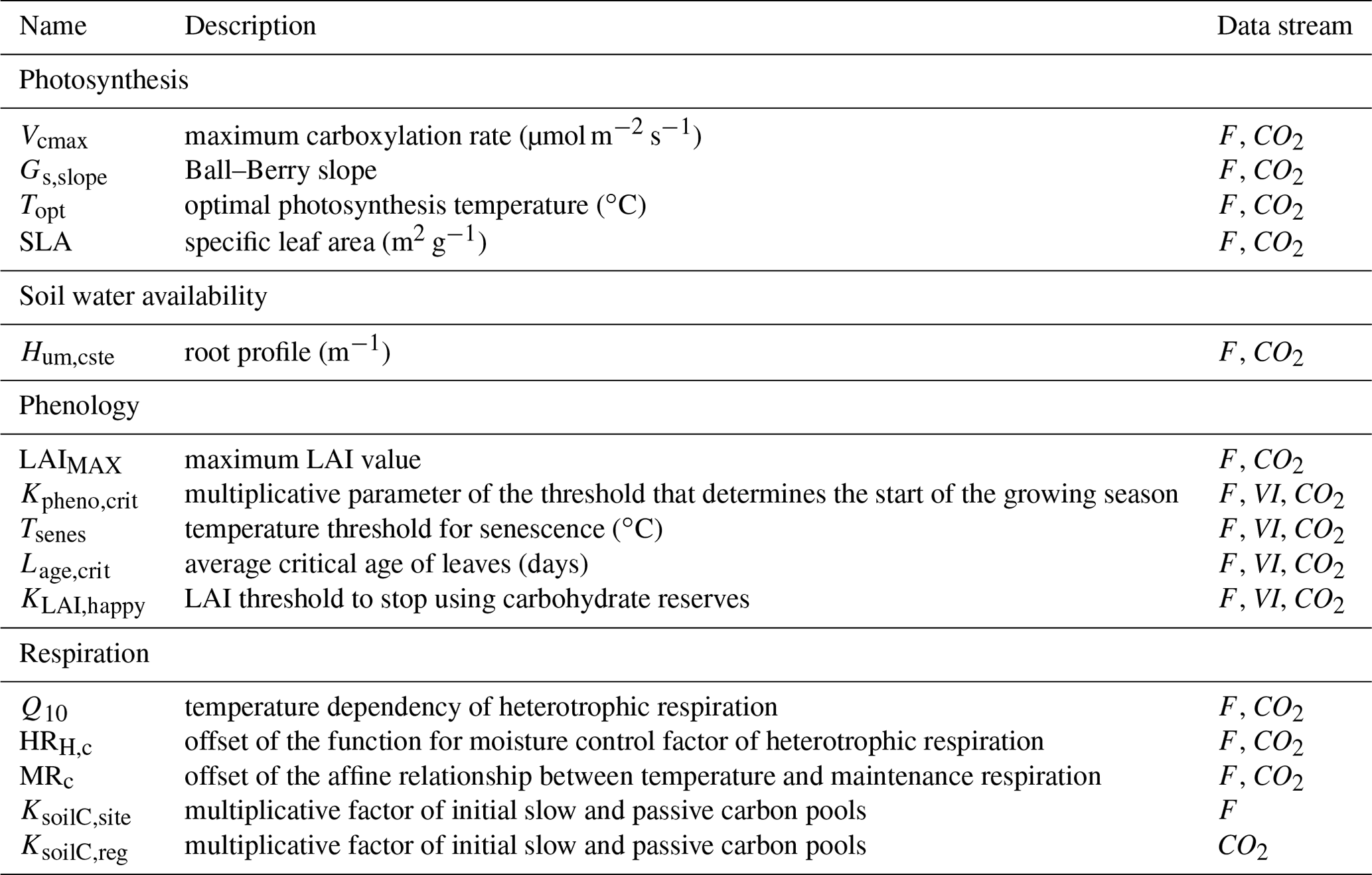
2.3.2 Parameters to be optimized

We chose to optimize a limited set of carbon-cycle-related parameters of ORCHIDEE as a result of preliminary sensitivity analyses and past DA studies. A short definition of these parameters that mostly control photosynthesis, phenology and respiration is provided in Table 1, while their associated prior values, bounds and uncertainty are documented in Table S3. More comprehensive descriptions of their role in the model processes are provided in Kuppel et al. (2012) and MacBean et al. (2015). The size of soil carbon pools drives the magnitude of the net carbon fluxes exchanged with the atmosphere to a large extent; soil carbon is closely related to soil texture and climatic (temperature and moisture) and disturbance history (including land use and fires), as well as ecosystem and edaphic properties (Schimel et al., 1994; Todd-Brown et al., 2013). Given that we do not have access to that information, neither at the site scale (for assimilation of NEE measurements) nor at the global scale (for assimilation of atmospheric CO₂ concentrations), we use a steady-state assumption where ORCHIDEE has been brought to near equilibrium with a long spin-up of the soil carbon pools. To correct for this bias, the initial state of the soil carbon reservoirs is optimized using a multiplicative parameter of both the slow and passive pools as in Peylin et al. (2016). The use of these correction factors is a handy way to correct any issues related to the use of our soil organic C model and the soil carbon disequilibrium. Two multiplicative parameters are used depending on the type of data considered (and their associated spatial scale): for in situ flux measurements, we considered site-specific parameters K_soilC,site; for atmospheric CO₂ concentration data, instead of resolving the initial conditions for all LMDz grid cells we scaled the carbon pools for 30 large-scale regions K_soilC,reg. Note that having correct soil carbon pools is less important when assimilating satellite NDVI data because these are more closely related to carbon uptake rather than net carbon flux. In total, up to 182 parameters are optimized depending on the data streams considered.

The prior values x^b of the parameters are set to the standard values of ORCHIDEE (Table S3). Not all parameters are constrained by all three data streams. In particular, satellite FAPAR/NDVI products inform the timing of phenology of plant vegetation (start and end of the growing season) rather than photosynthesis or respiration with our DA system (Bacour et al., 2015; MacBean et al., 2015). The dependency of each parameter with respect to the assimilated data streams is indicated in Table 1.

Table 2 Characteristics of the various assimilation experiments (flux data – F, satellite NDVI vegetation index – VI and atmospheric CO₂ concentration – CO2).

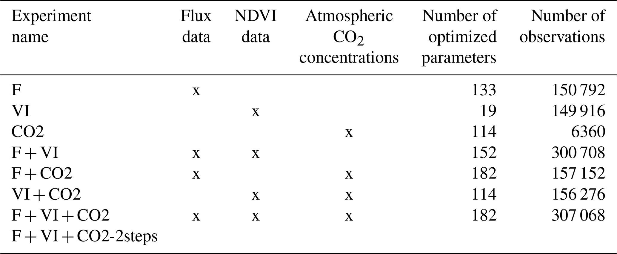
2.3.3 Data assimilation experiments

Different data assimilation experiments were tested in order to understand the respective constraint brought by each data stream and evaluate their compatibility with each other and with the model. First, each data stream was assimilated separately, and then its combinations with the other two were considered. Second, the three data streams were assimilated all together. The various experiments are described in Table 2, with the number of data points assimilated and the number of parameters optimized. Indeed, the number of optimized parameters differs with the type of data assimilated as described in Sect. 2.3.2 and in Table 1. The assimilations have a high computational cost, with an average value for joint assimilations using all three data streams of about 50 000 h central processing unit time on AMD Rome compute nodes, at 2.6 GHz with 256 GB memory per node.

Two assimilation experiments combining the three data streams were tested: one experiment (F + VI + CO2) with all parameters optimized in a single step; and an additional experiment following a two-step optimization (F + VI + CO2-2steps), as described hereafter. In the first step, the global soil carbon reservoirs were constrained by assimilating atmospheric CO₂ data only and optimizing the two main parameters controlling soil respiration, K_soilC,reg and Q₁₀. In the second step, all parameters but K_soilC,reg were optimized from the three data streams: K_soilC,reg was retained from the first step, and Q₁₀ was optimized, but the prior uncertainty for Q₁₀ for the second step corresponded to the posterior uncertainty derived from the first step. We did this to correct for the initialization of the soil carbon imbalance following model spin-up and illustrate how the informational content of the three data streams relative to the surface carbon fluxes can be enhanced once soil carbon disequilibrium is more “realistically” represented; the motivations and implications of the two assimilations experiments are further discussed in the Results and Discussion sections.

The results of these assimilations were compared to the companion study of Peylin et al. (2016) in which the same data streams were assimilated in a sequential/stepwise approach: NDVI data were assimilated first, then in situ flux measurements, and finally atmospheric CO₂ concentration measurements. While only 3 years of atmospheric CO₂ data was used in Peylin et al. (2016), the stepwise results presented here really account for the same 10 years used in the simultaneous experiments (2000–2009) to facilitate the comparison of the approaches (in particular the impact of using the atmospheric CO₂ growth rate over 10 years on the optimization of the mean terrestrial carbon sink). There are however a few differences in the setup compared to the present study (see details provided in Sect. S1 in the Supplement).

2.3.4 Error statistics on observations and parameters

Observation error statistics

Like in previous studies with ORCHIDAS, we defined R_o as diagonal and computed the variances from the root mean square difference (RMSD) between the data and the a priori ORCHIDEE simulations (i.e., performed with the model default parameter values) for fluxes and satellite observations. However, it is worth noting that this approach overestimates the variances in order to compensate for any neglected correlations. For atmospheric CO₂ measurements, we followed a different methodology given the large discrepancy in the modeled a priori concentrations with respect to the observed data (i.e., large bias that increases over time due to biases in the land net carbon sink (too small)). The errors were determined at each site as the standard deviation of the observed temporal concentrations (Peylin et al., 2005, 2016), to capture the general feature that model–data mismatch is likely large for sites and months with large variations in daily concentrations. Although crude, such a hypothesis has been used in many atmospheric CO₂ inversions, and in our case it combines all structural errors of the terrestrial and transport models.

Tuning of the prior error statistics

We assumed that errors in the prior parameter values are independent, and therefore we used a diagonal B matrix. We populated the diagonal of B in an iterative way from consistency diagnostics of the data assimilation system following Desroziers et al. (2005), as described hereafter. If both B and R_o matrices are correctly specified, and if the estimation problem is linear, they should be related to the covariance of the residuals (d) between observations and background simulations (i.e., innovation) following

$$\begin{array}{}\text{(4)}& \begin{array}{rl}{\mathbf{H}}^{\text{o}}\cdot \mathbf{B}\cdot {\mathbf{H}}^{{\text{o}}^T}+{\mathbf{R}}_{\text{o}}=& E\left[\left({\mathit{y}}^{\text{o}}-H\left({\mathit{x}}^{\text{b}}\right)\right)\right.\left.\cdot {\left({\mathit{y}}^{\text{o}}-H\left({\mathit{x}}^{\text{b}}\right)\right)}^T\right]\\ =& E\left[{\mathit{d}}_{\text{b}}^{\text{o}}\cdot {\mathit{d}}_{\text{b}}^{{\text{o}}^T}\right],\end{array}\end{array}$$

with

$$\begin{array}{}\text{(5)}& {\displaystyle }\begin{array}{rl}{\mathbf{R}}_{\text{o}}=& E\left[\left({\mathit{y}}^{\text{o}}-H\left({\mathit{x}}^{\text{a}}\right)\right)\cdot {\left({\mathit{y}}^{\text{o}}-H\left({\mathit{x}}^{\text{b}}\right)\right)}^T\right]\\ =& E\left[{\mathit{d}}_{\text{a}}^{\text{o}}\cdot {\mathit{d}}_{\text{b}}^{\text{o}T}\right]\end{array}\text{(6)}& {\displaystyle }\begin{array}{rl}& {\mathbf{H}}^{\text{o}}\cdot \mathbf{B}\cdot {\mathbf{H}}^{\text{o}T}=E\left[\left(H\left({\mathit{x}}^{\text{a}}\right)-H\left({\mathit{x}}^{\text{b}}\right)\right)\right.\\ & \left.\cdot {\left({\mathit{y}}^{\text{o}}-H\left({\mathit{x}}^{\text{b}}\right)\right)}^T\right]=E\left[{\mathit{d}}_{\text{b}}^{\text{a}}\cdot {\mathit{d}}_{\text{b}}^{{\text{o}}^T}\right].\end{array}\end{array}$$

Similarly, the diagnostic on analysis errors can be determined from the residuals between observations and posterior simulations as

$$\begin{array}{}\text{(7)}& \begin{array}{rl}& {\mathbf{H}}^{\text{o}}\cdot \mathbf{A}\cdot {\mathbf{H}}^{\text{o}T}=E\left[\left(H\left({\mathit{x}}^{\text{a}}\right)-H\left({\mathit{x}}^{\text{b}}\right)\right)\right.\\ & \left.\cdot {\left({\mathit{y}}^{\text{o}}-H\left({\mathit{x}}^{\text{a}}\right)\right)}^T\right]=E\left[{\mathit{d}}_{\text{b}}^{\text{a}}\cdot {\mathit{d}}_{\text{a}}^{{\text{o}}^T}\right].\end{array}\end{array}$$

In principle, the tuning of B and R needs to be performed iteratively for successive values of x^a and of the corresponding residuals, until convergence, which is prohibitive in terms of computing time. The estimation of the covariance matrices depends on the mathematical expectation (E), which would require several realizations of the residuals to diagnose the error statistics (Desroziers et al., 2005; Cressot et al., 2014). In this study, only one optimization was performed using one set of a priori parameters for each dataset. We therefore calculated these metrics by averaging the diagonals of the matrices described by both sides of the equations for all available observations (Kuppel et al., 2013). This way, both sides are scalar values (Cressot et al., 2014).

The standard deviation of the errors was determined after a few trials considering the three single data stream assimilation experiments independently: for each DA experiment we started from an initial parameter error set at 40 % of the variation interval for each parameter (as in Peylin et al., 2016). The errors were then varied in order to fulfill the consistency diagnostics on the parameter and observation errors (see Sect. S3). Finally, we evaluated the consistency of the resulting model–data covariance matrices for the DA experiments with multiple data streams using the reduced chi-square test (i.e., the chi-square statistic normalized by the number of observations, m; Chevallier et al., 2007; Klonecki et al., 2012), which is implicitly optimized by the approach of Desroziers et al. (2005):

$$\begin{array}{}\text{(8)}& {\mathit{\chi }}^{\mathrm{2}}={\displaystyle \frac{\mathrm{2}J\left({\mathit{x}}^{\text{a}}\right)}{m}}.\end{array}$$

If the R_o and B covariance matrices are well defined, the ratio of each term of the diagnostics of Desroziers et al. (2005) (ratio between R_o and $E\left[{\mathit{d}}_{\text{a}}^{\text{o}}\cdot {\mathit{d}}_{\text{b}}^{\text{o}T}\right]$; ${\mathbf{H}}^{\text{o}}\cdot \mathbf{B}\cdot {\mathbf{H}}^{{\text{o}}^T}$ and $E\left[{\mathit{d}}_{\text{b}}^{\text{a}}\cdot {\mathit{d}}_{\text{b}}^{\text{o}T}\right]$; and ${\mathbf{H}}^{\text{o}}\cdot \mathbf{B}\cdot {\mathbf{H}}^{{\text{o}}^T}+{\mathbf{R}}_{\text{o}}$ and $E\left[{\mathit{d}}_{\text{b}}^{\text{o}}\cdot {\mathit{d}}_{\text{b}}^{\text{o}T}\right])$ should approach 1. Table 3 shows the values of the consistency diagnostics for the final parameter error setup.

Table 3 Consistency diagnostics of the error covariance matrices for the F (using NEE and LE data), VI and CO2 assimilation experiments. The ratios are calculated with the mathematical expectation term as the denominator.

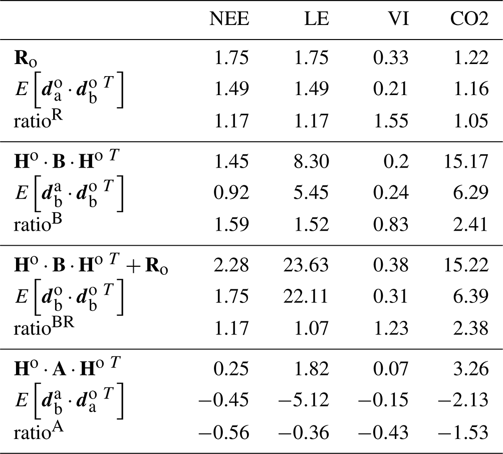
The diagnostics for R_o (ratios slightly above 1 for all data streams) and for the reduced chi-square (Table S1 in the Supplement – values below 1) indicate a slight overestimation of the observation error. The diagnostics for B (ratio^B) show a stronger overestimation of the a priori error for NEE, LE and atmospheric CO₂ but an underestimation for NDVI. For fluxes and satellite data, the combined diagnostics for R_o and B (ratio^BR) appear consistent with ratios close to 1. For CO2 however, the value of ratio^BR close to the value of ratio^B highlights the strong influence of the background information (B matrix) or of the model structure on the optimization, while the large value of χ² expresses a strong underestimation of the observation error. Indeed, when determining ${\mathbf{R}}_{{\mathrm{CO}}_{\mathrm{2}}}$, we purposely did not account for the large bias (by about 1 ppm yr⁻¹) between the observed CO₂ temporal profiles at stations and the prior simulations, which is due to the initialization of ORCHIDEE's carbon pools (which is discussed in the Results section).

Finally, for the diagnostics on the analysis, the various tests performed (Sect. S3) all lead to negative quantities. Instead, the simulations of the calibrated model were expected to be contained in between their prior state and the observations (the residuals having opposite signs; their product is positive). This result may reflect too strong a model correction. However, it should be noted that a strong assumption associated with these tests concerns the linearity of the model, which may not hold for terrestrial biosphere models.

2.4 Diagnostics for system evaluation

2.4.1 Optimization performance

We measured the efficiency of any assimilation by quantifying the reduction of the cost function as the ratio of the prior to posterior values. It should be noted that the minimum value of the cost function is not expected to be zero given the uncertainty in both the data and model and the limited number of degrees of freedom (number of optimized parameters) allowed. We also looked at the ratio of the norm of the gradient between the prior and posterior misfit functions, as it illustrates the progression towards the expected optimum, for which the gradient is null. The decrease of the norm of the gradient depends on the estimation problem (nonlinearities, number of observations versus number of optimized parameters, constraints of the data on the model processes, etc.); However, based on our experience with nonlinear problems, we still expect the norm of the gradient to be reduced by at least 2 orders of magnitude.

The analysis of the optimization performances is summarized in Sects. 3.1 and S4.

2.4.2 Model improvement and posterior predictive checks

The model improvement was quantified by the reduction of the RMSD between the model and data, prior and posterior to optimization, expressed in a percentage, as $\mathrm{1}\times (\mathrm{1}-{\mathrm{RMSD}}_{\mathrm{post}}/{\mathrm{RMSD}}_{\mathrm{prior}})$.

We conducted posterior predictive checks by running the model optimized after assimilation of one or two data streams and quantifying the resulting model improvement with respect to the data streams not accounted for in the assimilation.

2.4.3 Uncertainty reduction on parameters and error budget

The knowledge improvement on the model parameters brought by assimilation was assessed by the uncertainty reduction determined by $\mathrm{1}-{\mathit{\sigma }}_{\text{post}}/{\mathit{\sigma }}_{\text{prior}}$, where σ_post and σ_prior are the standard deviation derived from the posterior (A) and prior (B) covariance matrices on the model parameters and output variables.

A comprehensive quantification of the uncertainty reduction on model variables would require accounting also for the covariance matrix of the model structural error, which could be the dominant factor. Because this covariance matrix is difficult to estimate for complex process-based terrestrial biosphere models (see Kuppel et al., 2013, for a first attempt in the case of the NEE), we instead analyzed the posterior errors on NEE and gross primary productivity (GPP) at regional to global scales, as the projection of the posterior error on parameters in the space of the model variables. The posterior error on C fluxes is then characterized by the covariance matrix R^a as

$$\begin{array}{}\text{(9)}& {\mathbf{R}}^{\text{a}}={\mathbf{H}}^{\text{o}}\cdot \mathbf{A}\cdot {\mathbf{H}}^{\text{o}T},\end{array}$$

with the Jacobian matrix H^o being the first derivative of the target quantity (e.g., NEE, GPP) to the optimized parameters derived from an assimilation experiment o.

2.4.4 Assessment of the information content of each data stream

For the joint assimilations using the three different data streams, we further analyzed the influence matrix S that quantifies their leverage on the model–data fit (Cardinali et al., 2004):

$$\begin{array}{}\text{(10)}& \mathbf{S}={\mathbf{R}}^{-\mathrm{1}}\cdot {\mathbf{H}}^{\text{o}}\cdot \mathbf{A}\cdot {\mathbf{H}}^{\text{o}T}.\end{array}$$

A diagonal element S_ii is the rate of change of the simulated observable i with respect to variations in the corresponding assimilated observation i. S_ii is referred to as “self-sensitivity” of “self-influence”. A zero self-sensitivity indicates that this ith observation does not contribute to improving its simulation by the model, whilst S_ii=1 indicates that the fit of the sole observation i mobilizes an entire degree of freedom (i.e., one parameter). In addition to the total influence matrix (Eq. 10), we also determined the partial influence matrices associated with each data stream o, using the corresponding diagonal R_o matrices and in Eq. (10).

We analyzed the trace (i.e., the sum of all diagonal elements, and denoted tr hereafter) of S that quantifies a measure of the amount of information that can be extracted from all observations/all data streams. We used two derived quantities: the global average observation influence (OI) and the relative degrees of freedom for signal (DFS) associated with the data stream o, which measures its relative contribution to the fit. They are defined as follows (with m the total number of observations):

$$\begin{array}{}\text{(11)}& \text{OI}={\displaystyle \frac{\text{tr}\left(\mathbf{S}\right)}{m}}\end{array}$$

and

$$\begin{array}{}\text{(12)}& \text{DFS}=\mathrm{100}\times {\displaystyle \frac{\text{tr}\left({\mathbf{S}}_{\text{o}}\right)}{\text{tr}\left(\mathbf{S}\right)}}.\end{array}$$

3 Results

3.1 Model improvement for the different assimilation experiments

3.1.1 Cost function reduction

The reduction of the cost function varies between the different experiments, with the lowest reductions for the single data streams experiments F and VI (around 10 %). However, the correction of the model–data misfit when CO₂ data are assimilated is much higher (at least factor of 10 reduction). It is noteworthy that this strong model improvement is obtained for a lower departure of the parameters from their prior values than when fluxes or satellite data are assimilated (see Sect. 3.3 and Fig. 6).

A detailed description of the optimization performances with respect to the minimization of the cost function is given in Sect. S4 and Table S2.

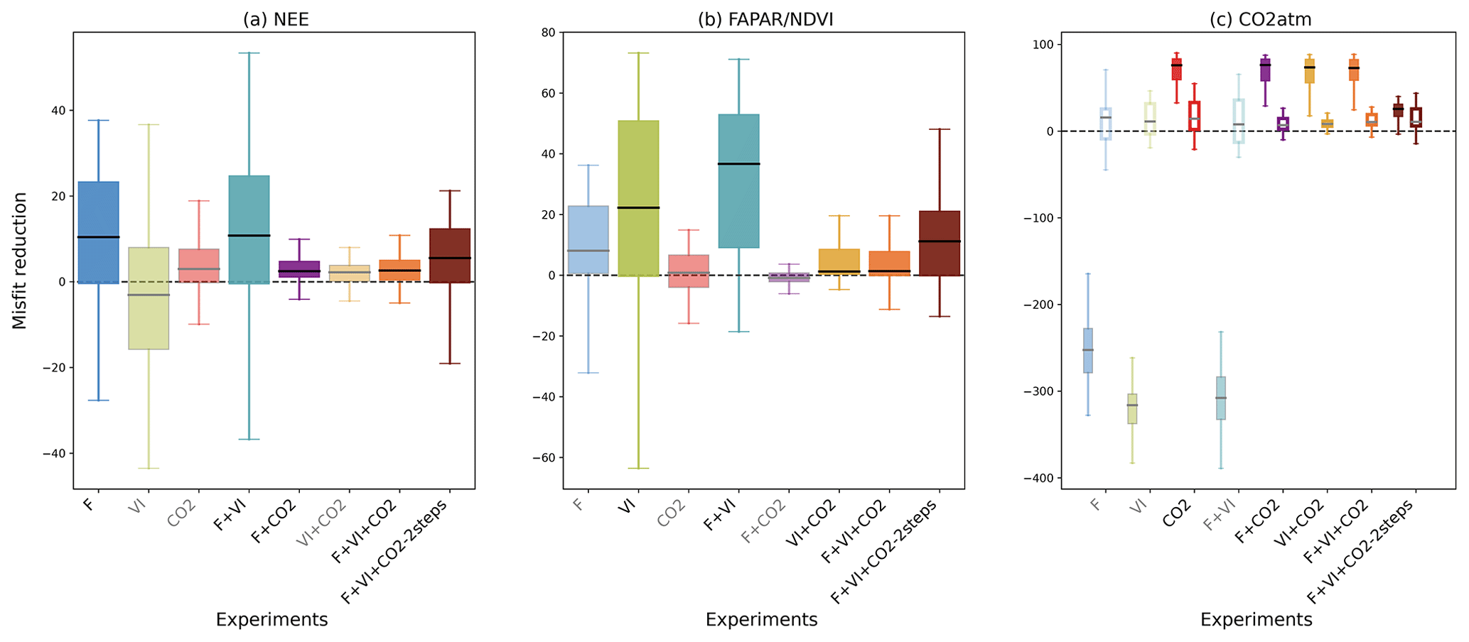
Figure 2 For all data streams, boxplots of the reduction of the model–data mismatch following the different assimilation experiments. For a given data stream, the assimilation experiments in which it is involved are labeled in black (x axis) and the boxplot colors are dark-colored and in gray/light colors otherwise (back-compatibility check). For the atmospheric CO₂ concentration data at stations, the misfit reduction is calculated both for the raw (not detrended) data (left solid boxplot of each assimilation experiment, with colored boxplots) and the detrended data (right white boxplot of each assimilation experiment).

3.1.2 Overall fit to the observations

The impact of assimilating one type of observation on all the data streams (including those that are not assimilated) was evaluated for the various assimilation experiments. The reduction of the model–data mismatch (i.e., reduction in prior RMSD) after assimilation of each data stream (or any combination of them) is illustrated in Fig. 2. The length of the boxes (first and third quartiles) of the whisker plots highlights the spread in misfit reduction across sites/vegetation types. For fluxes, only the impact on NEE is shown, given the choice of the parameters optimized parameters is mostly related to the carbon cycle. Using the parameter values optimized in either the F or VI assimilations has a strong detrimental impact on the simulated atmospheric CO₂ data because the soil carbon pools were not adjusted in these DA experiments. Therefore, we also analyzed the changes induced on the detrended seasonal cycles of atmospheric CO₂ concentrations (Fig. 2c) (hence removing the trend using the time series decomposition based on the CCGCRV routine; Thoning et al., 1989 – see Sect. S2 and Fig. S1 for representative comparisons of observed vs modeled time series of atmospheric CO₂ concentrations and their associated trend estimation).

For a given data stream, the improvement is usually better for the experiment where that data stream is assimilated alone. One noteworthy exception is the assimilation of NDVI alone (VI experiment where only the phenology parameters are optimized) that results in a lower model improvement with respect to NDVI than when it is assimilated in combination with other data streams (where a higher number of parameters are optimized in these joint assimilations, hence improving the timing of phenology and the amplitude of the annual cycle when flux or atmospheric CO₂ data are also assimilated). For both experiments F and VI, the reduction of the model–data misfit can be negative, which reflects how the assimilation can degrade the model performance for a few pixels/sites by searching for a common parameter set. This is not observed with the assimilation of atmospheric CO₂ data, which is the only experiment for which the optimized model is always closer to the observations than the prior model (due to a correction of the CO₂ trend), at all stations (see Sect. S5 for a detailed description of the reduction in model–data misfit for each single data stream assimilation experiment (F, VI and CO2)).

The collateral impact of assimilating one data stream on the other simulated observables is evident in the misfit reductions shown in Fig. 2 (e.g., examine the “VI” experiment on the NEE misfit reduction in Fig. 2a). While using optimized phenological parameters retrieved from satellite data alone (experiment VI) degrades the modeled seasonality of NEE as compared to the measurements (median RMSD reduction of −3 %), the optimization with respect to in situ flux data (F), with additional control parameters, leads to a general improved consistency between modeled FAPAR and satellite NDVI time series (median RMSD reduction of 8 %). The impact on LE is much lower for all DA experiments (median values close to 0 % in all cases, result not shown). One can also note the positive impact of the F and VI assimilations on the atmospheric CO₂ data with median RMSD reductions of 15.8 % and 11.2 % respectively for the detrended time series. Such an improvement after assimilation of in situ flux data corroborates the findings of Kuppel et al. (2014) and Peylin et al. (2016). It is noteworthy that this improvement is of the same order as that achieved when assimilating atmospheric CO₂ data alone (median RMSD reduction of 14 %). The parameters retrieved from the CO2 experiment also have a small but positive impact at the site level with respect to NEE (median value of 3 %) and FAPAR (0.8 %).

For the joint assimilation experiment (F + VI, F + CO2, VI + CO2, or F + VI + CO2; Fig. 2), the model–data agreement is improved for all assimilated data streams, as expected, while the model degradation relative to the data not assimilated is generally not as severe as compared to the assimilation of individual data stream experiments described above, with the exception of the F + VI experiment. The latter experiment leads to enhanced model improvement compared to when flux and satellite NDVI data are assimilated alone (see Sect. S5). In the simultaneous assimilations involving atmospheric CO₂ data, most of the model improvement concerns CO₂ (Fig. 2c), while the benefit for the fluxes and FAPAR/NDVI is weak (RMSD reduction below 3 %). It is noteworthy that the two-step assimilation F + VI + CO2 (see Sect. 2.3.3) results in an even higher model improvement for both NEE and FAPAR than the one-step approach.

The misfit reduction for the raw (i.e., not detrended) atmospheric CO₂ data is high (median reduction ∼75 %) and remains quite stable among the various different combinations of data streams that include atmospheric CO₂ (Fig. 2c solid bars show experiments including “CO₂”), with the exception of the F + VI + CO2-2 steps experiments. The misfit reductions for the detrended CO₂ time series are generally lower (median reduction less than ∼15 %), and there are more pronounced differences between experiments.

These results and the low reduction in NEE and FAPAR RMSDs following the assimilation atmospheric CO₂ data described above highlight the predominance of the correction of the trend in atmospheric CO₂ time series through the fitting of the carbon pool parameters, over the tuning of the other model parameters related to photosynthesis and phenology (see Figs. 6 and S2). The two-step approach permits that limitation to be partially overcome, with the improvement of the mean seasonal cycle for the three data streams (Fig. 2).

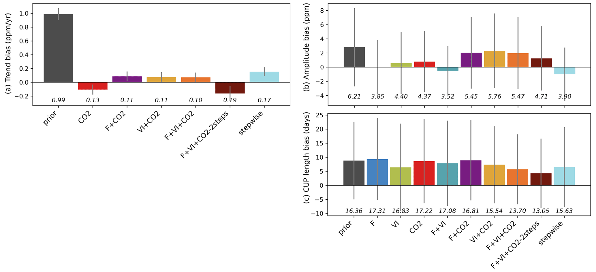
Figure 3 Residual biases of the atmospheric CO₂ time series between those measured at stations and the simulations (prior and optimized for each assimilation experiment), in terms of trend, magnitude of the seasonal cycle and length of the carbon uptake (CUP). The study results are compared to those obtained using a sequential approach (Peylin et al., 2016). The bars show for each quantity the mean bias relative to the measurements over the period 2000–2009. The standard deviations of the differences between observations and simulations over all stations are shown as the vertical gray lines, and the RMSDs are provided below in italic.

3.1.3 Specific improvements at CO₂ stations

Figure 3 further analyzes the impact of each assimilation experiment on the fit to the observed atmospheric CO₂ concentrations in terms of the bias in the long-term trend (2000–2009) and fit to the mean seasonal cycle over the same period (i.e., bias in seasonal amplitude and length of the carbon uptake period – CUP – Sect. S2). For the trend analysis (Fig. 3a), only experiments where atmospheric CO₂ measurements were assimilated are considered.

With the default (prior) parameter values, the fluxes simulated by ORCHIDEE and transported by LMD_Z overestimate the trend by about 1 ppm yr⁻¹. When assimilating atmospheric CO₂ data, most of the parameter correction aims at reducing this bias. This is mostly achieved by tuning the regional K_soilC,reg parameters: The net land carbon sink is increased globally in order to match the observed trend at most stations (reducing the bias from around 1 ppm yr⁻¹ to 0.1 ppm yr⁻¹). Compared to the improvement in the bias in the trend, the improvements (reduction in bias) in the amplitude of the CO₂ seasonal cycle and in the length of the carbon uptake period (CUP) (Fig. 3b and c) are marginal. Note that our joint DA experiments lead to lower trend biases compared to the stepwise approach.

For the amplitude of CO₂ concentrations, the joint assimilations including CO₂ data lead to lower improvements on average compared to any single data stream assimilation experiment. Interestingly, the highest improvements in CO₂ amplitude are achieved when flux data are assimilated (F or F + VI), which reveals that the constraint on photosynthesis and respiration provided by FLUXNET measurements is consistent with the amplitude of the seasonal atmospheric CO₂ cycle and within the ORCHIDEE-LMDz model (as already pointed out in Kuppel et al., 2014). Surprisingly, the use of satellite vegetation indices (VI) leads to a slightly lower residual amplitude bias than when atmospheric CO₂ data are assimilated, albeit a lower number of optimized parameters. For the length of the CUP, the relative model correction appears small for almost all experiments and is lower than what is achieved for the trend and amplitude. Some degradation (increased model–data bias) is even obtained for the cases F and F + CO2. This may be attributed to some inconsistency in the phasing of the CUP derived from the FLUXNET stations and from the atmospheric stations (given differences in the spatial- and temporal-scale constraints brought each data stream). Among the single data stream assimilations, the highest improvement is obtained for VI, where the optimization of the phenological parameters was the only improvement allowed for tuning the model. For the joint assimilations, those combining the three data streams provide the best performance and perform better than the stepwise approach.

Among the joint assimilations with three data streams, the two-step approach results in the largest reduction in amplitude and CUP bias but, on the other hand, the larger trend bias.

3.2 Impact of the assimilations on regional to global land C fluxes and errors

Figure 4 now compares the carbon fluxes (NEE and GPP) at the global scale and for three large regions (northern and southern extratropics and tropics) using hindcast simulations based on the different optimizations.

NEE is close to equilibrium by construction in the prior model (about −0.3 GtC yr⁻¹ globally). Note first that experiments excluding CO₂ data produce land carbon fluxes that are not compatible with our understanding of the land C fluxes (from −10 (F + VI) to +6 (VI) GtC yr⁻¹, not shown in Fig. 4). For all experiments including atmospheric CO₂ data, the assimilations lead to much more negative NEE (increased land carbon sink) compared to the prior for nearly all regions: the optimized carbon sinks are about −2.4 GtC yr⁻¹ at the global scale, similar to the stepwise approach (see Sect. S6 for detailed results for each assimilation experiment). Therefore, our joint assimilations with atmospheric CO₂ data result in a land C sink that is in the range of independent TBM estimates of the global net carbon budget (over the same period, the Global Carbon Project reports a global land sink of −2.9 GtC yr${}^{-\mathrm{1}}\pm \mathrm{0.8}$ standard deviation; see Table 5 of Friedlingstein et al., 2020). Note that we have imposed (see method in Sect. 2.1.2) a net emission from land use change (i.e., deforestation) of +1.1 GtC yr⁻¹ (2000–2009), which is slightly lower than that reported in Friedlingstein et al. (2020) from the TBMs (1.6±0.5 GtC yr⁻¹) or the Bookkeeping methods (1.4±0.7 GtC yr⁻¹), hence our lower terrestrial carbon sink.

These similar posterior global-scale budgets however hide large regional contrasts. While the three joint assimilation experiments F + CO2, VI + CO2 and F + VI + CO2 lead to similar NEE budgets across regions (with magnitudes comparable to the stepwise assimilation setup), the CO2 and F + VI + CO2-2steps experiments result in distinctly different estimates. In the northern extratropics, the CO2 assimilation results in the largest C sinks (numbers provided in Sect. S6) while the F + VI + CO2-2steps assimilation leads to the lowest C sink. The reverse is obtained for the tropics.

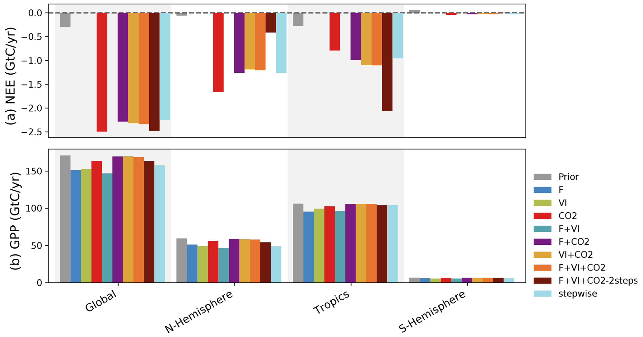
Figure 4 Global and regional C budget for NEE and GPP and for the Northern Hemisphere (30–90^∘ N), tropics (30^∘ N–30^∘ S) and Southern Hemisphere (30–90^∘ S) regions, for the prior model and the model calibrated for the several assimilation experiments. For NEE, only the experiments involving atmospheric CO₂ data are shown. The period considered is 2000–2009.

With a global-scale budget of 171 GtC yr⁻¹ for GPP, the prior ORCHIDEE model is on the high range of recent estimates of the global GPP, as synthesized in Anav et al. (2015), the mean value of which is around 140 GtC yr⁻¹. Depending on the data assimilated in this study, the posterior GPP ranges from 147 GtC yr⁻¹ (F + VI) to 170 GtC yr⁻¹ (VI + CO2) at the global scale. The largest differences with the prior are obtained for the experiments involving flux and satellite data (alone or the two combined). This is directly linked to large corrections in photosynthesis and phenology parameters for these experiments (see Sect. 3.3). In comparison, the assimilations involving atmospheric CO₂ concentration data are more conservative with respect to GPP. Assimilating atmospheric CO₂ data alone lessens the GPP reduction by a factor of about 3 compared to assimilations with F and VI data, and the correction for the joint assimilations using CO₂ data is even lower (see Sect. S6 for details).

By propagating the error on the parameters in the observation space (see Eq. 9), we calculated the uncertainty in NEE and GPP fluxes caused by parameter uncertainty for the prior and optimized models. The error statistics, initially calculated at monthly/grid-scale resolutions, were aggregated over the same regions as above, fully accounting for the spatiotemporal correlations between grid cells (Fig. 5).

At the global scale, the prior error standard deviation for NEE (4.7 GtC yr⁻¹) is high compared to the typical uncertainty associated with TBMs (about 0.5 GtC yr⁻¹, Friedlingstein et al., 2020) or to atmospheric inversions (estimated uncertainty ∼0.4 GtC yr⁻¹ in Peylin et al., 2013). This is a consequence of neglecting negative error correlations between them (as done in nearly all C cycle DA studies). Given this high prior uncertainty, the posterior error for NEE and GPP is significantly reduced, as expected. Because of the strong dependence of the posterior errors on the optimization setup and the fact we do not consider the error of the model, we should only compare the relative error reduction between DA experiments. It is noteworthy that the posterior errors in global NEE obtained for the experiments CO2 and VI + CO2 are about 15 times lower than the posterior errors resulting from the other data combinations (and three orders of magnitude lower than the prior error). This is due both (i) to the need for the DA system to correct the large a priori mismatch of the atmospheric CO₂ growth rate and (ii) to the lower number of optimized parameters in these configurations (Table 2: about 60 % more parameters being optimized in F + VI + CO2 than in CO2 or VI + CO2). The joint assimilations result in higher posterior errors on NEE, while they usually lead to the lower posterior errors on GPP. For GPP, the lowest posterior errors are found for the experiments combining F and CO2 data, while experiments F, CO2 and VI + CO2 lead to larger posterior errors. This is due to the fact that (i) F and CO₂ data provide a stronger constraint on the annual mean photosynthesis than VI data and that (ii) F and CO₂ data provide cross constraints on photosynthesis. Experiment VI, in which about 10 times fewer parameters are optimized and targeting primarily the timing of phenology, results in the highest posterior GPP errors (although still a reduction from the prior).

Finally, one can observe that the posterior errors are higher in the tropics for both NEE and GPP (and the reduction compared to the prior error is lower), which is even more prominent in the experiments using in situ flux data alone or with satellite data, a direct consequence of the lower data availability (eddy-covariance measurements) to constrain the model parameters for tropical PFTs.

3.3 Parameter estimates and associated uncertainties

Figure 6 shows the impacts of the different assimilation experiments on a subset of the retrieved parameter values and their associated uncertainties (the remaining parameters are shown in Fig. S2).

While the stepwise study showed only few changes in the parameter estimates between the sequential steps (and hence as a function of the data stream from which the parameters were constrained) (Peylin et al., 2016), our results show a large variability between the assimilation experiments. For most parameters, the highest departures from the prior values are obtained for the single data stream assimilations. Higher changes are obtained for flux or satellite data as compared to the estimates retrieved with atmospheric CO₂ data alone which remain closer to the prior values. This reflects the lower constraint brought by the CO2 assimilation experiment on photosynthesis- and phenology-related processes, as already pointed out in Sect. 3.1.2. This is largely due to the correction of the trend bias via a few respiration-related parameters, which prevails over the improvement of the other photosynthesis and phenology parameters.

The joint assimilations usually result in a lower departure from the background. For the parameters constrained by two data streams, the optimized values generally fall in between those retrieved when these data streams are assimilated alone. This feature shows how the system tries to find a compromise solution and illustrates potential overfitting with only one data stream. The values optimized in the three experiments involving atmospheric CO₂ data show little variability for all parameters, except in F + VI + CO2-2steps where the tuning of the multiplicative parameter of regional soil carbon pools K_soilC,reg is decoupled from the optimization of the other photosynthesis and phenological parameters. The decrease of K_soilC,reg parameters from the prior value is very small in all experiments, although these parameters are responsible for most of the correction of the atmospheric CO₂ trend. This highlights the challenge of optimizing soil C disequilibrium with our approach based on a model spin-up followed by only a short transient period. The smallest K_soilC,reg changes are obtained for the two-step approach. Note that in this approach, Q₁₀ is also estimated in the first step; the corresponding estimate is similar to the value retrieved in the second step (which is displayed in Fig. 6), with below 0.5 % difference, and consistent with the estimates of the other joint assimilation experiments. For some parameters/PFTs, the direction of the departure with respect to the prior value (increase or decrease) may differ depending on the data stream assimilated.

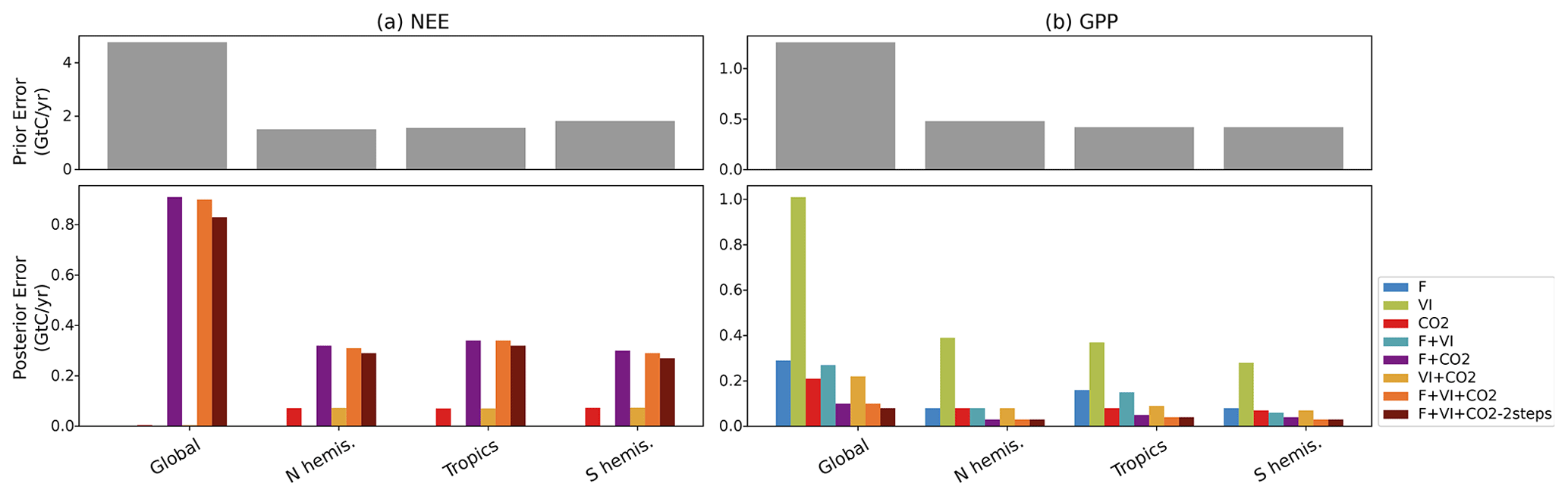
Figure 5 For NEE (a) and GPP (b) prior errors (top) and posterior errors obtained for each assimilation experiment (bottom), over the regions considered. For NEE, only the experiments involving atmospheric CO₂ data are shown.

At the first order, the estimated parameter uncertainties decrease with the number of observations assimilated, as expected from Eq. (3), and given that the observations are treated as independent data. However, given that the estimated parameter errors strongly depend on the setup of B and R matrices and that we did not use error correlations in these matrices, we should only focus on the relative error reduction between experiments. The uncertainty reduction achieved through the assimilation of atmospheric CO₂ data is usually lower than when flux and satellite data are assimilated alone and typically varies between 10 % and 60 % for most photosynthetic and phenological parameters. Most often, the joint assimilations involving two data streams result in an uncertainty reduction higher or of the same order than that achieved in the single data assimilations. The joint assimilation combining the three data streams generally results in the highest uncertainty reduction, with values typically between 60 % and 90 %. The values are much higher than those inferred from the stepwise approach, which are more on the order of the uncertainty reduction obtained in the CO2 assimilation experiment.

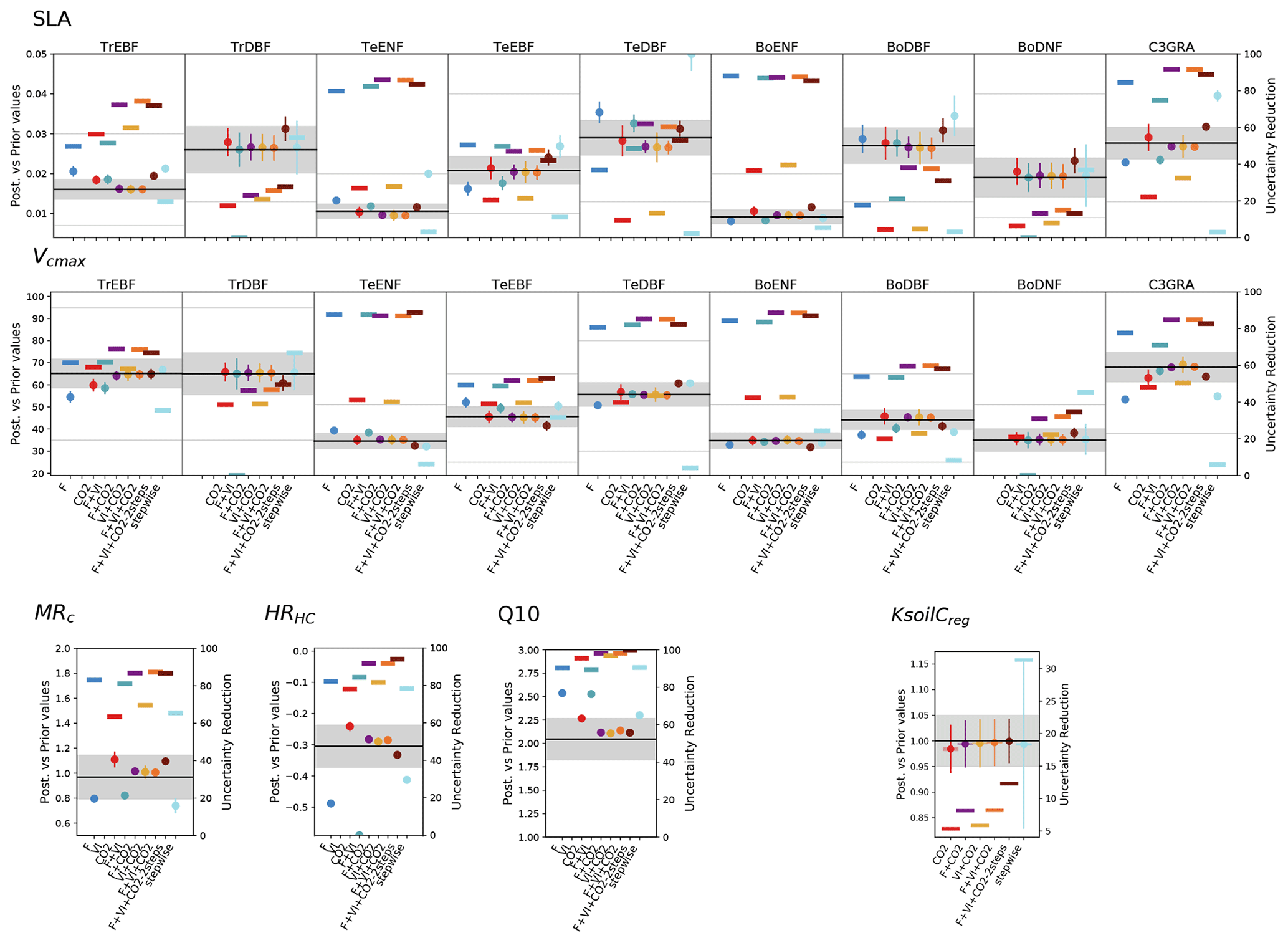
Figure 6 Prior and posterior parameter values and uncertainties for a set of optimized parameters (two PFT-dependent parameters – SLA and V_cmax – and four non-PFT-dependent). The prior value is shown as the horizontal black line and the prior uncertainty (standard deviation) as the gray area encompassing it along the x axis. For the PFT-dependent parameters, each box corresponds to a given PFT; empty boxes indicate that this parameter was not constrained for the corresponding PFTs. The white zone (non-dashed area) corresponds to the allowed range of variation. The optimized values are provided for each assimilation experiment (the eight ones considered in this study and the one from Peylin et al. (2016) – “stepwise”); the corresponding posterior errors are displayed as the vertical bars. For each assimilation experiment the uncertainty reduction is also provided (right y axis) as the thick opaque horizontal bars. For K_soilC,reg, the posterior values displayed here correspond to the mean over the ecoregions (without Antarctica) considered; the semi-transparent horizontal bars on either side of the posterior values correspond to the standard deviation of the estimates.

3.4 Relative constraints brought by the different datasets

We now quantify the impact of each of the three data streams on the analysis using the global average observation influence (quantified by OI) and information content (DFS) metrics defined in Sect. 2.4.4. We recall that OI (i.e., trace of S normalized by the number of observations) gauges the average influence that each single observation has on the analysis, while the relative DFS measures the overall weight of one data stream in the optimization (the difference between OI and DFS is due to the number of observations assimilated; Cardinali et al., 2014). OI and DFS are determined for the joint assimilation experiments combining the three data streams.

Because of the very large number of observations (above 300 000) involved in the assimilation, only the diagonal elements of the influence matrix (Eq. 10) can be calculated. The trace of S measures the equivalent number of parameters and is equal to 132. Such a value, lower than the number of parameters (182), indicates that the optimized parameters may not be fully independent (although parameter error correlations have been ignored in our B matrix) as already reported in Kuppel et al. (2012) or that some are not constrained during the optimization process (as for instance LAI_MAX, whose estimate remains at its a priori value for some PFTs; Fig. S2).

Table 4 Observation influence and relative DFS statistics of each data stream for the joint assimilation experiments F + VI + CO2 and F + VI + CO2-2steps.

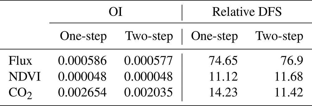
The values of OI are provided in Table 4 for flux, NDVI and atmospheric CO₂ data. With about the same number of observations considered (Table 2, last column), one in situ flux measurement has about 10 times more weight than one NDVI observation. This is a consequence of the larger number of parameters constrained by flux measurements than by NDVI data in our setup. The highest influence is found for atmospheric CO₂ data, the relative weight of one atmospheric CO₂ measurement being 4 times larger than that of one flux observation, despite the much lower number of data assimilated. Again, this is a consequence of the large weight of the mismatch between the a priori-simulated trend and the observed trend in the atmospheric CO₂ data, which is drastically reduced through the optimization.

However, the smaller number of atmospheric CO₂ data assimilated, compared to flux and NDVI datasets, reduces the overall constraint on the analysis provided by atmospheric CO₂ data, as gauged by its relative DFS. Hence, our optimization is mainly controlled by flux data, which have an overall contribution of about 75 %, which is about 5 times larger than the constraint brought by atmospheric CO₂ data and 7 times larger than that of satellite NDVI. Differences between F + VI + CO2 and F + VI + CO2-2steps are relatively small for both OI and DFS but show a slightly lower weight of atmospheric CO₂ data for the 2 steps experiment. A complementary analysis in which the influence of each PFT and each atmospheric station is differentiated is provided in Sect. S7.

4 Discussion

4.1 Benefits of simultaneous assimilations

Joint/simultaneous assimilations are more complex to implement compared to stepwise/sequential assimilations. In principle, a stepwise approach could lead to similar results to a simultaneous approach, if the posterior parameter error covariance matrix could be fully characterized at each assimilation step and further propagated as prior information in the next step. However, given that this is difficult in practice, and because of model nonlinearities and equifinal solutions, stepwise/joint approaches lead to different optimized models (Kaminski et al., 2012; MacBean et al., 2016). With a joint assimilation, biases and incompatibilities between data streams may impact a larger set of parameters than in a stepwise assimilation more directly. The characterization of the prior observation errors also becomes more critical as they condition the relative weight of the observations in the misfit function to minimize and their influence on the solution (analysis). Here, we designed several tests beforehand to refine the configuration of the framework for the simultaneous assimilations. Relying on consistency metrics of Desroziers et al. (2005), we improved the prior error statistics on the model parameters and checked that they were consistent with both the prior model–data mismatch and the observations errors for the different data streams. In spite of the limitation of their application to nonlinear models like ORCHIDEE, their implementation has proved to be useful and has led to an improved consistency of the optimized models at regional and global scales.

Single data stream assimilations usually lead to the best model–data fit for the assimilated data stream, as compared to joint assimilations. However, most often these single data stream assimilations also produce degraded results with respect to the data that were not assimilated. This reveals potential overfitting issues with a higher variability of the optimized parameter values than in the joint assimilations. Overfitting is a key issue for DA studies, which can be partly alleviated when combining different data streams within a consistent framework: because they bring different information on the model processes, they contribute to better circumscribing a set of model parameters. Among the several assimilation experiments considered, those where several data were assimilated simultaneously were those in which there was always an improvement in optimized variables (i.e., no deterioration in model–data fit). The joint assimilations resulted in a reduced variability in parameter estimates and in optimized NEE and GPP.

4.2 Realism of the regional- to global-scale C fluxes

The overarching objective of the study was more about assessing how to make the best of a synergistic exploitation of different data streams within a consistent assimilation framework rather than achieving an up-to-date reanalysis of the global carbon fluxes, especially since we focused on a limited dataset both in terms of temporal coverage (no atmospheric CO₂ data nor satellite data after 2010, no in situ flux data beyond 2007) and of informational constraint. Indeed, we did not assess the potential of other data that can bring relevant (and possibly more direct) additional constraints on the dynamics of terrestrial carbon stocks and fluxes, such as aboveground biomass (Thum et al., 2017) or solar-induced fluorescence (Bacour et al., 2019b), which have already been investigated with ORCHIDAS and with an updated version of the ORCHIDEE model. The expansion of the assimilated datasets to provide the most up-to-date constraint on modeled carbon fluxes will be the subject of future work.

In spite of these limitations, we saw that the regional-/global-estimated NEE and GPP budgets are realistic and in agreement with independent estimates. There are still important differences in the model predictions for the different assimilation experiments (and we have not attempted to identify what was the most reliable optimized model, which would require the use of an ensemble of independent data, an effort beyond the scope of this paper). Still, our optimized simulations allow for a more in-depth exploration of the partitioning of the land carbon budget between the northern extratropics and the tropics. From the global carbon budget, a discrepancy exists between the partition estimated by the atmospheric CO₂ inversions and by the terrestrial biosphere models (Kondo et al., 2020). Atmospheric inversions estimate a larger sink over the northern extratropics than TBMs (around 1.8 GtgC yr⁻¹ versus 1.0 GtC yr⁻¹ for the period 2010–2020), although with large variations between TBMs (Friedlingstein et al., 2020, Fig. 8). Conversely, TBMs estimate a larger C sink over the tropics (Ahlström et al., 2015; Sitch et al., 2015), possibly due to strong CO₂ fertilization effects in TBMs (Schimel et al., 2015), than the inversions, which estimate an approximately net neutral C sink (Peiro et al., 2022). The F + VI + CO2-2steps assimilation follows the typical partitioning pattern of TBMs' behavior, with a stronger C sink in the tropics than in the Northern Hemisphere (Fig. 4). In contrast, all other multiple data stream experiments with CO₂ included (F + CO2, VI + CO2 and F + VI + CO2) and the stepwise approach lead to an approximately equal C sink in the Northern Hemisphere and tropics (thus unlike the general pattern for TBMs and more in line with atmospheric inversions); and on the other hand, the CO2 experiment leads to a similar regional partitioning as the atmospheric inversions. For the F + VI + CO2-2steps experiment, the tropical sink is almost doubled as compared to the other simultaneous assimilation experiments in spite of a slightly reduced GPP.

4.3 Caveats and perspectives concerning the initialization of the soil carbon pools

We showed that reaching the global terrestrial carbon sink was mostly achieved by correcting the initial soil carbon reservoirs in the ORCHIDEE model. Their tuning enables the correction of the biased trend between atmospheric CO₂ time series measurements at stations and the prior ORCHIDEE-LMDz model. The impact of this biased trend on the optimization performance was highlighted by the quantification of the influence for the three data streams on the optimization, with atmospheric CO₂ data having the largest average observation influence on the solution. A consequence of correcting the biased trend is that the model improvement with respect to other processes (photosynthesis and phenology) is hindered.

From a more general perspective, the detrimental consequences of model–data biases become even more important when assimilating multiple observational constraints because of their interconnected contribution to the model calibration. It should be noted that the impact of systematic model–data errors is not inherent to our minimization approach (gradient-based) and has also been highlighted using random search approaches (Brynjarsdóttir and O'Hagan, 2014; Cameron et al., 2022). Thus, accounting for bias correction approaches in data assimilation schemes (Dee, 2005; Trémolet, 2006; Kumar et al., 2012) is becoming increasingly important as the complexity of models and the number of observational constraints increase.

We attempted to overcome this here by setting up a two-step assimilation process where the trend correction is mostly achieved in the first step by tuning the regional parameters controlling the soil carbon pools. In doing so, the two-step approach optimizes the constraint brought by in situ and satellite data (in the second step) in the joint assimilation process. Therefore, the two-step assimilation results in enhanced model–data consistencies compared to a standard simultaneous assimilation (as observed in Figs. 2 and 3), with a caveat regarding atmospheric CO₂ data (the improved fit is mostly with the detrended atmospheric CO₂ data but not the raw data) and the distribution of the land C sink (we saw above that this experiment tends to favor a tropical C sink). We acknowledge the fact that this method is not optimal and requires further investigation. Going beyond the steady-state assumption following model spin-up has been discussed already (Carvalhais et al., 2010; MacBean et al., 2022), as the steady-state assumption results in biased estimates of soil carbon reservoirs (Exbrayat et al., 2014). Extending the period for the transient simulations following spin-up, like is done in the TRENDY experiment (Sitch et al., 2015), would have led to more realistic soil C imbalance and increased the consistency of the modeled atmospheric data with the measurements. Improving the representation of soil carbon stock trajectories in TBMs is pivotal to predicting NEE in regional to global assessments of the capacity of the terrestrial ecosystems to absorb or not atmospheric CO₂. We used atmospheric CO₂ data here to optimize a scalar that accounts for the soil C disequilibrium. The optimization of scaling factors of soil carbon pools is a handy alternative to the optimization of the parameters controlling the turnover times and soil carbon input of the ORCHIDEE soil C model. This would require the spin-up (over at least 1000 years) and transient simulations to be included in the minimization process at each iteration; the prohibitive calculation times for performing this type of optimization preclude us doing this for now. Exploiting TBM databases more directly related to regional soil carbon contents, such as the Harmonized World Soil Database (HWSD) (FAO/IIASA/ISRIC/ISSCAS/JRC, 2012), the International Soil Carbon Network (Nave et al., 2016) or the global soil respiration database (Jian et al., 2021), is not straightforward because of the errors associated with these datasets (Todd-Brown et al., 2013) and inconsistencies between the estimated quantities and the model state variables and underlying processes (as for instance the depth of the soil carbon). In any case, what is sorely needed is data that track changes in C stocks over long time periods. Still, it is of primary importance for the science community to endeavor to bridge the gap between state-of-the art estimates of soil carbon stocks and the quantities that TBMs simulate over the historical period.

5 Conclusions

By assimilating up to three independent carbon-cycle-related data streams simultaneously or separately (in situ measurements of net carbon and latent heat fluxes, satellite-derived NDVI data, and measurements of atmospheric CO₂ concentration at surface stations) within the ORCHIDEE global model (and an offline transport model based on precalculated transport fields with LMDz), we have been able to analyze their compatibility, complementarity and usefulness, in the frame of a global-scale carbon data assimilation system. To do so, the study relied on different metrics to set up and interpret the assimilation performances. The approach as well as the explored metrics is general enough to benefit a broader set of data assimilation applications, supporting guidance for setting up such a C cycle DA framework and for better use of the data to be assimilated.

We investigated how the different combinations of data streams constrain the parameters of the ORCHIDEE land surface model and by consequence the simulated historical spatial and temporal distribution of the net and gross carbon fluxes (NEE and GPP), as well as FAPAR and atmospheric CO₂ concentrations. We quantified how the combination of these data streams (two by two or all together) impacts the reliability of the model predictions. Although it leads to lower fitting performances with respect to the assimilation of any individual dataset (because the optimization seeks a trade-off solution between all data streams), the simultaneous assimilation of the three data streams is found to be the most consistent approach. In particular, it avoids model overfitting, which can degrade the model predictions with respect to data streams not assimilated. The successive model evaluations performed after the assimilation highlighted challenges in handling model–data bias in Bayesian optimization frameworks.

In this study, we focused on biases associated with the initialization of the soil carbon pools in our setup (the fact that they are out of equilibrium because of all historical land cover change and land management impacts). A careful spin-up including a transient simulation to account for the impact of all past disturbances (climate, land cover and land management) is mandatory but likely not sufficient (due to uncertainties in the historical evolution of these drivers) to achieve accurate simulation of the space–time distribution of the global land C sink. Next steps should focus on including part of the spin-up (i.e., such as the transient simulation) in the assimilation procedure, possibly in conjunction with initial C pool optimization.

Terrestrial ecosystem modelers are anticipating the many novel types of observations that are being made available for model evaluation and assimilation. As a result, and in parallel to the growing complexity of TBMs incorporating new biogeophysical processes related to the carbon and water cycles, new observation operators are being developed to be able to make use of this new wealth of data. With these new perspectives ahead, the global land surface modeling community should investigate some of the issues highlighted in this study and linked to multiple data streams assimilation, initial model state optimization and/or the inclusion of the spin up in the DA system, etc. more deeply in order to achieve significant reduction in land surface model projection uncertainties.