the Creative Commons Attribution 4.0 License.
the Creative Commons Attribution 4.0 License.
 | 12 Apr 2023
Using machine learning and Biogeochemical-Argo (BGC-Argo) floats to assess biogeochemical models and optimize observing system design
Alexandre Mignot
Hervé Claustre
Gianpiero Cossarini
Fabrizio D'Ortenzio
Elodie Gutknecht
Julien Lamouroux
Paolo Lazzari
Coralie Perruche
Stefano Salon
Raphaëlle Sauzède
Vincent Taillandier
Anna Teruzzi
Numerical models of ocean biogeochemistry are becoming the major tools used to detect and predict the impact of climate change on marine resources and to monitor ocean health. However, with the continuous improvement of model structure and spatial resolution, incorporation of these additional degrees of freedom into fidelity assessment has become increasingly challenging. Here, we propose a new method to provide information on the model predictive skill in a concise way. The method is based on the conjoint use of a k-means clustering technique, assessment metrics, and Biogeochemical-Argo (BGC-Argo) observations. The k-means algorithm and the assessment metrics reduce the number of model data points to be evaluated. The metrics evaluate either the model state accuracy or the skill of the model with respect to capturing emergent properties, such as the deep chlorophyll maximums and oxygen minimum zones. The use of BGC-Argo observations as the sole evaluation data set ensures the accuracy of the data, as it is a homogenous data set with strict sampling methodologies and data quality control procedures. The method is applied to the Global Ocean Biogeochemistry Analysis and Forecast system of the Copernicus Marine Service. The model performance is evaluated using the model efficiency statistical score, which compares the model–observation misfit with the variability in the observations and, thus, objectively quantifies whether the model outperforms the BGC-Argo climatology. We show that, overall, the model surpasses the BGC-Argo climatology in predicting pH, dissolved inorganic carbon, alkalinity, oxygen, nitrate, and phosphate in the mesopelagic and the mixed layers as well as silicate in the mesopelagic layer. However, there are still areas for improvement with respect to reducing the model–data misfit for certain variables such as silicate, pH, and the partial pressure of CO2 in the mixed layer as well as chlorophyll-a-related, oxygen-minimum-zone-related, and particulate-organic-carbon-related metrics. The method proposed here can also aid in refining the design of the BGC-Argo network, in particular regarding the regions in which BGC-Argo observations should be enhanced to improve the model accuracy via the assimilation of BGC-Argo data or process-oriented assessment studies. We strongly recommend increasing the number of observations in the Arctic region while maintaining the existing high-density of observations in the Southern Oceans. The model error in these regions is only slightly less than the variability observed in BGC-Argo measurements. Our study illustrates how the synergic use of modeling and BGC-Argo data can both provide information about the performance of models and improve the design of observing systems.
- Article
(3409 KB) - Full-text XML
- BibTeX
- EndNote


Since preindustrial times, the ocean has taken up ∼26 % of total anthropogenic CO2 emissions (Friedlingstein et al., 2022), leading to dramatic change in the ocean's biogeochemical (BGC) cycles, such as ocean acidification (Iida et al., 2020). Moreover, deoxygenation (Breitburg et al., 2018) and change in the biological carbon pump are now manifesting globally (Capuzzo et al., 2018; Osman et al., 2019; Roxy et al., 2016). Therefore, along with plastic pollution (Eriksen et al., 2014) and an increase in fisheries pressure (Crowder et al., 2008), major changes are occurring in marine ecosystems at the global scale. In order to contextualize the monitoring of ongoing changes, derive climate projections, and develop better mitigation strategies, realistic numerical simulations of the oceans' BGC state are required.
Numerical models of ocean biogeochemistry represent a prime tool to address these issues because they produce three-dimensional estimates of a large number of chemical and biological variables that are dynamically consistent with the ocean circulation (Fennel et al., 2019). They can assess past and current states of the BGC ocean and produce short-term to seasonal forecasts as well as climate projections. However, these models are far from being flawless, mostly because there are still huge knowledge gaps in the understanding of key BGC processes and, as a result, the mathematical functions that describe BGC fluxes, and the ecosystem dynamics are too simplistic (Schartau et al., 2017). For instance, most models do not include a radiative component for the penetration of solar radiation in the ocean. Nevertheless, it has been shown that coupling such a component with a BGC model improves the representation of the dynamics of phytoplankton in the lower euphotic zone (Dutkiewicz et al., 2015; Álvarez et al., 2022). Additionally, the parameterization of the mathematical functions generally results from laboratory experiments on a few representative species and may not be suitable for extrapolation to ocean simulations that need to represent the large range of organisms present in oceanic ecosystems (Schartau et al., 2017; Ward et al., 2010). Furthermore, the assimilation of physical data in coupled physical–BGC models that improve the physical ocean state can paradoxically degrade the simulation of the BGC state of the ocean (Fennel et al., 2019; Park et al., 2018; Gasparin et al., 2021). Thus, a rigorous assessment of BGC models is essential to test their predictive skills, examine their ability to reproduce BGC processes, and estimate confidence intervals on model predictions (Doney et al., 2009; Stow et al., 2009).
However, the evaluation of BGC models is limited by the availability of data. It relies principally on a combination of different data sets from satellite observations (such as the chlorophyll a concentration), cruise observations, and permanent oceanic stations from large databases such as the World Ocean Database (e.g., Doney et al., 2009; Dutkiewicz et al., 2015; Lazzari et al., 2012, 2016; Lynch et al., 2009; Séférian et al., 2013; Stow et al., 2009). All of these data sets do not have a sufficient vertical/temporal resolution nor a synoptic view, and they do not provide all of the variables necessary to evaluate how models represent climate-relevant processes such as air–sea CO2 fluxes, the biological carbon pump, ocean acidification, or deoxygenation.
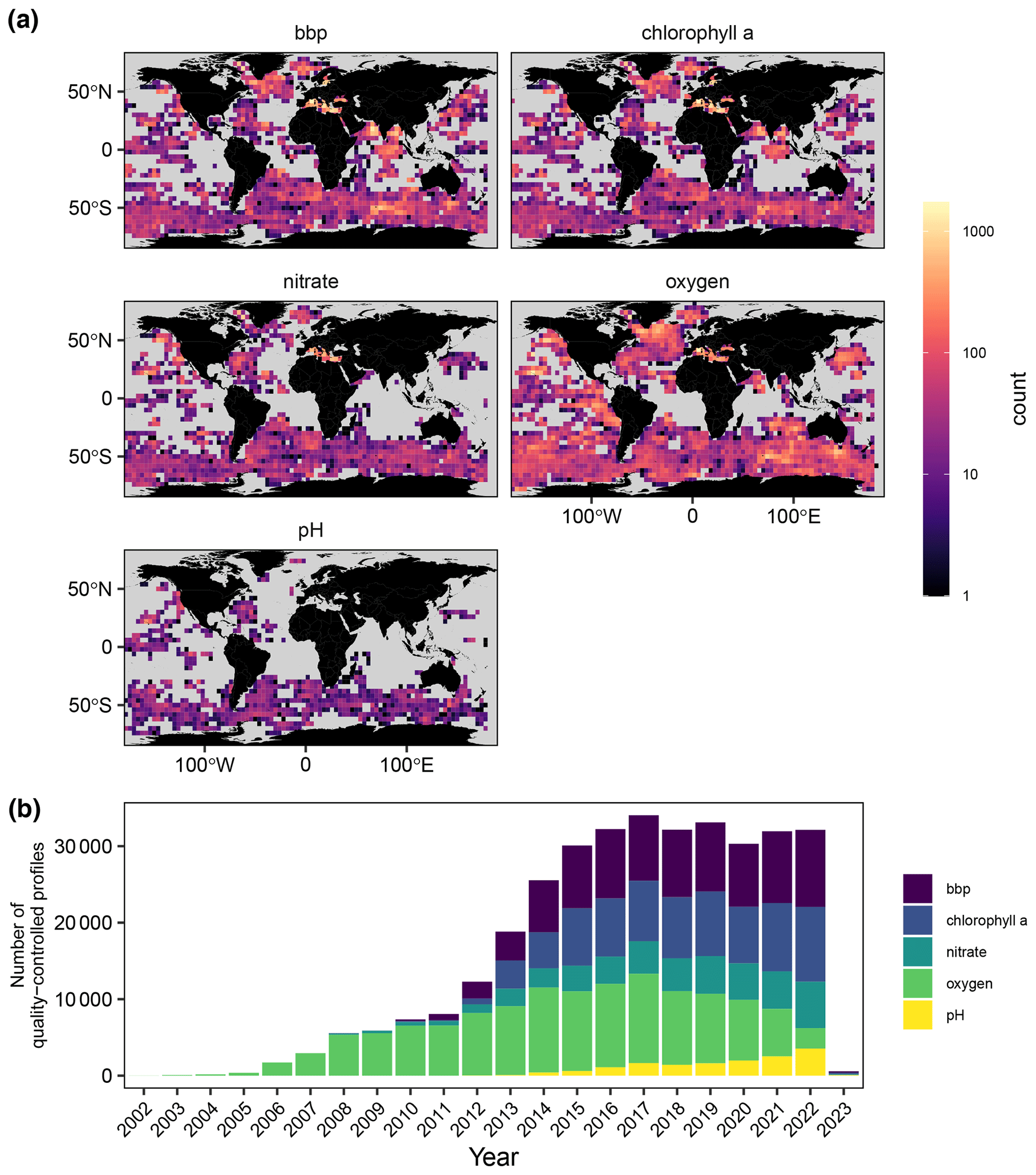
Figure 1Spatial and temporal coverage of BGC-Argo quality-controlled pH, nitrate, chlorophyll a, oxygen, and bbp profiles: (a) the number of quality-controlled profiles for the entire period per 4 bin; (b) the number of quality-controlled profiles per year. Note that this study only uses data from 2009 to 2020 to evaluate model performance.
In 2016, the Biogeochemical-Argo (BGC-Argo) program was launched with the goal of operating a global array of 1000 BGC-Argo floats equipped with sensors measuring the following parameters: oxygen (O2), chlorophyll a (Chl a), and nitrate (NO3) concentrations; particulate backscattering (bbp); pH; and downwelling irradiance (Biogeochemical-Argo Planning Group, 2016; Claustre et al., 2020). Although the planned number of 1000 floats has not been reached yet, the BGC-Argo program has already provided a large number of quality-controlled vertical profiles of O2, Chl a, NO3, bbp, and pH (Fig. 1). With respect to O2, Chl a, NO3, and bbp, the North Atlantic and the Southern Oceans are reasonably well sampled, whereas pH is only well sampled in the Southern Oceans. At the regional scale, the Mediterranean Sea is also fairly well sampled by BGC-Argo floats (Salon et al., 2019; Terzić et al., 2019; D'Ortenzio et al., 2020); however, there are still large undersampled areas like the Arctic Ocean, subtropical gyres, and the subpolar North Pacific. Thanks to machine-learning-based methods (Bittig et al., 2018; Sauzède et al., 2017), floats equipped with O2 sensors can be additionally used to derive vertical profiles of NO3, phosphate (PO4), silicate (Si), alkalinity (Alk), dissolved inorganic carbon (DIC), pH, and the partial pressure of CO2 (pCO2).
The BGC-Argo data set represents a significant improvement for the assessment of models compared with large databases such as the World Ocean Database (Boyer et al., 2013) or the Copernicus Marine Service in situ data set (European Union-Copernicus Marine Service, 2015). Large databases are composed of data collected using various instrument types and heterogenous data sampling methodologies. Therefore, for a given variable, the accuracy numbers are not the same and change depending on the instrument type (European Union-Copernicus Marine Service, 2019). Consequently, the changing proportion of instrument types over the years affects the overall accuracy over time. On the other hand, the BGC-Argo data set is a homogenous data set with strict and uniform sampling methodologies and data quality control (QC) procedures. As a result, the BGC-Argo data set has a satisfactory level of accuracy that remains stable over time (Johnson et al., 2017; Mignot et al., 2019). Moreover, the number of quality-controlled observations collected every year by the BGC-Argo fleet is now greater than any other data set (Claustre et al., 2020). Using the BGC-Argo data set as the single evaluation data set is, therefore, a way to ensure consistent accuracy.
The BGC-Argo floats provide multivariate observations at high vertical and temporal resolutions and for long periods of time, producing nearly continuous time series of the vertical distribution of several biogeochemical variables. This is not possible with the discrete, univariate vertical sampling provided by cruise cast in situ measurements or with climatological values derived from the World Ocean Atlas. All of these specificities overcome the limitations of previous data sets, especially with respect to their univariate nature as well as their limited vertical and temporal resolutions. This opens new perspectives for the evaluation of BGC models (Gutknecht et al., 2019; Salon et al., 2019; Terzić et al., 2019).
The development of BGC models, coupled with the ongoing increase in spatial and vertical resolutions, has resulted in a significant rise in the volume of model output. Simplification techniques are therefore required to provide decipherable information on the model predictive skill. Allen et al. (2007) proposed a methodology to reduce the spatial dimensions in model assessment exercises, thereby providing concise information about the model performance. They used an unsupervised learning algorithm to classify the southern North Sea into five coherent BGC regions based on modeled time series of temperature and NO3, PO4, and Si concentrations. They then evaluated the predictive capability of the model in each BGC region (instead of each grid point), thereby greatly reducing the number of points to be validated. An additional method to reduce the dimensions of model–data comparison is the use of assessment metrics (Hipsey et al., 2020; Russell et al., 2018). In particular, metrics such as depth-averaged state variables (e.g., mixed-layer-averaged Chl a, NO3, and O2), mass fluxes and process rates (e.g., primary production or division rates), or emergent properties (e.g., the deep chlorophyll maximum, DCM, or oxygen minimum zone, OMZ) are particularly useful to reduce the number of model vertical layers to be compared with the observations.
The objective of the present study is twofold. First, we aim to propose a methodology that uses the BGC-Argo data set, an unsupervised learning algorithm, and assessment metrics to simplify marine BGC model–data comparisons and, thus, provides information (in a concise way) about model performance. Second, we aim to use this methodology to identify ocean regions where the model–observation misfit is larger than the variability in the BGC-Argo data and, thus, provide information on regions that should be better sampled by the BGC-Argo observing system. The first step of the method consists of defining 23 assessment metrics that are used both to construct the BGC regions and, subsequently, to compare the model output with the BGC-Argo data. In the second step, following the approach of Allen et al. (2007), we use an unsupervised learning algorithm, specifically a k-means clustering technique, to classify the global ocean into eight coherent BGC regions based on the climatological modeled time series of the 23 assessments metrics. In the last step, the skill of the model with respect to predicting the assessment metrics is evaluated in each BGC region using the model efficiency statistical score. Unlike other statistical metrics such as the correlation coefficient, the bias, or the root-mean-square (RMS) difference, which do not objectively quantify whether the model performance is acceptable or not, the model efficiency calculates whether the model outperforms an observational climatology. Finally, the method is implemented using the global ocean BGC analysis and forecasting system of the Copernicus Marine Service (European Union-Copernicus Marine Service, 2019).
The rest of the paper is organized as follows: Sect. 2 presents the data sets used in this work; Sect. 3 defines the assessment metrics and details the k-means algorithm as well as the model efficiency statistical score; Sect. 4 presents and discusses the results; and, finally, Sect. 5 concludes the study.
2.1 BGC-Argo float observations
The float data were downloaded from the Argo CORIOLIS Global Data Assembly Center in France (ftp://ftp.ifremer.fr/argo, last access: January 2023). The conductivity–temperature–depth (CTD) and trajectory data were quality controlled using the standard Argo protocol (Wong et al., 2015). The raw BGC signals were transformed to biogeochemical variables (i.e., O2, Chl a, NO3, bbp, and pH) and quality controlled according to international BGC-Argo protocols (Johnson et al., 2018a, b; Schmechtig et al., 2015, 2018; Thierry et al., 2018; Thierry and Bittig, 2018).
Table 1Data mode and QC flags of the BGC-Argo observations used in this study. In the Argo data system, the data are available in three data modes: “real time”, “adjusted”, and “delayed”. See Sect. 2.1 for a brief description of each data mode. The flags “3” and “4” refer to “potentially bad data” and “bad data”, respectively. The reader is referred to Bittig et al. (2019) for a more detailed description of the Argo data modes and flags.
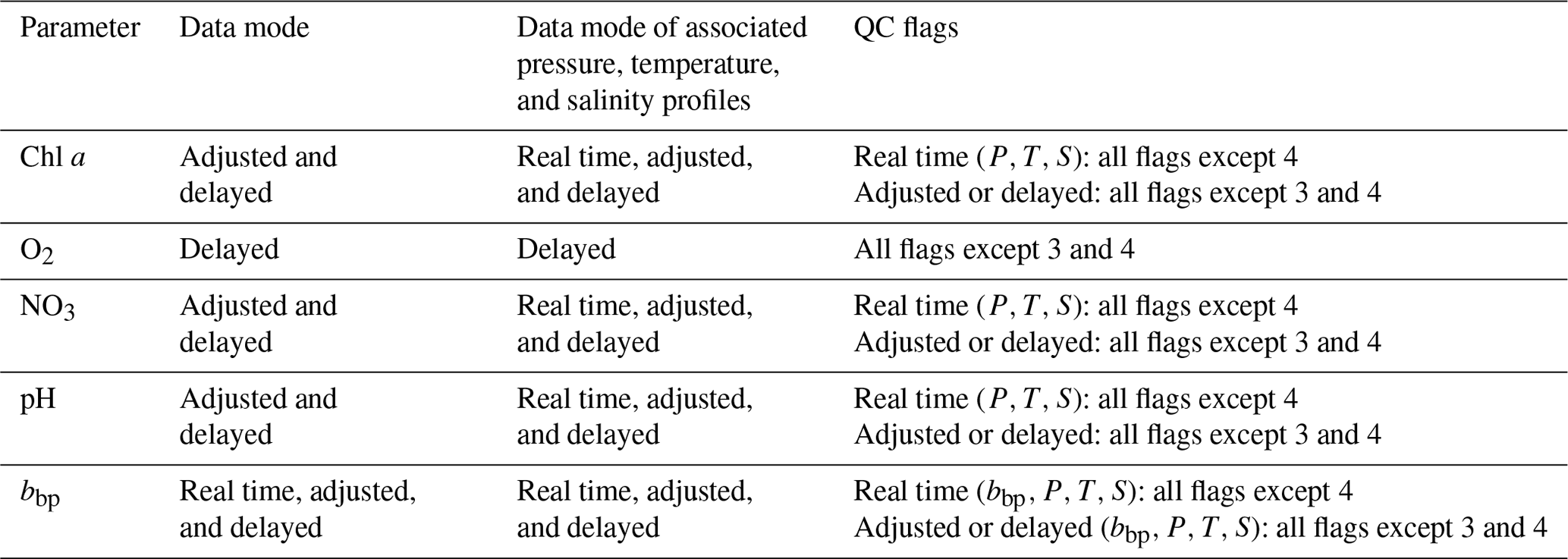
“(P,T,S)” refers to pressure, temperature, and salinity.
In the Argo data system, the data are available in three data modes: “real time”, “adjusted”, and “delayed” (Bittig et al., 2019). In the real-time mode, the raw data are converted into state variables, and an automatic quality control is applied to “flag” gross outliers. In the adjusted mode, the real-time data receive a calibration adjustment in an automated manner. In the delayed mode, the adjusted data are adjusted and validated by a scientific expert. While the real-time and adjusted data are considered acceptable for operational application (data assimilation), the delayed-mode data are designed for scientific exploitation and represent the highest-quality data with the ultimate goal (when time series with sufficient duration have been acquired) of possibly extracting climate-related trends (Bojinski et al., 2014). However, for some variables, only a limited fraction of the data is accessible in the delayed mode. Consequently, for each variable, we selected the highest-level data mode, in which at least 80 % of the data are available (see Table 1). Note that this criterion is not applied to O2, as only delayed-mode data were selected for this variable in order to generate the pseudo-observations from the CANYON-B neural network (more detail given in the following). We removed data with missing location or time information and data flagged as “bad data” (flag = 4). Depending on the parameter and the associated data mode, we also excluded data flagged as “potentially bad data” (flag = 3) (see Table 1). Finally, it should be noted that the status of the different modes of adjustment for bbp is still very inhomogeneous in the global BGC-Argo database. A quality control procedure in real time has just been proposed to the Argo Data Management Team but is not yet operationally implemented in the database (Dall'Olmo et al., 2022). As there is no current official consensus regarding the qualification of bbp data, we decided to use all data modes for this study.
Particulate organic carbon (POC) concentrations were derived from bbp observations. First, three consecutive low-pass filters were applied on the vertical profiles of bbp to remove spikes (Briggs et al., 2011): a two-point running median followed by a five-point running minimum and a five-point running maximum. The filtered bbp profiles were then converted into POC (mgC m−3) using a simplified version of the empirical POC / bbp algorithm developed by Gali et al. (2022), i.e., for depths larger than the mixed-layer depth (MLD):
where c is a constant deep value and b is the slope of the exponential decrease; the aforementioned variables are set to 12 010 mgC m−3 m and −6.57, respectively, as proposed by Gali et al. (2022). The global coefficient a is set to 37 990 mgC m−3 m to be consistent with a relationship, developed for global applications (i.e., POC = 38 (European Union-Copernicus Marine Service, 2020). In the mixed layer (ML), z is fixed at z = MLD, and Eq. (1) simplifies to
Finally, we complemented the existing BGC-Argo data set with pseudo-observations of NO3, PO4, Si, Alk, and DIC concentrations as well as pH and pCO2 using the CANYON-B neural network (Bittig et al., 2018). CANYON-B estimates vertical profiles of nutrients; the carbonate system variables from concomitant measurements of float pressure, temperature, salinity, and O2 qualified in delayed mode; and the associated geolocalization and date of sampling information. CANYON-B was trained and validated using version 2 of the Global Ocean Data Analysis Project (GLODAPv2) data set (Olsen et al., 2016). The CANYON-B estimates of NO3 and pH were merged with measured values based on the rationale that CANYON-B estimates have RMS errors (NO3=0.7 µmol kg−1 and pH = 0.013) (Bittig et al., 2018) that are of the same order of magnitude as those of the BGC-Argo observation errors (NO3=0.5 µmol kg−1 and pH = 0.07) (Mignot et al., 2019; Johnson et al., 2017).
Finally, we verified that the RMS errors in BGC-Argo data (both measured and from CANYON-B estimates) are lower than the RMS difference between the model and BGC-Argo data; therefore, the comparison of simulated properties with the BGC-Argo data leads to a meaningful evaluation of the model performance. We believe it is reasonable to draw conclusions on the model uncertainty from BGC-Argo data as long as the BGC-Argo errors are much lower than the model–observation RMS difference.
2.2 The Global Ocean Biogeochemistry Analysis and Forecast system of the Copernicus Marine Service
The global model simulation used in this study (see Appendix A1) originates from the global ocean hydrodynamic–biogeochemical coupled system, based on the NEMO–PISCES (Nucleus for European Modelling of the Ocean–Pelagic Interaction Scheme for Carbon and Ecosystem Studies) model, implemented and operated by Mercator Ocean for the Copernicus Marine Service within the framework of the European Union's Earth observation program (European Union-Copernicus Marine Service, 2019). The BGC component is constrained by the assimilation of satellite Chl a concentrations, and a climatological damping is applied to nitrate, phosphate, oxygen, and silicate with the World Ocean Atlas 2013, to dissolved inorganic carbon and alkalinity with the GLODAPv2 climatology (Lauvset et al., 2016), and to dissolved organic carbon and iron with a 4000-year PISCES climatological run. The BGC model is forced in offline mode by daily averages of ocean physics, sea ice, and atmospheric conditions. The ocean physics and sea-ice forcing come from the global ocean physics analysis and forecasting system at (Lellouche et al., 2018); the aforementioned system assimilates along-track altimeter data, satellite sea surface temperature and sea-ice concentration, and in situ temperature and salinity vertical profiles. The BGC model has a horizontal resolution with 50 vertical levels (22 levels in the upper 100 m, and the vertical resolution decreases from 1 m near the surface to 450 m near the ocean bottom.
We used the daily output of Chl a, NO3, PO4, Si, O2, pH, DIC, Alk, and pCO2 as well as the weekly output of two size classes of phytoplankton, the small detrital particles and microzooplankton (resampled offline from a weekly to daily frequency via constant interpolation) from 2009 to 2020. Note that the method of linear resampling, which artificially increases the number of data, could potentially bias the statistical results, especially in regions with poor data coverage. As suggested by Gali et al. (2022), the POC concentration was computed offline by adding the two size classes of phytoplankton (the small detrital particles and microzooplankton modeled by PISCES) together. This particular combination of phytoplanktonic and non-phytoplanktonic organisms has been shown to match the small POC observed by the floats. The partial pressures of CO2 values were extrapolated in the mixed layer from the surface value estimated by the model. The Black Sea was not considered in the present analysis because the model solutions are of poor quality. Finally, the daily model output was co-located in time and space closest to the BGC-Argo float positions and was interpolated to the sampling depth of the float observations. The characteristics of the model are further detailed in the Appendix.
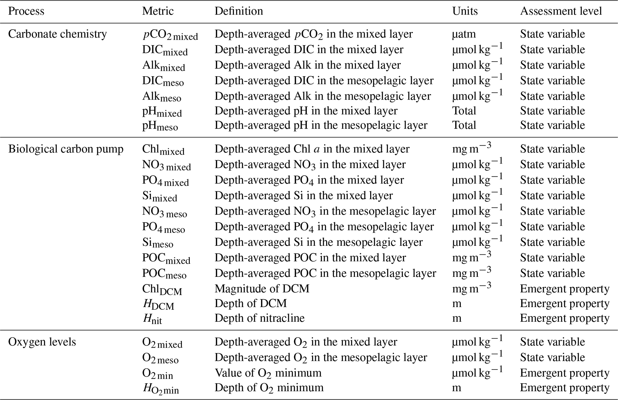
Table 2The metrics used to assess the model simulation with BGC-Argo data. For each metric, the level of assessment, as described in Hipsey et al. (2020), is also indicated.
3.1 Assessment metrics
In this section, we present the 23 metrics used for the clustering of the ocean and for the assessment of the model simulation with BGC-Argo data. The metrics are associated with the carbonate chemistry, the biological carbon pump, and oxygen levels. Most of the metrics evaluate the model state accuracy via the comparison of simulated state variables with BGC-Argo observations that are depth averaged in the mixed (hereinafter indicated with the subscript “mixed”) and mesopelagic (hereinafter indicated with the subscript “meso”) layers. This two-layer comparison between model and BGC-Argo data provides an indirect evaluation of the key processes and fluxes associated with the carbonate chemistry, biological carbon pump, and oxygen levels in the mixed and mesopelagic layers. In addition, some of the metrics assess the skill of the model with respect to capturing emergent properties, such as the nitracline depths, DCMs, and OMZs. The metrics are described below and summarized in Table 2. The definition of the metrics is the same for the model and the BGC-Argo data. The MLD is computed, following De Boyer et al. (2004), as the depth at which the change in potential density (from its value at 10 m) exceeds 0.03 kg m−3. Dall'Olmo and Mork (2014) define the mesopelagic layer as the region between the deeper of either the euphotic layer depth or the MLD and a depth of 1000 m. However, for ease of use, we adopt a simplified definition that considers the mesopelagic layer to be the region between the MLD and a depth of 1000 m. To ensure the accuracy of the metrics' calculation, we have checked the representation of the MLDs in the model. The model's MLDs closely match the observed data, as indicated by an overall mean-square difference of approximately 30 % of the total variance in the observations.
3.2 Carbonate chemistry
The uptake of ∼26 % of anthropogenic CO2 by the global ocean (Friedlingstein et al., 2022) has altered the oceanic carbonate chemistry over the past few decades (Iida et al., 2020). Therefore, assessing how models correctly represent the oceanic carbonate chemistry is critical if we aim to derive accurate climate projections of future change. The classical variables for the study of carbonate chemistry are DIC, Alk, pH, and pCO2 (Williams and Follows, 2011). These variables are assessed in the mixed (DICmixed, Alkmixed, pHmixed, and pCO2 mixed) and mesopelagic (DICmeso, Alkmeso, and pHmeso) layers. The partial pressure of CO2 is only assessed in the mixed layer, as the evaluation of pCO2 mixed plays a critical role in the assessment of BGC models' skill to correctly represent the air–sea CO2 flux.
3.3 Biological carbon pump
The biological carbon pump is the transformation of nutrients and dissolved inorganic carbon into organic carbon in the upper part of the ocean via phytoplankton photosynthesis and the subsequent transfer of this organic material into the deep ocean. The functioning of this pump relies on key pools of nutrients and carbon as well as several processes that control mass fluxes between the pools. Changes in the biological carbon pump are now manifesting globally (Capuzzo et al., 2018; Osman et al., 2019; Roxy et al., 2016).
One way to indirectly evaluate a model's ability to accurately capture essential processes related to the biological carbon pump in the ocean's upper layer, such as primary production, respiration, and grazing, is to compare various ML pools (here the nutrients (NO3 mixed, PO4 mixed, and Simixed), Chlmixed, and POCmixed) with BGC-Argo observations. Similarly, the assessment of the mesopelagic nutrients and POC concentration (hereinafter denoted NO3 meso, PO4 meso, Simeso, and POCmeso) provides an indirect evaluation of the key mesopelagic layer processes, such as export production and respiration.
In stratified systems, a DCM is formed at the base of the euphotic layer (Barbieux et al., 2019; Cullen, 2015; Letelier et al., 2004; Mignot et al., 2014, 2011). It has been suggested that the DCM plays a key role in the synthesis of organic carbon by phytoplankton (Macías et al., 2014). Therefore, DCMs are key features to be assessed in BGC models with respect to processes involved in the biological carbon pump, such as primary production. However, the DCM layer generally escapes detection by remote sensing. Furthermore, the DCM is also an emergent feature that develops in response to complex physical and biogeochemical interactions (Cullen, 2015). Thus, its evaluation provides critical information regarding the accuracy of the model with respect to capturing complex patterns of key ecosystem processes. The depth and magnitude of the DCM (HDCM and ChlDCM, respectively) are helpful metrics for the assessment of DCM dynamics. The depth of the DCM is calculated as the depth where the Chl a maximum occurs in the profile, with the criterion that the HDCM should be deeper than the MLD. The magnitude of the DCM corresponds to the Chl a value at the HDCM.
NO3 is often depleted in the surface layers and is a limiting factor for phytoplankton growth in most oceanic regions. The vertical supply of NO3 to the surface layers depends, among other factors, on the vertical gradient of NO3 (the nitracline) and, in particular, on its depth (the nitracline depth) (Cermeno et al., 2008; Omand and Mahadevan, 2015). Therefore, the comparison of the simulated nitracline depth (Hnit) with BGC-Argo observations allows for an indirect assessment of the model performance with respect to reproducing vertical fluxes of NO3. Following previous studies (Cermeno et al., 2008; Lavigne et al., 2013; Richardson and Bendtsen, 2019), the depth of the nitracline is identified as the first depth where NO3 is detected. A detection threshold of 1 µmol kg−1 is used, which is an upper estimate of the accuracy of BGC-Argo NO3 data (Johnson et al., 2017; Mignot et al., 2019).
3.4 Oxygen levels
Oxygen levels in the global and coastal waters have declined over the whole water column over the past decades (Schmidtko et al., 2017), and OMZs are expanding (Stramma et al., 2008). Therefore, assessing how models correctly represent ocean oxygen levels as well as the OMZs is critical to monitor their change over time. Similar to the assessment of DCMs, evaluating oxygen minimum zones (OMZs) provides insight into how the model represents emergent dynamics resulting from intricate physical and biogeochemical interactions (Paulmier and Ruiz-Pino, 2009). Oxygen levels are evaluated in the mixed (O2 mixed) and mesopelagic (O2 meso) layers. OMZs are defined as oceanic regions where O2 levels are lower than 20 µmol kg−1 (Paulmier and Ruiz-Pino, 2009). OMZs are characterized by their depths (H2 min) and their concentrations (O2 min).
3.5 Bioregionalization of the global ocean
In this study, we use the k-means clustering algorithm (Hartigan and Wong, 1979) to regionalize the ocean based on the modeled climatological monthly time series of the 23 metrics described previously. The k-means clustering algorithm is an unsupervised machine learning technique that groups similar objects together in a way that maximizes similarity between objects within a group and minimizes similarity between objects in different groups. This clustering tool has been successfully used to classify marine BGC regions in different oceanic basins based on the seasonal cycle of satellite chlorophyll (Kheireddine et al., 2021; Mayot et al., 2016; Lacour et al., 2015; D'Ortenzio and d'Alcala, 2009). The step-by-step methodology used in this study is described in the following.
The first step in the analysis involved computing monthly climatological time series for the 23 metrics at each model grid cell. These time series were derived from the monthly climatological time series of state variables predicted by the model from 2009 to 2020. To account for the lognormal distribution and the wide range of values for metrics in units of Chl a or POC, a log-10 transformation was applied to these metrics. Second, to take the 6-month shift in seasons between the Northern and Southern hemispheres into consideration, the dates for grid cells located in the Southern Hemisphere were shifted by 6 months (Bock et al., 2022). Third, to classify model grid cells based on the seasonality and amplitude of the 23 metrics, each metric was standardized by subtracting the global mean and dividing by the global standard deviation. This ensured that each metric had a mean of 0 and a standard deviation of 1, enabling comparison across metrics with different units. Fourth, to reduce the dimensionality of the data set, a principal component analysis was applied to the scaled data. Only the components that explain 99 % of the variance in the data set were kept, thereby reducing the dimensions of the data set by 85 %. A k-means clustering analysis was then performed on the resulting data set. Following Kheireddine et al. (2021), the number of clusters was determined based on a silhouette analysis (Rousseeuw, 1987), which yielded a value of eight for the number of clusters.
3.6 Model efficiency
To quantify the model predictive skill, a model efficiency statistical score (me) was computed for each metric and in each BGC region:
where mi and oi are the model and BGC-Argo matched values, respectively; is the BGC-Argo climatology; and N is the number of matchups. Assuming that the spatial variations are small in a given BGC region, represents the temporal average and represents the variance due to temporal fluctuations. The model efficiency tests whether the model outperforms the BGC-Argo climatology (me>0; Fennel et al., 2022) or, stated differently, if the model–data mean-square difference is lower than the observation variance, i.e., . To ensure the robustness of me, we verified that the number of matchups for each metric and in each BGC region was greater than 100; outliers were then removed using Tukey's fences (Tukey, 1977).
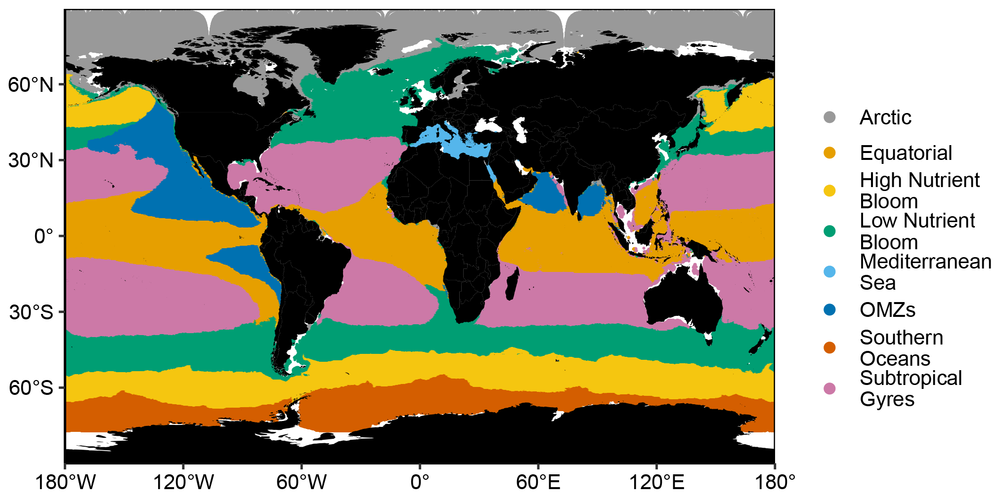
Figure 2Spatial distribution of the eight BGC regions obtained with a k-means clustering method applied to a data set of modeled climatological monthly time series of the 23 assessment metrics.
4.1 BGC regions of the global ocean
The k-means clustering algorithm identified eight distinct BGC regions (Fig. 2). Six of the eight BGC regions correspond to well-defined spatial regions and are, thus, named accordingly: “Arctic”, “equatorial” (Equ.), “Mediterranean Sea” (Med. Sea), “OMZs”, “subtropical gyres” (Sub. Gyres), and “Southern Oceans”. The other two BGC regions, i.e., “low nutrient bloom” (Low Nut. Bloom) and “high nutrient bloom” (High Nut. Bloom), are located in the North Atlantic and North Pacific oceans as well as in the lower latitudes of the Southern Oceans region. These two BGC regions correspond to ocean basins that experience a phytoplankton bloom in the springtime (Westberry et al., 2016). The main difference between these regions is that macronutrients such as nitrate and phosphate are abundant in one of them throughout the year due to phytoplankton growth being mainly limited by iron (Williams and Follows, 2011). Finally, it should be noted that outlier grid cells were not removed from the analysis; these outliers are mainly present in grid cells close to the coast. Additionally, grid cells with bathymetry shallower than 1000 m were not included in the clustering analysis, as metrics associated with mesopelagic processes cannot be calculated in these shallow grid cells.
The BGC regions found in our study are generally coherent with the biomes estimated in Fay and McKinley (2014) (hereinafter denoted FM2014). The Arctic and Southern Oceans regions correspond to the FM2014 ice biome. The Sub. Gyres region corresponds to the FM2014 subtropical permanently stratified biome. The Equ. BGC region represents a larger area than the equatorial biome in FM2014. The Low Nut. Bloom and High Nut. Bloom regions correspond to the FM2014 subtropical seasonally stratified and subpolar seasonally stratified biomes, respectively. These two BGC regions are coherent in the North Pacific and the Southern Oceans in both studies. They differ, however, in the North Atlantic: in FM2014, the subpolar North Atlantic is divided between the subtropical seasonally stratified and subpolar seasonally stratified biomes, whereas in our study this area is only represented by one BGC region – Low Nut. Bloom. Finally, the Med. Sea and OMZs BGC regions are not represented in FM2014. The main differences between our study and FM2014 are due to variations in the methodology used to identify BGC regions. In our study, we used 23 input variables to identify BGC regions, whereas clustering was based on only one BGC input variable (Chl a) and three physical variables (sea surface temperature, MLD, and sea-ice fraction) in FM2014. Our method allows the identification of specific BGC regions whose main characteristics are determined by variables other than Chl a, such as the OMZs BGC region. Furthermore, our method includes coastal areas and identifies the Med. Sea, which is not included in FM2014 because it is considered a coastal region, as a BGC region.
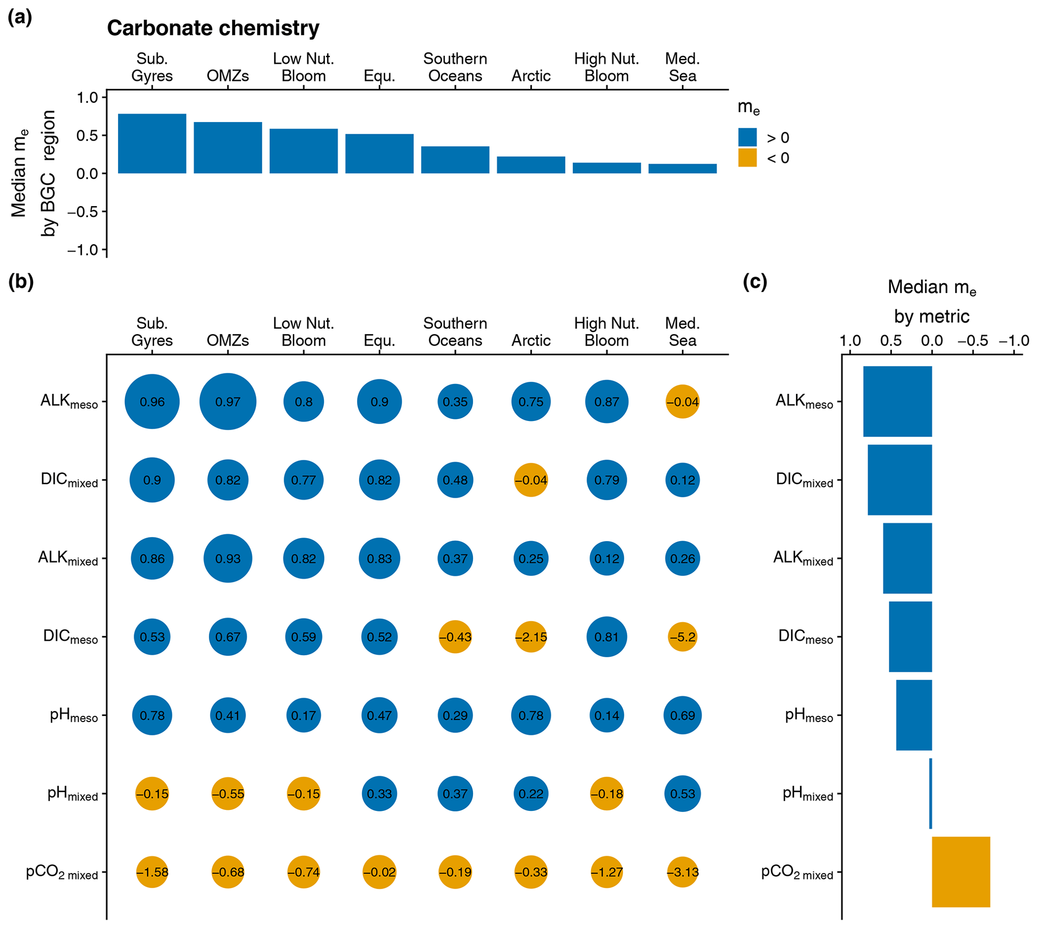
Figure 3(b) Bubble plot of the model efficiency statistical score (me) as a function of BGC regions (Arctic, equatorial (Equ.), high nutrient bloom (High Nut. Bloom), low nutrient bloom (Low Nut. Bloom), Mediterranean Sea (Med. Sea), oxygen minimum zones (OMZs), Southern Oceans, and subtropical gyres (Sub. Gyres)) and the assessment metrics associated with the carbonate chemistry (depth-averaged pCO2 in the mixed layer (pCO2 mixed), depth-averaged DIC in the mixed layer (DICmixed), depth-averaged Alk in the mixed layer (Alkmixed), depth-averaged DIC in the mesopelagic layer (DICmeso), depth-averaged Alk in the mesopelagic layer (Alkmeso), depth-averaged pH in the mixed layer (pHmixed), and depth-averaged pH in the mesopelagic layer (pHmeso)). The size of a bubble is proportional to the value of me. For a given assessment metric, the median values of me over all BGC regions are represented as a bar plot in panel (c). Similarly, for a given BGC region, the median values of me across all assessment metrics are represented as a bar plot in panel (a). In panel (b), the x and y axes are arranged in descending order of the median value of me over all assessment metrics and the median value of me over all BGC regions, respectively. The blue and orange colors correspond to a positive and negative me, respectively.
4.2 Model performance
Figures 3, 4, and 5 display the model efficiency (me) calculated for each assessment metric and BGC region. To enhance clarity, the me values are grouped by process, namely carbonate chemistry, biological carbon pump, and oxygen levels. The results are presented as bubble plots (Figs. 3b, 4b, 5b), where the size of the bubble is proportional to the me value. A bar plot (Figs. 3c, 4c, 5c) shows the median me value for a given assessment metric across all BGC regions, while another bar plot (Figs. 3a, 4a, 5a) shows the median me value for a given BGC region across all assessment metrics. Due to the limited number of assessment metrics associated with oxygen levels in most regions (i.e., 2), the mean is used instead of the median. The x and y axes in Figs. 3b, 4b, and 5b are arranged in descending order based on the median me value across all assessment metrics (as shown Figs. 3a, 4a, and 5a) and the median me value across all BGC regions (as shown in Figs. 3b, 4b, and 5b), respectively.
4.3 Carbonate chemistry
The model demonstrates improved performance with respect to predicting certain carbonate chemistry metrics (i.e., Alkmeso, DICmixed, Alkmixed, DICmeso, and pHmeso) compared with the BGC-Argo climatology, as indicated by median me values significantly greater than 0 (Fig. 3b, c). However, the model's ability to reproduce instantaneous variability in pHmixed is more limited, with a me value close to 0, indicating no improvement over a simple average of observed values. Furthermore, the model underperforms the BGC-Argo climatology for pCO2 mixed across all regions. Despite these limitations, the model provides an overall better estimate of carbonate chemistry dynamics in all BGC regions compared with the BGC-Argo climatology, as evidenced by Fig. 3a.
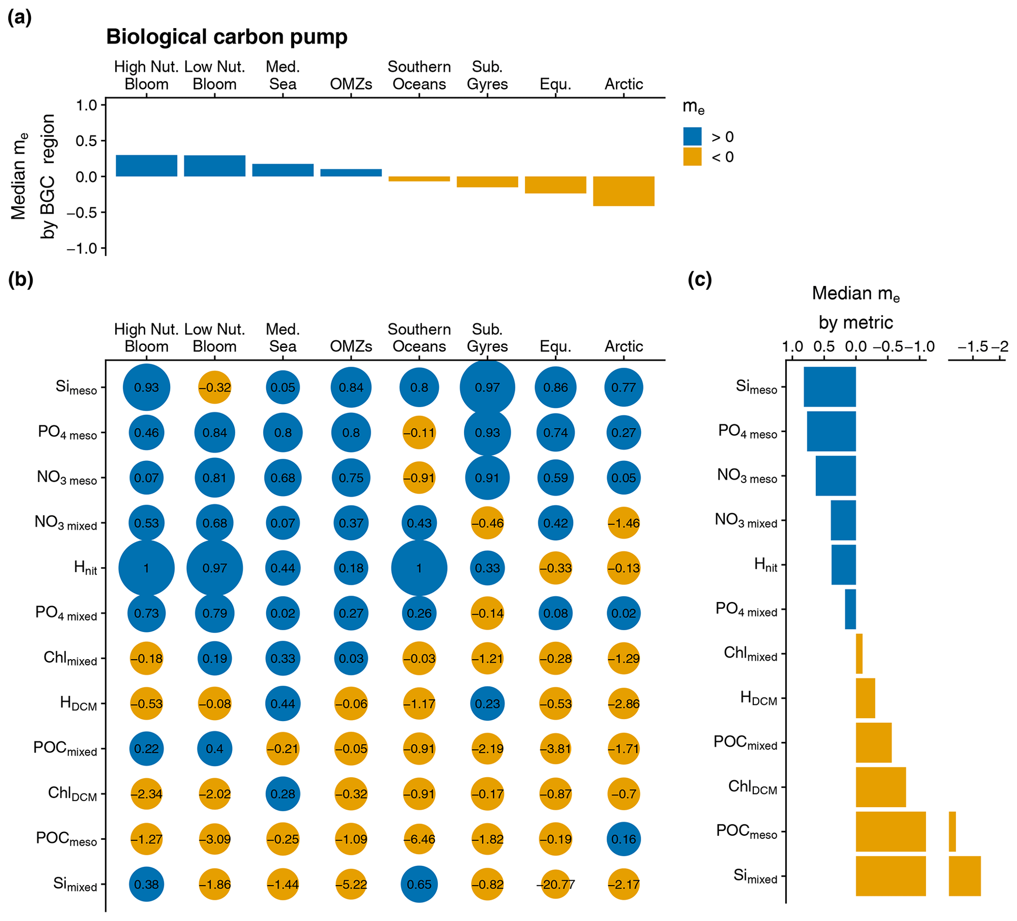
Figure 4Same as Fig. 3 but for the assessment metrics associated with the biological carbon pump: depth-averaged Chl a in the mixed layer (Chlmixed), depth-averaged NO3 in the mixed layer (NO3 mixed), depth-averaged PO4 in the mixed layer (PO4 mixed), depth-averaged Si in the mixed layer (Simixed), depth-averaged NO3 in the mesopelagic layer (NO3 meso), depth-averaged PO4 in the mesopelagic layer (PO4 meso), depth-averaged Si in the mesopelagic layer (Simeso), depth-averaged POC in the mixed layer (POCmixed), depth-averaged POC in the mesopelagic layer (POCmeso), magnitude of the DCM (ChlDCM), depth of the DCM (HDCM), and depth of the nitracline (Hnit).
4.4 Biological carbon pump
The efficiency of the model with respect to estimating the biological carbon pump metrics varies across both metrics and regions (Fig. 4a, b, c). The model outperforms the BGC-Argo climatology with respect to estimating PO4 and NO3 in the mesopelagic and mixed layer as well as with respect to estimating Simeso and Hnit. However, the model's ability to predict Si decreases significantly as one moves from the mesopelagic to the mixed layer. Additionally, the metrics associated with the first trophic level, such as Chlmixed, HDCM, ChlDCM, POCmixed, and POCmeso, are systematically outperformed by the BGC-Argo climatology, with median me values less than 0 in nearly all BGC regions (Fig. 4b). Regional analysis of the median me values (Fig. 4a) shows that the model performs better than the observational mean (median me values greater than 0) in only a few regions (i.e., High Nut. Bloom, Low Nut. Bloom, Med. Sea, and OMZs), indicating that the model performs relatively well in these regions but may not be as accurate in the other regions.
4.5 Oxygen levels
The model provides better estimates of mixed and mesopelagic O2 concentrations in most BGC regions compared with the BGC-Argo climatology, as evidenced by consistently positive me values in Fig. 5b. However, the BGC-Argo climatology provides a better representation of the magnitude of O2 min compared with the model, while the model performs better than the climatology with respect to predicting , although only in the OMZs BGC region. These results suggest that, while it performs well with respect to estimating mixed and mesopelagic O2 concentrations in most BGC regions, the model does not accurately capture the depth and magnitude of OMZs.
4.6 Discussion
The model outperforms the BGC-Argo climatology for DIC, Alk, NO3, and PO4 in the mesopelagic and mixed layers as well as for Si in the mesopelagic layer. We attribute this good performance to the effective application of climatological damping. As described in the Appendix, climatological damping mitigates the effects of physical data assimilation in the offline coupled hydrodynamic–biogeochemical system, which can lead to unrealistic drift of various biogeochemical variables. Specifically, we used the World Ocean Atlas 2013 (Garcia et al., 2013, 2014) for NO3, PO4, O2, and Si, whereas we utilized GLODAPv2 climatology (Lauvset et al., 2016) for DIC and Alk. However, our analysis revealed that the model's performance with respect to estimating Si in the mixed layer is significantly degraded compared with the mesopelagic layer, indicating the presence of additional factors affecting the model's ability to accurately estimate this variable. Further investigation is required to identify these factors and improve the model's performance with respect to estimating Si in the mixed layer.
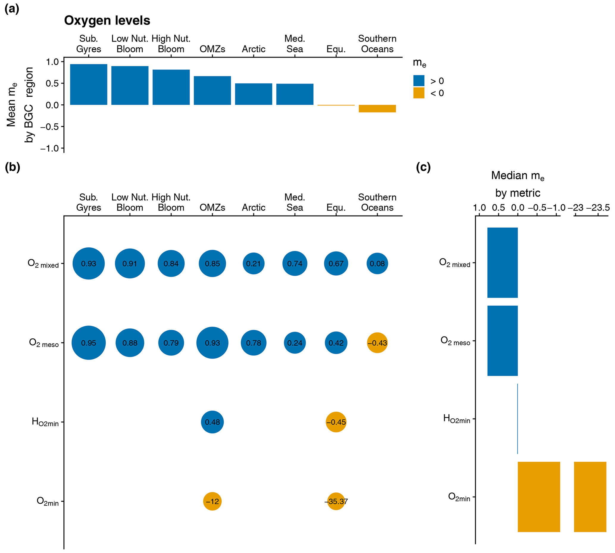
Figure 5Same as Fig. 3 but for the assessment metrics associated with the oxygen levels: depth-averaged O2 in the mixed layer (O2 mixed), depth-averaged O2 in the mesopelagic layer (O2 meso), value of the O2 minimum (O2 min), and depth of the O2 minimum (. Note that the bar plot in panel (a) represents the mean value of me over all assessment metrics.
For the three Chl a-related metrics, the model performs worse than the BGC-Argo climatology. This is unexpected, as the model incorporates a reduced-order Kalman filter (Lellouche et al., 2013) that assimilates daily L4 remotely sensed surface Chl a, providing a mixed-layer correction to the modeled Chl a (see Appendix). We verified that the assimilation of satellite Chl a improves the model's ability to predict Chl a, as the model–BGC-Argo-data misfit is lower compared with a simulation without assimilation (not shown). Furthermore, the model–satellite misfit was also found to be lower than the variability in the satellite data (European Union-Copernicus Marine Service, 2019). These results suggest that discrepancies between the assimilated satellite Chl a product and the BGC-Argo data may be responsible for the observed model–BGC-Argo-data misfit. Therefore, we suggest that future studies investigate the consistency between ocean color products and BGC-Argo Chl a products at a global scale, as these two products are expected to be assimilated together in future operational BGC systems (Ford, 2021).
Overall, the model also performs worse or no better than the BGC-Argo climatology with respect to predicting POC concentrations, the magnitude and depth of OMZs, pHmixed, and pCO2 mixed. The poor performance of PISCES-based simulations relative to BGC-Argo POC observations has been extensively studied in Gali et al. (2022). They pointed out that the large model–data misfit could be the result of an imperfect BGC-Argo POC–bbp conversion factor, unsuitable model parameters associated with POC dynamics, and missing processes in the model structure. Similarly, the poor model skill in capturing the OMZs' dynamics has also already been documented in several studies (Busecke et al., 2022; Schmidt et al., 2021; Cabré et al., 2015). All of these studies suggested that improving the ocean circulation in physical models may be the most important factor to improve the accuracy of OMZs' model predictions. Finally, the negative model efficiencies for pHmixed and pCO2 mixed can be attributed to the fact that these variables are driven by DIC, Alk, temperature, and salinity. Therefore, even small uncertainties in the model estimates of DIC, Alk (as shown in Fig. 3b), temperature, and salinity (Lellouche et al., 2018) can result in poor model performance in capturing the variability in pH and pCO2. This highlights the importance of accurately modeling these four variables to improve model estimates of pH and pCO2.
4.7 Recommendation for the design of the BGC-Argo observing system
Observing system simulation experiments (OSSEs) have been the primary tool used to provide information about the design of the BGC-Argo observing system (Ford, 2021; Biogeochemical-Argo Planning Group, 2016). OSSEs typically comprises a realistic “nature run”, which represents “the truth” from which synthetic observations are sampled. The synthetic observations represent the observing system to be designed. To test its impact on improving model's predictive skill, the synthetic observations are then assimilated in an “assimilative run”. The accuracy of the assimilative run is then evaluated against the nature run. Here, we use the real BGC-Argo observations to provide information about the design of the BGC-Argo network. More specifically, our aim is to gain information about the regions where the model errors are greater than the variability in the BGC-Argo data and, consequently, where BGC-Argo observations should be enhanced to improve the model accuracy via BGC-Argo data assimilation or process-oriented assessment studies.
For a given BGC region, we compute a single multivariate score corresponding to the median of the 23 me values associated with each assessment metric (Fig. 6). This is consistent with the fact that the BGC-Argo floats which are now deployed observe the five variables used to derive the assessment metrics, i.e., O2, Chla, NO3, bbp, and pH. In the Arctic and Southern Oceans BGC regions (typically north of 60∘ N and south of 60∘ S, respectively), the median me is barely greater than 0, suggesting that, in these regions, the model performs slightly better than a simple mean of the observed values. In these two regions, the model is not well constrained by the assimilation of remotely sensed Chl a because satellite observations of ocean color are not possible for most of the year due to ubiquitous cloud cover. In addition, the scarcity of in situ observations probably makes the climatological forcing less efficient in these regions. Together, these factors are likely to lead to poorer model performance compared with other regions. Consequently, we strongly recommend enhancing the Arctic region where BGC-Argo observations are scarce (Fig. 1) and where the winter–spring months are particularly undersampled (not shown). We also recommend maintaining the existing high density of BGC-Argo observations in the Southern Oceans. These observations are critical to better constrain the model in these two regions where the constraint of models via the assimilation of satellite observations is not possible for most of the year.
In this study, we propose a method based on the global data set of BGC-Argo observations, a k-means clustering algorithm, and 23 assessment metrics to simplify model–data comparison and provide information on the Copernicus Marine Service forecasting system predictive skill and the design of the BGC-Argo observing system. The k-means algorithm identified eight BGC regions in the model simulation that are consistent with the work of Fay and McKinley (2014). Within each BGC region and for each assessment metric, we compute a model efficiency statistical score that quantifies whether the model outperforms the BGC-Argo climatology by comparing the model–BGC-Argo-data mean-square difference with the observation variance.
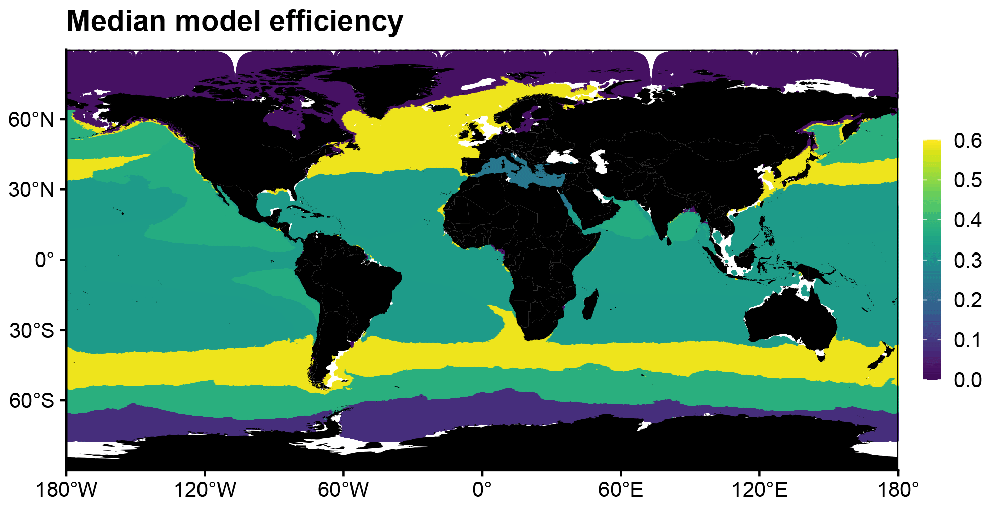
Figure 6Median of the 23 me values associated with each assessment metric by BGC region.
Overall, the model surpasses the BGC-Argo climatology with respect to predicting pH, DIC, Alk, O2, NO3, and PO4 in the mesopelagic and mixed layers as well as Si in the mesopelagic layer. For the other metrics, whose model predictions are outperformed by the BGC-Argo climatology, we provide suggestions to reduce the model–data misfit and, thus, increase the model efficiency. Regarding the estimation of Si in the mixed layer, we suggest the presence of additional factors that may affect the model's ability to accurately estimate this variable. Further investigation is necessary to identify these factors and improve the model's performance in this regard. For Chl a-related metrics, we recommend checking the consistency between ocean color products and BGC-Argo Chl a products at the global scale, as this may explain part of the misfit between the model, which assimilates satellite Chl a and BGC-Argo observations. The discrepancies between modeled and observed POC and OMZs have been already investigated in previous studies. It has been suggested that improving the BGC-Argo POC–bbp conversion factor, tuning the model parameters, and implementing missing processes in the model structure could decrease the model–data inconsistencies associated with POC dynamics. Similarly, improving the ocean circulation in physical models should improve the accuracy of OMZ model predictions. Finally, pHmixed and pCO2 mixed should be better modeled if the uncertainties associated with DIC, Alk, temperature, and salinity in the mixed layer are reduced.
The proposed method can also be used to optimize the design of the BGC-Argo network. In particular, the regions where BGC-Argo observations should be enhanced to reduce the model–data misfit via the assimilation of BGC-Argo data or process-oriented assessment studies. We strongly recommend enhancing the observation density in the Arctic region and maintaining the existing high density of observations in the Southern Oceans. These are two regions where the model error is barely less than the variability in BGC-Argo observations and where it is not possible to use satellite observations to constrain the models via assimilation most of the year.
The model used in this study features the offline coupled NEMO–PISCES model with a horizontal resolution, 50 vertical levels (22 levels in the upper 100 m, and the vertical resolution decreases from 1 m near the surface to 450 m near the ocean bottom), and a daily temporal resolution, covering the period from 2009 to 2020.
The biogeochemical model PISCES v2 (Aumont et al., 2015) is a model of intermediate complexity designed for global ocean applications and is part of NEMO modeling platform. It features 24 prognostic variables and includes five nutrients that limit phytoplankton growth (nitrate, ammonium, phosphate, silicate, and iron) and four living compartments (two phytoplankton size classes, nanophytoplankton and diatoms, which are small and large, respectively, and two zooplankton size classes, microzooplankton and mesozooplankton, which are small and large, respectively); the bacterial pool is not explicitly modeled. PISCES distinguishes three nonliving detrital pools for organic carbon, particles of calcium carbonate, and biogenic silicate. Additionally, the model simulates the carbonate system and dissolved oxygen. PISCES has been successfully used in a variety of biogeochemical studies, both at the regional and global scale (Bopp et al., 2005; Gehlen et al., 2006, 2007; Gutknecht et al., 2019; Lefèvre et al., 2019; Schneider et al., 2008; Séférian et al., 2013; Steinacher et al., 2010; Tagliabue et al., 2010).
The dynamical component is the latest Mercator Ocean global high-resolution ocean model system, extensively described and validated in Lellouche et al. (2013, 2018). This system provides daily and coarsened fields of horizontal and vertical current velocities, vertical eddy diffusivity, mixed-layer depth, sea-ice fraction, potential temperature, salinity, sea surface height, surface wind speed, freshwater fluxes, and net surface solar shortwave irradiance that drive the transport of biogeochemical tracers. This system also features a reduced-order Kalman filter based on the singular evolutive extended Kalman filter (SEEK) formulation introduced by Pham et al. (1998), which assimilates, on a 7 d assimilation cycle, along-track altimeter data, satellite sea surface temperature and sea-ice concentration from Operational Sea Surface Temperature and Sea Ice Analysis (OSTIA), and in situ temperature and salinity vertical profiles from the Coriolis Dataset for ReAnalysis (CORA) version 4.2 in situ database.
In addition, the biogeochemical component of the coupled system also embeds a reduced-order Kalman filter (similar to the abovementioned filter) that operationally assimilates daily L4 remotely sensed surface chlorophyll (European Union-Copernicus Marine Service, 2022). Thanks to a multivariate formulation of model error covariances, the system is able to provide a three-dimensional correction to the nanophytoplankton, diatoms, and nitrates model concentrations from the surface chlorophyll data provided by satellite observations.
In parallel, climatological damping is applied to nitrate, phosphate, oxygen, and silicate with the World Ocean Atlas 2013, to dissolved inorganic carbon and alkalinity with the GLODAPv2 climatology (Lauvset et al., 2016), and to dissolved organic carbon and iron with a 4000-year PISCES climatological run. This relaxation is set to mitigate the impact of the physical data assimilation in the offline coupled hydrodynamic–biogeochemical system, leading to significant rises in nutrients in the equatorial belt area and resulting in an unrealistic drift of various biogeochemical variables, such as chlorophyll, nitrate, and phosphate (Fennel et al., 2019; Park et al., 2018). The timescale associated with this climatological damping is set to 1 year and allows a smooth constraint that has been shown to be efficient to reduce the model drift.
The Global Ocean Biogeochemistry Analysis and Forecast system data are publicly available for download via the Copernicus Marine Service (https://doi.org/10.48670/MOI-00015, European Union-Copernicus Marine Service, 2019). Data prior to 4 May 2019 must be requested directly from the authors. The BGC-Argo data and metadata were collected and made freely available by the international Argo program and the national programs that contribute to it (https://doi.org/10.17882/42182, Argo, 2023). The Argo program is part of the Global Ocean Observing System (ftp://ftp.ifremer.fr/ifremer/argo, last access: January 2023).
AM, GC, FD, SS, and VT conceived of the study. AM, HC, FD, RS, and VT designed the study. AM and RS process the BGC-Argo float data. AM analyzed the data. AM wrote the first draft of the manuscript. HC, GC, FD, EG, PL, CP, SS, RS, VT, and AT contributed to the subsequent drafts. All authors read and approved the final draft.
The contact author has declared that none of the authors has any competing interests.
Publisher’s note: Copernicus Publications remains neutral with regard to jurisdictional claims in published maps and institutional affiliations.
This article is part of the special issue “Biogeochemistry in the BGC-Argo era: from process studies to ecosystem forecasts (BG/OS inter-journal SI)”. It is not associated with a conference.
The authors would like to thank the International Argo Program, the Coriolis Project and the Copernicus Marine Service (CMEMS) for their contribution in making the data publicly and freely available, which allowed the successful completion of this study. Part of this work was carried out as part of the BIOOPTIMOD and MASSIMILI CMEMS Service Evolution projects, and we gratefully acknowledge their support.
This project has been funded by the European Union's Horizon 2020 Research and Innovation program under grant agreement no. 862626 (EuroSea). This paper is a contribution to the following research projects: NAOS (funded by the Agence Nationale de la Recherche under the French “Equipement d'avenir” program, grant no. ANR J11R107-F), remOcean (funded by the European Research Council, grant no. 246777), and the French Bio-Argo program (BGC-Argo France, funded by CNES-TOSCA, LEFE-GMMC).
This paper was edited by Tina Treude and reviewed by Marcello Vichi and two anonymous referees.
Allen, J. I., Somerfield, P. J., and Gilbert, F. J.: Quantifying uncertainty in high-resolution coupled hydrodynamic-ecosystem models, J. Mar. Syst., 64, 3–14, https://doi.org/10.1016/j.jmarsys.2006.02.010, 2007.
Álvarez, E., Lazzari, P., and Cossarini, G.: Phytoplankton diversity emerging from chromatic adaptation and competition for light, Prog. Oceanogr., 204, 102789, https://doi.org/10.1016/j.pocean.2022.102789, 2022.
Argo: Argo Float Data and Metadata from Global Data Assembly Centre (Argo GDAC), SEANOE [data set], https://doi.org/10.17882/42182, 2023.
Aumont, O., Ethé, C., Tagliabue, A., Bopp, L., and Gehlen, M.: PISCES-v2: an ocean biogeochemical model for carbon and ecosystem studies, Geosci. Model Dev., 8, 2465–2513, https://doi.org/10.5194/gmd-8-2465-2015, 2015.
Barbieux, M., Uitz, J., Gentili, B., Pasqueron de Fommervault, O., Mignot, A., Poteau, A., Schmechtig, C., Taillandier, V., Leymarie, E., Penkerc'h, C., D'Ortenzio, F., Claustre, H., and Bricaud, A.: Bio-optical characterization of subsurface chlorophyll maxima in the Mediterranean Sea from a Biogeochemical-Argo float database, Biogeosciences, 16, 1321–1342, https://doi.org/10.5194/bg-16-1321-2019, 2019.
Biogeochemical-Argo Planning Group: The scientific rationale, design and implementation plan for a Biogeochemical-Argo float array, https://doi.org/10.13155/46601, 2016.
Bittig, H. C., Steinhoff, T., Claustre, H., Fiedler, B., Williams, N. L., Sauzède, R., Körtzinger, A., and Gattuso, J.-P.: An alternative to static climatologies: robust estimation of open ocean CO2 variables and nutrient concentrations from T, S, and O2 data using Bayesian neural networks, Front. Mar. Sci., 5, 328, https://doi.org/10.3389/fmars.2018.00328, 2018.
Bittig, H. C., Maurer, T. L., Plant, J. N., Wong, A. P., Schmechtig, C., Claustre, H., Trull, T. W., Udaya Bhaskar, T. V. S., Boss, E., and Dall'Olmo, G.: A BGC-Argo guide: Planning, deployment, data handling and usage, Front. Mar. Sci., 6, 502, https://doi.org/10.3389/fmars.2019.00502, 2019.
Bock, N., Cornec, M., Claustre, H., and Duhamel, S.: Biogeographical Classification of the Global Ocean From BGC-Argo Floats, Global Biogeochem. Cy., 36, https://doi.org/10.1029/2021GB007233, 2022.
Bojinski, S., Verstraete, M., Peterson, T. C., Richter, C., Simmons, A., and Zemp, M.: The concept of essential climate variables in support of climate research, applications, and policy, B. Am. Meteorol. Soc., 95, 1431–1443, 2014.
Bopp, L., Aumont, O., Cadule, P., Alvain, S., and Gehlen, M.: Response of diatoms distribution to global warming and potential implications: A global model study, Geophys. Res. Lett., 32, https://doi.org/10.1029/2005GL023653, 2005.
Boyer, T. P., Antonov, J. I., Baranova, O. K., Garcia, H. E., Johnson, D. R., Mishonov, A. V., O'Brien, T. D., Seidov, D., Smolyar, I., and Zweng, M. M.: World Ocean Database 2013, Silver Spring, MD, National Oceanographic Data Center, 208 pp., (NOAA Atlas NESDIS, 72), https://doi.org/10.25607/OBP-1454, 2013.
Breitburg, D., Levin, L. A., Oschlies, A., Grégoire, M., Chavez, F. P., Conley, D. J., Garçon, V., Gilbert, D., Gutiérrez, D., Isensee, K., Jacinto, G. S., Limburg, K. E., Montes, I., Naqvi, S. W. A., Pitcher, G. C., Rabalais, N. N., Roman, M. R., Rose, K. A., Seibel, B. A., Telszewski, M., Yasuhara, M., and Zhang, J.: Declining oxygen in the global ocean and coastal waters, Science, 359, 6371, https://doi.org/10.1126/science.aam7240, 2018.
Briggs, N., Perry, M. J., Cetinić, I., Lee, C., D'Asaro, E., Gray, A. M., and Rehm, E.: High-resolution observations of aggregate flux during a sub-polar North Atlantic spring bloom, Deep-Sea Res. Pt. I, 58, 1031–1039, https://doi.org/10.1016/j.dsr.2011.07.007, 2011.
Busecke, J. J. M., Resplandy, L., Ditkovsky, S. J., and John, J. G.: Diverging Fates of the Pacific Ocean Oxygen Minimum Zone and Its Core in a Warming World, AGU Adv., 3, e2021AV000470, https://doi.org/10.1029/2021AV000470, 2022.
Cabré, A., Marinov, I., Bernardello, R., and Bianchi, D.: Oxygen minimum zones in the tropical Pacific across CMIP5 models: mean state differences and climate change trends, Biogeosciences, 12, 5429–5454, https://doi.org/10.5194/bg-12-5429-2015, 2015.
Capuzzo, E., Lynam, C. P., Barry, J., Stephens, D., Forster, R. M., Greenwood, N., McQuatters-Gollop, A., Silva, T., van Leeuwen, S. M., and Engelhard, G. H.: A decline in primary production in the North Sea over 25 years, associated with reductions in zooplankton abundance and fish stock recruitment, Glob. Change Biol., 24, 352–364, https://doi.org/10.1111/gcb.13916, 2018.
Cermeno, P., Dutkiewicz, S., Harris, R. P., Follows, M., Schofield, O., and Falkowski, P. G.: The role of nutricline depth in regulating the ocean carbon cycle, P. Natl. Acad. Sci. USA, 105, 20344–20349, https://doi.org/10.1073/pnas.0811302106, 2008.
Claustre, H., Johnson, K. S., and Takeshita, Y.: Observing the Global Ocean with Biogeochemical-Argo, Annu. Rev. Mar. Sci., 12, 23–48, https://doi.org/10.1146/annurev-marine-010419-010956, 2020.
Crowder, L. B., Hazen, E. L., Avissar, N., Bjorkland, R., Latanich, C., and Ogburn, M. B.: The Impacts of Fisheries on Marine Ecosystems and the Transition to Ecosystem-Based Management, Annu. Rev. Ecol. Evol. Syst., 39, 259–278, https://doi.org/10.1146/annurev.ecolsys.39.110707.173406, 2008.
Cullen, J. J.: Subsurface Chlorophyll Maximum Layers: Enduring Enigma or Mystery Solved?, Annu. Rev. Mar. Sci., 7, 207–239, https://doi.org/10.1146/annurev-marine-010213-135111, 2015.
Doney, S. C., Lima, I., Moore, J. K., Lindsay, K., Behrenfeld, M. J., Westberry, T. K., Mahowald, N., Glover, D. M., and Takahashi, T.: Skill metrics for confronting global upper ocean ecosystem-biogeochemistry models against field and remote sensing data, J. Mar. Syst., 76, 95–112, https://doi.org/10.1016/j.jmarsys.2008.05.015, 2009.
D'Ortenzio, F. and Ribera d'Alcalà, M.: On the trophic regimes of the Mediterranean Sea: a satellite analysis, Biogeosciences, 6, 139–148, https://doi.org/10.5194/bg-6-139-2009, 2009.
D'Ortenzio, F., Taillandier, V., Claustre, H., Prieur, L. M., Leymarie, E., Mignot, A., Poteau, A., Penkerc'h, C., and Schmechtig, C. M.: Biogeochemical Argo: The Test Case of the NAOS Mediterranean Array, Front. Mar. Sci., 7, p. 120, https://doi.org/10.3389/fmars.2020.00120, 2020.
Dutkiewicz, S., Hickman, A. E., Jahn, O., Gregg, W. W., Mouw, C. B., and Follows, M. J.: Capturing optically important constituents and properties in a marine biogeochemical and ecosystem model, Biogeosciences, 12, 4447–4481, https://doi.org/10.5194/bg-12-4447-2015, 2015.
Eriksen, M., Lebreton, L. C. M., Carson, H. S., Thiel, M., Moore, C. J., Borerro, J. C., Galgani, F., Ryan, P. G., and Reisser, J.: Plastic Pollution in the World's Oceans: More than 5 Trillion Plastic Pieces Weighing over 250,000 Tons Afloat at Sea, PLoS ONE, 9, e111913, https://doi.org/10.1371/journal.pone.0111913, 2014.
European Union-Copernicus Marine Service: Global Ocean-In-Situ Near-Real-Time Observations, https://doi.org/10.48670/MOI-00036, 2015.
European Union-Copernicus Marine Service: Global Ocean Biogeochemistry Analysis and Forecast, Mercator Ocean International [data set], https://doi.org/10.48670/MOI-00015, 2019.
European Union-Copernicus Marine Service: Global Ocean 3D chlorophyll-a concentration, Particulate Backscattering coefficient and Particulate Organic Carbon, https://doi.org/10.48670/MOI-00046, 2020.
European Union-Copernicus Marine Service: Global Ocean Colour (Copernicus-GlobColour), Bio-Geo-Chemical, L4 (monthly and interpolated) from Satellite Observations (Near Real Time), https://doi.org/10.48670/MOI-00279, 2022.
Fay, A. R. and McKinley, G. A.: Global open-ocean biomes: mean and temporal variability, Earth Syst. Sci. Data, 6, 273–284, https://doi.org/10.5194/essd-6-273-2014, 2014.
Fennel, K., Gehlen, M., Brasseur, P., Brown, C. W., Ciavatta, S., Cossarini, G., Crise, A., Edwards, C. A., Ford, D., Friedrichs, M. A. M., Gregoire, M., Jones, E., Kim, H.-C., Lamouroux, J., Murtugudde, R., Perruche, C., and the GODAE OceanView Marine Ecosystem Analysis and Prediction Task Team: Advancing Marine Biogeochemical and Ecosystem Reanalyses and Forecasts as Tools for Monitoring and Managing Ecosystem Health, Front. Mar. Sci., 6, 89, https://doi.org/10.3389/fmars.2019.00089, 2019.
Fennel, K., Mattern, J. P., Doney, S. C., Bopp, L., Moore, A. M., Wang, B., and Yu, L.: Ocean biogeochemical modelling, Nat. Rev. Methods Primer, 2, 1–21, https://doi.org/10.1038/s43586-022-00154-2, 2022.
Ford, D.: Assimilating synthetic Biogeochemical-Argo and ocean colour observations into a global ocean model to inform observing system design, Biogeosciences, 18, 509–534, https://doi.org/10.5194/bg-18-509-2021, 2021.
Friedlingstein, P., O'Sullivan, M., Jones, M. W., Andrew, R. M., Gregor, L., Hauck, J., Le Quéré, C., Luijkx, I. T., Olsen, A., Peters, G. P., Peters, W., Pongratz, J., Schwingshackl, C., Sitch, S., Canadell, J. G., Ciais, P., Jackson, R. B., Alin, S. R., Alkama, R., Arneth, A., Arora, V. K., Bates, N. R., Becker, M., Bellouin, N., Bittig, H. C., Bopp, L., Chevallier, F., Chini, L. P., Cronin, M., Evans, W., Falk, S., Feely, R. A., Gasser, T., Gehlen, M., Gkritzalis, T., Gloege, L., Grassi, G., Gruber, N., Gürses, Ö., Harris, I., Hefner, M., Houghton, R. A., Hurtt, G. C., Iida, Y., Ilyina, T., Jain, A. K., Jersild, A., Kadono, K., Kato, E., Kennedy, D., Klein Goldewijk, K., Knauer, J., Korsbakken, J. I., Landschützer, P., Lefèvre, N., Lindsay, K., Liu, J., Liu, Z., Marland, G., Mayot, N., McGrath, M. J., Metzl, N., Monacci, N. M., Munro, D. R., Nakaoka, S.-I., Niwa, Y., O'Brien, K., Ono, T., Palmer, P. I., Pan, N., Pierrot, D., Pocock, K., Poulter, B., Resplandy, L., Robertson, E., Rödenbeck, C., Rodriguez, C., Rosan, T. M., Schwinger, J., Séférian, R., Shutler, J. D., Skjelvan, I., Steinhoff, T., Sun, Q., Sutton, A. J., Sweeney, C., Takao, S., Tanhua, T., Tans, P. P., Tian, X., Tian, H., Tilbrook, B., Tsujino, H., Tubiello, F., van der Werf, G. R., Walker, A. P., Wanninkhof, R., Whitehead, C., Willstrand Wranne, A., Wright, R., Yuan, W., Yue, C., Yue, X., Zaehle, S., Zeng, J., and Zheng, B.: Global Carbon Budget 2022, Earth Syst. Sci. Data, 14, 4811–4900, https://doi.org/10.5194/essd-14-4811-2022, 2022.
Galí, M., Falls, M., Claustre, H., Aumont, O., and Bernardello, R.: Bridging the gaps between particulate backscattering measurements and modeled particulate organic carbon in the ocean, Biogeosciences, 19, 1245–1275, https://doi.org/10.5194/bg-19-1245-2022, 2022.
Garcia, H. E., Locarnini, R. A., Boyer, T. P., Antonov, J. I., Baranova, O. K., Zweng, M. M., Reagan, J. R., Johnson, D. R., Mishonov, A. V., and Levitus, S.: World ocean atlas 2013, Volume 4, Dissolved inorganic nutrients (phosphate, nitrate, silicate), https://doi.org/10.7289/V5J67DWD, 2013.
Garcia, H. E., Boyer, T. P., Locarnini, R. A., Antonov, J. I., Mishonov, A. V., Baranova, O. K., Zweng, M. M., Reagan, J. R., Johnson, D. R., and Levitus, S.: World ocean atlas 2013. Volume 3, Dissolved oxygen, apparent oxygen utilization, and oxygen saturation, https://doi.org/10.7289/V5XG9P2W, 2014.
Gasparin, F., Cravatte, S., Greiner, E., Perruche, C., Hamon, M., Van Gennip, S., and Lellouche, J.-M.: Excessive productivity and heat content in tropical Pacific analyses: Disentangling the effects of in situ and altimetry assimilation, Ocean Model., 160, 101768, https://doi.org/10.1016/j.ocemod.2021.101768, 2021.
Gehlen, M., Bopp, L., Emprin, N., Aumont, O., Heinze, C., and Ragueneau, O.: Reconciling surface ocean productivity, export fluxes and sediment composition in a global biogeochemical ocean model, Biogeosciences, 3, 521–537, https://doi.org/10.5194/bg-3-521-2006, 2006.
Gehlen, M., Gangstø, R., Schneider, B., Bopp, L., Aumont, O., and Ethe, C.: The fate of pelagic CaCO3 production in a high CO2 ocean: a model study, Biogeosciences, 4, 505–519, https://doi.org/10.5194/bg-4-505-2007, 2007.
Gutknecht, E., Reffray, G., Mignot, A., Dabrowski, T., and Sotillo, M. G.: Modelling the marine ecosystem of Iberia–Biscay–Ireland (IBI) European waters for CMEMS operational applications, Ocean Sci., 15, 1489–1516, https://doi.org/10.5194/os-15-1489-2019, 2019.
Hartigan, J. A. and Wong, M. A.: Algorithm AS 136: A k-means Clustering Algorithm, Appl. Stat., 28, 100, https://doi.org/10.2307/2346830, 1979.
Hipsey, M. R., Gal, G., Arhonditsis, G. B., Carey, C. C., Elliott, J. A., Frassl, M. A., Janse, J. H., de Mora, L., and Robson, B. J.: A system of metrics for the assessment and improvement of aquatic ecosystem models, Environ. Model. Softw., 128, 104697, https://doi.org/10.1016/j.envsoft.2020.104697, 2020.
Iida, Y., Takatani, Y., Kojima, A., and Ishii, M.: Global trends of ocean CO 2 sink and ocean acidification: an observation-based reconstruction of surface ocean inorganic carbon variables, J. Oceanogr., 77, 323–358, 2020.
Johnson, Plant, J. N., Coletti, L. J., Jannasch, H. W., Sakamoto, C. M., Riser, S. C., Swift, D. D., Williams, N. L., Boss, E., Haëntjens, N., Talley, L. D., and Sarmiento, J. L.: Biogeochemical sensor performance in the SOCCOM profiling float array: Soccom biogeochemical sensor performance, J. Geophys. Res.-Oceans, 122, 6416–6436, https://doi.org/10.1002/2017JC012838, 2017.
Johnson, Plant, J. N. and Maurer, T. L.: Processing BGC-Argo pH data at the DAC level, Argo data management, https://doi.org/10.13155/57195, 2018a.
Johnson, Pasqueron De Fommervault, O., Serra, R., D'Ortenzio, F., Schmechtig, C., Claustre, H., and Poteau, A.: Processing Bio-Argo nitrate concentration at the DAC Level, Version 1.1, March 3rd 2018, IFREMER for Argo Data Management, 22 pp., https://doi.org/10.13155/46121, 2018b.
Kheireddine, M., Mayot, N., Ouhssain, M., and Jones, B. H.: Regionalization of the Red Sea Based on Phytoplankton Phenology: A Satellite Analysis, J. Geophys. Res.-Oceans, 126, https://doi.org/10.1029/2021JC017486, 2021.
Lacour, L., Claustre, H., Prieur, L., and D'Ortenzio, F.: Phytoplankton biomass cycles in the North Atlantic subpolar gyre: A similar mechanism for two different blooms in the Labrador Sea: The labrador sea blooms, Geophys. Res. Lett., 42, 5403–5410, https://doi.org/10.1002/2015GL064540, 2015.
Lavigne, H., D'Ortenzio, F., Migon, C., Claustre, H., Testor, P., d'Alcalà, M. R., Lavezza, R., Houpert, L., and Prieur, L.: Enhancing the comprehension of mixed layer depth control on the Mediterranean phytoplankton phenology: Mediterranean Phytoplankton Phenology, J. Geophys. Res.-Oceans, 118, 3416–3430, https://doi.org/10.1002/jgrc.20251, 2013.
Lauvset, S. K., Key, R. M., Olsen, A., van Heuven, S., Velo, A., Lin, X., Schirnick, C., Kozyr, A., Tanhua, T., Hoppema, M., Jutterström, S., Steinfeldt, R., Jeansson, E., Ishii, M., Pérez, F. F., Suzuki, T., and Watelet, S.: A new global interior ocean mapped climatology: the GLODAP version 2, Earth Syst. Sci. Data, 8, 325–340, https://doi.org/10.5194/essd-8-325-2016, 2016.
Lazzari, P., Solidoro, C., Ibello, V., Salon, S., Teruzzi, A., Béranger, K., Colella, S., and Crise, A.: Seasonal and inter-annual variability of plankton chlorophyll and primary production in the Mediterranean Sea: a modelling approach, Biogeosciences, 9, 217–233, https://doi.org/10.5194/bg-9-217-2012, 2012.
Lazzari, P., Solidoro, C., Salon, S., and Bolzon, G.: Spatial variability of phosphate and nitrate in the Mediterranean Sea: A modeling approach, Deep Sea Res., 108, 39–52, https://doi.org/10.1016/j.dsr.2015.12.006, 2016.
Lefèvre, N., Veleda, D., Tyaquiçã, P., Perruche, C., Diverrès, D., and Ibánhez, J. S. P.: Basin-Scale Estimate of the Sea-Air CO2 Flux During the 2010 Warm Event in the Tropical North Atlantic, J. Geophys. Res.-Biogeo., 124, 973–986, https://doi.org/10.1029/2018JG004840, 2019.
Lellouche, J.-M., Greiner, E., Le Galloudec, O., Garric, G., Regnier, C., Drevillon, M., Benkiran, M., Testut, C.-E., Bourdalle-Badie, R., Gasparin, F., Hernandez, O., Levier, B., Drillet, Y., Remy, E., and Le Traon, P.-Y.: Recent updates to the Copernicus Marine Service global ocean monitoring and forecasting real-time high-resolution system, Ocean Sci., 14, 1093–1126, https://doi.org/10.5194/os-14-1093-2018, 2018.
Lellouche, J.-M., Le Galloudec, O., Drévillon, M., Régnier, C., Greiner, E., Garric, G., Ferry, N., Desportes, C., Testut, C.-E., Bricaud, C., Bourdallé-Badie, R., Tranchant, B., Benkiran, M., Drillet, Y., Daudin, A., and De Nicola, C.: Evaluation of global monitoring and forecasting systems at Mercator Océan, Ocean Sci., 9, 57–81, https://doi.org/10.5194/os-9-57-2013, 2013.
Letelier, R. M., Karl, D. M., Abbott, M. R., and Bidigare, R. R.: Light driven seasonal patterns of chlorophyll and nitrate in the lower euphotic zone of the North Pacific Subtropical Gyre, Limnol. Oceanogr., 49, 508–519, 2004.
Lynch, D. R., McGillicuddy, D. J., and Werner, F. E.: Skill assessment for coupled biological/physical models of marine systems, J. Mar. Syst., 1, 1–3, 2009.
Macías, D., Stips, A., and Garcia-Gorriz, E.: The relevance of deep chlorophyll maximum in the open Mediterranean Sea evaluated through 3D hydrodynamic-biogeochemical coupled simulations, Ecol. Model., 281, 26–37, 2014.
Mayot, N., D'Ortenzio, F., Ribera d'Alcalà, M., Lavigne, H., and Claustre, H.: Interannual variability of the Mediterranean trophic regimes from ocean color satellites, Biogeosciences, 13, 1901–1917, https://doi.org/10.5194/bg-13-1901-2016, 2016.
Mignot, A., Claustre, H., Uitz, J., Poteau, A., D'Ortenzio, F., and Xing, X.: Understanding the seasonal dynamics of phytoplankton biomass and the deep chlorophyll maximum in oligotrophic environments: A Bio-Argo float investigation, GGlobal Biogeochem. Cy., 28, 856–876, https://doi.org/10.1002/2013GB004781, 2014.
Mignot, A., Claustre, H., D'Ortenzio, F., Xing, X., Poteau, A., and Ras, J.: From the shape of the vertical profile of in vivo fluorescence to Chlorophyll-a concentration, Biogeosciences, 8, 2391–2406, https://doi.org/10.5194/bg-8-2391-2011, 2011.
Mignot, A., D'Ortenzio, F., Taillandier, V., Cossarini, G., and Salon, S.: Quantifying Observational Errors in Biogeochemical-Argo Oxygen, Nitrate, and Chlorophyll a Concentrations, Geophys. Res. Lett., 46, 4330–4337, https://doi.org/10.1029/2018GL080541, 2019.
Olsen, A., Key, R. M., van Heuven, S., Lauvset, S. K., Velo, A., Lin, X., Schirnick, C., Kozyr, A., Tanhua, T., Hoppema, M., Jutterström, S., Steinfeldt, R., Jeansson, E., Ishii, M., Pérez, F. F., and Suzuki, T.: The Global Ocean Data Analysis Project version 2 (GLODAPv2) – an internally consistent data product for the world ocean, Earth Syst. Sci. Data, 8, 297–323, https://doi.org/10.5194/essd-8-297-2016, 2016.
Omand, M. M. and Mahadevan, A.: The shape of the oceanic nitracline, Biogeosciences, 12, 3273–3287, https://doi.org/10.5194/bg-12-3273-2015, 2015.
Osman, M. B., Das, S. B., Trusel, L. D., Evans, M. J., Fischer, H., Grieman, M. M., Kipfstuhl, S., McConnell, J. R., and Saltzman, E. S.: Industrial-era decline in subarctic Atlantic productivity, Nature, 569, 551–555, https://doi.org/10.1038/s41586-019-1181-8, 2019.
Park, J.-Y., Stock, C. A., Yang, X., Dunne, J. P., Rosati, A., John, J., and Zhang, S.: Modeling Global Ocean Biogeochemistry With Physical Data Assimilation: A Pragmatic Solution to the Equatorial Instability, J. Adv. Model. Earth Syst., 10, 891–906, https://doi.org/10.1002/2017MS001223, 2018.
Paulmier, A. and Ruiz-Pino, D.: Oxygen minimum zones (OMZs) in the modern ocean, Prog. Oceanogr., 80, 113–128, 2009.
Richardson, K. and Bendtsen, J.: Vertical distribution of phytoplankton and primary production in relation to nutricline depth in the open ocean, Mar. Ecol. Prog. Ser., 620, 33–46, https://doi.org/10.3354/meps12960, 2019.
Rousseeuw, P. J.: Silhouettes: A graphical aid to the interpretation and validation of cluster analysis, J. Comput. Appl. Math., 20, 53–65, https://doi.org/10.1016/0377-0427(87)90125-7, 1987.
Roxy, M. K., Modi, A., Murtugudde, R., Valsala, V., Panickal, S., Prasanna Kumar, S., Ravichandran, M., Vichi, M., and Lévy, M.: A reduction in marine primary productivity driven by rapid warming over the tropical Indian Ocean, Geophys. Res. Lett., 43, 826–833, https://doi.org/10.1002/2015GL066979, 2016.
Russell, J. L., Kamenkovich, I., Bitz, C., Ferrari, R., Gille, S. T., Goodman, P. J., Hallberg, R., Johnson, K., Khazmutdinova, K., and Marinov, I.: Metrics for the evaluation of the Southern Ocean in coupled climate models and earth system models, J. Geophys. Res.-Oceans, 123, 3120–3143, 2018.
Salon, S., Cossarini, G., Bolzon, G., Feudale, L., Lazzari, P., Teruzzi, A., Solidoro, C., and Crise, A.: Novel metrics based on Biogeochemical Argo data to improve the model uncertainty evaluation of the CMEMS Mediterranean marine ecosystem forecasts, Ocean Sci., 15, 997–1022, https://doi.org/10.5194/os-15-997-2019, 2019.
Sauzède, R., Bittig, H. C., Claustre, H., Pasqueron de Fommervault, O., Gattuso, J.-P., Legendre, L., and Johnson, K. S.: Estimates of Water-Column Nutrient Concentrations and Carbonate System Parameters in the Global Ocean: A Novel Approach Based on Neural Networks, Front. Mar. Sci., 4, p. 128, https://doi.org/10.3389/fmars.2017.00128, 2017.
Schartau, M., Wallhead, P., Hemmings, J., Löptien, U., Kriest, I., Krishna, S., Ward, B. A., Slawig, T., and Oschlies, A.: Reviews and syntheses: parameter identification in marine planktonic ecosystem modelling, Biogeosciences, 14, 1647–1701, https://doi.org/10.5194/bg-14-1647-2017, 2017.
Schmechtig, C., Poteau, A., Claustre, H., D'Ortenzio, F., and Boss, E.: Processing bio-Argo chlorophyll-a concentration at the DAC level, Ifremer, https://doi.org/10.13155/39468, 2015.
Schmechtig, C., Claustre, H., Poteau, A., and D'Ortenzio, F.: Bio-Argo quality control manual for the chlorophyll-a concentration, Ifremer, https://doi.org/10.13155/35385, 2018.
Schmidt, H., Getzlaff, J., Löptien, U., and Oschlies, A.: Causes of uncertainties in the representation of the Arabian Sea oxygen minimum zone in CMIP5 models, Ocean Sci., 17, 1303–1320, https://doi.org/10.5194/os-17-1303-2021, 2021.
Schmidtko, S., Stramma, L., and Visbeck, M.: Decline in global oceanic oxygen content during the past five decades, Nature, 542, 335–339, https://doi.org/10.1038/nature21399, 2017.
Schneider, B., Bopp, L., Gehlen, M., Segschneider, J., Frölicher, T. L., Cadule, P., Friedlingstein, P., Doney, S. C., Behrenfeld, M. J., and Joos, F.: Climate-induced interannual variability of marine primary and export production in three global coupled climate carbon cycle models, Biogeosciences, 5, 597–614, https://doi.org/10.5194/bg-5-597-2008, 2008.
Séférian, R., Bopp, L., Gehlen, M., Orr, J. C., Ethé, C., Cadule, P., Aumont, O., Salas y Mélia, D., Voldoire, A., and Madec, G.: Skill assessment of three earth system models with common marine biogeochemistry, Clim. Dynam., 40, 2549–2573, https://doi.org/10.1007/s00382-012-1362-8, 2013.
Steinacher, M., Joos, F., Frölicher, T. L., Bopp, L., Cadule, P., Cocco, V., Doney, S. C., Gehlen, M., Lindsay, K., Moore, J. K., Schneider, B., and Segschneider, J.: Projected 21st century decrease in marine productivity: a multi-model analysis, Biogeosciences, 7, 979–1005, https://doi.org/10.5194/bg-7-979-2010, 2010.
Stow, C. A., Jolliff, J., McGillicuddy, D. J., Doney, S. C., Allen, J. I., Friedrichs, M. A. M., Rose, K. A., and Wallhead, P.: Skill assessment for coupled biological/physical models of marine systems, J. Mar. Syst., 76, 4–15, https://doi.org/10.1016/j.jmarsys.2008.03.011, 2009.
Stramma, L., Johnson, G. C., Sprintall, J., and Mohrholz, V.: Expanding Oxygen-Minimum Zones in the Tropical Oceans, Science, 320, 655–658, https://doi.org/10.1126/science.1153847, 2008.
Tagliabue, A., Bopp, L., Dutay, J.-C., Bowie, A. R., Chever, F., Jean-Baptiste, P., Bucciarelli, E., Lannuzel, D., Remenyi, T., Sarthou, G., Aumont, O., Gehlen, M., and Jeandel, C.: Hydrothermal contribution to the oceanic dissolved iron inventory, Nat. Geosci., 3, 252–256, https://doi.org/10.1038/ngeo818, 2010.
Terzić, E., Lazzari, P., Organelli, E., Solidoro, C., Salon, S., D'Ortenzio, F., and Conan, P.: Merging bio-optical data from Biogeochemical-Argo floats and models in marine biogeochemistry, Biogeosciences, 16, 2527–2542, https://doi.org/10.5194/bg-16-2527-2019, 2019.
Thierry, V., Bittig, H., and The Argo-Bgc Team (2021), Argo quality control manual for dissolved oxygen concentration, https://doi.org/10.13155/46542, 2018.
Thierry, V., Bittig, H., Gilbert, D., Kobayashi, T., Kanako, S., and Schmid, C.: Processing Argo oxygen data at the DAC level, Ifremer, https://doi.org/10.13155/39795, 2018.
Tuan Pham, D., Verron, J., and Christine Roubaud, M.: A singular evolutive extended Kalman filter for data assimilation in oceanography, J. Mar. Syst., 16, 323–340, https://doi.org/10.1016/S0924-7963(97)00109-7, 1998.
Tukey, J. W.: Exploratory Data Analysis, Addison-Wesley Publishing Company, 714 pp., 1977.
Ward, B. A., Friedrichs, M. A. M., Anderson, T. R., and Oschlies, A.: Parameter optimisation techniques and the problem of underdetermination in marine biogeochemical models, J. Mar. Syst., 81, 34–43, https://doi.org/10.1016/j.jmarsys.2009.12.005, 2010.
Westberry, T. K., Schultz, P., Behrenfeld, M. J., Dunne, J. P., Hiscock, M. R., Maritorena, S., Sarmiento, J. L., and Siegel, D. A.: Annual cycles of phytoplankton biomass in the subarctic Atlantic and Pacific Ocean, Global Biogeochem. Cy., 30, 175–190, https://doi.org/10.1002/2015GB005276, 2016.
Williams, R. G. and Follows, M. J.: Ocean dynamics and the carbon cycle: Principles and mechanisms, Cambridge University Press, https://doi.org/10.1017/CBO9780511977817, 2011.
Wong, A., Keeley, R., Carval, T., and Argo Data Management Team: Argo Quality Control Manual for CTD and Trajectory Data, https://doi.org/10.13155/33951, 2015.