Continuous ground monitoring of vegetation optical depth and water content with GPS signals

Satellite microwave remote sensing techniques can be used to monitor vegetation optical depth (VOD), a metric which is directly linked to vegetation biomass and water content. However, these large-scale measurements are still difficult to reference against either rare or not directly comparable field observations. So far, in situ estimates of canopy biomass or water status often rely on infrequent and time-consuming destructive samples, which are not necessarily representative of the canopy scale. Here, we present a simple technique based on Global Navigation Satellite Systems (GNSS) with the potential to bridge this persisting scale gap. Because GNSS microwave signals are attenuated and scattered by vegetation and liquid water, placing a GNSS sensor under a vegetated canopy and measuring changes in signal strength over time can provide continuous information about VOD and thus on vegetation biomass and water content. We test this technique at a forested site in southern California for a period of 8 months. We show that variations in GNSS signal-to-noise ratios reflect the overall distribution of biomass density in the canopy and can be monitored continuously. For the first time, we show that this technique can resolve diurnal variations in VOD and canopy water content at hourly to sub-hourly time steps. Using a model of canopy transmissivity to assess these diurnal signals, we find that temperature effects on the vegetation dielectric constant, and thus on VOD, may be non-negligible at the diurnal scale or during extreme events like heat waves. Sensitivity to rainfall and dew deposition events also suggests that canopy water interception can be monitored with this approach. The technique presented here has the potential to resolve two important knowledge gaps, namely the lack of ground truth observations for satellite-based VOD and the need for a reliable proxy to extrapolate isolated and labor-intensive in situ measurements of biomass, canopy water content, or leaf water potential. We provide recommendations for deploying such off-the-shelf and easy-to-use systems at existing ecohydrological monitoring networks such as FluxNet or SapfluxNet.

1 Introduction

Complementary to observations in the visible and near-infrared spectrum, microwave-based remote sensing of the vegetation can be used to obtain information about aboveground biomass and vegetation water content (Konings et al., 2019; Frappart et al., 2020). Such information is essential to improve our understanding of how ecosystems respond and adapt to both natural and anthropogenic changes, including droughts, deforestation, or global warming. However, while satellite products can provide a global picture, their algorithms also need to be calibrated and evaluated against other reference measurements, thus raising the need for ground truth observations. In the case of vegetation optical depth (VOD), which is one of the main microwave observables for vegetation, a network of continuously gathered ground truth data does not exist yet (Li et al., 2021). Here, we provide a quick introduction to microwave observations, highlight the current applications of VOD, and review recent attempts to compare satellite VOD against other data. We then present a ground-based technique relying on Global Navigation Satellite Systems (GNSS) with the objective of addressing the lack of ground-based VOD observations.

Microwave remote sensing methods are broadly categorized as either passive or active. Passive instruments (like radiometers) measure the amount of microwave radiation that is naturally emitted by the Earth, whereas active instruments (like radars) transmit a specific radio signal and measure the properties of the backscattered (reflected) signal. In both cases, the measured signals (brightness temperature or backscatter) depend on various factors, particularly the emissivity and reflectivity of the surface and the transmissivity (γ) of the vegetation, the latter of which acts as a layer of temporally changing opacity between the ground and the atmosphere. The transmissivity of vegetation is typically controlled by factors influencing both its dielectric constant (e.g., vegetation water content and temperature) and its structure (density, shape, size, and distribution of the vegetation elements in the canopy). The vegetation optical depth (VOD) is a single parameter condensing all of these different contributions and is used in combination with the incidence angle (θ) to express the canopy transmissivity as a function of the incidence angle:

$$\begin{array}{}\text{(1)}& \mathit{\gamma }=e^{\frac{-\text{VOD}}{\cos \mathit{\theta }}}.\end{array}$$

This formulation of the transmissivity is the expression of a Beer–Lambert's law, where VOD represents an attenuation coefficient (specific to the observation wavelength and polarization) and the term $\mathrm{1}/\cos \mathit{\theta }$ accounts for the path length through the canopy, such that VOD (as defined here) only relates to the vertical path. Higher VOD values indicate that the canopy is less transparent to electromagnetic waves.

It is worth noting that this definition of VOD is mainly inherited from the perspective of microwave remote sensing algorithms, where VOD has to be estimated in order to obtain other variables of interest such as soil moisture (Jackson et al., 1982; Jackson and Schmugge, 1991; Owe et al., 2008). Because both field campaigns and theoretical considerations showed that in situ estimates of VOD can be related to vegetation water content and biomass (Ulaby and Jedlicka, 1984; Schmugge and Jackson, 1992; Paloscia and Pampaloni, 1992), this sparked interest in the development of more robust and long-term estimates of satellite-based VOD. Global maps of VOD have since become available from numerous satellite microwave sensors (Moesinger et al., 2020; Chaubell et al., 2020) but can hardly be validated, as systematic ground-based VOD observations do not exist at the moment. Only a few studies have managed to compare satellite-based VOD against in situ observations. Most notably, Tian et al. (2016) found a good agreement between satellite-based VOD and in situ measurements of green biomass in the African Sahel. Instead, the majority of studies assessing or using satellite-based VOD have relied on comparisons with other remotely sensed variables (e.g., Grant et al., 2016) or model–data fusion products. For instance, Rodríguez-Fernández et al. (2018) have compared VOD from the SMOS satellite against optical vegetation indices, lidar tree height, and different aboveground biomass benchmark maps. Consistent with other studies, their results show that VOD is often a better proxy for tree height and biomass compared to optical greenness indices (such as the Normalized Difference Vegetation Index, NDVI, or Enhanced Vegetation Index, EVI). Thus, VOD has been increasingly used to monitor changes in aboveground biomass and terrestrial carbon sequestration at inter-annual and seasonal timescales (Brandt et al., 2018; Wigneron et al., 2020; Fan et al., 2019).

In addition to providing information about long-term biomass changes, VOD has also been shown to exhibit significant short-term variability, which is thought to be related to changes in relative vegetation water content (Feldman et al., 2021). Using observations from the AMSR-E satellite, Konings and Gentine (2016) found significant variations between midnight and midday VOD that may put an invaluable constraint on plant response to water stress at the ecosystem scale (Lee et al., 2013; Konings et al., 2021). Further studies also highlighted intercepted water (due to either rainfall or dew) as a potential factor explaining diurnal variations in VOD (Xu et al., 2021). Using a ground-based radiometer, Holtzman et al. (2021) showed that VOD variations over the course of a day could be linearly related to in situ measurements of leaf water potential. This is consistent with a previous study by Momen et al. (2017) that found good agreement between satellite-based VOD and leaf water potential measurements across three different US sites. Measurements with active microwave sensors have also shown that radar backscatter exhibits diurnal variations that can be related to both dew and relative water content (Vermunt et al., 2021; Konings et al., 2017b).

Considering some advantages of microwave-range observations compared to visible-range observations¹, such studies have demonstrated the value of VOD for monitoring vegetation dynamics from space (Konings et al., 2021). However, they have also revealed our limited ability to (i) validate spaceborne VOD observations and (ii) disentangle the multitude of factors that may affect them across a wide range of ecosystems and climatic conditions. Established eco-hydrological measurement networks (e.g., FluxNet or SapFluxNet) can provide most of the necessary colocated observations in terms of meteorological parameters, water fluxes, canopy structure, and biomass (e.g., Momen et al., 2017), but only a few of these sites have ever been equipped with microwave radiometers or active radars, and where this is the case it was usually for limited periods of time. Yet, continuous in situ VOD observations at these sites could also serve as a particularly useful indirect proxy to interpolate and gap-fill the sparse and labor-intensive measurements of biomass and leaf water status. There is thus a need for a cheap and robust method to obtain ground-based VOD measurements over a wide variety of already monitored sites.

Here, we propose using microwave signals from the existing Global Navigation Satellite Systems (GNSS) to monitor the transmissivity and VOD of a vegetation canopy. The experimental setup consists in a pair of GNSS receivers, one placed on a tripod below a forest canopy and one located above the canopy with an unobstructed view of the sky (Fig. 1). Here, canopy is understood as the portion of vegetation lying above the sensor (in our case, this excludes the forest floor and ground vegetation). The main idea is that the difference in measured signal strength between the two instruments will yield information about the opacity of the canopy. Fortunately, many survey-grade GNSS receivers available on the market can be configured to log signal strengths, making it relatively easy to implement such a system. The GNSS microwave signals fall in the L band (1–2 GHz), similar to frequencies used by the SMOS and SMAP satellites for calculating VOD. Nowadays, four major GNSS constellations (GPS, GLONASS, Galileo, and BeiDou) represent about a hundred orbiting satellites, such that about 20 to 40 satellites may be visible and individually tracked from the ground at any given time and from any location in the world. Setups similar to the one shown in Fig. 1 have been tested before, for instance Rodriguez-Alvarez et al. (2012) used it to estimate the canopy water content of a walnut tree stand, whereas Camps et al. (2020) used it to estimate VOD in a beech forest and make comparisons with optical indices. Kurum and Farhad (2021) also tested it with mobile GNSS antennas, and Zribi et al. (2017) used it to monitor sunflower canopies. Over the last few decades, GNSS-based monitoring of the Earth's surface has been demonstrated in a wide variety of domains ranging from oceanography to hydrology. While we rely here on the attenuation of the direct GNSS signal through the canopy, it is worth noting that other GNSS-based techniques, such as GNSS reflectometry, have been used to monitor soil moisture, snow height, vegetation water content, and biomass (Larson et al., 2009; Small et al., 2010; Chew et al., 2014; Egido et al., 2014; Larson, 2016; Chew and Small, 2018; Ruf et al., 2018; Santi et al., 2019; Carreno-Luengo et al., 2020; Guerriero et al., 2020; Pan et al., 2020; Munoz-Martin et al., 2022). GNSS reflectometry relies on GNSS signals that are reflected from the Earth's surface and are weaker than the open-sky GNSS signals used as reference here.

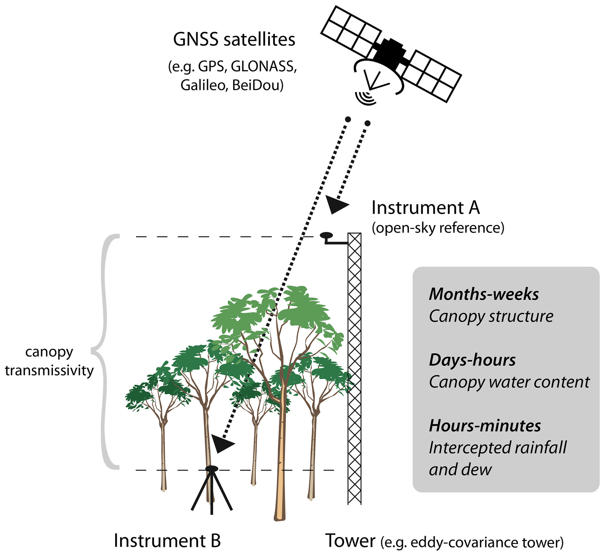
Figure 1 Instrument setup for measuring GNSS-based VOD. Each instrument consists of an antenna and a GNSS receiver.

The goal of this study is to demonstrate the potential of ground-based GNSS receivers for monitoring VOD, dry aboveground biomass, and water content continuously. In Sect. 2, we describe the measurements conducted at the study site and outline a simple canopy transmissivity model that is later used to estimate canopy density and water content from VOD measurements. Section 3 presents the raw GNSS measurements and the processing approach used to transform these into a canopy-averaged VOD time series. Section 4 compares the obtained seasonal and diurnal VOD time series against other in situ and satellite measurements. Section 5 provides an example of retrieval algorithm for aboveground biomass and canopy water content. Finally, Sect. 6 summarizes the main conclusions and provides some recommendations with respect to future deployments at existing ecohydrological sites.

2 Data and methods

2.1 Site setup

The experiment consists of a reference site that has an unobstructed view of the sky and a forested site that is located under a semi-closed forest canopy (Fig. 1). The open-sky reference site is located on the roof of a building of the California Institute of Technology in Pasadena, California (34.13624^∘ N, 118.12693^∘ W), and the forested site is located in the Huntington Library Botanical Garden, some 1.7 km away (34.12404^∘ , 118.11582^∘ W). The forested site is non-irrigated, with trees of about 5 to 15 m height. Tree species surrounding the antenna are mainly coast live oaks (Quercus agrifolia Née), and the understory is herbaceous. The overall climate is Mediterranean with weather conditions that are usually clear, daily maximum temperatures between 25 and 35 ^∘C, and low relative humidity. At each site a Septentrio PolaRx5e GNSS receiver, connected to a PolaNt-x MF right-hand circular polarized (RHCP) GNSS antenna, measured multi-constellation (GPS, GLONASS, Galileo, BeiDou) GNSS signals over the period of 13 May to 10 December 2020, with a logging rate of 15 s. Power loss at the site from 15 June to 1 July caused a data gap of 17 d. The raw GNSS data were quality-checked using the “teqc” pre-processing software, publicly available at the UNAVCO website (http://www.unavco.org/software, last access: 20 April 2023). The satellites' azimuth and elevation angles are also computed with teqc. Weather data are measured at the reference site by a station of the Total Carbon Column Observing Network (http://tccon-weather.caltech.edu/, last access: 20 April 2023). Weather data acquisition was interrupted from 15 to 26 July. Rainfall was measured with a tipping bucket at the Department of Public Works (DPW) HQ station (5 km from the forested site) by the Department of Public Works of the City of Los Angeles (https://dpw.lacounty.gov/wrd/rainfall/, last access: 20 April 2023).

2.2 Leaf water content

A total of 48 leaf samples were collected from two live oaks closest to the GNSS antenna on 18 October 2020, at 07:00, 12:00, and 17:00 LT (local time) using a 2 m long pruner. For each tree we equally sampled the same three different parts of the crown. Unless otherwise stated below, we followed the protocol advised in Mullan and Pietragalla (2012). Leaves were weighed on-site immediately after being sampled (fresh weight, FW) and stored individually in cooled glass vials. They were then transported to the lab where about 1 cm of water was added to each vial to cover the leaves' petioles. Turgid weight (TW) was measured after 12 h in a refrigerator (and in darkness). Then, the leaves were dried at 80 ^∘C for a period of 24 h, after which dry weight (DW) was measured. Relative leaf water content (RLWC, in percent) is calculated as follows:

$$\begin{array}{}\text{(2)}& \text{RLWC}={\displaystyle \frac{\text{FW}-\text{DW}}{\text{TW}-\text{DW}}}\times \mathrm{100}.\end{array}$$

We also calculate the gravimetric moisture content of the leaf (m_g, in g g⁻¹), a variable that is later used to model the leaf dielectric constant.

$$\begin{array}{}\text{(3)}& m_{\text{g}}={\displaystyle \frac{\text{FW}-\text{DW}}{\text{FW}}}\end{array}$$

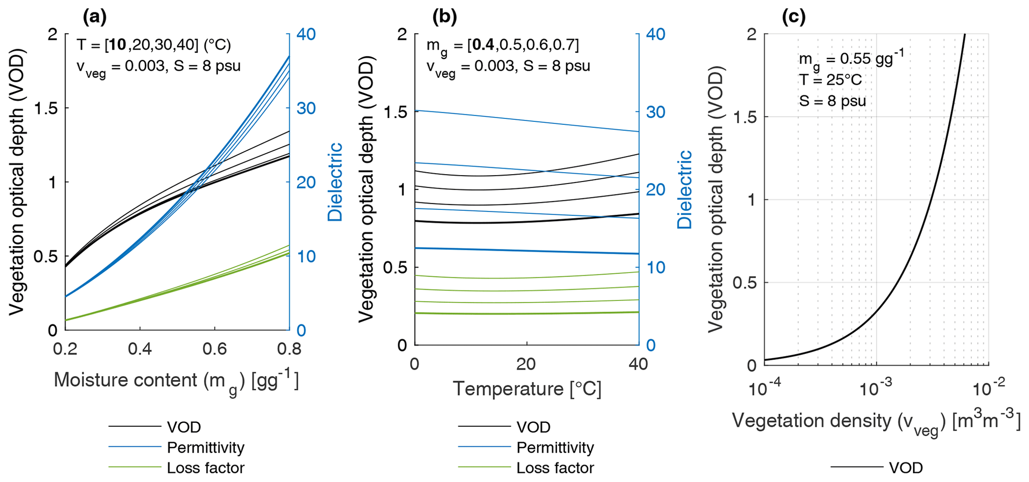
Figure 2 Modeled VOD at the GPS L1 frequency (1.575 GHz). (a–b) Modeled responses of canopy VOD and the vegetation material's dielectric properties to changes in gravimetric moisture content and temperature. The bold lines in (a) are obtained assuming a temperature of 10 ^∘C, with thin lines indicating 10 ^∘C increments. The bold lines in (b) are obtained assuming a gravimetric moisture content of 0.4 g g⁻¹, with thin lines indicating 0.1 g g⁻¹ increments. (c) Modeled response of canopy VOD to vegetation volumetric density. Canopy height is fixed at 7 m, and salinity is fixed at 8 ‰.

2.3 Canopy transmissivity model

We use a dielectric mixing model of the canopy transmissivity to investigate the potential roles of canopy volumetric density, water content, and temperature on the GNSS-based VOD measurements. We use a relatively simple formulation that only considers the attenuating effect of the canopy on the direct signal power and represents the canopy as a homogeneous layer, assumed to consist of randomly distributed elements (Ulaby and Jedlicka, 1984; Ulaby and Long, 2014; Guglielmetti et al., 2007). The transmissivity of the canopy is expressed as a function of a bulk canopy extinction coefficient (κ_e), canopy height (h, in meters), and incidence angle.

$$\begin{array}{}\text{(4)}& \mathit{\gamma }=e^{\frac{-\mathrm{2}{\mathit{\kappa }}_{\text{e}}h}{\cos \mathit{\theta }}}\end{array}$$

We define a fixed average canopy height of 7 m based on field observations. Neglecting scattering, the extinction coefficient is related to the complex index of refraction of the canopy layer (n_c^′′) (Ulaby and Long, 2014):

$$\begin{array}{}\text{(5)}& {\mathit{\kappa }}_e={\displaystyle \frac{\mathrm{2}\mathit{\pi }}{{\mathit{\lambda }}_{\mathrm{0}}}}{n}_{\text{c}}{}^{\prime \prime },\end{array}$$

where λ₀ is the free-space wavelength (in meters). Note that this formulation and the overall concept of bulk coefficients is applicable only when the inclusions in the canopy (i.e., the pockets of water within the vegetation tissues) are smaller in size compared to the observation wavelength (here λ₀≈19 cm for the GPS L1 frequency), meaning that scattering effects are small enough to be neglected (also see Jackson and Schmugge, 1991; Ulaby and Long, 2014). While this may be true for leaves, this assumption may not hold for larger elements such as branches and trunks. However, using a more complex theoretical scattering model, Guerriero et al. (2020) showed (for the case of a poplar forest) that the RHCP GNSS signals measured below a forest canopy are dominated by coherent attenuation, whereas only the left-hand circular polarized (LHCP) signals (which most geodetic ground-based GNSS antennas are designed to reject) are dominated by volume scattering. The complex index of refraction is calculated from the dielectric constant of the canopy layer (ε_c) (Ulaby and Long, 2014).

$$\begin{array}{}\text{(6)}& n_{\text{c}}{}^{\prime \prime }=-Im\left\{\sqrt{{\mathit{\epsilon }}_{\text{c}}}\right\},\end{array}$$

where Im indicates the imaginary part of a complex number. The canopy consists of two main phases: the surrounding air, which makes up most of the canopy volume, and the vegetation material. The dielectric of the canopy ε_c is calculated using a two-phase refractive mixing approach (Ulaby and Long, 2014, their Eq. 4.45):

$$\begin{array}{}\text{(7)}& \sqrt{{\mathit{\epsilon }}_{\text{c}}}=v_{\text{veg}}\sqrt{{\mathit{\epsilon }}_{\text{veg}}}+\left(\mathrm{1}-v_{\text{veg}}\right)\sqrt{{\mathit{\epsilon }}_{\text{air}}},\end{array}$$

where υ_veg represents the vegetation volumetric density, a parameter that may vary as a function of the growth cycle and is defined as the volume fraction of the vegetation material within the canopy (on the order of 0.0001–0.01 m³ m⁻³). This parameter is not to be confused with other measures of vegetation density like crown volume (i.e., including empty space) per meter squared. The term $\left(\mathrm{1}-v_{\text{veg}}\right)\sqrt{{\mathit{\epsilon }}_{\text{air}}}$ is practically equal to 1 with no imaginary part, such that Eq. (7) can be rewritten as follows (Ulaby and Long, 2014, their Eq. 11.89):

$$\begin{array}{}\text{(8)}& n_{\text{c}}{}^{\prime \prime }\approx -Im\left\{\sqrt{{\mathit{\epsilon }}_{\text{veg}}}\right\}{v}_{\text{veg}}.\end{array}$$

The dielectric of the vegetation (ε_veg) incorporates a real and an imaginary part, namely the dielectric permittivity and the dielectric loss (${\mathit{\epsilon }}_{\text{veg}}={\mathit{\epsilon }}_{\text{veg}}{}^{\prime }-i{\mathit{\epsilon }}_{\text{veg}}{}^{\prime \prime })$. Both depend on various factors, but the most important ones are the considered wavelength, the vegetation water content, and the plant water's temperature and ionic conductivity. Here we model ε_veg using the semi-empirical model for vegetation introduced by Ulaby and El-rayes (1987) and valid over the range 0.2–20 GHz. This model is derived from an observational dataset of corn leaves and has been successfully used for a wide range of species, including trees (e.g., Chuah et al., 1995). The model expresses the dielectric of the vegetation ε_veg as a function of its gravimetric moisture (m_g), its temperature, and its salinity. The numerous equations are not reported here but can be found for instance in Ulaby and El-rayes (1987) and Ulaby and Long (2014).

The purpose of the transmissivity and dielectric models described above is to provide a simple estimate of the potential effects of canopy density, temperature and water content changes on canopy transmissivity. It is important to note that this simple formulation neglects several aspects, including volume scattering, which may be important in configurations with denser biomass (and also when interpreting LHCP backscatter or LHCP signals). In Fig. 2, we illustrate the modeled VOD response (at the GPS L1 1.575 GHz frequency) to potential changes in vegetation water content, temperature, and vegetation volumetric density. As expected, an increase in vegetation moisture content (Fig. 2a) leads to a substantial increase in the vegetation's dielectric permittivity and dielectric loss, which results in a lower canopy transmissivity. Temperature influences the vegetation's dielectric properties as well, albeit less markedly (Fig. 2b). The ionic conductivity of the plant water is the main factor explaining the slight dependency of the loss factor (and of VOD) on the temperature. Finally, vegetation volumetric density within the canopy is also a parameter that strongly controls the transmissivity (Fig. 2c). Note that the shape of these response curves (the response to temperature in particular) may change depending on the considered frequency.

2.4 GNSS data processing

2.4.1 Raw SNR observations

Most survey-grade GNSS receivers commonly register signal-to-noise ratios (SNR, in dB), which express the magnitude of the received signal power from each satellite compared to the background noise (Bilich et al., 2007). The quantity logged by the Septentrio receiver is the carrier-to-noise density ratio (C $/$ N₀), which we report as SNR for simplicity, assuming a 1 Hz bandwidth (Larson and Nievinski, 2012). The hemispherical plot in Fig. 3a illustrates the SNR values measured over the course of a single day at the reference (open-sky) station for just one satellite of the GPS constellation (PRN2). GNSS satellites are commonly identified by their pseudorandom code (PRN), which allows the receiver to determine which satellite is being tracked, such that its azimuth and elevation can be calculated. Individual satellite tracks repeat after a period that depends on the GNSS constellation (e.g., twice per sidereal day (23 h and 56 min) for GPS and every 10 sidereal days for Galileo). As is very commonly observed, the SNR increases as the satellite rises up above the horizon (12:00 LT), reaches its peak value at maximum elevation (14:00 LT), where the antenna gain is the strongest, and decreases again until the satellite disappears from view (17:00 LT). As can be seen from Fig. 3b, the same satellite track observed from the forested site shows numerous drops in SNR. Assuming a comparable level of background noise at the two sites, the SNR difference between the two sites (ΔSNR, Eq. 9) reflects, for the most part, the transmissivity of the canopy, expressed in decibels. As expected, it is mostly negative (Fig. 3c–d), indicating attenuation by the forest canopy.

$$\begin{array}{}\text{(9)}& \mathrm{\Delta }\text{SNR}={\text{SNR}}_{\text{Forested}}-{\text{SNR}}_{\text{OpenSky}}\end{array}$$

Combining all available data (May to December 2021) from 102 individual GNSS satellites, we produce a hemispherical map of the average ΔSNR (Fig. 4a), which matches the overall distribution of canopy density as seen from the antenna location (Fig. 4b). Note that absolute SNR values vary from spacecraft to spacecraft, as those have different (and occasionally time-varying) transmit powers. It is thus very important to first pair the individual SNR measurements taken by the two receivers and only then average any ΔSNR values.

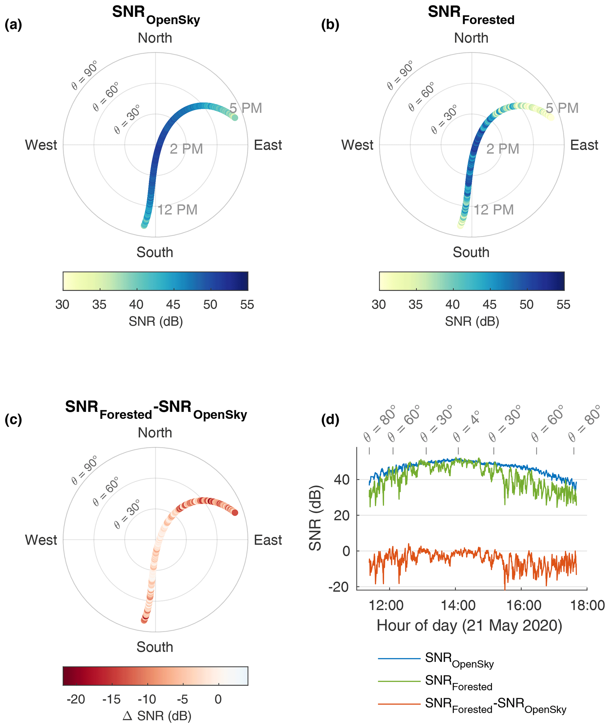
Figure 3 Sky plots illustrating the SNR observations on 21 May 2020 for one specific GPS satellite (PRN2) at the open-sky site (a) and the forested site (b). (c) Difference in SNR between the two sites. (d) The same as (a–c) but showing the temporal evolution of the SNR. The center of the polar plots corresponds to the local zenith.

It should be noted that while the SNR measurement is dominated by the contribution of the direct (line-of-sight) signal, it also includes a comparatively weaker contribution from volume scattering and indirect ground multipath reflections (Bilich et al., 2007; Smyrnaios et al., 2013), the latter of which may contain information about, for instance, soil water status (Larson, 2016). Ground multipath often manifests itself as a periodic oscillation of the SNR, which is caused by the successively constructive and destructive interference from ground reflections, as a function of the satellite's elevation angle. Such periodic oscillations of a few decibels are barely visible for instance in Fig. 3d at the beginning and the end of the SNR_OpenSky time series (blue curve), where the roof's floor acts as the reflector. However, while present in our data, ground multipath represents a signal that is about an order of magnitude smaller than the attenuations caused by the presence of trees in the line of sight. It is only in some favorable situations (e.g., flat grasslands, areas of open water), where large flat surfaces surrounding the antenna produce a coherent structure in ground reflections, that multipath is strong enough to be reliably detected in SNR, even though our GNSS systems are explicitly designed to reject such signals. Indeed, most geodetic-grade antennas have metal ground planes and are much less sensitive to the predominantly left-hand circular polarized (LHCP) ground reflections of the transmitted right-hand circular polarized (RHCP) signal (note that, in contrast, spaceborne GNSS reflectometry also relies on the LHCP signal). Thus, in our case, the difference in SNR between the two sites is predominantly due to the attenuation of the direct RHCP signal by the forest canopy, and it is reasonable to assume that ground multipath effects are of the second order. This is also confirmed by a ΔSNR close to zero in the sky sectors where the canopy is either absent or very sparse (Fig. 4). It is only when the incidence angle is larger than 80^∘ that the majority of the reflected GNSS signal is co-polarized (RHCP) (Smyrnaios et al., 2013). As a precaution, we discard all observations with an incidence angle higher than 80^∘ for the remainder of the analysis.

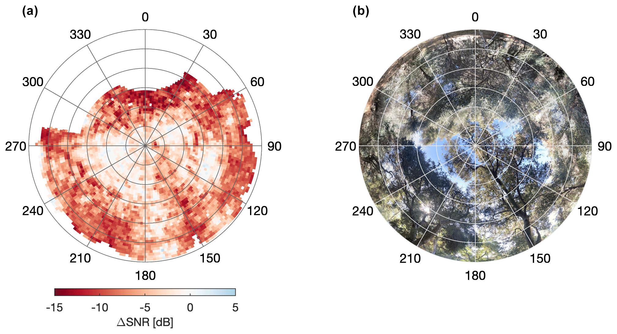
Figure 4 (a) Sky plot illustrating the mean SNR difference between the open sky and the forested site for L1 and L1C signals ($n=\mathrm{2.17}\times {\mathrm{10}}^{\mathrm{7}}$ observations, taken over an 8-month period). The mean value within each 2^∘ equal-area sky sector is shown. Some sky sectors in (a) are obstructed by buildings at the reference site and are thus excluded from the analysis (towards the northwest and northeast). (b) Hemispheric photograph taken from the perspective of the forested site antenna.

2.5 Transmissivity and vegetation optical depth

After conversion from decibels to a linear scale (Eq. 10), the ΔSNR measurements are used as the transmissivity estimate, and VOD is calculated from Eq. (11). Note that in our case this represents L-band VOD at RHCP polarization.

$$\begin{array}{}\text{(10)}& {\displaystyle }\mathit{\gamma }={\mathrm{10}}^{\frac{\mathrm{\Delta }\text{SNR}}{\mathrm{10}}}\text{(11)}& {\displaystyle }\text{VOD}=-\ln \left(\mathit{\gamma }\right)\cos \mathit{\theta }\end{array}$$

The resulting hemispherical distribution of long-term mean transmissivity and VOD is reported in Fig. 5a–b. In some cases, the instantaneous transmissivity values computed from the raw GNSS measurements were higher than 1, leading to a VOD lower than zero (about 8 % of all measurements). This occurs because individual SNR measurements unavoidably include some random noise and non-random multipath interferences that can cause the measured signal power at the reference site to be transiently lower than at the forested site. This especially occurs where there are gaps in the canopy and both antennas have a clear line of sight to the satellite. To preserve the error structure of the measurements, we propose to still use these values when computing temporal (i.e., daily or hourly) averages later in the paper so that positive and negative errors can cancel out, avoiding a potential bias in our estimate of the average VOD (Fig. 5b). While transmissivity has an obvious dependence on the incidence angle (Fig. 5c), this is not the case for VOD (Fig. 5d), as would be expected from Eq. (1). The strong anisotropy of the long-term VOD pattern (Fig. 5b) reflects the heterogeneous structure of the canopy (Fig. 4b), with local mean VOD values ranging from 0.16 to 2.46 (1st and 99th percentiles) depending on the azimuth and incidence angle. The whole canopy average VOD is 0.79, which is similar to what is reported for evergreen broadleaf forests at L band (Konings et al., 2017a).

Figure 5 Sky plot illustrating the mean canopy transmissivity (a) and mean VOD (b). The mean value within each 2^∘ equal-area sky sector is shown. (c–d) The box plots show the distribution (minimum, 25th, 50th, 75th percentiles, and maximum) of all individual transmissivity and VOD measurements ($n=\mathrm{2.17}\times {\mathrm{10}}^{\mathrm{7}})$ as a function of the incidence angle (relative to zenith).

2.6 Computation of VOD time series

Because changes in VOD over time may provide valuable information about the vegetation's growth cycle and water content, it is of great interest to investigate its temporal evolution. However, this is complicated by the patterns of GNSS orbits, which change continuously. In Fig. 6a, we provide an overview of the most frequent orbit patterns over our site and their mean revisit time, showing which sky sectors are most often observed. While it takes about a day on average to cover most of the observable sky sectors (Fig. 6b, red curve), monitoring one specific section of the canopy every 1 or 2 h would only be possible over a narrow band where many satellite tracks coincide (Fig. 6a). Note that the location of the highly sampled band (and the blind spot above it) depends on the site's latitude (it is closer to zenith at higher latitudes) and would be located on the opposite side in the Southern Hemisphere. In practice, this means that a continuous (gap-free) and robust VOD time series can only be obtained by aggregating data collected at different azimuth and elevation angles (i.e., trading angular resolution for temporal coverage). However, as different cross-sections within Fig. 5b are observed each day, the changing and irregular sampling of the canopy introduces spurious variability in daily site-averaged VOD. When calculating sub-daily (e.g., hourly) time series, this problem is even more important and will obfuscate most of the potential real variability. For example, binning the raw GNSS-based VOD observations into hourly averages produces a rather noisy time series with just seasonal trends visible (Fig. 7a–b, “VOD raw”). This is because a lot of the variability in VOD raw is caused by the fact that different areas of a heterogenous canopy are observed every hour. This issue can also be diagnosed quantitatively. For instance, computing the serial autocorrelation² of the raw VOD time series (Fig. 7c) reveals periodicities likely not related to ecohydrological processes but instead caused by the combined repeat times of the different GNSS constellations.

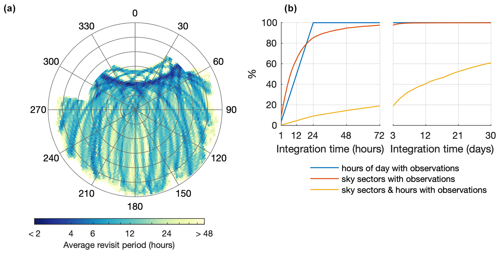
Figure 6 (a) Sky plot illustrating the mean revisit time (average number of hours until the next overpass within a given sky sector). This includes the GPS, GLONASS, Galileo, and BeiDou constellations. (b) Average sampling statistics as a function of data integration time. For instance, 84 % of all observable sky sectors are observed at least once after 24 h of continuous measurements (red curve). After 30 d of continuous measurement, 62 % of all observable sky sectors and hours of the day have been observed at least once (yellow curve).

Here, we propose addressing this sampling problem by subtracting the long-term average (similar to what is shown in Fig. 5b) taken at the same azimuth and incidence angle from each individual VOD observation. The goal is to subtract the angular heterogeneity in VOD, representing the uneven canopy distribution, and only retain residuals from the locally averaged attenuation (Eq. 12). The long-term average at a given incidence angle and azimuth (Eq. 13) is calculated inside a neighborhood N_i that includes all measurements within some chosen angular distance δ from that point of interest (Eq. 14).

$$\begin{array}{}\text{(12)}& {\displaystyle }{\text{VOD}}_{{\mathit{\phi }}_i,{\mathit{\theta }}_i,t_i}^{\text{residual}}={\text{VOD}}_{{\mathit{\phi }}_i,{\mathit{\theta }}_i,t_i}-{\text{VOD}}_{{\mathit{\phi }}_i,{\mathit{\theta }}_i}^{\text{mean}}\text{(13)}& {\displaystyle }{\text{VOD}}_{{\mathit{\phi }}_i,{\mathit{\theta }}_i}^{\text{mean}}={\displaystyle \frac{\mathrm{1}}{n}}\sum _{j=\mathrm{1}}^n\left({\text{VOD}}_{{\mathit{\phi }}_j\in N_i,{\mathit{\theta }}_j\in N_i}\right)\text{(14)}& {\displaystyle }\begin{array}{rl}{N}_i:\text{hav}& \left({\mathit{\lambda }}_i-{\mathit{\lambda }}_j\right)+\cos \left({\mathit{\lambda }}_i\right)\cos \left({\mathit{\lambda }}_j\right)\\ \text{hav}& \left({\mathit{\phi }}_i-{\mathit{\phi }}_j\right)<\text{hav}\left(\mathit{\delta }\right)\end{array}\end{array}$$

Here the terms φ_i, λ_i, and t_i represent the azimuth, elevation, and time step of the point of interest (for angles expressed in degrees, $\mathit{\lambda }=\mathrm{90}-\mathit{\theta })$. Equation (14) is the condition that determines if measurements belong to the neighborhood around the point of interest “i”. The left term in Eq. (14) is the formula for the haversine of the angle between any two points on a sphere. The right term is the haversine of a chosen angle δ, which defines the extent of the neighborhood.

An adequate value for δ may be selected based on the autocorrelation of the VOD observations with respect to the angular distance (Fig. S1 in the Supplement). The results suggest that there is a high consistency of the VOD estimates up to an angular distance of about 0.5 to 1^∘. Figure S1 also provides some indication of the repeatability of the measurements when taken at an interval of several days. As can be expected, observations separated by a longer temporal interval are in lower agreement. The selection of δ is ultimately a compromise between obtaining an accurate long-term VOD average while still retaining enough observations within the neighborhood. In our case, we found that $\mathit{\delta }=\mathrm{0.5}{}^{\circ }$ seems to be an adequate value. To avoid excessive computations, we calculate ${\text{VOD}}_{{\mathit{\phi }}_i,{\mathit{\theta }}_i}^{\text{mean}}$ at each node of a fine hemispherical grid with a spacing of 0.1^∘. The ${\text{VOD}}_{{\mathit{\phi }}_i,{\mathit{\theta }}_i}^{\text{mean}}$ value closest to each individual ${\text{VOD}}_{{\mathit{\phi }}_i,{\mathit{\theta }}_i,t_i}$ is then used in Eq. (12). Binning the calculated VOD residuals into hourly averages, we produce a processed time series of the average VOD (Fig. 7, “VOD processed”). To preserve the original absolute level of VOD, the average ${\text{VOD}}_{{\mathit{\phi }}_i,{\mathit{\theta }}_i}^{\text{mean}}$ (across all φ and θ) is added back to the residual time series (otherwise the “VOD processed” time series would be centered around zero). The serial autocorrelation of that processed time series (Fig. 7d) is now dominated by a more credible 24 h cycle.

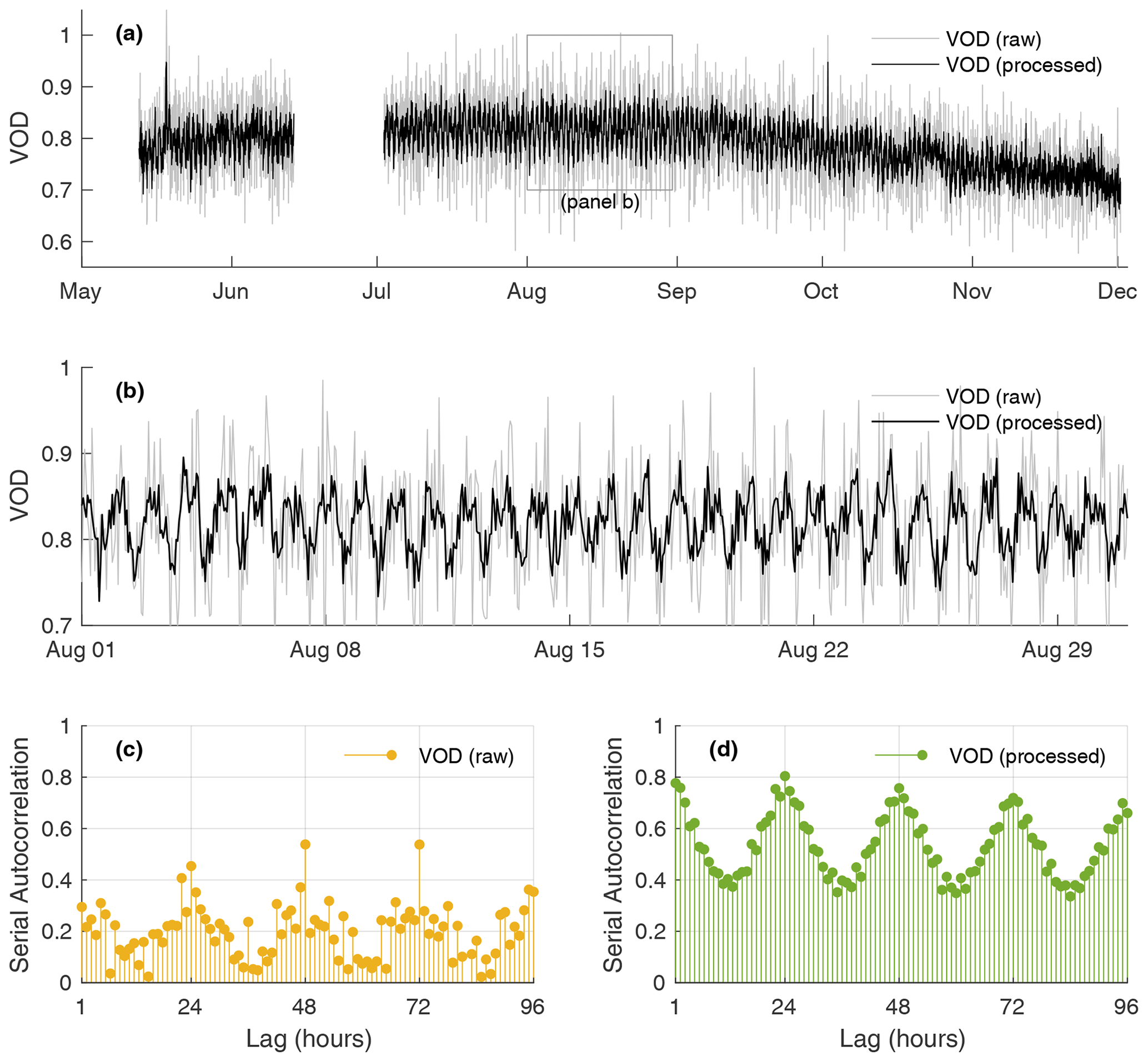
Figure 7 (a) Hourly time series of VOD before and after reducing the impact of irregular sampling caused by the GNSS orbit patterns. (b) Zoom on August showing sub-daily variability in VOD. (c–d) Serial autocorrelation of the raw and processed VOD time series.

3 GNSS-based vegetation optical depth

3.1 Seasonal changes

In Fig. 8, we compare processed daily VOD averages against other observations. Using quality-checked 30 m satellite images from Sentinel-2 (Claverie et al., 2018), we calculate the EVI (Liu and Huete, 1995) at our site (Fig. 8a). EVI is a commonly used vegetation index and an overall proxy for vegetation greenness, health, and photosynthetic activity. Generally, we find that the temporal evolution of VOD appears to lag behind that of EVI by about 2 months. This is consistent with previous findings over drylands by Tian et al. (2016), who found a temporal shift (increasing as a function of forest density) between satellite-based VOD and vegetation greenness. They suggest that this may be explained by the longer growing season and later peak time of woody plants compared to the herbaceous understory. Similar lags between peak NDVI and peak VOD have been observed in other regions of the world from satellite data (Wang et al., 2020; Tian et al., 2018). The peak EVI in June coincides with the maximum in available solar energy (Fig. 8b), and with an increase in VOD, which could suggest a buildup of biomass in the canopy. This is followed by a slow decline in EVI that does not occur in VOD until the end of August. The gradual decline in vegetation activity and health over the summer is typical of the region and is mainly a response to the overall increase in water stress resulting from warmer temperatures, drier atmosphere, and low soil moisture after months with no rainfall. The 2020 summer culminated with a record-breaking heat wave on 6 September (Fig. 8c), followed by a steady decline in VOD during the fall season where some minor shedding of leaves could be observed at the site.

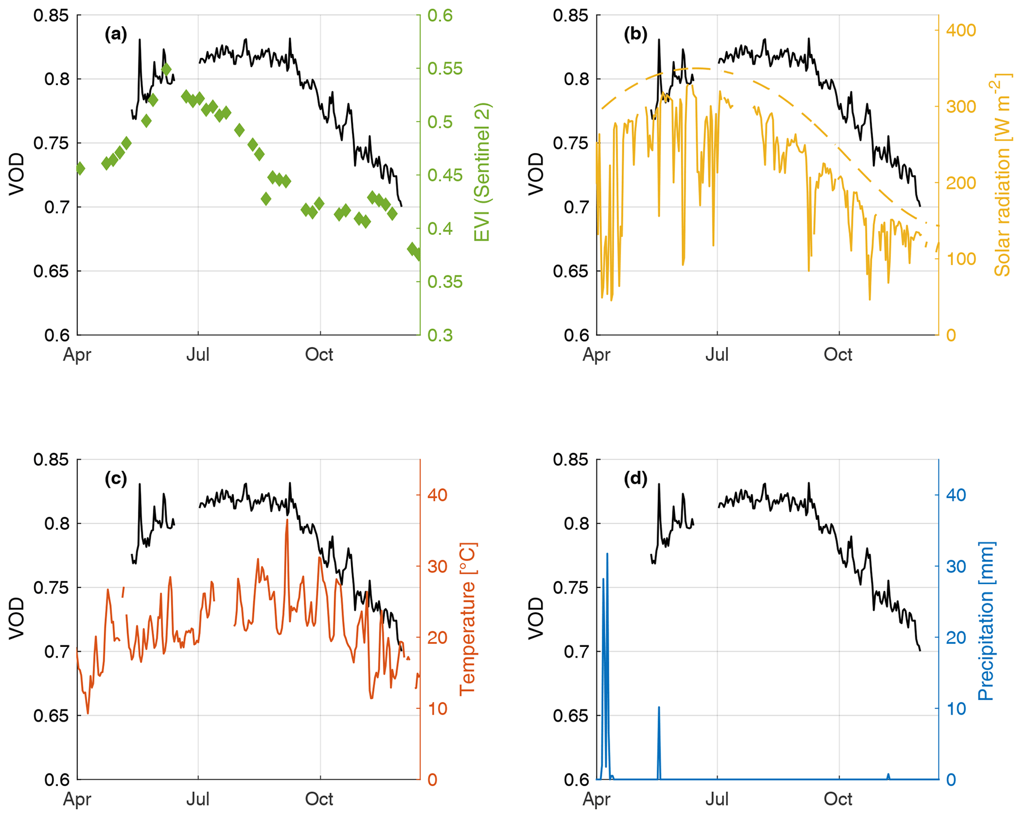
Figure 8 Daily time series of GNSS-based VOD compared against (a) Enhanced Vegetation Index calculated from harmonized Sentinel-2 images (HLS v1.4, 30 m resolution, https://hls.gsfc.nasa.gov/, last access: 20 April 2023), (b) solar and potential solar radiation observed at the reference site, (c) air temperature observed at the reference site, and (d) precipitation totals measured at the closest rain gauge station.

3.2 Diurnal cycle

Even though processed hourly VOD time series contain a certain amount of noise (e.g., Fig. 7b), they also show a relatively strong 24 h cycle (Fig. 7d). One way of obtaining a more robust and precise estimate of that diurnal cycle is to calculate the average diurnal cycle from data aggregated over a long period of time, e.g., several days or even a whole month. This is what is done in Fig. 9a. The average diurnal cycle of VOD is consistent with what would be expected from the perspective of plant physiology and its response to water stress over the course of a typical day. VOD culminates in the early hours of the morning (at around 05:00 to 06:00 LT), indicating a relatively “water-rich” canopy, because leaves and stems have been replenished with water overnight and likely also due to the occasional presence of dew in the canopy. This peak is followed by a gradual drop after sunrise (at about 06:00 LT), concurrent with the onset of photosynthesis and transpiration, as well as an increase in vapor pressure deficit (i.e., an increase in atmospheric water demand). As a result, dew quickly evaporates and the vegetation starts losing more water through transpiration, thus depleting canopy water content. Around noon, some equilibrium is reached between plant water losses and plant water supply so that VOD becomes relatively stable. In the evening, plant rehydration causes VOD to rise back.

A minor peak in VOD is observed at around 15:00 LT but remains difficult to explain without further evidence. That peak might indicate a brief period of canopy rehydration, documented for instance in Douglas firs (Cermak et al., 2007, their Fig. 6), resulting from midday stomatal closure (Xiao et al., 2021). The associated “midday depression” of transpiration and photosynthetic rates has been widely documented (e.g., Faria et al., 1996; Kamakura et al., 2011). However, theory (Fig. 2b) also predicts that VOD could slightly increase in response to higher canopy temperature, which would peak at about that time of the day. In Sect. 4.2, we present an attempt to disentangle these two possible contributions.

Overall, our results agree with previous observations of a diurnal cycle in VOD and backscatter (e.g., Konings et al., 2017b; Holtzman et al., 2021; Vermunt et al., 2021; Prigent et al., 2022). Such diurnal VOD changes are consistent with our knowledge of canopy water storage dynamics, as derived from either continuous direct measurements (Zhou et al., 2018) or from the imbalance between plant water losses (i.e., transpiration) and plant water supply (i.e., measured with sap flow sensors) (Kocher et al., 2013; Cermak et al., 2007). The leaf samples collected on the site in October also confirm that some intraday variability exists in relative leaf water content (Fig. 9b). Monitoring the diurnal cycle of plant water status is interesting because it can provide key information about plant hydraulic traits (Konings and Gentine, 2016) and enables disentangling the effects of limitations in root water uptake, plant transpiration, and water redistribution within the plant (Konings et al., 2021). In Fig. 9c, we investigate whether our method would be able to monitor such physiologically relevant changes, specifically seasonal changes in pre-dawn versus midday water status. We find midday VOD to be almost always lower than pre-dawn VOD, a behavior that is entirely consistent with field observations of pre-dawn and midday leaf water potentials (Martínez-Vilalta et al., 2014). Seasonally, both pre-dawn and midday VOD start to decrease in September with the start of a very dry period during which the vapor pressure deficit (VPD) remains high even during the night. Pre-dawn and midday VOD are significantly correlated with each other (r=0.79), as is frequently observed with leaf water potential; however, we note that this might also occur (at least partly) because VOD is sensitive not only to relative changes in water content but also to potential seasonal changes in the absolute amount of biomass present in the canopy (Momen et al., 2017). These mixed contributions from both absolute biomass and its relative water content are even better illustrated in Fig. 9d, where we find that the amplitude of the diurnal cycle in VOD becomes larger as denser sections of the canopy are considered.

Figure 9 (a) Average diurnal cycle for the month of August. Average VOD (black) is shown at a 15 min sampling rate with shaded areas delineating the 25th and 75th percentiles. VPD and surface wetness data from the TCCON weather station have hourly resolution. (b) Average diurnal cycle for the month of October compared with in situ measurements of relative leaf water content. (c) Daily pre-dawn and midday VOD, calculated using all observations within the windows 04:00–06:00 and 12:00–14:00 LT, respectively. (d) Diurnal VOD anomaly (centered around zero) measured for progressively denser classes of canopy (based on the long-term VOD average; see Fig. 5b).

4 Retrieval of canopy density and water content

4.1 Approach and algorithm

In the following, we demonstrate an approach to retrieve changes in canopy density and water content at hourly resolution based on the transmissivity model presented in Sect. 2.3. Combining Eqs. (1), (4), (5), and (8) we obtain the following expression for modeled VOD^′:

$$\begin{array}{}\text{(15)}& {\text{VOD}}_t^{\prime }=\mathrm{2}{k}_{\text{e}}h=\mathrm{2}{\displaystyle \frac{\mathrm{2}\mathit{\pi }}{{\mathit{\lambda }}_{\mathrm{0}}}}\left[-Im\left\{\sqrt{{\mathit{\epsilon }}_{{\text{veg}}_t}}\right\}\right]v_{{\text{veg}}_t}h.\end{array}$$

Canopy height h is 7 m, and λ₀ is the free-space wavelength. This leaves the following items as free parameters: $v_{{\text{veg}}_t}$, the time-dependent vegetation volumetric density (in m³ m⁻³), and ${\mathit{\epsilon }}_{{\text{veg}}_t}$, the time-dependent bulk dielectric constant of the vegetation, which is itself a function of the (measured) temperature, (unknown) water content (m_g), and (unknown) salinity of the plant water (Ulaby and El-rayes, 1987). A similar expression may be found, for instance, in Kerr and Wigneron (1995) or Guglielmetti et al. (2007).

Here, we use the canopy-averaged processed VOD time series (i.e., Fig. 7b) as the observed VOD. This means that canopy density and water content are assumed to evolve homogeneously over the whole canopy. If the forest canopy is very heterogeneous, this might not be a suitable approximation. For instance, some groups of trees may evolve at different speeds, or individual trees may exhibit different responses to water stress. If this is suspected, a retrieval may be performed for each individual tree, potentially at the cost of retrieval accuracy since fewer observations will be available. In practice, this would mean separating the field of view of the antenna into subsectors (e.g., based on data similar to Fig. 4) and computing a processed VOD time series for each subsector. However, for the sake of simplicity this is not done here, and we perform only one retrieval for the whole canopy.

Disentangling the effects of changes in overall biomass density (v_veg) versus variations in water content (m_g) is one of the main challenges when trying to interpret and better understand VOD (Momen et al., 2017; Konings et al., 2019). Because changes in biomass tend to unfold at a much slower pace than changes in relative water content, a common strategy has been to assume that long-term changes in VOD are mostly related to biomass, while short-term changes (and especially a diurnal signal) are most likely due to variations in water content (e.g., Konings et al., 2016). In the retrieval detailed below, we will make use of this assumption and allow v_veg to contain only low-frequency (long-term) changes. We also assume that the temperature of the canopy can be approximated by the air temperature. While leaf and air temperatures are not necessarily equal, as documented by many field studies, an error of a few degrees is negligible for the purpose of calculating ε_veg (Fig. 2b), and our main purpose is only to gain a reasonable representation of the seasonal and diurnal effects of temperature on the dielectric constant. We also note that these temperature impacts on the dielectric are often neglected in other studies.

Finally, the plant water salinity is also unknown in our case, but it is most likely within a range of about 1 to 11 psu according to previous experience (Ulaby and Long, 2014). In the absence of any other data, we assume that salinity is constant over the whole time period. In our retrieval algorithm, a range of a priori values for vegetation water salinity is tested, and the value yielding the best overall (season) fit to the observed VOD data is selected as the most plausible. We note that salinity, in the context of the dielectric model of Ulaby and El-rayes (1987), is meant to account for the ionic conductivity of the plant water (due to both sugars and salts). Thus, the salinity yielding the best fit might not necessarily reflect the actual (NaCl) salinity of the plant water.

Below, we summarize the retrieval algorithm step by step. The root-mean-squared error between modeled and observed VOD is always used as the cost function, and optimization at steps 2 and 4 is carried out with a simplex search method. We define the search space for m_g, the gravimetric moisture content as [0.3, 0.7]. This is guided by the average values measured at the site (m_g=0.45 ± 0.02 g g⁻¹), and also by data from Scoffoni et al. (2014) for Quercus agrifolia in the Los Angeles area (m_g=0.48 g g⁻¹). The search space for v_veg (volume of vegetation material per cubic meter) is loosely defined as [0.0001, 0.01 m³ m⁻³] based on the indications of Ulaby and Long (2014).

Algorithm

1. Select an a priori value for salinity.

2. For each 24 h period, optimize v_veg (one value for the entire 24 h period) together with m_g (24 individual hourly values). The result is a time series of daily v_veg and hourly m_g covering the whole season (Fig. 10a).

3. Filter the time series of v_veg with a low-pass filter. Here we use a local regression filter (LOESS) with ±30 d width (Fig. 10a).

4. Optimize m_g using the new v_veg values obtained at step 3 (Fig. 10b).

5. Filter the time series of m_g to reduce the high-frequency noise. Here we use a LOESS filter with ±2 h width (Fig. 10b).

6. Evaluate the agreement between the modeled and observed canopy-averaged VOD time series (with v_veg and m_g from steps 3 and 5) and determine an optimal salinity (Fig. 10c).

Because v_veg is kept constant only for the duration of a day, there is some high-frequency variability in the v_veg time series that is obtained after step 2 (Fig. 10a). These sudden and unrealistic jumps in v_veg also contaminate the estimates of m_g (not shown). These problems are alleviated in step 3, where daily estimates of v_veg are low-pass filtered, consistent with the assumption that changes in biomass usually occur at a relatively slow pace. Note that although calibrating v_veg over a time period longer than a day would also smooth the estimate, we found that optimizing v_veg at a daily time step and then applying a low-pass filter was much more effective in mitigating the influence of outliers. A new hourly time series of m_g is then obtained based on the filtered v_veg time series in step 4 (Fig. 10b). Because the m_g time series is contaminated by some noise inherited from the VOD observations, some mild smoothing is applied to m_g in step 5 (Fig. 10b). Steps 2 to 5 are repeated for different values of salinity, and we retain the optimum of the cost function as the most likely value (Fig. 10c). Here we find an optimum with a salinity of 8.9 psu, which is a physically plausible value.

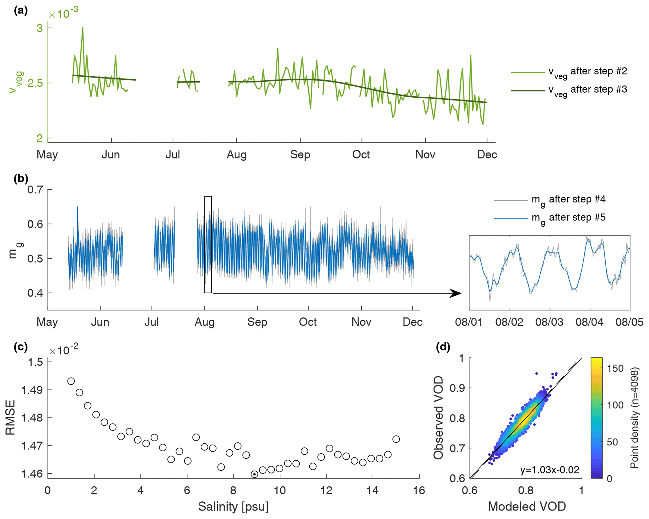
Figure 10 (a) Time series of v_veg after steps 2 and 3. (b) Time series of m_g after steps 4 and 5 with a zoom on a short period for better visibility. (c) Root-mean-squared error obtained for various salinity values. (d) Scatter plot of the modeled versus observed VOD. The data shown in (a), (b), and (d) are based on a salinity of 8.9 psu.

Before we interpret these results, some limitations to the presented approach need to be emphasized. First, the dielectric model of Ulaby and El-rayes (1987) was originally developed for leaves; however, it is clear that branches and stems also contribute to canopy extinction. To our advantage, however, Kurum et al. (2009a) have determined with numerical simulations (at L band) that leaves do have a significant impact on extinction, while branches have a dominant contribution only in terms of backscatter, and trunks have a negligible impact on extinction. Steele-Dunne et al. (2012) arrived at similar conclusions and concluded that leaf moisture is by far the dominant control on vegetation transmissivity at L band for both polarizations (but see Ferrazzoli and Guerriero, 1996, for a different perspective). Observations by Mätzler (1994) in a deciduous forest also showed a clear dependence of the transmissivity on the presence or absence of leaves in the canopy. It is assumed that the dielectric model of leaves and its sensitivity to moisture, temperature, and salinity provides a sufficient approximation for the behavior of the whole crown (branches and stems included). However, the impact of intercepted water (due to dew deposition or rainfall) is not explicitly represented and will thus be compensated for by an overestimation of the retrieved gravimetric moisture content. There is unfortunately not enough empirical data in our case to also retrieve intercepted water independently.

4.2 Results and interpretation

In Fig. 11a, the retrieval of gravimetric moisture content (m_g) is compared against observations of leaves taken at the site on 18 October. There is a bias of 0.04 g g⁻¹ between the retrieval and the observations, a surprisingly good performance given the assumptions made during the retrieval of m_g and the fact that a few leaf samples are not necessarily representative of the entire canopy. The relative difference between dawn and daytime values (about 0.03 g g⁻¹) is consistent between the retrieval and the observations. We also find that the relationship between retrieved hourly m_g and VPD becomes narrower (Fig. 11b) compared to the relationship between hourly VOD and VPD (Fig. 11c). Even though this does not provide any formal validation of the m_g retrieval, it does suggest that the retrieval is somewhat successful in concentrating in m_g a response to atmospheric water demand that is consistent with observed plant stomatal behavior (e.g., Grossiord et al., 2020).

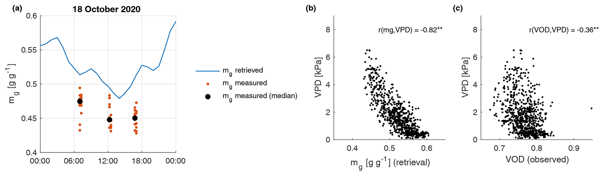
Figure 11 Retrieved and measured values of gravimetric moisture content (m_g) on 18 October (a). Scatter plots of the hourly values of m_g (b) and VOD (c) against vapor pressure deficit (VPD) for the month of October (both correlations are significant at p<0.01).

Dry aboveground biomass (AGB, kg m⁻²) can be calculated by multiplying the retrieved volume of the vegetation material (v_veg×h, m³ m⁻²) by the average density of the dry leaf material (ρ_dry). Here we use leaf density to remain consistent with the model's assumptions, but it is unknown if the density of leaves, branches, wood, or some weighted average of all three would be more relevant at this stage. We use a value of ρ_dry=630 kg m⁻³ reported by Scoffoni et al. (2014) for Quercus agrifolia.

$$\begin{array}{}\text{(16)}& \text{AGB}=v_{\text{veg}}h{\mathit{\rho }}_{\text{dry}}\end{array}$$

Canopy water content (CWC) is then calculated as follows:

$$\begin{array}{}\text{(17)}& {\displaystyle }{m}_{\text{g}}={\displaystyle \frac{\text{water weight}}{\text{fresh weight}}}={\displaystyle \frac{\text{CWC}}{\text{CWC}+\text{AGB}}},\text{(18)}& {\displaystyle }\text{CWC}={\displaystyle \frac{\text{AGB}{m}_{\text{g}}}{(\mathrm{1}-m_{\text{g}})}}.\end{array}$$

The resulting time series are shown in Fig. 12a. For AGB, we obtain a mean value of 10.9 kg m⁻² with very little seasonal variation, as may be expected for an evergreen forest. Note that this estimate should be interpreted with the awareness that VOD-based estimates of AGB likely do not weigh all canopy constituents evenly. While L-band VOD is sensitive to leaves, the sensitivity to branches and trunks increases at lower leaf moisture content (Steele-Dunne et al., 2012) or if leaves are entirely absent. Because in situ estimates of AGB are not available at our experimental site, we can only put this value into the context of the literature. Several studies have empirically linked VOD observations to global AGB datasets that are based on satellite data and forest inventories (Avitabile et al., 2016). For instance, using the exponential relationship calibrated at L band by Vittucci et al. (2019), we obtain (for an average VOD value of 0.79 at our site) an AGB of 13.8 kg m⁻², which is not so far from our estimate. Other results from Brandt et al. (2018) suggest a linear relationship between AGB and L-band VOD, with a sensitivity of about 133 Mg ha⁻¹ per unit of VOD, which would yield an AGB of 10.5 kg m⁻² at our site. Thus, existing empirical relationships between VOD and AGB would suggest that the results obtained with the retrieval algorithm and its simple model are reasonable.

In terms of canopy water content (CWC), which is a function of both m_g and AGB, we find a long-term mean of 12.1 kg m⁻² at our site. As for AGB, it is important to keep in mind that the CWC estimate does not weigh all canopy constituents evenly. In addition, our retrieval assumes that the attenuation is dominated by small canopy elements, even though the contribution of large elements (like large branches or trunks) to CWC is likely not negligible. Comparisons with other studies are quite difficult here because the relationship between VOD and vegetation water content is poorly known for forests. Many studies over grasslands and croplands have demonstrated an empirical linear relationship of the form $\text{VOD}=b\times \text{CWC}$. However, b is also known to be vegetation and time dependent (Jackson and Schmugge, 1991; Van de Griend and Wigneron, 2004), and it has been argued that such a linear relationship is not necessarily appropriate for forests (Kurum et al., 2012; Le Vine and Karam, 1996). A mean CWC of 12.0 kg m⁻² is in broad agreement with the few studies that measured forest CWC. Recently, Kurum et al. (2021) reported 7.3–25.6 kg m⁻² across various plots of a deciduous broadleaf forest in Manitoba (Canada) with a mean height of 10.9 m. Yilmaz et al. (2008) estimated CWC values ranging from about 2 to 10 kg m⁻² for a deciduous forest in Iowa (USA). In the SMAP soil moisture retrieval algorithm, vegetation water content values are estimated from NDVI (Chan et al., 2013). Their resulting (non-validated) global map suggests a range of 6 to 18 kg m⁻² for various types of forest biomes.

In Fig. 12b–c, we investigate the temporal consistency (over the whole season) between the retrieved CWC values at our site and satellite observations of the Normalized Difference Water Index (NDWI) from Sentinel-2 (Gao, 1996; Claverie et al., 2018). NDWI is a good proxy for vegetation water content and is based on optical and near-infrared measurements, thus providing fully independent observations with respect to our retrieval. There are 24 d when NDWI observations are available, not flagged for cloud cover, and concurrent with a CWC estimate (Fig. 12b). We find a relatively good agreement between CWC and NDWI (r=0.70), higher than the agreement between observed VOD and NDWI (r=0.63). Interestingly, this agreement is quite dependent on the timing of the in situ CWC (or VOD) measurement (Fig. 12c). For instance, comparing the 10:30 LT NDWI with the 12:30 LT CWC (or VOD) would yield a substantially lower (and statistically non-significant) correlation of r=0.30 (0.32 for VOD). This time dependence of the agreement is a good indication that the diurnal cycle of CWC is well captured and that VOD alone does not fully represent its dynamics.

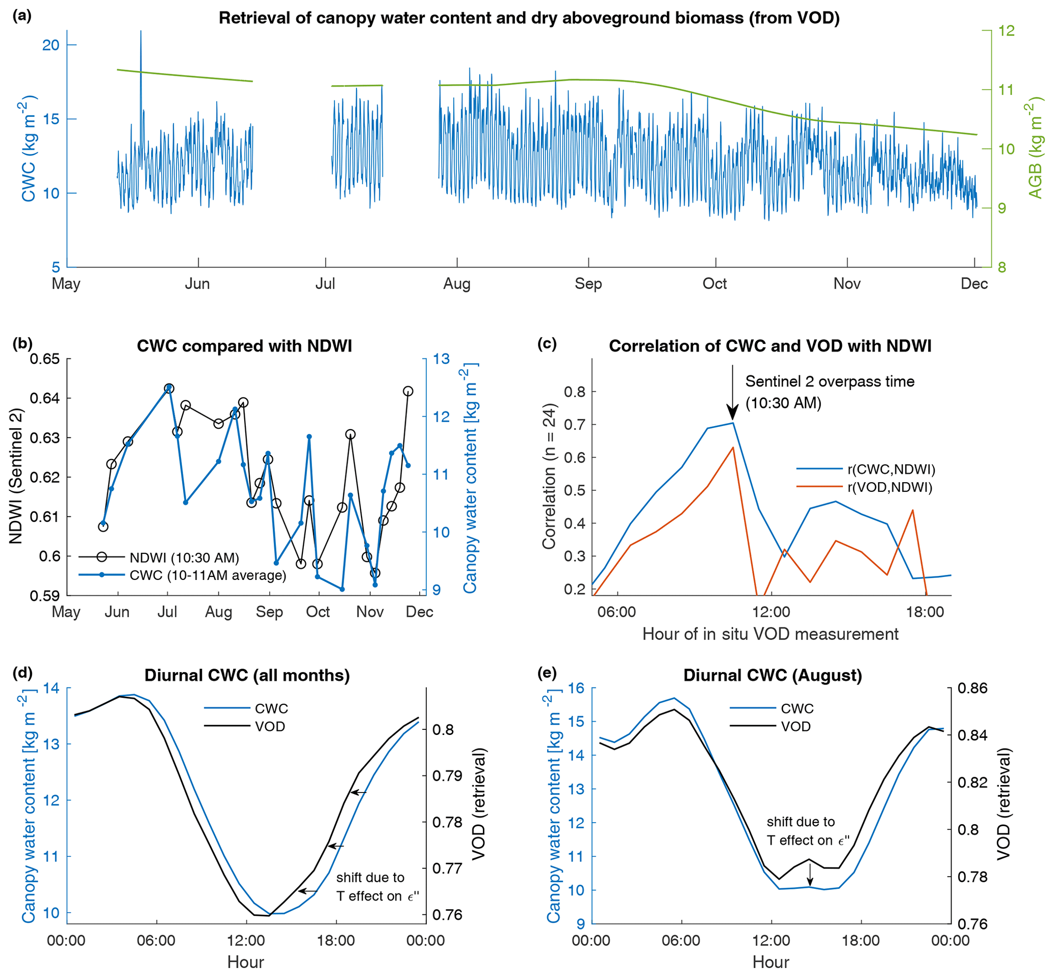
Figure 12 (a) Retrieval of canopy water content (CWC) and dry aboveground biomass (AGB). (b) Comparison between NDWI estimated from Sentinel-2 (HLS v1.4, 30 m resolution, https://hls.gsfc.nasa.gov/, last access: 20 April 2023) and our retrieval of CWC at the same hour as the Sentinel-2 overpass. (c) Correlation between Sentinel-2 NDWI and CWC or observed VOD at different hours of the day. (d) Long-term average diurnal cycle of CWC and modeled VOD (as predicted in Eq. 15). Panel (e) is the same as (d) but for the month of August only.

The diurnal dynamics of CWC are particularly strong, with a diurnal amplitude of 3.8 kg m⁻² on average, meaning that 28 % of the pre-dawn CWC is depleted over the course of the day (Fig. 12d). Such diurnal variations may seem important for a forested ecosystem but are not entirely inconsistent with other studies. Over a corn field in the Netherlands, Vermunt et al. (2022) observed that midday vegetation water content was decreased by 10%–20% on average compared to pre-dawn levels and even by 35.4 % on a particularly warm day. The results of Mirfenderesgi et al. (2016), who investigated the transpiration and sap flow dynamics of oaks in New Jersey with a hydrodynamic model, suggest a diurnal amplitude of about 15 % for just stem water storage. Matheny et al. (2017) also reconstructed a diurnal amplitude of 14.6 % to 22.3 % of the stem water storage from in situ sap flow measurements of red maple in Michigan. Since our estimate of CWC also likely incorporates an additional contribution from dew (discussed in the next section), an average CWC amplitude of 28 % would not be unexpected.

We find that our retrieval of CWC is slightly lagged compared to the diurnal average VOD cycle (Fig. 12d). This lag is due to the diurnal cycle of temperature and its effect on the dielectric loss (and thus on VOD), as represented in the dielectric model (Fig. 2b). The effect can also be seen in Fig. 12e, which focuses on the month of August. Here a minor peak in VOD can be observed at about 15:00 LT, in the center of the midday depression (also see Fig. 9a). Our retrieval suggests that at least some of this peak is in fact not related to rehydration but to a peak in diurnal temperature. In Fig. 13, we use the transmissivity model (Eq. 15) to explore the influence of moisture and temperature on modeled VOD (by enforcing a seasonally constant value for temperature and gravimetric moisture, respectively). As temperature increases during the day, it increases the dielectric loss and leads to a higher modeled VOD (Fig. 13a), thus counteracting the effect of moisture content changes to some extent. This effect was particularly pronounced during the heat wave that struck the area from 5 to 6 September (Fig. 13b). Here it can be seen that there is relatively little response in terms of VOD during the heat wave, with only a minor increase on 5 September. Because it is taking the response of the dielectric loss to temperature into account, the retrieval algorithm compensates for the effect of temperature with a marked CWC drop over that period (e.g., Fig. 12a), which makes sense from a physiological standpoint. Indeed, the record-breaking heat wave was accompanied by VPD values of up to 8 kPa on both days (compared to an average of 1 kPa the week before), and it would be very unlikely to see no response in CWC (and VOD) to such a level of stress.

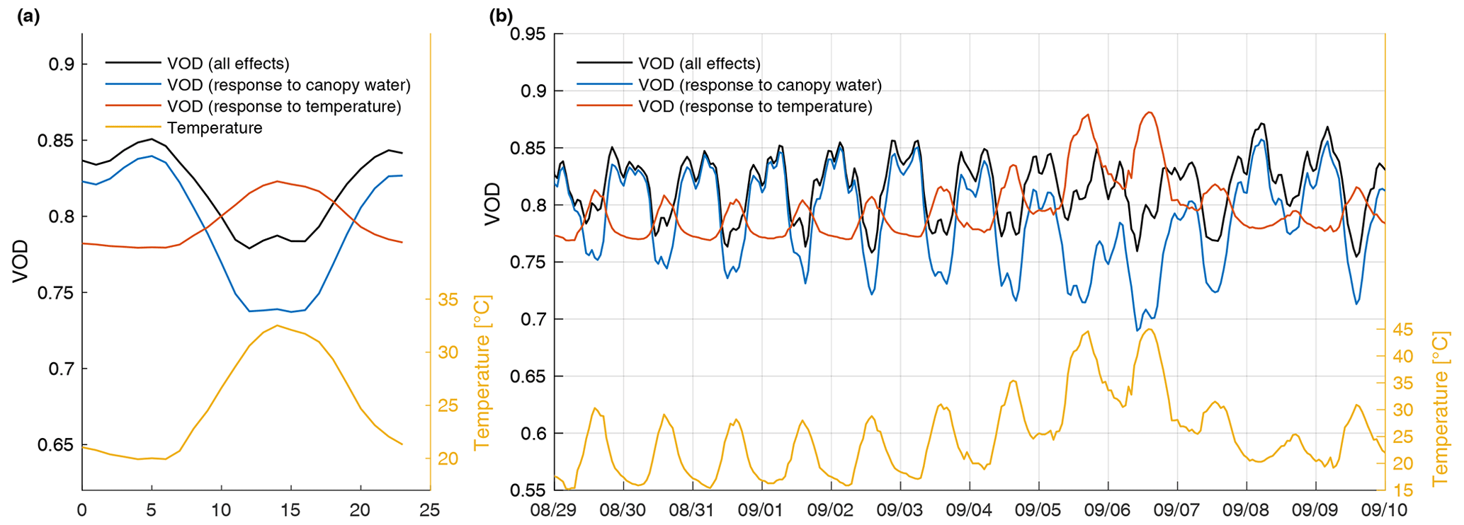
Figure 13 Counteracting effects of leaf gravimetric moisture and temperature on diurnal VOD changes, as predicted by the vegetation dielectric model of Ulaby and El-rayes (1987). (a) Modeled diurnal VOD response to leaf moisture and temperature averaged over the month of August. The VOD response to gravimetric moisture is estimated by setting temperature to its mean value in the model (and inversely for the response to temperature) (b) Modeled hourly VOD response to moisture and temperature in the context of the record-breaking heat wave of 5 to 6 September.

Figure 14 Surface canopy water effects. (a) VOD response to a rainfall event. The 5 min time series are smoothed with a LOESS filter (±1.5 h width). (b) Average diurnal CWC for nights with and without conditions favorable to dew deposition (solid versus dashed line). (c) Difference in CWC based on (b) compared against wetness sensor measurements (taken at the reference site).

This modeled response of VOD to high temperatures emerges directly from the dielectric model of Ulaby and El-rayes (1987). It is also predicted by another semi-empirical dielectric model of leaves proposed by Mätzler (1994), who confirmed such a temperature dependency with seasonal observations made in a beech forest (although they did not control for potential moisture changes as a covariate). It is very important to note that the magnitude and direction of the dielectric loss's dependence on temperature at L band are both dependent on the temperature itself (Fig. 2b). For instance, at temperatures between 0 and 20^∘ C the sensitivity of L-band VOD to temperature is negative (e.g., Schwank et al., 2021). We note that this temperature dependency can be quite crucial when interpreting water stress from VOD measurements. As water stress conditions often correlate with warm temperatures, one must be careful in interpreting VOD time series over a large dynamic range of canopy temperatures as using VOD alone might lead to unphysical interpretations, which in our case means an increase in canopy water in the middle of a heat wave.

4.3 Rainfall interception and dew

The only significant rainfall event during the measurement period occurred on 18 May (Fig. 14a). A cumulated precipitation amount of 10.2 mm was measured on that day and coincided with an increase in VOD of about 20 % compared to the usual diurnal cycle. Within a few hours following rainfall, this excess VOD quickly subsided but did not fully disappear until the day after. We could also establish that signal strength was likely not affected by the presence of intercepted water on the antenna itself (Fig. S2). These results indicate that L-band VOD is quite sensitive to intercepted rainfall, as has been shown with X-band VOD observations from the AMSR-E satellite (Xu et al., 2021) and from an in situ radiometer (Schneebeli et al., 2011). The VOD anomaly also lasted longer compared to the surface wetness measurements taken at the reference station (Fig. 14a). This is likely because the surface wetness instrument is exposed to sunlight and an open atmosphere, such that its surface water evaporates much faster compared to what happens in a forest canopy. If future research at eddy-covariance tower sites can demonstrate that such VOD measurements are a good proxy for intercepted water, this may provide a useful constraint to the partitioning of evapotranspiration fluxes into different sources (i.e., evaporation versus transpiration).

For completeness, we also investigate the effect of dew on our measurements in Fig. 14b–c. Unlike rainfall events, dew events have smaller impacts on VOD and are more difficult to isolate from other sources of variability. Thus, we focus on the retrieved CWC time series, as it is less influenced by day-to-day variability in temperature compared to the VOD measurements (as discussed in the previous section). To diagnose some possible effects of dew on CWC, we separate a 2-month observational subset into two samples based on the daily maximum relative humidity (RH_max). We use a threshold of 70 % relative humidity to distinguish nights with and without a potential for dew formation (Ritter et al., 2019). We then calculate the average diurnal CWC cycles for each of these two subsets (Fig. 14b) and compare their relative difference against the surface wetness measurements taken at the reference site (Fig. 14c). Because the surface wetness sensor tends to saturate relatively quickly, we exclude nights where the wetness sensor is stuck at its maximum value. While this does remove some nights where a lot of dew deposition is occurring, it has the advantage of preserving the proportionality between CWC and the wetness sensor measurements. We find a relatively good agreement between CWC and the wetness sensor data (Fig. 14c), suggesting that dew deposition is reflected in our CWC retrieval. This finding is of importance since dew deposition, even in southern California, would then influence and potentially bias calculated differences between midnight and midday satellite-based VOD, which have been used to interpret plant hydraulic behavior (Konings and Gentine, 2016). The two-peaked structure in Fig. 14c seems to be arising from the combination of individual dew accumulation events occurring either after sunset or before sunrise. It is important to note that because the transmissivity model does not represent surface water in a dedicated way (Schneebeli et al., 2011), the data in Fig. 14c should not be used to derive actual dew amounts. Here we can only conclude that L-band VOD is likely influenced by dew deposition, which is unlike Holtzman et al. (2021), who found no evidence for the impact of dew on VOD measurements in an oak forest, but in agreement with conclusions from several other studies (Xu et al., 2021;Schneebeli et al., 2011; Khabbazan et al., 2022).

5 Conclusions

In this paper we have demonstrated that a pair of GNSS receivers can be used to continuously measure L-band VOD in a forest stand. Thanks to the diversity of GNSS satellite orbits, a hemispheric scan of the canopy can be obtained, offering the opportunity to individually monitor specific trees, groups of trees, or classes of canopy density. While continuous changes in GNSS orbit patterns and constellation configurations complicate the analysis of raw observations, here we provide a relatively straightforward solution to alleviate this problem and produce credible VOD time series. Pooling observations from the four largest GNSS constellations (GPS, GLONASS, BeiDou, and Galileo), we show that VOD anomalies can be resolved at hourly resolution. In particular, our approach is able to identify a diurnal cycle in VOD that appears consistent with what has been reported in previous recent studies (Holtzman et al., 2021; Vermunt et al., 2021; Konings et al., 2017b). Here, obtaining such high-frequency (e.g., hourly) VOD time series comes at the cost of angular resolution, since measurements taken at all azimuths and elevation angles are aggregated into hourly averages. Because of the configuration of the GNSS orbits, users face a trade-off between obtaining VOD estimates at high angular resolution (e.g., Fig. 5b) versus obtaining VOD time series at high temporal resolution (e.g., Fig. 7b).

In a further step, we use existing simple models of canopy microwave transmissivity and vegetation dielectric parameters (Ulaby and Long, 2014) to demonstrate the feasibility of using such GNSS-based VOD observations to derive information about canopy water content and aboveground dry biomass (future work could certainly explore more complex formulations). Owing to the limited number of ancillary in situ measurements, this retrieval algorithm was not evaluated against long-term ground truth observations and should be seen as a proof of concept. Still, the resulting dry aboveground biomass and CWC estimates agree with what has been reported in similar studies. In addition, we show that the CWC estimates are in good agreement with satellite observations of the research site (NDWI from Sentinel-2), but this is only true if the hourly CWC estimates are taken precisely at the time of the Sentinel-2 overpass. This dependency of the agreement on the observation timing provides convincing and independent evidence that the CWC time series derived from GNSS-based VOD contains valuable information. We also investigate the potential effects of diurnal changes in temperature on the dielectric constant of the vegetation and its impact on L-band VOD and the retrieved CWC. We show that temperature effects on the vegetation dielectric at L band are predicted to play a minor but non-negligible role and can modulate VOD variability, especially for diurnal variability and during extreme events such as heat waves. Our results suggest that diurnal variability in VOD due to water content could be dampened and in some cases even reverted by the variability in temperature. This is because temperatures >20 ^∘C cause an increase in the dielectric loss in saline water, causing VOD to increase over the day, in a direction opposite to the expected effect of diurnal canopy dehydration. The magnitude of this temperature effect is dependent on the microwave frequency and the ionic conductivity of the plant water according to the empirical model of Ulaby and El-rayes (1987). Finally, we provide some evidence that GNSS-based VOD is sensitive to surface canopy water, for the cases of both rainfall interception and dew deposition.

Future work may focus on various aspects. Future deployments of GNSS-based measuring systems like the one proposed here will be made at heavily monitored ecohydrological research sites in order to facilitate cross-comparisons with other in situ data. At the time of writing, we have recently equipped three forested FluxNet eddy-covariance sites with pairs of GNSS sensors, one in the US (US-MOz) and two in Switzerland (CH-Lae and CH-Dav). Based on these new deployments, we provide below a few recommendations. The total cost to equip an existing research site was of about USD 2000, with two-thirds of that amount dedicated to acquiring the scientific instruments. The reference instrument may be placed at the top of a flux tower or at some other close location (i.e., <5 km away) with the clearest possible view of the sky. Positioning the subcanopy antenna is not subject to strong restrictions. It can even be placed on the ground (without a tripod) as long as it is level and free from obstructions. We suggest placing the antenna in direct view of frequently monitored trees and not too close to strong reflectors (large tree trunks, buildings). The sampling characteristics discussed in Sect. 2.6 and reported in Fig. 6a may be helpful in guiding new installations. Over flat terrain, the maximum extent of the observation footprint is dependent on the height of the vegetation (minus the subcanopy antenna height). Assuming that measurements with an elevation angle lower than 10^∘ are discarded, the footprint may be roughly estimated as a circle with a radius of $r=h/\text{tan}\left(\mathrm{10}{}^{\circ }\right)$, i.e., r≈57 m for h=10 m. We provide further recommendations in Table S1 in the Supplement. Other future objectives should include an evaluation of GNSS-based VOD estimates against other VOD measurements made by a tower-mounted radar or radiometer. In particular, the degree to which GNSS-VOD at RHCP-polarization agrees with other VOD estimates at horizontal (H) or vertical (V) polarization is unknown. For instance, previous studies over forests have shown that H-polarized VOD can differ from V-polarized VOD, even though temporal dynamics are similar (Schwank et al., 2021; Guglielmetti et al., 2008; Kurum et al., 2009b). Even though our observations do not suggest it, we cannot yet exclude the possibility that GNSS-based VOD has some type of bias compared to these other types of measurements (which do not constitute a reference per se). The question of how to best process the GNSS data in order to obtain VOD time series also remains to be explored. The initial solution provided in Sect. 2.6 may likely be refined to further reduce some of the noise still present in sub-hourly GNSS-based VOD time series. Some additional information may also be gained by using GNSS signals at multiple frequencies (here we used the most common signal, which is emitted at around 1.57 GHz, but individual constellations also broadcast signals at lower frequencies up to 1.17 GHz).

The results presented here suggest that GNSS-VOD may have the potential to fill a key research gap in terms of linking satellite-based L-band VOD observations to ground observations. This contribution could take place in several ways. For example, arrays of GNSS receivers deployed within the spatial footprint of a satellite VOD grid cell (i.e., about 30 km) may serve to estimate a regional average VOD that would be suitable as ground truth for the satellite products. In addition, long-term in situ VOD observations performed at existing ecohydrological research sites may serve to develop and evaluate retrieval algorithms that aim to transform VOD into other relevant quantities of interest like aboveground biomass, canopy water content, or leaf water potential. To the benefit of these research sites, GNSS-VOD provides a useful proxy to upscale and gap-fill time series of the time-consuming and labor-intensive measurements of leaf water status and biomass. The ability to detect rainfall interception and dew deposition at the scale of a whole canopy may also provide some key information to improve our understanding of water, energy, and carbon fluxes at these sites. While GNSS-based monitoring of the Earth system remains a relatively diverse and emerging research field, remote sensing of GNSS-VOD appears to be a particularly promising application because of its ability to address a series of research objectives at a modest cost.