Global analysis of the controls on seawater dimethylsulfide spatial variability

Dimethylsulfide (DMS) emitted from the ocean makes a significant global contribution to natural marine aerosol and cloud condensation nuclei and, therefore, our planet's climate. Oceanic DMS concentrations show large spatiotemporal variability, but observations are sparse, so products describing global DMS distribution rely on interpolation or modelling. Understanding the mechanisms driving DMS variability, especially at local scales, is required to reduce uncertainty in large-scale DMS estimates. We present a study of mesoscale and submesoscale (< 100 km) seawater DMS variability that takes advantage of the recent expansion in high-frequency seawater DMS observations and uses all available data to investigate the typical distances over which DMS varies in all major ocean basins. These DMS spatial variability length scales (VLSs) are uncorrelated with DMS concentrations. The DMS concentrations and VLSs can therefore be used separately to help identify mechanisms underpinning DMS variability. When data are grouped by sampling campaigns, almost 80 % of the DMS VLS can be explained using the VLSs of sea surface height anomalies, density, and chlorophyll a. Our global analysis suggests that both physical and biogeochemical processes play an equally important role in controlling DMS variability, which is in contrast with previous results based on data from the low to mid-latitudes. The explanatory power of sea surface height anomalies indicates the importance of mesoscale eddies in driving DMS variability, previously unrecognised at a global scale and in agreement with recent regional studies. DMS VLS differs regionally, including surprisingly high-frequency variability in low-latitude waters. Our results independently confirm that relationships used in the literature to parameterise DMS at large scales appear to be considering the right variables. However, regional DMS VLS contrasts highlight that important driving mechanisms remain elusive. The role of submesoscale features should be resolved or accounted for in DMS process models and parameterisations. Future attempts to map DMS distributions should consider the length scale of variability.

1 Introduction

Dimethylsulfide (DMS) is a volatile sulfur gas produced by surface ocean microbial food webs and emitted to the atmosphere (Bates et al., 1992). DMS emissions dominate atmospheric biogenic sulfur and form a significant component of natural marine aerosol loads (Simó, 2001; Sanchez et al., 2018; Quinn et al., 2017). Aerosols increase light scattering and modify cloud optical properties, thereby contributing to a radiative forcing of climate (Charlson et al., 1987; Carslaw et al., 2013; Galí et al., 2021). The amount, composition, and distribution of natural aerosol in the atmosphere determine the indirect radiative forcing effect of anthropogenic aerosols on climate, but these are poorly constrained by global climate models (Carslaw et al., 2013). DMS-derived sulfate aerosols are ephemeral (∼ 1 d residence time; Boucher et al., 2003) and of greater consequence for cloud modulation in remote pristine regions (Halloran et al., 2010). The distribution of natural marine aerosol sources should be represented at the resolution required to capture the frequency and magnitude of their variability. This is critical for reducing the large uncertainties associated with natural aerosol–cloud interactions.

Oceanic DMS production and consumption pathways are complex, and the controls on DMS spatial distribution in the global ocean are not fully resolved (Galí and Simó, 2015). The Global Surface Seawater DMS Database (GSSDD) contains measurements that show large-scale temporal and spatial variability in DMS concentrations (Lana et al., 2011; Hulswar et al., 2022). In situ DMS measurements are relatively sparse and limited with respect to global distribution, coverage, and spatiotemporal sampling frequency, rendering the majority of DMS observations insufficient to resolve local and submesoscale variability (Tortell et al., 2011; Belviso et al., 2004a; Lana et al., 2011). DMS sampling is globally biased towards spring–summer months (see Fig. S1, Supplement) and has disproportionally targeted biologically productive areas (e.g. northeastern Pacific and northwestern Atlantic, see Fig. 1), which can lead to an overrepresentation of high DMS concentrations within the database (Galí et al., 2018). Monthly and repeat interannual DMS measurements are rare and generally restricted to DMS productive areas (Galí et al., 2018; Tesdal et al., 2015). Sparse, infrequent, and seasonally and spatially biased observations of highly variable DMS concentrations create uncertainty because it is hard to quantify the representativeness of the measurements. Sampling uncertainties inevitably propagate through to DMS concentration and flux climatologies, parameterisations, and model outputs (Belviso et al., 2004b).

Figure 1 Global extent of the 37 high-frequency DMS campaigns included in this analysis (coloured). Data are only shown for the underway transects used in the VLS analysis (see Sect. 2.3). Insets show detail for northeastern Pacific and northwestern Atlantic regions with multiple sampling campaigns (see Table S2 and Fig. S1 in the Supplement for metadata relating to each sampling campaign and the spatiotemporal distribution, respectively).

Relatively simple extrapolation methods have been used to fill the gaps between sparse observations to provide globally representative estimates of DMS (Lana et al., 2011; Kettle et al., 1999; Hulswar et al., 2022). Significant differences in these smoothed climatological estimates, and thus uncertainties, have been attributed to the gap-filling techniques used, specifically the appropriate interpolation/smoothing radius of influence (Hulswar et al., 2022). More complex algorithms have been generated at the basin or global scale using parameters such as chlorophyll, light, nutrients, surface temperature, and mixed layer depth (Simó and Dachs, 2002; Anderson et al., 2001; Aranami and Tsunogai, 2004; Halloran et al., 2010; Vallina and Simó, 2007; Aumont et al., 2002; Belviso et al., 2004a; Galí et al., 2015, 2018; Miles et al., 2009; Chu et al., 2003; Herr et al., 2019). More recently, global and regional climatologies have been generated using machine learning approaches (Wang et al., 2020; McNabb and Tortell, 2023, 2022; Humphries et al., 2012). The variation in different climatological DMS estimates highlights that the scientific community needs to better understand and map the processes controlling its oceanic distribution (Halloran et al., 2010; Belviso et al., 2004b). Modelled seasonal and regional aerosol–cloud interactions and radiative forcing are directly sensitive to the accuracy and choice of seawater DMS estimates (Woodhouse et al., 2013, 2010; Mahajan et al., 2015).

Recent studies have focussed on local and submesoscale DMS variability, taking advantage of improvements to seawater DMS concentration sampling resolution (e.g. Asher et al., 2011; Nemcek et al., 2008; Tortell, 2005a, b; Tortell and Long, 2009; Zindler et al., 2014). This study explores the potential mechanisms that appear to govern DMS variability at the < 100 km scale and investigates whether these align with the variables used within large-scale DMS parameterisations. An improved understanding of submesoscale DMS variability will aid the development of future climatological flux estimates and the appropriate radius of influence that sparse observations should be afforded when smoothing and interpolating in situ observations.

Variability length scale (VLS) analysis is a powerful tool for quantifying submesoscale variability. VLS analysis can be used to indicate the lowest sampling resolution necessary to capture most of the spatial variability (Royer et al., 2015). High-resolution measurements are required to assess small-scale variability. For example, observing variations within 10 km when the research ship is travelling at 8 m s⁻¹ requires measurements every 20 min. Instruments that can observe variability at these high resolutions have been deployed in recent years and have substantially contributed to the global DMS database (Hulswar et al., 2022). A growing number of high-frequency DMS measurements offers the opportunity for a global analysis of the drivers of DMS variability at small scales.

VLS analysis for DMS has been applied in only a few studies, with most focusing on a specific region and/or a single sampling campaign (e.g. Ross Sea, Tortell and Long, 2009; Tortell et al., 2011; northeastern subarctic Pacific, Tortell, 2005b; Asher et al., 2011; Nemcek et al., 2008). A larger-scale VLS analysis was undertaken on the 7-month low- to mid-latitude global circumnavigation conducted during the Malaspina Expedition 2010 (M10; Royer et al., 2015). Royer et al. (2015) combined their VLS analysis with VLS values from three high-latitude studies (7–15 km; Asher et al., 2011; Nemcek et al., 2008; Tortell et al., 2011) and reported an inverse relationship between DMS VLS and latitude (R = −0.74, p < 0.005). Royer et al. (2015) also reported that biological variables dominate over physical variables as drivers of DMS VLS in low-latitude regions. While it is tempting to draw global conclusions from the similarities and differences between these studies, each study adopts a slightly different approach to the data treatment, measurement of interpolation error, and/or classification of VLS (see Table S1, Supplement).

This study applies a single, objective VLS analysis to high-frequency global DMS observations over the past 15 years (Figs. 1 and S1, Supplement). The dataset used includes all available data from previous VLS studies. Our study assesses whether the factors controlling DMS variability can be identified using a submesoscale variability analysis across all ocean basins. Section 2 describes the datasets used and the VLS methodology. Section 3 presents results including global VLS statistics, regional patterns of DMS variability, and drivers of DMS variability. Finally, the findings are discussed in Sect. 4, with conclusions made in Sect. 5.

2 Data and methods

2.1 Seawater DMS data

The majority of DMS data are sourced from the global surface seawater DMS database (GSSDD; see https://saga.pmel.noaa.gov/dms/, last access: 15 April 2022). Selection criteria are used to identify datasets suitable for submesoscale VLS analysis: a minimum of 100 data points in total and ≤ 1 h between measurements, which excludes all data with a spatial resolution of > 30 km. Applying these filters results in 37 eligible datasets (collected between 2004 and 2019). The filters broadly separate the DMS database by sampling method, highlighting the rapid shift during the early 2000s from discrete, low-frequency gas chromatography analytical systems to continuous, semi-automated high-frequency mass spectrometry (Bell et al., 2012; Saltzman et al., 2009). Additional data are from the Malaspina Expedition in 2010–2011 (M10; Royer et al., 2015), the North Atlantic Aerosol and Marine Ecosystem Study in 2015–2018 (NAAMES; Bell et al., 2021; Figs. 1 and S1, Table S2, Supplement, campaign numbers: 33 – blue, 34 – green, 35 – red, 36 – yellow), and the Southern oCean SeAsonaL Experiment in 2019 (SCALE; Manville and Bell, 2023​​​​​​​; Figs. 1 and S1, Table S2, Supplement, campaign number: 37, green). The M10 circumnavigation data are split spatiotemporally into three datasets, each broadly covering different ocean basins (Figs. 1 and S1, Table S2, Supplement, campaign numbers: 30 – M10a, black; 31 – M10b, dark red; 32 – M10c, cyan).

2.2 Ancillary in situ and coincident satellite measurements

Ancillary in situ and remotely sensed data are used to explore the potential mechanisms driving DMS variability. In situ sea surface salinity (hereafter salinity) and sea surface temperature (SST) from each DMS dataset are used to derive sea surface density (hereafter density) (see Fernandes, 2014).

Satellite monthly mean chlorophyll a (Chl) and 5 d sea surface height anomaly (SSHA) data are matched to the average date of each DMS sampling cruise. Satellite data pixels are extracted along the coordinates of the DMS cruise track using the NASA SeaDAS software (version 7.5.3). NASA MEaSUREs level 4 (L4) 0.17^∘ 5 d SSHA data are used to explore the role of eddies in driving DMS variability (Zlotnicki et al., 2019). NASA MODIS-Aqua level 3 (L3) 4 km monthly Chl is used as a proxy for plankton biomass and biological productivity (NASA Goddard Space Flight Center, 2018).

2.3 Data processing

Underway data are screened to only include data acquired when the ship speed was > 1 m s⁻¹ to avoid measurements made when ships were sampling on station. Ship speed is calculated from distance and time between measurements. Each DMS dataset and all its ancillary data are divided into transects. Transects are defined as continuous data sections with a minimum sampling frequency of 1 h. Most observations (83 %) captured by the temporal filter are < 2.2 km apart. The minimum transect length is calculated in two stages: (1) the linear distance between the start and end of a continuous data section must be > 100 km to avoid campaigns that targeted a specific area multiple times (e.g. a productive bloom or mesoscale eddy); (2) each dataset is divided into equal length transects, with an along-track distance of at least 100 km. The initial data processing yields 1039 continuous transects from 37 DMS campaigns, with each transect 100–199 km in cumulative length (Fig. 1).

2.4 Variability length scale (VLS) analysis

Previous DMS VLS studies have not applied a standardised or consistent approach (Royer et al., 2015; Asher et al., 2011; Tortell et al., 2011; Tortell, 2005b; Tortell and Long, 2009; Nemcek et al., 2008). The analysis presented here adopts the method used to study the VLS of seawater CO₂ (Hales and Takahashi, 2004), which was later applied to DMS by Tortell et al. (2011) and Nemcek et al. (2008).

The highest observational DMS sampling resolution in the datasets is typically between 0.2 and 2.2 km. Each data transect is subsampled repeatedly, starting from the first data point, at increasingly coarse spacings ranging from 2.2 km to half the length of the transect (the lowest possible resolution), increasing in 0.2 km increments. At each subsampling resolution, the first and last subsampled points of the data transect define the subsampling window. Subsampled data across the subsampling window are linearly interpolated to the resolution of the original data. Where the subsampling window matches the length of the data transect, the interpolation error associated with the subsampling resolution is calculated as the root mean squared error (RMSE) between the original and the interpolated values. Where the subsampling window is not equal to the length of the transect, the window is shifted along the transect, incrementing by one data point, and the transect is re-subsampled. Re-subsampled data are linearly interpolated across the shifted window, and the RMSE is re-calculated. The subsampling window is repeatedly shifted along the data transect and interpolation RMSE re-calculated until the subsampling ends on the last data point of the transect. The error associated with the subsampling resolution is taken as the average of all the RMSE values produced by sliding the window across the data transect at that resolution. The RMSE is calculated following Eq. (1):

$$\begin{array}{}\text{(1)}& \text{RMSE}=\sqrt{\stackrel{\mathrm{‾}}{(\text{Obs}-\text{Interp}{)}^{\mathrm{2}}}}.\end{array}$$

The RMSE typically increases in proportion to the coarseness of the subsampling until a maximum error plateau, or asymptote, is reached. The maximum error plateau corresponds to the total variance of the dataset (Tortell et al., 2011; Belviso et al., 2004a). The trend in RMSE as a function of subsampling resolution is well described by a non-linear first-order inverse exponential rise function following Eq. (2):

$$\begin{array}{}\text{(2)}& E_x=E_{\mathrm{\infty }}\left(\mathrm{1}-e^{\left(-\frac{x}{\text{VLS}}\right)}\right),\end{array}$$

where E_x is the interpolation error at subsampling resolution x, E_∞ is the asymptotic maximum interpolation error at an infinite subsampling resolution, and VLS is the characteristic length scale of variability. The VLS is determined by the subsampling resolution (interpolation distance) where a tangent of the initial slope intersects with the maximum error (E_∞, Fig. 2). The VLS also corresponds to the intersect on the curve (E_x) that is 63 % of E_∞, i.e. Eq. (3):

$$\begin{array}{}\text{(3)}& {\displaystyle \frac{E_x}{E_{\mathrm{\infty }}}}=\mathrm{1}-e^{\left(-\frac{x}{\text{VLS}}\right)}\approx \mathrm{0.63}.\end{array}$$

Previous work suggested that a sudden change (or “breakpoint”) in the RMSE slope can be used to characterise the DMS VLS (Royer et al., 2015; Asher et al., 2011). However, this approach is unreliable because the data assessed in this study show that the breakpoint does not always occur, and its identification is subjective (see Table S1, Supplement).

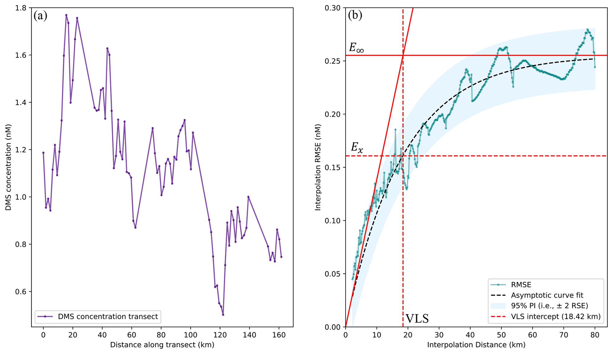
Figure 2 (a) Example of seawater DMS concentration (nM) data transect (sampled from the northwestern Atlantic during the NAAMES1 (November 2015) campaign; see Bell et al., 2021), analysed to find the variability length scale (VLS). (b) Asymptotic error curve (dashed black) fitted to interpolation errors (RMSE, nM; dotted cyan) plotted as a function of increasingly coarse interpolation distance (km). The 95 % prediction intervals (PIs) of the non-linear regression fit, i.e. $\pm \mathrm{2}\times$ residual standard errors (RSE), are shaded blue. The VLS (km) is characterised as the intercept (dashed red) on the curve at 63 % of the asymptotically approached maximum interpolation error (nM). Method adapted from Hales and Takahashi (2004).

An inverse exponential rise function (Eqs. 2 and 3) is used here to objectively derive the VLS. The objective VLS method is applied to all 1039 transects and six variables: DMS, SST, salinity, density, Chl, and SSHA.

2.5 Quality assurance and VLS statistics

Two filters are used to identify viable data transects. The VLS is rejected if the distance is greater than the maximum subsampling/interpolation distance (equal to half the transect length), which only occurred in very noisy datasets. The second filter is the quality of fit to the data using the residual standard error (RSE) (Fig. 2b), which is defined as RSE $=\sqrt{({\text{ss}}_{\text{res}}/n)}$, where n is the number of data points in the transect and ss_res is the sum of the squares of the residuals, i.e. ${\text{ss}}_{\text{res}}=\sum (\text{residuals from fitted curve}{)}^{\mathrm{2}}$.

The RSE is normalised using the maximum RSE of the curve (i.e. (RSE $/$ RSE at the asymptote) × 100), and if the normalised RSE exceeds 10 %, the curve is deemed to inadequately describe the data and the transect is rejected. The two quality control filters reduce the initial 1039 transects to 763 “viable” transects.

The VLS distributions from the 763 transects are skewed for all parameters (Figs. 3 and S2, Supplement). The geometric mean and geometric standard deviation (GSD) are computed to assess central tendency and spread while accounting for skew in the data. Note that the geometric mean is regularly referred to as the “average” within this paper to aid readability. All significance testing uses the non-parametric Mann–Whitney U test. Transects are grouped and averaged by sampling campaign to assess underlying spatial and temporal (regional and seasonal) patterns of variability. Average VLS distances are calculated for each sampling campaign and for all variables (VLS_DMS, VLS_SST, VLS_salinity, VLS_density, VLS_Chl, VLS_SSHA). A minimum threshold of four transects was necessary before calculating a campaign-averaged VLS. Exclusion of campaigns with fewer than four transects reduced the total number of campaigns from 37 to 35.

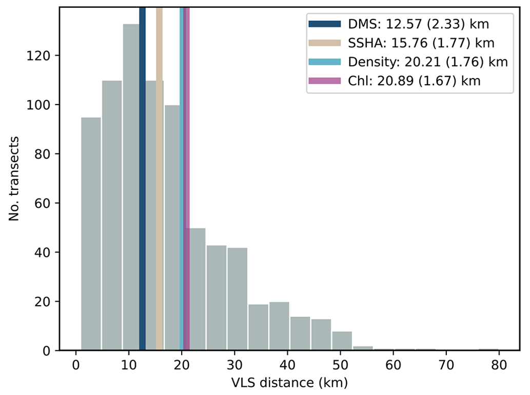
Figure 3 Frequency distribution of variability length scales (VLSs, km) for all DMS transects (grey bars). Vertical coloured lines correspond to the global geometric mean (and geometric standard deviation, GSD) from all transects for VLS_DMS (dark blue), VLS_SSHA (beige), VLS_density (cyan), and VLS_Chl (magenta).

Correlation and multiple linear regression (MLR) are used to explore the global controls on VLS_DMS (see Sect. 3.3.1 and 3.3.2). The campaign-averaged VLS used in each correlation and regression analysis only includes transects where coincident VLS can be calculated from the DMS and non-DMS variables. The MLR models with two input variables contain 20–26 datasets, and MLR models with three input variables contain 11–15 datasets. The relative importance of the input variables in each MLR model are calculated based on the incremental R² used to determine interactional dominance (defined as the incremental R² contribution of each predictor to the complete model; Azen and Budescu, 2003).

3 Results

3.1 Global VLS statistics

The global average DMS concentration and geometric standard deviation (GSD) for the viable transects covered in this study are 2.23 nM (average) and 2.29 (GSD), which are similar to the global average and GSD from the GSSDD (2.66 nM (average), 2.88 (GSD); https://saga.pmel.noaa.gov/dms/, last access​​​​​​​: 15 April 2022). The similarity between the two datasets suggests that the data used in this study are representative of global observations. The global average and GSD of VLS_DMS from all 763 transects are 12.57 km and 2.33, respectively (Fig. 3). The global average VLS_DMS is the smallest of the six variables tested, with VLS_SSHA the most similar (15.76 km, 1.77 GSD) (Fig. 3). Global average VLS_Chl is slightly larger (20.89 km, 1.67 GSD) and similar to global average VLS_density (20.21 km, 1.76 GSD) and its components VLS_SST (21.23 km, 1.73 GSD) and VLS_salinity (19.52 km, 1.84 GSD) (Figs. 3 and S1, Supplement). Global average VLS_DMS and VLS_SSHA are significantly different (p < 0.01) from each other and the global average VLS of all other parameters. Global average VLS_Chl, VLS_density, VLS_SST, and VLS_salinity are not significantly different from one another.

All six variables have an average spatial variability that is tens of kilometres in all regions. The global average VLS_SSHA is similar (within 4 km) to the global average VLS_DMS. The global average VLSs for all other parameters are within 9 km of the global average VLS_DMS. The campaign-averaged VLS_DMS ranges from 2 to 30 km, which is the same order of magnitude as the range of 7–50 km reported by other DMS variability studies (Asher et al., 2011; Nemcek et al., 2008; Tortell, 2005b; Tortell et al., 2011; Royer et al., 2015). Note that a detailed comparison between studies should be treated with caution because each has used different methods to identify the VLS.

3.2 Regional patterns of DMS variability

VLS_DMS is generally small in the subtropical gyres, specifically the equatorial and subtropical South Pacific and South Atlantic (Fig. 4; see Table S2, Supplement, for the campaign-averaged VLS_DMS of each sampling campaign, e.g. campaign numbers: 30, M10a, black; 31, M10b, dark red; and 32, M10c, cyan). The average VLS_DMS from all transects in the three M10 low- to mid-latitude circumnavigation campaign datasets (mean = 6.34 km, GSD = 2.59) is consistently smaller than the global value (mean = 12.57 km, GSD = 2.33) (Fig. 4). The relative homogeneity of small VLS_DMS in these oligotrophic domains is not replicated in the VLS of any other variables (Fig. S3, Supplement). The subtropical gyres of the Southern Hemisphere are permanently stratified biomes, bounded to the south by a band of seasonally stratified biomes (Fay and McKinley, 2014). At the boundary transitions from permanently to seasonally stratified conditions, there are some notable exceptions to the low VLS_DMS, e.g. the Benguela upwelling (southeast Atlantic) and South Australia upwelling (Fig. 4).

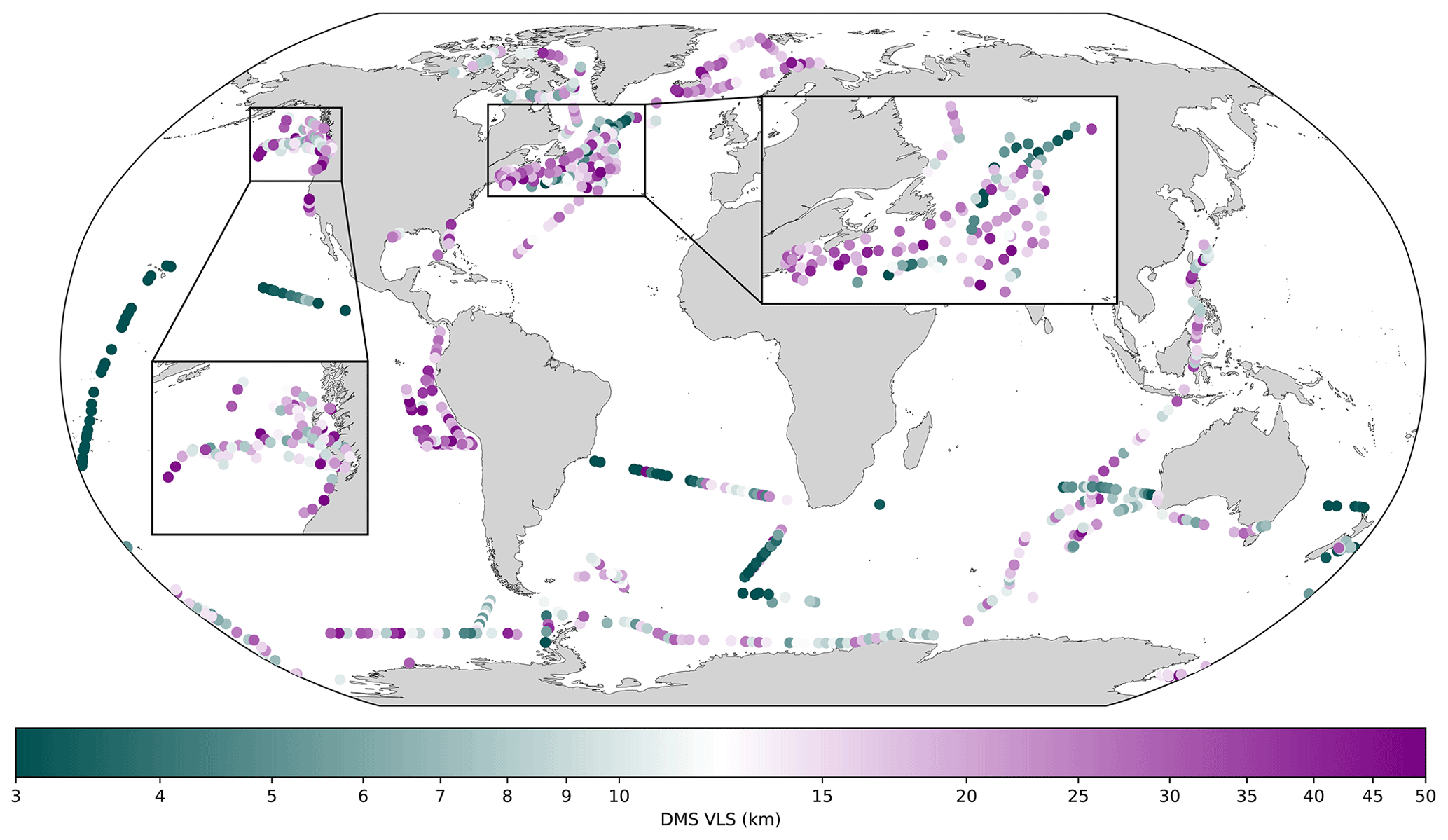
Figure 4 Global distribution of 763 transects coloured by VLS_DMS (km, log scale). The colour bar diverges at the global geometric mean VLS_DMS (12.57 km). See Fig. S3 in the Supplement for equivalent VLS distribution maps of Chl, density, SSHA, salinity, and SST and Fig. S1 for the spatiotemporal distribution of VLS_DMS.

In contrast, the average (mean = 22.06 km, GSD = 1.60) of VLS_DMS in the Peruvian upwelling (eastern equatorial Pacific) is consistently larger than the global average (mean = 12.57 km, GSD = 2.33) (Fig. 4). Larger VLS_DMS values are also found along parts of the Pacific and Atlantic coastlines of North America, with smaller VLS_DMS values further offshore (Fig. 4, inset). The VLS_DMS values in the Arctic, northeastern Pacific, northwestern Atlantic, and southeast Indian open ocean regions are highly variable. The Southern Ocean has VLS_DMS generally below the global average and features some localised pockets with larger VLS (Fig. 4). The DMS concentration variability in mid- to high-latitude regions is seasonal (Hulswar et al., 2022), and VLS_DMS could be influenced by the season/time of year.

3.3 Drivers of DMS variability

3.3.1 Transect and campaign-averaged VLS regressions

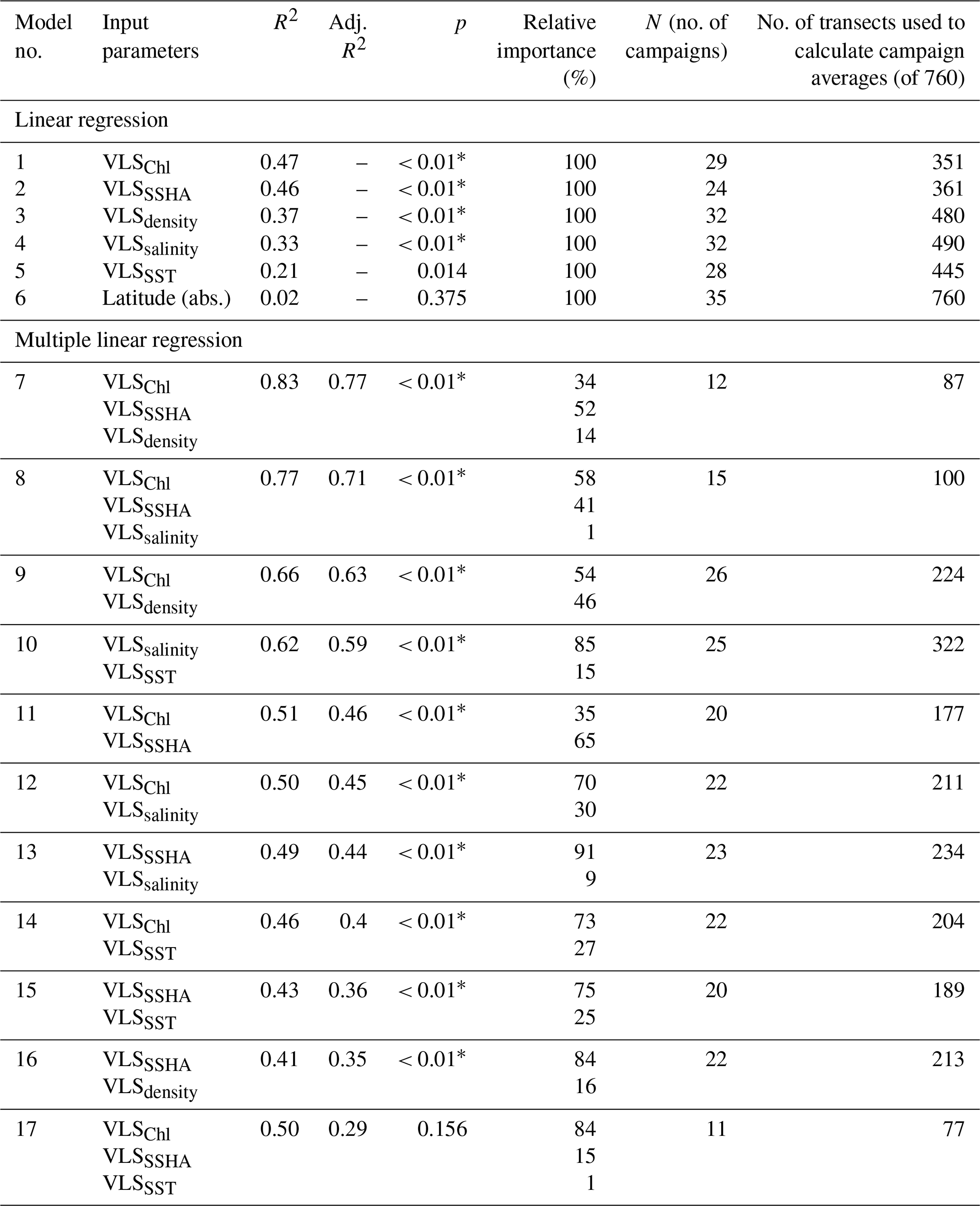
Simple linear regressions are used to explore the relationship between VLS_DMS and VLS for SST, salinity, density, Chl, and SSHA. The possibility of a relationship with latitude (as discussed in Royer et al., 2015) is also investigated. Transect and campaign-average VLS_DMS do not vary with latitude (R² = 0.02, n = 35, p > 0.05; Table 1). No significant relationships are observed between transect VLS_DMS and VLS for SST, SSS, density, Chl, and SSHA. Averaging transect VLS data into campaign averages reduces the noise and enables statistically significant relationships to be identified. The campaign-averaged VLS_density explains 37 % of the variations in VLS_DMS (Table 1; Fig. 5a); VLS_SSHA (used as an indicator of the dynamic eddy field in the open ocean) and VLS_Chl each explain approximately half of the campaign-averaged VLS_DMS (46 % and 47 %, respectively; Table 1; Fig. 5b and c).

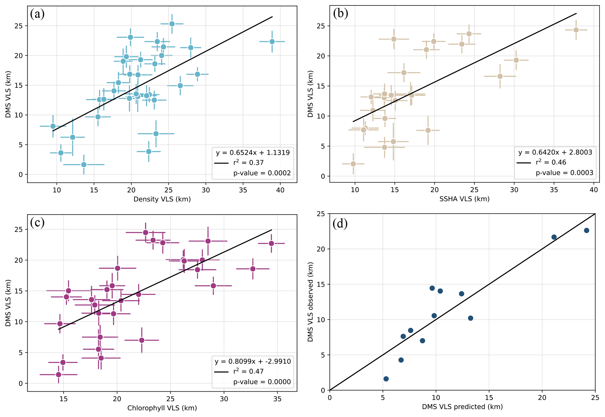
Figure 5 Campaign geometric mean VLS_DMS (km) plotted versus (a) VLS_density, (b) VLS_SSHA, and (c) VLS_Chl. Error bars indicate 1 GSD of the data within each campaign. (d) Campaign geometric mean VLS_DMS predicted using coefficients from the VLS_{SSHA–Chl–density} multiple linear regression model (Model 7, Table 1; Supplement, Table S4; Fig. S4) versus observed VLS_DMS for the subset of 12 DMS campaigns included in the multiple linear regression model. The 1 : 1 line is shown.

Table 1 Regression results for the prediction of campaign-averaged VLS_DMS, using different combinations of input parameters. Models are ranked in order of how much VLS_DMS variance is explained. Models that are significant (p < 0.01) are denoted using ^∗.

3.3.2 Multiple linear regression of VLS_DMS

Multiple linear regression (MLR) is used on the campaign-averaged VLS for SST, salinity, density, Chl, and SSHA to explore VLS_DMS variance (Table 1; see Table S4, Supplement, for regression coefficients). Eleven MLR combinations were tested, and all results are significant (p < 0.01), except for the combination of VLS_Chl, VLS_SSHA, and VLS_SST (Model 17, Table 1). Note that the number of available datasets is reduced in the MLR models that have more input variables, which results in the contribution of fewer data (campaigns) to the result. The number of input data is substantially increased if campaign averages are calculated without filtering the data prior to correlation, so they only contain data where the two or more correlated variables are co-located. Relaxing the criteria such that the transects need not be coincident increases the number of campaigns that can be included in each MLR model. The “relaxed criterion” approach is less robust but gives similar results to those presented here (see Table S3, Supplement).

Individual VLS_Chl and/or VLS_SSHA regressions with VLS_DMS are outperformed (i.e. R² > 0.47) by four MLR combinations (Models 7–10, Table 1). The combination of VLS_density and VLS_Chl (Model 9, Table 1) substantially improves the regression with VLS_DMS (adjusted R² increases to 0.63). MLR Model 9 has the most campaigns (n = 26) of any model and the third highest number of available data transects (n = 224); VLS_Chl (54 %) and VLS_density (46 %) make approximately equal contributions to the changes in VLS_DMS described by Model 9.

The largest amount of VLS_DMS variability explained by the MLR models uses the combination of VLS_SSHA, VLS_Chl, and VLS_density, improving the adjusted R² to 0.77 (Model 7, Table 1; Fig. 5d). The dominant parameter in Model 7 is VLS_SSHA (52 % of the explained variance), with VLS_Chl and VLS_density accounting for 34 % and 14 %, respectively. Combining VLS_Chl and VLS_SSHA (MLR Model 11) reduces the available input data (n = 20) and does not increase the explained variance in VLS_DMS compared to using only one or other of the input parameters. When paired with one other variable, VLS_SSHA and VLS_Chl dominate the explained variance in MLR models (Models 12–16, Table 1).

4 Discussion

4.1 Global statistics

This is the first study of submesoscale seawater DMS variability from a global perspective. Spatial variability length scale (VLS) analysis is applied to every ocean basin and at different times of year using a consistent methodology. Characteristic spatial variability in all six variables (DMS, SST, salinity, density, Chl, SSHA) occurs at the low mesoscale (in the tens of kilometres) in all regions. The campaign-averaged VLS_DMS ranges from 2–30 km (Table S2, Supplement); this is in general agreement with previous work (Royer et al., 2015; Nemcek et al., 2008; Asher et al., 2011; Tortell, 2005b; Tortell and Long, 2009; Tortell et al., 2011). There is no correlation between the campaign-averaged DMS concentration and VLS_DMS (R² = 0.01, p > 0.05), which suggests that understanding the variability may be a helpful and independent approach to understanding the processes that control surface ocean DMS.

4.2 Regional patterns of DMS variability

VLS_DMS is generally above average at the edge of ocean basins, e.g. parts of northwestern Atlantic, northeastern Pacific, and the California coast (Fig. 4, inset). It may be possible that the longer length scales of coastal DMS spatial variability are driven by large phytoplankton blooms, which previous local and regional studies suggest can dominate coastal domains (Asher et al., 2011; Nemcek et al., 2008). This work does not investigate the detail of drivers of DMS variability in individual regions or domains.

Open ocean domains such as the subtropical gyres in the Southern Hemisphere have generally small VLS_DMS, a feature not evident in the VLS of the other parameters (Figs. 4 and S2, Supplement). Short length scales of DMS variability in stable stratified biomes offer the opportunity for future work to re-examine these regions for as yet unidentified drivers of variability. Most low-latitude DMS data used in this study originate from a single sampling campaign (e.g. Malaspina Expedition 2010; Royer et al., 2015). To test if small VLS_DMS is a persistent feature in undersampled subtropical open oceans, more high-resolution observations are needed.

Factors driving temporal DMS variability are not explored in this study. However, complex VLS_DMS fluctuations at high latitudes (e.g. northwestern Atlantic, northeastern Pacific, Southern Ocean; Fig. 4) may be capturing variations in both space and time; VLS_DMS in high-latitude dynamic regions could be related to the seasonality of biological productivity and eddy activity (see Asher et al., 2011; Behrenfeld et al., 2019; Bell et al., 2021; Fox et al., 2020; Gaube et al., 2019; Herr et al., 2019; Lana et al., 2011; McGillicuddy, 2016). Additionally, it is plausible that VLS_DMS in the polar regions may be sensitive to the seasonal impact of sea ice on biogeochemical processes (see Galí et al., 2021; Lannuzel et al., 2020; Stefels et al., 2018). There are not enough repeat measurements made in high-latitude (high seasonal variability) regions to establish the impact of seasonality on VLS_DMS. In this study, the only region sampled during different seasons is the northwestern Atlantic (four Atlantic NAAMES campaigns; Bell et al., 2021), and there is not yet compelling evidence of a temporal difference between the VLS_DMS of these cruises/seasons. The VLS_DMS values of the NAAMES1 transects (November; average = 11.93 km, GSD = 1.76) are significantly different (p < 0.01) from the transect VLS_DMS of NAAMES3 (U = 99, p < 0.01; September; average = 20.89 km, GSD = 1.69) and NAAMES4 (U = 89, p < 0.01; March–April; average = 21.94 km, GSD = 1.57), but not from NAAMES2 (U = 108, p = 0.014; May–June; average = 18.4 km, GSD = 1.56). VLS_DMS values of the NAAMES2, 3, and 4 transects are not significantly different from each other (all p > 0.2).

4.3 Drivers of DMS variability

The variance in campaign-averaged VLS_DMS data explained by physical processes (represented by VLS_SSHA) is as important as biogeochemical processes (represented by VLS_Chl), with each parameter able to explain just under half of the VLS_DMS (Models 1 and 2, Table 1; Fig. 5). This conclusion contrasts with the findings of Royer et al. (2015), who find that the majority of VLS_DMS (65 %) in the low to mid-latitudes is more similar to the VLS of biological variables that represent biomass and physiology (Chl and fluorescence) than to the VLS of physical variables. These contrasting conclusions potentially reflect the fact that length scales of physical oceanographic variability increase towards the Equator due to the effects of the Earth's rotation. The Coriolis parameter and therefore Rossby radius are intrinsically latitudinally dependent (Jacobs et al., 2001). The longer transects used by Royer et al. (2015) at low to mid-latitudes enable them to capture scales of variability that may be associated with large physical features. This point is discussed further in in Sect. 4.5.

A larger proportion of campaign-averaged VLS_DMS variability (77 %) can be explained using VLS_Chl, VLS_SSHA, and VLS_density (Model 7, Table 1) compared to just VLS_SSHA or VLS_Chl. The data included in the VLS_{SSHA–Chl–density} MLR (Model 7, Table 1) are a subset but include at least one campaign from each major ocean basin (Fig. S4, Supplement) and thus represent a significant relationship with global applicability. VLS_SSHA explains the majority of VLS_DMS in the VLS_{SSHA–Chl–density} MLR (52 %) (Model 7, Table 1) and improves the prediction of changes in VLS_DMS compared to using just VLS_Chl and VLS_density (Model 9, Table 1). The VLS_{SSHA–Chl–density} MLR (Model 7, Table 1) includes measurements from the NAAMES4 (2018) cruise, which targeted a substantive eddy and observed a persistent high Chl feature coincident with elevated DMS levels (Bell et al., 2021). The water mass within an eddy tends to be retained by the circulation, such that plankton within the eddy are accumulated under relatively stable physics (upwelling or downwelling) and consistent biogeochemical conditions (Bell et al., 2021). Eddies may thus drive conditions where DMS variability is closely associated with biological activity and a clear covariation in VLS is observed, even if the relationship between DMS and Chl concentration is less obvious (della Penna and Gaube, 2019). The relationship between eddy structure, biogeochemistry, and DMS may explain the link between changes in VLS_DMS, VLS_SSHA, and VLS_Chl. The importance of VLS_SSHA for predicting VLS_DMS is consistent with results recently reported by McNabb and Tortell (2022), who apply two independent machine learning techniques to analyse DMS in the northeastern Pacific. McNabb and Tortell (2022) demonstrate the power of mesoscale eddies for predicting DMS variability (Spearman correlation coefficients = 0.35 and 0.42, depending on the machine learning method employed), using the same SSHA product used in this study (using only summertime measurements, 1997–2017). The VLS_{SSHA–Chl–density} MLR model coefficients (Model 7, Table S4, Supplement) are used to predict VLS_DMS for the target input data subset (Fig. 5d). The residuals of predicted VLS_DMS are not systematically biased within the full range of the data (5–25 km).

4.4 Implications for global DMS parameterisation

Low-resolution measurements have previously been used to predict mean spatiotemporal patterns of DMS, both regionally and globally. Several studies have parameterised DMS as a function of surface mixed layer depth (MLD), light, and Chl (Vallina and Simó, 2007; Galí et al., 2018; Simó and Dachs, 2002; Aumont et al., 2002; Anderson et al., 2001; Belviso et al., 2004a; Aranami and Tsunogai, 2004). For example, Simó and Dachs (2002) use climatological MLD and remotely sensed Chl to estimate average DMS concentrations, while Vallina and Simó (2007) use climatological MLD, surface irradiance, and light attenuation to estimate surface DMS from the “solar radiation dose”. Galí et al. (2018) employ an algorithm driven by climatological Argo MLD and satellite-derived Chl, SST, and photosynthetically active radiation (PAR). Only the latter algorithm was additionally validated at finer resolution using non-climatological data to enable regional time series studies (Galí et al., 2019). SSHA reflects surface mixing and changes to the MLD (Gaube et al., 2019). This study supports the choice of key variables used in existing empirical parameterisations by demonstrating that, even on small scales, physical mixing (SSHA, density) and biological activity (Chl) explain a large portion of surface seawater DMS spatial variability in the global ocean.

The DMS parameterisations with global coverage that rely on remote and autonomous observations predict spatially and seasonally averaged surface seawater DMS reasonably well (e.g. Galí et al., 2018; Simó and Dachs, 2002; Vallina and Simó, 2007). However, some studies have questioned whether such parameterisations are overly reliant on spatial and/or temporal averaging, often to 1^∘ and/or monthly resolution (e.g. Derevianko et al., 2009). The spatiotemporal averaging used to develop global parameterisations may lead to an overconfidence in current predictive capabilities because key parameters are not included. Statistically significant MLR relationships in this study are obtained once the transect data are averaged by campaign, and the average VLS for all six variables in our study is tens of kilometres. Using VLS analysis to assess the covariation of parameters at the submesoscale provides insights that can help to improve global parameterisations. Our results indicate that patterns of mesoscale and submesoscale DMS variability, particularly those associated with SSHA, will be obscured at the 1^∘ resolution of most global parameterisations, highlighting the importance of modelling work at finer resolutions (e.g. Galí et al., 2019; McNabb and Tortell, 2022, 2023). Regional studies have tested empirical predictive relationships for DMS with varying degrees of success (Asher et al., 2011; Royer et al., 2015; Bell et al., 2006, 2021).

4.5 Study limitations and unidentified drivers of DMS variability

This work provides as comprehensive an assessment of DMS variability across the global ocean as existing data allow; however, many regions have not yet been sampled at high enough resolution to permit an assessment of VLS_DMS. For example, only 7 of the 37 campaigns in this study have made high-resolution DMS measurements in low-latitude waters (30^∘ N–30^∘ S). There is a seasonal sampling bias within the DMS database, and the northwestern Atlantic is the only region to have been assessed for VLS throughout the seasonal cycle (Bell et al., 2021). More data are needed.

Satellite-derived VLS_Chl and VLS_SSHA have been used to predict VLS_DMS (e.g. Model 7, Table 1), but this relies on the assumption that the satellite-retrieved data are representative of phytoplankton productivity and eddy activity throughout the research cruise/campaign. Satellite retrievals for Chl with higher than monthly temporal resolution or, in the case of SSHA, higher than 0.17^∘ spatial resolution may improve the ability to explain variance in VLS_DMS.

Transect lengths between 100 and 199 km are used to ensure comparability between datasets/regions because VLS results from previous studies appear to be sensitive to the length of data transect (see Fig. S5, Supplement). However, by limiting the transect length, it is difficult to identify large eddies using VLS_SSHA. Eddy length scales are typically larger at low latitudes due to the dependence of the Coriolis parameter on latitude (Chelton et al., 1998). The maximum VLS in this study is between 50 and 99.5 km (half the transect length), which is long enough to capture the eddy variability at latitudes where the eddy length scale is related to the Rossby radius of deformation, i.e. poleward of 30^∘, where the deformation radius is < 30 km (Eden, 2007). Equatorward of 30^∘, eddy length scales are not well predicted by the Rossby radius of deformation and can exceed 50 km (Tulloch et al., 2011; Scott and Wang, 2005; Klocker et al., 2016; Eden, 2007; Rhines, 1975). The VLS_SSHA analysis approach used in this study is designed to identify the dominant scale of variability in physical features up to 50–99.5 km; therefore, it may not capture the full extent of variability associated with large eddies at low latitudes. Large eddies will, however, still be captured in the VLS_SSHA analysis where a transect segments an eddy without passing through its centre. We also note that although SSHA is used to represent eddy features, at the Equator, stratification and strong westward currents tend to dominate SSHA variability rather than rotation and eddy transport (Williams and Follows, 2011).

In the subtropical gyres, VLS_DMS is typically small (< 10 km; Fig. 4), which is qualitatively consistent with the short (days) response time of DMS to perturbations in the dynamic equilibrium of DMS production and consumption in these waters (Galí and Simó, 2015); VLS_DMS in subtropical waters does not correspond well with the VLS of any of the other parameters (Fig. S3, Supplement). Cycling of reduced sulfur compounds in subtropical waters is well documented to be part of a different biogeochemical regime compared to productive, higher-latitude waters (e.g. Galí and Simó, 2015; Toole and Siegel, 2004). In stable oligotrophic regions where there is less variability in physical mixing and phytoplankton productivity, VLS_DMS could thus be dominated by alternative parameters that drive variability in the biological cycling of DMS such as zooplankton grazing (Simó et al., 2018) and microbial organosulfur metabolism (Nowinski et al., 2019; Cui et al., 2015; Alcolombri et al., 2015).

The so-called “summer paradox” describes the seasonal misalignment between maximum concentrations of phytoplankton biomass and DMS in low-latitude waters, and it has been challenging to model (e.g. Galí and Simó, 2015; Polimene et al., 2012; Toole et al., 2008; Vallina et al., 2008). In these areas, characterised by low seasonal amplitude in phytoplankton biomass, changes in phytoplankton species succession and physiological stress control DMS production yields and rates and, ultimately, DMS seasonality. By contrast, aggregated loss processes exhibit low seasonal variability and are insufficient to explain large-scale DMS seasonality in summer paradox areas (Galí and Simó, 2015). Previous studies observed important short-term variations in the balance between DMS sources and sinks in oligotrophic waters, concomitant with meteorological forcing (Royer et al., 2016). Hence, it is plausible to hypothesise that subtle changes in this balance can explain some of the variance in VLS_DMS. Light exposure in surface waters influences plankton physiological production and stress, photochemical reactions, and bacterial activity and thus has a significant impact on the cycling of reduced sulfur in oligotrophic regions (see Toole and Siegel, 2004; Vallina et al., 2008). These factors have not been included in the present study.

5 Conclusions

This study presents a comprehensive and objective analysis of DMS variability based on a large global dataset of high-frequency observations at the local/regional scale. The work shows that the variability length scale for DMS is typically small (< 30 km) and that a substantial proportion of the campaign-averaged variance can be explained by the VLS of key biological (Chl) and physical (density, SSHA) observations (Model 7, Table 1). The results improve confidence in the validity of the biological and physical parameters used to currently parameterise seawater DMS at large scales and used in many global climate models (e.g. Bock et al., 2021; Galí et al., 2018; Mulcahy et al., 2020; Simó and Dachs, 2002). However, there is substantial variability in VLS_DMS when assessing individual transects, which suggests that unaccounted-for variables are also important (e.g. light, wind speed, microbial diversity and activity). Making high-frequency measurements of these parameters at the same time as high-frequency DMS measurements may help to elucidate their role in DMS cycling.