the Creative Commons Attribution 4.0 License.
the Creative Commons Attribution 4.0 License.
 | 13 Jun 2023
A process-based model for quantifying the effects of canal blocking on water table and CO2 emissions in tropical peatlands
Marjo Palviainen
Hannu Hökkä
Sebastian Persch
Jeffrey Chatellier
Ophelia Wang
Prasetya Mahardhitama
Rizaldy Yudhista
Annamari Laurén
Drainage in tropical peatlands increases CO2 emissions, the rate of subsidence, and the risk of forest fires. To a certain extent, these effects can be mitigated by raising the water table depth (WTD) using canal or ditch blocks. The performance of canal blocks in raising WTD is, however, poorly understood because the WTD monitoring data are limited and spatially concentrated around canals and canal blocks. This raises the following question: how effective are canal blocks in raising the WTD over large areas? In this work, we composed a process-based hydrological model to assess the peatland restoration performance of 168 canal blocks in a 22 000 ha peatland area in Sumatra, Indonesia. We simulated daily WTD over 1 year using an existing canal block setup and compared it to the situation without blocks. The study was performed across two contrasting weather scenarios representing dry (1997) and wet (2013) years. Our simulations revealed that, while canal blocks had a net positive impact on WTD rise, they lowered WTD in some areas, and the extent of their effect over 1 year was limited to a distance of about 600 m around the canals. We also show that canal blocks are most effective in peatlands with high hydraulic conductivity. Averaging over all modeled scenarios, blocks raised the annual mean WTD by only 1.5 cm. This value was similar in the dry (1.44 cm) and wet (1.57 cm) years, and there was a 2.13 fold difference between the scenarios with large and small hydraulic conductivities (2.05 cm versus 0.96 cm). Using a linear relationship between WTD and CO2 emissions, we estimated that, averaging over peat hydraulic properties, canal blocks prevented the emission of 1.07 Mg ha−1 CO2 in the dry year and 1.17 Mg ha−1 CO2 in the wet year. We believe that the modeling tools developed in this work could be adopted by local stakeholders aiming at a more effective and evidence-based approach to canal-block-based peatland restoration.
- Article
(5558 KB) - Full-text XML
- BibTeX
- EndNote


Tropical peatlands contain approximately one-sixth of the global soil carbon pool (Page et al., 2011, 2022; Xu et al., 2018). In the recent decades, extensive tropical peatland areas have been converted to agricultural and plantation forest production sites (Miettinen et al., 2016; Wijedasa et al., 2018). This land use change has often been driven by drainage, which involves excavating canals or ditches in the peat. Canals help to remove water from the naturally waterlogged peat, enhancing site productivity and opening pathways for wood and crop transportation (Dohong et al., 2017). However, the same mechanisms that make the drainage-based bioproduction economically valuable have severe environmental consequences. Drainage increases CO2 emissions (Novita et al., 2021; Jauhiainen et al., 2012; Ishikura et al., 2018; Carlson et al., 2015), the rate of peat subsidence (Evans et al., 2022, 2019; Hooijer et al., 2012; Sinclair et al., 2020; Hoyt et al., 2020), fire risk (Miettinen et al., 2017; Kiely et al., 2021), nutrient release (Laurén et al., 2021), and nutrient export to water courses, and it decreases the peat substrate quality (Könönen et al., 2018).
Drainage lowers the peatland water table depth (WTD – meters, negative downward), which activates mechanisms that are behind the environmental drawbacks. The lower WTD increases the oxygen supply that soil microorganisms need for aerobic decomposition of organic matter (Page et al., 2022). It is as a result of the decomposition process that CO2 is emitted, peat subsides, and nutrients are released. Therefore, raising the WTD has been the focus of many restoration practices. Canal blocks or dams raise the canal water level (CWL), increase the residence time of water in the peatland, and raise the WTD in the peat (Dohong et al., 2018).
Despite the widespread use of canal blocks for peatland restoration, there exists little evidence for their effectiveness, especially in large areas. Most existing studies monitor WTD before and after block installation using dipwells. Due to practical restrictions, dipwells are usually installed close to the canals, which is the area where WTD rise due to canal blocks is expected to be largest (Sutikno et al., 2020; Kasih et al., 2016; Ritzema et al., 2014). As a result, a naive extrapolation of the observed block-induced WTD response to larger scales will likely result in overestimating their effectiveness. Moreover, since WTD depends on variable meteorological factors and complex hydrological processes, the difference between WTD before and after building the blocks cannot be directly attributed to their presence. In their review about tropical peatland restoration practices, Dohong et al. (2018) concluded that, while nearly all canal blocking studies have reported that the WTD rose after the dams were placed, “our current knowledge and skills are arguably inadequate for the large and landscape-scale peatland restoration in Indonesia”.
Process-based models offer a different, complementary approach to analyze WTD response to blocks. If implemented correctly, the models can account for the complex, interconnected factors affecting the canal block WTD response in large areas, which include peat topography, canal topology and block location, peat hydraulic properties, and rainfall patterns. They also enable a direct comparison of WTD between different blocking setups. Process-based models have been applied to simulate WTD in tropical peatlands in multiple studies (Wösten et al., 2006; Cobb et al., 2017; Baird et al., 2017; Urzainki et al., 2020). Only few of those have dealt with the question of block performance (Jaenicke et al., 2010; Ishii et al., 2016; Putra et al., 2022). The studies by Ishii et al. (2016) and Jaenicke et al. (2010) did not consider different peat hydraulic properties or weather scenarios, therefore limiting the generalizability of their results. Putra et al. (2022), on the other hand, presented a good experimental setup to analyze block and bund efficiency, but their simulations were confined to an area of 20 ha. Notwithstanding the usefulness of their approach to plan small-scale mitigation strategies and to understand restored peatland WTD dynamics, such small scales are insufficient for assessing the rewetting abilities of blocks over regional scales.
The aim of the present study is to assess the effectiveness of canal-blocking restoration practices for a large tropical peatland area (22 000 ha) in Sumatra, Indonesia, using a process-based hydrological model. We seek to understand the scale of the block impact under different weather conditions and peat hydraulic properties. To meet that challenge, we constructed a new hydrological model that combines the diffusive wave approximation of the open-channel flow equations with the groundwater flow equation that solves the WTD throughout the peatland area. The model for the CWL is sensitive to the presence of canal blocks, and the spatially explicit WTD was used to compare the blocked and non-blocked scenarios. The results were further evaluated to assess the impact of canal blocking on CO2 emissions from the tropical peat area.
2.1 Study area
The 22 000 ha study area (extending from 2∘5′29′′ S, 104∘3′14′′ E to 1∘57′11′′ S, 104∘14′1′′ E) is part of an ecosystem restoration concession, the Sumatra Merang Peatland Project (SMPP), which is located within the largest peat swamp dome in South Sumatra – the 140 000 ha Merang-Kepayang peat dome. The area is an ecologically significant wetland close to Berbak Sembilang National Park, and as is the case with many other swamp forests in Southeast Asia, it has been degraded by logging of the primary forest and by the construction of drainage canals. After more than a decade of widespread illegal logging, the SMPP rehabilitation project began in 2017 with an initial installation of 87 temporary box dams (wooden frames filled with bags with earth or peat; Dohong et al., 2017), followed by 203 permanent peat compaction dams that were constructed between 2019 and 2021. The SMPP area remains uninhabited, and pioneering native forest species (e.g., ferns such as Blechnum indicum and Nephrolepis biserrata and tree species such as Archidendron clypearia and Macaranga pruinosa) are the main vegetation cover, with only 200 ha of original peat swamp forest habitat remaining.
Our study site, a large subset of the SMPP area, contains 219 km of canals and 168 dams (Fig. 1). The locations of the peat compaction dams were based on elevation difference by distance (Jaenicke et al., 2010). The typical dam is made out of surrounding peat and covers the canal width entirely up to the local peat surface. The peat depth averages at about 5 m. There are five patrol posts inside our area, each consisting of a weather station and six daily measured dipwells along a 200 m transect perpendicular to the nearest canal. There are 111 additional dipwells measured manually at an approximately monthly frequency. The weather stations were composed of an ombrometer, a thermometer, and a hygrometer. The WTD loggers used were simple perforated PVC pipes. Weather and WTD data were collected for 365 d, starting from 22 January 2020.
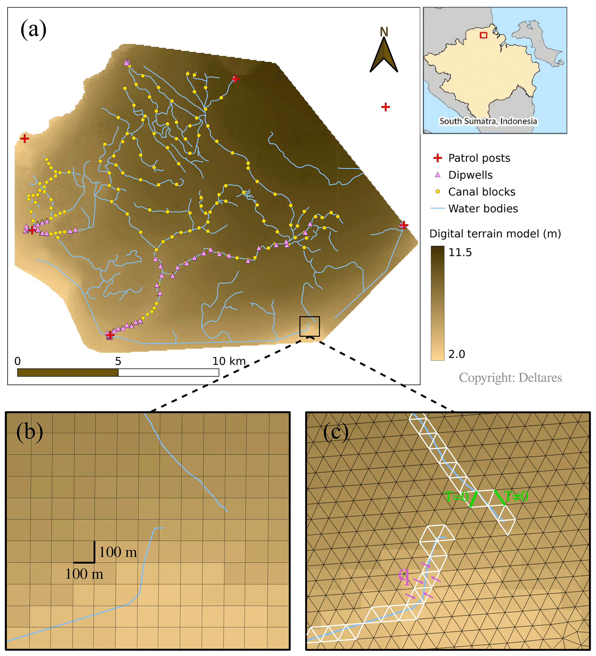
Figure 1Study area and peat hydrological module (PHM) mesh. (a) Digital terrain model (brown gradient), water bodies (blue lines), dipwells (pink triangles), canal blocks (yellow dots), and patrol posts (red crosses). Each patrol post consists of a weather station and six daily measured dipwells along a 200 m transect. The rest of the dipwells were measured manually with monthly frequency. Native forest species are the main vegetation cover. The area extends from 2∘5′29′′ S, 104∘3′14′′ E to 1∘57′11′′ S, 104∘14′1′′ E. (b, c) Zoomed-in region near two canals in the southern part of the study area. (b) Original 100 m × 100 m resolution of the digital terrain model, which was later interpolated to 50 m × 50 m. (c) Triangular mesh for the peat hydrological module (PHM). The white segments show the mesh cell faces corresponding to the canals, which were treated differently. This difference is emphasized with the green and pink schematic annotations. Two cell faces are shown in green: one is the cell face between two canal mesh cells and has a null hydraulic transmissivity, T=0, because flow along the canals occurs only in the canal network module (CNM); the other is the cell face between a canal and a peat mesh cell and therefore T≠0 in general. In pink we indicate the lateral inflow per unit length, q, between the peat and canal mesh cells.
2.2 Modeling
We constructed a hydrological model that produces daily WTD maps. The model consists of a canal network module (CNM) and a peat hydrological module (PHM). At each time step, these modules work in an alternate fashion to update the next day’s canal water level (CWL – meters, negative downwards) and WTD across the study area. First, the CNM computes and updates the CWL using the amount of water expected to have flowed in the peatland–canal interface, which was computed by the PHM in the previous time step. Then, the PHM computes and updates the WTD using the newly computed CWL. The PHM allows for bidirectional water flow between the canals and the peatland, but it only updates the state of the WTD not the CWL.
The CWL and the WTD are essentially the same quantity: water height above a common reference datum; therefore, they are described in this text with the same symbol, h. The context is hopefully clear enough for the reader to discriminate between the two. In the following, each module is described in more detail.
2.2.1 Canal network module (CNM)
The CNM solves h in the canal network using a diffusive wave approximation of the open-channel flow equations (Szymkiewicz, 2010). This approximation requires fewer computational resources than a solution of the full equations, making it particularly suitable for catchment-scale peatland areas with complex canal structures. Additionally, it is able to describe the propagation of the water flow both in the upstream and downstream directions, and thus it can represent the upstream influence of dams, a key feature for our intended application. The diffusive wave approximation is derived from the open-channel flow equations by neglecting the two inertial terms in the momentum equation, which results in a gradient of h that depends only on the friction slope (Novák, 2010). Here, we use a formulation of the open-channel flow equations given by the water surface elevation from the reference datum, h [m], and the discharge, Q [m3 s−1], with the friction slope described by Manning's equation (Cunge et al., 1980),
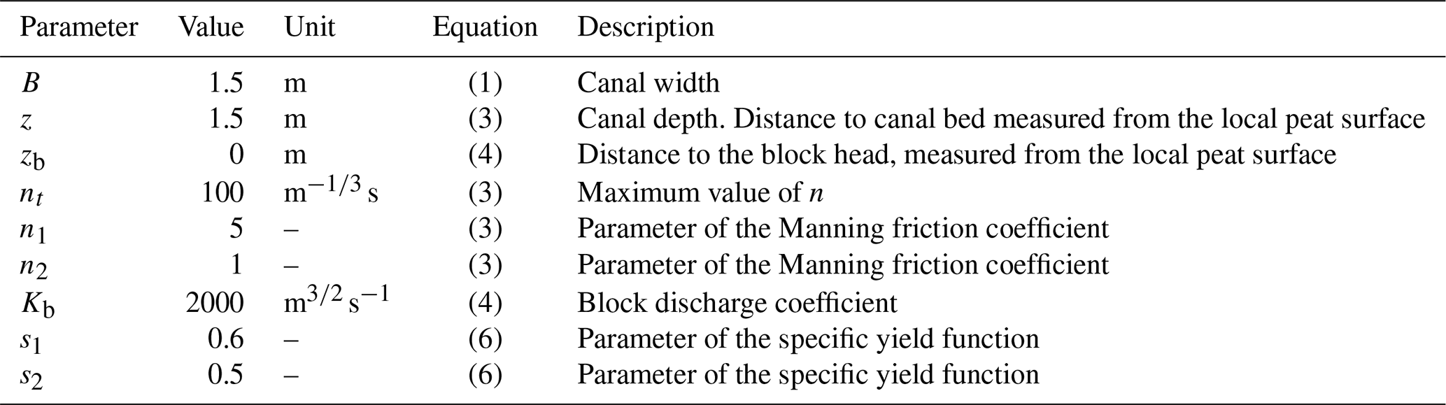
Here, B is the channel width [m], q is the lateral inflow per unit length [], A is the cross-sectional flow area [m2], n is the Manning friction coefficient [], and R is the hydraulic radius [m]. Our model used a simple rectangular channel of height z (i.e., ), where p [m] is the local peat surface (canal bank) elevation above the reference datum. A graphical representation of the variables is shown in Fig. 2, and Table 1 contains the parameter values. The parameters specifying canal geometry – width, depth, and cross-section shape – were determined by local expert observations.
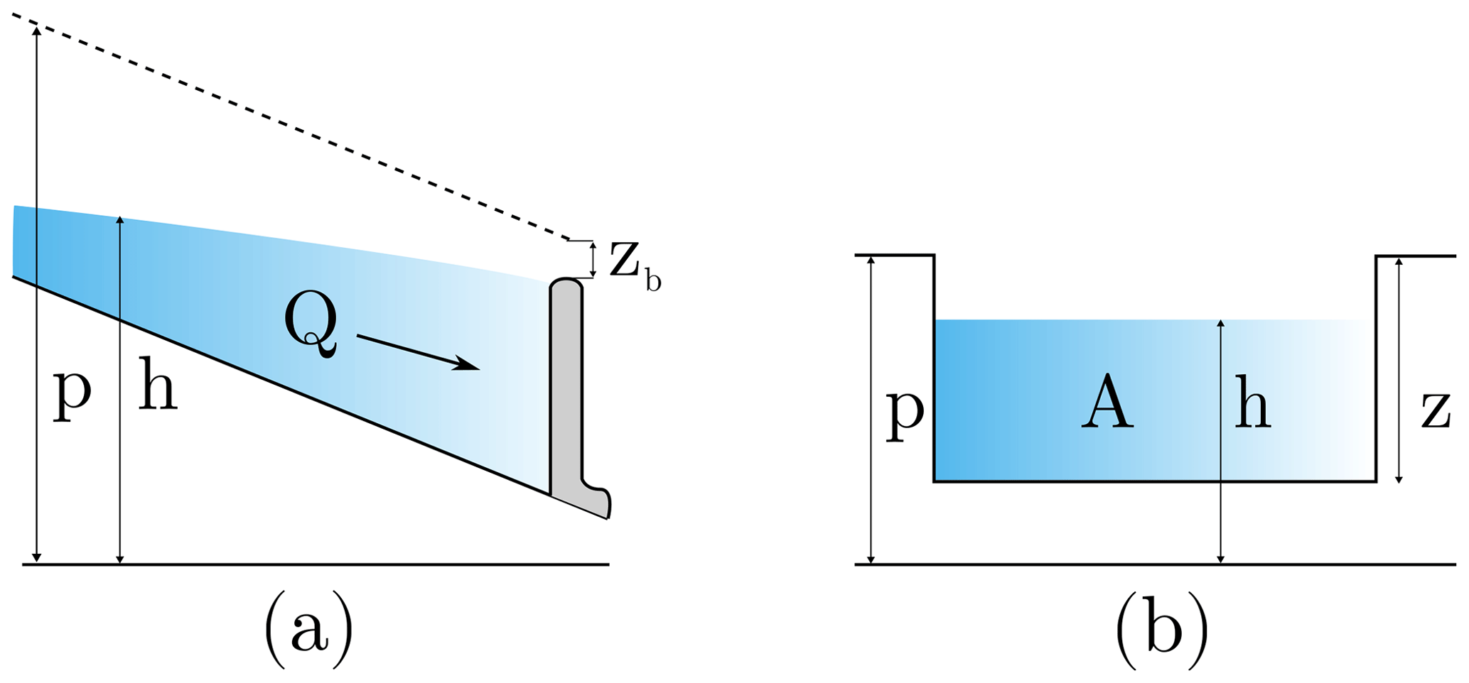
Figure 2Schematic representation of the relevant variables in the open-channel flow equations. (a) Side view and (b) channel cross-section. The gray structure represents a dam.
The mass conservation equation, Eq. (1), may be combined with the momentum equation, Eq. (2), to eliminate one of the dependent variables, h or Q. Usually, h is eliminated to get an advection–diffusion partial differential equation (PDE) for Q (Novák, 2010; Szymkiewicz, 2010). However, here we are interested in the water level in the canal network and thus instead eliminate Q to get a PDE for h. This transformation and the resulting conservative numerical schemes are expressed in detail in Appendix A.
We constructed the Manning friction coefficient n according to these assumptions:
-
The friction increases as the CWL approaches the canal bed. This is due to the resistance to water flow introduced by vegetation growing in the canals and the canal bed surface roughness.
-
When the CWL is below the canal bed, water may still flow through the underlying peat. The friction coefficient in this zone must be several orders of magnitude higher because it is effectively describing water flow in a porous medium.
-
The friction increases with decreasing CWL in a nonlinear fashion.
Therefore, the Manning friction coefficient was described as follows:
Here, nt is a threshold value of n [], and n1 and n2 are parameters. When the CWL drops below the canal bed elevation hb, the Manning friction coefficient is equal to its maximum, nt. For heads above the canal bed, n decreases exponentially with a shape dictated by n1 and n2. In the absence of better information sources, the values for these parameters were chosen so that the value of n when the canal is full of water was n=0.055 , which is in the range described in Szymkiewicz (2010), and the value for flows below the canal bed was n=100 (see Table 1).
The water discharge through a canal block, Qb [m3 s−1], was modeled using the following relationship (Szymkiewicz, 2010):
where Kb [] is a coefficient regulating the rate of water flow through the block, and p−zb [m] is the elevation of the block head above the reference datum (Fig. 2). With this choice, the dam completely blocks water when the CWL is below the block head level. The block discharge coefficient, Kb, was fixed so that the discharge through a block when the CWL was over the block head level was comparable to the discharge through any other node of the computational domain under similar slopes – i.e., Qb≈Q when .
The challenge of solving the open-channel flow equations in a large network of interconnected canals was met with a novel discretization of the equations. As usual, each canal reach was discretized as a one-dimensional grid with a fixed spacing between nodes of Δx=50 m. The novelty introduced by our method concerns the canal junctions. We exploited the basic properties of conservation equations that fully specify the governing equations at every node in the computational domain. This is different from the usual practice, in which external mass and energy conservation equations need to be added manually to the system of equations in order to describe water flow at canal junctions (Cunge et al., 1980). As a result, the computational domain in our method is, by design, analogous to the canal network topology, which simplifies the implementation. Further details on the discretization method are given in Appendix A.
In our numerical implementation of the model, disconnected components of the canal network were solved independently in parallel processes. The accelerated Newton–Raphson method introduced by Liu and Hodges (2014) was used to solve each resulting nonlinear system of equations. No-flow Neumann boundary conditions were set at all boundary nodes.
2.2.2 Peat hydrological module (PHM)
This module uses the output from the CNM to compute the daily WTD in the peat. The approach is similar to the peat hydrological module presented previously in Urzainki et al. (2020) and by many others before that (see, e.g., Cobb et al., 2017; Morris et al., 2012; Putra et al., 2022). We solve the two-dimensional groundwater flow equation, which is suitable for domains that are much wider than they are thick (Connorton, 1985; Bear and Cheng, 2010):
where P−ET [m d−1], the difference between precipitation and evapotranspiration, is the net water input to the system; Sy is the specific yield; and T is the peat hydraulic transmissivity [m2 d−1].
Equation (5) describes water flow through a porous medium. When water ponds above the peat surface, the medium in which water moves is no longer porous, and the physical description of the dynamics of water changes. Our model explicitly separates the two domains (below and above ground) by using a piecewise-defined peat hydraulic transmissivity.
Both the specific yield and the transmissivity are known to vary with WTD. This is especially true of the transmissivity, which may vary by several orders of magnitude in just a few centimeters (Cobb et al., 2017). Following the results of Cobb and Harvey (2019), our model describes the nonlinear variation of Sy and T in the vertical profile with exponential functions. The specific yield was parameterized as
where s1 and s2 are parameters (see Table 2), and ζ is the WTD as measured from the local peat surface [m, negative downwards].
The transmissivity was parameterized as follows:
where d is the local peat thickness [m], and t1 and t2 are parameters (see Table 2).
Below ground, the transmissivity increases exponentially with WTD from a value of when the WTD is at the bottom of the peat column. Above ground, on the contrary, we opted for a constant conductivity, the derivative of transmissivity (), which results in a linear T(ζ). It can be checked that T(ζ) is continuous and differentiable at the domain threshold ζ=0, which helps avoid potential numerical problems.
Equation (5) was solved using an explicit finite-volume solver in an unstructured triangular mesh generated from the study area maps (see Fig. 1c). Convergence and stability of the numerical method were tested by solving the equation with a smaller time step for 5 d ( d was used for the simulations; d was used for the tests). The WTD for the two time steps differed by less than 0.1 % everywhere in the modeled domain (results not shown here). Our code relied on open-source software (Guyer et al., 2009; Geuzaine and Remachle, 2009). Fixed-head Dirichlet boundary conditions with value m were applied at the domain boundaries.
2.2.3 Module interaction
At each time step, the CNM and the PHM are executed in an alternate fashion. The two modules operate in different computational domains, and thus water flow between the canal network and the peat matrix has to be specified externally. On the one hand, the CNM receives information about the peat WTD through the lateral water inflow, q (see Eq. 1). On the other hand, the CWL computed in the same time step is used to populate the PHM mesh cells corresponding to the canal network, thus informing the PHM about the latest CWL status.
In the solution of the PHM, so as not to compute the canal flow twice, water flow between any two adjacent mesh cells that corresponded to the canal network was completely restricted by setting T=0 in the cell faces. In contrast, water flow between canal and peat cells was allowed. The execution of the PHM did not directly modify the CWL; instead, the head difference at canal cells before and after the execution of the PHM was used to compute the lateral water inflow q for each time step. Thus, q acts as a sink or source term which captures how much water is expected to enter or leave each node of the canal network in the next time step. Whenever the CWL rose above ground, the volume of ponding water was distributed instantaneously throughout the corresponding cell area in the PHM step. A schematic representation of the mentioned quantities around canals is shown in Fig. 1c.
An hourly time step was used in each internal iteration ( d), although smaller time steps ( d) were adopted if any of the modules had not converged to a specified accuracy.
2.2.4 Input requirements
The model runs with easily available geospatial data, namely maps of surface elevation and peat depth, as well as a vector file that specifies the topology of the canal network. The digital elevation model and peat depth maps have a resolution of 100 m × 100 m, and they were derived from high-resolution light detection and ranging (lidar) data collected by Deltares following the methods described in Vernimmen et al. (2020). Local depressions in both layers were filled, and the rasters were interpolated to 50 m × 50 m. The peat depth was derived from a geographically weighed regression and spatial interpolation of a peat thickness field inventory. Additionally, daily weather information is required for the solution of Eq. (5). Each cell of the PHM finite-element mesh receives a daily source term input given by the difference between precipitation and evapotranspiration, P−ET. The weather data used in this study differed between model scenarios – see the following section for more details.
2.3 Modeled scenarios
We simulated the WTD over 1 year for eight different scenarios. Each simulation started from the same initial WTD (see Sect. 2.3.5). We ran the model with two different weather data (dry and wet years), two different blocks states (blocked or without any blocks), and two different peat hydraulic transmissivities, T. The eight different scenarios arise from a combination of all of the above factors (23=8).
Apart from those, we also conducted a simple reality check for the model, in which we visually compared the model results with WTD sensor data. The reality check was computed using locally measured weather station data for a single set of values of the peat hydraulic properties. This was only meant as an informal check of the plausibility of our model and was not a part of the main results of this work.
2.3.1 Weather scenarios
The two major components of the water balance in tropical peatlands, precipitation and evapotranspiration, enter the PHM as a net water sink or source term in the PDE – see Eq. (5). Precipitation data were collected from the Sultan Thaha Airport weather station (1∘38′1′′ S, 103∘38′24′′ E), the nearest BMKG (Indonesian Meteorology, Climatology and Geophysics Agency) weather station available. We selected 1 dry year (1997) and 1 wet year (2013) from more than 30 years of data according to total annual rainfall. Net annual water input between the two scenarios differed by 1255 mm: total rainfall in the dry and wet years was 1293.5 and 2584.0 mm, respectively. Around day 150 in the dry scenario, a prolonged dry period began, which lasted almost until the end of the year. The wet year had intense and prolonged rainfalls, even during the dry period. The resulting net water sources for the two scenarios are shown in Fig. 3. The 2 selected years reflect extremes of the large inter-annual and seasonal variability that are common in the tropics.
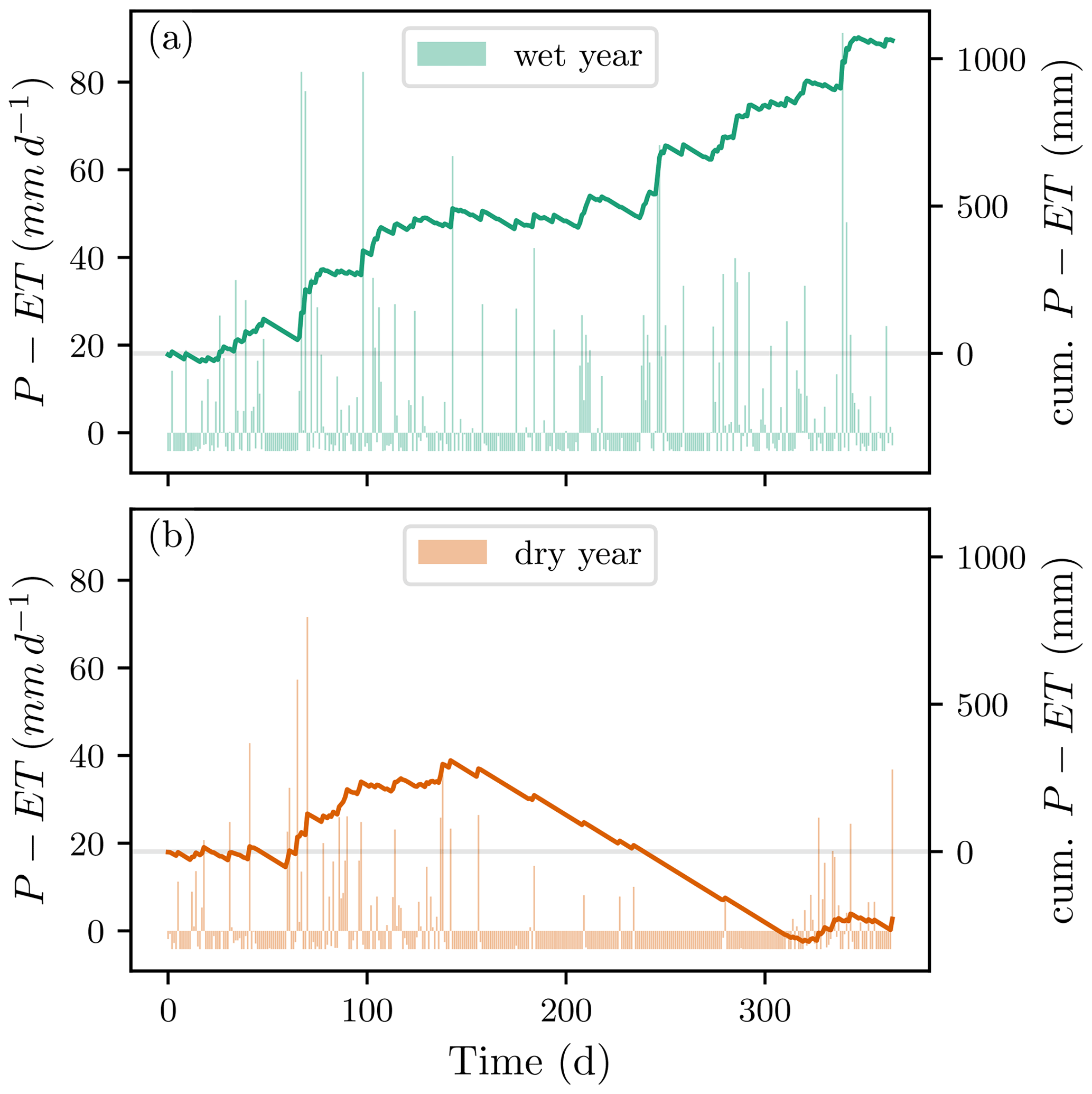
Figure 3Net water source or sink term (precipitation minus evapotranspiration) in the wet (a) and dry (b) modeled scenarios. Vertical bars show daily net water source, and the solid line shows the net cumulative sink or source of water. Note that only the baseline evapotranspiration of ET=4.17 mm d−1 is shown here; the additional contribution due to the pan-evaporation term was dependent on WTD and differed across modeled scenarios.
The evapotranspiration was modeled as a constant daily value plus a pan-evaporation term that only became active when the WTD was close to the peat surface. The variation of evapotranspiration in tropical peatlands is considerably smaller than that of rainfall. This applies to inter-annual variations in total annual evapotranspiration, as well as to daily and seasonal variations within a year (Hirano et al., 2015; Wati et al., 2018). Evapotranspiration enters our model as a quantity relative to precipitation, which justifies our choice of a constant baseline. This value was ET=4.17 mm d−1, the mean of 7 years of measurements across tropical peatlands in different disturbance states (Hirano et al., 2015). Wati et al. (2018) found that pan evaporation (evaporation from ponding water) in Java and Bali could be as high as 7 mm d−1. Based on that, we added a pan-evaporation term to the constant baseline. This pan-evaporation term increased linearly from 0 mm d−1 when the WTD was at −10 cm to 3 mm d−1 when the WTD was at +10 cm. The contribution of the added pan-evaporation term for ponding water tables was cut off at 3 mm d−1.
2.3.2 Block configurations
Two different dam setups were modeled. One setup, which will be referred to as a blocked configuration or simply as blocked, consisted of all the 168 blocks present in the study area (see Fig. 1). The other setup, referred to as not blocked, did not contain any blocks.
2.3.3 Peat hydraulic properties
Our description of the peat hydraulic properties was based on the findings presented in Cobb et al. (2017), Hooijer (2005), and Baird et al. (2017). The values reported for the transmissivity and its derivative, the conductivity, K, vary significantly both between sites and in the vertical soil profile within the same site. In their measurements in several Panamanian peatlands, Baird et al. (2017) found that hydraulic conductivities at a depth of around 0.5 m in the peat profile were in the range K = 7.5–471.9 m d−1. In a Brunei peatland, Cobb et al. (2017) found K=1300 m d−1 at the surface and that K=5.2 m d−1 at 30 cm below the surface. The specific yield, on the other hand, varies less in the cited studies. All values are in the range Sy = 0.29–0.68, with deeper layers of the peat profile having lower values. To capture some of this range and the vertical change in the soil profile, we chose to use a single specific yield curve and two different transmissivity curves, which were modeled using Eqs. (6) and (8). The resulting peat hydraulic properties are shown in Fig. 4, and the sets of parameters used to generate them are listed in Table 2.
Table 2Parameters of the peat hydraulic properties, Eqs. (6) and (8). The peat hydraulic properties resulting from these parameters are shown in Fig. 4. These two sets of parameters were used in different modeled scenarios.
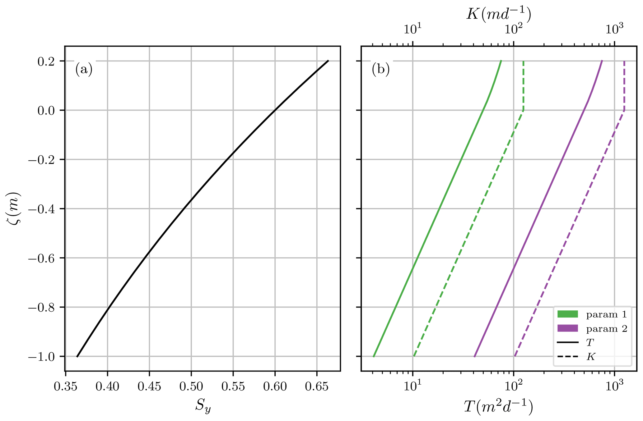
Figure 4The two modeled sets of peat hydraulic properties arising from the parameters in Table 2. (a) Specific yield, Eq. (6), common to all modeled scenarios. (b) Transmissivity, Eq. (8), and its derivative, conductivity, . The different parameter sets are color coded, and this code is used in the rest of the text.
2.3.4 Reality check
We performed a reality check of our model by comparing the simulated WTD with the available measured field data and meteorological data from the patrol posts and dipwell data, both obtained during the year 2020. The variation in peatland topography at smaller scales than the resolution limit of our data (originally 100 m × 100 m) prevented any meaningful one-to-one quantitative comparison between the modeled and the measured WTD (see Fig. 1). This small-scale variation in peat elevation is known to be tens of centimeters (Lampela et al., 2016; Cobb et al., 2017), which is comparable to daily and annual WTD ranges.
The field WTD was measured from the dipwells (see Fig. 1). We modeled the WTD for 1 year for all peat hydraulic properties using the blocked setup.
Precipitation and evapotranspiration were determined using the data collected at the six patrol posts' weather stations (see Fig. 1). The weather data included recordings of daily precipitation, temperature, wind speed, atmospheric pressure, and relative humidity. The daily precipitation was adopted directly from the weather station measurements. The evaporation was modeled using the standard Penman–Montheith equation (Allen et al., 1998), fitting the two free parameters of the model to the annual net radiation and evapotranspiration reported in Hirano et al. (2015). Each cell in the PHM domain received a spatially interpolated daily P−ET value that was based on its distance to the weather stations. We chose to present here the peat hydraulic property set that best fitted the below-ground range and the dynamics of measured WTD.
2.3.5 Initial condition
The initial WTD was the same in all modeled scenarios, including the reality check, and it was derived as follows. Starting from total water saturation, ζ=0 m, everywhere in the study area, we let the model evolve with no precipitation and a high evapotranspiration, ET=7.5 mm d−1. The simulations were run with blocks and with the set of peat hydraulic properties number 2 (see Table 2). The model was run for 50 d, recording the resulting WTD rasters at the end of each day. We then compared the WTD at the dipwell locations for each of the 50 resulting rasters with the dipwell measurements from 22 January 2020, the first sensor measurements of the year. The modeled WTD raster that resulted in the smallest mean squared error was selected as the initial condition for all scenarios. Compared to other possible choices for the initial state of WTD, such as a constant WTD throughout the area, this initial condition captures the natural curvature of the WTD.
2.4 Notation
We will use 〈ζ〉 to indicate the spatially averaged WTD and to indicate the temporal average. Additionally, the quantity
will be used to indicate the WTD difference between two modeled scenarios that only differ by the blocking condition.
2.5 Translation to CO2 emissions
CO2 emissions in the study area were modeled as a linearly increasing function of WTD,
where the negative sign implies that the emissions increase with deeper WTD (note that ζ is negative below ground). Equation (10) was used for below-ground WTD. The CO2 emissions resulting from above-ground WTDs were set to be equal to the emissions at the surface – i.e., . In this work, we used the values from Jauhiainen et al. (2012), a=74.11 and b=29.34 . These values were obtained for an Acacia plantation, which may not give the most accurate estimation of the emissions from a rehabilitating natural peat swamp forest. Therefore the reader is encouraged to treat the CO2 emission results as a rough estimation of their magnitude.
Following the notation introduced in Eq. (9), we will denote the difference in CO2 emissions due to the block influence by .
3.1 Reality check
The comparison between the modeled and the measured WTD shows similarity in the range and the dynamics of WTD, as shown in Fig. 5b. The deepest WTD in both measured and modeled scenarios was about −1.5 m. During most of the year, WTD was between −0.4 and 0.1 m in the majority of the measuring locations. There were two groups of outliers in the sensor data. The sensors with an annual WTD average below −0.7 m corresponded to the easternmost patrol post transect. There were three sensors that recorded an annual WTD average above 0.5 m, but we could not find any pattern to those extreme measurements. The magnitudes of the WTD rise after heavy rainfalls and the WTD drop in the recession periods were similar in the modeled and measured datasets. The water rise and recession slopes were similar as well. As a result, the distribution of annually averaged modeled WTD was similar to the measured one, as can be seen in Fig. 5c.
The model captured the relevant water flow dynamics during the reality check, and thus it is considered to be plausible under the other weather scenarios presented in the study.
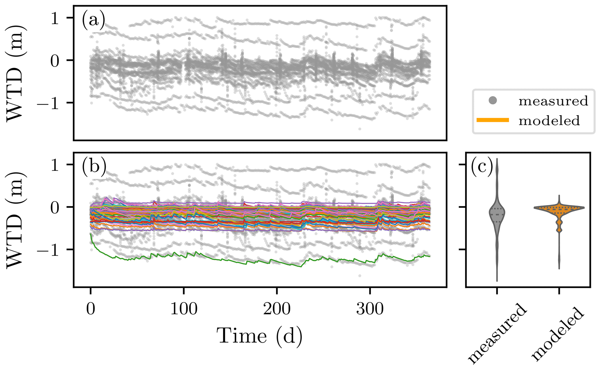
Figure 5Outcome of the reality check. (a) Measured WTD at the 141 dipwells (gray dots). (b) Modeled WTD (colored lines) plotted over the measured WTD of (a) gray dots at the same locations. (c) Kernel density estimation of measured and modeled WTD in (a) and (b). The dotted lines indicate the quartiles of the distribution.
3.2 Block impact on WTD
Blocks led to a net rise of the WTD in all modeled scenarios. This is shown qualitatively in Fig. 6, which aggregates from all modeled scenarios into a single raster. The existence of more areas with a positive (colored in blue in Fig. 6) means that, overall, blocks produced a net WTD rise across all the modeled scenarios. Averaging over all scenarios, the net average WTD rise was 1.51 cm. Despite the overall WTD rise, in some areas, blocks had the effect of lowering WTD compared to the non-blocked scenario (colored in red in Fig. 6). It is also remarkable that the modeled WTD in most of the peatland area far enough from canals (e.g., >1 km) was practically unaffected by the presence or absence of blocks.
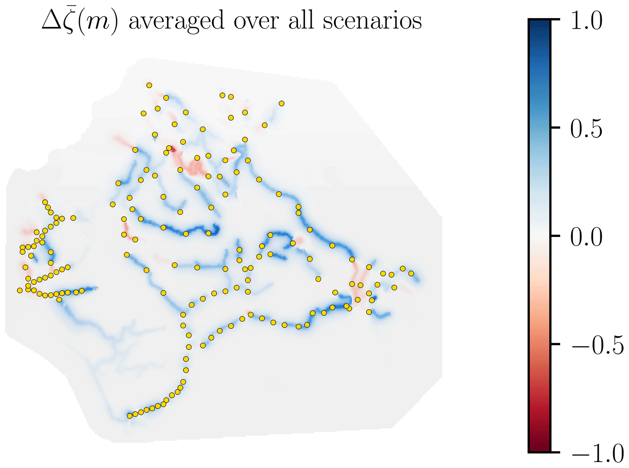
Figure 6Temporal average of the water table depth (WTD) difference between the blocked and non-blocked scenarios, , averaged over all modeled scenarios. Blue and red colors represent the areas in which blocks raised and lowered the WTD, respectively. The gray color present in most of the study area indicates a negligible effect of the blocks on WTD far away from canals – i.e., . The block positions are represented with yellow dots.
The spatially averaged block-induced WTD rise, 〈Δζ〉, differed significantly across different hydraulic property values and weather scenarios, as shown in Fig. 7. However, 〈ζ〉 was always higher with the blocks than without the blocks (positive 〈Δζ〉) for all modeled scenarios. In other words, the overall rewetting impact of the blocks was positive at all times during the simulated period, regardless of weather conditions or peat hydraulic properties.
Figure 7b and c show that rainfall events reduced the difference between the WTD in the blocked and non-blocked scenarios. It may also be seen that, in the dry periods in-between any two large rainfall events, the effect of the blocks was greater. However, dry conditions did not always benefit the blocks' rewetting ability. The extreme drought starting around day 150 in the dry weather scenario shows how canal blocks became less relevant after a certain threshold of external-water-input scarcity. For the first 50 d after the start of the dry period, the gap between blocked and non-blocked WTD increased in the high-transmissivity scenario and stayed relatively constant in the low-transmissivity one (Fig. 7b and d). However, at around day 200, the gap began to close, and by the end of the dry period, blocks were at their minimum effectivity. As a result, the cumulative block-induced WTD rise averaged over peat hydraulic properties was similar in the wet and dry scenarios – 1.44 cm in the dry year and 1.57 cm in the wet year.
Peat hydraulic properties also played an important role in the degree to which blocks were able to raise WTD. Specifically, a larger hydraulic conductivity (or transmissivity) led to greater differences between the blocked and unblocked scenarios in both weather conditions (Fig. 7c and d). Averaged over the two weather conditions, the obtained with the high-transmissivity peat (parameter set 2) was 2.13 times greater than the low-transmissivity one (obtained with parameter set 1) – 2.05 cm versus 0.96 cm.

Figure 7Spatially averaged WTD (a, b) and WTD differences (c, d) between the blocked and non-blocked configurations for all the modeled scenarios. Spatially averaged WTD for wet (a) and dry (b) weather conditions. The solid lines correspond to the blocked scenario, and the dashed lines correspond to the non-blocked. The shaded area between the solid and dashed lines of the same color corresponds to the WTD difference between the two blocking scenarios, 〈Δζ〉, which is explicitly shown in (c) and (d) for clarity. Vertical bars in (c) and (d) show the daily net water input P−ET [m d−1].
There was remarkable variation in the spatial extent of block influence among the different modeling scenarios. As an example, we show two snapshots of Δζ for the high-transmissivity simulation (parameter set 2) in wet and dry years in Fig. 8b and c. These figures qualitatively show that the WTD difference due to the blocks at the end of the wet year was small and concentrated around canals. In contrast, the differences at the end of the dry year were more pronounced and extended further spatially. Note that both the positive and the negative block impacts were larger at the end of the dry year; i.e., Δζ was larger in absolute value. The dependence of on the distance to the nearest block, shown in Fig. 8a), provides a more quantitative description of the spatial extent of block impact. The effect of blocks on WTD for all modeled scenarios was relevant until about 600 m from the nearest dam, and it markedly decreased from there. The mean annual impact of the blocks on WTD more than 1 km away was negligible (not shown in Fig. 8a for clarity). This was true across all weather conditions and peat hydraulic properties, albeit with small variations between modeled scenarios. Higher hydraulic conductivities had the effect of increasing the spatial extent of the blocks' influence.
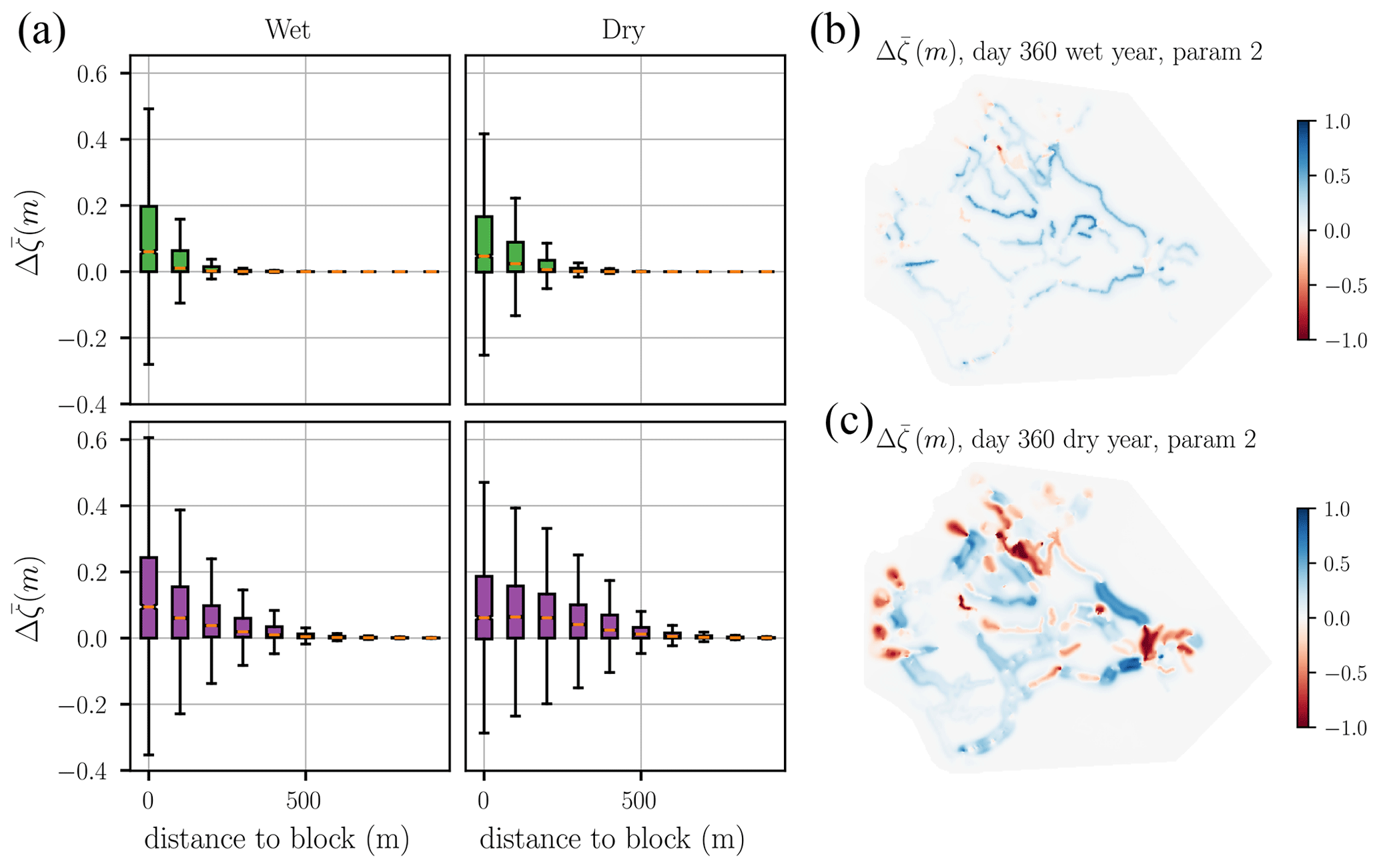
Figure 8Spatial extent of the impact of blocks on WTD. (a) Temporal average of Δζ plotted against the distance to the nearest block, categorized in 100 m classes. The box plot extends from the first to the third quartile, with an orange line at the median. The whiskers extend until 1.5 times the inter-quartile range. Panels (b) and (c) show a snapshot of Δζ at day 360 of the wet (b) and dry (c) years for the high-transmissivity set of peat hydraulic properties (parameter set 2).
3.3 Potential to decrease CO2 emissions
The net block-induced WTD rise in all modeled scenarios led to an overall decrease of CO2 emissions (Fig. 9). In the worst-performing rewetting scenario, with dry conditions and a peatland with the lowest studied hydraulic conductivity (parameter set 1), the non-blocked setup emitted an annual total of 0.62 Mg ha−1 more than the blocked one. In contrast, in the high-transmissivity scenario (parameter set 2), the block-induced WTD rise was translated into a 1.52 CO2 emission reduction for both the dry and wet years. Averaging over peat hydraulic properties, the emission of 1.07 and 1.17 Mg ha−1 CO2 was prevented in the whole year for dry and wet years, respectively.
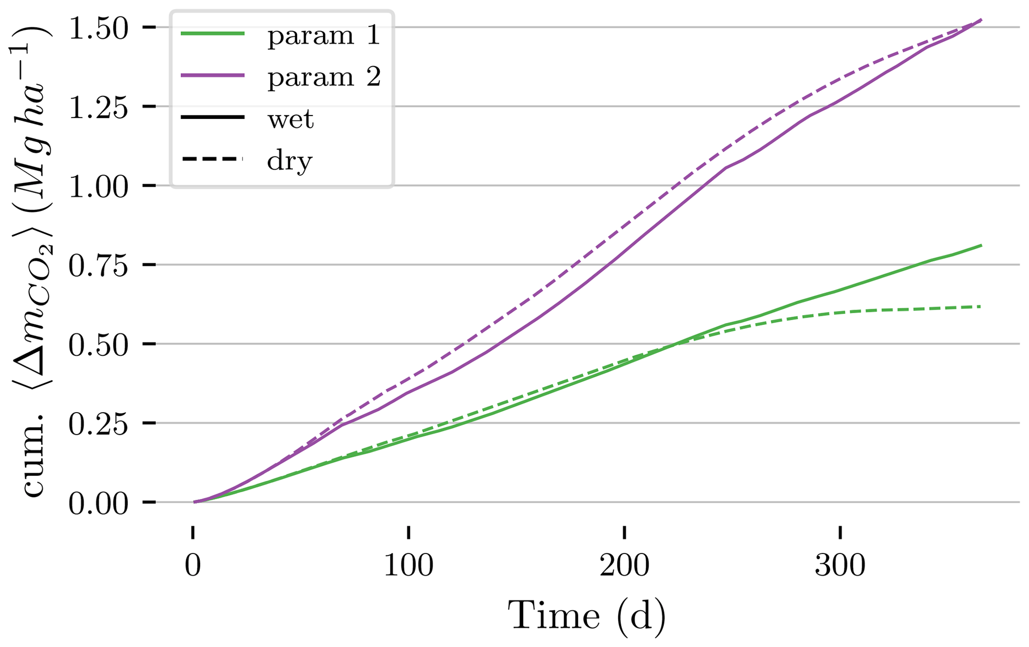
Figure 9Cumulative change in average CO2 emissions due to the blocks, [Mg ha−1], in all modeling scenarios. Positive values indicate lower CO2 emissions in the blocked scenario. Solid and dashed lines correspond to wet and dry weather conditions, while colors stand for different sets of hydraulic peat properties. Sequestered CO2 was computed using a linear relationship with WTD – Eq. (10).
4.1 Comparison to previous studies
A pursuit to estimate the impact of canal blocking in the restoration of tropical peatlands should meet the following four criteria. First, it should capture the complex and interconnected hydrological processes influencing the block performance. Second, the estimation should be done at spatio-temporal scales similar to the specific scale of the restoration project. Third, a method to meaningfully compare blocked and non-blocked scenarios is needed. Finally, in order to make generalizable claims, the sensitivity to weather conditions and peat hydraulic properties should be accounted for.
These criteria are best satisfied with a combination of empirical methods and process-based modeling. If successful, process-based models are able to combine the relevant physical processes governing water flow at sufficiently large scales. Additionally, they offer a direct method to compare different blocking setups and the ability to study the impact of different weather scenarios and peat hydraulic properties. To our knowledge, the present work, which builds upon our previous study (Urzainki et al., 2020), is the first that tries to meet all the aforementioned criteria in tropical peatlands.
A few studies have modeled tropical peatland WTD (Cobb et al., 2017; Cobb and Harvey, 2019; Baird et al., 2012, 2017; Morris et al., 2012; Wösten et al., 2006), but to our knowledge, only three have focused on the effectiveness of canal blocks, namely the studies of Jaenicke et al. (2010), Ishii et al. (2016), and Putra et al. (2022). Both Jaenicke et al. (2010) and Ishii et al. (2016) modeled WTD in large areas and reported that the effect of dams on WTD markedly decayed at 1 km distance from the canals. However, neither of the two works analyzed the effect of different peat hydraulic properties or weather scenarios. The only study that is comparable in scope to ours is that of Putra et al. (2022). Nevertheless, their study area was several orders of magnitude smaller (20 ha), and their CWL was not dynamic but manually fixed to field measurements.
The novelty introduced by our discretization of the open-channel flow equations is also worth underlining. Unlike traditional methods in which junction nodes require a special treatment (Cunge et al., 1980; Novák, 2010), our approach describes the water flow at all nodes of the computational domain with the same equation, Eq. (A8). Our method is automatically applicable to canal networks of arbitrary topology, thus simplifying the model domain-building process.
4.2 Block impact on WTD
Five main outcomes can be drawn from the present study.
First, dams were, on average and across all the modeled scenarios, beneficial for the rewetting of the study area. This has been observed in many studies in tropical and temperate peatlands (Putra et al., 2021; Sutikno et al., 2019, 2020; Holden et al., 2017; Planas-Clarke et al., 2020; Schimelpfenig et al., 2014; Kasih et al., 2016). Canal blocks are mechanisms that increase water residence time in the peatland system, and as a result, they can only raise the average WTD. In turn, assuming a strictly positive impact of WTD rise in terms of CO2 emission reduction, this implies that dams must reduce CO2 emissions overall. However, in line with previous studies (Putra et al., 2021, 2022), dams were not enough to maintain WTD above the −40 cm limit set by the Indonesian Peatland Regulation Agency everywhere in the peatland during the extremely dry year (see Republic of Indonesia Government Regulation No. 57 Year 2016 about Peatland Ecosystem Protection and Management, 2016).
Second, despite raising the WTD on average, blocks did not do so everywhere in the study area. In some areas downstream from the dams, the WTD was systematically lower in the blocked scenario than in its non-blocked counterpart. To our knowledge, such an effect has not been reported in the literature. Our interpretation of this result is straightforward: the function of dams is to block water, and thus they may reduce water supply to areas with a specific combination of local canal network topology and peat topography.
Third, we found that the impact of dams on WTD was confined to areas close to the blocks. The WTD difference between the blocked and non-blocked scenarios was, on average, 3 cm at 400 m from the canals, and it was 1 mm at a 1 km distance (see Fig. 8). Several studies support this claim (Sutikno et al., 2019, 2020; Evans et al., 2019; Putra et al., 2021, 2022; Ishii et al., 2016; Jaenicke et al., 2010). Sutikno et al. (2019), using dipwell measurements, claimed that the radius of action of dams in tropical peatlands is around 170 m, and Ishii et al. (2016) found the modeled WTD rise due to blocks to be about 10 cm at a distance of 400 m. On the one hand, this result confirms that canal blocks are effective in raising the WTD close to the canals, which is where they are most needed. On the other hand, it suggests that naively extrapolating WTD measurements performed in the vicinity of the canals may lead to an incorrect assessment of the ability of blocks to raise WTD throughout the study area.
Fourth, peat hydraulic conductivity had a great impact in terms of the extent to which dams were able to raise the WTD. This effect was also observed in Putra et al. (2022), where blocks had more impact in the higher-conductivity site. Peat hydraulic properties govern the dynamics of groundwater flow, and in particular, the conductivity (or, in our model, the transmissivity) determines the rate of horizontal water flow (Hillel, 1998; Bear and Cheng, 2010). It follows that higher conductivities result in greater responses of WTD to modifications in the CWL. This implies that peatlands with higher hydraulic conductivities have greater potential for greenhouse gas emission mitigation using canal-blocking restoration.
Fifth, the effect of the weather on the block rewetting ability was non-trivial, with an overall slightly greater impact in the wet year than in the dry year. On the one hand, heavy rainfall events led to smaller differences between the blocked and non-blocked scenarios. And it was in the drier days in between these large rainfall events that the blocks were most effective. Our interpretation of these observations is that, with enough water supply from precipitation, WTD rises regardless of whether dams exist or not, making dams less useful. On the other hand, in extremely prolonged dry periods such as the second half of the dry year, the overall rewetting potential of the dams decreased. This behavior agreed with the findings of Putra et al. in their small-scale empirical and modeling studies (Putra et al., 2021, 2022). Putra et al. reported a decrease in the effectiveness of blocks during dry periods because canals became completely dry, and therefore, blocks were not able to retain any water. However, our simple model of discharge through blocks, Eq. (4), completely restricts water flow through blocks even when the water is below the canal bottom, i.e., when the canal is dry. Even if the canals had dried out, our model would not have been able to reproduce the effect described by Putra et al. Thus, another mechanism must explain the observed behavior. Our suspicion is that a combination of the mentioned block impermeability and the low resolution of the data around canals might be responsible. Two consecutive watertight dams in the same canal reach create a segment that is completely disconnected from other parts of the network. The only water source of that canal segment is either precipitation or incoming water from the peatland. Given its low resolution, the digital terrain model (DTM) was not able to describe the usual depressions of the peat surface around canals, which likely reduced the water inflow from the peatland. As a result, some canal segments, embedded in peatland areas with a certain topography, may have received very little water during long dry periods. In our simulations, the negative Δζ arising from those areas decreased faster than the positive Δζ increased in the rest of the areas, hence the overall decrease in the block rewetting ability after a prolonged dry period. In reality, blocks are permeable, although less conductive than an open channel, and canals are excavated in the peat, which attracts more water from the peatland. Therefore, our results in this regard are likely an exaggeration of a subtler effect that takes place in nature. The conclusion that can be drawn from the combination of Putra's and our studies regarding the influence of weather is the following. The WTD difference between the blocked and non-blocked scenarios is generally greater in the absence of rainfall. Blocks are likely to delay the point at which canals become dry; yet, once that point is reached, blocks cease to have any impact on WTD. When water input into the system is scarce, some areas of a blocked peatland might receive considerably less water than an unmanaged one.
4.3 Model limitations
Applications of process-based models have two main sources of uncertainty: the simplifying assumptions made in the construction of the model and the uncertainty in the input data.
The PHM and the CNM use well-established partial differential equations to approximate water flow in peat and in canals. Despite being two dimensional, the groundwater flow equation of the PHM has been shown to accurately represent water movement in such domains where the width exceeds the thickness (Connorton, 1985). The two-dimensional approximation has been used extensively in modeling of hydrology in tropical peatlands (Baird et al., 2012; Cobb et al., 2017). When building the CNM, we tested the diffusive wave approximation against the full open-channel flow equations (Preissmann method; Cunge et al., 1980; Haahti et al., 2014) and concluded that the diffusive wave approximation was accurate enough for this application (testing not shown in this study). This was, in part, because the daily time step was long enough to remove the effect of the inertial terms present in the full open-channel flow equations. As was pointed out previously, the blocks were modeled as watertight barriers that extend from the surface to the impermeable bottom, while in reality they are relatively porous (Osaki and Tsuji, 2016; Ritzema et al., 2014). The coupling between the PHM and CNM approximates water balance, but it does not strictly conserve mass. However, this is an unavoidable drawback of any hydrological model that solves groundwater and surface water flow in different modules (Barthel and Banzhaf, 2016). The error introduced in the coupling was not estimated in this work and is left for future studies, which could use techniques analogous to the ones presented in Gasda et al. (2011).
The lack of information about the water flow at the area boundaries hindered the choice of appropriate boundary conditions in both the PHM and the CNM. In particular, there were no data on the water discharge at the catchment outlet, and we set the boundary conditions in the CWL at that point to no-flow Neumann. This choice, although striking at first, is overrun in the PHM step by the fixed −0.2 m Dirichlet boundary conditions. The Dirichlet boundary conditions are themselves a source of inaccuracy in the simulated WTD, as would be the case with any choice of boundary conditions. It seems plausible that the distance to which the signal of the Dirichlet boundary conditions can propagate over the timescale of the simulation may be similar to the distance to which a change in the CWL affects WTD. Given our results in the present study, we can estimate that inaccuracies introduced by the Dirichlet boundary conditions would only affect the WTD up to a 1 km buffer zone around the boundaries of the study area. We nevertheless argue that these inaccuracies do not undermine the results presented in this work because they are based on direct comparisons between different scenarios. Indeed, the WTD difference maps displayed in Figs. 6 and 8b and c confirm that the difference between scenarios is negligible at the study area boundaries. It is reasonable to think then that most of the error introduced by the boundary conditions does not have a large effect on our results.
Despite being crucial for the understanding of water dynamics, there exist few published measurements of the physical parameters which govern water flow in tropical peat and in canals. Whereas the variability of the peat hydraulic properties was taken into account through the different modeling scenarios, the physical parameters governing open-channel flow were fixed in all the scenarios. In reality, all these – the width, depth, and cross-section shape of the canals; the block discharge coefficient; and the Manning friction coefficient – vary spatially and/or temporally (Ritzema et al., 2014; Osaki and Tsuji, 2016). Since the value of these coefficients has a direct influence on water dynamics, more experimental work is needed to correctly quantify the open-channel flow coefficients for tropical peatlands. One positive point of this study, however, is that the large study area naturally included some variability in terms of the location of canals and blocks. The western part of the catchment, for instance, had more blocks per unit area than the southeastern part. This helped to capture some of the spectrum of canal and block densities typically present in tropical restoration projects without having to explicitly include it in the study design. Indeed, this heterogeneity is represented in the variance of the block impact in Fig. 8.
Not only the CNM parameters but also the physical parameters of the PHM are expected to have some spatial variability too. Peat hydraulic properties are known to vary with vegetation and land use (Baird et al., 2017; Kurnianto et al., 2019), and even precipitation and evapotranspiration may change over the study area (Vijith and Dodge-Wan, 2020). Our model could accommodate all this spatial variability, but in the absence of data, we were forced to assume constant values throughout the study area.
The model validation against the dipwell-measured WTD was limited by the coarse resolution of the PHM computational domain. The original resolution of our digital elevation model was 100 m × 100 m, a scale at which tropical peat surface typically presents variations on the order of tens of centimeters (Lampela et al., 2016). In the absence of further information about the precise elevation of the dipwells, we assumed an uncertainty of comparable magnitude in the dipwell WTD measurements. And since WTD variation at any location was also on the order of tens of centimeters (see Fig. 5), this uncertainty prevented any direct quantitative comparison between the modeled and measured WTD. As a result, we resorted to doing a qualitative estimation of the model plausibility (see “Reality check”, Sects. 2.3.4 and 3.1). Two main features of the reality check of Fig. 5 support the validity of the model. First, the model was unbiased, and the range of modeled and measured WTD was comparable. Second, the modeled WTD presented similar ranges and slopes in the daily dynamics driven by precipitation and evapotranspiration. The origin of the dipwell measurements showing WTD up to 1 m above the surface in Fig. 5 is unknown to us. They could be due to a wrong datum or due to local depressions that are unnoticeable in the DTM, which canalize the water to certain spots.
The coarse resolution also prevented precise modeling of the canal–peatland interface (see Fig. 1b and c). This may have led to an underestimation of the water gradient between the canals and the peatland and therefore also to low CWL in very dry conditions (see fifth point in the previous section).
Despite the presented limitations, we claim that the modeling setup presented here has a greater potential to study the rewetting ability of blocks than purely experimental studies have. On the one hand, the effect of some of the aforementioned uncertainties might be partially compensated for by the fact that we have only presented relative comparisons between blocked and non-blocked scenarios. On the other hand, our model gives theoretically coherent estimates of the dam impact throughout the area, which is not possible to do with experimental studies alone.
4.4 Further study
The present work was limited to the analysis of a single study area, with one block location configuration, for a relatively short period of time. Future studies might consider how varying the number of dams and their positions affects WTD, since, as we know, the dam position is critical (Urzainki et al., 2020). Furthermore, the impact of blocks on WTD would probably change on timescales of decades, which is closer to the typical lifespan of canal blocks (Ritzema et al., 2014; Dohong et al., 2018). When analyzing long-term scenarios, the effect of climate change on precipitation and evapotranspiration (Gallego-Sala et al., 2018; Wang et al., 2018; Cai et al., 2014; Pörtner et al., 2022), as well as on peat subsidence (Evans et al., 2019; Hoyt et al., 2020; Evans et al., 2022), will need to be addressed.
In order to have a more precise estimate of greenhouse gas emissions, future studies should take into account emissions of other compounds, such as methane and nitrous oxides. In fact, having shallower WTD as the only optimization goal may not be desirable due to increased methane emissions – although we are not aware of any studies where methane emissions have been shown to surpass CO2 emissions (Teh et al., 2017; Wong et al., 2018; Planas-Clarke et al., 2020; Deshmukh et al., 2020, 2021; Kiuru et al., 2022; Zou et al., 2022; Lestari et al., 2022).
It might be interesting to connect process-based models such as the one presented in this work not only with more extensive empirical studies but also with state-of-the-art remote sensing techniques for WTD measurement, such as in Hikouei et al. (2023).
We modeled the effect that canal block restoration practices had on the WTD of a 22 000 ha drained tropical peatland. Our results show that the blocks raised WTD on average, but their effect was limited. Block impact on WTD at a distance of 1 km was negligible during 1 year of simulations, and blocks lowered the WTD in some areas. The effect of dams was largest during dry periods and in peat soils with higher hydraulic conductivities. We believe that the present modeling setup, which has been designed with stakeholders' practical management questions in mind, could be adopted by local agencies aiming at a more effective and evidence-based approach to canal-block-based peatland restoration.
The open-channel flow Eqs. (1) and (2) must be solved in a network of connected channel segments. This connectivity gives rise to a type of computational node that does not exist when the channel segments are modeled individually: the junction node, a node shared by more than one individual channel. The traditional discretization of the equations involves writing the numerical approximations for each individual channel reach first and then manually adding some mass and energy conservation conditions at the junction nodes (Cunge et al., 1980; Szymkiewicz, 2010). However, in large and complex channel networks, the traditional approach is tedious and error prone because all conservation equations at junctions need to be introduced manually. In this work, we used a slightly different conceptual approach to derive the numerical discretization of the open-channel flow equations that allows us to set up the linear system directly from the channel network topology.
The first equation of the open-channel flow equations, Eq. (1), is the mass conservation equation. In general, differential equations that describe conservation laws in one dimension take the following form:
where u is the conserved quantity, and f(u) is the rate of the flow or flux of the conserved quantity.
Let us discretize space and time with regular meshes of width Δx and time step Δt and define the discrete mesh points xi=iΔx and tn=nΔt with i and n ∈ℕ. Conservative numerical methods are those that can be written as
for implicit schemes and analogously for explicit schemes (LeVeque, 1992). In the simplest case (p=0 and q=1), this becomes
The function , called the numerical flux function, plays the role of the average flux of the conserved quantity u, f(u), between xi and xi+1 during the time interval .
The system of equations arising from the discretization of Eq. (A3) may be interpreted as balance equations at every node. Indeed, the form of Eq. (A3) ensures that what appears with a plus sign in the equation for ui must appear with a minus sign in the equation for ui+1. Therefore, the total quantity of the conserved variable u in any region changes only due to flux through the boundaries.
We may impose this same condition for a general junction node with more than two neighbors. Let us denote the index of the junction node as J, and let in and out be the set of nodes whose flux is incoming and outgoing from J, respectively. Then, the discretized equation for the conservative method at a general junction node is
Note that Eq. (A4) reduces to Eq. (A3) for interior nodes. Requiring conservativeness of the numerical scheme at junctions fully specifies the form of the discretized equations. Equation (A4) provides the blueprint for a conservative numerical scheme that is applicable to all nodes in the computational domain.
Our numerical method to solve the mass conservation equation, Eq. (1), is obtained by setting the numerical flux function from node i to node k to be equal to , the water discharge between those two nodes. The discretization equation for any node in the channel network domain is then
Note that, in our model, the channel width B is the same for every node – i.e., Bi=B.
The second equation of the diffusive wave approximation, Eq. (2), now becomes useful. It relates the magnitude of the discharge Q to the square root of the gradient of the water elevation,
where .
A straightforward discretization of the spatial derivative results in
where is the magnitude of the water discharge between nodes i and k, and .
Finally, we insert Eq. (A7) in Eq. (A5) to get our numerical scheme for the diffusive wave approximation of the open-channel flow equations,
The sign function accounts for the direction of the water flow (note the negative sign of Eq. 2), and the sum in k goes over all neighboring nodes of the node i. As we noted previously, this equation is valid for all nodes in the computational domain, including junction nodes.
With a judicious use of the information about the channel network topology (e.g., by using the adjacency matrix of the graph of canal nodes), this discretization enables a simple implementation of the diffusive wave approximations, since junction nodes do not need to be accounted for separately.
The source code and all the data (except the DTM, which is property of Deltares) are available at https://doi.org/10.5281/zenodo.7908069 (Urzainki, 2023a). Forest Carbon PTE LTD (https://forestcarbon.com/, last access: 1 November 2022) provided the data.
Animations of for all modeled scenarios are available at https://doi.org/10.5281/zenodo.7791585 (Urzainki, 2023b).
IU and AL formulated the research goals and methods. IU developed the model code, performed the simulations, and prepared the article. MP, HH, and AL reviewed and edited the article. SP, JC, OW, PM, and RY produced and validated the datasets.
The contact author has declared that none of the authors has any competing interests.
Publisher’s note: Copernicus Publications remains neutral with regard to jurisdictional claims in published maps and institutional affiliations.
The authors wish to acknowledge CSC – IT Center for Science, Finland, for the computational resources.
This paper was edited by Alexandra Konings and reviewed by Alex Cobb and Santosa Sandy Putra.
Allen, R., Pereira, L., Raes, D., and Smith, M.: Crop Evapotranspiration, Guidelines for Computing Crop Water Requirements, FAO, p. 300, 1998. a
Baird, A. J., Morris, P. J., and Belyea, L. R.: The DigiBog Peatland Development Model 1: Rationale, Conceptual Model, and Hydrological Basis, Ecohydrology, 5, 242–255, https://doi.org/10.1002/eco.230, 2012. a, b
Baird, A. J., Low, R., Young, D., Swindles, G. T., Lopez, O. R., and Page, S.: High Permeability Explains the Vulnerability of the Carbon Store in Drained Tropical Peatlands, Geophys. Res. Lett., 44, 1333–1339, https://doi.org/10.1002/2016GL072245, 2017. a, b, c, d, e
Barthel, R. and Banzhaf, S.: Groundwater and Surface Water Interaction at the Regional-scale – A Review with Focus on Regional Integrated Models, Water Resour. Manag., 30, 1–32, https://doi.org/10.1007/s11269-015-1163-z, 2016. a
Bear, J. and Cheng, A. H.-D.: Modeling Groundwater Flow and Contaminant Transport, edited by: Bear, J., Springer Netherlands, Dordrecht, https://doi.org/10.1007/978-1-4020-6682-5, 2010. a, b
Cai, W., Borlace, S., Lengaigne, M., van Rensch, P., Collins, M., Vecchi, G., Timmermann, A., Santoso, A., McPhaden, M. J., Wu, L., England, M. H., Wang, G., Guilyardi, E., and Jin, F.-F.: Increasing Frequency of Extreme El Niño Events Due to Greenhouse Warming, Nat. Clim. Change, 4, 111–116, https://doi.org/10.1038/nclimate2100, 2014. a
Carlson, K. M., Goodman, L. K., and May-Tobin, C. C.: Modeling Relationships between Water Table Depth and Peat Soil Carbon Loss in Southeast Asian Plantations, Environ. Res. Lett., 10, 074006, https://doi.org/10.1088/1748-9326/10/7/074006, 2015. a
Cobb, A. R. and Harvey, C. F.: Scalar Simulation and Parameterization of Water Table Dynamics in Tropical Peatlands, Water Resour. Res., 55, 9351–9377, https://doi.org/10.1029/2019WR025411, 2019. a, b
Cobb, A. R., Hoyt, A. M., Gandois, L., Eri, J., Dommain, R., Abu Salim, K., Kai, F. M., Haji Su'ut, N. S., and Harvey, C. F.: How Temporal Patterns in Rainfall Determine the Geomorphology and Carbon Fluxes of Tropical Peatlands, P. Natl. Acad. Sci. USA, 114, 201701090, https://doi.org/10.1073/pnas.1701090114, 2017. a, b, c, d, e, f, g, h
Connorton, B.: Does the Regional Groundwater-Flow Equation Model Vertical Flow?, J. Hydrol., 79, 279–299, https://doi.org/10.1016/0022-1694(85)90059-9, 1985. a, b
Cunge, J. A., Holly, F. M., and Verwey, A.: Practical Aspects of Computational River Hydraulics, no. 3 in Monographs and Surveys in Water Resources Engineering, Pitman Advanced Pub. Program, Boston, 1980. a, b, c, d, e
Deshmukh, C. S., Julius, D., Evans, C. D., Nardi, Susanto, A. P., Page, S. E., Gauci, V., Laurén, A., Sabiham, S., Agus, F., Asyhari, A., Kurnianto, S., Suardiwerianto, Y., and Desai, A. R.: Impact of Forest Plantation on Methane Emissions from Tropical Peatland, Glob. Change Biol., 26, 2477–2495, https://doi.org/10.1111/gcb.15019, 2020. a
Deshmukh, C. S., Julius, D., Desai, A. R., Asyhari, A., Page, S. E., Nardi, N., Susanto, A. P., Nurholis, N., Hendrizal, M., Kurnianto, S., Suardiwerianto, Y., Salam, Y. W., Agus, F., Astiani, D., Sabiham, S., Gauci, V., and Evans, C. D.: Conservation Slows down Emission Increase from a Tropical Peatland in Indonesia, Nat. Geosci., 14, 484–490, https://doi.org/10.1038/s41561-021-00785-2, 2021. a
Dohong, A., Aziz, A. A., and Dargusch, P.: A Review of the Drivers of Tropical Peatland Degradation in South-East Asia, Land Use Policy, 69, 349–360, https://doi.org/10.1016/j.landusepol.2017.09.035, 2017. a, b
Dohong, A., Abdul Aziz, A., and Dargusch, P.: A Review of Techniques for Effective Tropical Peatland Restoration, Wetlands, 38, 275–292, https://doi.org/10.1007/s13157-018-1017-6, 2018. a, b, c
Evans, C. D., Williamson, J. M., Kacaribu, F., Irawan, D., Suardiwerianto, Y., Hidayat, M. F., Laurén, A., and Page, S. E.: Rates and Spatial Variability of Peat Subsidence in Acacia Plantation and Forest Landscapes in Sumatra, Indonesia, Geoderma, 338, 410–421, https://doi.org/10.1016/j.geoderma.2018.12.028, 2019. a, b, c
Evans, C. D., Irawan, D., Suardiwerianto, Y., Kurnianto, S., Deshmukh, C., Asyhari, A., Page, S., Astiani, D., Agus, F., Sabiham, S., Laurén, A., and Williamson, J.: Long-Term Trajectory and Temporal Dynamics of Tropical Peat Subsidence in Relation to Plantation Management and Climate, Geoderma, 428, 116100, https://doi.org/10.1016/j.geoderma.2022.116100, 2022. a, b
Gallego-Sala, A. V., Charman, D. J., Brewer, S., Page, S. E., Prentice, I. C., Friedlingstein, P., Moreton, S., Amesbury, M. J., Beilman, D. W., Björck, S., Blyakharchuk, T., Bochicchio, C., Booth, R. K., Bunbury, J., Camill, P., Carless, D., Chimner, R. A., Clifford, M., Cressey, E., Courtney-Mustaphi, C., De Vleeschouwer, F., de Jong, R., Fialkiewicz-Koziel, B., Finkelstein, S. A., Garneau, M., Githumbi, E., Hribjlan, J., Holmquist, J., Hughes, P. D. M., Jones, C., Jones, M. C., Karofeld, E., Klein, E. S., Kokfelt, U., Korhola, A., Lacourse, T., Le Roux, G., Lamentowicz, M., Large, D., Lavoie, M., Loisel, J., Mackay, H., MacDonald, G. M., Makila, M., Magnan, G., Marchant, R., Marcisz, K., Martínez Cortizas, A., Massa, C., Mathijssen, P., Mauquoy, D., Mighall, T., Mitchell, F. J. G., Moss, P., Nichols, J., Oksanen, P. O., Orme, L., Packalen, M. S., Robinson, S., Roland, T. P., Sanderson, N. K., Sannel, A. B. K., Silva-Sánchez, N., Steinberg, N., Swindles, G. T., Turner, T. E., Uglow, J., Väliranta, M., van Bellen, S., van der Linden, M., van Geel, B., Wang, G., Yu, Z., Zaragoza-Castells, J., and Zhao, Y.: Latitudinal Limits to the Predicted Increase of the Peatland Carbon Sink with Warming, Nat. Clim. Change, 8, 907–913, https://doi.org/10.1038/s41558-018-0271-1, 2018. a
Gasda, S. E., Farthing, M. W., Kees, C. E., and Miller, C. T.: Adaptive Split-Operator Methods for Modeling Transport Phenomena in Porous Medium Systems, Adv. Water Resour., 34, 1268–1282, https://doi.org/10.1016/j.advwatres.2011.06.004, 2011. a
Geuzaine, C. and Remachle, J.-F.: Gmsh: A Three-Dimensional Finite Element Mesh Generator with Built-in Pre- and Post-Processing Facilities, Int. J. Numer. Meth. Eng., 79, 1309–1331, 2009. a
Guyer, J. E., Wheeler, D., and Warren, J. A.: FiPy: Partial Differential Equations with Python, Comput. Sci. Eng., 11, 6–15, https://doi.org/10.1109/MCSE.2009.52, 2009. a
Haahti, K., Younis, B. A., Stenberg, L., and Koivusalo, H.: Unsteady Flow Simulation and Erosion Assessment in a Ditch Network of a Drained Peatland Forest Catchment in Eastern Finland, Water Resour. Manag., 28, 5175–5197, https://doi.org/10.1007/s11269-014-0805-x, 2014. a
Hikouei, I. S., Eshleman, K. N., Saharjo, B. H., Graham, L. L. B., Applegate, G., and Cochrane, M. A.: Using Machine Learning Algorithms to Predict Groundwater Levels in Indonesian Tropical Peatlands, Sci. Total Environ., 857, 159701, https://doi.org/10.1016/j.scitotenv.2022.159701, 2023. a
Hillel, D.: Environmental Soil Physics, Academic Press, San Diego, CA, ISBN 978-0-12-348525-0, 1998. a
Hirano, T., Kusin, K., Limin, S., and Osaki, M.: Evapotranspiration of Tropical Peat Swamp Forests, Glob. Change Biol., 21, 1914–1927, https://doi.org/10.1111/gcb.12653, 2015. a, b, c
Holden, J., Green, S. M., Baird, A. J., Grayson, R. P., Dooling, G. P., Chapman, P. J., Evans, C. D., Peacock, M., and Swindles, G.: The Impact of Ditch Blocking on the Hydrological Functioning of Blanket Peatlands: Blanket Peat Ditch Blocking Impacts, Hydrol. Process., 31, 525–539, https://doi.org/10.1002/hyp.11031, 2017. a
Hooijer, A.: Hydrology of Tropical Wetland Forests: Recent Research Results from Sarawak Peatswamps, in: Forests, Water and People in the Humid Tropics, edited by: Bonell, M. and Bruijnzeel, L. A., 447–461, Cambridge University Press, 1st Edn., https://doi.org/10.1017/CBO9780511535666.023, 2005. a
Hooijer, A., Page, S., Jauhiainen, J., Lee, W. A., Lu, X. X., Idris, A., and Anshari, G.: Subsidence and carbon loss in drained tropical peatlands, Biogeosciences, 9, 1053–1071, https://doi.org/10.5194/bg-9-1053-2012, 2012. a
Hoyt, A. M., Chaussard, E., Seppalainen, S. S., and Harvey, C. F.: Widespread Subsidence and Carbon Emissions across Southeast Asian Peatlands, Nat. Geosci., 13, 435–440, https://doi.org/10.1038/s41561-020-0575-4, 2020. a, b
Ishii, Y., Koizumi, K., Fukami, H., Yamamoto, K., Takahashi, H., Limin, S. H., Kusin, K., Usup, and Susilo, G. E.: Groundwater in Peatland, in: Tropical Peatland Ecosystem, edited by: Osaki, M. and Tsuji, N., 265–279, Springer Japan, ISBN 978-4-431-55680-0, 2016. a, b, c, d, e, f
Ishikura, K., Hirano, T., Okimoto, Y., Hirata, R., Kiew, F., Melling, L., Aeries, E. B., Lo, K. S., Musin, K. K., Waili, J. W., Wong, G. X., and Ishii, Y.: Soil Carbon Dioxide Emissions Due to Oxidative Peat Decomposition in an Oil Palm Plantation on Tropical Peat, Agr. Ecosyst. Environ., 254, 202–212, https://doi.org/10.1016/j.agee.2017.11.025, 2018. a
Jaenicke, J., Wösten, H., Budiman, A., and Siegert, F.: Planning Hydrological Restoration of Peatlands in Indonesia to Mitigate Carbon Dioxide Emissions, Mitig. Adapt. Strat. Gl., 15, 223–239, https://doi.org/10.1007/s11027-010-9214-5, 2010. a, b, c, d, e, f
Jauhiainen, J., Hooijer, A., and Page, S. E.: Carbon dioxide emissions from an Acacia plantation on peatland in Sumatra, Indonesia, Biogeosciences, 9, 617–630, https://doi.org/10.5194/bg-9-617-2012, 2012. a, b
Kasih, R. C., Simon, O., Ansori, M., Pratama, M. P., and Wirada, F.: Rewetting of Degraded Tropical Peatland by Canal Blocking Technique in Sebangau National Park, Central Kalimantan, Indonesia, in: 15th International Peat Congress, p. 5, Kuching, 2016. a, b
Kiely, L., Spracklen, D. V., Arnold, S. R., Papargyropoulou, E., Conibear, L., Wiedinmyer, C., Knote, C., and Adrianto, H. A.: Assessing Costs of Indonesian Fires and the Benefits of Restoring Peatland, Nat. Commun., 12, 7044, https://doi.org/10.1038/s41467-021-27353-x, 2021. a
Kiuru, P., Palviainen, M., Grönholm, T., Raivonen, M., Kohl, L., Gauci, V., Urzainki, I., and Laurén, A.: Peat macropore networks – new insights into episodic and hotspot methane emission, Biogeosciences, 19, 1959–1977, https://doi.org/10.5194/bg-19-1959-2022, 2022. a
Könönen, M., Jauhiainen, J., Straková, P., Heinonsalo, J., Laiho, R., Kusin, K., Limin, S., and Vasander, H.: Deforested and Drained Tropical Peatland Sites Show Poorer Peat Substrate Quality and Lower Microbial Biomass and Activity than Unmanaged Swamp Forest, Soil Biol. Biochem., 123, 229–241, https://doi.org/10.1016/j.soilbio.2018.04.028, 2018. a
Kurnianto, S., Selker, J., Boone Kauffman, J., Murdiyarso, D., and Peterson, J. T.: The Influence of Land-Cover Changes on the Variability of Saturated Hydraulic Conductivity in Tropical Peatlands, Mitig. Adapt. Strat. Gl., 24, 535–555, https://doi.org/10.1007/s11027-018-9802-3, 2019. a
Lampela, M., Jauhiainen, J., Kämäri, I., Koskinen, M., Tanhuanpää, T., Valkeapää, A., and Vasander, H.: Ground Surface Microtopography and Vegetation Patterns in a Tropical Peat Swamp Forest, Catena, 139, 127–136, https://doi.org/10.1016/j.catena.2015.12.016, 2016. a, b
Laurén, A., Palviainen, M., Page, S., Evans, C., Urzainki, I., and Hökkä, H.: Nutrient Balance as a Tool for Maintaining Yield and Mitigating Environmental Impacts of Acacia Plantation in Drained Tropical Peatland – Description of Plantation Simulator, Forests, 12, 312, https://doi.org/10.3390/f12030312, 2021. a
Lestari, I., Murdiyarso, D., and Taufik, M.: Rewetting Tropical Peatlands Reduced Net Greenhouse Gas Emissions in Riau Province, Indonesia, Forests, 13, 505, https://doi.org/10.3390/f13040505, 2022. a
LeVeque, R. J.: Numerical Methods for Conservation Laws, Lectures in Mathematics ETH Zürich, Birkhäuser Verlag, Basel, Boston, 2nd Edn., ISBN 978-0-898716-29-0, 1992. a
Liu, F. and Hodges, B. R.: Applying Microprocessor Analysis Methods to River Network Modelling, Environ. Modell. Softw., 52, 234–252, https://doi.org/10.1016/j.envsoft.2013.09.013, 2014. a
Miettinen, J., Shi, C., and Liew, S. C.: Land Cover Distribution in the Peatlands of Peninsular Malaysia, Sumatra and Borneo in 2015 with Changes since 1990, Global Ecology and Conservation, 6, 67–78, https://doi.org/10.1016/j.gecco.2016.02.004, 2016. a
Miettinen, J., Shi, C., and Liew, S. C.: Fire Distribution in Peninsular Malaysia, Sumatra and Borneo in 2015 with Special Emphasis on Peatland Fires, Environ. Manage., 60, 747–757, https://doi.org/10.1007/s00267-017-0911-7, 2017. a
Morris, P. J., Baird, A. J., and Belyea, L. R.: The DigiBog Peatland Development Model 2: Ecohydrological Simulations in 2D, Ecohydrology, 5, 256–268, https://doi.org/10.1002/eco.229, 2012. a, b
Novák, P. (Ed.): Hydraulic Modelling: An Introduction, Principles, Methods and Applications, Spon Press, London, New York, ISBN 978-0-419-25010-4, 2010. a, b, c
Novita, N., Lestari, N. S., Lugina, M., Tiryana, T., Basuki, I., and Jupesta, J.: Geographic Setting and Groundwater Table Control Carbon Emission from Indonesian Peatland: A Meta-Analysis, Forests, 12, 832, https://doi.org/10.3390/f12070832, 2021. a
Osaki, M. and Tsuji, N. (Eds.): Tropical Peatland Ecosystems, Springer Japan, Tokyo, https://doi.org/10.1007/978-4-431-55681-7, 2016. a, b
Page, S., Mishra, S., Agus, F., Anshari, G., Dargie, G., Evers, S., Jauhiainen, J., Jaya, A., Jovani-Sancho, A. J., Laurén, A., Sjögersten, S., Suspense, I. A., Wijedasa, L. S., and Evans, C. D.: Anthropogenic Impacts on Lowland Tropical Peatland Biogeochemistry, Nat. Rev. Earth Environ., 3, 426–443, https://doi.org/10.1038/s43017-022-00289-6, 2022. a, b
Page, S. E., Rieley, J. O., and Banks, C. J.: Global and Regional Importance of the Tropical Peatland Carbon Pool, Glob. Change Biol., 17, 798–818, https://doi.org/10.1111/j.1365-2486.2010.02279.x, 2011. a
Planas-Clarke, A. M., Chimner, R. A., Hribljan, J. A., Lilleskov, E. A., and Fuentealba, B.: The Effect of Water Table Levels and Short-Term Ditch Restoration on Mountain Peatland Carbon Cycling in the Cordillera Blanca, Peru, Wetl. Ecol. Manag., 28, 51–69, https://doi.org/10.1007/s11273-019-09694-z, 2020. a, b
Pörtner, H.-O., Roberts, D., Tignor, M., Poloczanska, E., Mintenbeck, K., Alegría, A., Craig, M., Langsdorf, S., Löschke, S., Möller, V., Okem, A., and Rama, B. (Eds.): Climate Change 2022: Impacts, Adaptation and Vulnerability, Working Group II Contribution to the IPCC Sixth Assessment Report, Cambridge University Press, https://doi.org/10.1017/9781009325844, 2022. a
Putra, S. S., Holden, J., and Baird, A. J.: The Effects of Ditch Dams on Water-level Dynamics in Tropical Peatlands, Hydrol. Process., 35, e14174, https://doi.org/10.1002/hyp.14174, 2021. a, b, c, d
Putra, S. S., Baird, A. J., and Holden, J.: Modelling the Performance of Bunds and Ditch Dams in the Hydrological Restoration of Tropical Peatlands, Hydrol. Process., 36, e14470, https://doi.org/10.1002/hyp.14470, 2022. a, b, c, d, e, f, g, h, i
Ritzema, H., Limin, S., Kusin, K., Jauhiainen, J., and Wösten, H.: Canal Blocking Strategies for Hydrological Restoration of Degraded Tropical Peatlands in Central Kalimantan, Indonesia, Catena, 114, 11–20, https://doi.org/10.1016/j.catena.2013.10.009, 2014. a, b, c, d
Schimelpfenig, D. W., Cooper, D. J., and Chimner, R. A.: Effectiveness of Ditch Blockage for Restoring Hydrologic and Soil Processes in Mountain Peatlands: Mountain Fen Restoration, Restor. Ecol., 22, 257–265, https://doi.org/10.1111/rec.12053, 2014. a
Sinclair, A. L., Graham, L. L., Putra, E. I., Saharjo, B. H., Applegate, G., Grover, S. P., and Cochrane, M. A.: Effects of Distance from Canal and Degradation History on Peat Bulk Density in a Degraded Tropical Peatland, Sci. Total Environ., 699, 134199, https://doi.org/10.1016/j.scitotenv.2019.134199, 2020. a
Sutikno, S., Nasrul, B., Gunawan, H., Jayadi, R., Rinaldi, Saputra, E., and Yamamoto, K.: The Effectiveness of Canal Blocking for Hydrological Restoration in Tropical Peatland, MATEC Web Conf., 276, 06003, https://doi.org/10.1051/matecconf/201927606003, 2019. a, b, c
Sutikno, S., Rinaldi, R., Saputra, E., Kusairi, M., Saharjo, B. H., and Putra, E. I.: Water Management for Hydrological Restoration and Fire Prevention in Tropical Peatland, IOP Conf. Ser.-Mat. Sci., 933, 012053, https://doi.org/10.1088/1757-899X/933/1/012053, 2020. a, b, c
Szymkiewicz, R.: Numerical Modeling in Open Channel Hydraulics, vol. 83 of Water Science and Technology Library, edited by: Singh, V. P., Springer Netherlands, Dordrecht, https://doi.org/10.1007/978-90-481-3674-2, 2010. a, b, c, d, e
Teh, Y. A., Murphy, W. A., Berrio, J.-C., Boom, A., and Page, S. E.: Seasonal variability in methane and nitrous oxide fluxes from tropical peatlands in the western Amazon basin, Biogeosciences, 14, 3669–3683, https://doi.org/10.5194/bg-14-3669-2017, 2017. a
Urzainki, I.: block_effectiveness: Fixed hydrology, Zenodo [data set, code], https://doi.org/10.5281/zenodo.7908069, 2023a. a
Urzainki, I.: Video supplement – WTD difference in dry and wet years for all parameters, Zenodo [video], https://doi.org/10.5281/zenodo.7791585, 2023b. a
Urzainki, I., Laurén, A., Palviainen, M., Haahti, K., Budiman, A., Basuki, I., Netzer, M., and Hökkä, H.: Canal blocking optimization in restoration of drained peatlands, Biogeosciences, 17, 4769–4784, https://doi.org/10.5194/bg-17-4769-2020, 2020. a, b, c, d
Vernimmen, R., Hooijer, A., Akmalia, R., Fitranatanegara, N., Mulyadi, D., Yuherdha, A., Andreas, H., and Page, S.: Mapping Deep Peat Carbon Stock from a LiDAR Based DTM and Field Measurements, with Application to Eastern Sumatra, Carbon Balance and Management, 15, 4, https://doi.org/10.1186/s13021-020-00139-2, 2020. a
Vijith, H. and Dodge-Wan, D.: Spatial and Temporal Characteristics of Rainfall over a Forested River Basin in NW Borneo, Meteorol. Atmos. Phys., 132, 683–702, https://doi.org/10.1007/s00703-019-00714-4, 2020. a
Wang, S., Zhuang, Q., Lähteenoja, O., Draper, F. C., and Cadillo-Quiroz, H.: Potential Shift from a Carbon Sink to a Source in Amazonian Peatlands under a Changing Climate, P. Natl. Acad. Sci. USA, 115, 12407–12412, https://doi.org/10.1073/pnas.1801317115, 2018. a
Wati, T., Sopaheluwakan, A., and Fatkhuroyan, F.: Comparison Pan Evaporation Data with Global Land-surface Evaporation GLEAM in Java and Bali Island Indonesia, Indonesian Journal of Geography, 50, 87, https://doi.org/10.22146/ijg.30926, 2018. a, b
Wijedasa, L. S., Sloan, S., Page, S. E., Clements, G. R., Lupascu, M., and Evans, T. A.: Carbon Emissions from South-East Asian Peatlands Will Increase despite Emission-Reduction Schemes, Glob. Change Biol., 24, 4598–4613, https://doi.org/10.1111/gcb.14340, 2018. a
Wong, G. X., Hirata, R., Hirano, T., Kiew, F., Aeries, E. B., Musin, K. K., Waili, J. W., Lo, K. S., and Melling, L.: Micrometeorological Measurement of Methane Flux above a Tropical Peat Swamp Forest, Agr. Forest Meteorol., 256–257, 353–361, https://doi.org/10.1016/j.agrformet.2018.03.025, 2018. a
Wösten, H., Hooijer, A., Siderius, C., Rais, D. S., Idris, A., and Rieley, J.: Tropical Peatland Water Management Modelling of the Air Hitam Laut Catchment in Indonesia, International Journal of River Basin Management, 4, 233–244, https://doi.org/10.1080/15715124.2006.9635293, 2006. a, b
Xu, J., Morris, P. J., Liu, J., and Holden, J.: PEATMAP: Refining Estimates of Global Peatland Distribution Based on a Meta-Analysis, Catena, 160, 134–140, https://doi.org/10.1016/j.catena.2017.09.010, 2018. a
Zou, J., Ziegler, A. D., Chen, D., McNicol, G., Ciais, P., Jiang, X., Zheng, C., Wu, J., Wu, J., Lin, Z., He, X., Brown, L. E., Holden, J., Zhang, Z., Ramchunder, S. J., Chen, A., and Zeng, Z.: Rewetting Global Wetlands Effectively Reduces Major Greenhouse Gas Emissions, Nat. Geosci., 15, 627–632, https://doi.org/10.1038/s41561-022-00989-0, 2022. a