Seasonal and interannual variability of the pelagic ecosystem and of the organic carbon budget in the Rhodes Gyre (eastern Mediterranean): influence of winter mixing

The Rhodes Gyre is a cyclonic persistent feature of the general circulation of the Levantine Basin in the eastern Mediterranean Sea. Although it is located in the most oligotrophic basin of the Mediterranean Sea, it is a relatively high primary production area due to strong winter nutrient supply associated with the formation of Levantine Intermediate Water. In this study, a 3D coupled hydrodynamic–biogeochemical model (SYMPHONIE/Eco3M-S) was used to characterize the seasonal and interannual variability of the Rhodes Gyre's ecosystem and to estimate an annual organic carbon budget over the 2013–2020 period. Comparisons of model outputs with satellite data and compiled in situ data from cruises and Biogeochemical-Argo floats revealed the ability of the model to reconstruct the main seasonal and spatial biogeochemical dynamics of the Levantine Basin. The model results indicated that during the winter mixing period, phytoplankton first progressively grow sustained by nutrient supply. Then, short episodes of convection driven by heat loss and wind events, favoring nutrient injections, organic carbon export, and inducing light limitation on primary production, alternate with short episodes of phytoplankton growth. The estimate of the annual organic carbon budget indicated that the Rhodes Gyre is an autotrophic area, with a positive net community production in the upper layer (0–150 m) amounting to 31.2 ± 6.9 $\mathrm{g}\mathrm{C}{\mathrm{m}}^{-\mathrm{2}}{\mathrm{yr}}^{-\mathrm{1}}$. Net community production in the upper layer is almost balanced over the 7-year period by physical transfers, (1) via downward export (16.8 ± 6.2 $\mathrm{g}\mathrm{C}{\mathrm{m}}^{-\mathrm{2}}{\mathrm{yr}}^{-\mathrm{1}}$) and (2) through lateral transport towards the surrounding regions (14.1 ± 2.1 $\mathrm{g}\mathrm{C}{\mathrm{m}}^{-\mathrm{2}}{\mathrm{yr}}^{-\mathrm{1}}$). The intermediate layer (150–400 m) also appears to be a source of organic carbon for the surrounding Levantine Sea (7.5 ± 2.8 $\mathrm{g}\mathrm{C}{\mathrm{m}}^{-\mathrm{2}}{\mathrm{yr}}^{-\mathrm{1}}$) mostly through the subduction of Levantine Intermediate Water following winter mixing. The Rhodes Gyre shows high interannual variability with enhanced primary production, net community production, and exports during years marked by intense heat losses and deep mixed layers. However, annual primary production appears to be only partially driven by winter vertical mixing. Based on our results, we can speculate that future increase of temperature and stratification could strongly impact the carbon fluxes in this region.

1 Introduction

The ocean absorbs about 25 % of the anthropogenic CO₂ emitted into the atmosphere (Friedlingstein et al., 2022). Various processes are involved in the ocean carbon sink: chemical processes driving the air–sea exchanges according to CO₂ solubility linked to sea surface temperature and salinity; biogeochemical processes in which dissolved inorganic carbon is first converted into organic carbon through photosynthesis and then transferred to great depths, possibly after remineralization; and diffusive and advective physical processes (Palevsky and Quay, 2017; Palevsky and Nicholson, 2018). Those various chemical, biogeochemical, and physical mechanisms interact, especially in highly dynamical regions such as water formation areas (Körtzinger et al., 2008), and it is crucial to understand those mechanisms and their interactions, as well as their variability and evolution in the context of increasing atmospheric CO₂ content and global warming.

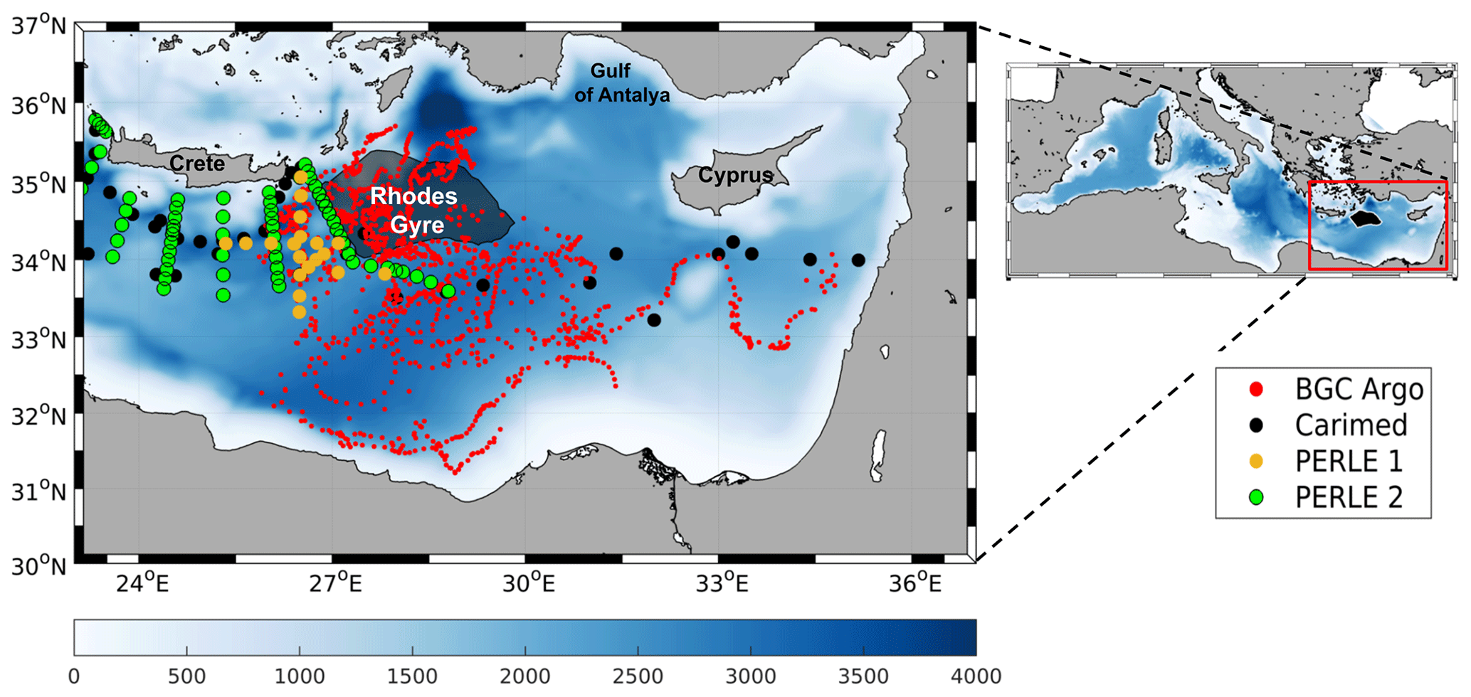
Figure 1 Model domain (right) and bathymetry (m) in the Mediterranean Sea and Levantine Basin. Red, black, yellow, and green dots indicate positions of Biogeochemical-Argo floats, CARIMED (CARbon, tracer and ancillary data In the MEDsea), PERLE-1, and PERLE-2 cruise data, respectively, from 2013 to 2020. The gray/black patch represents the Rhodes Gyre.

The Levantine Basin, in the southeastern Mediterranean Sea (Fig. 1), is a concentration basin, i.e., there is a net loss of water by evaporation, balanced by an input of less salty water from the Atlantic Ocean flowing successively through the straits of Gibraltar and Sicily (Lascaratos et al., 1993). The Levantine Basin is also a warm and salty sea, with surface temperatures reaching 27.9 ^∘C (El-Geziry, 2021) and salinity above 39.5 (Manca et al., 2004). Located in the northeastern part of the Levantine Basin, the Rhodes Gyre (Fig. 1) is a cyclonic persistent feature (Robinson et al., 2001; Millot and Taupier-Letage, 2005; Estournel et al., 2021), whose hydrodynamics have been well described in the literature, in particular following the POEM (Physical Oceanography of the Eastern Mediterranean) program in the 90s (Theocharis et al., 1993; Özsoy et al., 1991; 1993; Marullo et al., 2003). During cold winter wind events, the high-saline surface waters of the cyclonic Rhodes Gyre cool down, and their density increases, which generates deep mixing layers. During the following months, the newly formed dense water sinks to reach intermediate depths (130–400 m), forming the Levantine Intermediate Water (LIW, Hecht et al., 1988; Taillandier et al., 2022). Other studies have also reported LIW formations in the Gulf of Antalya (Sur et al., 1992; Kubin et al., 2019; Fach et al., 2021), in the southeastern margins of the basin, along the continental margins of the totality of the Levantine Basin (Brenner et al., 1991; Lascaratos et al., 1993; Özsoy et al., 1993), or in the Cretan Sea (Georgopoulos et al., 1989; Roether et al., 1998; Taillandier et al., 2022). However, the Rhodes Gyre remains the major area of LIW formation in the Levantine Basin (Lascaratos et al., 1999; Özsoy et al., 1989).

From a biogeochemical point of view, the eastern Mediterranean is a singular basin in terms of its oligotrophic to ultra-oligotrophic regimes (Krom et al., 1991; Siokou-Frangou et al., 2010; Pujo-Pay et al., 2011; Kress et al., 2014), with chlorophyll concentrations reaching at most 0.5 mg m⁻³ in the deep chlorophyll maximum layer (Mignot et al., 2014). Considered an “oasis” in the Levantine Basin (Siokou-Frangou et al., 1999), the Rhodes Gyre is characterized by higher phytoplankton biomass and biological production than the surrounding region (Vidussi et al., 2011). Yilmaz and Tugrul (1998) detailed the coupling of hydrodynamic conditions and nutrient enrichment in the gyre. Under prolonged and cold winter conditions, the Rhodes Gyre presents chimney formations, where Levantine deep or intermediate water, moving to the surface due to mixing, enriches the euphotic layer in nutrients (Yilmaz and Tugrul, 1998; Ediger and Yilmaz, 1996). Observational studies also showed that cyclonic features of the Rhodes Gyre determine the depth and thickness of the nutricline (Yilmaz et al., 1994). Ediger and Yilmaz (1996) highlighted the interannual variability in nutrient supply into the euphotic layer in the area, with fewer injections during mild winters compared to cold winters. This was in agreement with the one-dimensional coupled physical–biological modeling study by Napolitano et al. (2000), who found an increase of nutrient supply with the intensification of winter cooling across the same year. They also showed that the vertical extent of mixing influences the magnitude and timing of the spring phytoplankton bloom. Based on an analysis of ocean color satellite data, D'Ortenzio and Ribera d'Alcalà (2009) classified the Rhodes Gyre as a trophic regime with an intermittent phytoplankton bloom. They reported a strong interannual variability in the spatial shape and timing of the bloom. Mayot et al. (2016) further showed the alternation between bloom, intermittent, and no bloom regimes in the gyre.

After its formation, LIW spreads throughout the whole eastern Mediterranean Sea (Theocharis et al., 1993; Millot and Taupier-Letage, 2005; Estournel et al., 2021) and then heads towards the western Mediterranean and represents the main contribution to the outflow at the Strait of Gibraltar (Tanhua et al., 2013; Malanotte-Rizzoli et al., 2014). LIW is considered to play an important role in the formation of the Mediterranean intermediate and deep waters in the Aegean Sea, as well as in the southern Adriatic Sea and the northwestern Mediterranean Sea (Grignon et al., 2010; Velaoras et al., 2014; Margirier et al., 2020; Taillandier et al., 2022). This water mass may also have a critical impact on the biogeochemistry of the entire Mediterranean Sea (Astraldi et al., 1999; Malanotte-Rizzoli et al., 2014; Kress et al., 2014; Touratier and Goyet, 2009; Palmiéri et al., 2018). Thus, understanding its formation and propagation is a key to studying its impact on biogeochemical dynamics, first in the ultra-oligotrophic Levantine Basin and then in the entire Mediterranean Sea.

In spite of the importance of LIW in the hydrodynamics and biogeochemistry of the eastern and western Mediterranean Sea, relatively few studies have been conducted since the POEM program in the 90s (The POEM group, 1992), partly because of the complex geopolitical situation and restricted access. In particular, in situ cruise data remain rare in the Rhodes Gyre (Napolitano et al., 2000; Marullo et al., 2003), with most studies having been conducted in the northeastern Levantine Basin (Krom et al., 2005; Hassoun et al., 2019; Alkalay et al., 2020; Fach et al., 2021) or through a limited section in the basin (Moutin and Raimbault, 2002; Pujo-Pay et al., 2011; Santinelli, 2015) and mostly during the stratification period. On the other hand, only one 1D coupled hydrodynamic–biogeochemical model has been carried out in the Rhodes Gyre (Napolitano et al., 2000), while most 3D modeling studies investigated the whole Mediterranean Sea (Lazzari et al., 2012; Macias et al., 2014; Guyennon et al., 2015; Richon et al., 2017, 2018; Kalaroni et al., 2020; Cossarini et al., 2021) or eastern Mediterranean Sea (Petihakis et al., 2009) without focusing on the LIW formation region of the Rhodes Gyre.

Along with the deployment of Argo floats in the Levantine Sea since 2015 (Pasqueron de Fommervault et al., 2015), the PERLE (Pelagic Ecosystem Response to deep water formation in the Levant Experiment) project, within the framework of which this study takes place, was conducted in order to obtain a better understanding of the formation and spreading of LIW and their impacts on the distribution of nutrients and planktonic ecosystems. In the frame of the PERLE project, D'Ortenzio et al. (2021) documented, using Biogeochemical-Argo floats and in situ data sampled during the cruise, a coupling between mixed layer and phytoplankton dynamics in the Rhodes Gyre. They found that winter deepening of the mixed layer induces a steady injection of nitrate into the surface, followed by a rapid accumulation of phytoplanktonic biomass. However, this study is limited to parameters measured by biogeochemical floats, which does not allow for a more detailed exploration of biogeochemical and ecosystem dynamics. Furthermore, the intermittent trophic status of the area suggests significant interannual variability that remains poorly understood. In order to fill these gaps, the present study aims to gain insight into carbon dynamics through the examination of seasonal and interannual variabilities of the biogeochemical and physical fluxes of organic carbon, under particulate and dissolved forms, in the Rhodes Gyre and the estimate of an annual budget of organic carbon in the area over a multi-annual period. For that, we analyzed a simulation of a 3D hydrodynamic–biogeochemical coupled model implemented over the Mediterranean Sea over the period from December 2013–April 2021, and we focused on the Rhodes Gyre. The paper is organized as follows: first we describe in Sect. 2 the numerical models and the various data sets used to evaluate the model. Then, in Sect. 3 we present the assessment of the coupled model, the seasonal and interannual physical and biogeochemical variability, and an annual budget of organic carbon. Results are discussed in Sect. 4, and conclusions are given in Sect. 5.

2 Material and methods

2.1 The coupled physical–biogeochemical model

2.1.1 The hydrodynamic model

The 3D primitive equation ocean model SYMPHONIE is described in detail in Marsaleix et al. (2006, 2008), Estournel et al. (2016), and Damien et al. (2017). This model has primarily been used to describe the circulation in response to wind forcing and the dynamics of river plumes (Estournel et al., 1997, 2001; Marsaleix et al., 1998), coastal circulations (Estournel et al., 2003; Petrenko et al., 2008), dense water formation (Estournel et al., 2005; Ulses et al., 2008; Herrmann et al., 2008; Estournel et al., 2016), and shelf-slope exchanges (Mikolajczak et al., 2020).

2.1.2 The biogeochemical model

Eco3M-S is a biogeochemical multi-nutrient and multi-plankton functional type model, representing the dynamics of the pelagic planktonic ecosystem previously described by Auger et al. (2011) and Ulses et al. (2021). It describes the cycles of carbon (C), nitrogen (N), phosphorus (P), silicon (Si), dissolved oxygen (O₂), and chlorophyll (Chl). The model is composed of eight compartments: dissolved inorganic nutrients (nitrate, ammonium, phosphate, and silicate), dissolved oxygen, phytoplankton represented by three size classes (pico-, nano-, and micro-phytoplankton), zooplankton formed of three size classes (nano-, micro-, and meso-zooplankton), bacteria, particulate organic matter (POM), divided into two groups based on their settling speed (fast and slow settling speed), and dissolved organic matter (DOM). A summary diagram of the food web structure of the model and the interactions between the compartments is represented in Fig. S1 in the Supplement.

The model was previously used in the Mediterranean Sea to study the pelagic ecosystem and biogeochemical processes in coastal areas (Auger et al., 2011; Many et al., 2021) and open-sea regions (Herrmann et al., 2013; Auger et al., 2014; Kessouri, 2015, 2017, 2018; Ulses et al., 2016, 2021).

2.1.3 Implementation

The model configuration and implementation of the hydrodynamic simulation were described by Estournel et al. (2021). The model domain covers the Mediterranean Sea as well as the Marmara Sea and reaches 8^∘ west in the Gulf of Cádiz. The horizontal grid is characterized by a resolution that varies between 2.3 and 4.5 km from the northwest to the southeast to account for the increase of the Rossby deformation radius, therefore allowing an adequate representation of mesoscale processes. As for the Gibraltar Strait, the model resolution was further increased to a 1.3 km grid for a better representation of the exchange area between the Mediterranean Sea and Atlantic Ocean. The vertical grid uses a VQS (vanishing quasi sigma) coordinate system with 60 levels and increased resolution near the surface. This model configuration was used to describe the surface and intermediate water circulations in the eastern Mediterranean Sea (Estournel et al., 2021). The SYMPHONIE simulation is performed from 1 July 2011 to 2 May 2021. The meteorological parameters (with radiative fluxes) are hourly operational forecasts based on ECMWF 12 h analyses at $\mathrm{1}/\mathrm{8}$^∘ horizontal resolution. A total of 142 rivers (Fig. S2 in the Supplement) are considered in the model. As for the rivers of the Levantine Basin, the monthly climatology discharges were based on the study of Poulos et al. (1997), except for the Nile River where the discharge value was set to 475 m³ s⁻¹, following Nixon (2003).

We used the daily 3D current velocity, temperature, salinity, and vertical diffusivity outputs of the hydrodynamic simulations as forcing fields for the biogeochemical model run on the same grid. The biogeochemical model runs for the period from 15 August 2011 to 2 May 2021, but outputs are analyzed from December 2013. The time step is 20 min for advection and diffusion of biogeochemical variables and 2 h for biogeochemical reactions. We initialized the biogeochemical model with observation profiles during the stratified period averaged over 10 regions of the Mediterranean Sea (indicated in Fig. S2). For inorganic nutrient profiles, we used the CARIMED (CARbon, tracer and ancillary data In the MEDsea) database (Àlvarez et al., 2019; see Sect. 2.2.2), considering only summer data over the period 2011–2012, when data were available. Due to the lack of summer observations for the Levantine region, we used spring observations over the same period. Regarding the dissolved oxygen and chlorophyll concentrations, we initialized using summer in situ observations from Biogeochemical-Argo floats (BGC-Argo, Argo, 2022) (see Sect. 2.2.3) and the CARIMED database. Solar radiation and wind forcing for the biogeochemical simulation are those used for the hydrodynamic simulation. Atmospheric depositions of inorganic nutrients were taken into account. Nitrate and ammonium atmospheric depositions were applied as constant values based on the results of Kanakidou et al. (2012), Ribera d'Alcala et al. (2003), Powley et al. (2017), and Richon et al. (2018), and silicate deposition was prescribed as constant values for western (west of the Sicily Strait) and eastern basins based on estimates given by Ribera d'Alcalà et al. (2003). We deduced phosphate deposition from monthly Saharan dust deposition modeled with the regional model Aladdin Climate (Nabat et al., 2015) and averaged over the period 1979–2016. We hypothesized that phosphorus represents 0.07 % of dust and that 15 % is in soluble form (Herut and Krom, 1996; Guerzoni et al., 1999; Ridame and Guieu, 2002; Richon et al., 2017). Nutrient fluxes at the water column and/or sediment interface have been obtained through a coupling of the biogeochemical model with a simplified version of the vertically integrated benthic model described by Soetaert et al. (2000). At the river mouths, concentrations of nutrients were imposed using the results of Ludwig et al. (2010), who estimated the nutrient river discharge for the main rivers and 10 sub-regions of the Mediterranean Sea (Alboran, southwestern, northwestern, Tyrrhenian, Adriatic, Ionian, central, Aegean, north Levantine, south levantine). In the Atlantic Ocean, nutrients were prescribed using monthly profiles from the World Ocean Atlas 2009 climatology (https://odv.awi.de/en/data/ocean/world-ocean-atlas-2009/, last access: 16 April 2022) at 5.5^∘ W. In the Marmara Sea, in order to represent a two-layer flow regime, we imposed a relaxation with a timescale of 1 d towards nitrate concentrations of 0.24 and 1.03 mmol N m⁻³ and phosphate concentrations of 0.06 and 0.05 mmol P m⁻³ for depths above and below 15 m, respectively, based on the observations near the Dardanelles Strait from Tugrul et al. (2002).

2.1.4 Definition of the study area and budget calculation

In this paper, the analysis of the simulation of the whole Mediterranean basin is restricted to the Rhodes Gyre. Previous studies determined the Rhodes Gyre's location based on a sea surface temperature (SST) criteria. Marullo et al. (2003) using AVHRR (Advanced Very High Resolution Radiometer) images time series located the gyre in an area between the southeast of Rhodes and the east of Crete: 34–36^∘ N and 27–30^∘ E with a threshold of 14 ^∘C. D'Ortenzio et al. (2021) identified the region using a SST threshold at 15 ^∘C based on satellite images. Other studies have also used the sea surface height (SSH) from ADT (absolute dynamical topography) maps to detect mesoscale features of the Mediterranean Sea such as Cornec et al. (2021).

In this study, we defined the Rhodes Gyre area based on modeled surface density. The winter mean surface density was calculated between January and mid-March, the period generally associated with deep vertical mixing (Malanotte-Rizzoli et al., 2003). The Rhodes Gyre was defined by the area where the density anomaly is above 28.8 kg m⁻³. The resulting region (indicated in Figs. S3 in the Supplement and Fig. 1 in the article) designates a large area of the Rhodes Gyre, covering 27 500 km², that includes areas where the strongest mixing occurred over the period 2014–2021 (Fig. S3). The hydrodynamic and the biogeochemical variables presented in the following sections correspond to values averaged over this domain.

To calculate the organic carbon budget, the water column was divided into two layers. The surface layer is defined as the euphotic layer, covering the surface to 150 m of depth, and the intermediate layer is from 150 to 400 m, which includes the LIW (Ozer et al., 2016; Menna and Poulain, 2010, 2021). Organic carbon englobes dissolved and particulate organic carbon (DOC and POC, respectively). The latter includes all modeled components of POC: low and fast sinking detritic particles and living organisms, i.e., the three size classes of phytoplankton, the three size classes of zooplankton, and bacteria. The biogeochemical contribution to the organic carbon budget is the sum of gross primary production (GPP) and organic carbon consumption through community respiration (CR) (phytoplankton, zooplankton, and bacteria respiration) (see Table S4 in Supplement Material by Many et al., 2021). The physical contribution of the budget is divided into two components: lateral transport and vertical transport, both due to mixing and advection. Lateral transport represents the net transport at the lateral limits of the Rhodes Gyre area. Vertical transport represents the exchanges at the vertical boundaries of the layer. Positive values correspond to fluxes of organic carbon that enters the considered layer of the Rhodes Gyre area. Similarly, negative values correspond to fluxes of organic carbon that leaves the considered layer of the Rhodes Gyre area. The variation of organic carbon inventory, the biological term, and the lateral physical term were calculated online, i.e., during the simulation, while the vertical term was calculated as the residual based on values of all other terms. The equations of the budget are given in the Supplement material (Text S1 in the Supplement).

2.2 Observations used for the coupled model assessment

In order to assess the performance of the model, we used remote sensing, in situ, and BGC-Argo float data over the study period. Because the number of observations in the Rhodes Gyre area is limited, the comparison was conducted all over the Levantine Basin. The spatial coverage of the in situ data set used in this study is shown in Fig. 1.

2.2.1 Satellite data

To evaluate the modeled surface chlorophyll concentration, we used daily level 4 reprocessed data obtained from the European Copernicus Marine Environment Monitoring Service (CMEMS) from the website (http://resources.marine.copernicus.eu/, last access: 16 June 2022, products: OCEANCOLOUR_MED_CHL_L4_REP_OBSERVATIONS_009_078, last access: 16 June 2022), with a spatial resolution of 1 km. The latter is a regional product with daily interpolated chlorophyll concentrations from multi sensors (MODIS-Aqua, NOAA-20-VIIRS, NPP-VIIRS, MERIS sensors). To compare model results with those data, we interpolated the data on the model grid.

2.2.2 Cruise observations

We used the CARIMED (CARbon, tracer and ancillary data In the MEDsea) database with 862 profiles covering cruise observations available in the Mediterranean Sea for the period 2011–2018 (Àlvarez et al., 2019) to complete the assessment of the spatial distribution of the simulated variables. The data passed two quality controls following the GLODAP (Global Ocean Data Analysis Project) procedure (Key et al., 2004) adapted to the Mediterranean Sea. This data set included cruises with only best-practiced standards for nutrients following the GO-SHIP (Global Ocean Ship-based Hydrographic Investigations Program) and the WOCE (World Ocean Circulation Experiment) protocols. Fourrier et al. (2020) added data from 10 other cruises to the data set and validated them. The data are available on figshare (https://doi.org/10.6084/m9.figshare.12452795.v2, last access: 10 October 2022, Fourrier, 2020). Sea water was collected using Niskin bottles from the surface to 4600 m of depth. An SBE 43 oxygen sensor was used during the cruises and adjusted with Winkler measurements. The inorganic nutrients were determined following the colorimetric methods of Grasshoff et al. (1999).

In addition, we also used the PERLE cruise data set: PERLE-1 (25 profiles) covering the Levantine Basin in October 2018 and PERLE-2 (29 profiles) in February–March 2019 (D'Ortenzio et al., 2021). At all stations, water samples were collected from Niskin bottles for nutrient analysis. This data set passed a primary quality control.

It is important to mention that we used validation data different from calibration data to prevent overfitting of model parameters and to have a better assessment of the model's reaction capacity when the validation patterns are different from those used in the calibration; this method was supported by Robson (2014).

2.2.3 BGC-Argo floats

To evaluate the temporal and the spatial variability of the modeled dissolved oxygen and chlorophyll, we used observations from BGC-Argo floats providing O₂ (1566 profiles) and Chl a (1171 profiles) measurements (Argo, 2022) deployed in the eastern Mediterranean, downloaded from the Argo Global Data Assembly Center web portal, accessible through the Coriolis database (http://www.coriolis.eu.org, last access: 21 June 2022). Regarding O₂ measurements made by Argo floats, air measurements and optode calibration protocols have led to a significant improvement in the quality and accuracy of these data (Bittig et al., 2018; Bittig and Körtzinger, 2015). These can now reach accuracies of 1–1.5 µmol kg⁻¹ close to those achieved in situ by the Winkler method. Mignot et al. (2019) conducted a similar study to try to quantify the observational errors for dissolved oxygen and chlorophyll concentrations. They found a bias of 2.9 ± 5.5 µmol kg⁻¹ and −0.06 ± 0.02 mg m⁻³ for the oxygen and the chlorophyll, respectively, and a relative root mean square difference (RMSD) of 6.1 % for oxygen and 5.4 % for chlorophyll in the Mediterranean Sea.

3 Results

3.1 Assessment of the coupled physical–biogeochemical model

The hydrodynamical model was evaluated by Estournel et al. (2021) by computing model/observation statistics using salinity and temperature observations from Argo floats and satellite data. The authors showed the ability of the model to reproduce the hydrological characteristics of the surface and intermediate waters in the eastern Mediterranean Sea. In the following section, we focus on the evaluation of the biogeochemical model in the Levantine Sea.

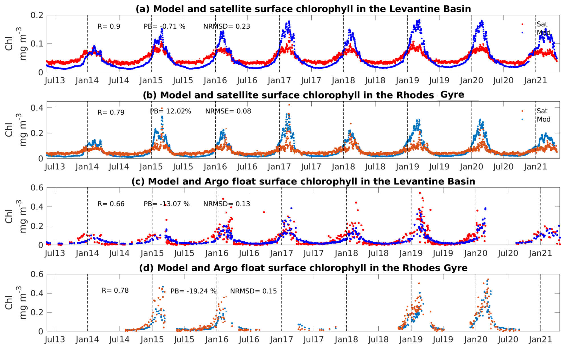
Figure 2 Time series of modeled (in blue) and satellite (in red) surface chlorophyll a concentration (mg m⁻³), averaged over (a) the Levantine Basin and (b) the Rhodes Gyre. Time series of modeled (in blue) and BGC-Argo float (in red) surface chlorophyll a concentration (mg m⁻³) (c) in the Levantine Basin and (d) in the Rhodes Gyre. Coefficient correlation (R), percent bias (PB), and normalized root mean square deviation (NRMSD) between model outputs and observations are indicated in panels (a–d).

3.1.1 Surface chlorophyll concentration

Figure 2 shows the temporal variation of the satellite and modeled surface chlorophyll averaged over the entire Levantine Sea (Fig. 2a), as well as the BGC-Argo float data and the modeled surface chlorophyll along the trajectory of floats located in the Levantine Sea (Fig. 2c and b, data located specifically in the Rhodes Gyre are indicated in lighter colors in Fig. 2b and d), over the study period. To quantify the differences between model outputs and observations, we calculated the percent bias (PB, 100 × $\frac{\mathrm{Meanmod}-\mathrm{Meanobs}}{\mathrm{Meanobs}}$, where Meanmod and Meanobs are the mean of the model outputs and observations, respectively) and the normalized root mean square difference (NRMSD $\sqrt{\frac{{\sum }_{k=\mathrm{1}}^k(\mathrm{Obs}-\mathrm{Mod}{)}^{\mathrm{2}}}{\mathrm{Maxobs}-\mathrm{Minobs}}}$, where Obs and Mod are the observation and model output, respectively; Maxobs and Minobs are the maximum and minimum observation values for the chlorophyll).

The model captures the seasonal dynamics of the observed satellite chlorophyll over the Levantine Basin (Fig. 2a) and more particularly in the Rhodes Gyre (Fig. 2b). At the end of fall, the chlorophyll concentration begins to increase progressively and reaches its maximum in February/March, with higher maxima in the Rhodes Gyre compared to the surrounding Levantine Sea in both the data and the model. The surface concentration is minimal in summer, for both the model and satellite. The model and satellite show differences in magnitude: in the model the winter maximum is generally higher, and the summer minimum values are lower, compared to the satellite data for both regions. The standard deviation (SD) of the model in the Levantine Basin (0.04 mg Chl m⁻³) and the Rhodes Gyre (0.07 mg Chl m⁻³) is close to the mean chlorophyll concentration (0.05 and 0.06 mg Chl m⁻³, respectively), which underlines the high variability of this oligotrophic system. The mean surface chlorophyll concentration in the satellite data for the Levantine Basin and the Rhodes Gyre is 0.05 ± 0.02 and 0.06 ± 0.02 mg Chl m⁻³, respectively. We obtain a highly significant correlation coefficient equal to 0.90 and 0.79 (p value < 0.01), and low values for the NRMSD (an error of 23 % and 8 %) and percent bias (−0.71, 12 %), between model outputs and satellite data over the whole study period for the Levantine Basin and the Rhodes Gyre, respectively.

Regarding the comparison with BGC-Argo float data in the Levantine Sea (Fig. 2c) and the Rhodes Gyre (Fig. 2d), the model correctly reproduces both the seasonal cycle and the magnitude of chlorophyll during the different periods of the year. Both model and float data show high variability in late winter/early spring in the Rhodes Gyre in agreement with previous studies (D'Ortenzio and Ribera d'Alcalà, 2009; Salgado-Hernanz et al., 2019; Kotta and Kitsiou, 2019). The statistical metrics show a significant correlation equal to 0.66 (p value < 0.01) between the observed and modeled values in the Levantine Sea. The NRMSD is equal to 13 %, and the percent bias remains low (−13 %). Similar statistical scores were obtained between the model outputs and the float data in the Rhodes Gyre, i.e., correlation (0.78, p value < 0.01) as well as low bias (−19 %) and NRMSD (15 %). The difference between the comparisons of model results with satellite data and those with BGC-Argo float data could be attributed in part to an underestimation of satellite chlorophyll concentration during winter in the Levantine Sea, as suggested by Vidussi et al. (2001) and reported by D'Ortenzio et al. (2021).

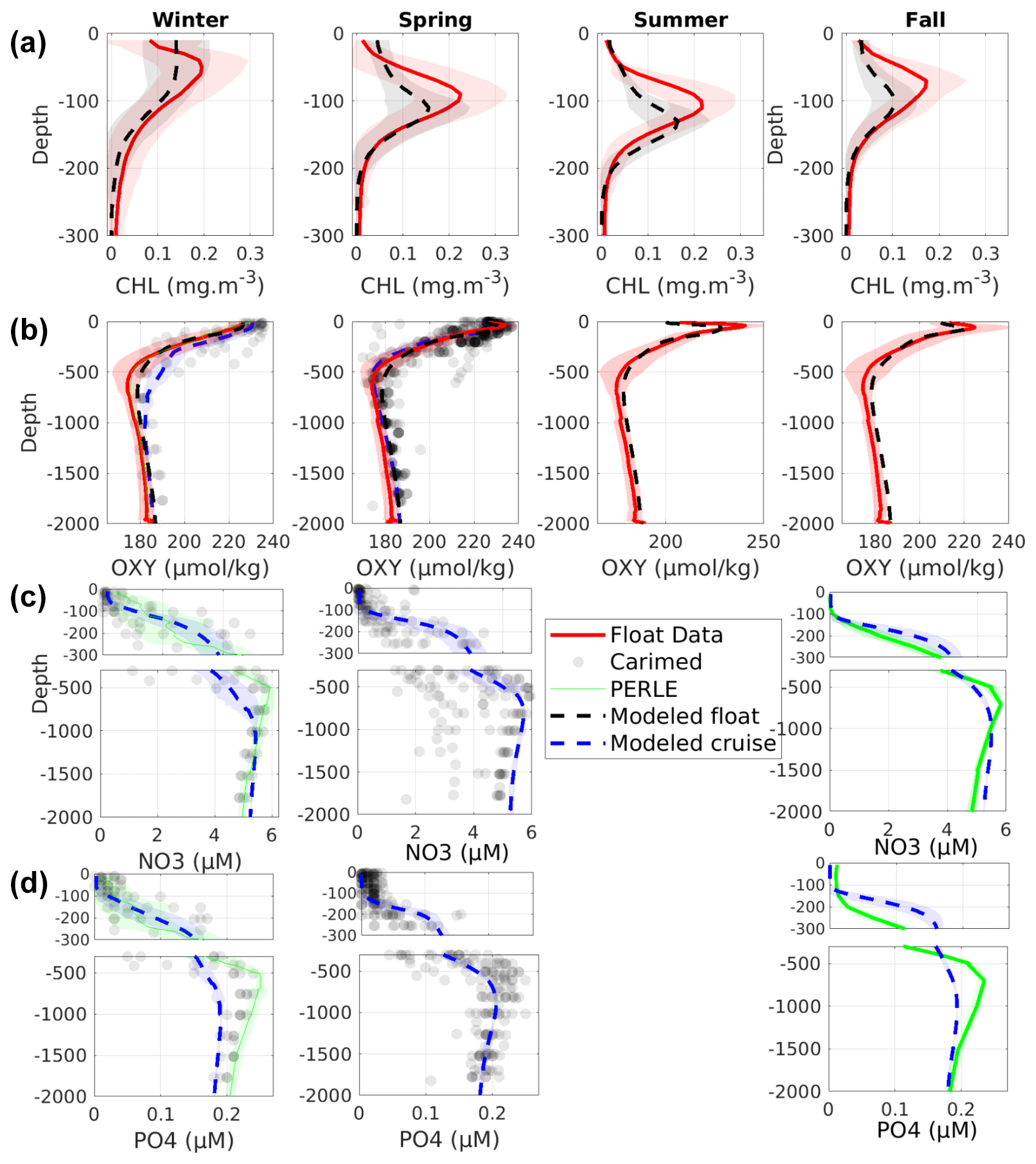
Figure 3 Comparison over the Levantine Sea between observed (gray points for CARIMED, green lines for PERLE-1 and PERLE-2, red line for BGC-Argo float data) and modeled (blue and black lines) profiles of chlorophyll (mg Chl m⁻³), dissolved oxygen (µmol kg⁻¹), nitrate (µM), and phosphate (µM) concentrations, averaged by season (winter: 21 December to 20 March, spring: 21 March to 20 June, summer: 21 June to 20 September, fall: 21 September to 20 December). Shaded areas represent standard deviation.

3.1.2 Seasonal variation of vertical distribution

Figure 3 shows a comparison of modeled and observed mean seasonal profiles of chlorophyll, dissolved oxygen, nitrate, and phosphate in the Levantine Sea from both BGC-Argo floats and the oceanographic cruises. The model results are compared with the observations at the same dates and positions. This comparison is completed by a statistical analysis computed over the whole period of study (Fig. S4 in the Supplement).

The model reproduces the development of a deep chlorophyll maximum (DCM) in spring and its presence in summer and fall, reaching a maximal depth in summer (Fig. 3a). During winter, the model overestimates the surface chlorophyll by 0.05 mg Chl m⁻³ and homogenization in the first 50 m. It generally underestimates the DCM concentration by 25 % and overestimates its depth by 20 m (130 and 110 m for the model and the float, respectively).

The magnitude and seasonal variation of the vertical profile of dissolved oxygen concentration are well reproduced (Fig. 3b). As with chlorophyll, the surface oxygen concentration is maximum during winter. It reaches 230 and 240 µmol kg⁻¹ for the model and the float data, respectively. The model reproduces the presence of a subsurface oxygen maximum in spring, summer, and fall, between 40 and 60 m depth as observed, with an underestimation of its concentration by 10 µmol kg⁻¹. The oxygen minimum layer concentration stands within the range of the observed values. The model is highly correlated with the different data sets (R > 0.95, p value < 0.01). The observations show a SD close to 16.5 µmol kg⁻¹ for the floats. The modeled float oxygen concentrations also show a high SD of ∼ 14.5 µmol kg⁻¹.

The model reproduces the general features of the nitrate and phosphate concentration profiles with an increase from the surface to 500–1000 m and a gradual, slow decrease below, close to those of the profiles imposed at the initialization, showing a stability over the simulation period (Fig. 3c and d). The modeled phosphate concentrations in the transitional layer (500–1000), located between the intermediate and deep layers, are in the lower-range values of observations. The surface nutrient profiles show low concentrations from the surface to 50 m during winter, while in spring and fall the layer depleted in nutrients reaches 100 m in both observations and model outputs.

The statistical analysis (Fig. S4) shows that the model displays high correlation (R > 0.90, p value < 0.01, for all the cruise data sets) and low RMSD (∼ 0.01, 0.03, and 0.02 mmol P m⁻³ for CARIMED, PERLE-1, and PERLE-2, respectively) and bias (0.006, −0.01, and −0.03 mmol P m⁻³ for CARIMED, PERLE-1, and PERLE-2, respectively) compared to the phosphate observations. PERLE-1 and PERLE-2 phosphate observations show high variability, with an SD ∼ 0.065 and 0.062 mmol P m⁻³, respectively. The modeled SD for both cruises is slightly smaller in comparison with observations (0.050 and 0.040 mmol P m⁻³). As for nitrate, the metrics confirm the good agreement between model outputs and observations, with significant correlations above 0.95 (p value < 0.01); a bias of 0.1, −0.1, and 1.4 mmol N m⁻³ for PERLE-1, PERLE-2, and CARIMED, respectively; and a RMSD close to 0.4 mmol N m⁻³ for PERLE-1 and PERLE-2 and 1.3 mmol N m⁻³for CARIMED.

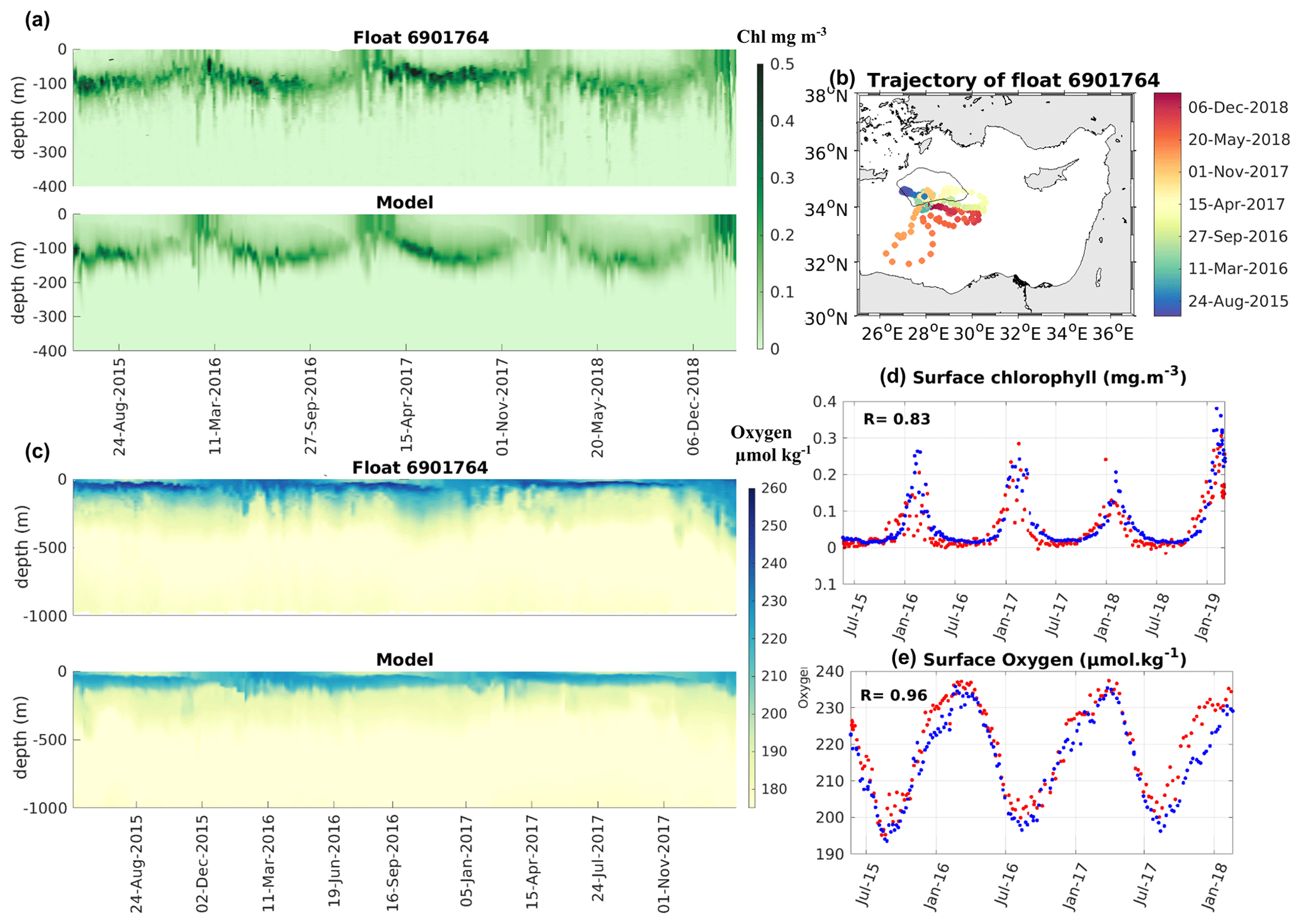
Figure 4 Time evolution of BGC-Argo float 6901764 observed and modeled data: (a) Hovmöller diagrams of chlorophyll concentration (mg m⁻³), (b) trajectory of the BGC-Argo float (the black line indicates the limit of the defined Rhodes Gyre area), (c) Hovmöller diagrams of dissolved oxygen concentration (µmol kg⁻¹), (d) surface chlorophyll (mg m⁻³) in the first 10 m, and (e) surface dissolved oxygen (µmol kg⁻¹) observed in the first 10 m. Red dots represent the float data and the blue dots the model outputs in panels (d) and (e).

3.1.3 Case study: BGC-Argo float/model comparison

Figure 4 represents the evolution of the chlorophyll and oxygen concentrations for float 6901764 and those extracted from the model at the same time and location (both indicated on Fig. 4b). The choice of the float was done based on both the temporal extension and the localization of the platform: this float covers both the Rhodes Gyre and the surrounding region for a long period, 2015–2019 (Fig. 4b). The model reproduces the observed seasonal cycle, with an increase in the surface chlorophyll during winter (Fig. 4d) followed by the formation and deepening of the DCM (Fig. 4a). The DCM is mostly well localized in the model (10–20 m deeper than in the observations during summer). The model accurately reproduces the vertical distribution of chlorophyll, although some differences exist, such as the slight underestimation of the intensity of the maximum chlorophyll also noted in Fig. 3. The surface chlorophyll concentrations for the first 10 m from the simulation and the float data (Fig. 4d) are significantly correlated (R = 0.83, p value < 0.01).

The modeled and observed oxygens display a similar seasonal cycle, with an increase in surface oxygen concentration during winter (Fig. 4e) followed by a decrease at the surface and a deepening of the oxygen maximum (Fig. 4c) during the stratification period. In both the model outputs and observations, the oxygen minimum layer is located at depths between 300 and 1000 m. The model and the float show a good temporal correlation for the surface concentration of dissolved oxygen (R = 0.96, p value < 0.01, Fig. 4e).

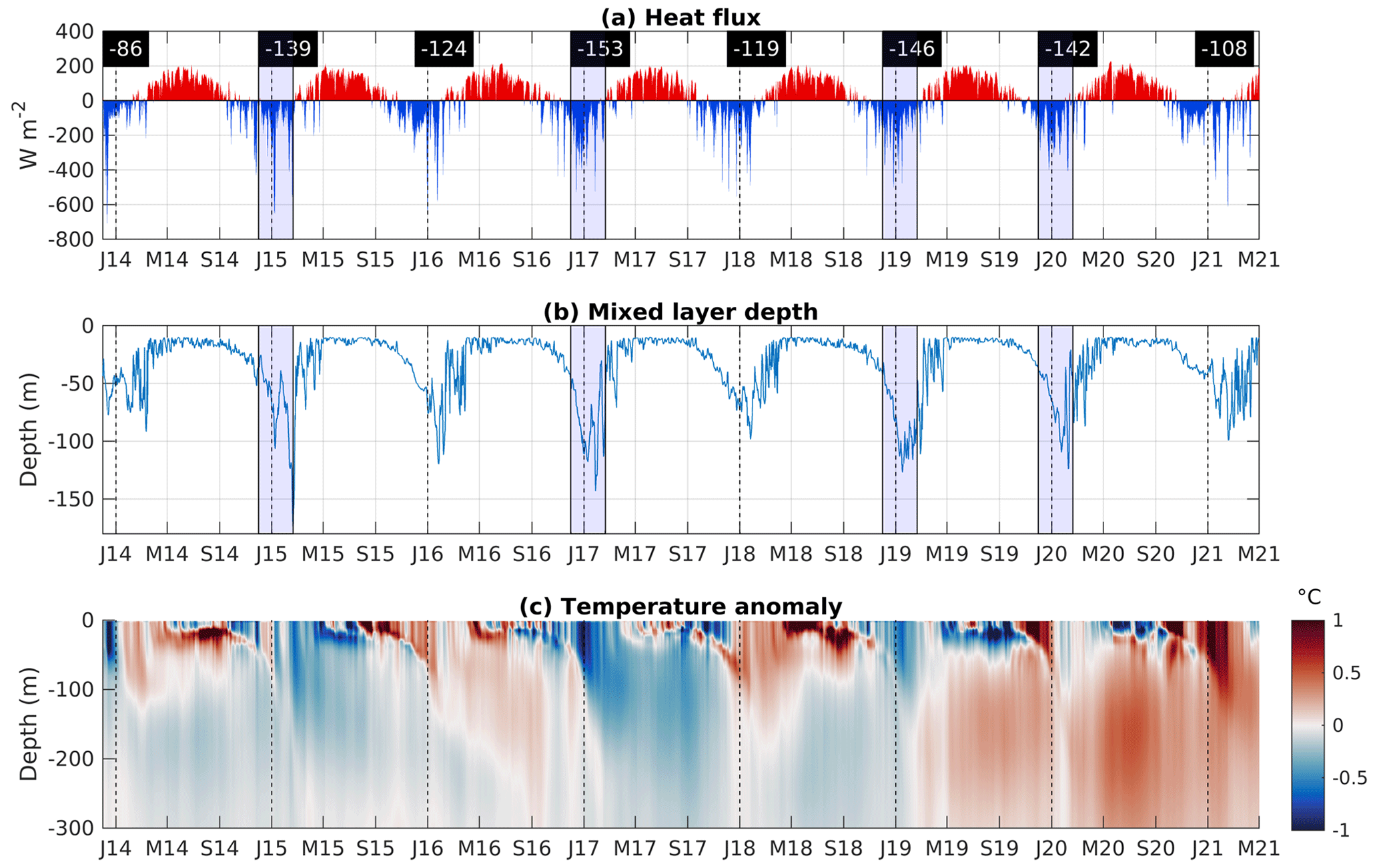
Figure 5 Time series of modeled (a) surface heat fluxes (W m⁻²), (b) mixed layer depth (m), and (c) temperature anomaly (^∘C), averaged over the Rhodes Gyre area. The winter (December–January–February) mean heat flux is indicated in black rectangles in panel (a). J: January, M: May, S: September. Winters with strong heat loss and deeper mixed layers are emphasized in blue in panels (a) and (b).

3.2 Meteorological and hydrodynamic variability

Figure 5 exhibits the time series of surface heat fluxes, mixed layer depth (MLD), and temperature profile anomaly (computed based on the difference in temperatures from the mean daily temperature over the 7 years), spatially averaged over the Rhodes Gyre area (defined in Sect. 2.1.4). The mixed layer depth is defined as the depth where the potential density exceeds by 0.01 kg m⁻³ its value at 10 m depth (Coppola et al., 2017). These density-based criteria are more appropriate than shallower temperature-based MLD estimates to represent mixing in the dense water formation zone, such as the Rhodes Gyre, as suggested by Houpert et al. (2015).

The domain displays a seasonal cycle, characterized by a heat loss at the air–sea interface from October to March followed by a heat gain from April to the end of September (Fig. 5a). During autumn, the strong heat losses, induced by cold northerly wind events (Horton et al., 1997), weaken the stratification and induce mixing until depths around 40–50 m (Fig. 5b). The following northerly wind/heat loss events in winter further favor the deepening of the mixed layer, with the maximum depth ranging between 90 and 180 m in February/March. After March, the sea gains heat, restratifying the surface layer, and the MLD abruptly decreases. The seasonal pattern of modeled heat flux and MLD is in agreement with the climatology of the heat storage rates reported by D'Ortenzio et al. (2005) and Houpert et al. (2015). The Rhodes Gyre area displays a minimum winter temperature, lower than 16.5 ^∘C, in the Levantine Basin (Fig. S5a in the Supplement).

A strong wintry interannual variability of surface heat flux, as well as of wind stress magnitude and MLD, is clearly visible (Figs. 5 and S6, Table S1 in the Supplement). Winters 2014–2015, 2016–2017, 2018–2019, and 2019–2020 are characterized by a winter mean heat loss higher than the 7-year winter average, i.e., 130 W m⁻² (Table S1, Fig. S6), and with mean winter mixed layer depth close to or higher than the 7-year mean mixed layer of 68 m (Table S1). Cold winters (2014–2015, 2018–2019, and 2019–2020) are also marked by strong winter wind stresses, except for 2016–2017, characterized by the highest winter heat loss (Fig. S6). Among the mild winters, winter 2013–2014 presents both a strong positive winter heat flux anomaly and a strong negative winter wind stress anomaly, as a consequence of the absence of cold winds from January onwards, leading to the shallowest mixed layers (Table S1). Negative anomalies of temperature are generally visible over the ML in winter and in the subsurface during the stratification period for years of high winter heat losses (2014–2015, 2016–2017, 2018–2019, and 2019–2020; Fig. 5c). These anomalies extend below the subsurface for the years 2014–2015 and 2016–2017, marked by deep winter mixing.

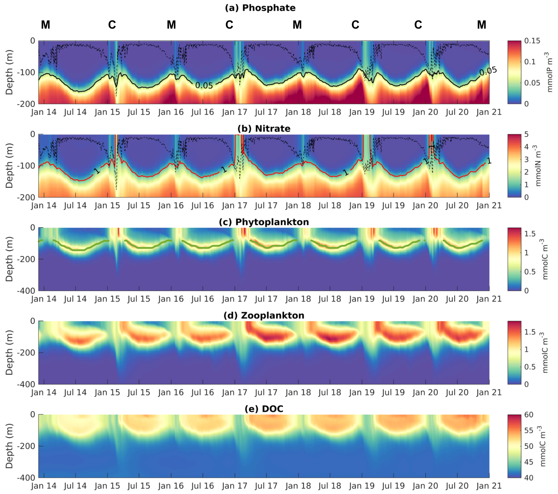
Figure 6 Hovmöller diagrams of modeled (a) phosphate (mmol P m⁻³), (b) nitrate (mmol N m⁻³), (c) phytoplankton (mmol C m⁻³), (d) zooplankton (mmol C m⁻³), and (e) dissolved organic carbon (mmol C m⁻³) concentrations averaged over the Rhodes Gyre, from December 2013 to January 2021. The dotted black line in panels (a) and (b) indicates the mixed layer depth. The red line represents the depth of the nitracline in panel (b) and the black one of the phosphacline in panel (a). The green line in (c) indicates the deep chlorophyll maximum. C refers to cold winter years and M to mild winter years.

3.3 Variability of the pelagic planktonic ecosystem

Figure 6 presents the modeled time series of vertical profiles of nutrients, phytoplankton, zooplankton, and dissolved organic carbon concentrations, spatially averaged over the Rhodes Gyre area.

During fall, nutrient concentrations gradually increase in the surface layer with the weakening of the stratification and the gradual rise of the nutricline (defined here as isoline 1 mmol N m⁻³ for nitracline and 0.05 mmol P m⁻³ for phosphacline) up to the surface (Figs. 6a, b and S7a–c in the Supplement), induced by the reduction of solar insolation and the shallowing of the DCM, possibly reinforced by the intensification of the cyclonic circulation. As for the DOC concentration, it starts decreasing gradually in the first 100 m in mid-fall with the weakening of the stratification (Figs. 6e and S7a, f).

During winter, surface phytoplankton concentration starts to increase when the mixed layer depth increases and persistently reaches the nutriclines (Figs. 6a–c and S7a–d). The Rhodes Gyre area is enriched in nutrients at the surface (Fig. S5c) and is characterized by surface maximum chlorophyll concentrations over the Levantine Sea (Fig. S5b). The zooplankton concentration generally begins to increase after the onset of the phytoplankton accumulation in winter (Figs. 6c, d and S7d, e). The DOC concentration in the 0–100 m layer further decreases during the winter mixing period, from January to March (Figs. 6e and S7f). One can also notice that the deepening of the mixed layer in winter is also responsible for the transfer of both plankton and DOC below 150 m, where their concentrations increase (Fig. 6c and e). The maximum surface concentration for phytoplankton reaches values higher than 0.5 mmol C m⁻³ between February and March (Fig. 6c, Table S1). Zooplankton concentration reaches its maximum (1–1.5 mmol C m⁻³) near the surface in March–April (Fig. 6d). Phytoplankton growth stops at the surface when it becomes depleted in phosphate, while the surface nitrate concentration ranges between 0.3 and 1 mmol N m⁻³ during winter, in agreement with the observations of Yilmaz and Tugrul (1998) (Fig. 6a–c). Then, the deep chlorophyll maximum (dotted green line in Fig. 6c) forms. The DOC concentration progressively increases during spring (Fig. 6e).

During summer, the depletion in nutrients increases and deepens: phosphate and nitrate concentrations in the first 150 m are lower than 0.01 mmol P m⁻³ and 0.1 mmol N m⁻³, respectively (Fig. 6a and b). The summer-averaged nitracline and phosphacline are localized at 131 and 144 m, respectively. The averaged DCM for all summer periods is at a mean depth of 128 m with magnitudes between 0.2 and 0.3 mg Chl m⁻³ (Fig. 6c). One should notice that the depth of DCM coincides with the depth of deep carbon maximum. Throughout the summer, the biomass of phytoplankton decreases. The decline of phytoplankton at the end of summer induces a zooplankton decrease (Fig. 6d). On the contrary, DOC accumulates due to stratification and reaches its maximum, ranging from 52 to 55 mmol C m⁻³, in early August (Fig. 6e).

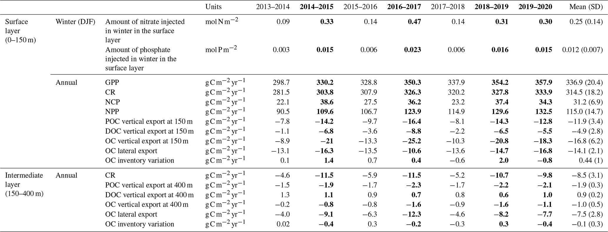
Table 1 Amount of nutrients injected into the surface layer in winter (December–January–February) in the Rhodes Gyre, annual biogeochemical carbon flows: gross and net primary production (GPP and NPP), net community production (NCP), community respiration (CR), downward export flux of particulate and dissolved organic carbon (POC and DOC), and the study area. The annual budget is calculated from December. Lateral export at 150 and 400 m for the different years and averaged over the 7-year period, estimated from the model. Positive values correspond to an input for the considered layer of the study area. Cold years are indicated in bold. The annual budget is calculated from December.

Interannual variability of nutrient and phytoplankton concentrations is strong during the mixing period when deep nutrients are injected into the surface layer (Figs. 6a, b and S7). During the cold winters (noted C in Fig. 6) of 2014–2015, 2016–2017, 2018–2019, and 2019–2020, the mixed layer reaches the nutriclines over a larger area (not shown) and period, allowing higher nutrient supplies into the surface layer (Table 1). The interplay between vertical mixing, deep nutrient injection, and increase in surface phytoplankton shows interannual variability, as illustrated in Fig. S8 in the Supplement, for the mild winter of 2013–2014 and the cold winter of 2014–2015. When the mixed layer punctually reaches the nutriclines in early winter or throughout a mild winter as in 2013–2014 (Fig. S8a), surface nutrients and chlorophyll increase gradually and nearly synchronously. When the winter is severe as in 2014–2015 (Fig. S8b), the surface nutrient response is a rapid increase each time (< 1 d see for example early January and early February 2015), while the chlorophyll response depends on the depth of the MLD. In the case that it is shallower than the euphotic layer, chlorophyll increases gradually (∼ 12 d in January 2015). In the case that the MLD exceeds the euphotic layer as in February 2015, chlorophyll development is delayed due to dilution of phytoplankton cells in the deep ML and light limitation for phytoplankton growth. As a consequence of higher nutrient injections, surface phytoplankton concentrations reach higher values (> 1.5 mmol C m⁻³ and 0.3 mg Chl m⁻³) during cold winters compared to mild winters (< 1 mmol C m⁻³ and 0.23 mg Chl m⁻³) (Table S1). These differentiated chlorophyll responses to the mixed layer described here as a function of time also appear simultaneously at different points in space. As an example, Fig. S9 in the Supplement shows a low chlorophyll concentration on 20 February 2015 in the core of the Rhodes Gyre, where vertical mixing is the most intense, and higher concentrations in the border of the gyre (Fig. S9a and c). Modeled surface chlorophyll averaged over the Rhodes Gyre area is then maximum 12 d later, on 4 March 2015, when it reaches higher concentrations in the center of the gyre as soon as the water column is restratified (Fig. S9b and d). With regard to the date of the maximum surface chlorophyll, no clear link with winter severity can be established. The former is instead related to the timing and history of wind events favoring the deepening of the ML, submitted to high interannual variability. For example, the chlorophyll maximum was found in mid-February during both the mild winter of 2015–2016 and the severe winter of 2016–2017, respectively (Table S1).

Regarding zooplankton, the spring surface concentration is minimal during the mild year of 2013–2014 and maximum during the cold years of 2016–2017, 2018–2019, and 2019–2020 (Fig. 6d). High concentrations are also visible along the DCM layer for those years, as well as in 2018. DOC concentrations show similar interannual variability to zooplankton (Fig. 6e).

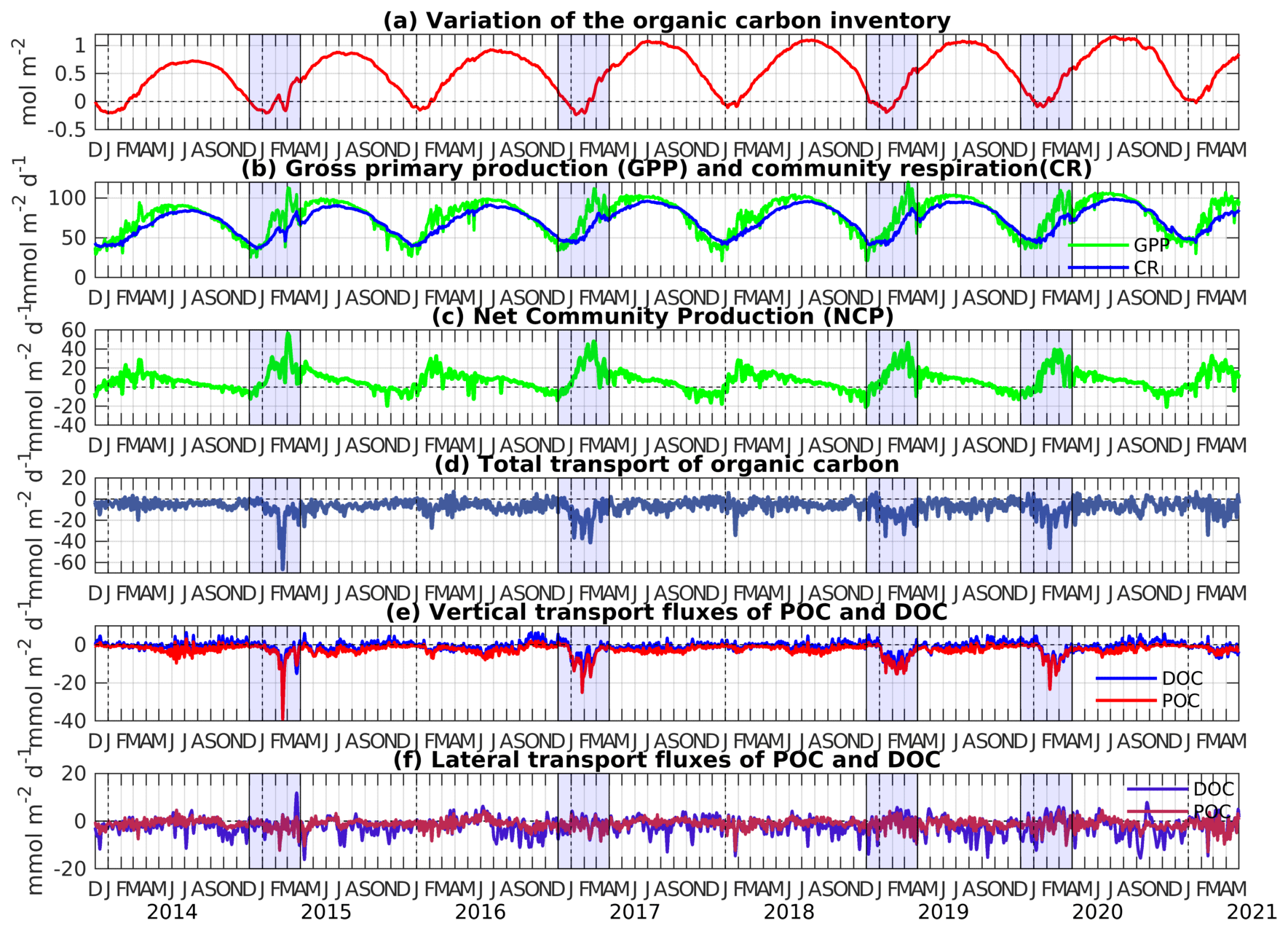
Figure 7 Time evolution of (a) the variation of the organic carbon inventory (from 1 December 2013, mol C m⁻²), (b) gross primary production (GPP) (in green) and community respiration (CR) in the surface layer (in blue) ($\mathrm{mmol}\mathrm{C}{\mathrm{m}}^{-\mathrm{2}}{\mathrm{d}}^{-\mathrm{1}}$), (c) net community production (NCP) ($\mathrm{mmol}\mathrm{C}{\mathrm{m}}^{-\mathrm{2}}{\mathrm{d}}^{-\mathrm{1}}$), (d) total transport of organic carbon at the limits of the area ($\mathrm{mmol}\mathrm{C}{\mathrm{m}}^{-\mathrm{2}}{\mathrm{d}}^{-\mathrm{1}}$), (e) vertical transport fluxes of POC and DOC at the base of the surface layer ($\mathrm{mmol}\mathrm{C}{\mathrm{m}}^{-\mathrm{2}}{\mathrm{d}}^{-\mathrm{1}}$), and (f) lateral transport fluxes of POC and DOC at the limits of the area ($\mathrm{mmol}\mathrm{C}{\mathrm{m}}^{-\mathrm{2}}{\mathrm{d}}^{-\mathrm{1}}$), averaged over the Rhodes Gyre surface layer (0–150 m). Cold winters/early springs are emphasized in blue.

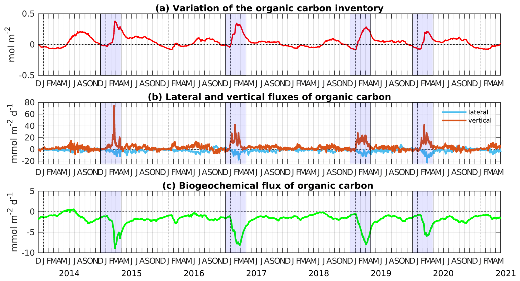
Figure 8 Time evolution of (a) the variation of the organic carbon inventory (from 1 December 2013, mol C m⁻²), (b) lateral and vertical transport fluxes of organic carbon ($\mathrm{mmol}\mathrm{C}{\mathrm{m}}^{-\mathrm{2}}{\mathrm{d}}^{-\mathrm{1}}$) at the limits of the area, and (c) biogeochemical flux of organic carbon ($\mathrm{mmol}\mathrm{C}{\mathrm{m}}^{-\mathrm{2}}{\mathrm{d}}^{-\mathrm{1}}$), averaged over the Rhodes Gyre intermediate layer (150–400 m). Cold winters/early springs are emphasized in blue.

3.4 Organic carbon inventory and fluxes

Figures 7 and 8 represent, respectively, in the surface (0–150 m) and intermediate (150–400 m) layers of the Rhodes Gyre area, the variability of the organic carbon inventory, the biogeochemical fluxes, and the vertical and horizontal exchanges at the limits of the two boxes. In the surface layer, the inventory of organic carbon is minimum in January and maximum in June/July (Fig. 7a). The modeled gross primary production (GPP) generally follows the cycle of the solar insolation (not shown), with minimum values in December and maximum values at the end of June. A secondary peak is visible between February and April (Fig. 7b). Its vertical distribution (not shown) is close to the one of phytoplankton (Fig. 6c) and mostly relies on recycled production (ammonium uptake represents 78 % of total nitrogen uptake). The community respiration (CR) follows a similar pattern to the GPP with a temporal shift of a few weeks. The resulting net community production (NCP, corresponding to GPP minus CR) shows a peak value in February/March, during the secondary peak in the GPP, and negative values from August to January (Fig. 7c), indicating that the region is autotrophic from January to April and heterotrophic for the rest of the year.

The physical transport of organic carbon (POC plus DOC) by lateral and vertical mixing and advection at the limits of the Rhodes Gyre area is negative almost all year round and especially during the winter mixing period, which indicates an export of organic carbon from the surface layer (Fig. 7d). Winter export is mainly dominated by vertical downward fluxes, which concern both particulate and dissolved forms (Fig. 7e). Lateral export is more important for DOC, with values exceeding 10 $\mathrm{mmol}\mathrm{C}{\mathrm{m}}^{-\mathrm{2}}{\mathrm{d}}^{-\mathrm{1}}$ over several months for some summer/fall periods, when the POC lateral export shows little variation along the period (Fig. 7f). This could be explained by higher current velocities near the surface where the DOC concentration is maximal, compared to 100–150 m where the POC is maximum. The vertical export of total OC is reduced from spring onwards and becomes low (< 10 $\mathrm{mmol}\mathrm{C}{\mathrm{m}}^{-\mathrm{2}}{\mathrm{d}}^{-\mathrm{1}}$) in summer and autumn, when DOC can be injected from the intermediate layer into the surface layer due to upwelling events.

GPP shows interannual variability characterized by higher peak values during the restratification periods at the end of winter for years 2014–2015, 2016–2017, 2018–2019, and 2019–2020 (Fig. 7b), marked by strong winter mixing (Fig. 5b). Interannual variability of the seasonal cycle is less pronounced for CR, showing higher peaks following the late winter phytoplankton blooms for the same years (Fig. 7b). As a result, interannual variability of NCP is then linked with the variability of GPP, with higher winter NCP maxima reaching 40 $\mathrm{mmol}\mathrm{C}{\mathrm{m}}^{-\mathrm{2}}{\mathrm{d}}^{-\mathrm{1}}$ for the strong mixing winters (Fig. 7c). The model results show that vertical export of POC and DOC at 150 m displays strong interannual variability during the winter mixing period, with total OC export reaching 36 $\mathrm{mmol}\mathrm{C}{\mathrm{m}}^{-\mathrm{2}}{\mathrm{d}}^{-\mathrm{1}}$ during severe winter years and remaining lower than 10 $\mathrm{mmol}\mathrm{C}{\mathrm{m}}^{-\mathrm{2}}{\mathrm{d}}^{-\mathrm{1}}$ during mild winter years for the surface layer (Fig. 7e). Thus, the increase in total OC transport during cold winters seems to be counterbalanced by an increase in NCP. For instance, in winter 2014–2015 peaks reaching 60 $\mathrm{mmol}\mathrm{C}{\mathrm{m}}^{-\mathrm{2}}{\mathrm{d}}^{-\mathrm{1}}$ are visible for both NCP and OC total transport.

The seasonal cycle of the organic carbon inventory in the intermediate layer is generally marked by a first peak during the winter mixing period and a second peak in summer (Fig. 8a). The OC lateral exchange flux is negative from January to September, indicating an export of organic carbon from the Rhodes Gyre to the surrounding regions (Fig. 8b). During fall, it shows small inputs of organic carbon in the Rhodes Gyre. The vertical exchange flux (net difference between vertical fluxes at 150 m and vertical fluxes at 400 m), representing a net gain for the intermediate layer, generally shows an opposite sign to the lateral flux. The total (lateral plus vertical) OC transport (not shown) generally follows a similar pattern to the vertical flux variations, as vertical exchange flux dominates the lateral one. Finally, OC consumption shows maximum values during winter mixing periods, when heterotrophic respiration follows the downward input of surface OC (Fig. 8c). A secondary peak of OC respiration is visible in fall when the OC stock increases. This can be explained by the deepening of the ecosystem due to the increase in solar radiation at that period. However, the overestimation of the depth of the DCM shown in Sect. 3.1.2 suggests that it could be overestimated in the model results.

Interannual variability can also be discerned in the intermediate layer (Fig. 8). Lateral flux is characterized by higher negative peaks during cold winters: the maximum lateral export exceeds 10 $\mathrm{mmol}\mathrm{C}{\mathrm{m}}^{-\mathrm{2}}{\mathrm{d}}^{-\mathrm{1}}$ for cold years, while it is limited to 3 $\mathrm{mmol}\mathrm{C}{\mathrm{m}}^{-\mathrm{2}}{\mathrm{d}}^{-\mathrm{1}}$ during mild winters (Fig. 8b). OC consumption in February–March is more pronounced during cold years, ranging between 5 and 8 $\mathrm{mmol}\mathrm{C}{\mathrm{m}}^{-\mathrm{2}}{\mathrm{d}}^{-\mathrm{1}}$, compared to mild years, when it is limited to 2 $\mathrm{mmol}\mathrm{C}{\mathrm{m}}^{-\mathrm{2}}{\mathrm{d}}^{-\mathrm{1}}$ (Fig. 8c).

3.5 Annual budget of organic carbon

Figure 9 presents the annual budget of organic carbon for the surface and intermediate layers of the Rhodes Gyre area, averaged over the 7-year period (December 2013–December 2020), and Table 1 provides the terms of the budget for each year. The model results show that, over the 7 studied years, the annual biogeochemical flux (NCP) in the surface layer is positive (31.2 ± 6.9 $\mathrm{g}\mathrm{C}{\mathrm{m}}^{-\mathrm{2}}{\mathrm{yr}}^{-\mathrm{1}}$) and more than 3 times higher than the OC consumption in the intermediate layer (−8.5 ± 3.1 $\mathrm{g}\mathrm{C}{\mathrm{m}}^{-\mathrm{2}}{\mathrm{yr}}^{-\mathrm{1}}$) (Fig. 9). The annual downward export amounts to −16.8 ± 6.2 $\mathrm{g}\mathrm{C}{\mathrm{m}}^{-\mathrm{2}}{\mathrm{yr}}^{-\mathrm{1}}$ and takes place under the form of POC and DOC (11.9 ± 3.4 versus 4.9 ± 2.8 $\mathrm{g}\mathrm{C}{\mathrm{m}}^{-\mathrm{2}}{\mathrm{yr}}^{-\mathrm{1}}$, Table 1). The Rhodes Gyre appears as a source of organic carbon for the surface layer of the surrounding region (14.1 ± 2.1 $\mathrm{g}\mathrm{C}{\mathrm{m}}^{-\mathrm{2}}{\mathrm{yr}}^{-\mathrm{1}}$). Then, we found that 54 % of OC imported into the intermediate layer is locally remineralized into inorganic carbon; the remaining is mostly exported laterally to the surrounding area (7.5 ± 2.8 $\mathrm{g}\mathrm{C}{\mathrm{m}}^{-\mathrm{2}}{\mathrm{yr}}^{-\mathrm{1}}$). The organic carbon export towards the deeper layer is 16 times weaker (1.01 ± 0.5 $\mathrm{g}\mathrm{C}{\mathrm{m}}^{-\mathrm{2}}{\mathrm{yr}}^{-\mathrm{1}}$) than the downward export from the surface layer. The variation in organic carbon inventory remains low in the surface and intermediate layers (0.44 and 0.09 $\mathrm{g}\mathrm{C}{\mathrm{m}}^{-\mathrm{2}}{\mathrm{yr}}^{-\mathrm{1}}$, respectively), indicating a quasi-balance between biogeochemical production and physical transfers over the 7-year period.

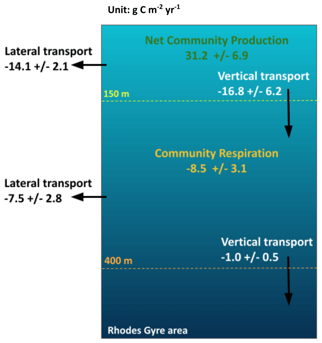
Figure 9 Annual organic carbon budget ($\mathrm{g}\mathrm{C}{\mathrm{m}}^{-\mathrm{2}}{\mathrm{yr}}^{-\mathrm{1}}$) in the surface and intermediate layers of the Rhodes Gyre for the 7-year period 2013–2020.

The biogeochemical fluxes, i.e., PP, CR, and NCP, all show an annual mean stronger than the 7-year average during the cold winter years of 2016–2017, 2018–2019, and 2019–2020 (Table 1). However, the magnitude of PP and CR appears to be higher for the mild winter year of 2017–2018 compared to the cold winter year of 2014–2015. Regarding the physical transfer, we found that particulate and dissolved OC downward export show a clearly stronger annual mean during all cold winter years (2014–2015, 2016–2017, 2018–2019, and 2019–2020). The lateral export in the surface is generally also stronger during cold years, except during the year 2016–2017, which shows the lowest lateral OC export. Nevertheless, this latter year shows both the highest OC downward export from the surface and the highest lateral export in the intermediate layer towards the surrounding region, suggesting that lateral export is deepened during this very cold winter (Fig. 5c). Finally, the excess of biological production during cold winters is almost entirely compensated by an excess in total OC export.

4 Discussion

4.1 Model skill assessment

The comparisons of model results with the available data sets, presented in Sect. 3.1, show an overall good agreement in the seasonal dynamics and vertical distribution of chlorophyll, nutrients, and dissolved oxygen in the Levantine Sea. We notice, however, an underestimation in the magnitude of the modeled subsurface maximum of chlorophyll and dissolved oxygen concentration when comparing with both the BGC-Argo float and cruise data. The model also produces chlorophyll maxima that are too deep in summer and profiles that are too mixed in winter. Concerning the overestimation of the maximum depths, further studies will be necessary to improve the model parameterizations (optical model, POC degradation processes, particle sinking). Concerning the too-strong homogenization of the winter profiles, we notice that in winter, mixed chlorophyll and DCM-like profiles alternate, indicating small-scale (few kilometers) or temporal variability related to meteorological conditions. The study of the physical processes driving this variability and their impact on phytoplankton deserves a dedicated study of physical and biogeochemical Argo profiles and probably a higher spatial resolution modeling.

One should notice that ocean color and in situ data remain scarce in the Levantine Sea and especially in the Rhodes Gyre (D'Ortenzio et al., 2021), making the evaluation exercise difficult and partial. Additional in situ observations in the study area are required to further refine the biogeochemical model results. Comparisons with complementary biological (in particular composition and biomass of phytoplankton and zooplankton) and biogeochemical observations carried out during the PERLE cruises, whose analyses are in progress, will be used in near-future studies to continue the evaluation.

Here, we complete the direct comparisons with in situ and satellite observation comparisons from the literature. In the model results, DOC concentrations show a rapid decrease with depth from values ranging between 45 and 64 mmol C m⁻³ in the surface layer to values around 40 mmol C m⁻³ below 300 m depth (Fig. 6e). These results are in agreement with what was reported in previous observational studies in the Levantine Sea (Krom et al., 2005; Santinelli et al., 2010; Pujo-Pay et al., 2011; Martinez Perez et al., 2017). The surface values fall in the lower range of observations (41–100 mmol C m⁻³), which could be partly explained by the locations of the observations, mostly outside the Rhodes Gyre; indeed in the model results the concentrations are slightly lower in the Rhodes Gyre compared to the surrounding Levantine Sea. The model DOC concentrations exhibit a clear seasonal cycle in the surface layer, with maximum values at the end of summer and low values during winter mixing periods when surface waters are mixed with deeper DOC-poor waters and DOC is transported towards intermediate depths. This variability is in line with the few observational studies documenting the seasonal cycle in other regions of the Mediterranean, characterized by strong winter mixing such as the Ligurian and southern Adriatic seas (Avril, 2002; Santinelli et al., 2013).

Regarding the organic carbon biological fluxes, the 7-year averaged annual NPP that amounts to 115 ± 15 $\mathrm{g}\mathrm{C}{\mathrm{m}}^{-\mathrm{2}}{\mathrm{yr}}^{-\mathrm{1}}$ falls in the range of the previous annual estimates for the northern Levantine Sea based on satellite ocean color data (60–152 $\mathrm{g}\mathrm{C}{\mathrm{m}}^{-\mathrm{2}}{\mathrm{yr}}^{-\mathrm{1}}$; Antoine et al., 1995 ; Bosc et al., 2004; Uitz et al., 2012) or more specifically for the Rhodes Gyre based on modeling studies (92–180 $\mathrm{g}\mathrm{C}{\mathrm{m}}^{-\mathrm{2}}{\mathrm{yr}}^{-\mathrm{1}}$; Napolitano et al., 2000; Kalaroni et al., 2020; Cossarini et al., 2021). The higher magnitude of annual and winter NPP values in the Rhodes Gyre area compared to the surrounding Levantine Basin (Fig. S5d), by 13 % and 21 %, respectively, is in line with the findings of Vidussi et al. (2001), Uitz et al. (2012), and Cossarini et al. (2021).

The mean annual POC export at 150 m depth in the Rhodes Gyre is estimated in the model at 11.9 ± 3.4 $\mathrm{g}\mathrm{C}{\mathrm{m}}^{-\mathrm{2}}{\mathrm{yr}}^{-\mathrm{1}}$. The POC export data in the Mediterranean are almost all located in other regions (Gulf of Lion, Gogou et al., 2014; Adriatic Sea, Boldrin et al., 2002; Ionian Sea, Gogou et al., 2014) and show values measured or extrapolated at 100–150 m between 3 and 23 $\mathrm{g}\mathrm{C}{\mathrm{m}}^{-\mathrm{2}}{\mathrm{yr}}^{-\mathrm{1}}$. Only Moutin and Raimbault (2002) reported an estimate of POC export for the Rhodes Gyre but limited to May–June 1996. The value of 7.5 ± 0.9 $\mathrm{g}\mathrm{C}{\mathrm{m}}^{-\mathrm{2}}{\mathrm{yr}}^{-\mathrm{1}}$ is twice our mean value for the same months. It does not seem possible with these too-rare and punctual observations to conclude on a possible bias of the model.

The mean fraction of NPP exported from the surface under the particulate form represents 10 % of the total NPP in the model. This is in the range of what was estimated for the measured carbon export by Buesseler (1998) for the global ocean (2 %–20 %), similar to the estimates of 11 % for the western and eastern Mediterranean sites by Gogou et al. (2014) and to the estimates of 9 % by Moutin and Raimbault (2002) for the Rhodes Gyre.

Our estimate of the annual DOC export at 150 m depth amounts to 4.9 ± 2.8 $\mathrm{g}\mathrm{C}{\mathrm{m}}^{-\mathrm{2}}{\mathrm{yr}}^{-\mathrm{1}}$. It is smaller than the annual DOC flux estimated at 100 m at 12 $\mathrm{g}\mathrm{C}{\mathrm{m}}^{-\mathrm{2}}{\mathrm{yr}}^{-\mathrm{1}}$ in the Ligurian Sea by Avril (2002) and at 50 m depth at 15.4 $\mathrm{g}\mathrm{C}{\mathrm{m}}^{-\mathrm{2}}{\mathrm{yr}}^{-\mathrm{1}}$ in the southern Adriatic Sea by Santinelli et al. (2013), both sites being characterized by strong winter mixing. On the contrary, our estimate is greater than the DOC flux at 50 m of 3.2 $\mathrm{g}\mathrm{C}{\mathrm{m}}^{-\mathrm{2}}{\mathrm{yr}}^{-\mathrm{1}}$, estimated in the stratified Tyrrhenian Sea by Santinelli et al. (2013).

The modeled organic carbon fluxes appear to be in the order of magnitude of those deduced from observations, although we are conscious that the comparisons between both estimates are not straightforward, due notably to the definition of the processes (Ducklow and Doney, 2013; Di Biagio et al., 2022), the composition of OC considered (Gali et al., 2022), and the difference in time and locations.

Finally, though the model results show positive and negative annual variations of organic carbon inventory, an increasing trend in the OC inventory of 0.44 $\mathrm{mol}\mathrm{C}{\mathrm{m}}^{-\mathrm{2}}{\mathrm{yr}}^{-\mathrm{1}}$ is found over the period of 2013–2020. This is in general agreement with the observations by Ozer et al. (2022). In their study, these authors found a general long positive trend, superimposed by interannual variations, for the depth-integrated chlorophyll measured offshore of Haifa, to the east of the Levantine Basin, between 2002 and 2021. They suggested that the long-term warming and salinification result in an increased buoyancy and a shallowing of the LIW (up to 110 m), enabling a higher level of nutrients to become available to the photic zone from below, supporting the observed rise of the integrated chlorophyll a. Considering the lack of data in the study area to assess this point in the model and the high interannual variability, an extension of the simulation over a longer period would be needed to detect a possible drift in the model.

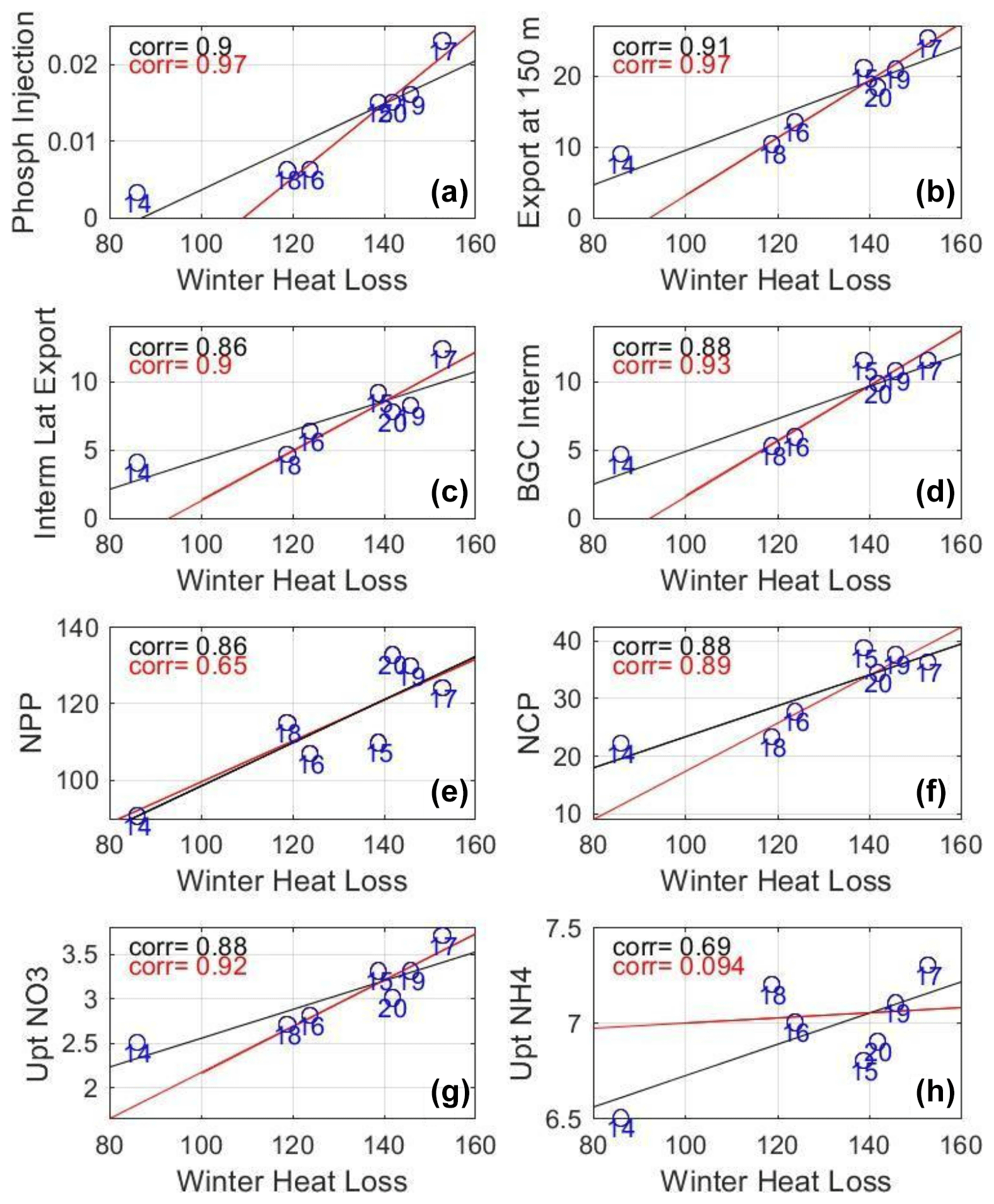
Figure 10 Scatter plot of winter surface heat loss (W m⁻²) vs. (a) winter phosphate injection (mol P m⁻²) into the surface layer and mean annual values of (b) downward export of OC (organic carbon) at 150 m ($\mathrm{g}\mathrm{C}{\mathrm{m}}^{-\mathrm{2}}{\mathrm{yr}}^{-\mathrm{1}}$), (c) lateral export from the intermediate layer ($\mathrm{g}\mathrm{C}{\mathrm{m}}^{-\mathrm{2}}{\mathrm{yr}}^{-\mathrm{1}}$), (d) biogeochemical consumption in the intermediate layer ($\mathrm{g}\mathrm{C}{\mathrm{m}}^{-\mathrm{2}}{\mathrm{yr}}^{-\mathrm{1}}$), (e) NPP, (f) NCP ($\mathrm{g}\mathrm{C}{\mathrm{m}}^{-\mathrm{2}}{\mathrm{yr}}^{-\mathrm{1}}$), and (g, h) uptake of nitrate and ammonium ($\mathrm{mmol}\mathrm{N}{\mathrm{m}}^{-\mathrm{2}}{\mathrm{yr}}^{-\mathrm{1}}$). The years are identified by the numbers in blue, e.g., 14 stands for 2013–2014. The black line shows the 7-year linear regression, and the red line shows the linear regression when excluding 2013–2014. The corresponding correlations are shown with the same color code.

4.2 Influence of winter mixing on phytoplankton growth

The model results display a similar general seasonal cycle of phytoplankton net growth from the years 2013–2014 to 2019–2020 in the Rhodes Gyre area. On average, the period of phytoplankton accumulation at the surface is concomitant with the global period of vertical mixing. This is in agreement with the modeling results for the whole Levantine Sea by Lazzari et al. (2012) and the satellite and BGC-Argo observations in the Rhodes Gyre reported by Lavigne et al. (2013), Mignot et al. (2014), and D'Ortenzio et al. (2021). Although this similar general pattern of ecosystem dynamics can be found for all the studied years, the model results exhibit pronounced interannual variability over the period in terms of magnitude and timing of nutrient injection into the surface and phytoplankton growth. Our model results show that during cold winters (years 2014–2015, 2016–2017, 2018–2019, and 2019–2020), deeper mixing leads to higher nutrient supply into the euphotic layer, with nutrient injection being more than twice as high during severe winters compared to mild winters. The significant correlation found between nutrient injection and mean winter HL (heat loss, Fig. 10a) or mean winter MLD (higher than 0.85) is in line with previous observational (Ediger and Yilmaz, 1996; Yilmaz and Tugrul, 1998) and modeling (Napolitano et al., 2000) studies in the Rhodes Gyre.

The model shows that, during cold winters, phytoplankton growth is interrupted during strong mixing periods and is explosive at the end of strong mixing periods. This is in line with the study of Ediger et al. (2005), who reported higher PP and biomass at the periphery of the gyre than in its homogenized center, based on observations collected in March 1992 when a deep convection event occurred. However, we show that in the Rhodes Gyre the episodes of strong surface phytoplankton growth, as well as of its interruption due to vertical mixing deeper than the base of the euphotic zone, remain short. They are markedly shorter than in the other Mediterranean regions of deep water formation, especially compared to the northwestern Mediterranean region, where deep mixing can last for 2 months during intense convection years (i.e., 2004–2005, 2005–2006, 2012–2013; Bernardello et al., 2012; Ulses et al., 2016; Mayot et al., 2017; Kessouri et al., 2018). These results are consistent with the characterization proposed by D'Ortenzio and Ribera d'Alcala et al. (2009) and Mayot et al. (2016) as an intermittent or intermediate bloom regime.

Although winter and spring NPP is higher under cold winters, annual NPP is not significantly correlated with winter heat loss if 2013–2014, the warmest winter year, is not considered (Fig. 10e). The modeled NPP depends on the nitrate and ammonium uptake supporting, respectively, 30 % and 70 % of it. Nitrate uptake is significantly correlated with winter HL (R =  0.88, p value < 0.01, Fig. 10g) and MLD, whereas the ammonium uptake shows no significant correlation with winter HL (R =  0.69, p value < 0.01, Fig. 10h). Thus the intensity of mixing that determines the amount of new deep nutrients available for primary production does not strongly impact recycled production. Other driving factors such as trends in temperature and nutricline depth as observed in the southeastern Levantine Basin (Ozer et al., 2022) or low solar insolation in summer/fall that we do not address in this study could also influence the variability of annual PP.

4.3 Influence of winter mixing on carbon export and sequestration

At the annual scale, the planktonic ecosystem in the Rhodes Gyre acts as a sink of atmospheric CO₂ with an estimate of mean NCP at 31.2 ± 6.9 $\mathrm{g}\mathrm{C}{\mathrm{m}}^{-\mathrm{2}}{\mathrm{yr}}^{-\mathrm{1}}$. This OC net biological production (dissolved inorganic carbon, DIC, consumption) is almost balanced by both the OC lateral and vertical transports with a quasi-even distribution. The high interannual variability of annual NCP (SD of 22 %) in the Rhodes Gyre appears to be primarily linked to the intensity of winter atmospheric HL and vertical mixing (significant correlation > 0.88 between annual NCP and winter HL, Fig. 10f), which indicates an enhanced autotrophic metabolism during cold years that is almost counterbalanced by an enhanced OC export. The OC exported towards the intermediate layer is further respired or laterally exported towards the surrounding Levantine Basin. Finally, we estimate that 1 % and 3 % of the NPP and NCP, respectively, is then transferred towards the deeper depths.

Figure 10b and c shows the relationship between winter heat loss and annual vertical export of organic carbon at 150 m and the lateral flux of organic carbon from the intermediate layer (150–400 m) exported from the Rhodes Gyre to the Levantine Basin. The correlation for those annual exports is greater than 0.86 (p value < 0.02) for the 7-year data set and increases to more than 0.90 (p value < 0.005) if 2013–2014, the warmest winter year, is removed. Compared to the linear regression inferred from the other 6 years (red line), 2013–2014 is above the regression line, meaning stronger vertical and horizontal fluxes than predicted by the regression (values approaching 0 or even negative). Unlike the other years, the seasonal cycle of export at 150 m indeed shows no clear signal in winter (Fig. 7e). It is likely that the fluxes of the year 2013–2014, which are weaker but close to those of the second warmest year (2017–2018), can be considered minimum values for the Rhodes Gyre. Compared to these minimum values, the annual exports are increased by a factor of 2 to 2.5 for the coldest years of the sequence, with these increases thus representing the contribution of cold winters.

The order of magnitude of the winter contribution to the annual vertical export is similar to that found by Kessouri et al. (2018) at the same depth in the deep convection zone of the Gulf of Lion in the northwestern Mediterranean. The main difference is on the timing of the vertical export. Bernardello et al. (2012) and Kessouri et al. (2018) showed that in the Gulf of Lion, the production and export phases alternate, the former mainly between gales when the layer is stratified and the latter during gales and deep vertical mixing. In the Rhodes Gyre where convection is intermediate, the depth of mixing is not sufficient to persistently inhibit production, which allows for more continuous export throughout the winter period. Intermittency of convection is thus less necessary to trigger the export than for deep convection. This could explain the compensation between the excess in NCP and OC export during cold winters.

The clear relation between winter severity and both annual OC vertical export at 150 m and lateral OC flux from the Rhodes Gyre to the Levantine Basin in the intermediate layer allows us to identify the responsibility of physical processes of LIW formation followed by subduction from the Rhodes Gyre to the Levantine Basin. Taillandier et al. (2022) indicated that the volume of dense water in the Rhodes Gyre region returns to its pre-convection level in 2 to 3 months, which gives an estimate of the timescale of lateral export that is in agreement with the model's assessment showing lateral export of organic carbon from the intermediate layer of the Rhodes Gyre that becomes low from April onwards (Fig. 8b). Regarding organic carbon, these physical processes (convection/subduction) are modulated by biogeochemical processes, for example, consumption by respiration which competes with physical export.

In this study, we describe only partially the cycle of DIC through its biological consumption. Air–sea flux and transport terms of the inorganic form of carbon are not considered here. This limits the determination of the role of the Rhodes Gyre relative to atmospheric CO₂ uptake and of the influence of winter mixing intensity on this uptake. Previous studies reported that a significant amount of OC exported below the euphotic layer could be reinjected back under organic or remineralized form during the following winters in convection regions (Oschlies, 2004; Körtzinger et al., 2008; Palevsky and Quay, 2017). Over the study period, one can notice the succession of 2 convective years, 2018–2019 and 2019–2020; however, the second year does not display particularly low net OC downward export compared to the other cold years (Fig. 10b). The impact of winter mixing on total carbon sequestration is thus difficult to establish and requires the description of the dynamics of the carbonate system in the model that will be investigated in a near-future study.

Based on a 1D coupled model combined with satellite data, D'Ortenzio et al. (2008) and Taillandier et al. (2012) reported a CO₂ air–sea flux between −1.5 and −0.5 $\mathrm{mol}\mathrm{C}{\mathrm{m}}^{-\mathrm{2}}{\mathrm{yr}}^{-\mathrm{1}}$ in the Rhodes Gyre and the whole Levantine Sea, acting thus as a source for the atmosphere. Cossarini et al. (2021) modeled the temporal evolution of CO₂ air–sea fluxes from 1999 to 2019. They found that the Rhodes Gyre is a small sink of atmospheric CO₂ (< 0.25 $\mathrm{mol}\mathrm{C}{\mathrm{m}}^{-\mathrm{2}}{\mathrm{yr}}^{-\mathrm{1}}$), whereas the surrounding Levantine Basin is a source for the atmosphere. Besides, they reported an increasing absorption of atmospheric CO₂ in both the eastern and western Mediterranean Sea, leading to a change in the sign of air–sea exchanges averaged over the eastern Mediterranean, and a switch from source to sink at the end of the period (2019), in response to the increase of atmospheric CO₂. Hassoun et al. (2019) and Wimart-Rousseau et al. (2021) derived an increasing trend in inorganic carbon content in the coastal and open-sea Levantine Basin, based on observations. The predictions for the carbon cycle in the Mediterranean Sea over the 21st century by Solidoro et al. (2022) and Reale et al. (2022) showed a further increase in atmospheric CO₂ absorption, which, together with the increasing temperature and stratification (Somot et al., 2006; Soto-Navarro et al., 2020), leads to an increase in carbon content.

5 Conclusion

In this study we have used a 3D coupled hydrodynamic–biogeochemical model to investigate the pelagic ecosystem functioning and estimate a budget of organic carbon in the Rhodes Gyre, over the period of 2013–2020, marked by the alternation of cold and mild winter years. The assessment of the model results based on satellite, cruise, and BGC-Argo float observations in the Levantine Basin demonstrates that the model was able to reproduce the main seasonal and spatial evolution of physical and biogeochemical observed variables reasonably well.

The model confirms that the intensity of winter surface heat loss and vertical mixing events significantly influences the magnitude of nutrient supplies into the euphotic layer and of surface phytoplankton growth. The development of phytoplankton at the surface is always concomitant with the winter mixing period. It is characterized by a first phase of progressive growth with the deepening of the mixed layer and a second phase consisting of alternating short periods (< 2 weeks) of vertical mixing and of phytoplankton growth episodes during temporary restratification. This second phase only occurs during severe winters due to the dilution of phytoplankton biomass over the mixed layer and the reduction of light availability. A spatial variability is also depicted in the gyre during the mixing period. Under prolonged winter conditions, the characteristics of the phytoplankton bloom are present at the periphery of the Rhodes Gyre, when vertical mixing is intense, and reappear in the center of the gyre at the restratification. At the end of the mixing period, a DCM forms and progressively deepens until mid-summer.

OC is transported vertically towards intermediate depths and laterally towards the surrounding regions, partly by subduction during the dispersion of LIW. The annual downward OC export is strongly enhanced with the intensity of winter surface heat flux, with annual export being 2 to 2.5 times higher during cold winter years compared to mild winter years. In the Rhodes Gyre, 50 % of the organic carbon exported below 150 m depth is remineralized at intermediate levels inside the gyre, and 45 % is exported towards the surrounding Levantine Basin. The Rhodes Gyre acts as a source of organic carbon for the surrounding areas.

The Rhodes Gyre is found to be an autotrophic ecosystem, with net community production in the surface layer accounting for 31.2 ± 6.9 $\mathrm{g}{\mathrm{m}}^{-\mathrm{2}}{\mathrm{yr}}^{-\mathrm{1}}$. Finally, our modeling study is constrained to the Rhodes Gyre and a 7-year period. Its spatial and temporal extension could allow the examination of (i) the fate of the organic carbon produced in the Rhodes Gyre after its export to the Levantine Basin and to the other regions of the eastern Mediterranean Sea and (ii) the influence of remote drivers on biological activity and physical processes in the Levantine Basin.