Gross primary productivity and the predictability of CO₂: more uncertainty in what we predict than how well we predict it

The prediction of atmospheric CO₂ concentrations is limited by the high interannual variability (IAV) in terrestrial gross primary productivity (GPP). However, there are large uncertainties in the drivers of GPP IAV among Earth system models (ESMs). Here, we evaluate the impact of these uncertainties on the predictability of atmospheric CO₂ in six ESMs. We use regression analysis to determine the role of environmental drivers in (i) the patterns of GPP IAV and (ii) the predictability of GPP. There are large uncertainties in the spatial distribution of GPP IAV. Although all ESMs agree on the high IAV in the tropics, several ESMs have unique hotspots of GPP IAV. The main driver of GPP IAV is temperature in the ESMs using the Community Land Model, whereas it is soil moisture in the ESM developed by the Institute Pierre Simon Laplace (IPSL-CM6A-LR) and in the low-resolution configuration of the Max Planck Earth System Model (MPI-ESM-LR), revealing underlying differences in the source of GPP IAV among ESMs. Between 13 % and 24 % of the GPP IAV is predictable 1 year ahead, with four out of six ESMs showing values of between 19 % and 24 %. Up to 32 % of the GPP IAV induced by soil moisture is predictable, whereas only 7 % to 13 % of the GPP IAV induced by radiation is predictable. The results show that, while ESMs are fairly similar in their ability to predict their own carbon flux variability, these predicted contributions to the atmospheric CO₂ variability originate from different regions and are caused by different drivers. A higher coherence in atmospheric CO₂ predictability could be achieved by reducing uncertainties in the GPP sensitivity to soil moisture and by accurate observational products for GPP IAV.

1 Introduction

Near-term predictions of atmospheric CO₂ concentrations are an essential step towards the evaluation of climate mitigation efforts and the development of carbon monitoring programmes (Ilyina et al., 2021). However, the high interannual variability (IAV) in land–atmosphere carbon fluxes, specifically gross primary productivity (GPP), drives the variability in atmospheric CO₂ and limits its predictability (Piao et al., 2020). Therefore, the skilful prediction of GPP is a crucial step towards the real-time verification of anthropogenic carbon emissions and the evaluation of mitigation efforts.

The usual approach to evaluate the predictability of an Earth system variable is to compare predictions to observed values. In the case of GPP, this is complicated by the uncertainty in GPP observations (Zhang and Ye, 2021). As an alternative to calculating the actual predictability that is based on observations, the potential predictability can be assessed by evaluating how well the models can predict their own carbon flux variability. To do this, an ensemble of simulations with an Earth system model (ESM) is initialized from quasi-identical conditions. In a system with little predictability, the spread among the ensemble members increases quickly until all predictive capability is lost when the ensemble spread reaches the magnitude of the IAV. There are, however, certain processes in the Earth system that provide predictability and hinder the divergence of the ensemble members. For example, the El Niño–Southern Oscillation (ENSO) produces predictable climate anomalies that have a sustained impact on GPP (Zeng et al., 2008; Betts et al., 2016). Other processes extend predictability by providing “memory” that maintains the initial conditions. Soils, for example, store initial moisture anomalies by acting as a buffer between the atmosphere and the vegetation (Bellucci et al., 2015). Soil moisture anomalies are further extended through land–atmosphere coupling, which creates a feedback loop that enhances the persistence of these anomalies (Kumar et al., 2020). The initial conditions of the simulations are maintained through the lagged response of plant growth to climatic conditions. Slowly reacting vegetation can cause precipitation anomalies or prolonged drought (Alessandri and Navarra, 2008; Zhang et al., 2021). Given all of these mechanisms of predictability, we find that terrestrial carbon fluxes are predictable for 2 years (Ilyina et al., 2021).

Although several ESMs reproduce the same predictability horizon for globally integrated terrestrial carbon fluxes (Séférian et al., 2018; Ilyina et al., 2021; Spring and Ilyina, 2020; Lovenduski et al., 2019), there are substantial differences in the spatial patterns of GPP IAV (Anav et al., 2015; O'Sullivan et al., 2020). The reason for these differences lies in poorly constrained ecosystem processes that have a large impact on GPP. One of these differences arises from the uncertainty in the sensitivity of GPP to environmental drivers (Ahlström et al., 2015; Jung et al., 2017; Beer et al., 2010; Piao et al., 2020; Collalti et al., 2020). The sensitivity of GPP to temperature and precipitation varies among studies, leading to ongoing discussion concerning the dominant driver of global carbon fluxes (Piao et al., 2020). The different sensitivity of GPP to precipitation across ESMs is further exacerbated by the large disagreement in water storage anomalies (Wu et al., 2021). The simulated annual cycle of water storage anomalies of major river basins is between 0.1 and 2 times that of the observed variability. These deviations in hydrological variability between models are likely to cause similar deviations in GPP IAV, especially in semi-arid watersheds. Further differences in GPP IAV are due to variations in ecosystem boundaries and the related spatial distribution of plant productivity. The Amazon rainforest, for instance, is a hotspot of land–atmosphere carbon fluxes and provides a large contribution to the predictability of atmospheric CO₂ (Zeng et al., 2008; Séférian et al., 2018; Ilyina et al., 2021). However, the transition zone between the wet tropical forest and semi-arid tropics within the Amazon Basin varies among the models due to differences in their representation of land cover (Collier et al., 2018; Hu et al., 2022). Such differences in biome boundaries also modify the impact of ENSO on GPP IAV. ENSO produces distinct spatial patterns of climatic anomalies that significantly influence the GPP on 32 % of the vegetated land area (Zhang et al., 2019). These ENSO-related climate patterns will have a different impact on GPP depending on the type of biomes under their influence. In addition to the spatial variability, many ESMs struggle to reproduce the seasonal variability in carbon fluxes. This can be seen in the large biases in phenology (Song et al., 2021). Several models overestimate the seasonal amplitude of leaf area index (LAI) in the tropics and mismatch the timing of the LAI maxima and minima (Peano et al., 2019, 2021).

All of these uncertainties suggest that there are large differences in the patterns of GPP IAV among the ESMs, but it is currently unclear how these differences affect the predictability of GPP. With this study, we want to extend our understanding of GPP predictability by considering the different patterns of GPP IAV among the ESMs. In a multi-model analysis, we investigate which processes drive the IAV in GPP and which processes allow the GPP IAV to be predictable. Regression analysis is used to determine the role of three environmental variables (soil moisture, temperature, and radiation) on GPP IAV and GPP predictability. We analyse the cause of differences in GPP predictability across ESMs, identify the areas of large discrepancies, and determine the factors contributing to the attached uncertainties. The aim of this study is to reveal which factors of GPP representation are limiting the predictability of atmospheric CO₂.

2 Methods

2.1 Data sources

We analyse model output from the Decadal Climate Prediction Project (DCPP; Boer et al., 2016). This protocol-driven multi-model approach aims at studying the decadal predictability of the Earth system with hindcasts, quasi-real-time forecasts, and case studies on predictability mechanisms. The hindcasts are initialized annually from 1960 to 2017 or 2019 with the starting dates between November and January and at least 10 ensemble members. Simulations are driven by Coupled Model Intercomparison Project Phase 5 (CMIP5) or Phase 6 (CMIP6) historical forcing and extended by Representative Concentration Pathway (RCP) 4.5 or Shared Socioeconomic Pathway (SSP) 2-4.5 afterwards. The DCPP framework does not prescribe any specific initialization or data assimilation methods and leaves these details to be decided by the respective modelling centres.

We additionally use the Community Earth System Model 2 (CESM2) output from the Seasonal-to-Multiyear Large Ensemble (SMYLE) prediction system (Yeager et al., 2022). The SMYLE hindcasts ensembles are initialized four times per year with 20 ensemble members between 1970 and 2019. In this study, the November initializations are used to achieve the highest comparability with the DCPP hindcasts.

We compare the spatial GPP IAV patterns of the ESMs with observation-based GPP products. Because of the uncertainty among observations, we include products based on three different sources. The Vegetation Photosynthesis Model (VPM; Zhang et al., 2017) is a remote-sensing-based product that uses a light use efficiency (LUE) model to calculate GPP. VPM uses satellite data from MODIS and an improved LUE algorithm that considers leaf quality. The second data set is GOSIF (Li and Xiao, 2019) which is based on data from MODIS and the Orbiting Carbon Observatory-2. GOSIF uses solar-induced chlorophyll fluorescence, which is a more recent approach, to calculate GPP. Lastly, we use FLUXCOM (version RS–METEO, ERA5; Jung et al., 2019), which uses machine learning to upscale flux tower observations with meteorological and remote-sensing data. Because FLUXCOM underestimates the IAV in GPP (Anav et al., 2015; O'Sullivan et al., 2020), it is recommended to scale the data so that the IAV of integrated FLUXCOM fluxes resembles observations (Jung et al., 2019). The VPM, GOSIF, and FLUXCOM data are linearly detrended before calculating the IAV. Due to its long time span, FLUXCOM is detrended over two periods (1979–1999 and 2000–2018).

CanESM5

The Canadian Earth System Model version 5 (CanESM5; Swart et al., 2019) consists of the Canadian Land Surface Scheme (CLASS) and Canadian Terrestrial Ecosystem Model (CTEM) with a T63 grid with an approximate resolution of 2.8^∘. The atmosphere is realized with the Canadian Atmospheric Model (CanAM5) with 49 vertical levels. Ocean physics is simulated with CanNEMO, on a tripolar grid with a resolution of 1 to $\mathrm{1}/\mathrm{3}$^∘ and 45 vertical levels, and ocean biogeochemistry is represented by the Canadian Model of Ocean Carbon (CMOC).

The CanESM5 hindcast simulations are initialized every January between 1960 and 2017 with 20 members. The 3D potential temperature and salinity of the global oceans are nudged toward the monthly Ocean Reanalysis System 5 (ORAS5; Zuo et al., 2019). Sea surface temperatures are nudged to the Extended Reconstructed Sea Surface Temperature (ERSSTv3; Xue et al., 2003; Smith et al., 2008) until 1981 and to the Optimum Interpolation Sea Surface Temperature (OISST; Banzon et al., 2016) afterwards. Sea ice concentration is nudged to the Hadley Centre Sea Ice and Sea Surface Temperature data set (HadISST.2; Titchner and Rayner, 2014), and sea ice thickness is nudged to monthly climatology until 1988 and to the SMv3 statistical model of Dirkson et al. (2017) afterwards. For the atmosphere, temperature, horizontal wind components, and specific humidity are nudged to ERA-40 (Uppala et al., 2005) until 1978 and to 6-hourly ERA-Interim data (Dee et al., 2011) afterwards.

CESM1-CAM5

The Community Earth System Model (CESM) version 1.1 (Hurrell et al., 2013) is used to produce 40-member simulations in the Decadal Prediction Large Ensemble (DPLE) project (Yeager et al., 2018). The model components are the Community Land Model version 4 (CLM4; Lawrence et al., 2011) with a 1^∘ resolution, the Community Atmosphere Model version 5 (CAM5) with 30 vertical levels, the Parallel Ocean Program (POP2) with 60 vertical levels, and sea ice with the Community Ice Code (CICE4).

The CESM1-CAM5 hindcasts are initialized every November. There is no direct assimilation of observations to produce the initial conditions; instead, ocean and sea ice are obtained from simulation runs forced by historic atmospheric surface fields (Yeager et al., 2018). Initial conditions for the land and atmosphere components are obtained from ensemble member no.34 of the CESM Large Ensemble (Kay et al., 2015; Lovenduski et al., 2019).

CESM2

CESM version 2 (Danabasoglu et al., 2020) runs on a 1^∘ horizontal resolution for all components. The atmosphere is simulated by the Community Atmosphere Model version 6 (CAM6) with 32 vertical levels. The ocean model is the Parallel Ocean Program version 2 (POP2) with 60 vertical levels, with the biogeochemistry from the Marine Biogeochemistry Library and sea ice by CICE version 5.1.2 (CICE5) with 8 vertical layers. The land component is simulated by the Community Land Model version 5 (CLM5; Lawrence et al., 2019), which has several updates to its predecessors CLM4 and CLM4.5, leading to a better representation of the global carbon cycle in benchmarks (Bonan et al., 2019).

Hindcasts are initialized on the first day of every November, February, May, and August, and they run for 24 months. Only the November initializations are used in this analysis to increase comparability with the DCPP simulations. Initial conditions for the atmosphere, ocean, and sea ice stem from the Japanese 55-year Reanalysis – JRA-55 (Kobayashi et al., 2015) and JRA55-do (Tsujino et al., 2018). The land surface and biogeochemistry are initialized from forced CLM5 simulations.

CMCC-CM2-SR5

The Euro-Mediterranean Centre on Climate Change coupled climate model (CMCC-CM2; Cherchi et al., 2019; Lovato et al., 2022) is based on CESM and consists of the Community Land Model (CLM4.5) with a 1^∘ resolution and the atmospheric model CAM5.3 with 30 vertical levels. The distinguishing element of CMCC-CM is the ocean, which is simulated by NEMO3.6, while sea ice is modelled by CICE4.

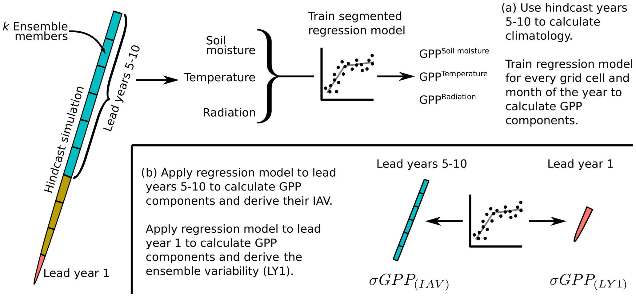
Figure 1 Workflow of the statistical analysis. In panel (a), lead years 5 to 10 of the hindcast simulations are used to train a regression model that calculates the components of GPP caused by the environmental drivers. In panel (b), the regression model is applied to lead years 5 to 10 to calculate the IAV in the GPP components (σGPP_(IAV)) and to lead year 1 to calculate the mean ensemble spread of the GPP components (σGPP_(LY1)).

The 10-member hindcast simulations are initialized every November (Nicolì et al., 2023). The ocean initial conditions are from CHOR (Yang et al., 2017) until 2010 and from CGLORSv7 (Storto and Masina, 2016) afterwards. The atmosphere is initialized from ERA-40 until 1978 and from ERA-Interim afterwards. The land surface is initialized using the reanalysis with two different meteorological forcings. For this reason, only ensemble members 1, 3, 5, 7, 8, and 9 are used, as the other members start from a different state and this would not allow for the quantification of predictability by ensemble spread.

Because the CMCC-CM2-SR5 fields containing land–atmosphere carbon fluxes are not exported for the DCPP runs, the historical simulations are used to infer the relationship between environmental drivers and GPP.

IPSL-CM6A-LR

The ESM developed by the Institute Pierre Simon Laplace (IPSL; Boucher et al., 2020) uses the ORCHIDEE v2.0 (Cheruy et al., 2020) land surface model (LSM) with an average resolution of 157 km. The atmosphere is simulated at the same resolution by LMDZ6 with 79 vertical levels, the ocean is simulated with NEMO-OPA with a 1^∘ resolution and 75 vertical levels, and ocean biogeochemistry is simulated with PISCESv2.

The hindcast simulations of IPSL-CM6A-LR come from the DCPP project. The 10-member ensembles start annually in January between 1960 and 2016. The hindcasts are initiated from an assimilation run with EN4 sea surface temperatures (Good et al., 2013) and Atlantic sea surface salinity (Estella-Perez et al., 2020). Subsurface ocean, sea ice, and atmosphere are not assimilated.

MPI-ESM-LR

MPI-ESM-LR is the Max Planck Earth System Model (MPI-ESM1.1; Giorgetta et al., 2013) used in a low-resolution configuration. The land is simulated by JSBACH with dynamic vegetation (Reick et al., 2013). The ocean component is the Max Planck Institute for Meteorology Ocean Model (MPIOM) with a horizontal resolution of about 150 km and 40 vertical levels. The atmosphere is simulated by ECHAM at a T63 resolution with 47 vertical layers, and ocean biogeochemistry is represented by the Hamburg Ocean Carbon Cycle (HAMOCC) model.

The utilized hindcast simulations of MPI-ESM-LR are conducted within the MiKlip project (Marotzke et al., 2016). The decadal prediction system comprises 10-member ensembles starting every January between 1961 and 2014. Ocean temperature and salinity are initialized from the Ocean Reanalysis System 4 (ORAS4; Balmaseda et al., 2013), and the atmosphere is initialized from ERA-40 from 1960 to 1998 and from ERA-Interim from 1990 to 2014.

2.2 Statistical approach

Overview

An overview of the statistical analysis is shown in Fig. 1. Every hindcast simulation is initialized from quasi-identical conditions. With the increasing lead time, the variability within the hindcast ensemble (standard deviation across the ensemble members for a given time) also increases until it reaches the IAV. Based on this assumption, the hindcast simulations are split into two groups by lead time: lead year 1 and lead years 5 to 10. For lead years 5 to 10, the effects of ocean and atmosphere initialization are assumed to be negligible. These years are used to calculate the monthly mean climatology, which is removed from both groups to obtain the anomalies. The anomalies of lead years 5 to 10 are used in a regression analysis to derive the sensitivity of GPP to the environmental drivers, i.e. soil moisture, temperature, and radiation (Fig. 1a). The regression model is applied to the anomalies of lead years 5 to 10 to calculate the IAV in all GPP components (σGPP_(IAV)) and to the anomalies of lead year 1 to calculate the ensemble variability in all GPP components (σGPP_(LY1)) (Fig. 1b). We derive the predictability of GPP by comparing σGPP_(LY1) to σGPP_(IAV). Because the hindcast simulations are not evaluated against observations, the calculated predictability reflects the potential predictability.

Climatology and sensitivity

The monthly mean climatologies are calculated from lead years 5 to 10, with a 3-year moving-window approach for every calendar year. Because the moving-window method is not applicable for the first decade of hindcast initializations, the monthly climatology for the 1960s (1970s for CESM2) is calculated based on all lead years 5 to 10 within the 1960s (or 1970s). Anomalies of all input fields are calculated by subtracting the monthly climatologies from the hindcast data. The obtained anomalies of lead years 5 to 10 make up a data set of n simulation years:

$$\begin{array}{}\text{(1)}& \begin{array}{rl}n=& \text{6 hindcast years }\times \text{no. ensemble members }\\ & \times \text{no. initializations}.\end{array}\end{array}$$

A total of 10 to 40 ensemble members and 56 to 58 initializations result in sample sizes of 3330 to 13 680. Because the hindcast length is only 2 years for the CESM2 simulations, a different approach is used here. Instead of lead years 5 to 10, only lead year 2 is selected and only five random ensemble members are used from every hindcast to reduce the number of simulations with the same initial conditions. To offset the reduced number of data points, five random simulations are also added from the hindcast simulations initialized in February, May, and August.

The resulting data set of lead year 5 to 10 anomalies is used to derive the sensitivity of GPP to the environmental drivers (ENV: soil moisture, temperature, and radiation) by fitting a regression model for every grid cell and month of the year. The relationship between GPP and the environmental drivers is frequently non-linear, sometimes due to specific breakpoints in the functional representation of GPP. For this reason, segmented linear regression (SLR) is used to model GPP from the environmental drivers (Muggeo, 2008). SLR finds breakpoints in the data, splitting them into multiple ranges and fitting an individual regression model to each of the data ranges. Here, a single breakpoint is determined for each of the three predictor variables.

Because environmental drivers have some degree of collinearity, the regression analysis will not be able to fully attribute the GPP anomalies to their specific causes. Therefore, the resulting sensitivities should be taken as a “contributive” and not a “true” effect of the environmental drivers (Wang et al., 2016).

Variability and predictability

The SLR can now be applied to individual simulations to determine the component of GPP anomalies that can be attributed to each of the environmental drivers:

$$\begin{array}{}\text{(2)}& \begin{array}{rl}\mathrm{\Delta }\mathrm{GPP}\approx & \mathrm{\Delta }{\mathrm{GPP}}^{\mathrm{Soil}\mathrm{moisture}}+\mathrm{\Delta }{\mathrm{GPP}}^{\mathrm{Temerature}}\\ & +\mathrm{\Delta }{\mathrm{GPP}}^{\mathrm{Radiation}}.\end{array}\end{array}$$

The three components of GPP anomalies (ΔGPP^ENV) are calculated for every simulation within the hindcast lead time 5 to 10. From the results, we calculate the IAV in the components for every grid cell and month of the year ($\mathit{\sigma }{\mathrm{GPP}}_{\left(\mathrm{IAV}\right)}^{\mathrm{ENV}}$). Similarly, the SLR is applied to the anomalies of lead year 1 to calculate the standard deviation for every month within the hindcast simulations. Averaging over the standard deviations of every hindcast returns the ensemble variability in lead year 1 ($\mathit{\sigma }{\mathrm{GPP}}_{\left(\mathrm{LY}\mathrm{1}\right)}^{\mathrm{ENV}}$).

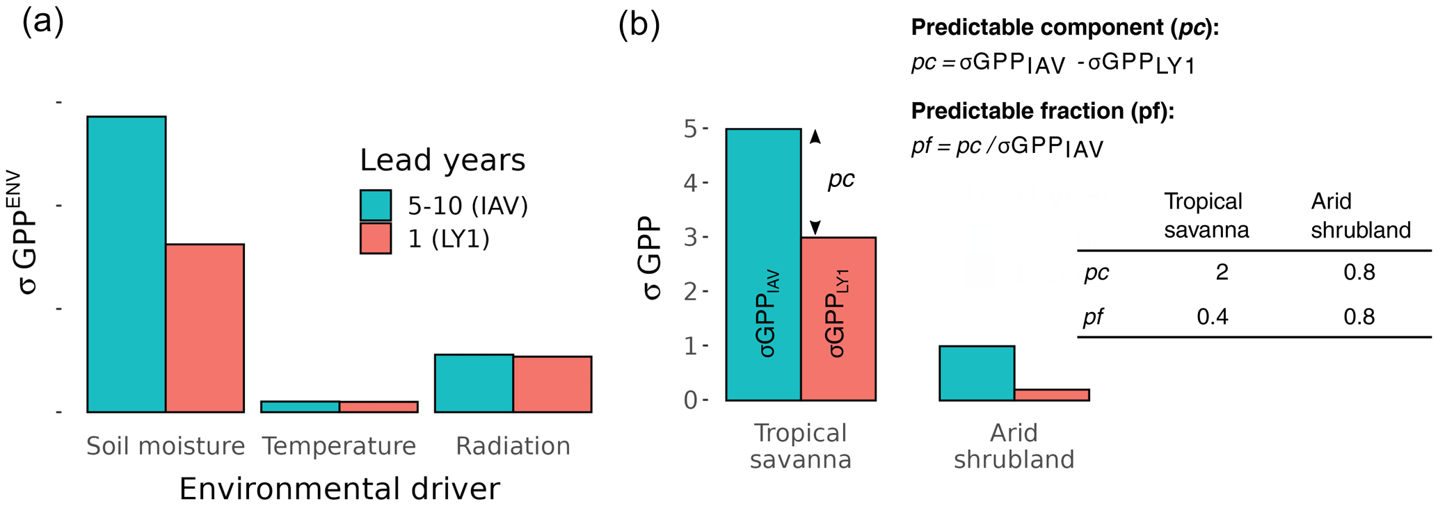
Figure 2 Panel (a) presents the exemplary composition of GPP variability and predictability in a tropical forest. The components of GPP IAV are calculated from lead years 5 to 10 (green bars) and the ensemble variability is calculated from lead year 1 (red bars). In the exemplified region, most of the variability is caused by soil moisture and radiation, and GPP is not restricted by temperature. Predictability is exclusively provided through soil moisture. Panel (b) demonstrates the need for the two predictability metrics using a tropical savanna and an arid shrubland as examples. The predictable component (pc) is the absolute predictable IAV, and the predictable fraction (pf) is the pc scaled by the IAV. While the arid shrubland has a better potential to retain memory (as seen from the high pf), these ecosystems contribute little to the variability in atmospheric CO₂, which can be better assessed using the pc.

The predictability is assessed by comparing σGPP_(LY1) to σGPP_(IAV). A high predictability of an input field means that the ensemble variability is restricted for some time after the hindcast initialization and does not reach the IAV immediately (Fig. 2a). In this study, we use two metrics to evaluate different aspects of predictability. We calculate the fraction of GPP IAV that is predictable (the predictable fraction – pf) to assess the ability of a system to retain memory. Although this metric is useful for quantifying the mechanisms that provide predictability at a local level, the pf is not suitable for assessing how GPP predictability affects the predictability of atmospheric CO₂. This is because the regions with a high pf do not necessarily contribute much to the global GPP fluxes. The regions with the highest pf values are often in deserts with very low carbon fluxes (Dunkl et al., 2021). To assess the contribution of GPP predictability to atmospheric CO₂ predictability, we calculate the absolute portion of the IAV that can be predicted as the predictable component (pc). The pc is the difference between IAV and ensemble variability and is generally higher in regions that contribute more to CO₂ IAV:

$$\begin{array}{}\text{(3)}& {\displaystyle }{\mathrm{pc}}^{\mathrm{ENV}}=\mathit{\sigma }{\mathrm{GPP}}_{\left(\mathrm{IAV}\right)}^{\mathrm{ENV}}-\mathit{\sigma }{\mathrm{GPP}}_{\left(\mathrm{LY}\mathrm{1}\right)}^{\mathrm{ENV}},\text{(4)}& {\displaystyle }{\mathrm{pf}}^{\mathrm{ENV}}={\displaystyle \frac{{\mathrm{pc}}^{\mathrm{ENV}}}{\mathit{\sigma }{\mathrm{GPP}}_{\left(\mathrm{IAV}\right)}^{\mathrm{ENV}}}}.\end{array}$$

The use of the two predictability metrics is exemplified in Fig. 2b.

3 Results and discussion

3.1 Patterns of GPP IAV

In order to understand what the models are predicting, we start by analysing the patterns of GPP IAV. There are differences in the overall magnitude of GPP IAV among ESMs, with CanESM5, CMCC-CM2-SR5, and IPSL-CM6A-LR at the lower end of the IAV spectrum, whereas CESM2 and MPI-ESM-LR are at the higher end of the IAV spectrum. Factors that could explain some of the differences in the overall magnitude of IAV are the relatively weak ENSO teleconnection in CanESM5 (Swart et al., 2019) or the low total GPP in CMCC-CM2-SR5 (Lovato et al., 2022).

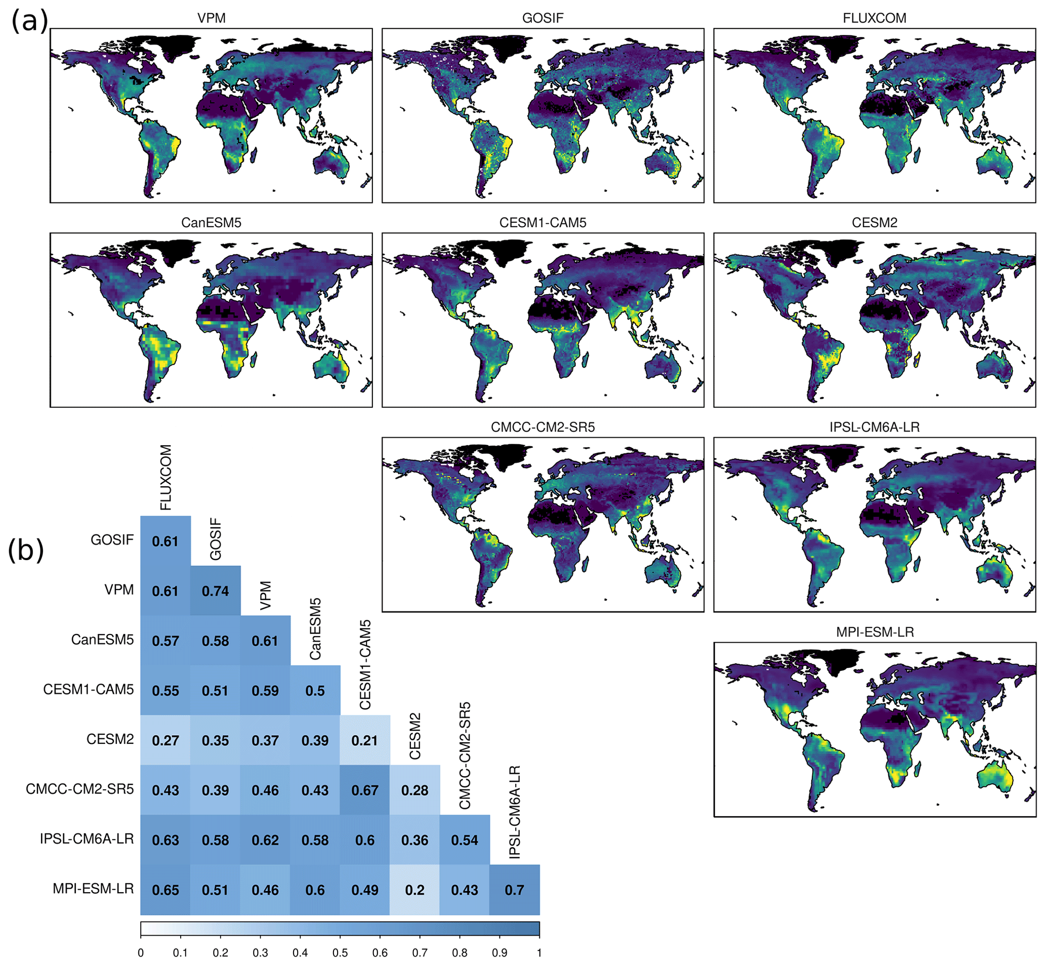
Figure 3 GPP IAV in three observational products (VPM, GOSIF, and FLUXCOM) and six ESMs. Panel (a) presents the spatial patterns of GPP IAV, with brighter colours representing higher values. The data are scaled across ESMs to highlight differences in patterns and not absolute differences. Panel (b) displays the spatial correlations between the products.

Because we focus on the spatial patterns of IAV rather than absolute differences, the GPP IAV patterns are scaled for better comparison (Fig. 3). We find agreement in the large-scale patterns of GPP IAV, with most of the IAV in the ESMs in the northern Amazon Basin and in the semi-arid tropics like western South America, southern Africa, South Asia, Australia, and southern North America (detailed maps of the location of the semi-arid regions in the ESMs are shown in Fig. 5). A closer examination of GPP IAV reveals that the ESMs show less agreement in the regions contributing most to the IAV, especially in the semi-arid tropics. Some ESMs have large hotspots of GPP IAV that cannot be found in other ESMs. These unique hotspots are the western Amazon Basin (CanESM5), central South America (CESM2), southern Africa (MPI-ESM-LR and CanESM5), and Australia (MPI-ESM-LR). We find the most consistency on the northern coast of South America, which is a high-IAV region in most ESMs. The spatial patterns of IAV have an average correlation of 0.47 among the ESMs. The ESM with the lowest correlation values is CESM2, with an average of 0.29. CESM2 stands out with a very low IAV in the tropical rainforests of the Amazon and Congo basins and in Southeast Asia.

The correlation among the observational products is 0.65; although these products confirm most of the IAV patterns of the ESMs, we find stronger deviations in South America. While many ESMs have IAV hotspots along the northern coast of South America, this is only reproduced in FLUXCOM. However, all observational products show a high GPP IAV in western South America, which can not be found in the ESMs. The spatial patterns of GPP IAV revealed here correspond to the literature, which suggests that the semi-arid tropics, tropical forests, grasslands, and croplands are the main drivers of global GPP IAV (Ahlström et al., 2015; Piao et al., 2020; O'Sullivan et al., 2020). These studies also reflect the large uncertainty in the contribution of the individual semi-arid regions to GPP IAV between the models, in particular the uncertain role of Australia. In an ensemble of eight LSMs, Australia contributed 39 %, semi-arid tropical Africa contributed 32 %, and Southeast Asia contributed 10 % to global GPP IAV, whereas temperate South America only contributed 2 % (Chen et al., 2017). Although Australia has the highest mean model IAV, the variability in IAV between the models is also the largest, with GPP IAV ranging between 0.26 and 1.01 Pg C yr⁻¹. While the large role of the dry tropics in driving GPP IAV is not disputed, it is likely that ESMs underestimate GPP IAV in wet tropical forests (O'Sullivan et al., 2020). This results from the limited availability of observations due to few flux towers and from the fact that the quality of remote-sensing products is limited in tropical forests due to saturation effects and a high cloud cover (Kolby Smith et al., 2016). In this study, the low GPP IAV in tropical forests is especially evident for CESM2, as IAV increases abruptly outside the wet tropical forests.

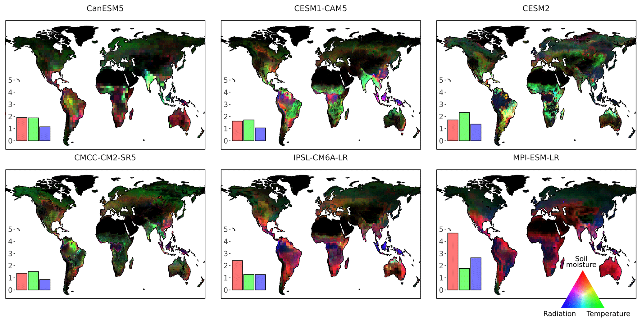
Figure 4 The contribution of environmental drivers to GPP variability ($\mathit{\sigma }{\mathrm{GPP}}_{\left(\mathrm{IAV}\right)}^{\mathrm{ENV}}$). Colour intensity represents higher GPP IAV. The data are scaled across ESMs to highlight differences in patterns, not absolute differences. Bars represent the mean contribution of environmental drivers to global GPP IAV ($\mathrm{kgC}{\mathrm{10}}^{-\mathrm{9}}{\mathrm{m}}^{-\mathrm{2}}{\mathrm{s}}^{-\mathrm{1}}$).

The divergence in GPP IAV across different ESMs is largely caused by three factors: the sensitivity of carbon fluxes to climatic drivers (Piao et al., 2020), as discussed in Sect. 3.2; phenology (Chen et al., 2017; Peano et al., 2019, 2021); and meteorological input (Anav et al., 2015). The role of phenology is crucial because the amount and quality of leaves determine the carbon fluxes between the land and the atmosphere (Peano et al., 2021). Most LSMs tend to have a better representation of the growing season type and growing season boundaries in the wet than in the semi-arid tropics. Peano et al. (2021) analysed the start and end months of growing seasons in eight LSMs under the same climate forcing and found several regions with a wide range of simulated growing seasons. The largest uncertainties in the growing season are in the semi-arid tropics, the same regions in which we find little agreement in GPP IAV. The start of the growing season ranges from February to October in Australia and from March to October in southern Africa, while the end of the growing season ranges from March to September in Africa between 0 and 15^∘ N. The vegetation types with the largest uncertainty in growing season timing are broadleaf, deciduous shrubs, which are mostly located in northern Australia; Southern Hemisphere crops; broadleaf, evergreen trees; and grasses. The better-performing LSMs have a high number of plant functional types or use more complex phenology schemes that depend on plant functional types, and they also use a larger number of environmental variables to constrain phenology. Its complex phenological scheme puts ORCHIDEE among the better-performing LSMs and might also explain the high correlation of IPSL-CM6A-LR with the GPP IAV for all three observational products.

A misrepresentation of phenology could also explain the overall high IAV in MPI-ESM-LR. JSBACH overestimates the seasonality of the LAI in the tropics, and this becomes visible in the strong seasonal cycle of tropical LAI in MPI-ESM-LR (Song et al., 2021). Consequentially, the area of the evergreen tropics is underestimated in JSBACH (Peano et al., 2021). This leads to a larger fraction of semi-arid tropics with a higher GPP IAV. This amplification of the equatorial dry season might lead to the high GPP IAV in the northern Amazon and contribute to the overall high IAV in MPI-ESM-LR (Wang et al., 2011).

3.2 Drivers of GPP IAV

To determine the drivers of GPP IAV, we analysed the sensitivity of GPP to environmental drivers using regression analysis. The globally averaged contribution of the drivers to GPP IAV is shown as the bars in Fig. 4. The CLM family and CanESM5 have similar patterns, with temperature dominating the IAV or being on par with soil moisture. IPSL-CM6A-LR and MPI-EMS-LR have distinctly different patterns, with soil moisture dominating the IAV and radiation contributing equally or more than temperature. A reason for the large contribution of soil moisture to GPP IAV in IPSL-CM6A-LR and MPI-ESM-LR could be that both ESMs are at the high end of soil moisture IAV for deep soil layers in the Southern Hemisphere (Qiao et al., 2022), where many of the semi-arid ecosystems are located that contribute most to GPP IAV. Another explanation could be that out of 11 ESMs, IPSL-CM6A-LR and MPI-ESM-LR have the lowest warm-season soil moisture (Padrón et al., 2022). This increase in dryness can lead to a larger extent of semi-arid ecosystems with a generally higher GPP IAV. Another effect of reduced warm-season soil moisture can be an increase in the land–atmosphere coupling strength (Santanello et al., 2018). Stronger land–atmosphere coupling would explain the higher correlation between soil moisture and temperature in IPSL-CM6A-LR and MPI-ESM-LR (Padrón et al., 2022) and would make the regression coefficients shift towards the stronger predictor, which is soil moisture.

The spatial drivers of GPP IAV show agreement in the wet and arid tropics, whereas there is little consistency in the semi-arid transition zones (Fig. 4). In many ESMs, the GPP IAV in the wet tropics and in eastern China is induced by radiation, while soil moisture becomes more prevalent along the aridity gradient and is driving IAV in southern Africa, southern South America, and Australia. The IAV in the remaining land surface is driven predominantly by soil moisture in IPSL-CM6A-LR and MPI-ESM-LR, whereas it is driven by a combination of temperature and soil moisture in the remaining ESMs.

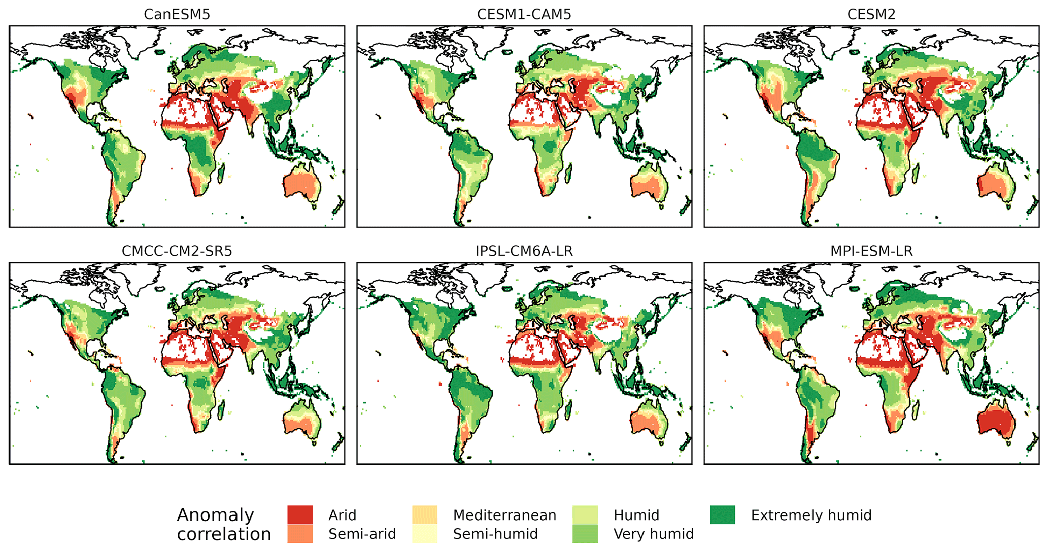
Figure 5 De Martonne aridity index of the analysed models.

Some of the differences in GPP sensitivity among the ESMs can be explained by differences in aridity. A higher sensitivity to soil moisture can result from a dryer climate. The distribution of climate zones in the analysed models is shown in Fig. 5 using the De Martonne aridity index (Gavrilov et al., 2019). MPI-ESM-LR and CanESM5 show an above-average extent of arid and semi-arid regions in Australia and southern Africa. This could explain the high sensitivity of GPP to soil moisture in these regions. Differences in climate also explain some of the discovered GPP patterns in the Amazon Basin. CESM2 is the model with the most humid climate in the Amazon Basin, which could be the reason for the low sensitivity of GPP to soil moisture and the generally low GPP IAV in this region. In contrast, we find that CanESM5 is on the other side of the spectrum, with a relatively dry Amazon Basin, leading to a higher sensitivity to soil moisture and a high GPP IAV. However, there are also differences in GPP sensitivity that cannot be explained by differences in climate. IPSL-CM6A-LR is more or equally humid in Australia, southern Africa, and South America than the models of the CLM family, despite having a high sensitivity of GPP to soil moisture in these regions. These differences are more likely to be caused by differences in their land surface models than by climate.

The general patterns of GPP sensitivity agree with reported sensitivity patterns in the literature. Multi-model averages and observations of GPP sensitivity agree with the larger role of temperature in tropical forests, radiation in western Amazonia, and the importance of precipitation in the semi-arid tropics (O'Sullivan et al., 2020; Anav et al., 2015). However, the role of water on carbon fluxes increases when soil moisture is used instead of precipitation in sensitivity studies (Piao et al., 2020). This can be observed in the sensitivity of net biome productivity (NBP), which shows a more balanced contribution of soil moisture and temperature in the wet tropical forests (Piao et al., 2020; Padrón et al., 2022). Although the comparison of GPP and NBP imposes limitations, GPP explains the majority of tropical NBP (Ahlström et al., 2015). This suggests that the low water sensitivity of tropical GPP might explain the lower than expected GPP IAV in tropical forests in ESMs.

3.3 Predictability of GPP

To analyse the role of GPP in the predictability of atmospheric CO₂, we assessed GPP predictability using two metrics. The predictable component (pc) is calculated as the difference between ensemble variability and IAV and provides a measure of absolute predictable variability. The pc can be used to assess the predictability of GPP fluxes that contribute to CO₂ variability. The predictable fraction (pf) is the ratio of pc to IAV and illustrates how well memory is retained in the system. This metric can be used to compare the predictive performance of different biomes, for example.

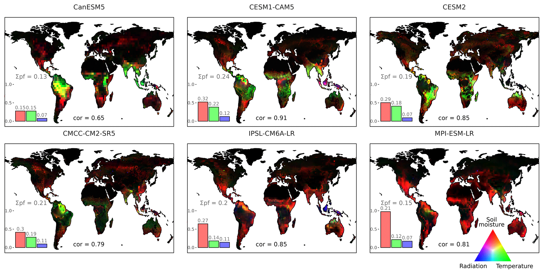
Figure 6 The contribution of environmental drivers to the predictable component (pc) of GPP. The contribution is calculated as the difference between the IAV and the ensemble variability within lead year 1 of the hindcast experiments. Values are scaled for each ESM. Bars represent the mean contribution of environmental drivers to the pc (Δσ GPP, in $\mathrm{kgC}{\mathrm{10}}^{-\mathrm{9}}{\mathrm{m}}^{-\mathrm{2}}{\mathrm{s}}^{-\mathrm{1}}$). Numbers on top of the bars show the predictable fraction (pf), which is the share of the pc to overall IAV. The correlation between GPP IAV and the pc is shown at the bottom of the plots.

There is relatively high consistency among the pf values of the environmental drivers across the models (pf^{Soil moisture} > pf^Temperature > pf^Radiation; the numbers above the bars in Fig. 6). This pattern reflects the anticipated differences in predictability among the drivers. Atmospheric fields, as radiation, have a low persistence, leading to a low predictability of 2 weeks for most regions (Zeng et al., 2008). Soil hydrology, on the other hand, acts as a low-pass filter that removes the unpredictable high-frequency variability in precipitation and allows a predictability of soil moisture of around 2 years (Chikamoto et al., 2017). Temperature gains most of its predictability through sea surface temperature (SST) forcing in the equatorial regions (Feng et al., 2011) and via land–atmosphere coupling in the semi-arid tropics (Seo et al., 2019).

The overall pf of CESM2, CMCC-CM2-SR5, and IPSL-CM6A-LR falls into a narrow window of 0.19 to 0.21. CESM1-CAM5 has the highest pf with a value of 0.24. It is likely that this increased share of predictable IAV is not due to differences in model structure but rather due to the large number of ensemble members (40). Most other ESMs in this study have only 10 ensemble members, which is not enough to capture the difference between ensemble variance and IAV; thus, an increase in ensemble members leads to an increase in prediction skill (Meehl et al., 2021). However, despite having 20 ensemble members, CanESM5 has the lowest pf among the models. A possible explanation could be the low IAV in deep-layer soil moisture in CanESM5 (Qiao et al., 2022). A limited ability to reproduce the full spectrum of soil moisture variability could mean that the soils have a smaller buffering capacity. As a result, they are not able to simulate the observed persistence of soil moisture anomalies, leading to a reduction in predictability. On the other hand, a high variability in soil moisture does not guarantee a high pf, as seen, for example, for MPI-ESM-LR. The low pf of MPI-ESM-LR can be explained by the sensitivity of GPP to radiation. As only 7 % to 12 % of the radiation-induced IAV is predictable, a high share of σGPP^Radiation reduces the predictability of GPP. This becomes evident in MPI-ESM-LR, in which the share of σGPP^Radiation is 20 % higher than in the other ESMs.

We find that the regions contributing to the predictability of atmospheric CO₂ (pc) are highly related to the IAV patterns. The spatial correlation between pc and IAV exceeds 0.79 in all models except CanESM5. Indeed, these high correlations between predictability and IAV align with our understanding. Under a constant pf, pc would grow linearly with increasing IAV, leading to a perfect correlation. These high correlations show that the differences in the predictability of atmospheric CO₂ are determined more by the differences in GPP IAV than the differences in the pf of GPP. While the pf values show that the ESMs have a similar degree of memory retention, there are few overlaps in the spatial distribution of the pc, with an average correlation of 0.38 between the ESMs. For an alternative quantification of this disagreement, we separate the high-predictability grid cells, which are the grid cells contributing to the top 20th quantile of pc. A total of 74 % of these high-predictability grid cells are unique to only one ESM, and only 8 % of high-predictability grid cells can be found in three or more ESMs.

Although the spatial patterns of the pc broadly resemble the patterns of GPP IAV, there are some slight differences between these fields. The pc is relatively high along the northeastern coast of South America in most ESMs. This could be due to the high climate predictability caused by slowly evolving Atlantic SST patterns (Dirmeyer et al., 2018). Other systematic differences can be explained by the differing pc of the environmental drivers. The most evident is the difference between IAV and predictability in regions where GPP IAV is driven by radiation. This leads to relatively low predictability in the tropical rainforests of the western Amazon Basin and the Congo Basin. An exception is the predictability provided through radiation on the Southeast Asian islands in IPSL-CM6A-LR and CESM1-CAM5. High predictability in these regions could be explained by the proximity to the ENSO SST region. Strong and predictable SST anomalies in the tropical Pacific that surround the islands can directly influence the cloud cover over land. The predictable component is also higher over areas where IAV is driven by soil moisture rather than temperature. In many ESMs, this leads to a high predictable component in the semi-arid regions of South America, Africa, and India.

4 Conclusions

We tested the ability of six ESMs to predict terrestrial GPP and determined their similarities and the sources of uncertainties. The ESMs are fairly similar in their ability to retain memory in hindcast simulations and predict their own variability, with the pf values of four of the ESMs falling between 19 % and 24 %. Most of the GPP pf is provided by soil moisture. Up to 32 % of the GPP IAV caused by soil moisture is predictable, whereas this value is only 7 % to 12 % for the IAV caused by radiation. The differences in the pf values among ESMs are due to the ensemble size and the sensitivity of GPP to radiation. Further sources of predictability that are not studied here are long-term vegetation dynamics. Specifically, the large and structural changes like tree mortality (Wigneron et al., 2020) and recruitment (Holmgren et al., 2001). These processes only occur in extreme years and cause shifts in ecosystem states with long-lasting effects. The correct representation of these processes in ESMs allows them to reproduce the low-frequency IAV in vegetation, thereby extending the pf of GPP.

Although ESMs are similar in the fraction of GPP IAV that they can predict, there are substantial differences in the patterns and drivers of GPP IAV. The ESMs have distinct, non-overlapping hotspots of GPP IAV that drive the variability in atmospheric CO₂. We find large disparities in the role of Australia, southern Africa, and central South America in GPP IAV. The leading cause of the uncertainties in IAV patterns are differences in the response of GPP to soil moisture and the capability of the ESMs to simulate soil hydrology accurately. These differences materialize through the direct effect of soil moisture on photosynthesis and through the role of soil moisture on phenology. The inability of ESMs to reproduce GPP IAV also means that there are regions where the potential predictability of GPP does not resemble the actual predictive skill.

This study shows that the predictability of atmospheric CO₂ is currently not limited by the processes that provide predictability in the Earth system but rather by the representation of carbon flux variability patterns. The mismatches in GPP IAV imply that the IAV in atmospheric CO₂ is caused by different regions and by different drivers across the ESMs. Consequentially, when ESMs predict the atmospheric CO₂, the GPP anomalies that constitute the predicted CO₂ growth rate originate from different regions. Because the predicted CO₂ depends more on the distribution of GPP IAV hotspots than actual mechanisms that provide predictability, CO₂ forecast skill is not a suitable metric for studies on carbon flux predictability. An ESM with a high carbon flux predictability can be outperformed with respect to CO₂ forecast skill by a model that has a better representation of IAV patterns. A more suitable measure to assess carbon flux predictability could be the globally averaged anomaly correlation coefficient.

With the current uncertainties in GPP IAV patterns, the prediction of atmospheric CO₂ relies less on the prediction of regional climate anomalies and more on the predictable global climate patterns like ENSO. These global climate anomalies are able to balance out the regional differences in GPP IAV patterns by affecting large parts of the land surface simultaneously. In order to utilize the benefits of regional climate predictability for the predictability of CO₂, further work ought to focus on constraining GPP IAV and not on the processes providing predictability. The most limiting aspect in the use of ESMs to predict atmospheric CO₂ is a better understanding of the drivers of carbon flux variability. Whether GPP is limited by moisture, temperature, or radiation does not only affect variability patterns but also the predictability of the fluxes. An overestimation of humidity in an ecosystem by an ESM would result in GPP being more controlled by radiation than soil moisture, leading to an underestimation of predictability (or vice versa for systems that are too dry).

The findings of this study also suggest that previous estimations of ESM-based CO₂ forecast skill are underestimating the predictive capabilities of these systems. Various post-processing strategies could help to produce a CO₂ forecast skill that is not obscured by inaccurate IAV patterns but is a closer representation of the actual performance of ESM-based prediction systems. These strategies could include the scaling of carbon flux IAV patterns to resemble the observed IAV patterns. As there are strong regional differences in the predictive performance among the ESMs, another strategy would be to combine ESM predictions in a way that utilizes these differences. This could be done in a regionally weighted multi-model approach.

The limiting factor to predicting atmospheric CO₂ is the chaotic nature of weather and climate. However, our results show that we have not reached this limitation yet and that we are instead constrained by our understanding of terrestrial carbon flux variability. The development of observational products for terrestrial carbon fluxes, especially in the tropics, remains the main objective on the path of improving the predictability of the global carbon cycle and atmospheric CO₂.