Carbon cycle feedbacks in an idealized simulation and a scenario simulation of negative emissions in CMIP6 Earth system models

Limiting global warming to well below 2 ^∘C by the end of the century is an ambitious target that requires immediate and unprecedented emission reductions. In the absence of sufficient near-term mitigation, this target will only be achieved by carbon dioxide removal (CDR) from the atmosphere later during this century, which would entail a period of temperature overshoot. Aside from the socio-economic feasibility of large-scale CDR, which remains unclear, the effects on biogeochemical cycles and climate are key to assessing CDR as a mitigation option. Changes in atmospheric CO₂ concentration and climate alter the CO₂ exchange between the atmosphere and the underlying carbon reservoirs of the land and the ocean. Here, we investigate carbon cycle feedbacks under idealized and more realistic overshoot scenarios in an ensemble of Earth system models. The responses of oceanic and terrestrial carbon stocks to changes in atmospheric CO₂ concentration and changes in surface climate (the carbon–concentration feedback and the carbon–climate feedback, quantified by the feedback metrics β and γ, respectively) show a large hysteresis. This hysteresis leads to growing absolute values of β and γ during phases of negative emissions. We find that this growth over time occurs such that the spatial patterns of feedbacks do not change significantly for individual models. We confirm that the β and γ feedback metrics are a relatively robust tool to characterize inter-model differences in feedback strength since the relative feedback strength remains largely stable between phases of positive and negative emissions and between different simulations, although exceptions exist. When the emissions become negative, we find that the model uncertainty (model disagreement) in β and γ increases more strongly than expected from the assumption that the uncertainties would accumulate linearly with time. This indicates that the model response to a change from increasing to decreasing forcing introduces an additional layer of uncertainty, at least in idealized simulations with a strong signal. We also briefly discuss the existing alternative definition of feedback metrics based on instantaneous carbon fluxes instead of carbon stocks and provide recommendations for the way forward and future model intercomparison projects.

1 Introduction

Estimated remaining carbon budgets compatible with limiting anthropogenic warming to 1.5 or 2 ^∘C above pre-industrial levels are extremely tight and will be exhausted within the next few years if the current emission rate is maintained (e.g., Rogelj et al., 2015; Goodwin et al., 2018; Masson-Delmotte et al., 2018; Forster et al., 2023; Smith et al., 2023). Therefore, unless CO₂ emissions are reduced immediately at an unprecedented rate, the 1.5 or 2 ^∘C targets can only be reached after a period of temperature overshoot (Rogelj et al., 2015; Ricke et al., 2017; Geden and Löschel, 2017; Riahi et al., 2021). Although the option to remove large quantities of carbon from the atmosphere remains speculative (Gasser et al., 2015; Larkin et al., 2018; Fuss et al., 2018; Creutzig et al., 2019; Smith et al., 2023), in such overshoot pathways, excessive near-term carbon emissions would be compensated for by large-scale carbon dioxide removal (CDR) later in this century. Research on negative emissions exploring the reversibility of CO₂-induced climate change has been conducted for more than a decade (e.g., Boucher et al., 2012; Wu et al., 2015; Tokarska and Zickfeld, 2015; Li et al., 2020; Jeltsch-Thömmes et al., 2020; Yang et al., 2021; Schwinger et al., 2022; Bertini and Tjiputra, 2022). These studies generally report a hysteretic behavior of the Earth system under negative emission, resulting in greatly varying reversibility for different aspects of the Earth system. While the surface temperature trend follows a reduction in atmospheric CO₂ relatively closely (e.g., Boucher et al., 2012; Jeltsch-Thömmes et al., 2020), the hysteresis can be large in the interior ocean, making, for example, rises in the ocean heat content and steric sea level as well as interior ocean oxygen content changes and acidification largely irreversible on policy-relevant timescales (Mathesius et al., 2015; Li et al., 2020; Schwinger et al., 2022; Bertini and Tjiputra, 2022). The same is true for the loss of carbon from thawing permafrost soils (MacDougall et al., 2015; Gasser et al., 2018; Park and Kug, 2022; Schwinger et al., 2022).

Carbon emissions drive multiple responses of the Earth system via changes in its physical climate and the biogeochemical carbon cycle. Under increasing atmospheric CO₂ concentrations, increasing carbon uptake by the ocean and terrestrial biosphere slows down global climate change by removing the greenhouse gas CO₂ from the atmosphere, a process that is mainly driven by the dissolution of CO₂ into the oceans (e.g., Revelle and Suess, 1957; Siegenthaler and Oeschger, 1978) and the CO₂ fertilization effect on the terrestrial biosphere (Schimel et al., 2015). On the other hand, Earth system model (ESM) simulations show that this carbon uptake is reduced by progressive global warming due to, among others, changes in ocean circulation, a reduction in CO₂ solubility in warmer waters, increased respiration rates from soils (Tharammal et al., 2019; Arora et al., 2020; Canadell et al., 2021), and carbon release from degrading permafrost. These two feedback processes – the response to rising CO₂ concentrations and the response to climate change – are termed the carbon–concentration feedback and the carbon–climate feedback, respectively (Gregory et al., 2009). In the context of overshoot pathways, carbon cycle feedbacks determine the efficiency of negative emissions, as the oceans and the terrestrial biosphere will first take up carbon at reduced rates but will eventually turn into sources of carbon for the atmosphere (Jones et al., 2016a; Schwinger and Tjiputra, 2018).

The carbon–concentration and carbon–climate feedbacks can be characterized by feedback metrics; for example, by the feedback factors β and γ (Friedlingstein et al., 2003) that quantify the gain/loss of carbon in terrestrial or marine reservoirs per unit change in atmospheric CO₂ concentration and temperature, respectively (see Sect. 2 for details). These feedback factors are valuable tools to compare the feedback strength among different models (Friedlingstein et al., 2003, 2006; Yoshikawa et al., 2008; Boer and Arora, 2009; Gregory et al., 2009; Roy et al., 2011; Arora et al., 2013, 2020) and can be calculated using idealized model simulations in which the effect of CO₂ on the carbon cycle and the radiative effect of CO₂ are decoupled. In a biogeochemically coupled (BGC) simulation, the radiation code of an ESM does not respond to increasing atmospheric CO₂ concentrations but the terrestrial and marine carbon cycles do. There is little climate change in such a simulation, which can therefore be used to quantify the carbon–concentration feedback. The difference between a standard (fully coupled, COU) simulation and the BGC simulation is used to quantify the carbon–climate feedback. In the last two phases of the Coupled Model Intercomparison Project (CMIP5 and CMIP6, Taylor et al., 2012; Eyring et al., 2016), carbon cycle feedbacks were addressed by conducting additional decoupled simulations of the standard 1 % CO₂ simulation which prescribes an increase in atmospheric CO₂ of 1 % yr⁻¹ until the concentration has quadrupled (Arora et al., 2013, 2020). Next to this idealized simulation, the protocol for the CMIP6 Coupled Climate–Carbon Cycle Model Intercomparison Project (C4MIP, Jones et al., 2016b) also proposes a BGC simulation for the SSP5-3.4-OS (hereafter “ssp534-over”) scenario (O'Neill et al., 2016). This scenario describes an overshoot pathway in which emissions increase unmitigated until 2040 but strong mitigation (including CDR) is undertaken thereafter. In contrast to the 1 % CO₂ simulation, where no forcing other than atmospheric CO₂ is varied, the quantification of feedbacks in this scenario simulation is complicated by the presence of land-use change and changes in radiative forcing through the emissions of aerosols and non-CO₂ greenhouse gasses (Melnikova et al., 2021, 2022).

One open question regarding carbon cycle feedbacks under negative emissions is the state against which the feedbacks should be measured. A sensible definition requires that any gain or loss of carbon is calculated relative to a state where the carbon cycle is in equilibrium. Schwinger and Tjiputra (2018) opted to keep the pre-industrial state as the reference after the onset of negative emissions. We follow this approach here, but we note that Chimuka et al. (2023) recently proposed an alternative approach which defines the feedbacks during the negative emission phase relative to the state at the onset of negative emissions. Since the Earth system will be in disequilibrium at this point in time, this approach requires an additional simulation that allows the lagged response of the Earth system to this disequilibrium to be estimated and removed.

Permafrost soils in the northern high latitudes have accumulated roughly 1100–1700 Pg of carbon in the form of frozen organic matter – about twice as much as currently contained in the atmosphere (Hugelius et al., 2014; Schuur et al., 2015). The release of CO₂ and methane (CH₄) from thawing permafrost will amplify global warming due to anthropogenic emissions and further accelerate permafrost degradation and microbial decomposition (Feng et al., 2020; Smith et al., 2022). This positive feedback and the fact that Arctic temperatures are increasing at a much faster rate than the global average (Liang et al., 2022; Rantanen et al., 2022) have caused permafrost to be considered among the key tipping elements of the climate system, although permafrost degradation may not be an abrupt (albeit irreversible) process (Armstrong McKay et al., 2022; Yokohata et al., 2020; Lenton et al., 2019). A temporary temperature overshoot might entail important legacy effects, as high-latitude ecosystems and the state of permafrost-affected soils take several centuries to adjust to the new atmospheric conditions (de Vrese and Brovkin, 2021). Current-generation ESMs are still in their infancy when it comes to representing the complex and often small-scale processes of permafrost carbon degradation. Here we take advantage of the fact that one of the CMIP6 ESMs considered in this study has a vertically resolved representation of soil carbon, which enables us to estimate the contribution of permafrost degradation to the total carbon–climate feedback for this model.

Except for the recent studies by Schwinger and Tjiputra (2018), Melnikova et al. (2021, 2022), and Chimuka et al. (2023), all previous studies that quantify the carbon–concentration and carbon–climate feedbacks are based on ESM simulations with increasing atmospheric CO₂. Here, we take advantage of a simulation conducted for the CMIP6 Carbon Dioxide Removal Model Intercomparison Project (CDRMIP, Keller et al., 2018) that mirrors the 1 % CO₂ simulation by prescribing a decrease in atmospheric CO₂ of 1 % yr⁻¹. For simplicity, we refer to these two simulations as “1pctCO2-cdr” in the following text. We complement this simulation with a BGC simulation (1pctCO2-cdr-bgc) to quantify, in a manner consistent with previous feedback studies (Arora et al., 2013, 2020), the carbon–concentration and carbon–climate feedbacks under negative emissions in an ensemble of CMIP6 ESMs. We complement these previous studies with a spatial analysis of feedback patterns, and we compare the feedbacks from the positive and negative emission phases of the 1pctCO2-cdr simulation to the feedbacks obtained from the ssp534-over scenario. For the latter, land-use change has been shown to have a dominant effect over the carbon–concentration or carbon–climate feedbacks by Melnikova et al. (2021, 2022), and these authors present a more detailed analysis of the role of land-use change in the ssp534-over scenario. Since land-use change is not a feedback process, we focus in this study on regions that are not dominated by agricultural areas when comparing feedbacks between the ssp534-over and 1pctCO2-cdr simulations.

The purpose of this study is to investigate the evolution of carbon cycle feedbacks and their uncertainty under the deployment of negative emissions. Since feedback metrics are known to depend on the emission (or concentration) pathway, we compare the relative feedback strength and the spatial patterns of feedbacks between positive and negative emission phases as well as between idealized and scenario simulations. We also briefly explore the contribution of permafrost carbon losses to the carbon–climate feedback and the impact of alternative feedback metric definitions that rely on instantaneous carbon fluxes rather than carbon stocks in the context of negative emissions.

2 Description of feedback metrics, simulations, and models

2.1 Carbon cycle feedback metrics

The sensitivity of the carbon cycle to changes in atmospheric CO₂ concentration ([CO₂]) and its sensitivity to changes in physical climate can be measured using two feedback metrics, which can be based on either changes in carbon stocks (as introduced by Friedlingstein et al., 2003) or instantaneous carbon fluxes (as introduced by Boer and Arora, 2009). Changes in carbon stocks are equivalent to the time-integrated carbon fluxes across the air–land and air–sea interfaces, such that, for the approach used by Friedlingstein et al. (2003) (referred to as the integrated flux-based approach), the two feedback metrics are as follows:

1. β (PgC ppm⁻¹), which quantifies the strength of the carbon–concentration feedback, i.e., the changes in oceanic and terrestrial carbon stocks (ΔC_L,O) in response to changes in the atmospheric CO₂ concentration (Δ[CO₂]), and

2. γ (PgC ^∘C⁻¹), which measures the strength of the carbon–climate feedback, i.e., the changes in land and ocean carbon stocks (ΔC_L,O) in response to changes in the global average surface temperature (ΔT), where ΔT serves as a proxy for climate change.

Carbon feedback analysis requires, in addition to a standard fully coupled (COU) simulation, a biogeochemically (BGC) coupled simulation. In a BGC simulation, atmospheric [CO₂] is kept constant at its pre-industrial values for the radiative transfer calculations to isolate the response of land and ocean biogeochemistry to rising [CO₂] in the absence of CO₂-induced climate change. Using this pair of simulations (COU and BGC) results in the following expressions for β and γ (see Schwinger et al., 2014 for a derivation):

$$\begin{array}{}\text{(1)}& {\displaystyle }\begin{array}{rl}{\mathit{\beta }}_X=& {\displaystyle \frac{\mathrm{1}}{\mathrm{\Delta }\left[{\mathrm{CO}}_{\mathrm{2}}\right]}}\left({\displaystyle \frac{\mathrm{\Delta }{\mathrm{C}}_X^{\text{BGC}}\mathrm{\Delta }{T}^{\text{COU}}-\mathrm{\Delta }{\mathrm{C}}_X^{\text{COU}}\mathrm{\Delta }{T}^{\text{BGC}}}{\mathrm{\Delta }{T}^{\text{COU}}-\mathrm{\Delta }{T}^{\text{BGC}}}}\right)\\ \simeq & {\displaystyle \frac{\mathrm{\Delta }{\mathrm{C}}_X^{\text{BGC}}}{\mathrm{\Delta }\left[{\mathrm{CO}}_{\mathrm{2}}\right]}}\end{array}\text{(2)}& {\displaystyle }{\mathit{\gamma }}_X={\displaystyle \frac{\mathrm{\Delta }{\mathrm{C}}_X^{\text{COU}}-\mathrm{\Delta }{\mathrm{C}}_X^{\text{BGC}}}{\mathrm{\Delta }{T}^{\text{COU}}-\mathrm{\Delta }{T}^{\text{BGC}}}}\simeq {\displaystyle \frac{\mathrm{\Delta }{\mathrm{C}}_X^{\text{COU}}-\mathrm{\Delta }{\mathrm{C}}_X^{\text{BGC}}}{\mathrm{\Delta }{T}^{\text{COU}}}},\end{array}$$

where X can be either L for land or O for ocean. Although there is no change in the radiative forcing of CO₂ in the BGC simulation (such that we could expect ΔT^BGC=0), the surface temperature can vary due to changes in other radiative forcing agents (aerosols and non-CO₂ greenhouse gasses). Even in the idealized 1pctCO2-cdr simulation, where CO₂ is the only variable forcing, there are some climatic changes over the land surface due to a reduction in latent heat fluxes associated with stomatal closure at higher CO₂ levels, as well as changes in vegetation structure, coverage, and composition (Arora et al., 2020), which result in a small temperature increase along with changes in precipitation and soil moisture. The assumption of ΔT^BGC=0 will simplify Eqs. (1) and (2) such that the rightmost term holds. However, the results presented here are calculated using the complete expressions for β and γ (without the assumption ΔT^BGC=0) unless otherwise noted. For comparison, we also provide feedback factors calculated using the simplified (rightmost) definitions of β and γ in some figures. The instantaneous flux-based approach is equivalent to Eqs. (1) and (2) except that the deviations of the carbon pools ΔC_X are replaced by the instantaneous air–sea or air–land carbon fluxes F_X. To distinguish these feedback metrics from the integrated flux-based ones, the capital Greek letters B and Γ are used to denote them. The units of B and Γ are PgCyr⁻¹ppm⁻¹ and PgCyr^−1 ∘C⁻¹, respectively.

By combining Eqs. (1) and (2) to yield

$$\begin{array}{}\text{(3)}& {\mathit{\beta }}_X={\displaystyle \frac{\mathrm{1}}{\mathrm{\Delta }\left[{\mathrm{CO}}_{\mathrm{2}}\right]}}\left(\mathrm{\Delta }{\mathrm{C}}_X^{\text{BGC}}-{\mathit{\gamma }}_X\mathrm{\Delta }{T}^{\text{BGC}}\right),\end{array}$$

it can be seen that, in order to calculate β_X, the carbon stock changes in the biogeochemically coupled simulation are corrected for global mean temperature changes using γ_X. Hence, temperature changes in the biogechemically coupled simulation are fully accounted for as long as the underlying assumption of linearity holds. However, this assumption might be problematic, for example, if the spatial pattern of warming in a biogeochemically coupled scenario simulation arising from non-CO₂ forcings is very different from the warming patterns in the fully coupled simulation, particularly if the sign of the local temperature change is different from the global average (e.g., local cooling vs. global average warming). Such effects could become important at regional to local scales and will be discussed in Sect. 3.4.

It is worth mentioning that these feedback frameworks should be seen as a technique for assessing the relative sensitivities of models and understanding their differences (i.e., the model uncertainty of the estimated feedbacks), rather than as absolute measures of invariant system properties (Gregory et al., 2009; Ciais et al., 2013). The values of carbon cycle feedback metrics can vary over time within a model simulation (e.g., Arora et al., 2013) or between different scenarios (Hajima et al., 2014).

To gain insight into the reasons for differing responses among models, we apply the decomposition of the simplified expression for β_L (Eq. 1, assuming ΔT^BGC=0) following Arora et al. (2020). This allows us to investigate the contributions from different processes to changes in vegetation and soil carbon reservoirs (ΔC_V and ΔC_S, respectively):

$$\begin{array}{}\text{(4)}& \begin{array}{rl}{\mathit{\beta }}_{\text{L}}=& {\displaystyle \frac{\mathrm{\Delta }{\mathrm{C}}_{\text{L}}^{\text{BGC}}}{\left[{\mathrm{CO}}_{\mathrm{2}}\right]}}={\displaystyle \frac{\mathrm{\Delta }{\mathrm{C}}_{\text{V}}^{\text{BGC}}+\mathrm{\Delta }{\mathrm{C}}_{\text{S}}^{\text{BGC}}}{\left[{\mathrm{CO}}_{\mathrm{2}}\right]}}\\ =& \left({\displaystyle \frac{\mathrm{\Delta }{\mathrm{C}}_{\text{V}}^{\text{BGC}}}{\mathrm{\Delta }{\text{NPP}}^{\text{BGC}}}}{\displaystyle \frac{\mathrm{\Delta }{\text{NPP}}^{\text{BGC}}}{\mathrm{\Delta }{\text{GPP}}^{\text{BGC}}}}{\displaystyle \frac{\mathrm{\Delta }{\text{GPP}}^{\text{BGC}}}{\left[{\mathrm{CO}}_{\mathrm{2}}\right]}}\right)\\ +& \left({\displaystyle \frac{\mathrm{\Delta }{\mathrm{C}}_{\text{S}}^{\text{BGC}}}{\mathrm{\Delta }{R}_{\text{h}}^{\text{BGC}}}}{\displaystyle \frac{\mathrm{\Delta }{R}_{\text{h}}^{\text{BGC}}}{\mathrm{\Delta }{\text{LF}}^{\text{BGC}}}}{\displaystyle \frac{\mathrm{\Delta }{\text{LF}}^{\text{BGC}}}{\left[{\mathrm{CO}}_{\mathrm{2}}\right]}}\right)\\ =& {\mathit{\tau }}_{\text{cveg}\mathrm{\Delta }}{\text{CUE}}_{\mathrm{\Delta }}{\displaystyle \frac{\mathrm{\Delta }{\text{GPP}}^{\text{BGC}}}{\left[{\mathrm{CO}}_{\mathrm{2}}\right]}}\\ +& {\mathit{\tau }}_{\text{csoil}\mathrm{\Delta }}{\displaystyle \frac{\mathrm{\Delta }{R}_{\text{h}}^{\text{BGC}}}{\mathrm{\Delta }{\text{LF}}^{\text{BGC}}}}{\displaystyle \frac{\mathrm{\Delta }{\text{LF}}^{\text{BGC}}}{\left[{\mathrm{CO}}_{\mathrm{2}}\right]}}.\end{array}\end{array}$$

ΔNPP, ΔGPP, ΔR_h, and ΔLF represent the deviations of the net primary productivity, gross primary productivity, heterotrophic respiration, and litterfall flux, respectively, from their pre-industrial values. The terms τ_cvegΔand τ_csoilΔ are the turnover times (in years) of carbon in the vegetation and litter plus soil pools. $\frac{\mathrm{\Delta }\text{NPP}}{\mathrm{\Delta }\text{GPP}}$ is a measure of carbon use efficiency for the fraction of GPP (above its pre-industrial value) that turned into NPP after subtracting autotrophic respiration losses (denoted as CUE_Δ). $\frac{\mathrm{\Delta }\text{GPP}}{\left[{\mathrm{CO}}_{\mathrm{2}}\right]}$ (PgC yr⁻¹ ppm⁻¹) and $\frac{\mathrm{\Delta }{R}_{\text{h}}}{\mathrm{\Delta }\text{LF}}$ are a measure of the global CO₂ fertilization effect and the increase in heterotrophic respiration per unit increase in litterfall rate, respectively. Also, $\frac{\mathrm{\Delta }\text{LF}}{\left[{\mathrm{CO}}_{\mathrm{2}}\right]}$ (PgC yr⁻¹ ppm⁻¹) measures the global increase in litterfall rate per unit increase in CO₂.

2.2 Model simulations

The 1 % CO₂ experiment is a highly idealized model experiment that prescribes a rate of increase in [CO₂] of 1 % yr⁻¹ from pre-industrial values until the concentration has quadrupled after 140 years. No other forcings are varied in this experiment, i.e., land use as well as non-CO₂ greenhouse gasses and aerosol concentrations are held constant at their pre-industrial levels. This experiment was performed using the first coupled atmosphere–ocean general circulation models in the late 1980s, and important climate metrics such as the transient climate response (TCR; Meehl et al., 2020) and the transient response to cumulative emissions (TCRE; e.g., Gillett et al., 2013) are formally defined through the 1pctCO2 simulation. Likewise, the C4MIP carbon cycle feedback analysis for the last two phases of CMIP (Arora et al., 2013, 2020) relied on this simulation. Given the importance of the 1 % CO₂ experiment, the CMIP6 CDRMIP protocol proposes an experiment that mirrors this simulation by starting from its endpoint at year 140 and decreasing the atmospheric CO₂ at a rate of 1 % yr⁻¹ until the pre-industrial [CO₂] is restored. This experiment is designed to investigate the response of the Earth system to carbon dioxide removal in an idealized fashion. As noted above, in this study we refer to the 1 % CO₂ simulation and the mirrored −1 % CO₂ CDRMIP simulation collectively as 1pctCO2-cdr for simplicity. We note that the implied rates of CDR in the 1pctCO2-cdr simulation are huge and not practically feasible. Also, there is a jump from very large positive to very large negative diagnosed emissions at the end of year 140, which is clearly unrealistic. To investigate carbon cycle feedbacks under CDR, we have complemented the 1pctCO2-cdr simulation with a biogeochemical coupled 1pctCO2-cdr-bgc simulation that starts from the endpoint of the 1pctCO2-bgc simulation at year 140.

The family of shared socioeconomic pathways (SSPs, O'Neill et al., 2014) are designed to represent different socio-economic futures that social, demographic, political, and economic developments could lead to. These narrative SSPs are the basis for a set of quantitative future scenarios, a selection of which are now being used as input for scenario simulations by the latest ESMs in the framework of the CMIP6 ScenarioMIP (O'Neill et al., 2016). The ssp534-over scenario follows the high-emission SSP5-8.5 pathway until 2040, at which point strong mitigation policies are introduced to rapidly reduce emissions to zero by about 2070 and to net-negative levels thereafter (Fig. 3 of O'Neill et al., 2016). In contrast to the 1pctCO2-cdr simulation, the ssp534-over scenario includes land-use change as well as temporally varying forcing from aerosols and non-CO₂ greenhouse gasses throughout the simulation period (Fig. 1 of Liddicoat et al., 2021). For this study, we use the 1pctCO2-cdr and ssp534-over simulations from the CMIP6 archive together with the corresponding biogeochemically coupled simulations of these experiments. We note that the biogeochemically coupled 1pctCO2-cdr-bgc experiment is not part of CMIP6, but it is performed for this study by participating modeling groups.

The C4MIP simulation protocol does not allow us to separate carbon release (or uptake) through land-use changes from the carbon–concentration feedback, since land use is active in the biogeochemically coupled ssp534-over simulation. To focus on carbon cycle feedbacks, we eliminate the effect of land-use changes as much as possible by identifying regions that are mostly unaffected by human activity (referred to as “natural land”). To accomplish this in a way that the available CMIP6 output permits, we define natural land as grid cells with a maximum cropland fraction of less than 25 % at all time steps during the period 2015–2100. The threshold of 25 % used here for our heuristic approach is a compromise between accuracy (some signal of land-use change is still present) and spatial coverage (with increasingly lower thresholds, larger areas of the globe are excluded). Our results are not very sensitive to variations in the threshold between approximately 10 % and 30 %. Maps of maximum ssp534-over cropland fraction for each model (Fig. S1 in the Supplement) indicate that a 25 % threshold identifies hotspots of agricultural production reasonably well. To make our analysis comparable between the ssp534-over and 1pctCO2-cdr simulations, we also use the same set of grid cells for the 1pctCO2-cdr simulation (unless otherwise noted), even though land cover is not changed from its pre-industrial state in this simulation. We acknowledge that our approach does not explicitly address pasture grid cells or transitions from other land-use types to pasture. Nonetheless, in the ssp534-over scenario, a substantial expansion of bioenergy crops between 2040 and 2070 is assumed to replace pasture areas, while the area of land used as pasture remains relatively stable thereafter (see O'Neill et al., 2016). Hence, our approach, for this specific scenario, captures the majority of grid cells with transitions from pasture to cropland, while transitions from pasture to forest remain small.

2.3 Participating Earth system models

Table 1 summarizes the five ESMs that contributed to this study along with the experiments used for the analyses presented here. The primary features of these models are listed in Table 2 of Arora et al. (2020). MIROC-ES2L, NorESM2-LM (which employs version 5 of the Community Land Model, CLM5), and UKESM1-0-LL have a representation of the terrestrial nitrogen cycle implemented and coupled to their carbon cycle. Only the UKESM1-0-LL model has a land component that dynamically simulates vegetation cover and competition between their plant functional types (PFTs). Fire is included in the CNRM-ESM2-1 and NorESM2-LM models. NorESM2-LM is the only ESM with vertically resolved soil carbon, which allows the impact of warming on the carbon stored in permafrost soils to be studied in more detail. In this study, a grid cell was considered permafrost when the pre-industrial maximum active layer thickness was shallower than 3 m. A description and a comparison of the ocean biogeochemistry models used in the five ESMs can be found in the review by Seférian et al. (2020).

Table 1 List of the CMIP6 ESMs used in this study, the names of their biogeochemical component models, their resolutions, and the experimental variants used.

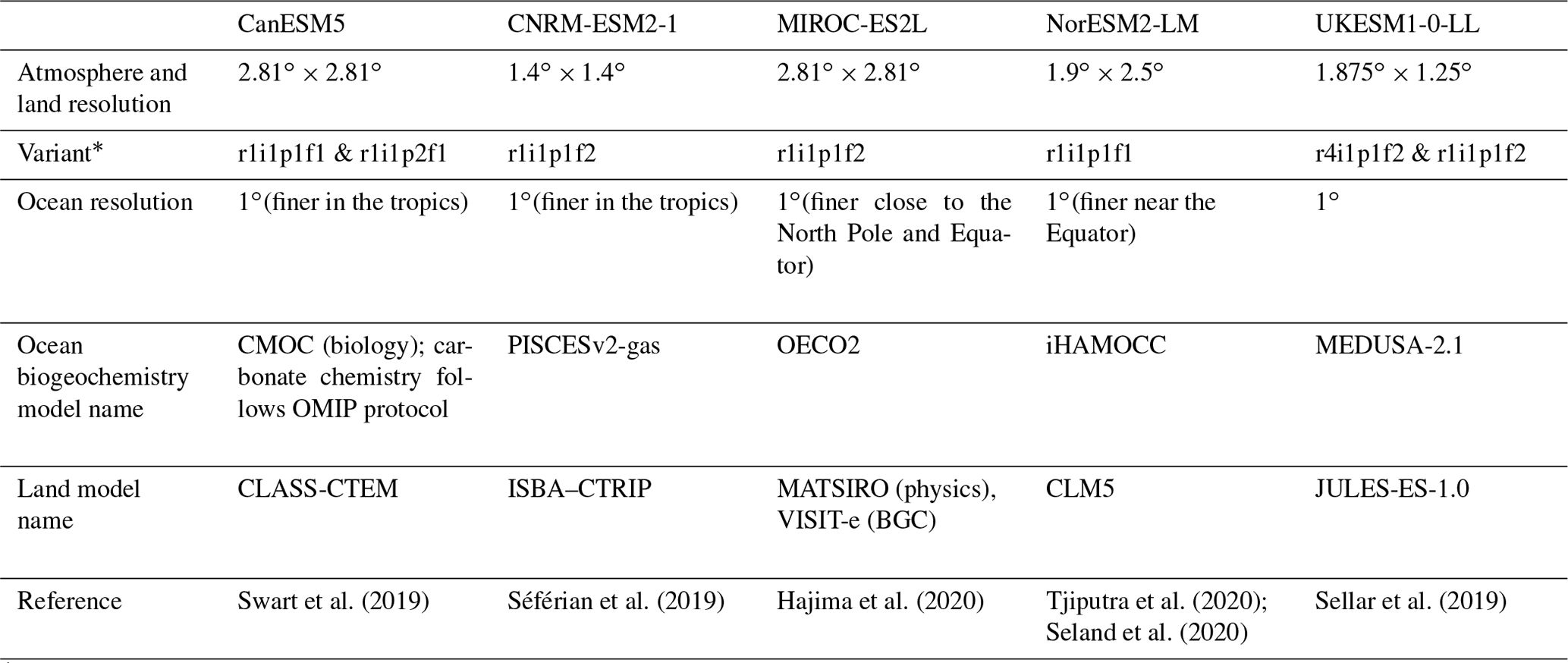
^∗ The CMIP6 experiment variant used across different simulations, including the piControl, historical, hist-bgc, ssp585, ssp585-bgc, ssp534-over, ssp534-over-bgc, 1pctCO2, 1pctCO2-bgc, 1pctCO2-cdr, and 1pctCO2-cdr-bgc experiments.

3 Results and discussion

3.1 Atmospheric CO₂, temperature, and carbon fluxes

The atmospheric CO₂ concentration ([CO₂]) for the concentration-driven ssp534-over scenario peaks at 571 ppm (a doubling of the pre-industrial CO₂ concentration) in the year 2062 and decreases to 497 ppm in 2100 (Fig. 1a). According to the scenario design (see O'Neill et al., 2016), strong mitigation policies (including the deployment of bioenergy with carbon capture and storage (BECCS) and other carbon dioxide removal technologies) start in 2040, resulting in an immediate decrease in the CO₂ growth rate, which peaks in 2041 (Fig. 1e). In the 1pctCO2-cdr simulation, the prescribed [CO₂] is symmetric around its 4×CO₂ peak of 1133 ppm in the year 140 (Fig. 1c). The rate of change in the CO₂ concentration (Fig. 1e) greatly differs between the ssp534-over and 1pctCO2-cdr experiments. In particular, the CO₂ growth rate in the idealized 1pctCO2-cdr experiment shows a sudden and large jump from positive to negative values at the transition from the ramp-up to the ramp-down phase.

The five participating ESMs show large differences in global mean surface air temperature change relative to pre-industrial values in the ssp534-over simulation (Fig. 1b). Peak temperatures vary from 2 ^∘C in NorESM2-LM to 4.35 ^∘C in CanESM5. The timing of the global surface air temperature peak varies from 2062 for the MIROC-ES2L and UKESM1-0-LL models to 2100 for CNRM-ESM2-1. After this peak, the temperature declines again (except for CNRM-ESM2-1), reaching end-of-the-century values that range from 1.39 ^∘C above pre-industrial in NorESM2-LM to 3.47 ^∘C in CanESM5. The multi-model mean global surface air temperature is 2.66 ^∘C at the end of the 21st century. The model-mean growth rate of the global surface air temperature (Fig. 1f) plateaus at about 0.05 ^∘C yr⁻¹ between approximately 2030–2050 before it starts to decline to below zero towards the end of the simulation.

Temperature changes in the BGC simulation of ssp534-over are not negligible since the non-CO₂ forcing agents as well as land-use change do evolve over time in this scenario, in contrast to the idealized 1pctCO2-cdr simulation. Positive peak temperature anomalies range from 0.37 ^∘C (CNRM-ESM2-1 in 2098) to 1.29 ^∘C (CanESM5 in 2057). UKESM1-0-LL also shows a pronounced negative temperature anomaly during the historical period of the BGC simulation of −0.80 ^∘C in the year 1990.

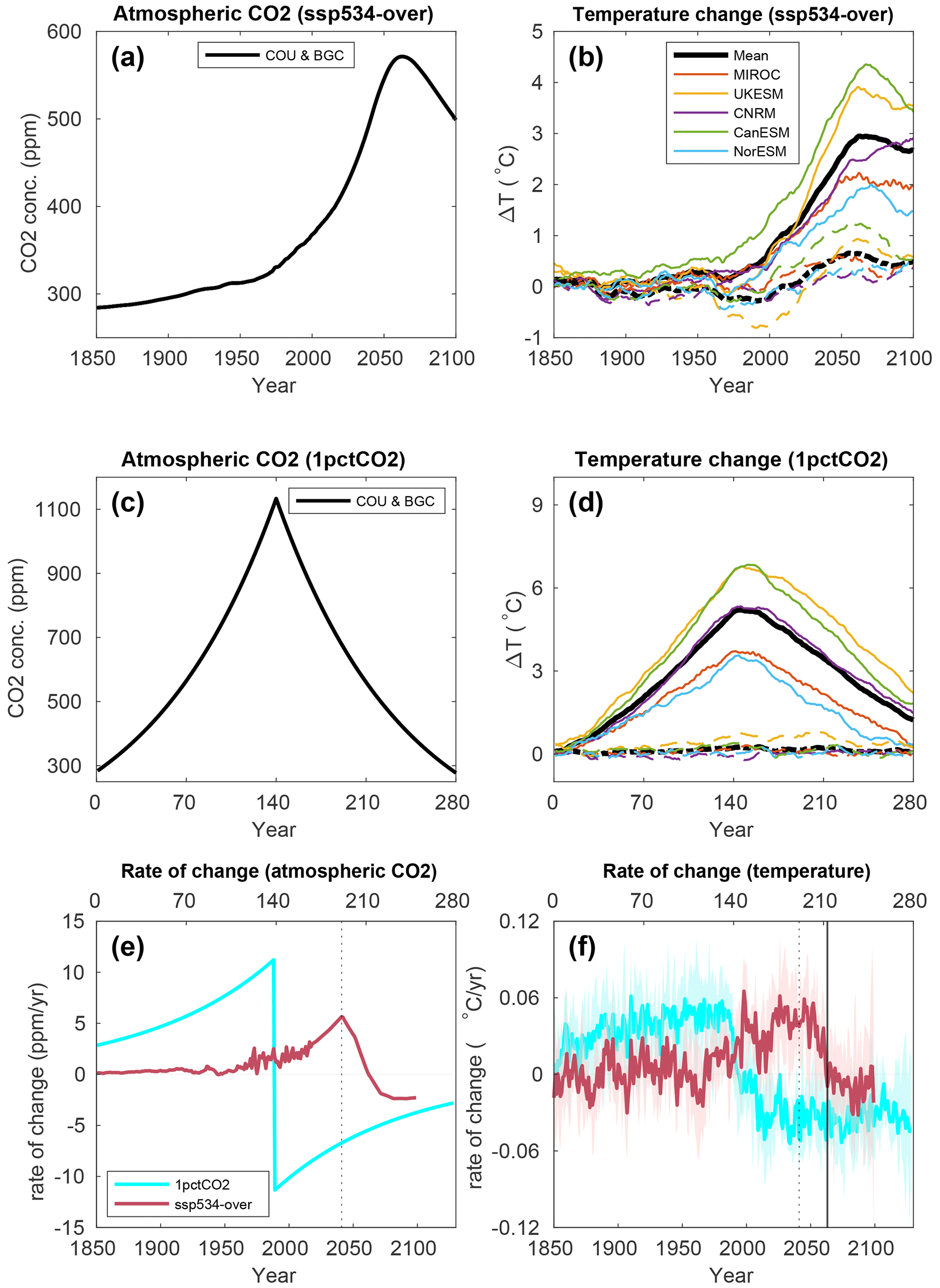
Figure 1 Atmospheric CO₂ concentration and surface air temperature changes in the fully coupled (solid lines) and biogeochemically coupled (dashed lines) configurations of the ssp534-over (a, b) and 1pctCO2-cdr (c, d) experiments. The rates of change in the prescribed atmospheric CO₂ concentrations are shown in (e), and the model mean rate of surface temperature change from the fully coupled simulations is shown in (f). The dotted vertical lines in (e) and (f) indicate the year of the peak of the CO₂ growth rate in the ssp534-over scenario. The solid vertical line in (f) indicates the year of the peak of the CO₂ concentration in the ssp534-over scenario. An 11-year moving average has been used in (b, d, f).

In the 1pctCO2-cdr simulation, the peak temperature anomalies vary from 3.57 ^∘C (in year 144) in NorESM2-LM to 6.84 ^∘C (in year 151) in CanESM5 (Fig. 1d). Thereafter, temperature anomalies decline to values ranging from 0.29 ^∘C in NorESM2-LM to 2.2 ^∘C in UKESM1-0-LL at the end of the ramp-down period (year 280). The 1pctCO2-cdr BGC simulation shows, compared to the ssp534-over BGC simulation, smaller temperature anomalies ranging from −0.22 ^∘C (CNRM-ESM2-1 in year 149) to 0.79 ^∘C (UKESM1-0-LL in year 207). The relatively large magnitude of the temperature anomaly in the ssp534-over-bgc simulation (peak warming of 12 %–29 % of the peak warming in the fully coupled simulation) suggests that warming due to non-CO₂ forcings might contribute substantially to the carbon–climate feedback in the ssp534-over scenario.

For atmosphere–land fluxes, our analysis is complicated by the fact that land-use changes are present in the ssp534-over scenario. Here, we focus on comparing fluxes and feedbacks for grid cells that are dominated by “natural land” (see Sect. 2.2 for more details). Note that, for comparability, we consider the same set of grid cells in the 1pctCO2-cdr simulation, even though land cover stays at its pre-industrial state in this simulation. In the ssp534-over simulations, the model-mean annual CO₂ fluxes (Fig. 2) continue rising until the rate of change in [CO₂] reaches its peak in 2041. After the peak, atmosphere–land and atmosphere–ocean fluxes start to decline rapidly in all models with little time lag. UKESM1-0-LL and MIROC-ES2L simulate negative fluxes (i.e., natural land turns into a carbon source) before the end of the 21st century in the COU simulation (Fig. 2a). Without the effect of CO₂-induced warming (BGC simulation, Fig. 2b), only MIROC-ES2L shows a significant carbon source from the terrestrial biosphere before 2100, while the model-mean still shows a sink. In the fully coupled 1pctCO2-cdr experiment, the sink-to-source transition of the terrestrial biosphere occurs around year 165 in the model mean, 25 years after the rate of change in [CO₂] peaks (Fig. 2c). Consistent with what is seen in the biogeochemically coupled ssp534-over, the sink-to-source transition occurs 10 years later without the effect of warming in the 1pctCO2-cdr-bgc experiment. However, the terrestrial CO₂ source at the end of the biogeochemically coupled 1pctCO2-cdr simulation is larger than in the fully coupled simulation. We also observe that models which take up more (less) terrestrial carbon during the CO₂ ramp-up phase release more (less) carbon towards the end of the CO₂ ramp-down phase (1pctCO2-cdr-bgc; Fig. 2c, d), indicating that these models have a larger (smaller) sensitivity ($\mathrm{\Delta }{\mathrm{C}}_{\text{L}}/\mathrm{\Delta }$CO₂) to both increases and decreases in atmospheric CO₂. We therefore interpret the increased source of carbon at the end of the 1pctCO2-bgc simulation as a release of additional carbon that has been taken up in the absence of climate warming during the biogeochemically coupled simulation. The net negative emission phase of the ssp534-over scenario is too short to show this effect in 2100 (when the warming effect still reduces the model mean terrestrial carbon sink).

Likewise, the warming of the world's oceans in both simulations tends to reduce the carbon uptake or increase the oceanic carbon source. The model spread for atmosphere–ocean carbon fluxes (Fig. 2e–h) appears to be much smaller than for the atmosphere–land fluxes. In the ssp534-over simulation, the ocean remains a sink of carbon in all models until the end of the simulation in 2100. In the 1pctCO2-cdr simulation, the ocean turns into a source of CO₂ for the atmosphere around year 175, and this transition is delayed by 7 years in the BGC simulation without warming.

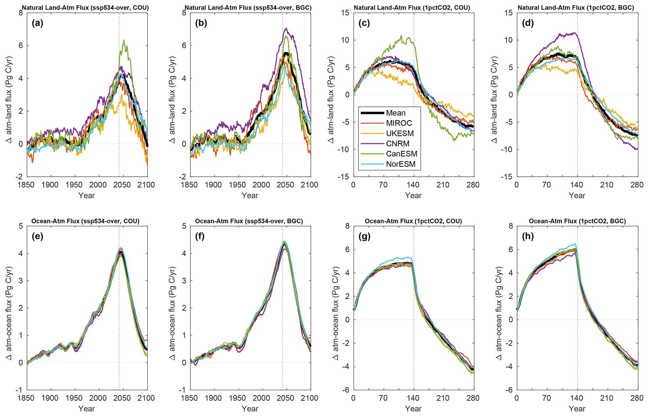
Figure 2 Time series of annual mean natural atmosphere–land (a–d) and atmosphere–ocean (e–h) carbon fluxes for the fully and biogeochemically coupled ssp534-over and 1pctCO2-cdr experiments as indicated in the panel titles. The dotted vertical lines indicate where the [CO₂] growth rate peaks in each experiment. An 11-year moving average has been used in all panels.

3.2 Global mean carbon cycle feedbacks

3.2.1 Ocean

In the BGC simulation, where the effect of the changing atmospheric CO₂ concentration on terrestrial and marine carbon uptake (the carbon–concentration feedback) is isolated, cumulative atmosphere–ocean carbon fluxes indicate an almost linear growth with [CO₂] as long as atmospheric CO₂ concentrations are increasing in both ssp534-over and 1pctCO2-cdr simulations (Fig. 3a–c). When [CO₂] starts to decline, the atmosphere–ocean carbon flux in the 1pctCO2-cdr simulation shows pronounced hysteresis with a continued ocean carbon uptake (until the [CO₂] anomaly has been reduced to roughly 500 ppm) before it starts to decrease towards the end of the ramp-down phase (Fig. 3b). In the ssp534-over-bgc simulation, where the onset of net negative emissions is more gradual, the relationship between cumulative atmosphere–ocean fluxes and [CO₂] during the phase of declining atmospheric CO₂ concentration also shows hysteresis; however, due to the relatively short period of net-negative emissions, the ocean remains a sink of carbon in all models until the end of the simulation.

Differences in the cumulative atmosphere–ocean CO₂ flux between the COU and the BGC simulations versus surface temperature changes (carbon–climate feedback) are shown in Fig. 3d–f. Increasing the temperature results in less carbon uptake by the ocean, except for CNRM-ESM2-1, which simulates slightly more uptake in the first half of the warming period under ssp534-over. During the negative emission phases of the simulations when the air surface temperature is decreasing, the carbon–climate feedback still decreases the ocean carbon content, albeit at reduced rates. Even when pre-industrial CO₂ concentrations are restored at the end of the 1pctCO2-cdr simulation, all models agree that the ocean is still losing carbon due to the effect of (legacy) warming (Fig. 3e). The use of the global average ocean potential temperature (averaged over the full ocean depth) instead of the surface air temperature as a proxy for oceanic climate change, as proposed by Schwinger and Tjiputra (2018), gives a much more linear relationship between changes in the ocean carbon stock and changes in temperature in the majority of the models (Fig. 3g–i). At the end of the ssp534-over and 1pctCO2-cdr simulations, the ocean still holds a large part of the carbon taken up from the atmosphere since pre-industrial times, between roughly 300–400 PgC in 1pctCO2-cdr and around 350 PgC in ssp534-over (Fig. S2).

Generally, the ocean carbon–concentration feedback (as indicated by the cumulative carbon uptake per unit increase of CO₂ concentration, Fig. 3a–c) is larger in the ssp534-over scenario, which can most likely be explained by the slower growth rate of [CO₂] in this scenario compared to the 1pctCO2-cdr simulation (Fig. 3c). For slower growth rates, the ocean has more time to mix and partly transport the adsorbed anthropogenic carbon away from the ocean surface to the interior, increasing the capacity for more uptake. A larger carbon uptake at slower CO₂ growth rates has already been reported by Gregory et al. (2009) and Hajima et al. (2014), although only for combined land and ocean fluxes or land fluxes only. The ocean carbon–climate feedback, in contrast, is slightly smaller in the ssp534-over scenario, i.e., the carbon loss for a given warming is smaller.

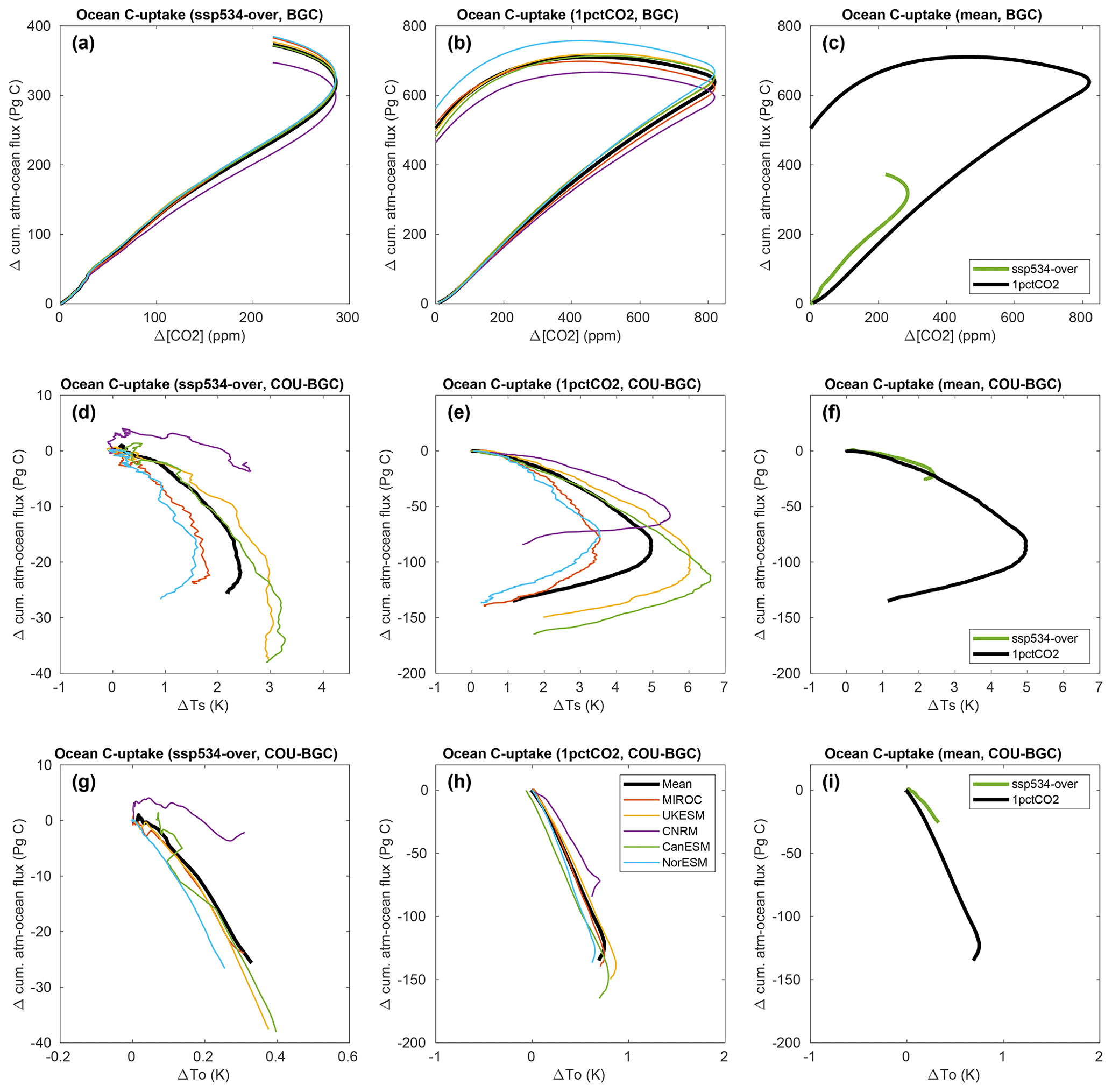
Figure 3 Ocean carbon cycle feedbacks in the ssp534-over (a, d, g) and 1pctCO2-cdr (b, e, h) simulations for individual models. The model means for both simulations are shown in (c, f, i). The global mean ocean potential temperature is used on the x axes of (g–i). An 11-year moving average has been used in all panels.

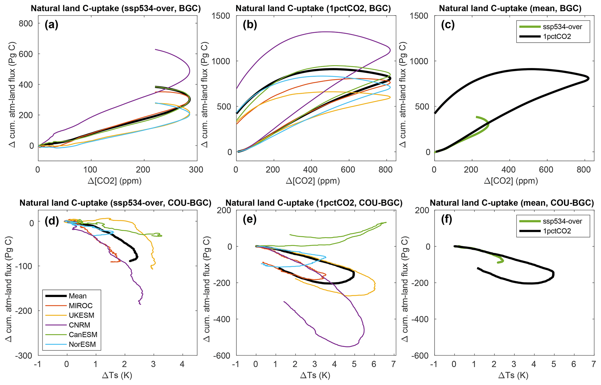
Figure 4 Terrestrial carbon cycle feedbacks in the ssp534-over (a, d) and 1pctCO2-cdr (b, e) simulations for grid cells that are dominated by “natural land” (less than a maximum crop fraction of 25 % over the period 2015–2100 in ssp534-over). Note that we consider the same grid cells in the 1pctCO2-cdr simulation, even though land use stays at the pre-industrial state. The model means for both simulations are shown in (c, f). An 11-year moving average has been used in all panels.

3.2.2 Land

For grid cells representing natural land, the response of the cumulative terrestrial carbon flux to changes in [CO₂] and surface temperature (Fig. 4) is qualitatively similar to the response of the atmosphere–ocean fluxes. In both ssp534-over and 1pctCO2-cdr simulations, a roughly linear relationship can be seen between the carbon flux change and the changes in both [CO₂] and surface air temperature during positive emission phases. An exception is the carbon–climate feedback of the CanESM5 model, which is about zero up to 4^∘ of warming and becomes positive for higher temperature increases. This unique behavior is caused by CanESM5's high climate sensitivity combined with a larger carbon use efficiency amongst CMIP6 models (as shown later), which causes high-latitude vegetation to take up large amounts of carbon in response to warming. This more than compensates for the carbon loss elsewhere that is associated with climate warming. During negative emission phases, both feedbacks show considerable hysteretic behavior, just as for the ocean (see also below). It is worth mentioning that, unlike for the ocean, the COU-BGC accumulated atmosphere–land flux starts to increase, albeit with a lag, in response to cooling during the negative emissions phase in most models (Figs. 3e and 4e).

The carbon–concentration feedback (as indicated by the cumulative carbon uptake per unit increase of CO₂ concentration) is slightly smaller for the ssp534-over scenario compared to the 1pctCO2-cdr experiment (see Fig. 4c), but this difference might be attributed to the remaining influence of land-use changes. This is because, for “cropland grid cells” (with a maximum crop fraction of more than 25 % in the ssp534-over scenario), the cumulative carbon fluxes are markedly smaller in the ssp534-over scenario compared to the 1pctCO2-cdr simulation (compare panel c in Fig. S3 to panel c in Fig. 4). This indicates that the prescribed land-use change in the SSP scenario is the driver behind the small (negative for NorESM2-LM and UKESM1-0-LL) carbon accumulation for cropland grid cells, which is consistent with Melnikova et al. (2022), who demonstrate that carbon losses from land-use changes dominate over gains through CO₂ fertilization in crop-dominated areas (see their Fig. 4a, c). Since grid cells that are dominated by natural land may contain up to 25 % croplands in our separation approach, we expect a reduction in cumulative carbon fluxes due to the remaining land use (changes) in the natural land grid cells. We note that land-use change is externally prescribed rather than a feedback process in our simulations. It is only due to the simulation design used here (see Sect. 2.2 for details) that the carbon release (or uptake) due to land-use change modifies the net atmosphere–land CO₂ flux, which is then seen as a carbon–concentration feedback in the ssp534-over-bgc simulation.

The model-mean carbon–climate feedback for natural land is very similar for the ssp534-over and 1pctCO2-cdr simulations during the positive emission phases but deviates thereafter due to hysteresis behavior (Fig. 4f). Interestingly, in contrast to the carbon–concentration feedback, the model-mean carbon–climate feedback for cropland and natural land remains very similar for the ssp534-over and 1pctCO2-cdr simulations (Fig. S3f). This is likely due to the similar response of the soil carbon to changes in surface air temperature.

3.2.3 Hysteresis

For the 1pctCO2-cdr simulation, hysteresis can be defined as the difference in, for example, cumulative carbon uptake during the ramp-up and the ramp-down periods at the same level of atmospheric CO₂ concentration. Here, to quantify the hysteresis, we choose the years 70 and 210, which represent states where the atmospheric CO₂ has doubled to 570 ppm and has returned to this value after the overshoot, respectively. We define hysteresis as the cumulative carbon uptake in year 210 minus the cumulative carbon uptake in year 70 (i.e., the hysteresis is positive if the cumulative carbon uptake is larger on the ramp-down side of the 1pctCO2-cdr simulation). We refrain from quantifying the hysteresis for the ssp534-over scenario because of the relatively short period of declining [CO₂].

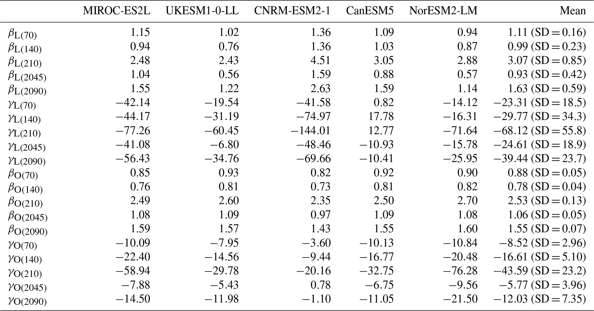
The model-mean hysteresis in the carbon–concentration feedback is 443±29 PgC (the model uncertainty measured as one standard deviation) for the ocean and 524±205 PgC for natural land, which are both larger than the feedback at year 70 itself. Although the hysteresis of the ocean carbon–concentration feedback is smaller than the terrestrial feedback in absolute terms, it is larger in relative terms (179 % of the accumulated carbon uptake at year 70 for the ocean versus 168 % for the land). In general, the hysteresis seems to be related to the magnitude of the carbon–concentration feedback, since models with a large (small) carbon uptake at year 140 tend to show a large (small) hysteresis at year 210 for both ocean and land. However, towards the end of the ramp-down period, this relationship breaks down for CanESM5 and MIROC-ES2L, particularly over land.

For the carbon–climate feedback, the hysteresis in climate-induced carbon loss or gain (the difference between COU-BGC evaluated at year 70 and COU-BGC evaluated at year 210) is $-\mathrm{102}\pm \mathrm{22}$ and $-\mathrm{158}\pm \mathrm{181}$ PgC for ocean and natural land, respectively. Just as for the carbon–concentration effect, a relationship between the magnitude of carbon loss or gain at year 140 and the hysteresis is found. Models with a large (small) climate-induced loss of carbon tend to have a large (small) hysteresis.

For the ocean carbon cycle, hysteresis in the carbon–concentration feedback occurs mainly due to the long timescales of ocean overturning circulations. Schwinger and Tjiputra (2018) have shown that the hysteresis strongly increases with water mass age. Young waters, which reside close to the ocean surface, exchange quickly with the atmosphere and show little hysteresis, whereas the responses of old, deep ocean water masses to declining atmospheric CO₂ will be delayed and thus show considerable hysteresis. Over land, both the vegetation and soil carbon pools show a lagged response to decreasing CO₂ due to the fact that transient changes in [CO₂] lead to a long-term disequilibrium between the CO₂ fertilization effect, vegetation biomass, litterfall, and soil carbon (e.g., Krause et al., 2020). Therefore, despite declining [CO₂] levels at the beginning of the ramp-down phase, there is still an increase in vegetation biomass due to CO₂ fertilization and consequently an increase in soil carbon due to the still-increasing litterfall. Warming-induced hysteresis appears to be larger for soil carbon in most models. Similar to the large warming-induced hysteresis (e.g., Schwinger and Tjiputra, 2018; Schwinger et al., 2022; Santana-Falcón et al., 2023) in the ocean, this is caused by the fact that even though warming levels start to decline shortly after the onset of the ramp-down phase, environmental conditions remain warmer than in the pre-industrial period over the whole duration of the ramp-down simulation.

3.3 Carbon cycle feedback metrics

3.3.1 Model-mean global land and ocean responses

We now discuss the model-mean time evolutions of the feedback metrics β and γ (Eqs. 1 and 2) derived from the 1pctCO2-cdr and ssp534-over simulations. In the ssp534-over scenario (Fig. 5a), the model-mean feedback metric β_L increases monotonically from about 0.7 to 1.9 PgC ppm⁻¹ during the period 2000–2100. Over the ocean, β_O in the ssp534-over scenario decreases slightly until the mid-21st century and then rises to about 1.7 PgC ppm⁻¹. Due to the much larger spread in carbon fluxes over land (Fig. 2), the resulting model spreads for β_L and γ_L are also much larger than those for β_O and γ_O, respectively.

For the 1pctCO2-cdr simulation, β initially increases and then decreases slightly with increasing [CO₂] during the ramp-up phase over both land and ocean (Fig. 5b), consistent with the results of Arora et al. (2013) for the same experiment but using CMIP5 ESMs. In contrast, during the ramp-down phase of the 1pctCO2-cdr experiment, β reaches very high values over both land and ocean (Fig. 5c). This is because, during the carbon removal phase of the 1pctCO2-cdr experiment, there is a much larger amount of accumulated ocean and terrestrial carbon for the same atmospheric CO₂ concentration due to the large hysteresis seen in Figs. 3 and 4. Eventually, while [CO₂] approaches pre-industrial values (i.e., Δ[CO₂] reaches zero), changes in cumulative fluxes (i.e., carbon stocks) relative to their pre-industrial values remain positive, making β ill-defined towards the end of the 1pctCO2-cdr ramp-down. For the same reason, increases in β_L and β_O are also seen in the ssp534-over scenario after the CO₂ concentration peak in 2062.

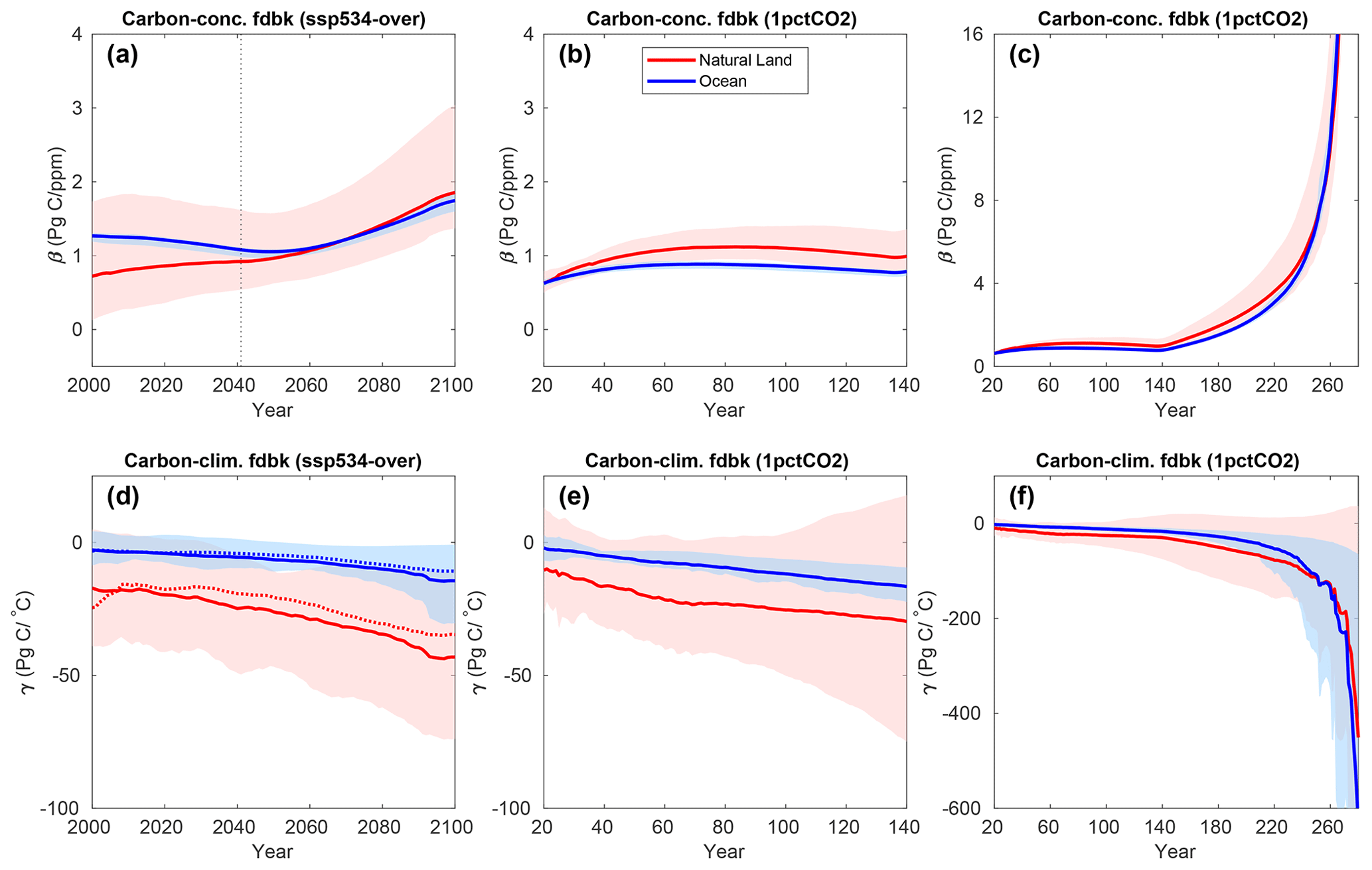
Figure 5 Model-mean feedback metrics β (a–c) and γ (d–f) in the ssp534-over and 1pctCO2-cdr experiments for natural land and ocean. Panels (b) and (e) show zooms of the ramp-up phases of the time series shown in (c) and (f), respectively. Shading shows the range across the models. The dotted vertical line in (a) indicates where the [CO₂] growth rate peaks in the fully coupled ssp534-over experiment. The dotted curves in (d) indicate the model means obtained with the assumption of negligible temperature changes in the BGC simulation (Eq. 2). An 11-year moving average has been used in all panels.

The model-mean feedback factor γ is negative, as the impact of climate change generally reduces the carbon stocks of the land and the ocean. In both the ssp534-over and 1pctCO2-cdr experiments, the carbon–climate feedback increases over time (γ becomes more negative; Fig. 5d and e), similar to Fig. 6 of Arora et al. (2013). The carbon–climate feedback is generally much smaller for the ocean than for land, and the model uncertainty for γ_O is only a small fraction of γ_L. Note that the same globally averaged surface air temperature anomaly is used for the calculation of both γ_O and γ_L (Eq. 2). As noted above, the CanESM5 model simulates a globally increasing land uptake due to climate change towards the end of the 1pctCO2-cdr simulation (Fig. 4e), resulting in a positive γ_L for this model. During the ramp-down phase of the 1pctCO2-cdr experiment (Fig. 5f), γ reaches very large negative values. Similar to β, this is caused by the large hysteresis of the climate change impact on the cumulative carbon stock while the surface temperature change becomes small (see Eq. 2). The assumption of ΔT^BGC=0 generally works well except for γ_L in the ssp534-over scenario, where non-CO₂ forcings make a significant contribution to ΔT^BGC (dashed curves in Fig. 5d).

The global feedback factors B and Γ for the ssp534-over and 1pctCO2-cdr simulations are shown in Fig. S4. These feedback metrics directly reflect the instantaneous fluxes, not cumulative fluxes, and are therefore less influenced by the history of carbon fluxes, unlike β and γ. Consistent with Fig. 2, the model-mean B remains positive during the ssp534-over simulation and during the positive emission phase of 1pctCO2-cdr over both natural land and ocean. Only one model indicates a negative carbon–concentration feedback over natural land towards the very end of the ssp534-over simulation during its relatively short negative emission phase. B reflects the saturation of carbon sinks in the 1pctCO2-cdr simulation with time and decreases monotonically during the positive emission phase. Similar to what we saw earlier for β, B shows large but negative values towards the end of the 1pctCO2-cdr ramp-down phase (Fig. S4c).

An interesting difference between the γ and Γ feedback metrics is seen towards the end of the 1pctCO2-cdr negative emissions phase (Fig. S4f), where Γ_L turns positive around year 180. This indicates that the land biosphere starts gaining carbon that was previously lost due to the impacts of climate change. In contrast, Γ_O remains negative, indicating that the ocean continues to lose carbon due to warmer than pre-industrial conditions until the end of the 1pctCO2-cdr ramp-down phase. Because they are based on cumulative emissions, both γ_O and γ_L remain negative throughout the 1pctCO2-cdr ramp down. This illustrates that the use of a feedback metric based on time-integrated carbon fluxes might obscure changes in important processes during net-negative emission phases. Eventually, both approaches for calculating feedback metrics become ill defined when the deviation of [CO₂] or temperature from its pre-industrial value becomes small. This implies that neither feedback metric is suited to describing feedbacks towards the end (and beginning) of a concentration-driven simulation setup where pre-industrial concentrations are restored. We note that this problem is connected to the choice of the reference relative to which the feedbacks are calculated. In the approach of Chimuka et al. (2023), where the reference is chosen to be at the transition from positive to negative emissions, singularities towards the end of the 1pctCO2-cdr simulation are avoided.

3.3.2 Model uncertainties and relative feedback strength in global feedback metrics

Figure 6 shows the model spread of feedback metrics at different points in time for the 1pctCO2-cdr simulation and the ssp534-over scenario (see also Table 2). The larger model-mean values during the negative emission phases were discussed in the previous section, but Fig. 6 also shows a strong increase in model uncertainty (measured as the standard deviation around the model mean; Table 2) between the ramp-up and ramp-down phases of the 1pctCO2-cdr simulation. For both β_L and β_O, there is either no (β_O) or only a small (β_L) increase in model uncertainty between the years 70 and 140 of the 1pctCO2-cdr simulation, whereas the uncertainty has increased by a factor of about 4 at year 210. This “jump” in uncertainty in β is solely caused by differences in how the models react to the sharp change in forcing from increasing to decreasing CO₂ at year 140 (see Eq. 1; note that atmospheric CO₂ is prescribed and ΔT^BGC is small). Similar behavior is seen for γ_O, while the increase in model uncertainty is more gradual for γ_L, i.e., the increase between years 70 and 140 is about the same as between years 140 and 210. There is also a consistent increase in model uncertainty in all feedback metrics from the positive to the negative emissions phase in the ssp534-over scenario.

The relative feedback strengths among the models remain relatively stable over time, between positive and negative emission phases, and between the different experiments. Model A having stronger (weaker) feedback than model B at one of the instances depicted in Fig. 6 indicates that model A will have stronger (weaker) feedback than model B for the other instances with only a few exceptions. Most of these exceptions arise because modeled feedbacks are very similar, meaning that small changes in feedback strength can lead to a different ranking. In a few cases, the relative feedback strength evolves differently in different models. For example, NorESM2-LM evolves from having a weaker than average γ_L in the positive emission phase of the 1pctCO2-cdr simulation to having a stronger than average γ_L in the negative emission phase.

Finally, it is worth noting that while the model uncertainty in γ_O is much smaller than that in γ_L during the ramp-up phase of the 1pctCO2-cdr simulation (the uncertainty in γ_O is only 15 % of that in γ_L at year 140), this situation changes for the ramp-down phase. At year 210, the uncertainty in the ocean carbon–climate feedback has grown much stronger than the uncertainties in the terrestrial carbon–climate feedback, such that the model uncertainties in γ_O are 42 % of those in γ_L.

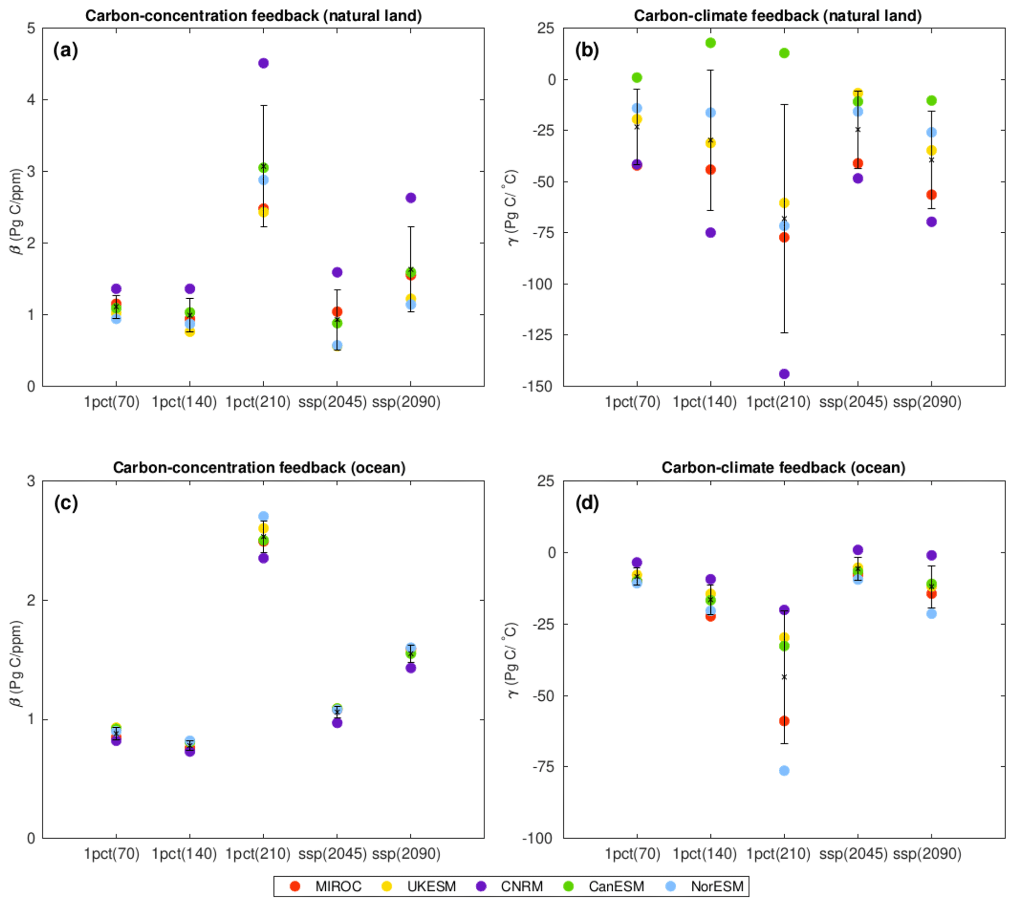
Figure 6 Globally averaged values of β (a, c) and γ (b, d) in the 1pctCO2-cdr (years 70, 140, and 210) and ssp534-over (years 2045 and 2090) experiments for natural land and ocean. The bars show the mean ±1 standard deviation range, and the colored dots represent individual models.

Table 2 Globally averaged values of β (Pg C pm⁻¹) and γ (PgC ^∘C⁻¹) at years 70, 140, and 210 of the 1pctCO2-cdr simulation and years 2045 and 2090 of the ssp534-over experiment for natural land and ocean.

3.3.3 Model differences in the terrestrial carbon–concentration feedback

Figure 7 shows the individual components of the decomposition of β (Eq. 4) separately for tropical and subtropical (30^∘ S–30^∘ N) and higher (between 30^∘ N/S and the poles) latitudes during both the ramp-up and ramp-down phases (years 70 and 210, respectively) of the 1pctCO2-cdr-bgc experiment. The time periods are selected such that the atmospheric CO₂ concentration is the same (569 ppm, a doubling of the pre-industrial CO₂ concentration). All models consistently show increases in both τ_cvegΔ and τ_csoilΔ during the ramp-down compared to the ramp-up phase since these metrics are based on cumulative vegetation and soil carbon (Eq. 4), which are slower than the NPP and GPP in reacting to decreasing [CO₂]. Lower (higher) latitudes are associated with higher τ_cvegΔ (τ_csoilΔ) values. Likewise, the litterfall term $\frac{\mathrm{\Delta }\text{LF}}{\left[{\mathrm{CO}}_{\mathrm{2}}\right]}$ is larger during the ramp-down phase in all models due to the lagged reaction of vegetation carbon to the decrease in [CO₂], with this effect generally being most pronounced at low latitudes. There is also a consistent but small increase in the term $\frac{\mathrm{\Delta }\text{GPP}}{\left[{\mathrm{CO}}_{\mathrm{2}}\right]}$, which represents the CO₂ fertilization effect. This increase implicitly includes the effect of changes (typically an increase) in standing vegetation biomass and leaf area index for all models, but it also includes changes in vegetation cover as [CO₂] varies for UKESM1-0-LL, which simulates dynamic vegetation cover. For the dimensionless fractions $\frac{\mathrm{\Delta }{R}_{\text{h}}}{\mathrm{\Delta }\text{LF}}$ and CUE_Δ, changes between the ramp-up and ramp-down phases are less consistent between the models. For CUE_Δ, three models show an increase and two models show a decrease, although the changes between the ramp-up and ramp-down phases are generally small. For $\frac{\mathrm{\Delta }{R}_{\text{h}}}{\mathrm{\Delta }\text{LF}}$, changes range from a 115 % increase (CNRM-ESM2-1 at low latitudes) to a small decrease (UKESM1-0-LL). It is worth noting that for four out of six terms in Eq. (4) (τ_cvegΔ, τ_csoilΔ, $\frac{\mathrm{\Delta }{R}_{\text{h}}}{\mathrm{\Delta }\text{LF}}$, and $\frac{\mathrm{\Delta }\text{LF}}{\left[{\mathrm{CO}}_{\mathrm{2}}\right]})$, the model disagreement is significantly larger during the ramp-down phase of the 1pctCO2-cdr simulation, indicating that changes in these processes are responsible for the strong increase in model uncertainty in β_L between the positive and negative emission phases pointed out in the previous section.

The decomposition applied here helps us to understand some of the model differences visible in Fig. 4. As already pointed out in Arora et al. (2020), the high accumulation of terrestrial carbon by the CNRM-ESM2-1 model in the BGC simulation (Fig. 4b) is not caused by a particularly strong CO₂ fertilization effect or CUE_Δ but rather by relatively high values of τ_cvegΔ and τ_csoilΔ, indicating long residence timescales in vegetation and soil. Likewise, CanESM5's higher than average atmosphere–land C flux (Fig. 4b) despite its near-average CO₂ fertilization effect strength and soil and vegetation turnover times is due to its high CO₂ fertilization effect at lower latitudes and also its high CUE_Δ, through which the model converts a much larger fraction of the GPP to NPP. Compared to the other models, CanESM5 also shows the largest relative increase (85 % and 134 % for lower and higher latitudes, respectively) in τ_csoilΔ between years 70 and 210.

3.3.4 Northern Hemisphere high-latitude permafrost and non-permafrost regions

Of the ESMs considered here, only NorESM2-LM has a terrestrial model that vertically resolves soil carbon (CLM5, Lawrence et al., 2019). Since this is a prerequisite for skillfully simulating carbon release during gradual permafrost degradation, we restrict our analysis of high-latitude and permafrost feedbacks to the NorESM2-LM model. If only natural land is considered, the area associated with permafrost and non-permafrost regions north of 45^∘ N is about 14.7 and 17.5×10⁶ km², respectively (the total area is 14.7 and 24.1×10⁶ km²).

The effect of warming on carbon uptake in the high-latitude non-permafrost region is positive (γ>0, increased uptake) in NorESM2-LM in both the ssp534-over and the 1pctCO2-cdr simulation (Fig. 8a–c, blue lines). Within the permafrost region, γ is close to zero for the ssp534-over simulation up to 2100 and the ramp-up phase of the 1pctCO2-cdr simulation (Fig. 8a, b, red line), albeit with a decreasing (more negative) trend. This is due to a balance between vegetation carbon gain and soil carbon losses (Fig. S5). During the ramp-down phase of the 1pctCO2-cdr simulation, permafrost soil carbon losses increase until approximately year 210 of the simulation (Fig. S5). Thereafter, permafrost soil carbon stays roughly constant, with a cumulative loss of about 55 PgC over the simulation. Vegetation carbon over the permafrost region still increases for the first 30 years of the ramp-down phase of the 1pctCO2-cdr simulation, after which it decreases, mainly due to a decreasing temperature (Fig. S5g). The γ value calculated for the permafrost region therefore shows a sharp decrease during the ramp-down period of the 1pctCO2-cdr simulation (Fig. 8c). Eventually, when ΔT approaches small values, γ loses its significance, as seen before for the global feedback factors.

In both the ssp534-over scenario and the 1pctCO2-cdr simulations, β is positive (except initially in the ssp534-over simulation), although the absolute values remain very small. The carbon–concentration feedback is stronger over the non-permafrost area, where both soil and vegetation carbon increase, than over the permafrost area, where soil and vegetation carbon stay almost constant in the BGC simulation (Fig. S5).

NorESM2-LM has the smallest transient climate response (TCR) of the models considered here, and it can be expected that the permafrost carbon–climate feedback estimated here would be larger in a model with higher TCR. Nevertheless, the permafrost carbon loss of 26.9 PgC ^∘C⁻¹ in the year 210 of the simulation contributes 38 % of the total carbon–climate feedback at this point in time in NorESM2-LM.

3.4 Geographical pattern of carbon cycle feedback metrics

We have calculated the feedback factors β and γ at grid scale to assess the spatial patterns of feedbacks over the land and ocean (Figs. 9 and 10). In order to compare positive and negative emission phases, we selected 21-year time intervals centered at years 70 and 210 of the ramp-up and ramp-down phases of the 1pctCO2-cdr simulation at an atmospheric CO₂ concentration of 570 ppm (corresponding to a doubling of the pre-industrial CO₂ concentration). We also selected a 21-year time interval centered at year 2045 (corresponding to a CO₂ concentration of 523 ppm), shortly before the CO₂ peak in the ssp534-over scenario. We also analyzed a 21-year time interval during the net-negative emission phase of the SSP scenario (centered at year 2090), but since the time period of net-negative emissions in the SSP scenario is relatively short, we focus on comparing the feedbacks during the positive and negative emission phases of the 1pctCO2-cdr simulation along with the feedbacks during the positive emission phase of ssp534-over. For completeness, Fig. S6 shows the spatially resolved feedback during the net-negative emission phase of ssp534-over.

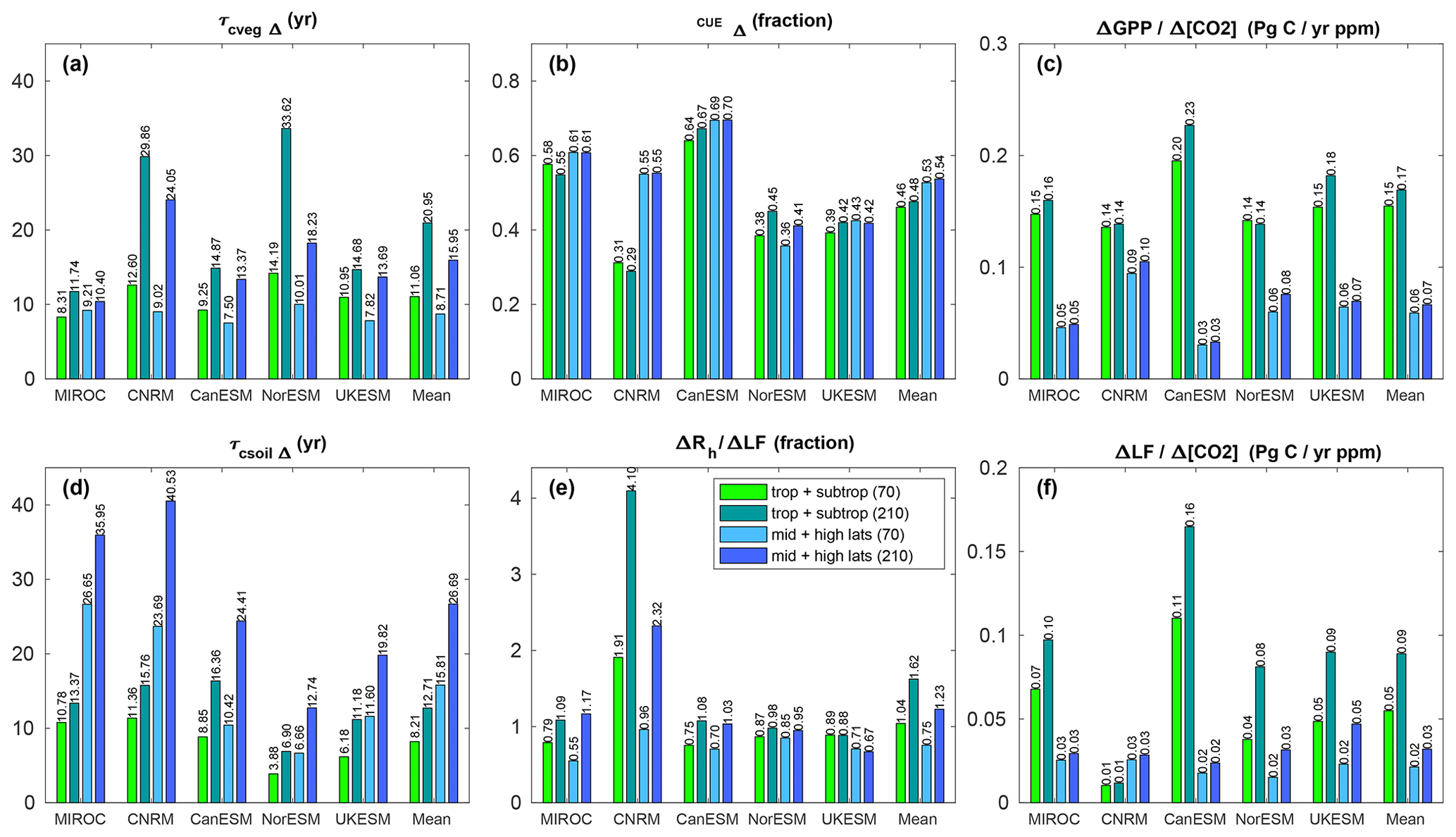
Figure 7 Individual terms in Eq. (4) that contribute to β_L. Values for tropical and subtropical regions (between 30^∘ S and 30^∘ N) are in green, and those for northern and southern latitudes (above 30^∘ S and 30^∘ N) are in blue. Bars with a lighter (darker) color in each panel correspond to the middle of the ramp-up (ramp-down) phase of the 1pctCO2-cdr-bgc experiment (years 70 and 210, respectively).

In the 1pctCO2-cdr simulation, increasing [CO₂] increases the modeled carbon sinks almost everywhere (i.e., positive β) over the land and ocean (Fig. 9a–e). CanESM5 shows a weak negative β over northern high-latitude land areas, and there are some spurious negative values of β over desert areas in some models. For the ocean, all models agree that the regions with the strongest increase in the oceanic CO₂ sinks in response to higher [CO₂] are the North Atlantic and the Southern Ocean. As seen for the global average (Fig. 5), β remains positive and increases in magnitude during the ramp-down phase (Fig. 9f–j; note the different color scales). As an overarching observation, the large-scale patterns of the carbon–concentration feedback are remarkably similar during the ramp-up and ramp-down phases of the 1pctCO2-cdr simulation (with spatial correlations, averaged across all the models, of 0.93 and 0.80 over the land and the ocean, respectively), but the magnitude of the feedback is about two times larger in the ramp-down phase, consistent with the lagged response of cumulative carbon uptake to the decrease in atmospheric CO₂ (Figs. 3 and 4). The most prominent change in the spatial pattern of β occurs in the equatorial Pacific. All models consistently show that this area turns from a cumulative carbon sink at year 70 to a cumulative carbon source at year 210.

We find the largest values of β over tropical land and, to a lesser extent, over Northern Hemisphere temperate and boreal ecosystems coincident with areas of large biomass (forests). For three of the models (NorESM2-LM, CanESM5, and UKESM1-0-LL), the feedback is clearly dominated by tropical and subtropical regions, while for MIROC-ES2L, the feedback is of approximately the same strength in northern temperate and high-latitude regions. For CNRM-ESM2-1, the carbon–concentration feedback is on average stronger north of 30^∘ latitude than it is in tropical/subtropical regions. For NorESM2-LM and UKESM1-0-LL, the tropical dominance of the carbon–concentration feedback stems from vegetation carbon, while for CanESM5, both vegetation and soil carbon contribute about equally (Figs. S7 and S8).

The results presented in Sect. 3.3.3 provide a mechanistic understanding of these model differences to some extent. CNRM-ESM2-1 has the highest CO₂ fertilization effect $\frac{\mathrm{\Delta }\text{GPP}}{\left[{\mathrm{CO}}_{\mathrm{2}}\right]}$ at high latitudes and the lowest CUEΔ at low latitudes. This, combined with a large high-latitude τ_csoilΔ, leads to greater carbon accumulation in vegetation and soil at higher latitudes than in the tropics/subtropics in this model. The three models with a tropical dominance of β (NorESM2-LM, CanESM5, and UKESM1-0-LL) have relatively high τ_cvegΔ and relatively low τ_csoilΔ values. CanESM5 shows the strongest tropical/subtropical CO₂ fertilization effect but also a large response of the litterfall term, leading to large responses in both vegetation and soil carbon.

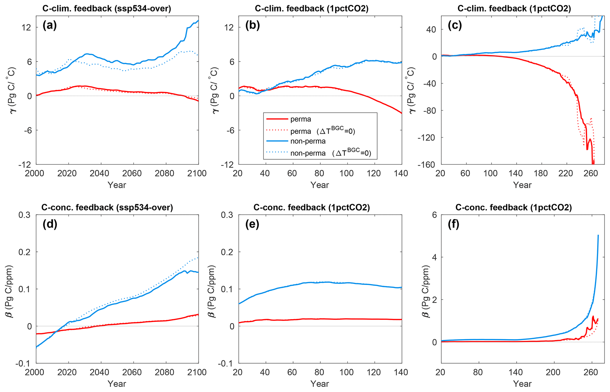
Figure 8 γ (a–c) and β (d–f) for Northern Hemisphere high-latitude (above 45^∘ N) natural land permafrost and non-permafrost regions in the ssp534-over and 1pctCO2-cdr simulations using the NorESM2-LM model. An 11-year moving average has been used in all panels.

In the ssp534-over simulation, the ocean β magnitude is similar to that of the 1pctCO2-cdr simulation, and the spatial distribution of the response of the ocean to the [CO₂] rise is roughly consistent between the models (Fig. 9k–o). In contrast, the feedback pattern over natural land is different in some regions and models between the SSP scenario simulation and the idealized 1pctCO2-cdr experiment. UKESM1-0-LL, CanESM5, and, to a lesser extent, NorESM2-LM project negative β values in some northern high-latitude regions (e.g., Siberia). These negative β values are either not seen at all (UKESM1-0-LL, NorESM2-LM) or are weaker (CanESM5) in the 1pctCO2-cdr simulation, and they originate from a combination of vegetation and soil carbon pools (Figs. S7 and S8). Unlike in the 1pctCO2-cdr experiment, temperature changes are not negligible in the BGC simulation of the ssp534-over experiment (Fig. 1). Furthermore, the spatial pattern of temperature changes is very different for some models, particularly for UKESM1-0-LL, NorESM2-LM, and CNRM-ESM2-1, which show local cooling that is not present (or much weaker) in the fully coupled simulations (Fig. S9). This cooling (and other changes in surface climate related to non-CO₂ forcings) lead to local carbon losses and negative β values in UKESM1-0-LL and NorESM2-LM at northern high latitudes. In addition, according to Eq. (3), these negative values are reinforced by positive β values in this region and a positive global mean temperature change in ssp534-over in these models (see Eq. 3). In contrast, CNRM-ESM2-1 does not show negative values of β at northern high latitudes (despite local cooling), which can be explained by much larger β values to begin with and a smaller (and negative) temperature sensitivity β at high latitudes.

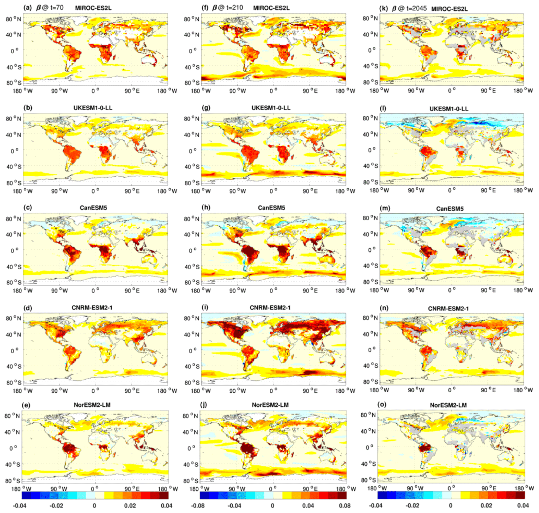
Figure 9 The spatial distribution of β (kg C m⁻² ppm⁻¹) at year 70 of the ramp-up phase of the 1pctCO2-cdr simulation (a–e), at year 210 of the ramp-down phase of the 1pctCO2-cdr simulation (f–j), and at year 2045 (natural land only; gray areas are crop-dominated grid cells) during the positive emission phase of the ssp534-over scenario (k–o).

Figure 10 indicates that the ESMs considered here simulate predominantly negative values of γ_O over the ocean. Positive values of γ_O are found in the Arctic, and most models simulate a banded pattern of positive (adjacent to Antarctica), negative (centered between 60 and 50^∘ S), and positive (between approximately 50 and 40^∘ S) values in the Southern Ocean. In the region adjacent to Antarctica, climate change increases the ocean CO₂ sink, mainly due to a reduction in sea ice coverage (Roy et al., 2011; Schwinger et al., 2014). The North Atlantic Ocean and the Southern Ocean have the largest negative γ_O values due to changes in ocean circulation and deep water formation. In tropical and subtropical ocean regions, the reduced oceanic carbon uptakes can be attributed to warming-induced decreased CO₂ solubility and increased stratification (Roy et al., 2011).

Over land, climate change generally reduces carbon sinks in the tropics and mid-latitudes. In the high latitudes, models disagree on the strength and the sign of the carbon–climate feedback. In northern high latitudes, CNRM-ESM2-1 shows relatively strong soil carbon losses which overcome vegetation carbon gains (Figs. S10 and S11), leading to mostly negative values of γ_L in this region. As mentioned above, CanESM5's carbon–climate feedback switches from weakly negative at 2×CO₂ to positive at 4×CO₂. Figure 10c clearly shows that the positive global γ values originate from the Northern Hemisphere high latitudes. Also, the positive γ_L in CanESM5 over the northern high latitudes is seen in both vegetation and soil carbon reservoirs, but with a time lag for soil carbon. Consistent with our analysis in Sect. 3.3.4, NorESM2-LM shows permafrost carbon loss in northeastern Siberia and northern Alaska, but these losses become significant only during the ramp-down phase of the 1pctCO2-cdr simulation (Fig. 10j).

The spatial pattern of the carbon–climate feedback is similar during the ramp-up and ramp-down phases of the 1pctCO2-cdr simulation, but the magnitude roughly doubles during the ramp-down phase, consistent with the cumulative nature of the γ feedback metric used here (note the different color scales used in Fig. 10). The correlations of the spatial patterns at years 70 and 210 are lower than those for β and range from 0.41 (MIROC-ES2L) to 0.66 (UKESM1-0-LL) for γ_O and from 0.49 (NorESM2-LM) to 0.88 (UKESM1-0-LL) for γ_L.

The value of the feedback metric γ in the ssp534-over scenario simulation is less affected by land-use change, since the same land-use changes are imposed in both the COU and the BGC simulation. In contrast to β, which is directly altered by carbon stock changes due to land-use changes, γ is only influenced indirectly, possibly by different sensitivities of the new vegetation cover after a land-use transition or by changes in local to regional climatic conditions. In terms of the global mean, the carbon–climate feedback during the positive emission phase is very similar for the SSP scenario and the 1pctCO2-cdr simulation (Fig. 5d and e). Also, the spatial patterns of γ_L are largely similar between the ssp534-over and the ramp-up phase of the 1pctCO2-cdr simulation, with correlations ranging from 0.71 (NorESM2-LM) to 0.84 (CNRM-ESM2-1). The largest difference between the two simulations is an enhanced positive feedback over northern high-latitude land in the UKESM1-0-LL model in the SSP scenario compared to the 1pctCO2-cdr simulation, which is seen in both vegetation and soil carbon pools (Figs. S10 and S11). These differences are related to the negative β values (discussed above) for these models, which make the carbon gain due to warming (the difference ΔC^cou−ΔC^bgc) considerably larger than in the 1pctCO2 simulation. Again, this is reinforced by the fact that the global average temperature change in the ssp534-over simulation is positive and thus (ΔT^cou−ΔT^bgc) is smaller than the actual (local) temperature differences. This indicates that, if the global mean temperature change due to non-CO₂ forcings does not broadly reflect local changes correctly (e.g., local cooling vs. global warming), regional-scale feedback factors might show unexpected results.

Over the ocean, the global mean carbon–climate feedback is slightly smaller in ssp534-over compared to the 1pctCO2-cdr simulation (Fig. 3f), but, again, the spatial pattern is largely similar, with correlations ranging from 0.47 (CNRM-ESM2-1) to 0.78 (MIROC-ES2L).

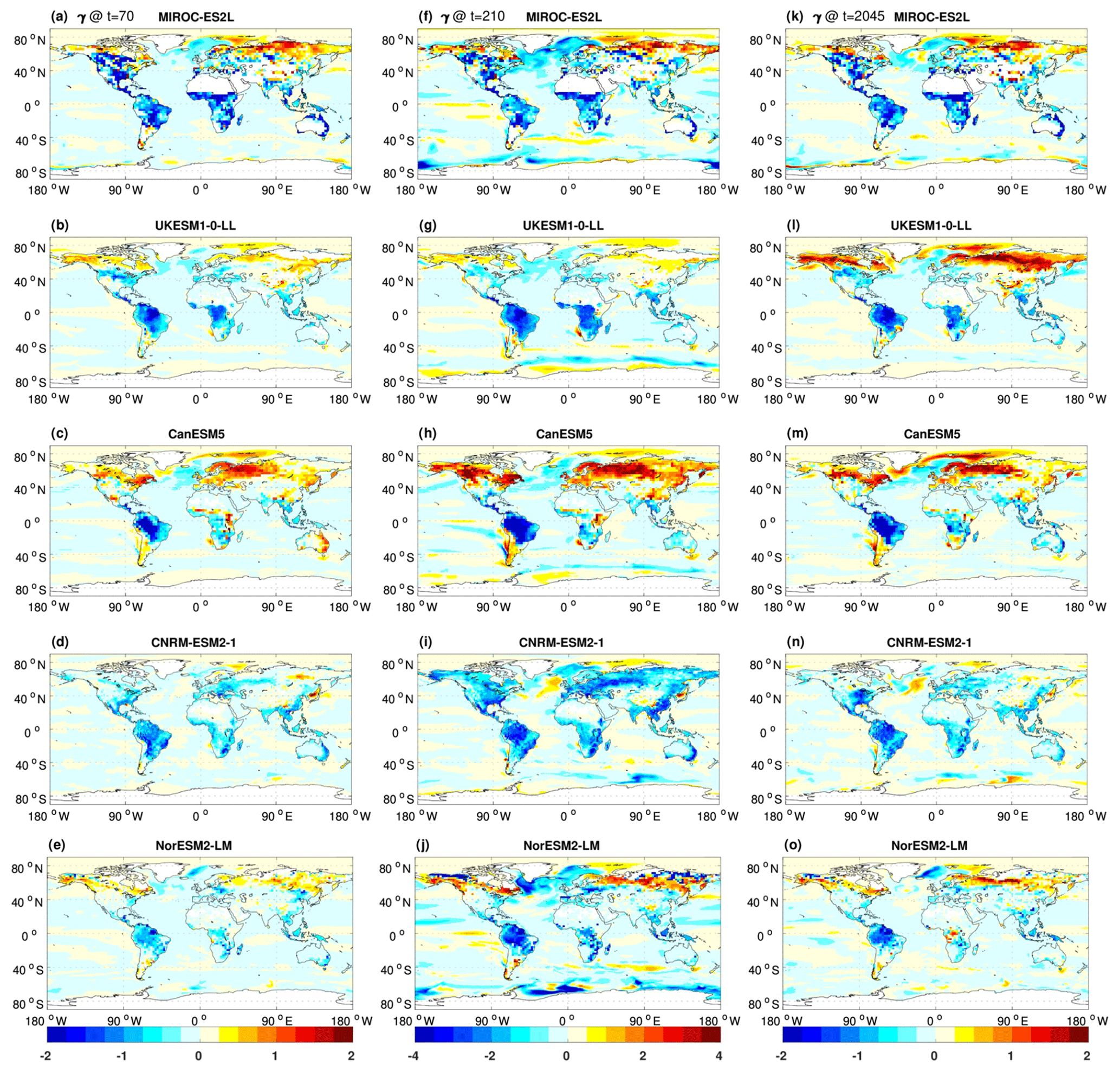
Figure 10 Same as Fig. 9 but for γ (kg C m^−2 ∘C⁻¹). Note that cropland areas are not excluded from panels (k–o) as in Fig. 9.

4 Summary and conclusions

We have investigated carbon cycle feedbacks in a highly idealized model experiment with an exponentially increasing and decreasing atmospheric CO₂ concentration (1pctCO2-cdr) and in a more realistic overshoot scenario simulation (ssp534-over). We employed an ensemble of five CMIP6 ESMs to run additional (biogeochemically coupled) simulations that allowed us to separate out the effects of the changing atmospheric CO₂ and those of the changing surface climate on the simulated carbon cycle.

We find that both the carbon–concentration (β) and the carbon–climate (γ) feedbacks show considerable hysteretic behavior during negative emission phases. The well-known reduction in ocean and land carbon uptake with increasing temperature continues long into the negative emissions phases of the simulations (when the temperature is decreasing), albeit at a reduced rate. For the ocean, there is still a reduction in carbon stocks due to legacy warming when pre-industrial atmospheric CO₂ is restored in the 1pctCO2-cdr simulation, consistent with the single-model studies of Schwinger and Tjiputra (2018) and Bertini and Tjiputra (2022). In contrast, all models agree that the effect of legacy warming is less important for the terrestrial carbon–climate feedback, as reducing the global mean surface temperature leads to a reduction in temperature-induced losses of terrestrial carbon towards the end of the 1pctCO2-cdr simulation.

Carbon cycle feedback metrics vary over time and between different scenarios. When the deviations in surface temperature and atmospheric CO₂ become small towards the end of a modeled negative emission scenario, the magnitudes of these feedback metrics “explode”, since they are defined as the ratio between the deviations in carbon stocks and the change in temperature and atmospheric CO₂, respectively. Arguably, the latter is mainly a problem in the 1pctCO2-cdr experiment due to the strongly idealized simulation design, but not for more realistic scenarios such as ssp534-over. Also, using a different definition of the reference state for the feedback metrics, as proposed by Chimuka et al. (2023), avoids this problem.

We find that the relative strength of the feedback remains relatively robust between positive and negative emission phases and between the different simulations considered here. For example, a model with a stronger than average terrestrial carbon–concentration feedback (β_L) during the positive emission phase of the 1pctCO2-cdr simulation will also show a stronger than average β_L during the negative emission phase or for the ssp534-over scenario. Regarding the model uncertainty in feedback metrics, we find that there is an increase in uncertainty in all feedback metrics between the positive and negative emission phases of the 1pctCO2-cdr simulation. Except for γ_L, this increase is much larger than expected from an accumulation of uncertainty over time. This indicates that there is an additional component of model uncertainty resulting from differences in the lagged model responses to the change from increasing to decreasing radiative forcing.

The geographical patterns of the terrestrial feedback metrics β and γ highlight that differences in the responses of tropical/subtropical versus temperate/boreal ecosystems are a major source of model disagreement. For individual models, however, the spatial feedback patterns are remarkably similar during phases of increasing CO₂ compared to phases of decreasing CO₂ concentrations, indicating that the increases in the global mean values of β and γ due to lagged responses of the carbon cycle during negative emissions phases do not stem from a particular region but are generally seen over the whole globe. We only estimated the contribution of permafrost carbon release to the carbon–climate feedback for one of the five ESMs (NorESM2-LM, which vertically resolves soil carbon). Permafrost carbon release is clearly seen as a strong positive feedback (i.e., negative γ) over the permafrost area, but it emerges relatively late in the simulations. Permafrost carbon release accounts for 38 % of NorEMS2-LM's carbon–climate feedback at the midpoint of the negative emission phase of the 1pctCO2-cdr simulation.

In the ssp534-over simulation, the presence of land-use change complicates the analysis of feedbacks. Land-use change is not a feedback process; yet, owing to the C4MIP simulation design, carbon losses (or gains) due to land-use change are confounded with the carbon–concentration feedback derived from a biogeochemically coupled scenario simulation. If we disregard agricultural areas, terrestrial carbon cycle feedback patterns in the ssp534-over scenario are largely similar to those in the 1pctCO2-cdr simulation, although there are some differences, particularly in high northern latitudes due to the influences of non-CO₂ forcings.

We conclude with some recommendations for future research and the design of future model intercomparison projects (MIPs) like C4MIP and CDRMIP. Attempts to identify and better understand the causes of differences in the lagged model response to decreasing emissions, which we have shown to increase the model disagreement under negative emissions, should be pursued further with high priority. The feedback metrics based on the integrated flux (β and γ) and those based on the instantaneous flux (B and Γ) as well as their uncertainties become difficult to interpret in scenarios where the atmospheric CO₂ concentration decreases, particularly in the extreme case when the atmospheric CO₂ concentration and the surface temperature approach their pre-industrial levels. In the light of the discussion around CDR, perhaps it is time to rethink other related forms of these metrics (e.g., see Chimuka et al., 2023) that describe the response of land and ocean carbon systems in scenarios of decreasing atmospheric CO₂ in a more robust manner.

The 1pctCO2 simulation combined with the 1pctCO2-cdr simulation is an extremely idealized model experiment with huge (and infeasible) amounts of implied net-negative emissions and a discontinuity at year 140, when implied emissions jump from large positive to large negative values. As we know that carbon cycle feedbacks are scenario dependent, it would be preferable to assess these feedbacks using model simulations that have a more realistic emission pathway and that include more realistic amounts of net-negative emissions. Alternative idealized simulation designs that include negative emissions have been proposed in the literature (MacDougall, 2019; Schwinger et al., 2022), and we have also considered the ssp534-over scenario in this study. However, the presence of land-use change and variable non-CO₂ forcings in SSP scenarios complicates the quantification of carbon cycle feedbacks. Whether this problem can be solved for future phases of C4MIP by providing more detailed model output or by requesting additional idealized experiments (e.g., scenario simulations with fixed land use) should be discussed in the C4MIP community.

Finally, most proposed negative emission options would be realized by manipulating the terrestrial or oceanic carbon sinks (e.g., bioenergy with carbon capture and storage, afforestation, or ocean alkalinization), thereby not only changing the atmospheric CO₂ concentration and possibly the surface climate but also the carbon cycle feedbacks themselves. Such interactions go beyond what can be addressed with the traditional C4MIP design of fully and biogeochemically coupled ESM simulations. Consequently, a new framework for determining feedbacks caused by large-scale CDR in realistic scenarios of CDR deployment is needed and should be developed in close collaboration with the integrated assessment modeling community that will create such scenarios.