The effects of land use on soil carbon stocks in the UK

Greenhouse gas stabilisation in the atmosphere is one of the most pressing challenges of this century. Sequestering carbon in the soil by changing land use and management is increasingly proposed as part of climate mitigation strategies, but our understanding of this is limited in quantitative terms. Here we collate a substantial national and regional data set (15 790 soil cores) and analyse it in an advanced statistical modelling framework. This produced new estimates of the effects of land use on soil carbon stock (S_c) in the UK, different in magnitude and ranking order from the previous best estimates. Soil carbon stocks were highest in woodlands, followed by rough grazing, semi-natural grasslands, and improved grasslands, and they were lowest in croplands. Estimates were smaller than the previous estimates, partly because of new data, but mainly because the effect is more reliably characterised using a logarithmic transformation of the data. With the very large data set analysed here, the uncertainty in the differences among land uses was small enough to identify consistent mean effects. However, the variability in these effects was large, and this variability was similar across all surveys. This has important implications for agri-environment schemes seeking to sequester carbon in the soil by altering land use, because the effect of a given intervention is very hard to verify. We examined the validity of the “space-for-time” substitution, and, although the results were not unequivocal, we estimated that the effects are likely to be overestimated by 5 %–33 %, depending upon land use.

1 Introduction

Conversion of land to agricultural use has had a significant impact on the global carbon cycle (Le Quéré et al., 2009; Wilkenskjeld et al., 2014; Obermeier et al., 2021). This is expected to continue with the rising human population and demand for agricultural land in some regions and to move towards reforestation and rewilding in other regions (Gitz and Ciais, 2004; Levy et al., 2004; Lawrence et al., 2016). Different land uses affect the inputs of organic matter to the soil (via plant litter, crop residues, root death, and animal necromass) and affect the losses via heterotrophic respiration and leaching. Depending on how a given land use affects the balance of these gains and losses, the soil carbon stock (S_c) may be increased or decreased, relative to its previous state (Ostle et al., 2009). Under the UNFCCC agreement, each nation is required to estimate its net emission or sequestration of carbon attributable to land-use change, as accounted for under the reporting rules for land use, land-use change, and forestry (LULUCF) (Intergovernmental Panel on Climate Change (IPCC), 2003). The default method involves estimating the difference in the long-term equilibrium soil carbon stock among different land uses. Along with data on the area of land undergoing the transition from each land-use type to every other land-use type (i.e. a matrix of land-use change), this is then used to dynamically model the change in soil carbon for each land-use transition each year. The key parameters in this model are the equilibrium soil carbon stock values for the different land uses. In the UK, these are estimated using a space-for-time substitute approach, based on a nationwide survey of soil carbon stock, stratified by land use and soil series (Milne and Brown, 1997; Bradley et al., 2005). By examining the differences in soil carbon stock among land uses occurring on the same soil series, and averaging across >400 soil series which cover the UK, we can estimate the overall mean effect of each land use on soil carbon stock.

Data from several other soil surveys have become available since 2005, but these differ in their methods, most critically in terms of the soil depth sampled, with many focusing on the more easily sampled top soil. In the absence of measurements over the whole profile, these more recent data have not previously been used to update the estimates of UK soil carbon stocks of Bradley et al. (2005) or the effects of land-use change. However, there are some issues with the approach of Bradley et al. (2005) which make updating these estimates timely. Bulk density was generally estimated using pedotransfer functions, which use organic carbon content as a predictor, and quite how this non-independence may affect the results is unclear. Some of the details of the analysis with respect to land use are not completely clear (the equations used are not available), and different choices and assumptions (about the land-use classification or data transformations, for example) can give quite different results.

A weakness of the general approach is in the assumption that the space-for-time substitution is fully valid: we assume that the spatial differences observed in soil carbon stock within a soil series are completely attributable to differences in land use. This will be inappropriate if there are systematic pre-existing differences in the soil carbon stock on the land chosen for particular uses (such as arable crops, pasture, and forestry). For example, the flat, low-lying, free-draining soils typically chosen for arable crops might differ substantially from the higher-elevation marginal land typically chosen for forestry. If there are such differences, this will confound the analysis, such that we wrongly ascribe cause and effect.

The alternative to the space-for-time substitution approach is to measure the effect of a land-use change at a single site repeatedly over time. However, the number of such studies is very small because of the long timescale required to detect change and the large sample size needed to detect change above the local-scale variability (Schrumpf et al., 2011). Paired-plot or chronosequence studies represent a compromise, whereby the space-for-time substitution assumption is still made but the spatial variability is minimised by choosing closely co-located plots. However, the variability found in such studies is still rather large (Poeplau et al., 2011). Some survey data suggest that the change in soil carbon occurs over time, irrespective of land-use change (Bellamy et al., 2005; Reynolds et al., 2013), though whether changes are real or general or what causes them is subject to debate (Smith et al., 2007; Chamberlain et al., 2010). Although most of the survey data cover only a single short period of time, the Countryside Survey data are repeated measurements within the same 1 km squares since 1978. Although bulk density measurements were missing initially, these can still be used to examine possible trends in time (Thomas et al., 2020a).

The work described here attempted to improve quantification of the effects of land use on soil carbon stocks in the UK by (i) incorporating more recent survey data, (ii) applying more sophisticated statistical modelling, and (iii) rigorously assessing the validity of the assumption behind the space-for-time substitution. As a check for confounding variation, we look for evidence of change over time not caused by land-use change where the data allow this.

1.1 Hierarchical model

Different soil surveys have been carried out for different purposes, using different protocols, and differ in the depth that is sampled. For example, the CEH Countryside Survey (Emmett, 2010) has a large spatial coverage, with repeated sampling at the same locations, but only samples the top 15 cm of soil. Other surveys have sampled down to a depth of 1 m or more, but they have limited coverage of land uses and only occur at one point in time (e.g. Ward et al., 2016). Measurements of bulk density, essential for calculating S_c via Eq. (4), are sometimes missing and may have to be imputed from pedotransfer functions. This creates a problem in that the data from different surveys are not directly comparable and that estimating S_c over the whole profile from the available data is not straightforward (Kravchenko and Robertson, 2011).

Our approach to this is to use a Bayesian hierarchical model to estimate S_c as a function of depth. There are strong theoretical grounds for expecting an exponential decline in soil carbon with depth. Firstly, the biomass of plant roots declines exponentially with depth, and this is a major source of carbon input via exudates and root death. Secondly, plant litter is deposited at the soil surface and moves downwards in a quasi-stochastic manner (via soil macrofauna, disturbance events, and leaching), which will produce an exponentially decreasing vertical distribution. The theory is borne out by empirical data: Jobbágy and Jackson (2000) found a logarithmic relationship between soil carbon stock and depth in a meta-analysis of more than 2700 soil profiles. Soil carbon stock is itself the product of two variables with sizeable sampling error (bulk density and carbon fraction in Eq. 4), so it would be expected to show a lognormal frequency distribution. This is also borne out by the analysis of Jobbágy and Jackson (2000), who found that a logarithmic transformation of carbon stock fitted the key assumptions of linear modelling (normality, homoscedasticity, and linearity) much better, according to various diagnostic criteria.

Clearly, one could model this relationship using ordinary linear regression. However, a Bayesian hierarchical approach has several advantages. Firstly, it allows us to “borrow strength”: by correctly representing the structure of the data, we can incorporate data from sub-populations of similar but distinct groups (e.g. data from different sites, locations, or surveys). In this way, it produces more accurate estimates because it distinguishes between artefacts of the sampling process, rather than assuming all data points are the same and lumping all unexplained variance into a single error term. As such, it can account for the fact that replicate soil cores from the same location at the same site are not independent samples but will tend to be similar because of their co-location (and therefore have similar systematic differences from the global mean). Similarly, it can account for vagaries of different surveys, acknowledging that the errors and biases are likely to be similar in data from the same survey, because of systematic differences in protocols, laboratory procedures, and instrument calibrations. For example, the temperature and duration in the combustion furnace used can have a systematic effect on apparent carbon content measured by loss on ignition (LOI) (Hoogsteen et al., 2015), but such vagaries are not explicit in the data typically available.

Secondly, the Bayesian approach allows us to propagate the uncertainty correctly because we quantify the joint posterior distribution of all the parameters that we estimate (Gelman et al., 2013). Thirdly, it allows us to bring in information from other sources as informative priors. For example, we can use the meta-analysis of Jobbágy and Jackson (2000) to set sensible values and ranges on the prior estimates for the parameters describing the relationship with depth. We can thus develop a statistical model which allows us to incorporate disparate data sets into coherent estimates of whole-profile carbon stock, propagating the associated uncertainty appropriately. Critically, we can make use of the many observations collected at shallow depths, and use these to improve the estimates of whole-profile carbon stock and the effects thereon of land use, whilst representing the uncertainty associated with the fact that these are not measurements of whole-profile carbon stock.

1.2 Validity of space-for-time substitution

We can use a number of approaches to investigate the validity of the assumption behind the space-for-time substitution.

1. We would expect any increases in S_c which are caused by land-use change to be independent of the initial S_c. By contrast, we expect any pre-existing differences within a soil series to be in relative terms: a given soil series might have a high mean S_c, and the differences between land chosen for arable cropping and forestry will be proportional to this. We can therefore examine whether the ostensible effects of land use are consistent with models of absolute or relative change. The degree of relative change can be equated with pre-existing difference, and the confounding effect can be removed from the space-for-time substitution.

2. Along similar lines to the above, we can explore correlations between altitude and S_c, removing the effect of land use. Altitude affects climate and soil formation, and this strongly influences choices made over land use, such that different land uses lie on a gradient: as altitude increases, there is a general shift from arable crops to improved pasture, rough grazing, and forestry. If there are pre-existing differences in S_c along this gradient irrespective of land use, then this can be estimated and the confounding effect can be accounted for.

3. In a Bayesian approach, we can use prior information in combination with observed data to improve our estimates. In the current context, we have information from previous paired-plot studies and modelling studies, which gives us an expectation of the likely magnitude of land-use effects. This can be used to counter-balance artefacts which may exist in the space-for-time survey-based estimates of these effects.

1.3 Aims

Our aims here were to improve the estimates of the effects of land use on soil carbon stocks in the UK by

• using more recent survey data to update the estimates of Bradley et al. (2005);

• developing a Bayesian hierarchical model whereby data from different surveys and sampling depths can be incorporated into estimates of whole-profile carbon stock, propagating the associated uncertainty appropriately; and

• investigating the validity of the assumption behind the space-for-time substitution.

2 Methods

2.1 The measurement of soil carbon stock and notation

Naming of the relevant quantities involved in measuring soil carbon is rather inconsistent, and it is useful to define some notation. Sampling is usually done by extracting a soil core with an auger or, less commonly, by digging a soil pit (see Nayak et al., 2019, for a recent review of field and laboratory methods). This provides a sample with known area (A in m²) which is typically divided into one or more depth intervals. These intervals are defined by upper and lower boundaries z₁ and z₂, with length $d=z_{\mathrm{2}}-z_{\mathrm{1}}$ in metres. The soil from each depth interval is treated as a separate sample for laboratory analysis. The common laboratory process is to sieve the soil through a 2 mm sieve, removing stones, roots, and any identifiable litter or living material to leave the fine earth component (subscript _fe). The total mass of fine earth (M_fe in kg) in each sample is oven-dried, weighed, and expressed per unit volume to give the bulk density:

$$\begin{array}{}\text{(1)}& {\mathit{\rho }}_{\mathrm{fe}}={\displaystyle \frac{M_{\mathrm{fe}}}{\mathrm{d}A}}\left[\mathrm{kg}{\mathrm{m}}^{-\mathrm{3}}\right].\end{array}$$

The organic carbon content of the fine earth is determined on a very small sub-sample, typically less than 10 g when using the loss-on-ignition (LOI) method or <1 g when using the elemental analyser method, so the soil needs to be ground and well mixed to homogenise and replicates need to be taken. In the LOI method, a dried sub-sample is weighed and then heated to around 350–500 °C for several hours (Ball, 1964; Hoogsteen et al., 2015) so that the organic matter is combusted to CO₂ gas and water vapour. The sample is re-weighed, and the mass loss is attributed to organic matter; around 55 % of this is carbon, depending on the chemical composition of the organic matter. In an elemental analyser, the combustion gas is trapped, and the exact amounts of CO₂ and H₂O are determined, so that the carbon loss is measured directly. Often, elemental analysis is used to verify or calibrate the carbon fraction determined by LOI. Depending on the analytical setup, the total (as opposed to only organic) carbon content may be measured, from which the inorganic fraction has to be estimated, and this may be significant in UK soils. The mass of carbon (M_c) is expressed as a fraction of the mass of fine earth to give the carbon fraction (also referred to as carbon content or concentration):

$$\begin{array}{}\text{(2)}& f_{\mathrm{c}}={\displaystyle \frac{M_{\mathrm{c}}}{M_{\mathrm{fe}}}}\left[\mathrm{kg}{\mathrm{kg}}^{-\mathrm{1}}\right].\end{array}$$

The product of this and bulk density gives the density of carbon:

$$\begin{array}{}\text{(3)}& {\mathit{\rho }}_{\mathrm{c}}={\mathit{\rho }}_{\mathrm{fe}}{f}_{\mathrm{c}}\left[\mathrm{kg}{\mathrm{m}}^{-\mathrm{3}}\right].\end{array}$$

The quantity we are ultimately interested in is the mass of carbon per unit ground area, i.e. the areal density, more commonly referred to as the carbon stock. This quantity always has some implicit value of depth associated with it. We may refer to the areal density of fine earth or carbon within a given depth interval i,

$$\begin{array}{}\text{(4)}& {\displaystyle }{s}_{\mathrm{fe},i}=d_i{\mathit{\rho }}_{\mathrm{fe},i}\left[\mathrm{kg}{\mathrm{m}}^{-\mathrm{2}}\right]\text{(5)}& {\displaystyle }{s}_{\mathrm{c},i}=d_i{\mathit{\rho }}_{\mathrm{c},i}\left[\mathrm{kg}{\mathrm{m}}^{-\mathrm{2}}\right],\end{array}$$

and denote this with a lower-case s. We can accumulate these with depth through the soil profile to give the cumulative areal density down to a given depth z,

$$\begin{array}{}\text{(6)}& {\displaystyle }{S}_{\mathrm{fe},z}=\sum _{i=\mathrm{1}}^n{s}_{\mathrm{fe},i}\left[\mathrm{kg}{\mathrm{m}}^{-\mathrm{2}}\right]\text{(7)}& {\displaystyle }{S}_{\mathrm{c},z}=\sum _{i=\mathrm{1}}^n{s}_{\mathrm{c},i}\left[\mathrm{kg}{\mathrm{m}}^{-\mathrm{2}}\right],\end{array}$$

and denote this with an upper-case S; n is the number of intervals above depth z. As discussed below (Sect. 2.2), there are statistical issues in estimating the cumulative quantity in this way.

The areal density S_c may be calculated for a specified depth z or for a specified mass of fine earth M_fe (i.e. spatial or cumulative mass coordinates sensu Gifford and Roderick, 2003; see Ellert and Bettany, 1995). The latter is important for removing confounding effects of changes in bulk density (or sample compression) when only the upper layers of soil are measured, on the assumption that the areal density of fine earth S_fe does not change, even if the bulk density ρ_fe does change (Toriyama et al., 2011). The distinction is less critical if measurements effectively encompass the bulk of the soil profile (down to ∼0.6 to 1 m): if a large majority of the soil containing organic material is sampled, then it matters less whether this is expressed in spatial or cumulative mass coordinates. More critically, we want a method which allows us to combine data from surveys which use different sampling depths, both shallow and deep. We describe this below.

2.2 Model development

Our approach was to build a parsimonious statistical model which explains the variability in the observations of soil carbon as a function of land use and depth. Often the cumulative soil carbon stock S_c,z is used as the response variable, but this violates the assumption of independence among samples. The value of S_c,z at each depth is contingent on all values at shallower depths being correct, so this underestimates the uncertainty. By using the variables that are actually measured, we can more correctly represent the structure of the data and thereby more accurately quantify the associated uncertainty.

For each soil core i from land use u occurring at location j within site k, we predict the carbon density ρ_c as a linear function of the sampling depth z, according to the following:

$$\begin{array}{}\text{(8)}& \begin{array}{rl}{\displaystyle }\log ({\mathit{\rho }}_{c,z,u}{)}_i& {\displaystyle }\sim N\left(\mathit{\mu },{\mathit{\sigma }}^{\mathrm{2}}\right)\\ {\displaystyle }\mathit{\mu }& {\displaystyle }={\mathit{\beta }}_{\mathrm{0},u}+{\mathit{\beta }}_{\mathrm{1},u}z+b_{\mathrm{0}j\left[i\right],k\left[i\right]}+b_{\mathrm{1}j\left[i\right],k\left[i\right]}z\\ {\displaystyle }\\ {\displaystyle }\left(\begin{array}{c}\begin{array}{rl}{\displaystyle }& {\displaystyle }{b}_{\mathrm{0}j}\\ {\displaystyle }& {\displaystyle }{b}_{\mathrm{1}j}\end{array}\end{array}\right)& {\displaystyle }\sim N\left(\left(\begin{array}{c}\begin{array}{rl}{\displaystyle }& {\displaystyle }{\mathit{\mu }}_{b_{\mathrm{0}j}}\\ {\displaystyle }& {\displaystyle }{\mathit{\mu }}_{b_{\mathrm{1}j}}\end{array}\end{array}\right),\left(\begin{array}{cc}{\mathit{\sigma }}_{b_{\mathrm{0}j}}^{\mathrm{2}}& {\mathit{\rho }}_{b_{\mathrm{0}j}{b}_{\mathrm{1}j}}\\ {\mathit{\rho }}_{b_{\mathrm{1}j}{b}_{\mathrm{0}j}}& {\mathit{\sigma }}_{b_{\mathrm{1}j}}^{\mathrm{2}}\end{array}\right)\right),\\ {\displaystyle }& {\displaystyle }\text{for loc\_id:site\_id}j=\mathrm{1},\mathrm{\dots },J\\ {\displaystyle }\\ {\displaystyle }\left(\begin{array}{c}\begin{array}{rl}{\displaystyle }& {\displaystyle }{b}_{\mathrm{0}k}\\ {\displaystyle }& {\displaystyle }{b}_{\mathrm{1}k}\end{array}\end{array}\right)& {\displaystyle }\sim N\left(\left(\begin{array}{c}\begin{array}{rl}{\displaystyle }& {\displaystyle }{\mathit{\mu }}_{b_{\mathrm{0}k}}\\ {\displaystyle }& {\displaystyle }{\mathit{\mu }}_{b_{\mathrm{1}k}}\end{array}\end{array}\right),\left(\begin{array}{cc}{\mathit{\sigma }}_{b_{\mathrm{0}k}}^{\mathrm{2}}& {\mathit{\rho }}_{b_{\mathrm{0}k}{b}_{\mathrm{1}k}}\\ {\mathit{\rho }}_{b_{\mathrm{1}k}{b}_{\mathrm{0}k}}& {\mathit{\sigma }}_{b_{\mathrm{1}k}}^{\mathrm{2}}\end{array}\right)\right),\\ {\displaystyle }& {\displaystyle }\text{for site\_id}k=\mathrm{1},\mathrm{\dots },K.\end{array}\end{array}$$

The β₀ and β₁ parameters represent the global intercept and slope parameters specific to each land use (“fixed effects” in the mixed-modelling jargon). The b₀ and b₁ parameters represent group-specific parameters describing the variability among sites and at locations within sites (“random intercepts and slopes” in the mixed-modelling jargon). These local deviations in intercepts and slopes account for the within-location correlation or site correlation of residuals, and they are assumed to be independently drawn from normal distributions with the means and covariance matrices shown above. Analogous terms can be added to account for systematic differences between surveys (i.e. data sources), but they are not shown here for brevity. The only difference is that these are crossed effects, applying to all sites within a survey, rather than nested effects.

The parameters of hierarchical models are commonly estimated by maximum-likelihood estimation (MLE). Here, we used MLE for exploratory analysis but used a Bayesian method for the final model, for the reasons given earlier. Bayesian methods generally uses Markov chain Monte Carlo (MCMC) sampling, an iterative algorithm for calculating numerical approximations of multi-dimensional integrals. Many MCMC algorithms are available, and the mechanics of performing Bayesian statistical analysis are described in several textbooks (e.g. Gelman et al., 2013). Here we use the Hamiltonian sampling algorithm, which provides a computationally efficient means of estimating the posterior distribution (Betancourt, 2017) via the R package brms (Bürkner, 2021). The Bayesian approach allows us to incorporate some prior knowledge of the intercept and slope parameters. We know that ρ_c is always positive and that the intercept β₀ on the log scale is typically in the range of 3–4 (from the data of Jobbágy and Jackson, 2000), corresponding to ρ_c at z=0 between 20 and 55 kg C m⁻³). We represent this with a normal distribution on the log scale as ${\mathit{\beta }}_{\mathrm{0}}\sim N\left(\mathit{\mu }=\mathrm{3.5},\mathit{\sigma }=\mathrm{2}\right)$, which encompasses all the plausible values. The slope with depth is typically between −4 and −2 (also from the data of Jobbágy and Jackson, 2000), meaning that the relative decline in ρ_c over 1 m is between 2 % and 13 % (i.e. between exp(−4) and exp(−2)). Again, we represent this with a normal distribution as ${\mathit{\beta }}_{\mathrm{1}}\sim N\left(\mathit{\mu }=-\mathrm{3},\mathit{\sigma }=\mathrm{2}\right)$.

Equation (8) predicts carbon density, whereas the quantity we require is the carbon stock S_c,z over a 1 m depth (as used by Bradley et al., 2005). The prediction from the linear model at the mid-point $z/\mathrm{2}$ yields E[log(ρ_c)], equivalent to the geometric mean or median ρ_c over the depth z. However, the quantity equivalent to S_c,z is E[ρ_c] or the arithmetic mean $\stackrel{\mathrm{‾}}{{\mathit{\rho }}_c}$. The inequality between these is well known, and the “transformation bias” can be approximated in a number of ways (e.g. Miller, 1984). Here, we use a simple but reliable method, whereby we numerically calculate E[ρ_c] from a set of predictions from Eq. (8) at 1 mm intervals over a 1 m depth. We then calculate the depth at which the arithmetic mean $\stackrel{\mathrm{‾}}{{\mathit{\rho }}_c}$ occurs as

$$\begin{array}{}\text{(9)}& z_m={\displaystyle \frac{\log \left(\overline{{\mathit{\rho }}_c}\right)-{\mathit{\beta }}_{\mathrm{0},u}}{{\mathit{\beta }}_{\mathrm{1},u}}}\left[\mathrm{m}\right],\end{array}$$

where β_0,u and β_1,u are the estimated intercept and slope for each land use in Eq. (8). Although these parameters vary by land use, so z_m is not completely constant, the variation is only a few centimetres, and we can use the mean value of z_m=0.37 m for all with little loss in accuracy. Having established the depth at which the arithmetic mean soil carbon occurs, we can then use predictions from Eq. (8) at z=z_m, where E[ρ_c] is equal to S_c,z.

Some variants on Eq. (8) are possible, including log-transforming both axes, neither axis, or only the depth axis (Jobbágy and Jackson, 2000), along with the nature and form of the hierarchical grouping structure (which terms to include and whether to allow both intercept (b₀) and slope (b₁) to vary by these groups). We assessed these model variants in terms of variance explained (r² and root-mean-square error), standard information criteria. The so-called marginal and conditional r² values were used, as defined for mixed-effect models by Nakagawa et al. (2017). Graphically, we examined quantile plots and trends in residuals with increasing carbon density, and we compared the posterior predictions with the observed data; a good model should be able to reproduce similar patterns to those in the observations.

2.3 Data sources

2.3.1 Bradley et al (2005)

Bradley et al. (2005) collated soil core data from separate surveys covering England, Wales, Scotland, and Northern Ireland. Common depth layers were defined across all survey results (0–30 and 30–100 cm). Litter horizons were included, but unconsolidated subsoil horizons and bedrock were excluded. The soils were classified according to four land-use types: crops and cultivated land (mainly arable); improved, managed grassland; grassland that received no management and semi-natural vegetation; and woodland. For brevity, we refer to these as crops, improved grass, rough grazing, and woods, respectively. These classes were chosen so that there would be a reasonable chance of having measured data that could be used for each soil series/land-use combination, and the classes are broad enough that they can be applied across all the other surveys described below. Bulk density measurements were infrequent in the data, so they were modelled using regression equations on the basis of organic carbon, clay, and silt content.

2.3.2 Countryside Survey

Countryside Survey is a unique study of the natural resources of the UK's countryside, carried out at approximately decadal intervals since 1978 (Emmett, 2010; Robinson et al., 2020). The survey uses a sampling approach which samples 1 km squares randomly located within different land classes in the UK. The original 1978 survey consisted of 256 1 km squares and collected five soil samples per square, taken from random coordinates in five segments of the square. There has been an increase in the number of sample squares over time, and, in 2007, 591 1 km squares were sampled, with a total of 2614 samples returned for analysis. The survey became a rolling programme in 2018 (Robinson et al., 2020). Within each 1 km square, a set of soil samples were taken from five pre-determined random locations. A sample was taken by inserting a cylindrical plastic tube, 15 cm long, into the soil. The carbon fraction was measured using loss on ignition on a 10 g air-dried sub-sample taken after sieving to 2 mm. The sub-sample was dried at 105 °C for 16 h to remove moisture, weighed, then combusted at 375 °C for 16 h. In 2007 and thereafter, bulk density was measured on the extracted soil material after drying. Prior to this, bulk density was not measured, so it was estimated based on a simple model. The pre-2007 estimates of carbon stock have correspondingly higher uncertainty because of this.

2.3.3 Glastir Monitoring and Evaluation Programme (GMEP)

A total of 300 1 km squares in Wales were sampled between 2013 and 2016 as described by Robinson et al. (2019). The same protocol was used as in the post-2007 Countryside Survey, described above.

2.3.4 Reading Agricultural Consultants (RAC) surveys

A large soil sampling campaign was conducted along the route of the High Speed 2 (HS2) rail project (Heming, 2021) and at other locations in England, providing almost 2000 soil cores in total. Soil sampling procedures are described in Heming (2021) and report carbon in 0–25 and 25–50 cm layers. Soil carbon analysis used the elemental analyser technique. Bulk density was not measured, and it was estimated at each location using typical values from the Soil Survey of England and Wales.

2.3.5 Ward et al. (2016)

Ward et al. (2016) conducted a survey of 180 permanent grassland sites located throughout England. Sampling sites were in 60 different geographical locations, from 12 broad regions of England. At each of the 60 locations, three different fields were selected to give a gradient of management intensity of extensive, intermediate, and intensive management. Soil cores 3.5 cm in diameter were taken from three random areas in each field to 1 m depth using an Edelman auger and were divided into five depth increments: 0–7.5, 7.5–20, 20–40, 40–60, and 60–100 cm. The carbon fraction was measured using an elemental analyser, along with bulk density.

2.3.6 Ecosystem Land Use Model (ELUM)

A total of 27 sites were sampled for the Ecosystem Land Use Model (ELUM) project (Keith et al., 2011), covering bioenergy crops, arable crops, grasslands, and woodlands. Soil sampling details were the same as for Ward et al. (2016), but the depth layers were 0–30, 30–50, and 50–100 cm.

2.3.7 Easter Bush

Repeated intensive soil sampling took place at the Easter Bush site in central Scotland in 2004, 2012, and 2015 (Schrumpf et al., 2011; Jones et al., 2017). Although this covers only a single site, we include the data here for the detailed characterisation of the variation in soil carbon with depth. At each sampling time, 100 cores were taken on a regular grid with 15 m spacing, sampling the whole profile depth (to around 60 cm). A corer with an inner diameter of 8 cm was used for extracting soil samples and bulk density measurements. Both loss on ignition and elemental analyser techniques were used.

2.3.8 Meta-analyses

Various published studies have collated data from the literature to perform meta-analyses of land-use effects on soil carbon. We compare results with several of these studies (Post and Kwon, 2000; Guo and Gifford, 2002; Berthrong et al., 2009; Poeplau et al., 2011).

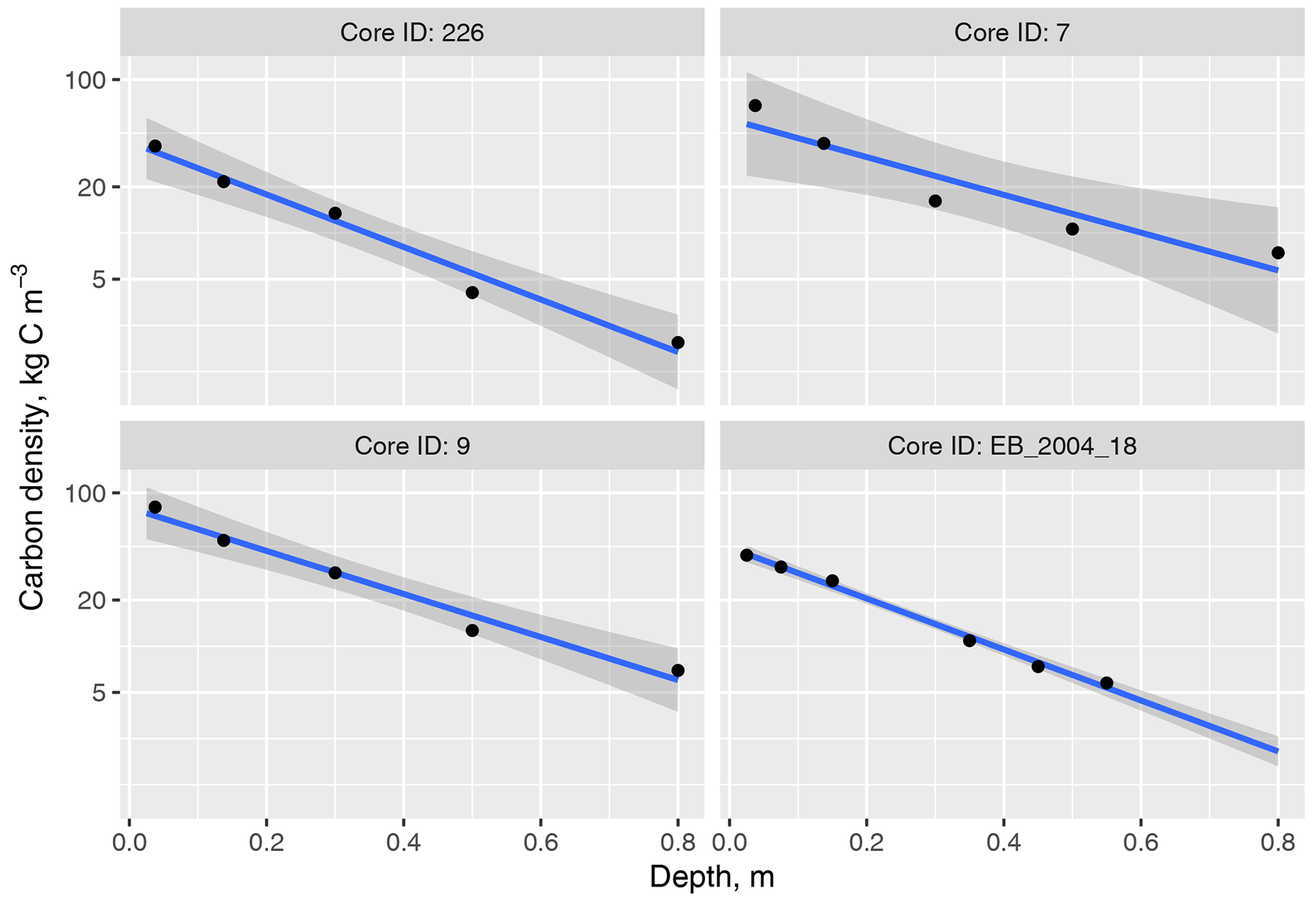
Figure 1 Examples of the relationship between carbon density ρ_c and depth in four soil cores from various sites. Note the logarithmic y-axis scaling. Of the various simple models using different transformations, this gave the best linear relationship. The soil cores come from the surveys of Ward et al. (2016) (samples 226 and 7), ELUM (sample 9), and Easter Bush (sample EB-2004-18), chosen to illustrate the typical range of this relationship. Points represent soil from a depth interval and are plotted against the mid-point of the depth interval.

2.4 Validity of space-for-time substitution

We used two approaches to investigate the validity of the assumption behind the space-for-time substitution. Because we expect increases in S_c which are caused by land-use change to be independent of the initial S_c, we examined whether the ostensible effects of land use are consistent with models of absolute or relative change. The degree of relative change can be equated with the pre-existing difference. To do this, we used the data of Bradley et al. (2005) because the survey includes measurements on multiple land uses on each of several hundred soil series. We expressed the effect of land use as the difference from the value for arable crops on the same soil series; using the land use with the lowest soil carbon stock on average as the reference level means that the overall effects of the three other land uses are positive.

Along similar lines to the above, we explored correlations between altitude and S_c, removing the effect of land use. If S_c increases with altitude and land use also systematically changes with altitude, this relationship could confound our estimate of the effect of land use per se based on the data. To do this, we fitted a simple linear model of S_c as a function of altitude and land use to all the data where altitude was available.

3 Results

Figure 1 shows examples of the relationship between carbon density ρ_c and depth in four soil cores, taken from different sites and surveys. With a logarithmic y axis, a reasonably linear relationship is seen. Variants using logarithmic transformations of x, y, and both x and y axes were explored. The best model in terms of the metrics used (variance explained and the analysis of quantile and residual plots) was the one shown in Fig. 1. In organic soils, reasonable relationships were still seen, but ρ_c was much more constant with depth, so the variance explained by a linear trend was less. We saw some cases where the fit with depth was poorer, indicating soils with more complex vertical structures, such as organic horizons within mineral soils, but these soils were relatively infrequent.

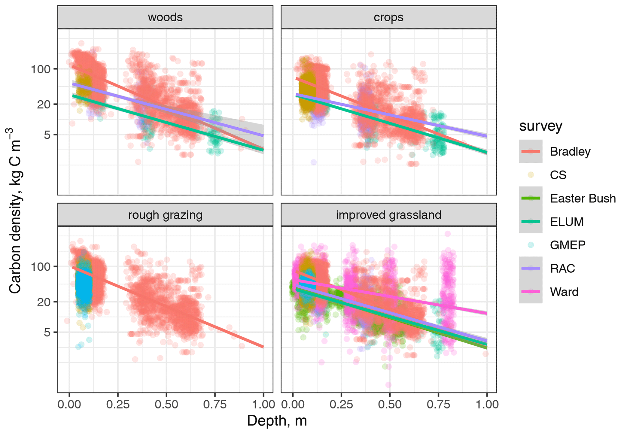
Figure 2 Relationship between carbon density ρ_c and depth by land-use type, showing all data. Note the logarithmic y axis. Points represent soil from a depth interval and are plotted against the mid-point of the depth interval, with some random variation added in the x dimension so that the points are not all overlying each other at a small number of x values. Ordinary least-squares regression lines are shown for each survey.

Table 1 Measures of model fit for three model variants, differing in their specification of the grouping structure. The first column corresponds to a model in which the hierarchical grouping structure (location within site within survey) specifies only an intercept term (so a single global slope with depth is estimated for each land use). The second column corresponds to a model in which the same hierarchical grouping specifies both intercept and slope terms. The third column corresponds to a model in which the hierarchical grouping specifies both intercept and slope terms but only representing variation among locations and sites. The measures are standard deviation (SD) of the residual error, marginal r² excluding the hierarchical grouping terms, conditional r² including the hierarchical grouping terms, Akaike information criterion (AIC), Bayesian information criterion (BIC), intra-class correlation coefficient (ICC), and root-mean-square error (RMSE).

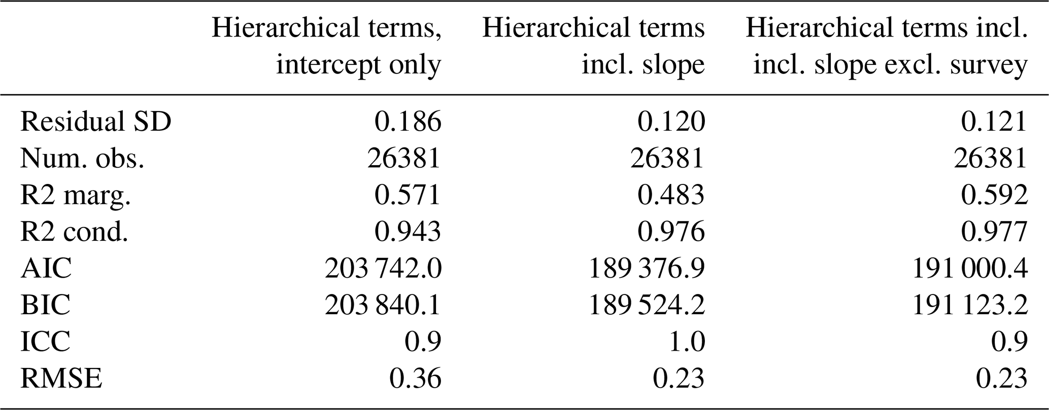
The entire data set is plotted on these same axes in Fig. 2, split by the main land uses. The appearance of a gap in the data at 0.25 m depth is an artefact of the depth intervals chosen in the surveys and plotting using the mid-point of the depth interval. Clearly, there is considerable variation within the main land uses (particularly noting that the y axis is logarithmic). Much of this is accounted for by the group-specific terms in the hierarchical model, such that the full model accounts for more than 90 % of the variance (Table 1). Close to 60 % of this is attributable to the effects of land use and depth, with the remainder attributable to the survey, site, and location group-specific terms. The interpretation of the latter is that there is consistent survey-to-survey, site-to-site, and location-to-location variation in the data, which we can identify and separate from the estimate of the population-level effect of land use. However, the group-specific terms do not represent “explained variance” in the sense that they are not useful for prediction outwith the sample. Ordinary least-squares regression lines are shown for each survey within these groups to identify the broad differences between surveys. The surveys give broadly similar results, but some systematic differences seem to be apparent. The results from Ward et al. (2016) sit higher than the others for grassland; the results from the ELUM survey sit lower. The slope with depth was generally greater in the data of Bradley et al. (2005) than in the RAC survey data, but the mean values were very close. No surveys measured at the same sites, so separating these effects in the model is difficult. With a site-specific effect already accounted for in the model, the additional survey-specific effect made only a small difference to the model selection criteria shown in Table 1. Given that this adds a considerable number of extra parameters to be estimated, we considered this was not warranted and that the form of the model shown in Eq. (8), corresponding to the third column in Table 1, was parsimonious.

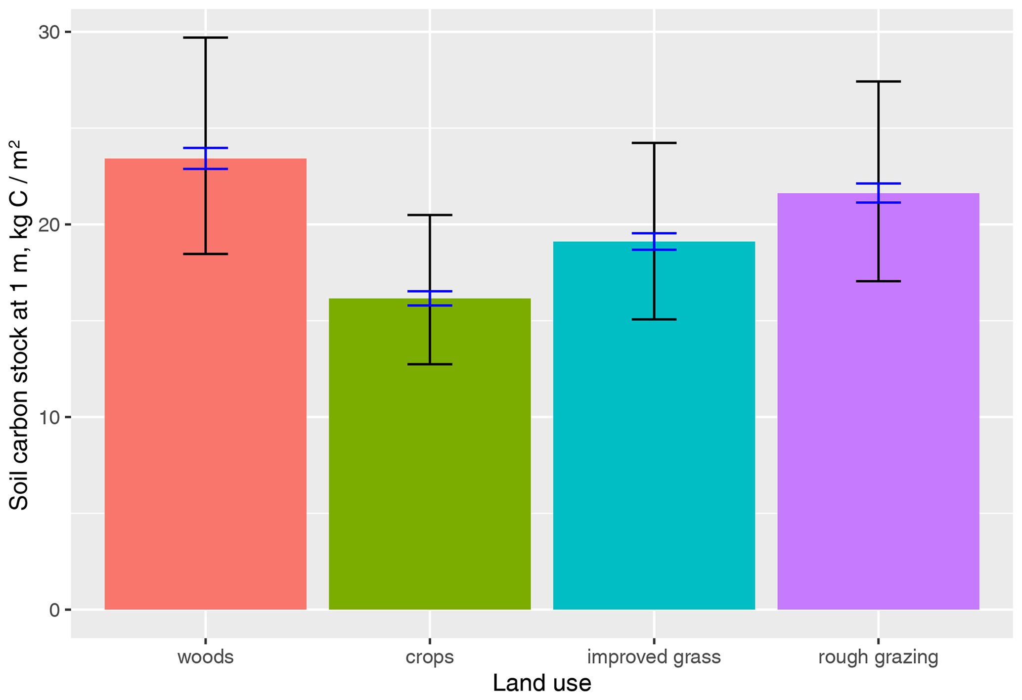
Figure 3 Predicted mean soil carbon stocks to a depth of 1 m for each land use, as estimated by the hierarchical model using all data. Associated 95 % confidence intervals are shown as blue error bars, and prediction intervals are shown in black. Confidence intervals express the uncertainty in the estimate of the true global mean, whereas prediction intervals express the estimated interval in which a new sample would lie with 95 % probability. Both were estimated by a Bayesian estimation of the hierarchical model.

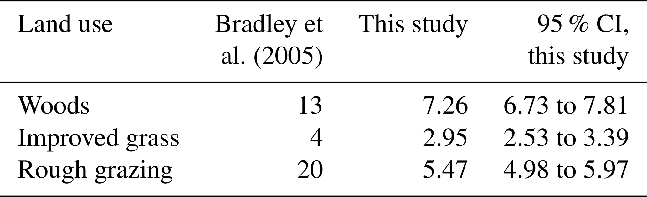
Table 2 Estimates of the effect of land use on soil carbon stock from this study, with 95 % confidence intervals, compared with the estimates reported by Bradley et al. (2005). Effects are expressed relative to arable crops, the land use with the lowest carbon stock, so all effects appear positive. Units are kg C m².

To estimate the mean soil carbon stock for each land use, we use predictions from the model over a depth of 1 m (at z_m where $E\left[{\mathit{\rho }}_c\right]=S_{\mathrm{c},z}$), excluding the site- and location-specific terms (which average out to zero at population level). These are shown in Fig. 3 with associated 95 % confidence intervals and prediction intervals. Soil carbon stocks are highest in woods, followed by rough grazing and improved grasslands, with arable crops having the lowest values. The differences among land uses are larger than the 95 % confidence intervals in all cases, so we can regard these as real, discernible effects. The prediction intervals, which represent the variability in predictions of the effect at a site outwith the sample, are much larger than the effect size.

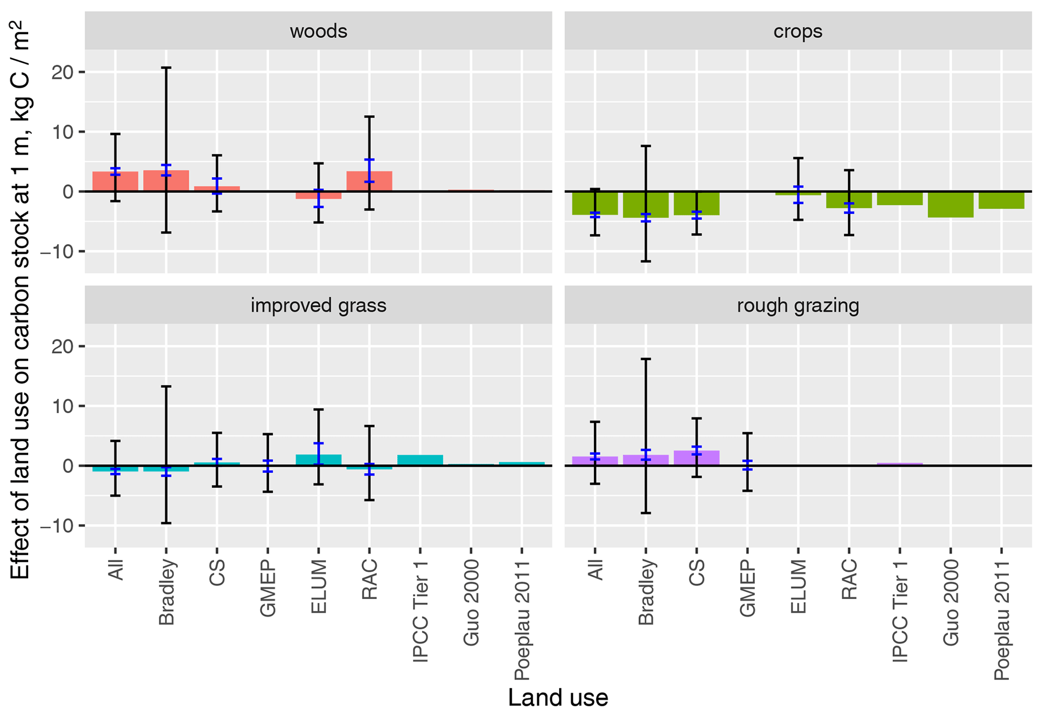
Figure 4 Predicted effect of land use on soil carbon stocks to a depth of 1 m, as estimated by the hierarchical model, expressed relative to the mean soil carbon stock. Associated confidence intervals are shown as blue error bars, and prediction intervals are shown in black. Values are shown for each survey individually and for the full data set. In addition, we plot comparable predictions from the IPCC Tier 1 model and from the meta-analyses of Guo and Gifford (2002) and Poeplau et al. (2011). For the latter, in the case of rough grazing, no comparable values were available, so these are missing rather than zero.

The estimated effects of land use are expressed in Fig. 4 as the difference from the mean soil carbon stock. The effects are estimated from each survey individually and by using all the data. In almost all cases, the effect is of similar magnitude and sign. The sign of the effect appears more variable in improved grasslands, but this lies near the mean, and the degree of variability between surveys is similar to elsewhere, so values may be above or below the mean. The 95 % confidence intervals generally do not include zero, so we can be reasonably sure of the overall effects. The prediction intervals, however, span positive and negative values and are much larger than the effect size.

Also shown are results from three other sources: predictions from the IPCC Tier 1 default method for comparable land-use types, the meta-analysis of Guo and Gifford (2002), and the mean effects from the synthesis of (mostly) paired-plot studies by Poeplau et al. (2011). These all show similar effect sizes to each other and are consistently in the same direction as the UK data. The magnitude of the effect size in arable crops is also very similar to the UK data: that in improved grasslands is close but consistently positive, whereas the UK data are on average lower than the mean (but, as noted above, both lie close to the mean). The effect size for woods is considerably larger in the UK data than in the meta-analyses. The comparison for rough grazing is more restricted, as there is no comparable land use in the meta-analyses, but the IPCC default values are rather lower than the UK data.

Table 2 shows the results of this study compared to the results reported by Bradley et al. (2005), in terms of the effect of land use on soil carbon stock. Because mean values differ between studies, we use the value for arable crops as the reference level: the land use with lowest carbon stock. This does not affect the magnitude of the effects, but it ensures all effects appear positive. Our values are 1.3, 1.7, and 3.4 times smaller than those of Bradley et al. (2005).

In Fig. 5, we examine whether the ostensible effects of land use are consistent with models of absolute or relative change. This shows the apparent size of the land-use effect with increasing soil carbon stock in the data of Bradley et al. (2005). This is expressed as the difference from the value for arable crops on the same soil series so that the overall effects are positive in all three cases. If differences caused by land-use change were independent of the initial S_c, we would expect the horizontal black line, indicating no change in the mean effect size. If there were pre-existing differences within a soil series between land chosen for arable cropping and, say, forestry, these would be expected to be proportional to the soil carbon stock (because the variance in S_c is typically proportional to S_c). This would cause the apparent effect of land use to increase with S_c, and this is what we observe in Fig. 5. The slope is greatest in woods and least in grass, so the magnitude of any error will vary among land uses.

4 Discussion

The results here have improved the estimates of the effects of land use on soil carbon stocks in the UK by increasing the amount of data they are based upon and by providing a more sophisticated analysis which allows the incorporation of soil samples measured at any depth. The Bayesian hierarchical approach allows us to compensate for biases in the choice of sites and protocols used in different surveys and to propagate the associated uncertainty appropriately. Accurate estimates of the soil carbon stocks associated with different land uses is critical to the estimates of emissions from LULUCF, as these differences are the basis of the IPCC methodology.

Because of the large sample size, the data of Bradley et al. (2005) still carry a lot of weight in the overall estimates. However, the new estimates are substantially smaller than the reported estimates of Bradley et al. (2005). We identify a number of factors behind this. The main factor is simply because we use a logarithmic transformation of the carbon density data. This is done for several reasons: it gives an approximately linear relationship with depth, it stabilises the variance so that it is relatively constant with increasing ρ_c, and it makes the model residuals close to normal. The effect is to give less weight to extreme values. Implicit in using a logarithmic transformation is an assumption that the variance is constant in relative, not absolute terms. Whilst the log transformation is a fundamentally better model in this case (because the assumption of relative variance is borne out by the data), it is not a perfect model, and other options are possible: different transformations, Box–Cox transformation, and a generalised linear model with gamma-distributed residuals. All of these would give somewhat different answers, with different weights given to extreme values, and, in reality, there remains epistemic uncertainty as to the best way to summarise the data in the form of a model. A more comprehensive analysis could apply several of these approaches and use a model-averaging approach to indicate the posterior uncertainty that is introduced by this. Clearly this can be considerable, as seen by comparing the results with the previous analysis on the untransformed data.

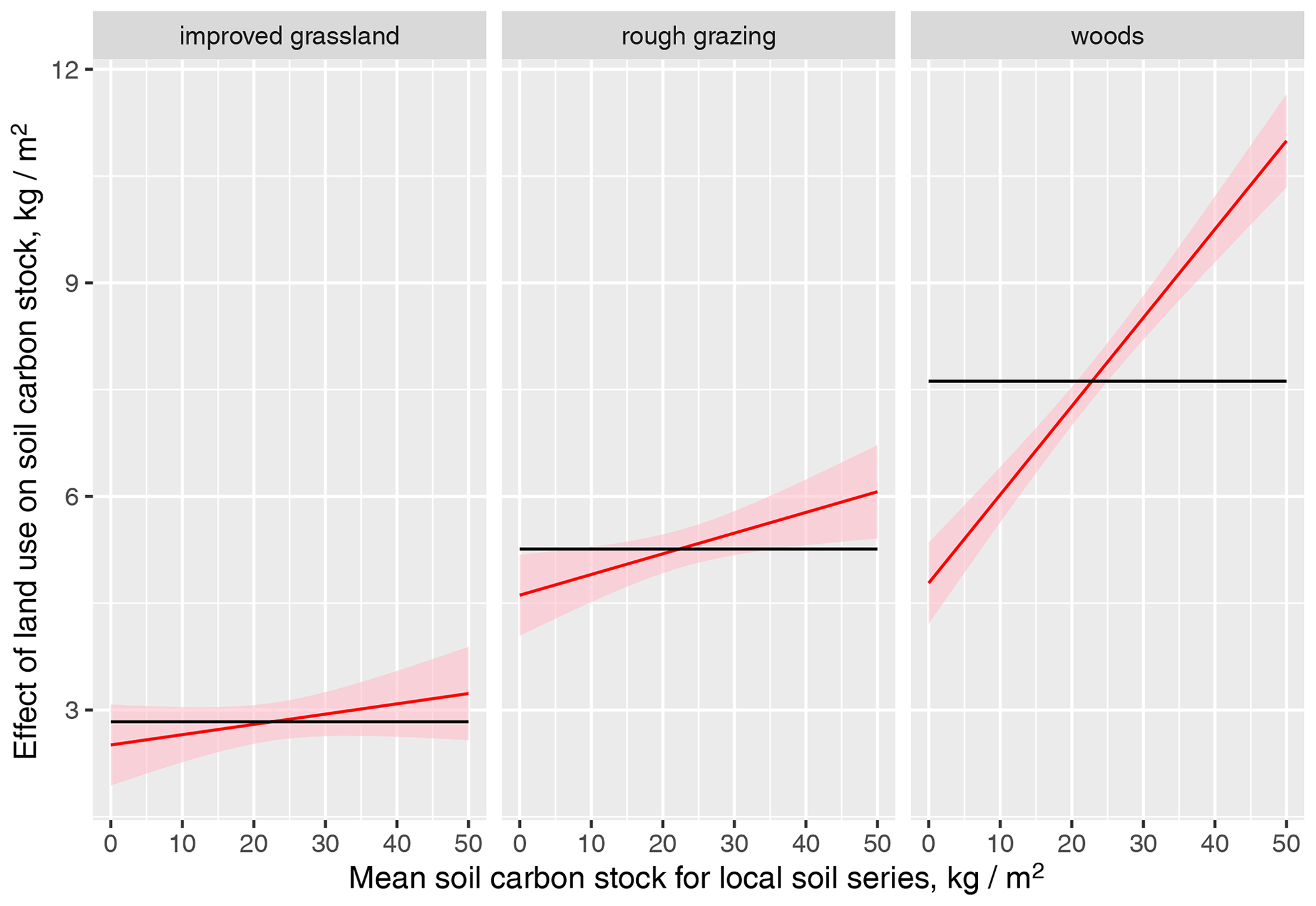
Figure 5 The apparent relationship between the effect of land use and increasing soil carbon stock in the data of Bradley et al. (2005). The effect is expressed as the difference from the value for arable crops on the same soil series so that the overall effects are positive in all three cases. The horizontal black line indicates an expected constant mean effect size in the absence of any effect. Red lines show ordinary least-squares regression lines fitted to the data. The individual data points are not shown because they are highly variable and so require a much larger y-axis scale for display.

A second factor is in the analytical method used by Bradley et al. (2005), which implicitly weighted the effect from each soil series by its area. This would give more weight to the soil series with the largest expanse, although these may have little or no land-use change (e.g. in large areas of the uplands). If this effectively gives more weight towards areas with high soil carbon stocks, and the effect of land-use change is overestimated in these areas for the reasons discussed earlier, then this could introduce a bias. Our approach does not re-weight the data based on estimated areal coverage, and it attempts to estimate the overall effect of land use, having accounted for the vagaries of different sites and soil series. This is a slightly different approach, but it should give the best estimate of the effect at a new location outwith the sample.

The results suggest that the assumption underlying the space-for-time substitution is not completely valid, although they are not unequivocal. The apparent increase in the effect of land use with increasing soil carbon suggests that there are pre-existing differences which confound the comparison, leading us to overestimate the effect. This overestimation varies across land uses, greatest in woods and rough grazing (∼30 % and 15 %, respectively). This tallies with the comparison with meta-analyses of paired-plot studies, which show a smaller effect size. However, the difference is much less in improved grasslands and arable crops, so the effect of pre-existing differences may be much less in these cases. Exploring the trend in soil carbon with altitude, which might lead to an expectation of pre-existing differences in land selected for different uses, showed no strong relationship (although this did not include the Bradley et al. (2005) or the Countryside Survey data). Long-term single-site experiments where changes in land use have been recorded over several decades are still very valuable as a reference point for other analyses. (e.g. the Rothamsted Park Grass Experiment). The Countryside Survey data are important, as they are the result of one of the few long-term surveys with repeated measurements at a spread of locations wide enough to be used to infer national-scale trends. Although these did not include bulk density in the early surveys, so we cannot make strong inferences about S_c, the data show no substantial change in carbon fraction. A more general point is the importance of measuring bulk density when attempting to estimate carbon stock: the fact that this was missing from the data of Bradley et al. (2005), RAC, and the earlier Countryside Surveys make these data sources much more uncertain. Carbon stock is the product of two terms, and one of these terms is missing in these data. Bradley et al. (2005) report a within-sample accuracy of around 10 % in their modelled estimates of bulk density, which propagates directly into estimates of carbon stock. More problematically, there is a high probability of introducing systematic errors when using carbon fraction to predict bulk density (as they did) because the change in this relation (over time or induced by land-use change) is critical but very poorly constrained without simultaneous measurements of both terms. Ideally, all the data would be re-analysed, propagating all the uncertainties appropriately, but the availability of the necessary raw data limits the feasibility of this.

The results show some systematic differences between surveys in estimates of carbon stocks, and this is to be expected for various reasons. Bradley et al. (2005) included all litter horizons in their definition of soil, whereas the Countryside Survey and GMEP included only the F (folic, partially decomposed) and H (humic, decomposed) layers and excluded the readily recognisable litter. Differences in the attribution of litter material to the soil have been noted before as a key difference between soil survey schemes and as an important factor for consistency in experimental comparisons, particularly in wood and forest environments (Poeplau et al., 2011). This may explain why the data of Bradley et al. (2005) show higher carbon densities in woodlands compared to the Countryside Survey, with the greatest difference in woodlands. The effect is less pronounced in other land uses where there is less litter. This may explain some of the difference shown in the comparison of the effect of woodland land use among surveys (Fig. 4) and in Table 2, although the effect of log transformation is the dominant difference here. There will also be differences among surveys caused by differences in laboratory analytical procedures. Various authors have shown effects of sample mass, combustion temperature, and duration on the mass loss observed in the loss-on-ignition method, particularly highlighting the extent of structural water loss and its dependency on clay content (e.g. Hoogsteen et al., 2015). Heming (2021) rejects the method on the basis of the uncertainty introduced by the latter. Similarly, the elemental analyser approach is prone to the uncertainties associated with separating organic and inorganic carbon (Wang et al., 2012), and this will introduce a different set of biases. Consistency is key in long-running survey schemes so that true changes over time can be separated from changes related to different analytical methods. The hierarchical statistical method used attempts to remove such effects, partitioning them into group-level effects rather than viewing them as part of the overall effect of land use which we are trying to discern.

Soils vary widely in depth, and the modelling approach used here makes the comparison across a standardised depth of 1 m, based on the guidelines for UNFCCC reporting. Many soils in the UK are shallower than this: around half the soils in Wales are in classifications with a lithoskeletal substrate, which define the soil to be less than 80 cm thick. We note that the results should be interpreted as predictions of the effect of land use on a typical but hypothetical soil of 1 m depth, taking into account the way in which carbon density declines with depth. A more complex model would be required to make accurate spatial predictions.

Cropland soils are typically ploughed to a depth of around 30 cm. This means that the top layer will be repeatedly mixed with soil from below and could reduce the slope of soil carbon versus depth because of the mixing effect of the plough. Furthermore, the effect of ploughing might be to create two different layers (above and below the plough depth) with different slopes (soil carbon vs. depth), so something like a “broken-stick” model might be more appropriate. In fact, we do not see evidence for either of these effects in the data, but this may be because the samples lack the vertical resolution to discern such trends. Given the level of aggregation in the available data, the logarithmic decline appears to be reasonable.

With the large data set analysed here, the uncertainty in the differences among land uses was small enough to identify consistent mean effects. However, a striking feature of the results is the extent of the variability in these effects, represented by the large prediction intervals, and this was similar across all surveys. Mapping soil carbon using geostatistical or machine learning methods has become widespread and increasingly accurate because of the strong spatial relationships in the data (Hengl et al., 2017). However, this may lead to a false sense of understanding of causal relationships. The data here highlight the degree of variability, and the effects of land use, whilst discernible in very large samples, are not as clear as is generally pre-supposed (Baker et al., 2007; Kravchenko and Robertson, 2011). This has important consequences for attempts to verify schemes which aim to sequester carbon in the soil by altering land use.

With pressure to find measures which will help meet targets for net-zero emissions, there is now considerable interest in options for sequestering carbon in agricultural soil (Soussana et al., 2019; Alliance, 2022). To be credible, these options will need to be verifiable and governed to ensure permanence and prevent leakage or reversals (Smith et al., 2020; Black et al., 2022). If soil carbon credits are to be used to pay farmers for changes in land use or management, the effects need to be demonstrable over relatively short timescales and at a practicable cost. The results we find here have implications for the prospects for this. Although we can demonstrate an overall mean effect greater than the uncertainty bounds with a large sample size (more than 25 000 individual samples (core depth sections) at several thousand locations), we find that the variability in these effects is much larger. The prediction intervals were much larger than the mean effect size, and they spanned both positive and negative effect sizes. This result was consistent across all the surveys we analysed. In any given instance where we wish to verify the change in soil carbon, our expectation is that the observed change in soil carbon will lie in a very wide range, encompassing both possible gain and loss. Indeed, there will often be instances where the observed effect is opposite to the expected mean effect. The effect of a given intervention is therefore very hard to verify, and this raises questions on how this might be handled in such schemes as a formal part of efforts to mitigate climate change.

The effect of the changes to the estimates of equilibrium soil carbon on the carbon fluxes arising from land-use change is not obvious. The changes will reduce the gross fluxes from each land-use change, but how this affects the net effect depends on the balance of changes and the transition matrix of land-use change each year (Levy et al., 2018), so the net effect is not linearly predictable and requires further analysis.

5 Conclusions

We have produced new estimates of the effects of land use on soil carbon stocks in the UK. These are smaller than the previous best estimates of Bradley et al. (2005), partly because of new data but mainly because the effect is more reliably characterised using a logarithmic transformation of the data. We characterised the uncertainty and variability in the effect. With the very large data set analysed here, the uncertainty in the differences among land uses was small enough to identify consistent mean effects. However, the variability in these effects was large, and this was similar across all surveys. This has important consequences for attempts to verify schemes which aim to sequester carbon in the soil by altering land use. Whilst we can estimate the expected overall effect at national scale, the effect in any given instance is expected to lie in a very wide range. The effect of a given intervention is therefore very hard to verify and may be difficult to include as a formal part of efforts to mitigate climate change. Examining whether the “space-for-time” substitution is valid, the results were not unequivocal, but we estimated that the effects are likely to be overestimated by 5 %–33 %, depending upon land use.