Forestlines in Italian mountains are shifting upward: detection and monitoring using satellite time series

The growing interest on the ecological effects of global warming and land use changes on vegetation, along with the development of remote sensing techniques, fostered applied research on the successional dynamics at the upper limits of forests. The aims of this study are (i) to develop an automated methodology for mapping the current position of the uppermost Italian forestlines and (ii) to identify hotspots of change by the analysis of long-term greenness and wetness spectral dynamics. We carried out a Landsat-based trend analysis in buffer zones along the forestlines, testing differences between sparse and dense canopy cover classes and at different elevations and distances to the forestline. We used regional-scale datasets and avoided to fix a minimum elevation threshold for the detection in order to make the method replicable in different mountain ranges. For the spectral dynamics analyses, we used Landsat time series of common vegetation indices for the period 1984–2023 and tested the significance of their long-term spectral trends with the contextual Mann–Kendall test for monotonicity. We determined that the highest forestlines are located in the western Alps for the Alps mountain range and in the central sector for the Apennines. We observed a general expansion of the forest cover mainly close to the forestline and at lower elevations. The highest values of greenness and wetness indices were, respectively, in the sparse tree cover class and in the dense one, particularly in the Alps.

1 Introduction

A treeline is the contiguous forest–grassland ecotone along an altitudinal or latitudinal gradient (Körner, 2008; Berdanier, 2010; Harsch et al., 2011). Nowadays, most treeline studies concern the response of spatio-temporal dynamics to climate and/or land use changes (Malanson et al., 2011). Current treeline elevation and its spatial patterns derive from air temperature increase and past human activities that have modified their physiognomy and dynamics over time (Holtmeier et al., 2005; Harsch et al., 2011). Most European mountain landscapes have been shaped since prehistoric times through fire, deforestation, and intensive grazing (Malanson et al., 2011; Vitali et al., 2018; Garbarino et al., 2020). In the Mediterranean region, the treeline elevation is much lower than its potential climatic position (Körner 2012; Piper et al., 2016). Moreover, human activities have locally altered, directly or indirectly, species composition (Obojes et al., 2024) and induced new disturbances as the in the western Alps, favoring Larix decidua Mill. to Pinus cembra L. and promoting an invasive resprouter like Alnus viridis (Chaix) DC. (Motta et al., 2006; Dziomber et al., 2024). In the Apennines, Pinus nigra J.F. Arnold plantations at higher elevations facilitated its upward encroachment in treeline ecotones (Vitali et al., 2017). The upward treeline shift occurring in many parts of the globe can therefore be associated with not only global warming (Hansson et al., 2023) but also successional dynamics (Ameztegui et al., 2016; Vitali et al., 2017) and geomorphic processes (Leonelli et al., 2009).

The development of remote sensing techniques and geographic information systems provided new opportunities in treeline studies (Holtmeier et al., 2020) such as detecting and monitoring the dynamic patterns of treeline shape and density (Fissore et al., 2015). Defining clear and easily replicable methods based on the application of modern technologies to access available datasets is fundamental for accurate and large-scale treeline monitoring. At the local scale, aerial photography is commonly used (Ameztegui et al., 2016; Hansson et al., 2020; Nguyen et al., 2024) since it provides older images than satellite ones, although image quality and availability are limiting factors (Morley et al., 2018). At larger scales, He et al. (2023) detected closed-loop mountain treelines integrating high-resolution tree cover maps and digital elevation models, whereas Wei et al. (2020) in the western United States proposed an “alpine treeline ecotone detection index” (ATEI) based on the analysis of altitudinal and normalized difference vegetation index (NDVI) gradients. At the regional scale, supervised and unsupervised classification of multispectral images are widely used (Fissore et al., 2015; Chhetri and Thai, 2019), as well as detection techniques based on land cover maps combined with digital elevation models (e.g., Pecher et al., 2011).

Besides mapping, current treeline research includes also its spatio-temporal dynamics. Despite the coarser spatial resolution and the limitation of cloud cover, satellite optical imagery offers a finer time resolution by integrating data from several platforms and free processed time series. It also provides spectral information for synchronic analysis of vegetation changes (Gómez et al., 2016). The free access to its database in 2008 has increased the use of Landsat time series (Zhu, 2017). Given their spatial resolution (30 m) and temporal data availability, Landsat images have been largely used for vegetation dynamics monitoring, such as post-disturbance forest recovery (Morresi et al., 2019) and greening or browning in different ecosystems (Kumar et al., 2022; Rumpf et al., 2022; Bayle et al., 2024), and to study alpine treelines by applying greening proxies like vegetation indices (Fissore et al., 2015; Tian et al., 2022). The NDVI is widely used in treeline dynamics monitoring, being more sensitive in detecting biomass changes in open rather than in closed canopies (Bharti et al., 2012; Arekhi et al., 2018; Wei et al., 2020; Choler et al., 2021; Zou et al., 2022; Bayle et al., 2025). In the European Alps, Carlson et al. (2017) and Choler et al. (2021) used the annual peak values of NDVI (NDVI-max) to analyze the greening trends from Landsat and MODIS time series. They assessed a significantly increasing spectral trend over the last 2 decades, mainly at north-facing slopes and in sparsely vegetated areas. Nevertheless, Bayle et al. (2024) remarked that the higher number of Landsat observations throughout the growing seasons can affect the NDVI-max trend analysis, causing false outcomes. It is true that annual NDVI-max increase with the number of available observations, and therefore their frequency must be taken into account. In the southwestern part of the European Alps, Bayle et al. (2025) studied greening trends using the annual max of the kernel normalized difference vegetation index (kNDVI) (Camps-Valls et al., 2021), a nonlinear version of the NDVI, overcoming the overestimation of greening by the harmonic analysis of time series (HANTS), as reported by Choler et al. (2024). Bolton et al. (2018), instead, used the enhanced vegetation index (EVI) for a Landsat-based greening trend analysis of alpine treelines in the Canadian boreal zone. The EVI corrects the aerosol influence and canopy background noise, and it is less affected by saturation than NDVI, being more sensitive to the near-infrared (NIR) band (Huete et al., 2012). For this reason, it can detect the spectral behavior of lower layers of vegetation, while the NDVI responds mainly to the RED band, which is involved in photosynthetic activity of the upper canopy layer. A single index can be combined with other vegetation indices to reduce the uncertainty in change detection analysis (Schultz et al., 2016; Zhou et al., 2023). EVI and NDVI can be considered greenness indices since they are linked to the photosynthetic activity of vegetation using NIR and RED bands, while wetness indices introduce shortwave infrared (SWIR) bands that are especially sensitive to the water content of vegetation (Huete, 2012). Examples of wetness indices are the normalized difference moisture index (NDMI) and the normalized burn ratio (NBR) index. Such indices are sensitive to shadowing, forest structure, leaf internal structure, vegetation moisture and density (Schroeder et al., 2011). In Landsat-based forestry applications, indices derived from the tasseled cap transformation (TCT) (Kauth and Thomas, 1976; Crist and Cicone, 1984) are also commonly used, since they are less affected by soil reflectance (Cohen and Goward, 2004). The tasseled cap wetness index (TCW) considers the visible bands and both SWIR1 and the SWIR2, and it is suitable to predict forest structural attributes, being slightly influenced by topographic variations, especially in closed conifer stands (Cohen et al., 1995). Another TCT index is the tasseled cap angle (TCA) (Powell et al., 2010), combining the greenness and brightness information as defined in Crist and Cicone (1984) to assess the ratio between vegetated and non-vegetated areas (Gómez et al., 2011). In this study, we consider the “forestline” to be the line separating the closed forest from the shrubland and grassland above and the “treeline” or “forestline ecotone” to be the surrounding area, the spatial pattern of which was not investigated due to the scale of analysis adopted. Forestline ecotones are dynamic ecosystems, and their monitoring at regional scale can be conducted with the analysis of their spectral behavior over time adopting different indices and tools. In this context, our study analyzed forestline dynamics of the two main Italian mountain ranges, the Alps and the Apennines. Our research aims were

1. to define and monitor the position of the uppermost forestlines with an automated methodology;

2. to identify hotspots of change through satellite data, verifying whether and where forest recolonization dynamics are occurring.

In particular, we analyzed the long-term greenness and wetness spectral changes of the uppermost forests and the contiguous forestline ecotones using a Landsat-based trend analysis of time series for the period 1984–2023, and we tested if greenness and wetness indices trends differed with elevation, forestline distance, and canopy cover densities. We hypothesized that greenness indices are more fitted for forest recolonization of open areas, while wetness indices are better suited for detecting gap-filling processes by intercepting also the spectral signal of lower leaf strata.

2 Materials and methods

2.1 Study area

The Alps and the Apennines are the two major mountain ranges of the Italian peninsula. They extend, respectively, for 1300 and 1350 km: the Alps from west to east across northern Italy; the Apennines from the northwest to the southeast. They differ in climate, elevation range, and vegetation characteristics. In the Alps, annual precipitation ranges between 400 and 3000 mm, with rare summer dry periods and cold winters (Isotta et al., 2014). Conifer forests prevail in the subalpine zone, where the main species are Norway spruce (Picea abies (L.) H. Karst.), European larch (Larix decidua Mill.), and Swiss stone pine (Pinus cembra L.) (Fauquette et al., 2018). In the Apennines, the total annual precipitation ranges between 600 and 4500 mm (Vacchiano et al., 2017), with short and pronounced summer dry periods (Blasi et al., 2014). Mixed broadleaf forests dominate at lower elevations, while common beech (Fagus sylvatica L.), locally mixed with silver fir (Abies alba Mill.), is the main species in the montane zone, except for rare locations in the central and southern Apennines, where also mountain pine (Pinus mugo Turra), European black pine (Pinus nigra J. F. Arnold), and Bosnian pine (Pinus heldreichii H. Christ) occur naturally. With the Italian forestline ecotones being the target of our study, we selected the highest peak for each mountain group of the Alps and of the Apennines, as defined by the Global Mountain Biodiversity Assessment (GMBA) inventory (Snethlage et al., 2022a, b). We located the exact position of the peaks using the nationwide Tinitaly digital elevation model (DEM) v 1.1 (Tarquini et al., 2023) that is a DEM with a 10 m spatial resolution obtained from the union and harmonization of each Italian administrative regions' digital terrain models. We then filtered the mountain groups and retained only the ones with the highest peaks located on bare soil or in snow-/ice-covered areas according to the Dynamic World land cover map (Brown et al., 2022). In this way, we excluded also the mountain groups completely covered by forest or affected by severe human impacts, such as urbanized areas or areas with settlements. In addition, for excluding the mountain peaks lacking the alpine belt thermoclimatic features, we used the oro-temperate, cry-oro-temperate, and gelid thermotypes derived from the Bioclimates of Italy dataset (Pesaresi et al., 2017) based on the Worldwide Bioclimatic Classification System (WBCS) by Rivas-Martínez (1993). Other GMBA mountain groups have been removed after the previous selection based on land cover and bioclimatic parameters because the Italian administrative and GMBA's boundaries limited the altitudinal range and forest distribution of some groups on the border in the following analyses (Sect. 2.2).

2.2 Detection of forestlines

We used the Tree Cover Density 2018 (TCD) dataset of the European Environment Agency (EEA) derived from Sentinel-2 multispectral data as a reference for forest cover (Copernicus Land Monitoring Service, 2024). TCD has a 10 m spatial resolution and provides information about the percentage of crown coverage in each pixel with a minimum thematic target producer and user accuracies of 90 % (EEA, 2025). According to the FAO “forest” definition (FAO, 2000), we selected only pixels with a TCD higher than 10 % to obtain a mask of forested areas. For each mountain group, we obtained the vertical distance between each forest pixel and the DEM-derived highest peak. We then selected the forest pixels with a vertical distance within the first percentile of all the distances and extracted the contours of the forestline by considering only the side of each selected forest pixel facing the mountain peak. We avoided a minimum elevation threshold for the forestline detection to facilitate the replicability of the method in geographic regions with different altitudinal ranges. We joined polylines with linear gaps shorter than 30 m (corresponding to the Landsat spatial resolution). We considered only resulting polylines longer than 500 m to avoid highly fragmented forestlines and to focus on more spatially extended and continuous ecotones, and we removed closed loops to exclude the edges of forest gaps below the forestline. We defined a buffer zone of a 250 m radius (Fig. 1c) along the forestlines to assess the presence of significant spectral changes in a gradient from closed forest to grassland. We also sampled points at 10 m intervals along the detected forestlines to assess the mean, median, and maximum elevation of all of them clustered by mountain groups or ranges. We processed the data in the R software environment (v. 4.3.2), using the “terra” (Hijmans, 2023), “callr” (Csárdi and Chang, 2024), and “future.apply” (Bengtsson, 2021) packages, and with QGIS software (v. 3.34.1).

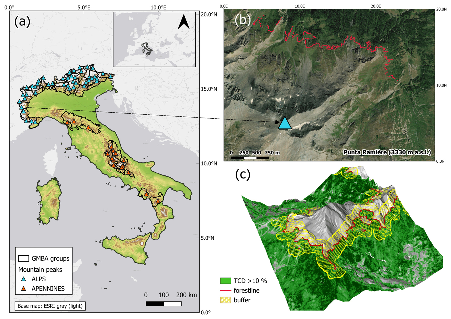
Figure 1 (a) Selected peaks (triangles) along the Italian Alps (light blue) and the Apennines (orange). (b) Detected forestlines (red polylines) on an ESRI satellite image (ArcGIS/World_Imagery) of Punta Ramière (3330 m a.s.l.) in the Montgenèvre Alps GMBA group. (c) a 3D graphical model based on the Tinitaly DEM and the TCD forest mask (TCD >10 %) used for the forestline detection and the buffer area definition (yellow area).

2.3 Trend analysis of vegetation indices

Sentinel-2 provides images with a higher spatial resolution (10 m) but a shorter time span (since 2018) than Landsat. In fact, Landsat images have supplied multispectral information at medium resolution (30 m pixel size) since 1984 and are commonly used in treeline studies (Bharti et al., 2012; Arekhi et al., 2018; Morley et al., 2019; Garbarino et al., 2023) since they give a good compromise between space and time resolution at regional scale (Hansson et al., 2020). We collected Landsat images acquired from 1 June to 30 September of each year in the period from 1984 to 2023 to analyze forest vegetation dynamics during the growing season. In particular, we used Level-2 Collection 2 Landsat images acquired by the TM, ETM+, OLI, and OLI-2 sensors. After masking pixels covered by snow, clouds, cloud shadows, and water, we produced pixel-based reflectance composites based on the medoid compositing approach (Flood, 2013). We preferred the medoid technique over the traditional compositing approaches because it is more robust to outliers and noise. In fact, it consists of the closest value to the median. We computed common vegetation indices from reflectance composites that we grouped into (i) greenness indices – normalized difference vegetation index (NDVI) (Tucker, 1979), enhanced vegetation index (EVI) (Huete et al., 2002), and tasseled cap angle (TCA) (Powell et al., 2010) – and (ii) wetness indices – normalized burn ratio (NBR) (García et al., 1991), normalized difference moisture index (NDMI) (Gao, 1996), and tasseled cap wetness (TCW) (Crist, 1985). Finally, we masked the 40-year-long time series using the buffer areas around each selected forestline (Sect. 2.2).

We assessed the significance in the monotonicity of the spectral trends, i.e., strictly increasing or decreasing, derived from vegetation indices time series by applying the nonparametric contextual Mann–Kendall (CMK) statistical test (Neeti et al., 2011). The CMK test is an estimator of the monotonicity of trends based on the Mann–Kendall (MK) test, which takes into account the trends in the neighboring pixels within a 3 × 3 kernel. In this way, the spatial autocorrelation is considered, thus improving the detection of spatial patterns characterized by homogeneous spectral trends. Specifically, we used the ConMK R package (Rajala, 2024). The TAU statistics produced by the MK test ranges between +1 and −1, with positive values indicating an increasing trend, while negative values are associated with decreasing trends. Before checking the occurrence of significant trends by computing the p value (α) associated with the TAU statistics, we pre-processed time series in two steps. Firstly, we filled 1-year data gaps at the pixel level through linear interpolation while discarding pixels with longer data gaps. Secondly, we removed the autocorrelation in the time series by applying the “pre-whitening” procedure proposed by Wang and Swail (2001) and implemented in the ConMK R package.

2.4 Assessment of the spectral trends

For each group of vegetation indices, i.e., greenness and wetness, we selected only those pixels that exhibited a highly significant trend (α<0.005), as proposed in Choler et al. (2021) for all the indices (Fig. 2).

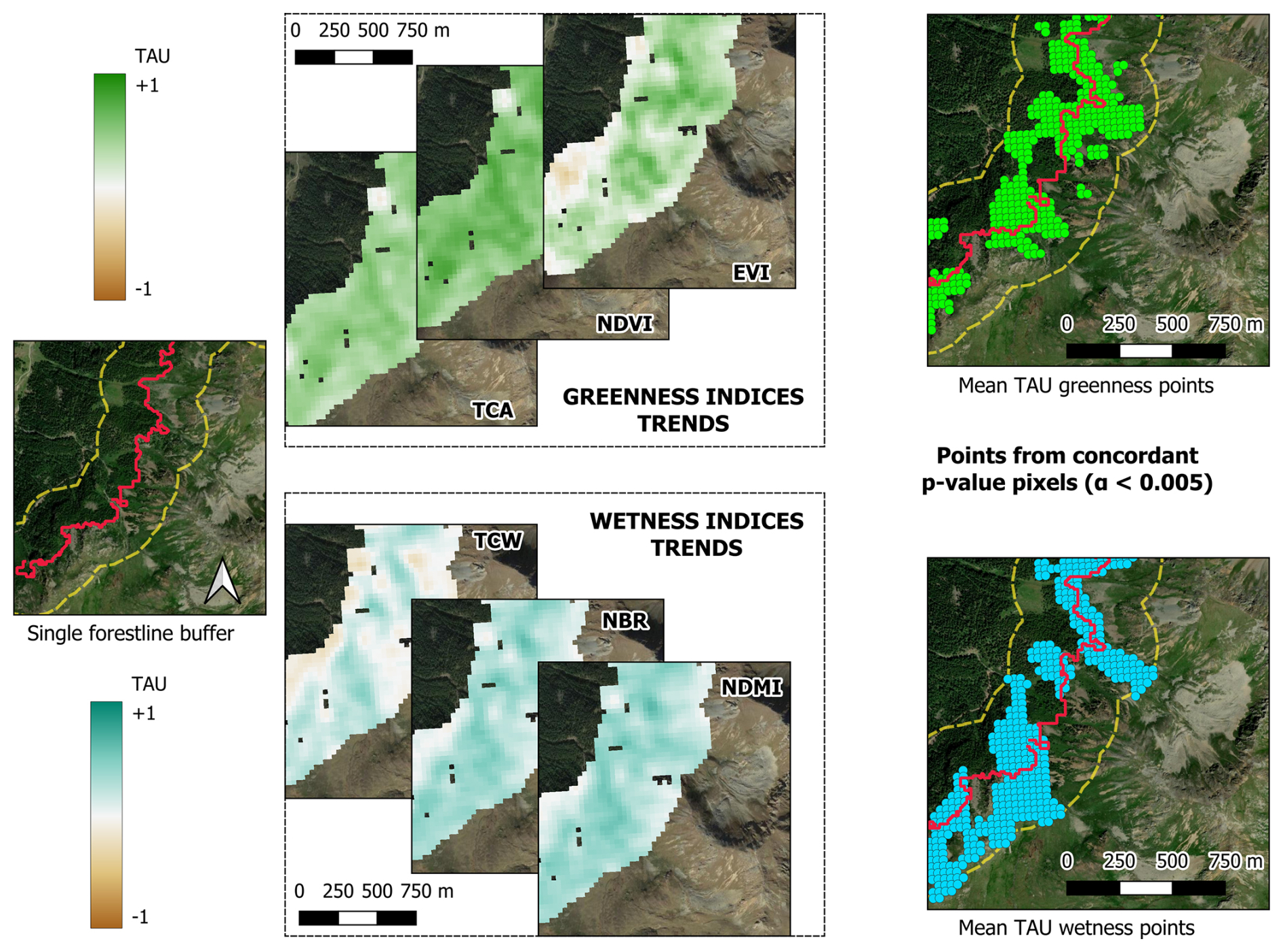
Figure 2 Example of the extraction of the highly significant (α<0.005) greenness (top) and wetness (bottom) points trends in the buffer area (yellow dotted line) around a single forestline (full red polyline) in the Alps. Base map: ESRI Satellite (ArcGIS/World_Imagery).

We used the points corresponding to the resulting pixel centroids to extract the mean TAU value among the vegetation indices and the elevation from the Tinitaly DEM. The original TCD excludes shrublands, dwarf pine, or green alder in alpine areas (EEA, 2025), but we resampled it to 30 m by average and assigned to each pixel centroid also the mean tree canopy cover. We excluded points with negative trends (TAU <0), and with TCD = 0, that corresponded to areas without a tree canopy cover (e.g., grasslands) and where the significant increasing spectral trend of the last 40 years was probably due to factors and dynamics different from forest recolonization. We assigned the elevation value of the nearest forestline point to the resulting wetness and greenness points using the “join attributes by nearest” tool in QGIS. In this way, we obtained the Euclidean distance of each trend point to the forestline and the elevation difference, which we used to classify the points above or below the forestline. In particular, we identified the relative position of each point to the forestline by multiplying the Euclidean distances by the sign of the elevation difference. We carried out the analysis separately for the Alps and the Apennines given their altitudinal, climatic, and vegetation differences. After this characterization of the trend points, we randomly sampled two sets of 40 000 points for each mountain range by the “slice_sample()” function of the “dplyr” R package (Wickham et al., 2023). Each set contained an equal number of greenness and wetness significant trend points. We then grouped the sampled points into three tree canopy cover categories according to TCD: (i) sparse canopy cover (TCD < 10 %), (ii) moderate to dense canopy cover (10 % < TCD < 80 %), and (iii) dense canopy cover (TCD > 80 %). Because of the large canopy cover classes ranges to which the points were allocated taking into account a mean TCD value, a possible spatial mismatch between the resampled TCD and the Landsat data was ignored. We then assessed the relationship between TAU values and the canopy cover, the elevation, and the distance to forestline, taking into account the mean values of each forestline segment. We used a Wilcoxon test (Wilcoxon, 1945) to verify significant differences between the mean TAU among wetness and greenness indices, averaging the mean TAU values of each canopy cover class in each forestline buffer. Finally, we built generalized additive models (GAMs) (Hastie and Tibshirani, 1990) using the cubic spline smoother of the “mgcv” R package (Wood, 2011) to test the presence of a significant nonlinear relationship between the mean TAU values and (i) the elevation and (ii) the forestline distance without considering the TCD classes.

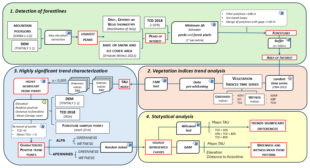
Figure 3 Flow chart of the analytical process: input data (black rectangles), outputs (red rectangles), and statistical analyses (irregular rectangles). Abbreviations: DEM (digital elevation model), TCD (tree cover density), NDVI (normalized difference vegetation index), EVI (enhanced vegetation index), TCA (tasseled cap angle index), NDMI (normalized difference moisture index), NBR (normalized burn ratio), TCW (tasseled cap wetness), CMK (contextual Mann–Kendall test), and GAM (generalized additive model).

3 Results

3.1 Forestline extraction

We identified and processed 60 mountain peaks, 44 in the Alps and 16 in the Apennines (Table A1, Appendix A). We obtained approximately 5760 km of forestlines with a mean elevation of 2088 ± 193 m a.s.l. in the Alps and 1758 ± 161 m a.s.l. in the Apennines, with a maximum elevation, respectively, of 2500 and 2383 m a.s.l. In the Alps, the lowest forestline elevations were in the prealpine groups due to the lack of a suitable altitudinal gradient, whereas the highest ones were mainly in the western sector (Fig. 4a). In the Apennines, the lowest and less extended forestlines, if compared to the forested areas, were in the northern sector, while the highest ones were in central Italy: the Majella (MJ), Sirente Velino (SVE), and Marsicani (MM) mountain groups (Fig. 4b). The total area of interest extended approximately for 1880 km².

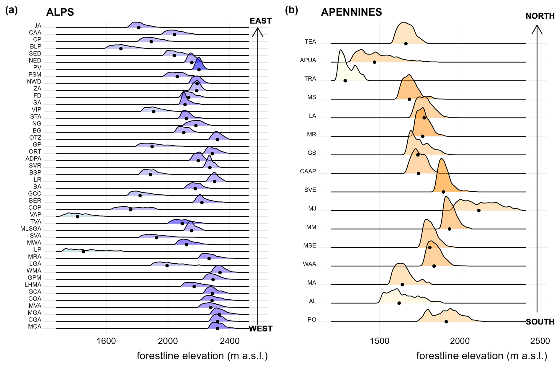
Figure 4 (a) Forestline elevation ranges of the mountain groups in the Alps (n=44) sorted by longitude (west–east). (b) Forestline elevation ranges of the mountain groups of the Apennines (n=16) sorted by latitude (south–north). Black dots are the median values of each interval; the color intensity of ridges increases with forestline length and forested area ratio. Mountain group codes are available in Table A1 (Appendix A).

3.2 Trend analysis and performances

We obtained 28.81 % of highly significant (α<0.005) trend pixels for greenness and 19.69 % for wetness, considering only pixels with concordant p values on all of the indices. The majority of TAU values were positive (Fig. 5) at both index types, with, respectively, 97.8 % and 99.8 % in the Alps and 96.3 % and 99.7 % in the Apennines.

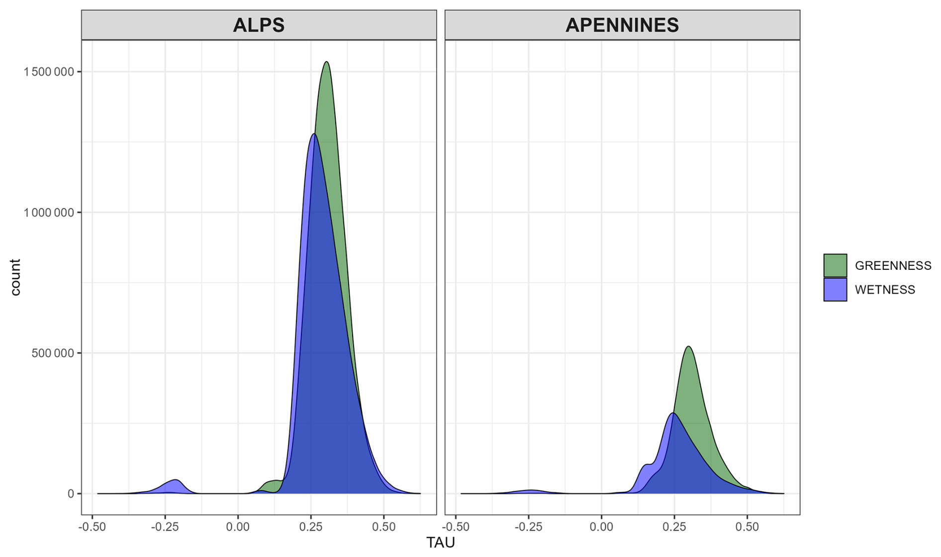
Figure 5 Distribution of the highly significant (α<0.005) wetness (blue) and greenness (green) pixel frequency with different TAU values.

In total, we obtained 242 233 greenness and 221 554 wetness highly significant positive trend pixels for the Alps and 76 348 and 508 745, respectively, for the Apennines. With sparse and moderate to dense canopy cover, the greenness and wetness positive trends were mainly near the forestline in both mountain ranges and decreased in both directions, but mainly upward where tree-covered areas are gradually replaced by high-altitude grasslands. With dense canopy cover, only wetness positive trends in the Apennines showed a similar distribution, differently from greenness trends and from both types in the Alps, where the highest concentration was below and distant from the forestline (Fig. 6).

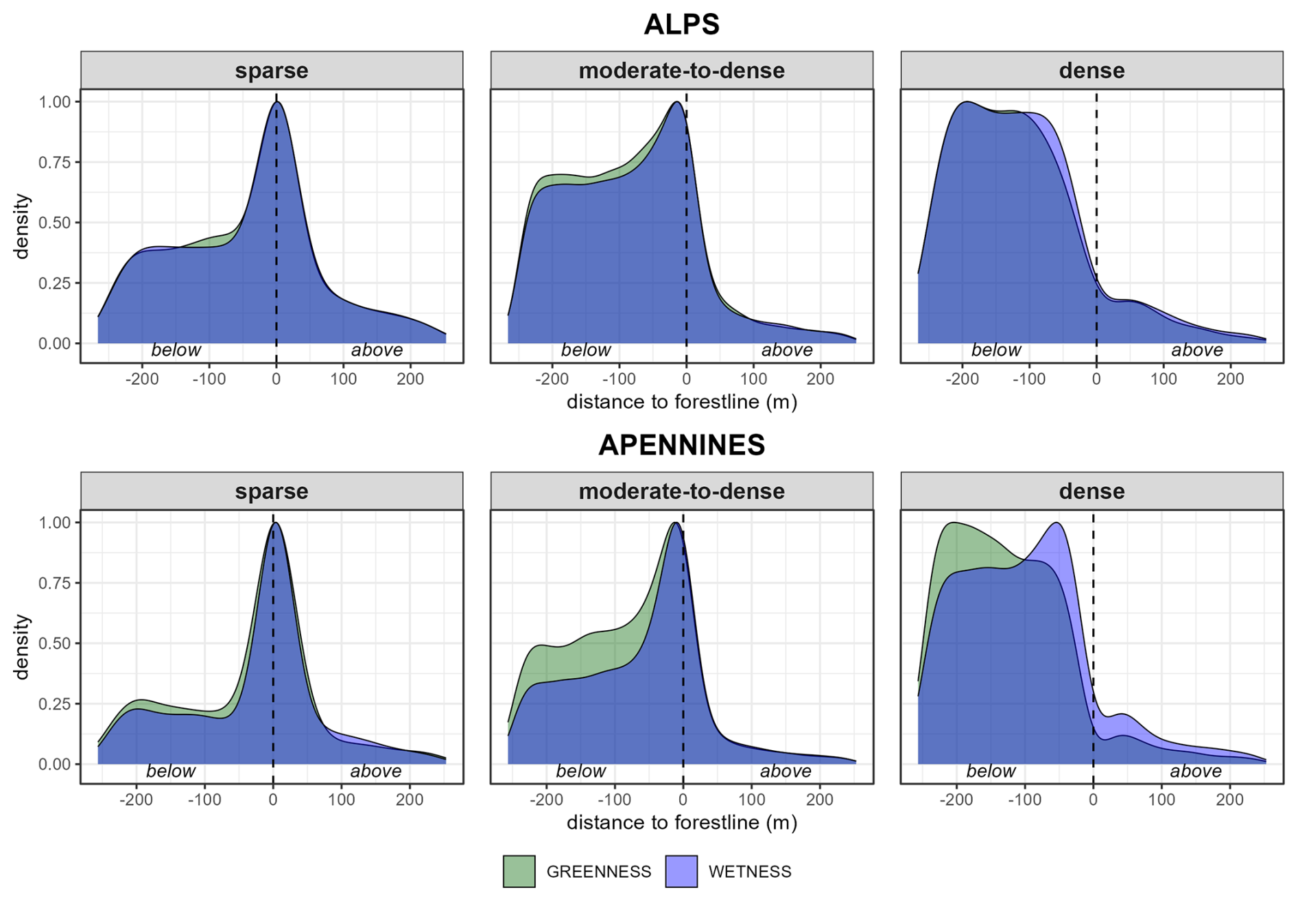
Figure 6 Positive wetness (blue) and greenness (green) trend pixel density according to their distance to the forestline (black dashed line) in different canopy cover classes: sparse (TCD < 10 %), moderate to dense (10 % < TCD < 80 %), and dense (TCD > 80 %). Negative and positive values represent distances below and above the forestline, respectively.

Significant differences between TAU trends and canopy cover classes occurred mainly in the Alps (Fig. 7). The highest ones were for the wetness indices in the dense canopy cover. For greenness, sparse canopy cover class had a higher mean TAU than moderate to dense and dense classes. In the Apennines, only greenness values highlighted a significant difference between the sparse and the dense canopy cover class.

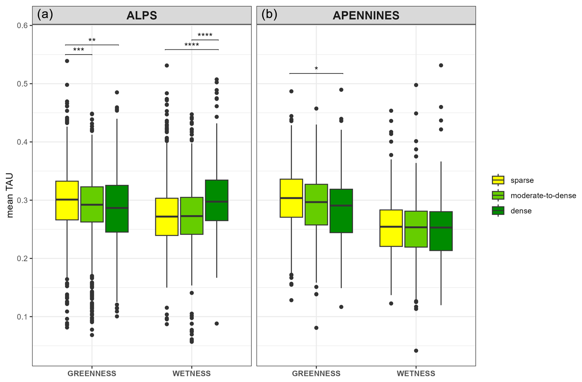
Figure 7 Boxplots of the mean TAU values of wetness and greenness trends in the Alps (a) and in the Apennines (b). The mean values in each forestline buffer account for three different canopy cover classes: sparse (yellow), moderate to dense (green), and dense (dark green). Significant differences between Wilcoxon tests are indicated with ^* (α≤0.05), ${}^{**}$ (α≤0.01), ${}^{***}$ (α≤0.001), and ${}^{****}$ (α≤0.0001). For more information on the canopy cover classes percentage in the Alps and in the Apennines, refer to Fig. B1 (Appendix B).

GAMs did not detect a statistically significant relationship between the greenness/wetness mean TAU values, the distance to forestline, and the elevation (Fig. 8). This result is probably due to the fact that a combination of topographic, climatic, and anthropogenic drivers must be considered to assess what are the main drivers of these spectral trends, taking into account the main differences between the Alps and the Apennines. Relatively similar patterns of the two index mean trends appeared at both mountain ranges but had a higher variability in the Apennines. In general, TAU greenness values were higher than wetness ones. In the Alps, greenness increased moving upward to the forestline with a first culmination close to and below it followed by a decrease and another increase, with the highest mean values being over 200 m. In the Apennines instead, the mean TAU values increased close to the forestline with a culmination above it (about 100 m distance) and were followed by a decrease, with the lowest values being above 200 m. In both mountain ranges, we observed a decrease in the greenness trends from lower elevations up to about 1750 m a.s.l. in the Alps and 1500 m a.s.l. in the Apennines (Fig. 8b). Thereafter, the mean TAU values increase progressively in the Alps up to 2300 m a.s.l., but decrease slightly in the Apennines to around 1700 m a.s.l. to rise again up to the altitudinal limit.

The wetness trend related to the forestline distance is very flat in the Alps and relatively similar to that of the greenness, whereas in the Apennines, the trend is far more variable and increasing progressively from the forestline to 200 m above it (Fig. 8a). Wetness curves decrease for both Alps and Apennines from the lower elevations to about 1600 m a.s.l (Fig. 8b), with a more pronounced slope for the Apennines. Then they both rise up to about 2100 m a.s.l. with a steeper and fluctuating trend again in the Apennines.

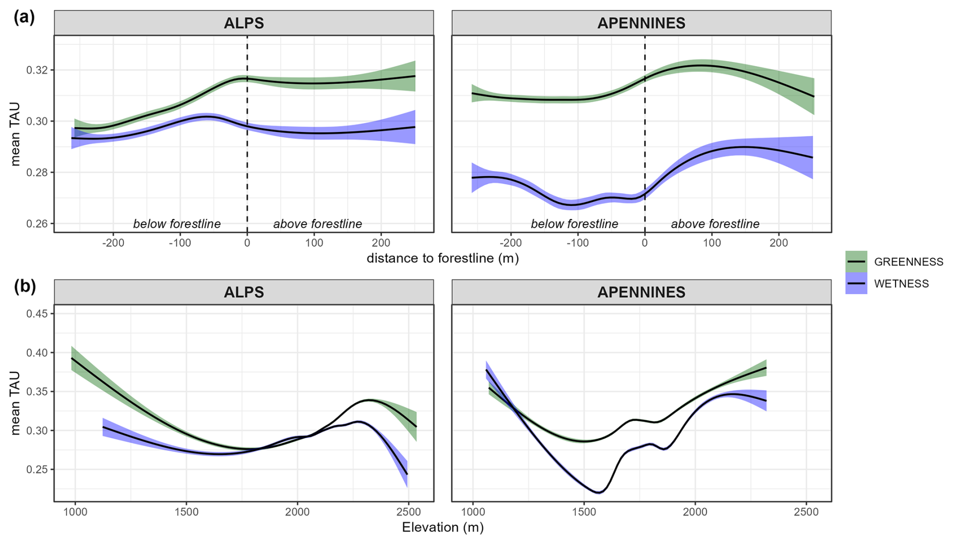
Figure 8 Wetness (blue) and greenness (green) GAM functions with a level of confidence of 0.95, according to the elevation (a) and to the distance to the forestline (b) in the Alps (left) and in the Apennines (right). We considered the mean values of each forestline buffer. The models are not statistically significant (α>0.05).

4 Discussions

4.1 The uppermost forestline detection method

The proposed forestline detection method is applicable at different spatial scales and in different geographic regions as it does not establish elevation thresholds and it can be based on regional datasets or other existing digital elevation models and forest masks. In addition, the method is also not exclusively based on climatic parameters; therefore, it is applicable for the detection of human-impacted forestlines. We considered forestlines closer to their potential climatic limit (e.g., tree species line), excluding forest margins at lower elevations and highly fragmented forestlines. We based the detection on the smallest elevation differences between the highest peaks and the forested pixels resulting from recent satellite-derived data (TCD). According to some authors, Italian and many other Northern Hemisphere forestlines could not be considered “climatic” treelines for their severe human constraints (e.g., grazing, fire, and deforestation) that altered altitudinal position, spatial patterns, and tree composition (Motta et al., 2006; Malanson et al., 2011; Piermattei et al., 2016; Vitali et al., 2018; Holtmeier and Broll, 2020). In Italian mountains, forest upward expansion was favored mainly by past large-scale disturbances and took place mainly at warmer aspects (Malandra et al., 2019). Recurrent human direct impacts on these ecotones since the Holocene times have greatly affected vegetation structure and composition (Foster et al., 1998), and recent silvo-pastoral abandonment at high-elevation sites triggered secondary succession (Debussche et al., 1999). The different forest cover and the bioclimatic features of the selected mountain groups provide a representative sample of the forestline trends along the Italian Peninsula. The mean forestline elevations detected confirm previous studies in the Alps (Caccianiga et al., 2008; Lingua et al., 2008; Diàz-Varela et al., 2010; Gilles et al., 2023) and in the Apennines (Vitali et al., 2018; Bonanomi et al., 2020). However, since the proposed method is closely dependent on the available regional/national datasets, some exclusion occurred with mountain groups at transnational borders.

4.2 Long-term greenness and wetness spectral trends

Overall, rising greenness and wetness trends were recorded at both mountain ranges in line with the ongoing natural reforestation processes (Vitali et al., 2018; Garbarino et al., 2020; Anselmetto et al., 2022). Pixel density distribution in the Alps and Apennines is globally very similar, but some differences occur for the dense canopy cover class in the Apennines, where the wetness indices have the highest trend peak just below the forestline. This could be attributed to the different species composition at the two mountain ranges. Along the Apennines, with the exception of some scattered locations with Pinus, Fagus sylvatica is practically the only upper-forestline species (Piermattei et al., 2014; Vitali et al., 2017). This would confirm the long-term impact of human activity (Körner, 2012) and explain the occurrence of “abrupt” (Harsch et al., 2011) and static treelines (Bonanomi et al., 2018; Bader et al., 2021) given the very limited seed dispersal efficiency of beech (Vitali et al., 2017). Dominant species colonization rates, reproduction, seed-dispersal strategy, and vitality of the occurring species are relevant issues when comparing forestlines shifts in the Alps and Apennines (Holtmeier, 2009; Compostella et al., 2017; Garbarino et al., 2020). In general, gap-filling processes prevail at the deciduous Apennine forestlines (Malandra et al., 2019; Vitali et al., 2018), whereas in the Alps the coniferous treeline species (e.g., Larix decidua, Pinus cembra and Picea abies) are more prone to tree encroachment at higher elevations. In the Apennine abrupt treelines, the beech regeneration (by seeds and suckers) have favored processes of canopy thickening and gap filling below and near the forestline, better intercepted by wetness indices that are more sensitive to the spectral response of the less exposed vegetation. Wetness indices are particularly sensitive to water content in both soil and plants especially in canopy leaf tissues. For this reason, we believe that significant increasing trends in areas with a dense canopy cover could be associated with crown thinning and biomass increase, as in gap filling, while in areas with sparse canopy cover, they could be associated with new encroachment in open areas.

Taking into account the magnitude of changes rather than their frequency, in the Apennines, we found a significant difference only for greenness mean TAU, lower in dense rather than in sparse canopy cover conditions. We assume that the drier climate of the Apennines may have influenced the positive trends of wetness indices, reducing the TAU variability in different canopy classes. The Wilcoxon test revealed the most significant variations in the Alps, where summer drought is not a limiting factor as in the Apennines. This hypothesis is confirmed by the higher mean TAU values of greenness in the sparse canopy class, whereas those of wetness refer to the dense one. Carlson et al. (2017) in the French Alps found a stronger greening signal in low shrubs and open areas (e.g., grasslands or rocky habitats) than in forested areas. As well McManus et al. (2012) in the forest–tundra ecotones in Canada found higher greening in shrub and grass canopy classes. Sometimes, the greening of sparse open areas may be affected by melting glaciers (Rumpf et al., 2022), inducing a possible increase in soil moisture and influencing wetness trends too. Without considering the canopy cover class, the most relevant changes in the Apennines occurred above the forestline and at the lowest (<1500 m a.s.l.) and highest (>2000 m a.s.l.) elevations. Further information about the forest structure could help detecting if the spectral signal sourced mostly from shrubs or newly established trees. In the Apennines, the highest mean TAU values above the forestline can be due to species such as Juniperus communis L., Pinus mugo Turra, and Vaccinum mirtillus L. that facilitate the upward migration of beech trees (Bonanomi et al., 2021). In the Alps, we found a steadier increase in TAU greenness and wetness from below to above the forestline. This confirms that diffuse treelines are more common in the Alps (Garbarino et al., 2020). Some authors used lidar data from the Global Ecosystem Dynamics Investigation (GEDI), integrated with Landsat and Sentinel-2 data (Potapov et al., 2021; Tolan et al., 2024; Lang et al., 2023) to assess canopy height, vertical canopy structure, and surface elevation with the aim of monitoring forest ecosystems and carbon fluxes. This approach could be adopted in monitoring ecotones such as treelines (Bolton et al., 2018) and also to predict future vegetation scenarios and provide suitable management options (Morales-Molino et al., 2022).

Considering the greenness and wetness mean values of TAU trends only as a function of elevation, without the forestline distance information, their higher values are mainly at lower sites, where temperature is less limiting and the past human impact was greater (Malandra et al., 2019; Anselmetto et al., 2022). Furthermore, forests at lower elevations are more accessible and usually have been most intensively managed in the past, although they now are largely abandoned (Malandra et al., 2019; Garbarino et al., 2020). Above the mean forestline elevation of both the Alps and Apennines, the mean TAU values increase and then decrease at higher altitudes where the number of pixels with significant increasing trends is also lower. In the Apennines, a second short but clear decrease above 1750 m a.s.l. may depend on the frequent abrupt beech treelines where the forest margin is sharply separated from areas with sparse and different vegetation. This common trend for both mountain ranges confirms an upward recolonization process at the Italian anthropogenic treelines. The decreasing magnitude observed at a higher elevation with the increasing distance from the forestline is probably due to the larger distance from seed trees (Vitali et al., 2018), the more limiting effect of temperature, and the synergic effect of topography and microclimate.

Uncertainty remains about what caused the spatial variability of trends, as noted also by Choler et al. (2021). The time series span and the spatial resolution of satellite images are crucial items in the definition of these ecological models. Nevertheless, the integration of different data sources (e.g., lidar) and the modeling of further environmental, climatic, and anthropogenic drivers can be useful for a better understanding of the current and future forestline dynamics.

5 Conclusions

This study proposes a novel method to demarcate at a regional scale the upper forestlines in geographic areas where the climatic treeline threshold (i.e., the 6 °C isotherm sensu Körner and Paulsen, 2004) can not be matched. We introduced several parameters to define only the forestlines closest to their potential position, detecting the ones nearest to mountain tops with land cover and bioclimatic features. The use of TCD, with national or European digital terrain models, makes this method applicable in most parts of Europe, but with similar datasets also in other world regions and at a different scale of analysis. High spatial resolution, wide geographical coverage, and open data availability policies are important issues for the replicability of the algorithm and for ensuring the quality of both the detection results and the trend analysis. Landsat images permit analyzing 40-year-long time series with a suitable spatial resolution. Even though the two types of indices have different targets (greenness indices for photosynthetic activity and wetness indices for water content), the results were congruous and emphasized the altitudinal expansion of the forestline ecotone at national scale. Wetness indices were more sensitive in areas with denser canopy cover, probably due to gap-filling processes and increasing biomass. Greenness indices detected more relevant trends, especially in areas with sparse or medium canopy cover, probably where recent tree encroachment occurred in previously open areas.

In the current context of climate change and post-abandonment successional dynamics, the implementation of semi-automatic methods for the detection and monitoring of vegetation spatial patterns and modeling of its spectral trends is definitely an added value. With this study, by different spectral indices, we detected hotspots of changes, and we put grounds for future landscape-scale analyses aimed at better assessing the relationships between climate, topography, vegetation dynamics, and forest structure changes.

Appendix A

Table A1 Selected Italian GMBA mountain groups, whose peaks having land cover and thermotypes suitable for the proposed algorithm. Elevation information was extracted from the Tinitaly DEM, limiting the areas to the national administrative boundaries.

Appendix B

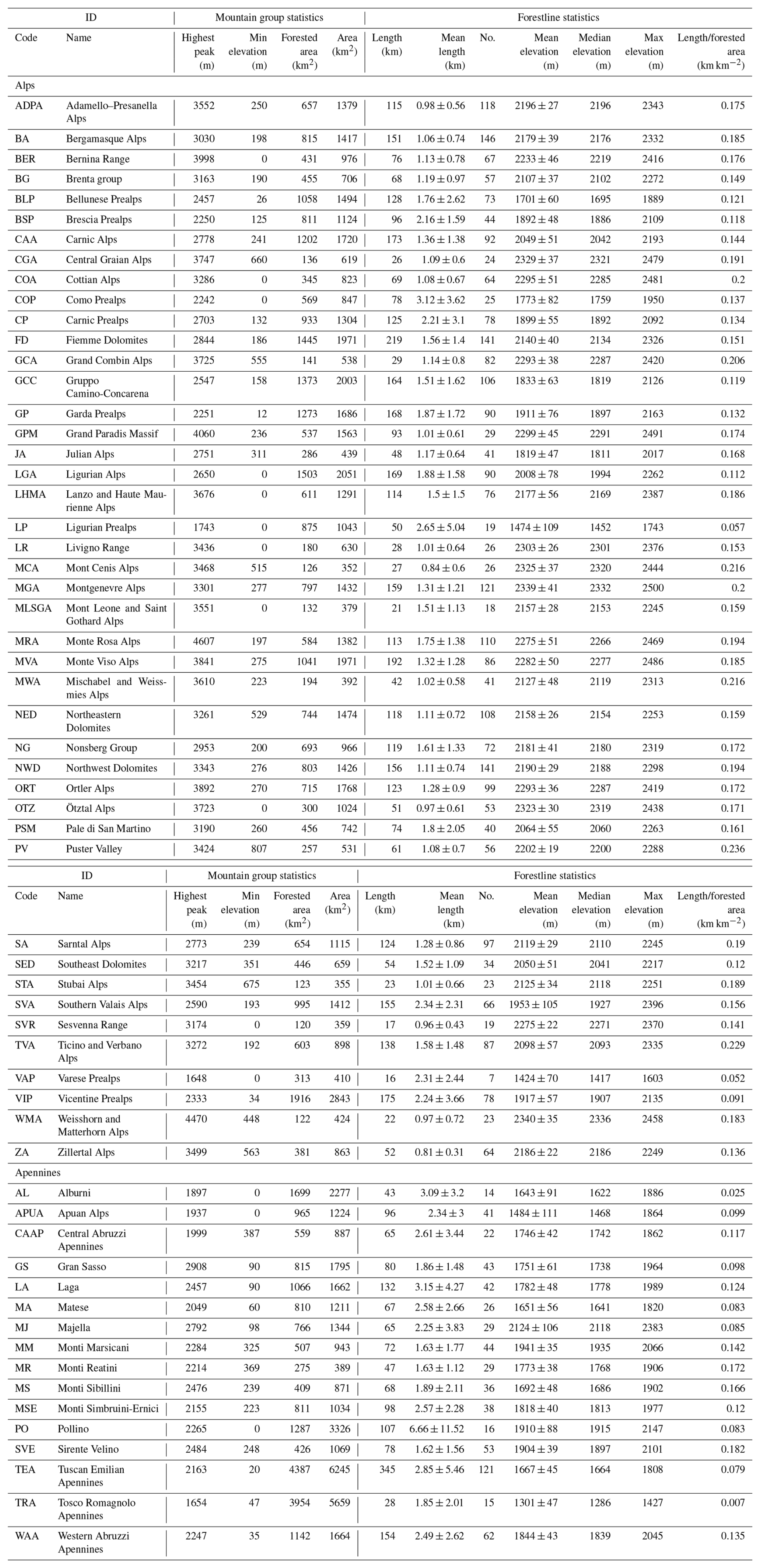
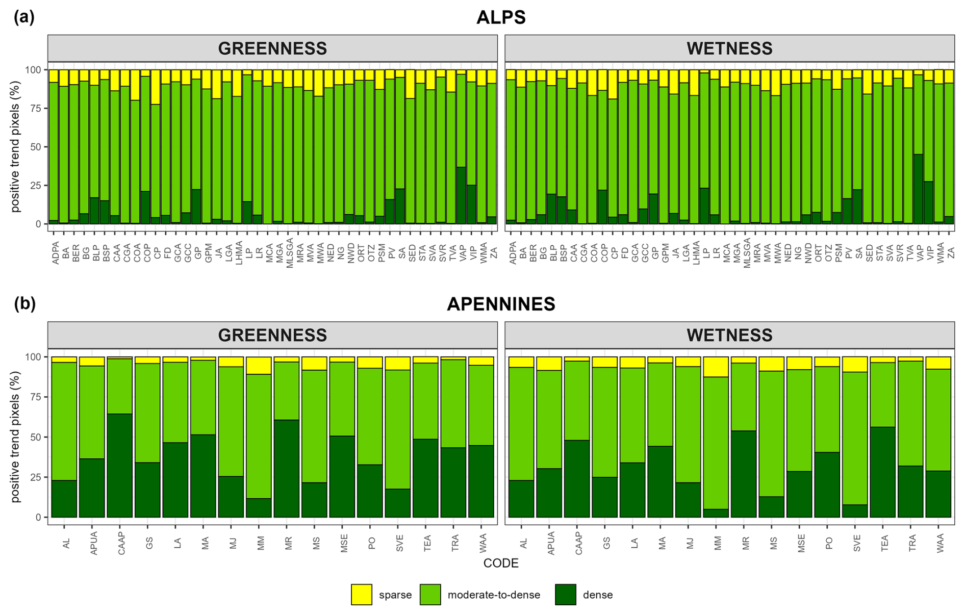
Figure B1 Percentage of highly significant positive greenness (left panels) and wetness (right panels) trend pixels of each tree cover density class in GMBA mountain groups of the Alps (a) and the Apennines (b). Code explanations are in Table A1 (Appendix A).