Grassland yield estimations – potentials and limitations of remote sensing in comparison to process-based modeling and field measurements

Grasslands make up the majority of agricultural land and provide fodder for livestock. Information on grassland yield is very limited, as fodder is directly used at farms. However, data on grassland yields would be needed to inform politics and stakeholders on grassland ecosystem services and interannual variations. Grassland yield patterns often vary on small scales in Germany, and estimations are further complicated by missing information on grassland management. Here, we compare three different approaches to estimate annual grassland yield for a study region in southern Germany. We apply (i) a novel approach based on a model derived from field samples, satellite data and mowing information (RS); (ii) the biogeochemical process-based model LandscapeDNDC (LDNDC); and (iii) a rule set approach based on field measurements and spatial information on grassland productivity (RVA) to derive grassland yields per parcel for the Ammer catchment area in 2019. All three approaches reach plausible results of annual yields of around 4–9 t ha⁻¹ and show overlapping as well as diverging spatial patterns. For example, direct comparisons show that higher yields were derived with LDNDC compared to RS and RVA, in particular related to the first cut and for grasslands mown only one or two times per year. The mowing frequency was found to be the most important influencing factor for grassland yields of all three approaches. There were no significant differences found in the effect of abiotic influencing factors, such as climate or elevation, on grassland yields derived from the different approaches. The potentials and limitations of the three approaches are analyzed and discussed in depth, such as the level of detail of required input data or the capability of regional and interannual yield estimations. For the first time, three different approaches to estimate grassland yields were compared in depth, resulting in new insights into their potentials and limitations. Grassland productivity maps provide the basis for the long-term analyses of climate and management impacts and comprehensive studies of the functions of grassland ecosystems.

1 Introduction

Grassland ecosystems provide fodder for livestock as well as many other ecosystem services, such as carbon storage, provision of habitat, water purification, recreation and erosion control (Bengtsson et al., 2019; Le Clec'h et al., 2019; Gibon, 2005, 2009; Richter et al., 2021; White et al., 2000). In Germany, grasslands cover almost one-third of the agriculturally used area (Statistisches Bundesamt, 2023) and are of central importance for the meat and dairy industry (Schoof et al., 2020b; Soussana and Lüscher, 2007). In large parts of Europe, grassland ecosystems are managed and, hence, strongly shaped by human activities. In Germany, for example, almost all of the grassland is under some form of agricultural use, i.e., grazed and/or mown with different frequencies (Dengler et al., 2014; Schoof et al., 2020a, c). Grassland management and use intensity, i.e., the number and timing of grazing and/or mowing as well as fertilization events, have a strong impact on grassland functions and ecology (Gossner et al., 2016; Neyret et al., 2021; Socher et al., 2012). Apart from climate and soil conditions, grassland management determines the productivity (and thus yields) and species diversity of these ecosystems (Gilhaus et al., 2017). In Germany, grasslands are managed on small units (parcels) individually, resulting in a wide variety of combinations of the number and timing of mowing events on small spatial scales. As a consequence, grassland landscapes can show high spatial and temporal variability in their biomass availability and species composition (Gerowitt et al., 2013).

Grassland biomass is usually directly used on farms as fodder for livestock and not traded, which is why there are usually no data on grassland yields resulting from sales statistics. The lack of information on yields exacerbates extensive spatiotemporal analyses of drivers of grassland productivity as well as modeling of grassland ecosystem services, e.g., nitrogen and carbon fluxes. Long-term effects of climate change and short-term weather extremes influence grassland productivity and yields (Beniston, 2003; Berauer et al., 2019). This is of particular importance in the Alpine and pre-Alpine regions of southern Germany, as the temperature in these areas increases twice as fast as the global average (Auer et al., 2007; Kiese et al., 2018). In addition, drought and heat episodes are expected to increase in the region. Therefore, information on grassland yields and the dependency on climate conditions is needed to support the planning of fodder production and imports for farmers and to inform administration and politics. Furthermore, information on grassland yields is required for a comprehensive assessment of grassland ecosystem services and sustainable management under changing climate conditions. Despite these information needs, continuous and large-scale monitoring is lacking.

There are different approaches to retrieve grassland yield information. Ground measurements alone, such as cutting and removing herbage from the grasslands for direct analysis or estimating yields by the use of a rising plate meter, are usually time-consuming processes, can hardly provide regular information and might not represent the conditions on broader spatial scales (Murphy et al., 2021). This holds in particular in grassland ecosystems characterized by a high small-scale variability, like in southern Germany. To retrieve spatially continuous and multi-temporal information, grassland yields can be (i) modeled empirically with a different degree of complexity, e.g.,  taking in situ and remote-sensing data into account; (ii) modeled bio-geochemically, e.g., with process-based models; or (iii) derived from simple rule sets used by authorities based on yield surveys and further spatially extensive data, e.g., elevation and soil fertility index.

Remotely sensed reflectance, in particular vegetation indices derived from them, depict vegetation greenness as well as structure and photosynthetic activity and, thus, relate to vegetation biomass (Holtgrave et al., 2020; Huete et al., 2002). Grassland traits, such as aboveground biomass, can be estimated using an empirical relationship employing remote-sensing and in situ data to train and validate models, as shown in many studies summarized in Reinermann et al. (2020). Space-borne remote-sensing-based biomass models have been applied in many different grassland ecosystems using various sensors and regression models. Using satellite remote-sensing data to quantify vegetation properties enables large-scale, continuous, reproducible and comparatively cost-sensitive monitoring. Compared with the relatively frequent application of empirical remote-sensing-data-based biomass models for mostly grazed grassland ecosystems (Wu et al., 2024; Yao and Ren, 2024), the number of studies using this approach for grasslands dominated by mowing is more limited (Reinermann et al., 2020). Previous studies from regions characterized by mown grasslands investigated the potential of various vegetation indices derived from medium-resolution sensors (the Moderate Resolution Imaging Spectroradiometer, MODIS, or the Moderate Resolution Imaging Spectrometer, MERIS) to estimate grassland biomass for single sites in Ireland and the Netherlands (Ali et al., 2017a; Ullah et al., 2012). Based on Landsat and Sentinel-2, grassland biomass and height were estimated for study regions in Germany, France, Spain and Austria using various regressors, such as multiple linear regression, random forest or deep learning models (Barrachina et al., 2015; Dusseux et al., 2022; Eder et al., 2023; Muro et al., 2022; Schwieder et al., 2020). However, despite the strong influence of grassland management on the productivity, to our knowledge, none of the previous remote-sensing-based studies have directly included mowing information in the biomass estimation approach. Further, grassland biomass estimates are only a snapshot in time. In particular for grasslands dominated by frequent mowing activities, the amount of standing biomass varies a lot over the course of a year. A single biomass estimation is, therefore, not sufficient to provide information on annual grassland productivity and yields. One way to approach this is the combination of multi-temporal biomass estimations informed by the timing of mowing events to retrieve annual grassland yields. To our knowledge, to date, there is no remote-sensing-based study that has estimated annual grassland yields using this approach.

Another method to obtain grassland yield estimates is the use of deterministic process-based models, such as LandscapeDNDC (Haas et al., 2013; Kraus et al., 2015; Petersen et al., 2021), Daycent (Del Grosso and Parton, 2019; Parton et al., 1998), PaSim (Riedo et al., 1998, 2000), LPJmL (Bondeau et al., 2007; Schaphoff et al., 2018), APSIM (Holzworth et al., 2014) or ORCHIDEE-GM (Chang et al., 2013). An advantage of process-based models is the possibility to assess all spatial levels, ranging from the site (Chang et al., 2013; Liebermann et al., 2020; Petersen et al., 2021) to the continental (Vuichard et al., 2007) and global (Rolinski et al., 2018) scale. Additionally, the application of process-based models opens the possibility to evaluate ecosystem productivity under various scenarios including climate change (Petersen et al., 2021) or management changes like adaptions in fertilization regimes (Hong et al., 2023; Reis Martins et al., 2024) or shifts in cutting frequencies (Rolinski et al., 2018). However, as process-based models rely on the availability of data for model development, the testing and, in particular, up-scaling of large-scale applications are limited.

A third approach to estimate grassland yield is by making use of measurements from field experiments or regional census statistics (Smit et al., 2008). In Germany, some federal states provide reference values for grassland yields at the county level that can be used by farmers to derive their grassland's fertilizer requirements. For instance, the reference values provided in the guideline for fertilization of crop- and grassland by the Bavarian State Institute for Agriculture (LfL) (LfL, 2018) are aggregated values for Bavaria based on LfL internal research and field experiments (Diepolder et al., 2016).

Here, a novel remote-sensing-based approach to derive grassland yield in southern Germany is presented and applied. Annual grassland yields are compared to yield estimates of the same year and region derived from two other approaches – either established in the scientific community or used by authorities – optimized for the study region. Annual yields are compared, and the advantages and disadvantages of the approaches are highlighted. We estimate annual grassland yields for a study area in southern Germany in 2019 using (a) a novel empirical satellite remote-sensing (RS) model, which is compared with results of (b) a process-based biogeochemical model (LandscapeDNDC) and with (c) a simple rule set reference value approach used by authorities (RVA). To represent grassland management intensity, all three approaches use information on satellite-derived mowing dates retrieved from Reinermann et al. (2023, 2022). To examine the conditions under which the results of the three various approaches differ, we examined the influence of various factors – management and climate – on the grassland yields resulting from the three methods. By examining the spatial and temporal patterns of yields derived from the three approaches and analyzing the influence of various factors, we assess the differences and similarities in the methods. We aim to determine which method best represents specific conditions and under which circumstances it is most reliable.

2 Study area

The study area is located in the pre-Alpine and Alpine region of southern Germany (Fig. 1) and consists of the broader Ammer catchment area including the TERENO Pre-Alpine Observatory (Kiese et al., 2018). The area belongs to the temperate oceanic climate according to Köppen and Geiger (Kottek et al., 2006). The mean annual temperature was 8.9 °C in 2019, and the long-term average (2012–2021) was 8.1 °C for the region. The mean precipitation sum was 1175 mm in 2019, and the long-term average was 1141 mm for the area (Boos et al., 2024; Petersen et al., 2021). The elevation of the study area with grassland land use ranges between 500 and 1100 m above sea level (m a.s.l.), with grasslands dominating agricultural land use, which totals to about 38 % of the region area (Kiese et al., 2018). In the region, grasslands are of economic importance not only for meat and dairy production but also for tourism (Schmitt et al., 2024; Soussana and Lüscher, 2007). The grasslands of the Ammer region are grazed and/or mown at intensities ranging from extensive (with one to two mowing events) to highly intensive (with up to six mowing events per year) use (Reinermann et al., 2022, 2023). The timing of the management activities varies from grassland parcel to parcel. Here, we focus on meadows and mowed pastures, which make up around 657 km² (27 138 parcels).

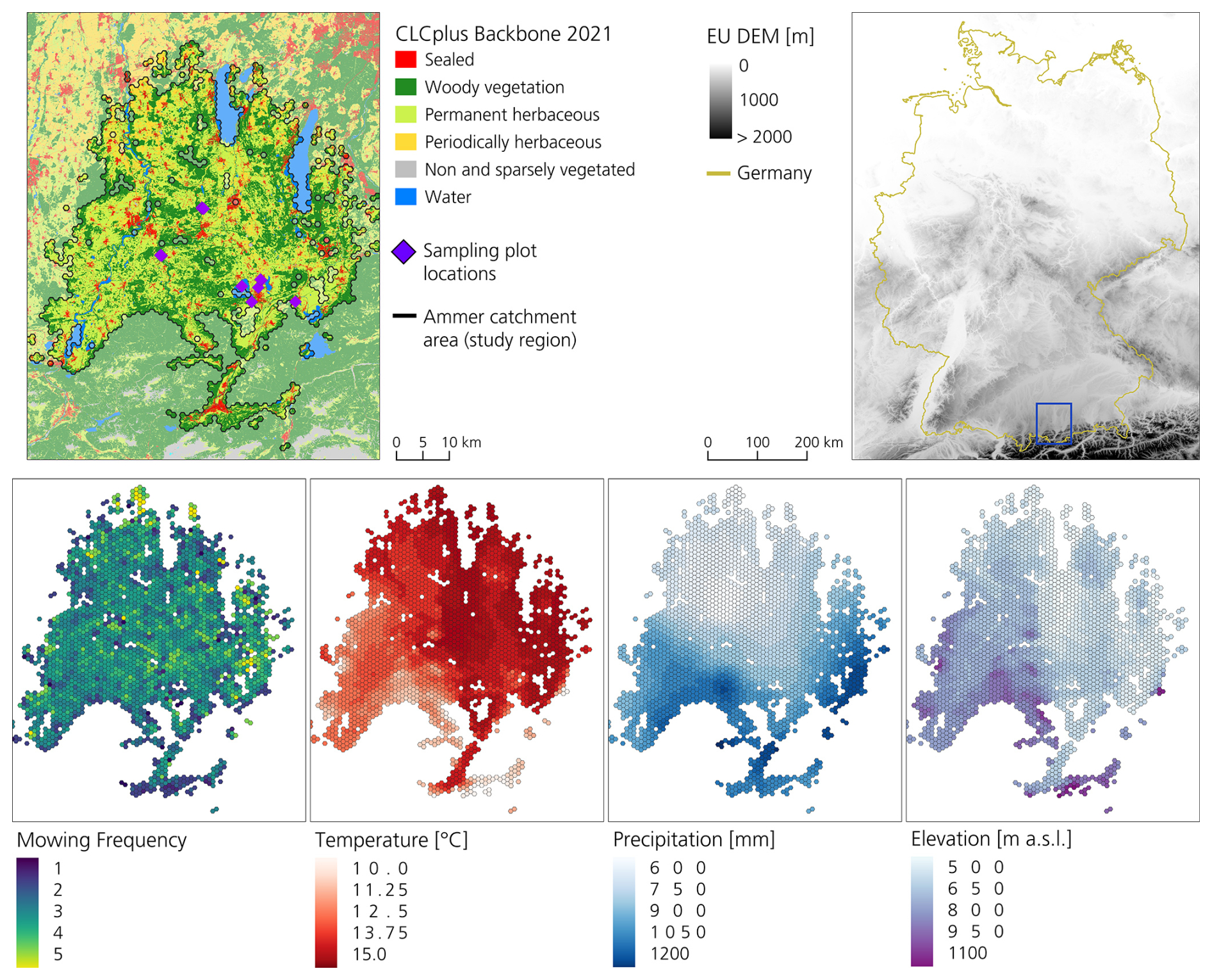
Figure 1 The top row presents maps of study area in southern Germany showing land use and elevation. The bottom row shows the hexagon averages of the mowing frequency, mean annual air temperature, mean annual precipitation and elevation for the year 2019 (see Sect. 3.2.2). The hexagon diagonal size is 1 km.

3 Material and methods

3.1 Spatial and field data

3.1.1 Spatial management data

All three yield modeling approaches used the same parcel boundary and mowing information data. Parcel boundaries were taken from the EU's Integrated Administration and Control System (IACS) provided by the LfL. The same data source was used to exclude all parcels that were not used as meadows or mowing pastures in 2019.

The dates of mowing events originate from Reinermann et al. (2023, 2022), where mowing events were detected based on Sentinel-2 time series. However, differing from the original approach, no grassland mask was used for this study to ensure that all meadows and mowed pastures identified by the IACS data were covered. To transfer the 10 m×10 m pixel-based mowing dates to the parcel level, detected dates within a time frame of 3 weeks were agglomerated per parcel using the majority vote. Only when the date was detected for 20 % of the parcel did the mowing event remain in the dataset. Regional validation using information from farmers and webcam images showed an accuracy (F1 score) of 0.65 for the mowing dates at the parcel level in the Ammer region in 2019. The validation was conducted only with data from the study region but in the same manner as in Reinermann et al. (2022).

3.1.2 Biomass field data

In situ biomass measurements were used to train and validate the empirical remote-sensing model and for regional quality evaluation of LandscapeDNDC. A total of 14 grassland plots of 20 m×20 m in the Ammer region (Fig. 1) were sampled in the 2019–2021 period to obtain in situ aboveground biomass (AGB) information (Schucknecht et al., 2023, 2020). The sampling plots comprised homogeneous vegetation coverage and were placed to be representative of the entire grassland parcel. The sampled grassland parcels were characterized by different land management intensities ranging from one to six mowing events per year. The sampling campaigns took place at multiple times during the growing season to ensure that biomass samples from a variety of growth stages before and after mowing events were included. For each plot, aboveground biomass was collected on four randomly placed 50 cm×50 cm subplots. The plot was divided into four equal quadrants, with each subplot being randomly positioned in one of the quadrants. The position of each subplot varied with every measurement. To account for mowing height, AGB was sampled from >7 cm on all subplots and complemented by one biomass sampling from 2 to 7 cm vegetation height at one of the four subplots. The samples were dried at 60 °C for at least 48 h until constant weight and then weighed. The weight values of the dried biomass of the four samples from above 7 cm were averaged, added to the measurements of 2–7 cm to obtain the total AGB per site and date, and scaled to 1 m². In total, 111 biomass samples were collected. Apart from three grassland plots that were used as alternatives when the actual plots were freshly mown at the time of the campaign, all plots were sampled five times in 2019, three times in 2020, and once in 2021 between March and October. Among the 14 grassland plots, one was mown six times, two were mown five times, four were mown four times, three were mown three times, one was mown two times and three were mown only once per year.

3.2 Yield estimation approaches

The three grassland yield estimation approaches applied in this study, i.e., the remote-sensing (RS) approach, the process-based LandscapeDNDC model approach (LDNDC) and an estimation based on reference values (RVA), are described in detail in Sects. 3.2.1–3.2.3 (Fig. 2).

Figure 2 Conceptual scheme of the three yield estimation approaches.

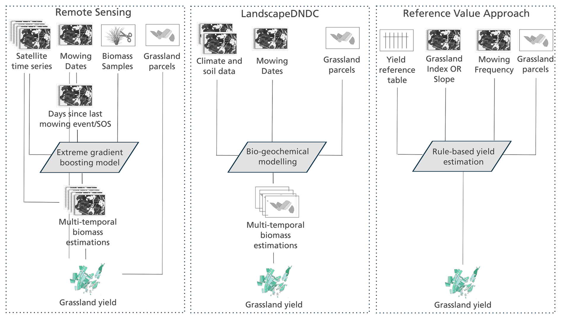
3.2.1 Remote-sensing-based approach

For the remote-sensing model, MAJA (version 3.3) Sentinel-2 (S2) level 2a (Hagolle et al., 2017) time series from the years 2019–2021 and tiles 32TPT and 32UPU were used to match the biomass sampling campaigns. The optical satellite reflectance data consist of acquisitions from two identical satellites (S2A and S2B) acquiring information in 12 spectral bands (Drusch et al., 2012). The bands used here are the 10 bands relevant for vegetation monitoring, namely, bands 2, 3, 4, 5, 6, 7, 8, 8A, 11 and 12, covering the red, green, vegetation red-edge, near-infrared and shortwave-infrared wavelengths. The bands that have a 20 m spatial resolution were resampled to 10 m by the nearest-neighbor method to achieve a consistent spatial resolution of 10 m for all bands.

Based on S2 satellite data and in situ total AGB samples (Sect. 3.1.2), an empirical model was trained and optimized to estimate grassland biomass. Satellite data influenced by clouds, cloud shadows or unfavorable terrain conditions were excluded according to the MAJA algorithm. The empirical model was built based on the S2 reflectances from the 10 selected bands and additional spectral indices as predictor variables. Specifically, the enhanced vegetation index (EVI, Eq. 1; Huete et al., 2002) and the tasseled cap wetness index (Wetness, Eq. 2; Indexdatabase, 2024; Krauth and Thomas, 1976) were calculated and included as they relate to vegetation biomass:

$$\begin{array}{}\text{(1)}& {\displaystyle }& {\displaystyle }\text{EVI}=\mathrm{2.5}{\displaystyle \frac{\text{B8}-\text{B4}}{\text{B8}+\mathrm{6}\cdot \text{B4}-\mathrm{7.5}\cdot \text{B2}+\mathrm{1}}},\text{(2)}& {\displaystyle }& {\displaystyle }\begin{array}{rl}{\displaystyle }\text{Wetness}=& {\displaystyle }\mathrm{0.1509}\cdot \text{B2}+\mathrm{0.1973}\cdot \text{B3}+\mathrm{0.3279}\cdot \text{B4}\\ {\displaystyle }& {\displaystyle }+\mathrm{0.3406}\cdot \text{B8}-\mathrm{0.7112}\cdot \text{B11}\\ {\displaystyle }& {\displaystyle }-\mathrm{0.4572}\cdot \text{B12},\end{array}\end{array}$$

where B2, B3, B4, B8 and B11 are reflectance bands in the blue, green, red, near-infrared and shortwave infrared areas, respectively.

In addition, information on the timing of mowing events (Sect. 3.1.1) was directly included in the modeling process by adding an additional predictor variable representing the days since the last mowing event. For each S2 acquisition, a layer was calculated giving the days since the last mowing event on a pixel basis. When no mowing event took place before the S2 acquisition, the number of days since the start of the growing season was calculated. To retrieve the start of the growing season, the Copernicus Land Monitoring Service (CLMS) High Resolution Vegetation Phenology and Productivity (HR-VPP) Start of Season product was used (CLMS, 2019). Further, the S2 acquisition date was included as a predictor variable. This resulted in 14 input features for the empirical modeling, i.e., 10 spectral bands, 2 spectral indices, the number of days since last mowing or start of growing season, and the date of the satellite acquisition.

To prepare the input data for model training, pairs of cloud-free S2 acquisitions and corresponding in situ biomass samples were built by allowing a maximum of 5 d between a satellite acquisition and field sampling in both directions. If there were multiple satellite acquisitions in the allowed range, closer acquisitions and acquisitions after field sampling dates were preferred. It was also checked that there was no mowing event in between a satellite acquisition and a field sampling date to maintain representative data pairs. Due to cloud conditions in 2021, only data from 2019 and 2020 remained in the data table after this procedure. Data pairs from sampling campaigns from every month between April and October, apart from July and August, were available.

An extreme gradient boosting model was trained on the input features and the corresponding AGB values (Friedman, 2001). Initial tests showed that the extreme gradient boosting model outperformed others, such as random forest, support vector machines or multiple linear models. The XGBoost package (version 1.5.2) was used in Python. In total, 74 data pairs were available, from which 82 % (n=61) of data pairs were used for training and testing, while 18 % (n=13) of data pairs were used as an independent test of the trained model. A stratified sampling of the test data was conducted to ensure that the value range of the test data was representative. With the data used for training, the hyperparameters for an optimized model were searched for, using grid search, 5-fold cross-validation (CV) and 10 iterations each. To find the best model, the coefficient of determination (R²) was used. The best model according to the training was then tested against the independent test dataset.

The best-trained biomass model was applied to estimate the AGB of all available S2 scenes to generate a biomass time series. This biomass time series was used in combination with the mowing dates and IACS parcel information to estimate annual yields per parcel. This was approached by going through the parcel-based mowing dates. For each mowing date, the pixel-based biomass estimates from all observations of up to 3 weeks before and 1 week after the mowing date were extracted. The 95th percentile was calculated from this biomass data to estimate the yield per mowing event and parcel, minimizing the influence of parcel boundaries. This time frame was used to ensure that the biomass was captured shortly before a mowing event, as there is an uncertainty in the timing of the mowing dates. These single-mowing-event yields were then summed up to calculate the annual yields per parcel.

3.2.2 LandscapeDNDC modeling approach

The process-based biogeochemical model LDNDC was run for the whole study region with individual high-quality input data combinations of soil, climate and management for every field (Boos et al., 2024). This was made possible by the availability of (1) accurate small-scale grassland soil profile data, (2) interpolated reference climate data based on continuous measurements from weather stations and (3) cutting dates from remote sensing at the field level.

The model calibration and validation for yields was performed on extensive lysimeter measurements from the TERENO Pre-Alpine Observatory covering three sites at different elevations within the study area with intensive and extensive management (Kiese et al., 2018; Petersen et al., 2021). Running the model with regional input data for the sites, which are used for RS training and validation (see Sect. 3.1.2), and comparing to standing biomass before cutting events lead to a coefficient of determination of 0.67 and a root-mean-square error (RMSE) of 1.46 $\mathrm{t}{\mathrm{ha}}^{-\mathrm{1}}{\mathrm{a}}^{-\mathrm{1}}$ (Boos et al., 2024).

Climate inputs were generated from the reference data of the ClimEx project (Poschlod et al., 2020; Willkofer et al., 2020) – interpolated from station measurements of the German Weather Service – which we aggregated to daily climate inputs (minimum, maximum and mean air temperature; precipitation sum; mean relative humidity; mean global radiation; and mean wind speed) and assigned the nearest virtual climate station to every field to run LDNDC. Regional soil data were derived from the soil database of the LfU (LfU, 2020). Only mineral grassland soils were considered, and a unique, i.e., with a single profile per polygon, soil map was compiled. More details can be found in Boos et al. (2024).

The model simulates plant growth depending on factors like photosynthesis, nitrogen and water availability, phenology, and temperature (Petersen et al., 2021). At a prescribed cutting date, the aboveground biomass is reduced to a preset value for the remaining biomass, which equals the standing biomass after the cutting event and is assigned according to the farmers' practice calibrated to a cutting height of about 7 cm. The harvested biomass from all events in a year is then summed to calculate the annual yield per field. Therefore, management is another key model driver and was set for every parcel individually. The cutting dates in the study year 2019 were taken from the dataset generated by Reinermann et al. (2022), as described in Sect. 3.1.1. Fertilizer, in the form of slurry, was applied according to the mowing information following the farmers' practice in the study region. For parcels with three or more mowing events per year, the number of manuring events equalled the number of cuts. For parcels with less than three mowing events per year, the number of fertilizer applications was one less than the number of cuts, which corresponds to local farmers' practices. The amount of manure varied between 40 and 55 kg N ha⁻¹ per event and decreased per application. For further details on the applied regional model drivers for LDNDC, see Boos et al. (2024).

For every grassland field simulation (N=27 138), climate, soil and management input were derived from superimposing field boundaries with the respective spatial products. The model (LDNDC revision: 10786; crabmeat revision: 8136) was run with an hourly time step with the following submodels: CanopyECM (Grote et al., 2009) as the microclimate module; WatercycleDNDC (Kiese et al., 2011) as the water cycle module; MeTrx (Kraus et al., 2015) as the soil chemistry module; and PlaMox (Kraus et al., 2016; Liebermann et al., 2020), employing the PhotoFarquhar model (Ball et al., 1987; Farquhar et al., 1980) for photosynthesis, as the physiology module. For a general description of LDNDC and the functioning and interaction of the different submodules, see Petersen et al. (2021).

3.2.3 Reference values approach

The reference values approach (RVA) is mainly based on a look-up table from the LfL that includes yield reference values of the farmers' yield for Bavaria for (i) different types of grassland uses and intensities (number of cutting events, low/medium/high grazing intensity) as well as yield levels (low/medium/high) (see Table A1). Apart from the mowing information (Sect. 3.1.1), cattle numbers (Sect. 3.1.1) were used to identify the management intensity (i). We further used the land appraisal dataset (LDBV, 2018) to obtain grassland indices (German “Grünlandzahl”) for each field to get the yield levels (ii). This index represents the quality of a location for grassland production, considering factors such as soil type, soil properties, climate and water availability. The index ranges from 1 (poor) to 100 (best). As the grassland index can vary within a parcel, we assigned the value that covered the largest portion of the parcel area. In cases where the grassland index was unavailable, we substituted it with the field's maximum slope (ASTER GDEM, 2018) instead. The assumption was that the management intensity and, consequently, the grassland yields decrease with increasing slope. The management intensity dataset described in Sect. 3.1.1 was used to allocate the number of cutting events to each grassland field. For mowed pastures, the share between mowing and grazing first had to be identified in order to determine their use intensities. Mowed pastures with one cutting event were defined as having 60 % grazing use, while all mowed pastures with at least two cutting events were defined as having 20 % grazing use. Second, the management intensity of mowed pastures was approximated by the farm's stocking rate (SR) for all parcels with zero to three cuts; i.e., the higher the SR, the higher the use intensity. SR is defined as LSU per P, with LSU being the number of cattle per farm in livestock units and P being the farm's total grazing area. Mowed pastures with more than three cuts were assumed to have a high use intensity (Table A2). All assumptions regarding the slope, share of grazing in mowed pastures and SR were discussed with and approved by scientific grassland experts and experts from the Office of Food, Agriculture and Forestry (AELF) Weilheim, Germany – a local stakeholder from the study region. More information can be found in Kaim et al. (2025).

3.3 Spatial aggregation of yield data and comparisons

The annual yields estimated by all three approaches are compared for any individual parcel (N=27 138 meadows and mowed pastures) as well as for mean values of hexagons (1 km diagonal), with a total of 2571 hexagons covering the full study region. The yields were averaged per hexagon by weighting them by the parcel areas. The aggregation on hexagons is done for several reasons: firstly, the publication of the parcel shapes and locations is not permitted due to data privacy regulations; secondly, the visibility of spatial patterns is improved; and, lastly, outlier effects are minimized.

To compare the yields per parcel and hexagon resulting from the three different approaches, the Pearson correlation coefficient was calculated. To analyze the effect of influencing factors, the relationships between yields and mowing frequency, temperature, precipitation and elevation were plotted, and the Pearson correlation coefficients were calculated.

4 Results

4.1 Grassland biomass estimation

4.1.1 Biomass estimation based on the RS approach

Sub-parcel biomass estimations are intermediate products of the RS approach. Figure 3 shows the estimated biomass for single satellite observations at the pixel resolution (10 m×10 m), highlighting the potential to capture small-scale variability in patterns of standing biomass and grassland productivity using the RS approach.

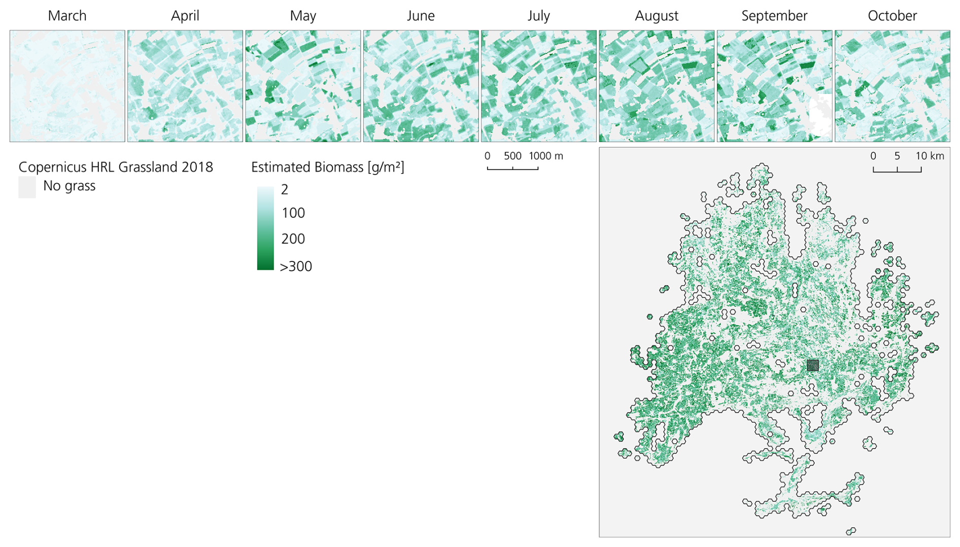
Figure 3 Estimated grassland biomass using the RS approach for single time steps (30 March, 19 April, 24 May, 13 June, 23 July, 27 August, 16 September and 16 October) and annual mean biomass for the entire study region with a 10 m×10 m pixel resolution. The top panel location is indicated as a square in the map of the whole study region.

The estimated biomass values from RS were validated with the part (18 %) of the in situ measurements that were not used for model training (i.e., the test data). The best RS model – extreme gradient boosting regressor, parameterized with a learning rate of 0.05, a maximum depth of each tree of three and a number of features used in each tree of 40 % – reached an average R² (CV) of 0.97 and a RMSE (CV) of 0.18 t ha⁻¹ during the internal validation. Band 12 (shortwave infrared), wetness index and days since the last mowing were the most important features according to the relative influence measure. The validation of the model with the test dataset (n=13) lead to an R² value of 0.68 and a RMSE of 0.43 t ha⁻¹ (see Fig. 4).

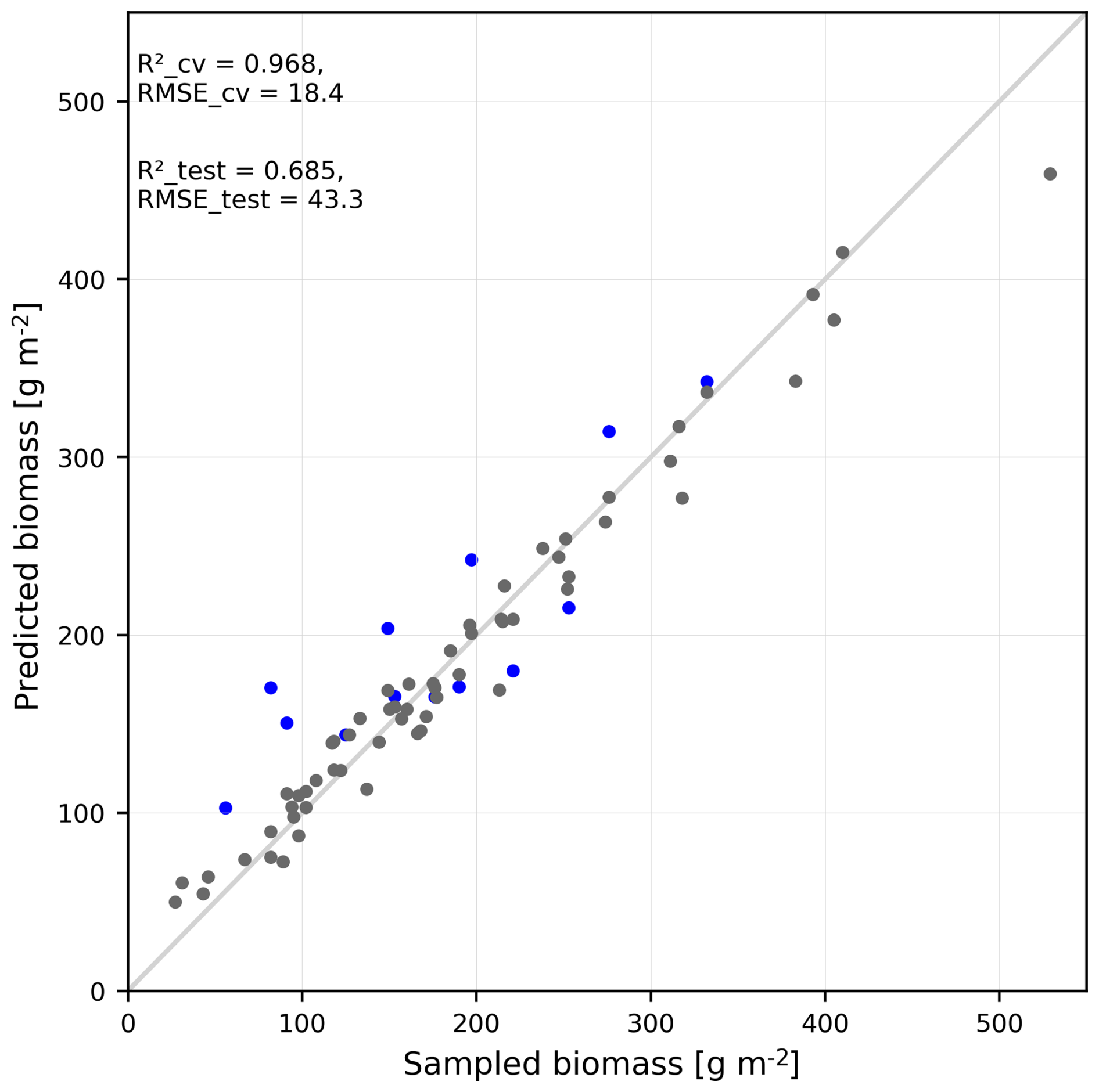
Figure 4 Predicted against sampled biomass (AGB; g m⁻²) for cross-validation and test data using the RS approach.

4.1.2 Comparison of RS and LDNDC biomass estimations

Time series of AGB for the year 2019 for three example parcels from the measurement campaign that were used for the RS biomass model training and validation (Sect. 3.1.2) are illustrated in Fig. 5. The figure includes the AGB of in situ measurements, estimated AGB derived by the RS and LDNDC approaches (not available for RVA), and the annual yield based on all three estimation methods. The temporal pattern of LDNDC biomass estimations shows an increase in spring, a drop after mowing and an increase thereafter. The LDNDC biomass at the first cut is the highest. The temporal profile of the RS-based biomass follows the mowing dates less strictly compared with LDNDC; however, for most mowing events, there is a peak before the mowing event, followed by a drop and a regrowth pattern (Fig. 5). When comparing the two biomass time series it becomes clear that the yield of the first mowing event from LDNDC is notably higher than from RS. In contrast, at times, RS shows a gradual decline in the local maxima during the growing season (e.g., Fig. 5, top panel).

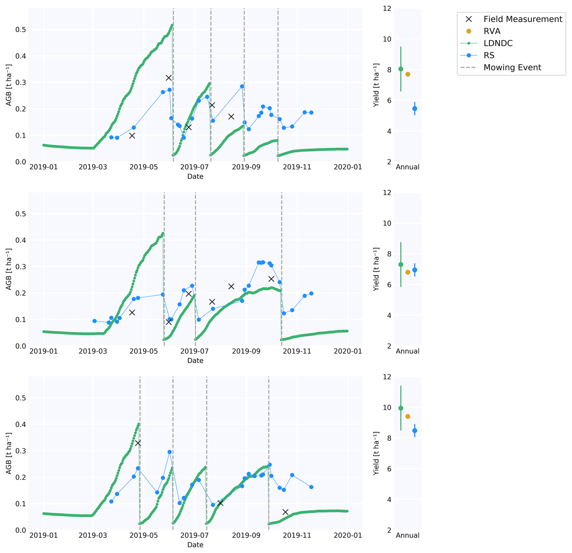
Figure 5 Temporal patterns in grassland AGB estimated by the RS and LDNDC models, in situ measurements of AGB, annual yields of all three models (on the right of each subfigure), and mowing dates (vertical dashed lines) of three grassland parcels in the study area.

The LDNDC model and the regional input data have also been evaluated against the AGB measurements/in situ data of the abovementioned field campaign (Sect. 2.2.2) in a previous study (Boos et al., 2024). To this end, only biomass measurements from within 1 week before a mowing event were considered and summed to yearly values per parcel. With this procedure, an R² value of 0.67 and a RMSE value of 1.46 $\mathrm{t}{\mathrm{ha}}^{-\mathrm{1}}{\mathrm{a}}^{-\mathrm{1}}$ were found.

4.2 Estimated annual grassland yields

The spatial patterns of the annual grassland yield averaged per hexagon estimated with each method are depicted in Fig. 6. All three models achieve plausible results, with respect to annual grassland yields ranging mostly between 3 and 9 t ha⁻¹ for the Ammer region in 2019. The average annual grassland yields of the entire study region estimated by the three models are as follows: 6.5 t ha⁻¹ (372.9 kt) for RS, 7.4 t ha⁻¹ (445.5 kt) for LDNDC and 6.9 t ha⁻¹ (419 kt) for RVA. The yield maps highlight the spatial variability in grassland yields in the study region, which is consistent in many cases for the three modeling approaches. Noticeable patterns are grasslands with relatively high annual yields in the north of the study region according to the RS and LDNDC models and, to a lesser degree, according to the RVA. Grasslands with lower annual yields are present in the northeastern and the eastern parts of the study area, as is mostly visible in the RS and RVA maps. The center of the study area shows grasslands with above-average yields mostly based on the RS and, even more so, the LDNDC model results. Grasslands in the southern part of the study area located within Alpine valleys show lower yields, in particular for the RS and RVA maps. The entire southwestern part of the region shows overall lower grassland yields from the RS and LDNDC models but not the RVA model (Fig. 6).

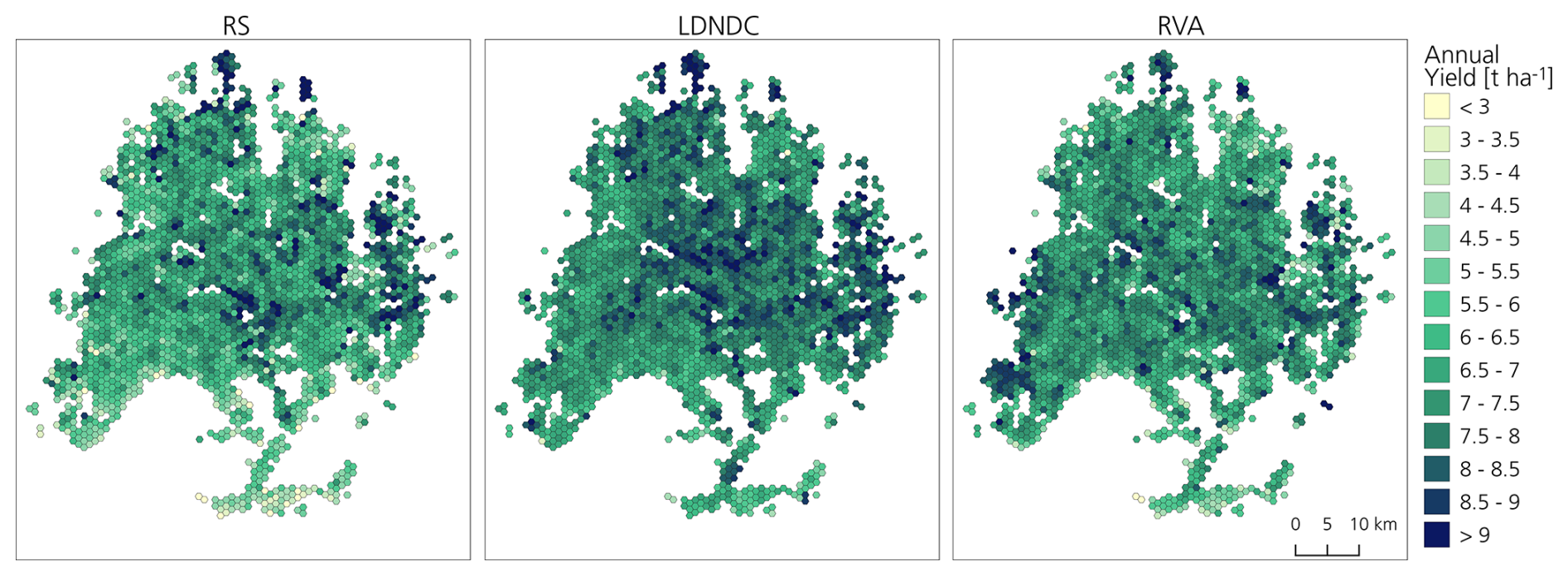
Figure 6 Spatially aggregated (hexagon diagonal length of 1 km) annual yield estimates for meadows and mowed pastures in the study area in 2019 based on remote sensing, LandscapeDNDC simulations and the reference values approach. Hexagons for which the grassland area is smaller than 1 ha are not shown.

The differences in yields based on RS and LDNDC are not concentrated in specific locations; rather, they are distributed throughout the Ammer region (Fig. 7). In both cases, the yield differences of RS and LDNDC with RVA show a northeast–southwest pattern, as yields derived from RVA are higher in the southwestern part of the study region compared with yields based on RS and LDNDC. Direct comparisons of hexagon yields reveal that 36 % of the Ammer region shows differences smaller than 1 t ha⁻¹ among all three approaches. The standard deviation of yield averages of all three methods shows no distinctive spatial patterns (see Fig. A2).

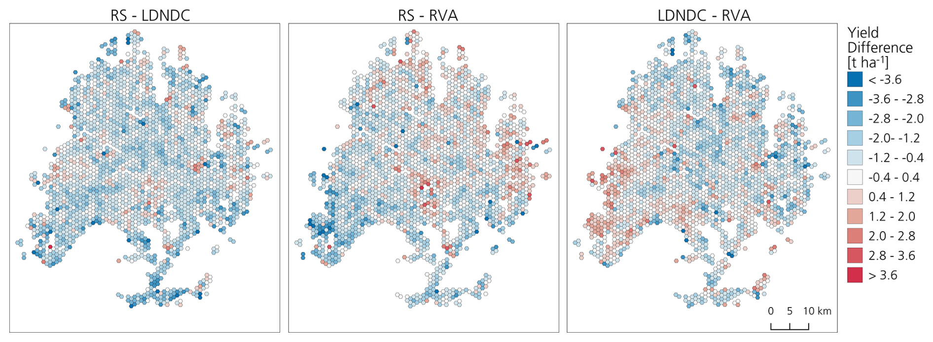
Figure 7 Differences between spatially aggregated (hexagon diagonal length of 1 km) annual yield estimates for meadows and mowed pastures in the study area in 2019 based on remote sensing, LandscapeDNDC simulations and the reference values approach. Hexagons for which the grassland area is smaller than 1 ha are not shown.

In order to compare the estimated annual grassland yields averaged per hexagon for the three approaches, the frequency distributions were plotted along with the correlation of the annual yield estimates from the different approaches (Fig. 8). The frequency distribution shows the largest range for the RS method (variance of 2.0 compared to 0.9 for LDNDC and 1.2 for RVA). The peaks showing the highest estimated yields are around 7 t ha⁻¹ for RS and around 7.8 t ha⁻¹ for LDNDC and RVA. The comparison of the hexagon yields of the RS and LDNDC approaches shows that they largely overlap, in particular for the most common yield values of 6–8 t ha⁻¹. The Pearson correlation coefficient is 0.67 for the hexagon yields based on RS and LDNDC. It shows significant relationships in all combinations of methods. In general, although particularly for yields below approximately 5 t ha⁻¹, LDNDC shows higher values compared to the RS (and RVA) results. The comparison of annual yields averaged per hexagon from the RS and RVA models also show generally good agreement (Pearson's r=0.64) but an overall larger scattering. The hexagon yields of RVA compare well with the RS yields and also show a tendency toward over- or underestimation, respectively, for smaller value ranges below approximately 6 t ha⁻¹ when compared to LDNDC yields (Fig. 8). The relationship between RVA and LDNDC yields is the weakest, with a Pearson r value of 0.47.

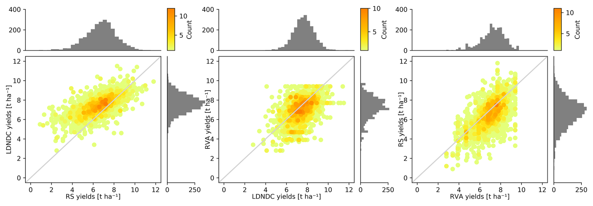
Figure 8 Pairwise relationships of spatially aggregated (hexagon diagonal length of 1 km) annual yield estimates for meadows and mowed pastures in the study area in 2019 based on remote sensing, LandscapeDNDC simulations and the reference values approach with histograms of the three modeling approaches.

The frequency distributions and pairwise comparisons of the estimated annual grassland yields per single parcel are shown in Fig. A1. The higher spatial resolution leads to increased scattering for all three approaches compared to the hexagon averages. The yields derived from RS show a variance of 4.6, a 95th percentile of 9.7 % and a 5th percentile of 2.5 t ha⁻¹. LDNDC and RVA yields have a variance of 2.2 and 2.7, a 95th percentile of 9.8 and 9.4, and a 5th percentile of 4.9 and 3.9 t ha⁻¹, respectively. The RVA method results in discrete values, in contrast to the other two approaches, and does not predict values higher than 10 t ha⁻¹. Due to the discrete values of RVA, there is a much higher overlap of yield values, resulting in higher counts for the relationships including RVA and varying count scales in Fig. A1. The relationships between the estimated yield based on the three approaches are relatively similar to those for the hexagon means, with a Pearson r value of 0.64 between RS and LDNDC, 0.54 between RS and RVA, and 0.44 between LDNDC and RVA. While the LDNDC yields shows maximum values of around 12 t ha⁻¹, there are a few values reaching up to 15 t ha⁻¹ based on the RS model. LDNDC overestimates lower yields compared to RVA and RS.

4.3 Yield estimates in relation to influencing factors

4.3.1 Impact of mowing frequency

It can be assumed that the frequency of mowing and associated fertilization events per year largely influences temporal grassland vegetation growth dynamics and annual yields. We investigated the estimated annual yields per mowing frequency to compare how the relationship found for the remote-sensing-based approach differs from the results of the other two approaches. The RS and LDNDC models consider the same mowing dates, and all approaches consider the same frequencies of mowing events. Box plots of parcel-based annual yields per mowing frequency show that the estimated yield rises with the number of mowing events per year for all models (Fig. 9). The mowing frequency has the strongest impact on the yield derived by the RS method, as the estimated yields show a continuous and clear increase with each additional number of annual mowing events. The Pearson correlation coefficient, which is significant for all three approaches, is 0.81 for the number of mowing events and the RS yields, 0.74 for LDNDC, and 0.66 for RVA. While the average yields for parcels mown three to five times correspond relatively well for all three methods, the yields for parcels mown only one to two times per year are lower for the RS model compared to the other two models. For a single-cut (twice-cut) field, the RS approach shows an average annual yield of 2.1 t ha⁻¹ (4.3 t ha⁻¹), LDNDC predicts 4.4 t ha⁻¹ (6.5 t ha⁻¹) and RVA predicts 4.4 t ha⁻¹ (5.7 t ha⁻¹).

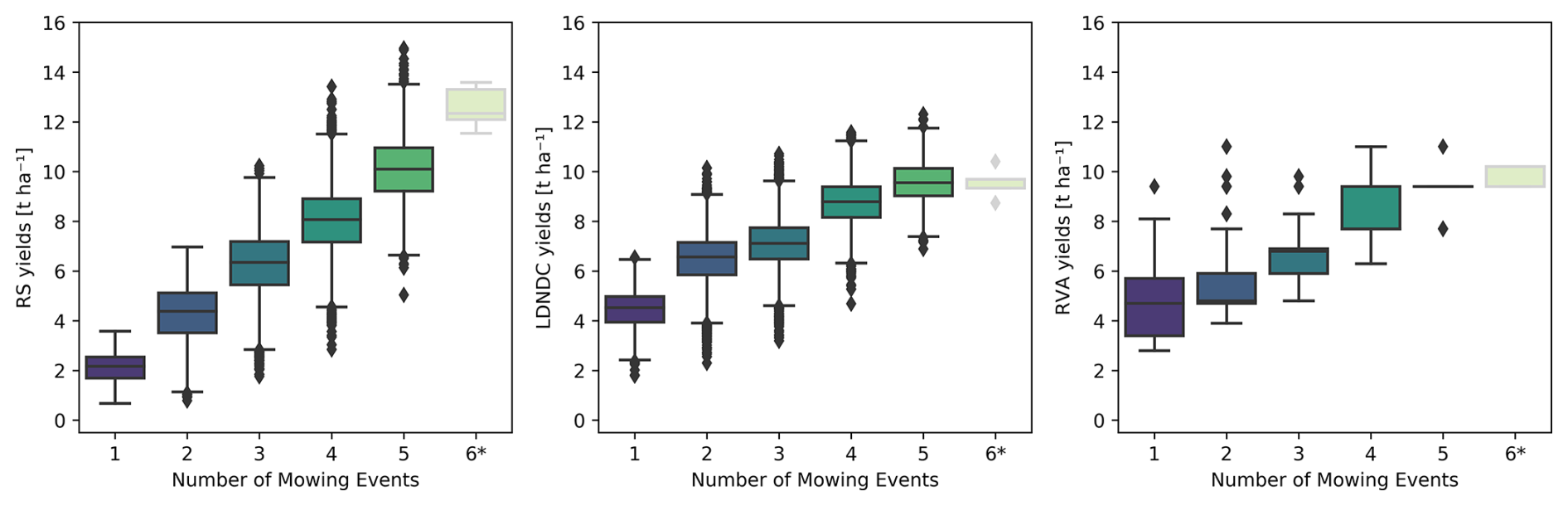
Figure 9 Estimated annual grassland yields per mowing frequency, based on the three models: RS, LDNDC and RVA. An asterisk (*) on the x axis denotes that only six parcels were mown six times per year which might not be representative.

4.3.2 Precipitation, temperature and elevation

The annual grassland yields increase with increasing mean annual temperature (MAT), mainly for RS and LDNDC and less for RVA (Fig. 10); however, the increase in yields is associated with a higher variability in yields for higher temperature classes. RVA yields stagnate at a MAT above 12.25 °C. The Pearson r value is significant for all relationships between the annual yield and MAT but generally show a low positive correlation (RS: r=0.2; LDNDC: r=0.26; RVA: r=0.1). The yields estimated by all three methods stay relatively constant for all precipitation levels present in the study region. Pearson's r values are −0.2 (RS), −0.18 (LDNDC) and −0.05 (RVA). Yield and elevation show a negative relationship, as annual yields decrease with elevation for all methods. Pearson's r values for the relationships between the estimated yields and elevation are −0.19 (RS), −0.23 (LDNDC) and −0.08 (RVA). However, for the RVA yield, estimates stay on average constant for an elevation of 500–900 m a.s.l. and only decline afterwards. Overall, the relationships between estimated yields and site conditions, such as temperature, precipitation and elevation, are relatively low and similar for the three methods (Fig. 10). These patterns stayed the same when the relationships were tested for individual mowing frequencies (see Fig. A3).

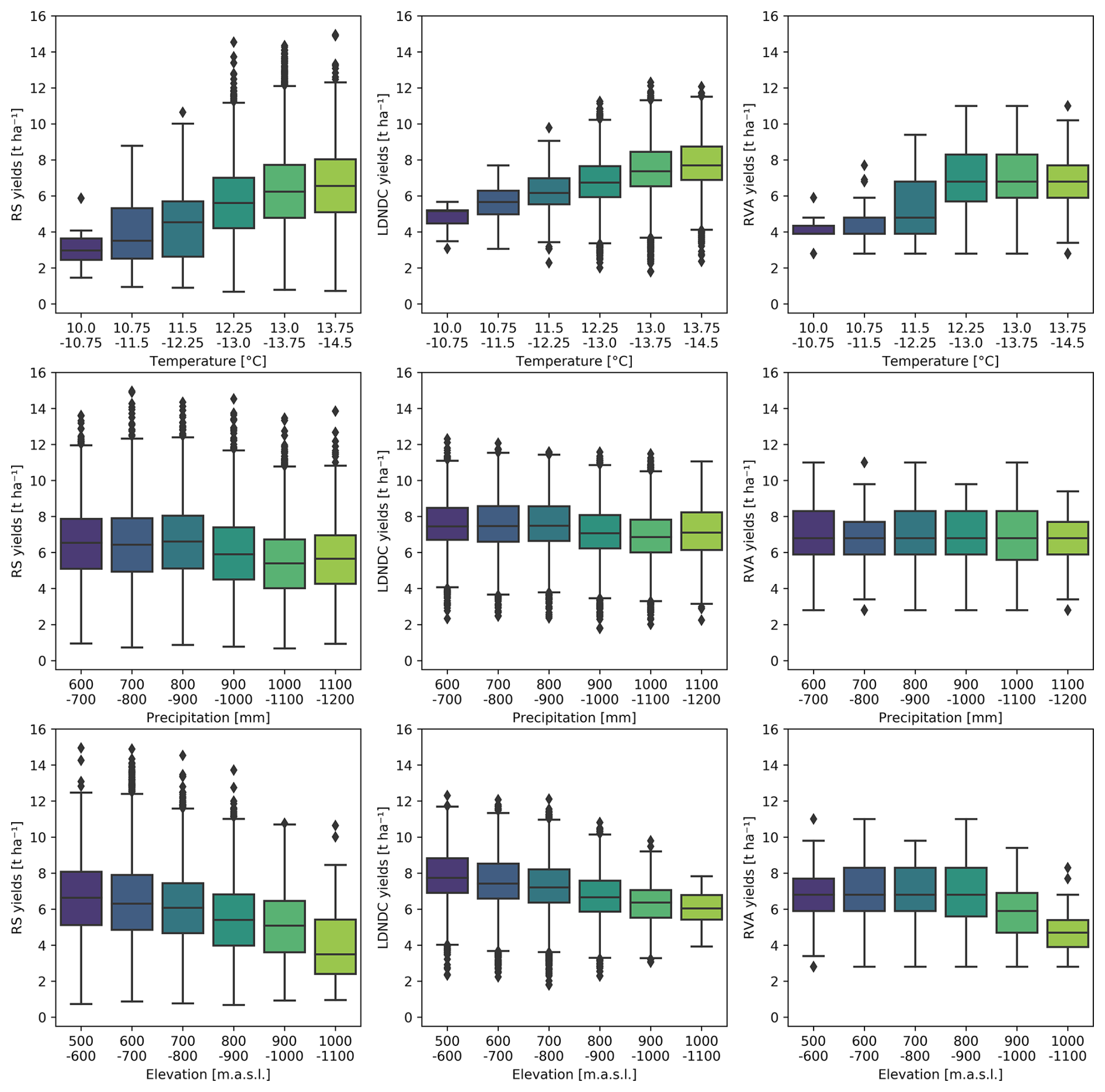
Figure 10 Aggregation statistics of estimated annual yields based on the three models per temperature, precipitation and elevation class.

5 Discussion

5.1 Performance of biomass modeling results

Despite the numerous studies on empirical grassland biomass modeling based on satellite and field data, only a few studies have been carried out in areas characterized by heterogeneous and small grassland parcels that are mowed multiple times on different dates during the year. Of these previous studies, the potential of various vegetation indices derived from medium-resolution sensors (MODIS and MERIS) to estimate grassland biomass for single sites in Ireland and the Netherlands were investigated (Ali et al., 2017b; Ullah et al., 2012). Based on Landsat and Sentinel-2 data, grassland biomass and height were estimated for study regions in Germany, France, Spain and Austria using various regressors, such as multiple linear regression, random forest or deep learning models, resulting in accuracies (R² values) of 0.45–0.79 (Barrachina et al., 2015; Dusseux et al., 2022; Eder et al., 2023; Muro et al., 2022; Schwieder et al., 2020). The performance of empirical models seems to depend more on the number of the training data and the variety of grassland types and use intensities included than on the tested regressors and model parameters. Regarding the tested indices and bands, wetness indices (Barrachina et al., 2015) and red-edge, near-infrared and shortwave infrared bands (Dusseux et al., 2022) were found to be valuable for grassland biomass modeling. With an R² of 0.68 for the test dataset, we reach comparable results with the RS approach. In our case, the R² of the cross-validation was relatively high (0.97); this might indicate overfitting, which should be avoided. As far as we know, information on the time since the last mowing event has not been included in previous existing studies. This parameter, however, was among the most important input features for the extreme gradient boosting model applied. Moreover, including information on mowing dates seems to be advantageous for grassland biomass estimation in study regions characterized by intensive grassland management.

The performance of LDNDC with respect to reproducing grassland yields of individual mowing events was found to be comparable to or better than other process-based models. For the annual yields, where regional input data were employed, the performance measures were even better than for single cuts. For further details, see Boos et al. (2024). We assume that the results for LDNDC can be transferred to other process-based models (e.g., Daycent and APSIM).

The comparison of the temporal patterns on estimated aboveground biomass shows that both results (RS and LDNDC) follow the mowing dynamics closely. This behavior is expected, as the mowing dates are directly included in both modeling approaches. However, the RS biomass estimates fluctuate more than those stemming from LDNDC and clearly depend on the availability of cloud-free satellite observations. LDNDC biomass values show a very high peak in the first growth cycle that is often double the value of the RS-based estimates. It is known from previous works that LandscapeDNDC overestimates yields from the first cut of the year and underestimates those of later cuts (Boos et al., 2024). However, it is also possible that the RS method underestimates the first-cut yield, as the AGB estimation might be prone to a saturation effect. In addition, AGB values at the higher end of the training data distribution are less likely to be predicted and strongly depend on a well-balanced training dataset.

Another important aspect that needs to be estimated is the AGB. Here, the goal was to estimate the biomass per cut, which corresponds to the yield. Farmers are generally advised to cut at 7 cm, although this can vary in practice. In the RS approach, the total AGB was used because the sensor only provides data from a certain height upwards. The LDNDC was calibrated using AGB samples taken from 7 cm. The cutting height for the reference values in the RVA approach likely varies considerably and cannot be reconstructed. Therefore, potential uncertainties due to AGB information from different cutting heights must be assumed.

5.2 Spatial patterns of annual grassland yield and influencing factors

The spatial yield patterns from all three methods match in some regions and differ in others. The spatial patterns mostly resemble the mowing frequency, which is a major influencing factor determining grassland yields (Bernhardt-Römermann et al., 2011). In many cases, areas with high yield match with areas showing a higher number of mowing events. For example, in the east or the north of the study area, for many grasslands, high annual yield estimates, in particular from the LDNDC and RS models, fit well to a large number of mowing events. This relationship is also underlined by the significant Pearson correlation coefficients of 0.66–0.81 between the annual yield and number of mowing events for the three models. Other regions, for example, east of Lake Starnberg and in the center of the study area, show high yield estimates but rather low to intermediate mowing frequencies (see Figs. 1 and 6). This discrepancy must be explained by other factors that influence grassland yields which were not looked into in detail here, such as soil conditions or an optimal interplay of influencing factors. Intensified mowing, usually accompanied by more fertilization, enhances biomass production and changes the species composition towards more productive, less diverse (lower number of species) vegetation in systems not strongly limited by other factors (Isbell et al., 2013; Mayel et al., 2021; Savage et al., 2021). The influence of site conditions, in particular climatic conditions, on the spatial annual yield patterns is twofold: firstly, the conditions in the year of interest influence vegetation growth in that particular year; secondly, climatic site conditions determine the species composition and management options of grasslands in the long term as well as soil properties like soil organic carbon. There are overall smaller yields visible in the south and southwest of the study region, matching the temperature patterns. Apart from that, the resemblance between annual yield maps and temperature, precipitation and elevation is relatively low (see Figs. 1 and 6). The Pearson correlation coefficients were significant but low for all combinations (−0.23 to 0.26). For correlation tests with as many data, as in our case, correlations tend to be significant (Rouder et al., 2009). It can be assumed that climatic effects have a more significant influence on grassland yields on a larger spatial scale, e.g., continental scale (Emadodin et al., 2021; Goliski et al., 2018; Zhang et al., 2018). Either the climatic gradients are not large enough in our study area to explain grassland yields or climatic conditions play only a minor role, as yields are mostly determined by management. A previously anticipated difference in the relationship between site conditions and yields for the three models (as LDNDC includes these data directly and RS captures the effects indirectly) was not found. Furthermore, in this study, only 1 year was examined that showed relatively normal climatic conditions. The differences between the models are most probably higher in extreme years, e.g., 2018, as extreme climatic effects can be depicted by LDNDC and RS but not by RVA (see Boos et al., 2024).

5.3 Differences between the modeling results

When comparing the annual yield values, the RS method leads to overall lower estimates compared to LDNDC and RVA, which can be explained in several ways. On the one hand, the RS method is prone to underestimation of annual yields, as the empirical model of aboveground biomass tends to provide underestimates. This is related to the available training data, which stem from field measurements throughout the year, with only a few samples from shortly before a mowing event. In this regard, the distribution of training samples might not be optimal and high-biomass data may be missing, resulting in an underestimation of the empirical model. In addition, the biomass estimation and the mowing detection are both dependent on the availability of cloud-free satellite observations. Biomass estimates from periods shortly before mowing events might be missed and, consequently, the yield related to the mowing event is potentially lower than in reality. Further, mowing events are potentially missed entirely due to cloud coverage (Reinermann et al., 2023) which additionally leads to these yields missing in the annual estimate. As the mowing information is included in all three approaches, missed mowing events due to clouds also affects the LDNDC and RVA yields.

On the other hand, while the RS method is more likely underestimating yields, LDNDC and RVA are more prone to overestimation. This is related to the fact that some factors which negatively influence vegetation growth and, therefore, yields are not included in the LDNDC and RVA models. For LDNDC, these are neglected local factors, like north-facing slopes and lateral runoff as well as the calibration on lysimeter data taken under favorable conditions (Haas et al., 2013). The input into the RVA model is very limited in the sense that local factors influencing the current growing conditions as well as yearly climate data are not included. Therefore, both models tend to represent optimal growing conditions and, hence, overestimate yields. Even though the RS model does not specifically address these factors, they are captured by the spatially varying reflectance signal.

When examining the lower yields resulting from the RS model compared to the other model estimates, it becomes clear that this effect is most prominent for grasslands mown one or two times per year (see Fig. 9). This could be related to a grazing effect. Such extensively used grasslands are very often also grazed (Schoof et al., 2020a, c). In the LandscapeDNDC simulations, the amount of grazed material remains on the field and leads to an overestimation of the yield from the next cut, either directly within the same year or via plant storage over the winter in the first cut of the following year. The RS method does not specifically account for grazing, and as the estimated biomass before mowing events is used, there is no such accumulation effect. Assuming that the difference between the RS and LDNDC yields of extensively used grasslands stems mostly from the grazing effect, it might be used to calculate grazed yields (e.g., Chang et al., 2015). The RVA considers grazing on mowed pastures. However, it follows a rather simple approach that estimates the grazing intensities using a farm's stocking rate. The stocking density, i.e., the number of LSU per hectare of field area, would be a more meaningful measure, but the IACS data do not include any information on the type of animal husbandry or grazing intensities. Therefore, yields of mowed pastures might be over- or underestimated in the RVA due to lack of detail in the information on grazing intensity.

It is also important to mention that all three approaches depend on mowing information as input data. RS and LDNDC use the mowing dates of grassland parcels in their algorithms, whereas RVA uses the mowing frequency. As the same mowing data were used for all three approaches, the results are comparable to each other. The importance of the mowing data for model performance is difficult to assess, as the methods do not work without them; however, one could investigate the impact of using various sources for mowing dates. In addition, there is also an uncertainty in the mowing data, as they were derived from the Sentinel-2 time series, which is prone to gaps due to cloudy weather conditions. The R² for the mowing detection in the study area is 0.65.

Other studies investigating grassland yield in Europe have mostly focused on the continental scale and have not been conducted at the parcel level. However, the estimated yields are in similar value ranges to our results (e.g., Chang et al., 2015; Smit et al., 2008).

5.4 Advantages and limitations of the approaches and implications drawn from them

All three approaches investigated in this study hold individual advantages and limitations to estimate annual grassland yields in southern Germany (see Table 1). The RS approach depends on well-distributed training data and cloud-free satellite observations. The value distribution of the training data determines the range of potential predictions of the empirical model and is, therefore, crucial. This also plays an important role with respect to the transferability (in space and time) of the approach. Without additional training data, the approach can hardly be applied in regions with different conditions. The necessity for satellite data can be particularly problematic for regions or time periods with relatively high cloud coverage. For instance, in Germany, the year 2021 was characterized by an overall relatively low number of cloud-free satellite observations, making the provision of satellite-data-based products, such as mowing detection or biomass estimation, more challenging (Reinermann et al., 2023). Despite these limitations, estimating grassland yields based on RS has several advantages. For example, even small-scale spatial effects are depicted, enabling the detection of parcels with reduced yields. Current spatiotemporal variation is mirrored, such as yield reduction through drought periods. In addition, despite the need for training data, no large input dataset or parameterization is needed for the RS approach, which might enhance the transferability.

Table 1 Overview of methodological properties, both advantages and drawbacks, comparing the three yield estimation approaches. The strongest relative fit between a method and property is indicated by $+++$, the weakest fit is indicated by +, and an asterisk (*) indicates “unknown”.

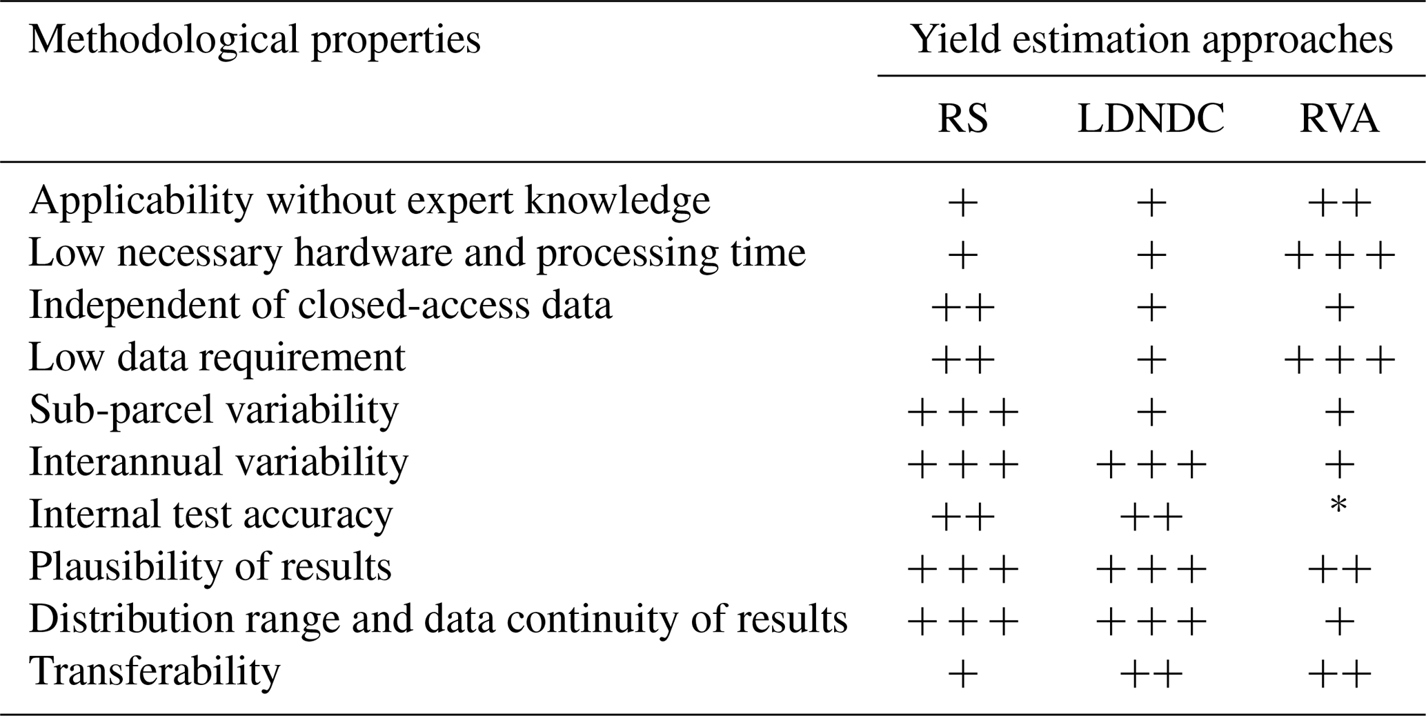
Major advantages of LandscapeDNDC – as a bio-geochemical model – are as follows: firstly, spatial and temporal variations are accounted for; secondly, the direct relation to input data, like climate, soil and air chemistry, is possible; thirdly, carbon, nitrogen and water budgets are modeled as well; and, lastly, scenarios (climate or management) can be studied. This also means that high-resolution input data (climate, soil, management and air chemistry) need to be available for the modeled domains. Generally, the model performs best if individual, detailed simulations are performed that are than aggregated to a larger spatiotemporal scale (e.g., field scale to hexagons). However, the slope and orientation as well as the species composition are not accounted for. To transfer the model, it is ideally recalibrated based on local measurements, although it has performed very well for crops (even on a global scale) without this step (Jägermeyr et al., 2021). For grasslands, so far, LDNDC has been used successfully in Switzerland, the UK and Germany (Houska et al., 2017; Molina-Herrera et al., 2016; Petersen et al., 2021).

The RVA is based on field measurements and mostly static input data, apart from the mowing frequency and stocking rate. Therefore, it is not able to depict spatial and temporal variations, such as drought episodes (Diepolder et al., 2016). It also needs input data such as the yield reference values, which are rarely provided on a larger scale. Further, cattle numbers, land use type (i.e., meadow or mowed pasture) and mowing frequency data are needed, which are – especially on scales larger than farm scale – difficult to obtain at times, as they are either not openly accessible or do not exist. An advantage of RVA is that the approach is relatively straightforward and does not need large amounts of computational power. Additionally, reference values are usually used by farmers to calculate their field's fertilizer requirements. The approach is, thus, more useful at the farm scale, where data can easily be obtained, and becomes more difficult to use at larger scales, due to restricted data availability.

All three approaches are, in a way, calibrated with regional data; therefore, their applicability is limited to regions with relatively similar grassland ecosystems. The RS approach relies on biomass samples, LDNDC relies on regional model calibration (input data) and RVA relies on the grassland index. As the management is highly relevant for the productivity and yield of grasslands in intensively used areas, such as in our study area, not only the geographic conditions and species composition but also the management strategies and use intensities of grassland ecosystems need to be comparable in order to transfer the calibrated models. Including additional ground-truth data from the target region for calibration would largely improve the transferability. However, the models also rely on data such as IACS or mowing data, which need to be available in potential target regions.

6 Conclusions and outlook

Within this study, the annual grassland yield was estimated for a study region in southern Germany in 2019 based on three different approaches: (i) an empirical remote-sensing model, (ii) a bio-geochemical model (LandscapeDNDC) and (iii) a rule-based reference value approach. It was shown that grassland yields can be estimated based on three completely different approaches, as plausible and comparable results were reached for the study area. The three models contain varying input datasets; however, all of them use mowing information as a driver. The mowing frequency was found to be the most important influencing factor for grassland yields in the study region for all three approaches.

Yield patterns and comparisons between the approaches showed that all three methods can be legitimately used for yield estimation (value ranges of approximately 4–9 t ha⁻¹) in pre-Alpine grassland ecosystems, considering individual limitations. All approaches need mowing information at the parcel level as input data. When a training dataset including well-balanced AGB samples and cloud-free satellite observations is available, it is advisable to use the RS approach. Depending on the training data distribution, the RS approach is capable of estimating grassland yields at the regional level and of capturing small-scale patterns at the field level (and beyond). LandscapeDNDC is also recommended for use at a regional or even continental level. Detailed data on climate, soil and management are needed and strongly determine the performance. For the field scale, the RVA can also be used, as the required data can be more easily obtained at the field level compared with at the regional level. To investigate single-cut yields only, RS and LDNDC can be used, as RVA solely provides an annual yield estimate.

The expected biases include a likely overestimation of the first-cut yield by LDNDC and an underestimation of the first-cut yield and, to a lesser degree, annual yields in general by the RS approach. To investigate yield patterns over time, only RS and LDNDC are useful, as the RVA does not include actual conditions. Improved grassland yield estimations could be obtained with more AGB sample data, in particular when analyzing years with climatic extremes, as the AGB data might not be representative. In addition, validation data on annual grassland yields would be needed to evaluate the approaches in more detail.

The study presents synergies of grassland yield estimation approaches; this is particularly important because spatial information on grassland yield is limited. Based on robust grassland yield estimations, multiyear analyses can be conducted and the effects of factors such as climate change can be investigated. In addition, a comprehensive understanding of grassland ecosystems is facilitated, thereby supporting authorities and science.

Appendix A:  

Table A1 Bavarian reference values for farmers' grassland yield from field measurements for meadows and mowed pastures of different use types and yield levels.

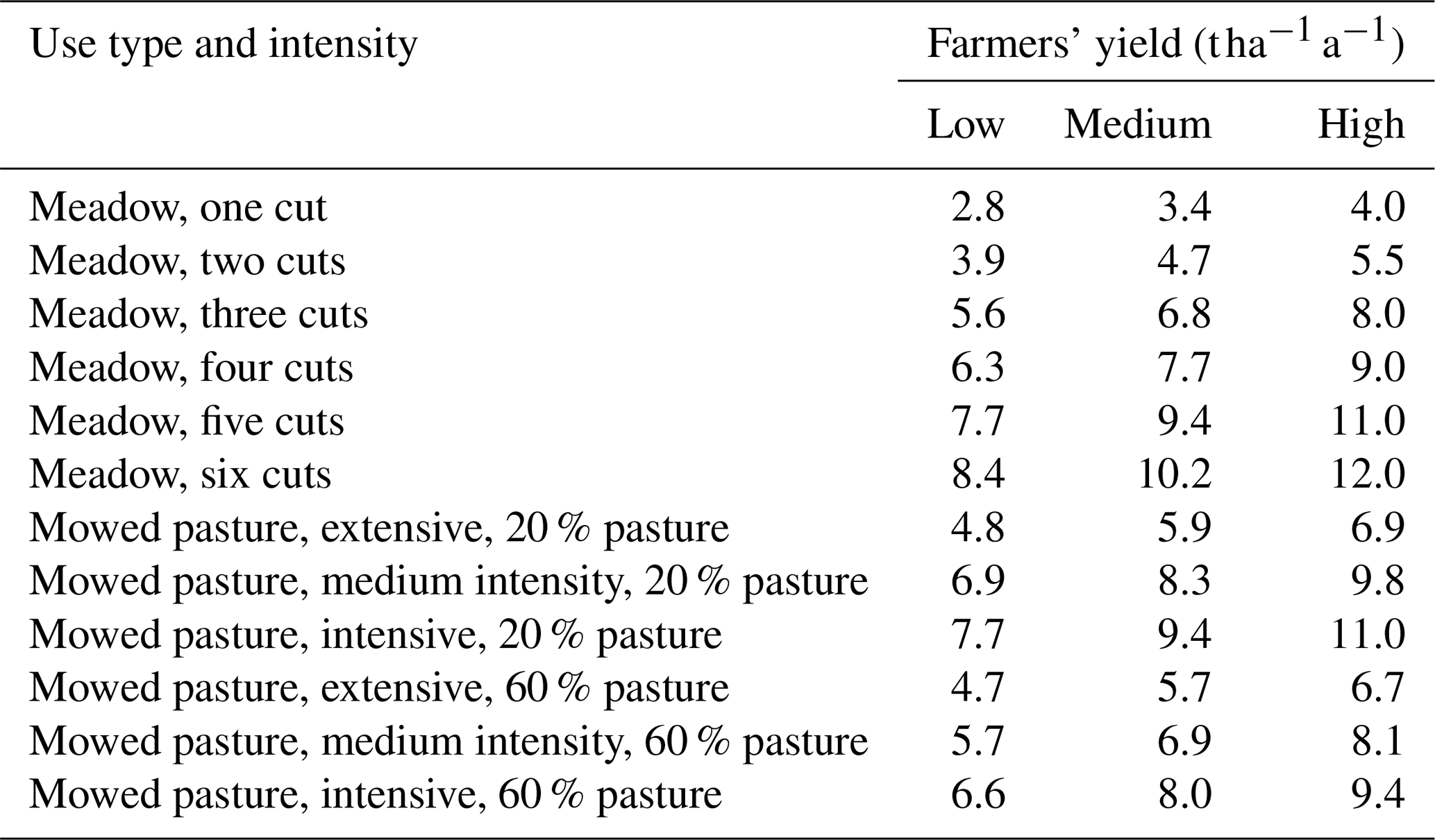
Table A2 Grassland yield level/grazing intensity according to grassland index and slope stocking rate which is used as input for Table A1.

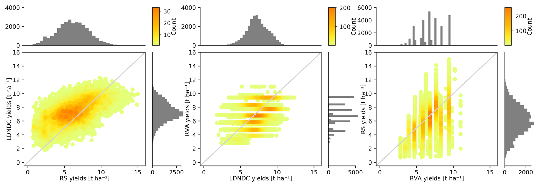
Figure A1 Pairwise relationships of parcel-level annual yield estimates for meadows and mowed pastures in the study area in 2019 based on remote sensing, LandscapeDNDC simulations and the reference values approach with histograms of the three modeling approaches. Note that the color ranges differ for the subplots.

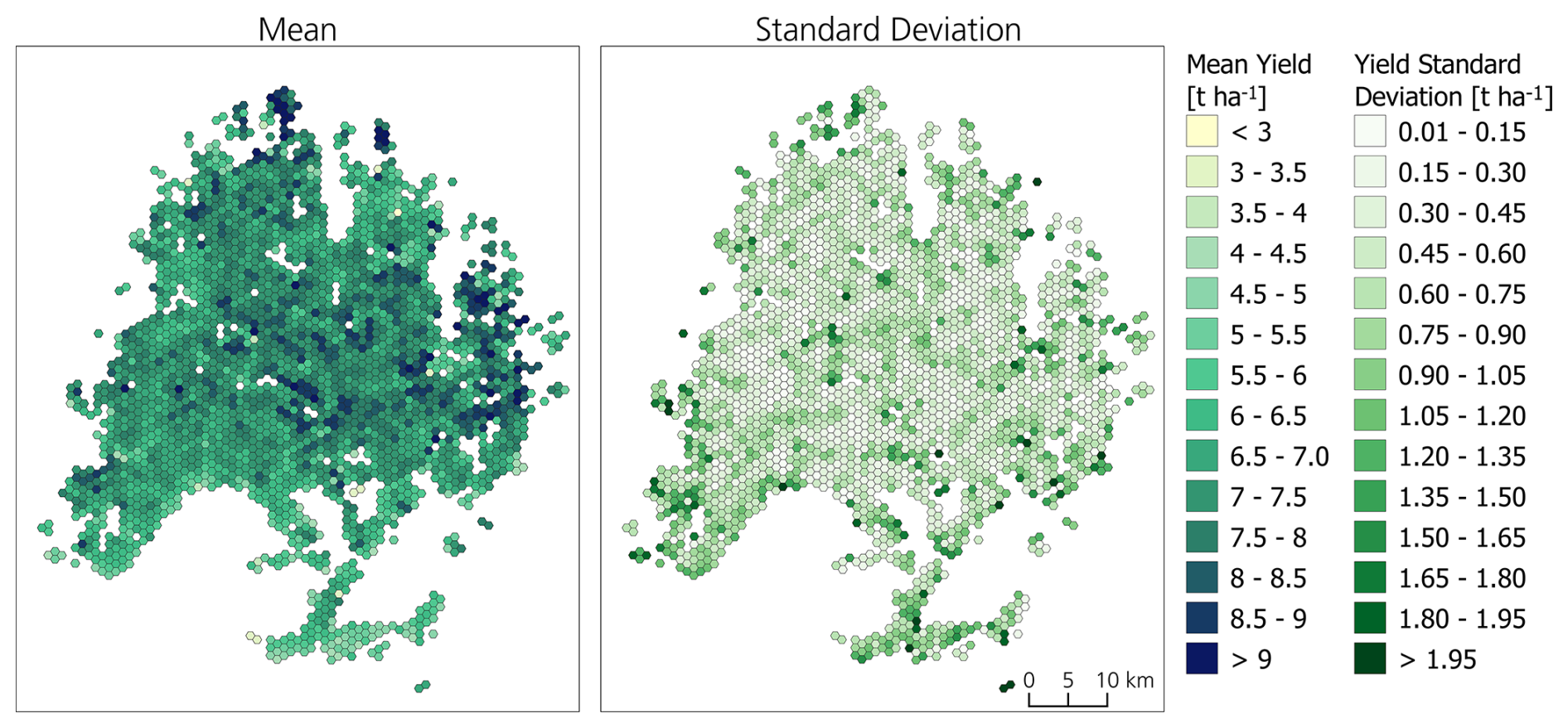
Figure A2 Mean and standard deviation of spatially aggregated (hexagon diagonal length of 1 km) annual yield estimates for meadows and mowed pastures in the study area in 2019 for all three approaches. Hexagons for which the grassland area is smaller than 1 ha are not shown.

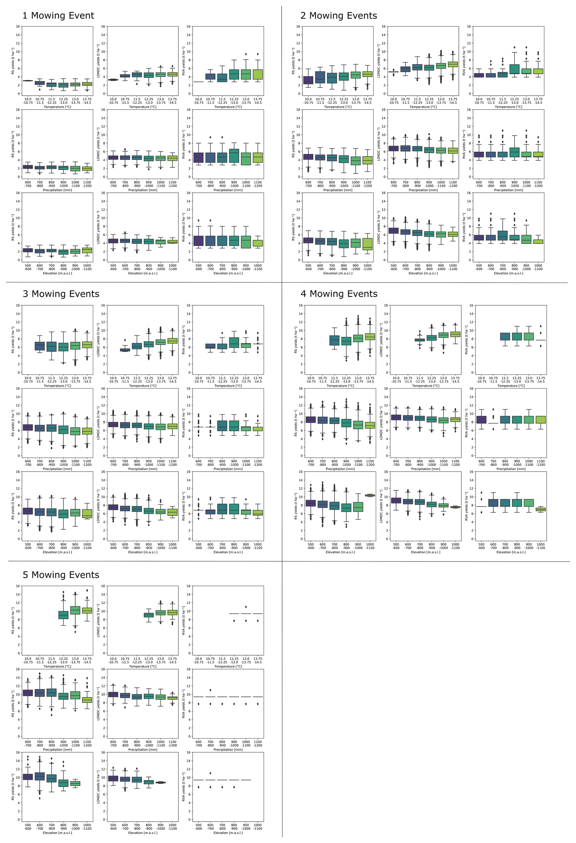
Figure A3 Aggregation statistics of estimated annual yields based on the three models per temperature, precipitation and elevation class for grasslands mown one to five times per year.