the Creative Commons Attribution 4.0 License.
the Creative Commons Attribution 4.0 License.
 | 18 Feb 2026
Evaluating the consistency of forest disturbance datasets in continental USA
Franziska Müller
Ana Bastos
Forests play a crucial role in the Earth System, providing essential ecosystem services and sustaining biological diversity. However, forest ecosystems are increasingly impacted by disturbances, which are often integral to their dynamics but have been exacerbated by climate change. Despite the growing concern about these trends, the lack of consistent and temporally continuous data on forest disturbances at large spatial scales hinders our ability to accurately characterize changes in disturbance regimes and respond to these changes.
In this study, we evaluate the consistency in spatial distribution and extent, disturbance timing and causal agent (when available), of five forest disturbance datasets available for the conterminous United States, to identify advantages as well potential shortcomings and inaccuracies of different mapping approaches. Consistency refers to the extent to which different forest disturbance datasets report similar timings and causal agents for overlapping disturbance events, reflecting their level of agreement. Specifically, we compare data from the Forest Inventory and Assessment (FIA), the Insect Disease Survey (IDS), both regularly conducted by the U.S. Department of Agriculture (USDA), the literature survey by the International Tree Mortality Network (ITMN) and two satellite-based datasets, the Global Forest Change (GFC) and North American Forest Dynamics Forest Loss Attribution (NAFD). All datasets report disturbance timing with a temporal granularity of one year, FIA and ITMN are point-based, and IDS, GFC and NAFD are spatially explicit. FIA, IDS, ITMN and NAFD report on disturbance agent, with different classification groupings.
We find a moderate spatial agreement between the spatially explicit datasets and the point-based ones, with IDS, GFC and NAFD overlapping with 24 %, 58 % and 42 % of FIA disturbed patches, and on average 35 % of the ITMN reported mortality events. The datasets show similar trends in total disturbed extent over conterminous USA (CONUS) for the common period of 2001–2010, but with more pronounced differences at smaller scales, and when accounting for disturbance agents. The datasets agree well in disturbance timing: the mean difference is less than one year, while the variability in differences ranges from about 1 to 4 years. For FIA, we find better agreement with other datasets when the disturbance timing coincides with the inventory year, compared to disturbances reported as occurring in years between inventories. The satellite-based datasets tend to show an earlier detection of disturbance events, compared to the other datasets, possibly due to the inconsistent revisiting times of the inventory datasets (FIA and IDS).
Our results show that although the datasets exhibit reasonably good agreement in disturbance timing, their spatial correspondence is considerably lower. Furthermore, the datasets show low agreement in terms of disturbance agent, which results from differences in grouping but also potentially on the methodology used to report causes. Our findings thus underscore the importance of careful data quality assessment and consideration of their inherent uncertainty when using single forest disturbance datasets for further applications. Specifically, for smaller scales and for disturbance agent attribution, we recommend careful comparison of more than a single dataset. Our study further highlights the need for improved data integration to advance the understanding of changes in forest disturbance regimes and their drivers.
- Article
(9396 KB) - Full-text XML
-
Supplement
(341 KB) - BibTeX
- EndNote


Forests play an important role in the Earth System as they provide ecosystem functioning and services, serve as a carbon sink and support biodiversity (Bonan, 2008; Lindner et al., 2010). These services – including provision of food and water, climate regulation, and cultural services – are essential for society and help preserve the biological diversity of forests (Thom and Seidl, 2016).
Forest disturbances such as forest fires or insect infestations, are integral parts of forest ecosystems and have significant impacts on forest functioning, structure, composition and dynamics (Turner, 2010). Ecosystem disturbances have been defined in various ways in the literature, with one of the most widely cited definitions provided by White and Pickett (1985), who describe disturbance as “any relatively discrete event in time that disrupts ecosystem, community, or population structure and changes resources, substrate availability, or the physical environment”. In the inventory datasets used here, disturbances encompass not only tree death, but also early indicators such as discoloration and crown dieback. For comparability across datasets, here, we consider disturbance as any event that causes tree mortality. Thom and Seidl (2016) found that the impacts of disturbances on ecosystem services are generally negative across all categories of services. Given their impact on forest productivity, growth, mortality and composition, disturbances can further feed-back to climate through changes in forest carbon balance (Bowman et al., 2009; Hicke et al., 2012). At the same time, Thom and Seidl (2016) also reported that disturbances can have beneficial effects on biodiversity, showing neutral to positive impacts on species diversity, species richness, and habitat quality. These findings highlight the complex nature of disturbances, which can simultaneously compromise ecosystem services and support biodiversity.
The 2000s have seen an increase in hotter and prolonged droughts due to climate change (Allen et al., 2015; Masson-Delmotte et al., 2021), along with reported increases in climate-driven forest disturbances such as bark beetle outbreaks, storms and fires, impacting forest ecosystems across all forested continents (Seidl et al., 2017; Patacca et al., 2023; Hartmann et al., 2022). Changes in the frequency, size, and severity of these disturbances driven by climate change can alter forest functioning, affect the provision of forest services (Turner, 2010; Meigs et al., 2017; Seidl et al., 2017; Kautz et al., 2017) and threaten forest stability (McDowell et al., 2020; Seidl and Turner, 2022). Beyond the effects of climate change, anthropogenic factors also play a key role in shaping disturbance patterns. Changes in land-use practices, forest management, and afforestation efforts modify forest extent, composition, and age structure, ultimately influencing how forests respond to disturbance (Seidl et al., 2011).
Disturbance impacts can intensify when extreme climatic events coincide with high forest susceptibility or other preconditioning factors (Seidl et al., 2011; Bastos et al., 2021). Understanding and quantifying the combined effects of compound drivers is essential for predicting and mitigating future changes in disturbance regimes and their impacts on forest ecosystems (Bastos et al., 2023). However, we currently lack globally consistent and temporally continuous data over periods sufficiently long to characterize changes in disturbance regimes, especially when it comes to biotic disturbances and wind (Kautz et al., 2017). Multiple datasets record and document multiple natural and human disturbances, often in the same state/continent, but with different methods. Current forest disturbance information is based on sparse and discontinuous data (Kautz et al., 2017; FAO, 2010, 2015, 2020; Hammond et al., 2022), although more comprehensive datasets have been compiled for certain regions (Hicke et al., 2012; Patacca et al., 2023; Forzieri et al., 2023; Senf and Seidl, 2021b, a).
Forest disturbance datasets currently available can be grouped into two groups: ground survey and inventory data (Forzieri et al., 2023; Patacca et al., 2021; Forest Service U.S. Department of Agriculture, 2024, 2023) and remote-sensing based datasets (Hansen et al., 2013; Senf et al., 2020). Existing forest disturbance data differ in the attribution of disturbances, the details in information/records and the acquisition methods. Inventories provide detailed information about the disturbance location, extent, timing and agents, collected through aerial detection and ground surveys, but are sparse in space and time, and suffer from several uncertainties, e.g., due to differences in reporting methods, sampling strategies, human errors, etc. (Hammond et al., 2022; Coleman et al., 2018; Tinkham et al., 2018). Remote sensing, in turn, offers the possibility to monitor large regions (up to the globe) in a spatially and temporally consistent manner. However, the accuracy of satellite-based disturbance mapping depends on the spatiotemporal resolution of the sensor, on the intensity of the disturbances, as well as the disturbance size and underlying forest structure (McDowell et al., 2015). Therefore, large-scale datasets typically consider stand-replacing disturbances (Senf et al., 2020; Hansen et al., 2013) and attribution to specific agents is limited (Senf and Seidl, 2021b). Attribution of satellite-based disturbances to specific agents requires, however, high-quality ground data for calibration and validation, underscoring the importance of inventory data in supporting the development of disturbance classification and prediction models (Forzieri et al., 2023; Andresini et al., 2024; Bárta et al., 2021; Hawryło et al., 2018; Gibson et al., 2020).
Characterizing the uncertainty of these different datasets is crucial given their wide range of applications, e.g., carbon cycle, forest productivity and growth, forest health, and climate (Harris et al., 2016; Tinkham et al., 2018; Knott et al., 2023; Cohen et al., 2016; Schleeweis et al., 2020; Schroeder et al., 2014; Thompson, 2009). For example, Hicke et al. (2020) used data from the Insect and Disease Survey (IDS) by the Forest Service of the U.S. Department of Agriculture (USDA) to characterize bark beetle outbreaks in the western United States. They highlighted that uncertainties and inconsistencies in the records arise due to variations in surveyor methods, survey locations, and flying conditions. They partially addressed these issues by incorporating specific assumptions into their analytical framework, but they could not account for example for the year-to-year variability. Coleman et al. (2018) investigated the accuracy of the IDS data by comparing aerial detection survey data with ground survey records and high-resolution satellite imagery (WorldView-3). They used error matrices to assess accuracy across different categories. Their findings indicated variable accuracy among damage types and damage agent genera, with bark beetles, the most abundant genera, exhibiting some of the largest errors. Overall, they found that 75 % of the damage was mapped correctly. However, the aerial detection survey polygons only overlapped with 44 (±0.06) % of ground observations.
Uncertainties in aerial detection, such as year-to-year variability (Hicke et al., 2020) and accuracy limitations (Coleman et al., 2018), highlight two needs. First, integrating ground-based observations with high-resolution satellite imagery might improve the consistency, accuracy, and detail of agent information of disturbance detection through data fusion. Second, a better quantification and understanding of the uncertainties within existing ground-based datasets remains essential, particularly as these datasets are used to train machine learning models that extrapolate disturbance patterns across broader regions (Senf et al., 2015; Forzieri et al., 2021, 2023; Patacca et al., 2023; Schleeweis et al., 2020).
In this study, we focus on the conterminous USA (CONUS), a region where multiple forest disturbance datasets are available. We aim to quantify the robustness of the information on disturbance extent, timing and respective agents, and to identify advantages, potential shortcomings and inaccuracies of different approaches, including widely used remote-sensing based datasets and more detailed ground-based inventories. Specifically, we compare the temporal and spatial consistency of five different forest disturbance datasets in the time period from 2001 to 2010. Most datasets include information on broad groups of disturbance agents such as wind, fire, insects, drought, although with different thematic foci. These datasets are grouped into two categories based on their spatial representation: spatially explicit datasets – including the Insect and Disease Survey (IDS) by USDA (Forest Service U.S. Department of Agriculture, 2024), the Global Forest Watch (GFC) tree cover loss product (Hansen et al., 2013), and the North American Forest Dynamics Forest Loss Attribution dataset (NAFD) (Schleeweis et al., 2020) – and point-based datasets, which comprise the Forest Inventory and Analysis (FIA) program by USDA (Forest Service U.S. Department of Agriculture, 2023) and tree mortality records from the International Tree Mortality Network (ITMN, Hammond et al., 2022).
This grouping reflects fundamental differences in dataset types. Spatially explicit datasets based on remote sensing, such as GFC and NAFD, provide pixel-level information, enabling detailed mapping of disturbance extent and location with broad geographic coverage and temporal consistency. However, optical remote sensing data have reduced capacity to capture small-scale or subtle disturbances, such as low-intensity selective logging that removes only a few trees. These minor canopy openings are spatially diffuse and short-lived, making them difficult to detect from spectral signatures in satellite imagery. Sub-canopy structural changes likewise remain largely invisible to optical sensors (Gao et al., 2020). Point-based datasets, including FIA and ITMN, consist of plot-level observations that capture ground-level details of disturbance agents and timing, though with coarser spatial coverage and uneven sampling. IDS combines elements of both approaches, offering detailed spatial inventories from ground surveys and aerial detection, with attribution of disturbance agents. The complementary strengths and limitations of these dataset groups motivate their combined use. Inventory data – both spatially explicit (IDS) and point-based (FIA, ITMN) – are critical for agent attribution and for validating remote sensing products. At the same time, differences in data collection protocols, revisit intervals, agent definitions, and property ownership can introduce uncertainties, which are explored in this study.
By comparing these five forest disturbance datasets, we aim to highlight the variability and underlying uncertainties associated with different observation systems. Our goal is to provide a systematic assessment of their consistency in disturbance extent, timing, and agent attribution. Through this comparison, we seek to identify dataset-specific limitations and offer guidance on their use, for instance, by incorporating uncertainty ranges for disturbance timing or by combining complementary datasets to improve spatial reliability. Although our analysis focuses on the conterminous United States, the approach is transferable to other regions and can inform the design of more robust, uncertainty-aware forest monitoring and classification frameworks (European Commission: Directorate-General for Environment et al., 2020).
2.1 Study area
This study focuses on the conterminous USA due to the availability of various forest disturbance datasets. Alaska is excluded because of limited data coverage. Figure 1 shows the study area in panel (A) (CONUS), with panels (B)–(E) providing a detailed view of a selected region (highlighted as a square in panel A) to illustrate the spatio-temporal characteristics of the different datasets.
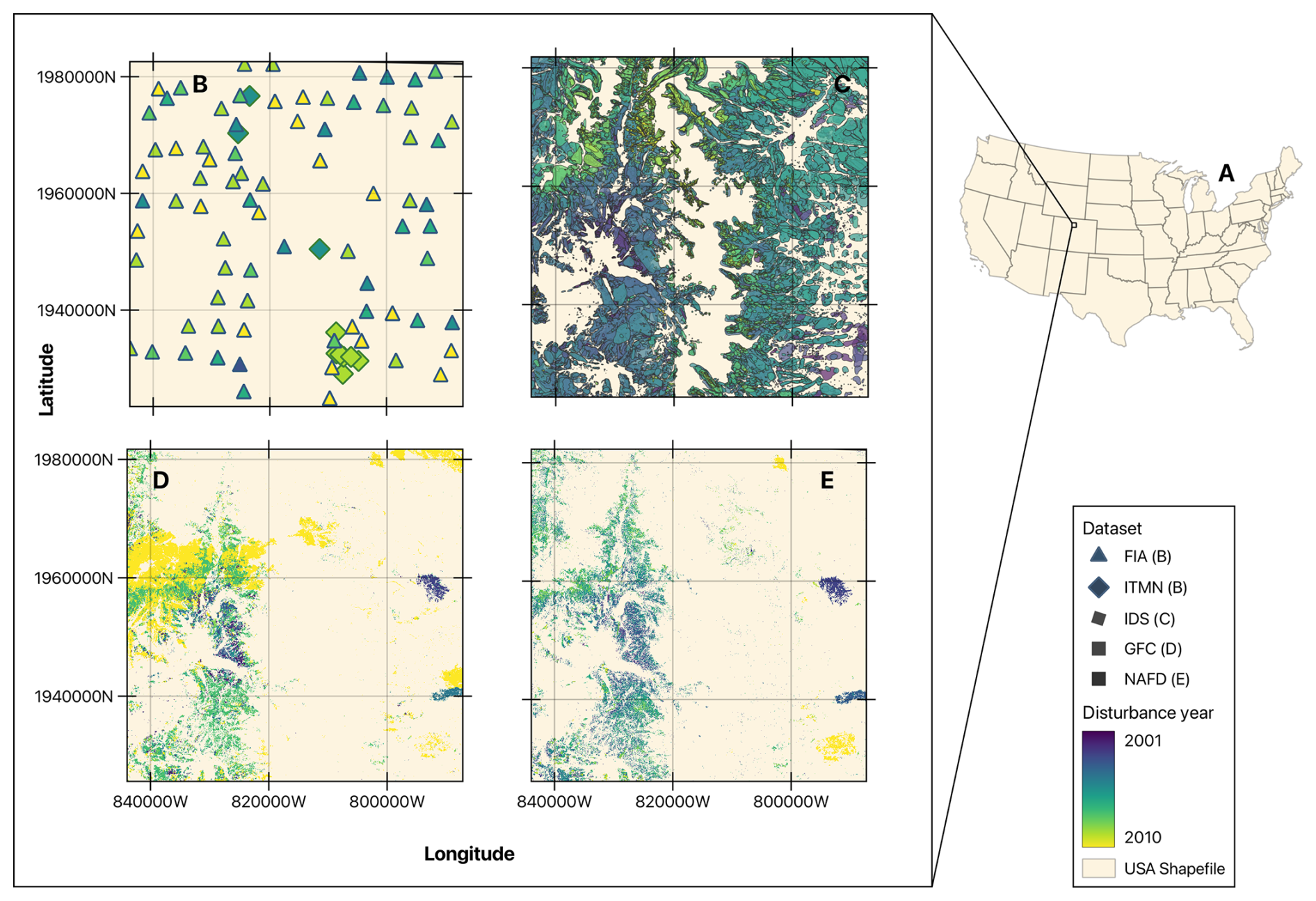
Figure 1Study area and illustration of the different datasets used in this study for a representative area. Panel (A) shows the study area of this study (CONUS), with an inset outlining a representative area where all five datasets report disturbances in the common period 2001–2010, shown in panels (B)–(E). All datasets use a consistent color scheme, with disturbance events in 2001 in purple to events in 2010 in yellow. Panel (B) illustrates the point-based datasets, with FIA represented by triangles and ITMN by diamonds. Panels (C), (D), and (E) display the spatially explicit datasets individually to facilitate comparison: IDS disturbance polygons in panel (C), GFC in panel (D), and NAFD in panel (D).
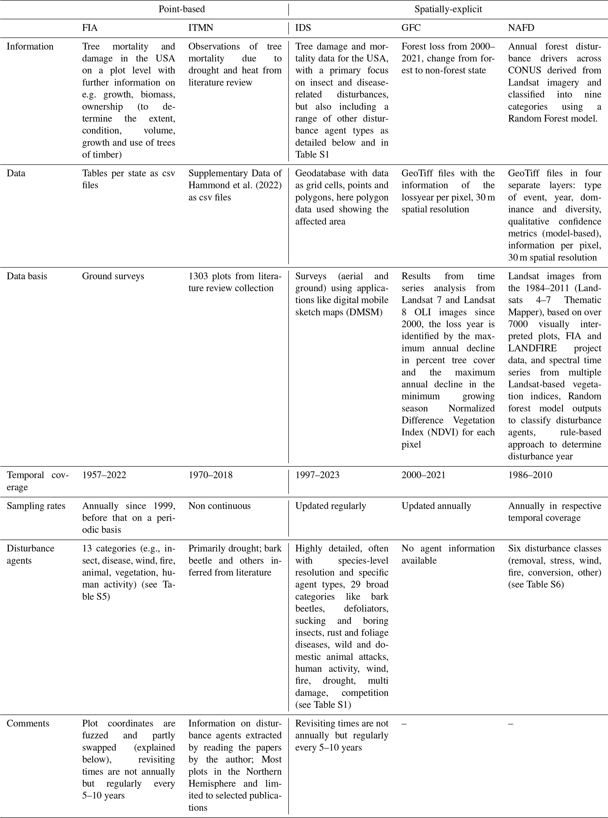
We provide an overview of the five datasets used in this study (see Table 1), including the information in each dataset, their data format and additional characteristics in the sections below.
Hammond et al. (2022)Table 1General overview of the five datasets used in this study, including the type of information provided, data format, collection methods and temporal availability.
2.2 Forest Inventory and Analysis
The Forest Inventory and Analysis (FIA) program of the USDA Forest Service Research and Development Branch, started in 1929 when data on the extent, condition, volume, growth and the use of trees in the Nation's forest land was collected on a periodic basis. In 1999 the program moved to an annualized inventory system. Since then, data is collected and compiled in a consistent tabular format, spanning all states and inventories. The current table structure is derived from the National Information Management System (NIMS) to process and store annual inventory data. The data is captured at various levels, including broad information such as location, tree species, invasive species and population, along with more detailed tables that provide specific information on conditions, plot and tree measurements, disturbances, agents, and ground cover (Burrill et al., 2021). The tables and columns of interest for this analysis are presented in Tables S2–S4 in the Supplement.
The FIA data provides information on plot ownership (public vs. private forests) as well as the year of tree mortality, measurement, and inventory, allowing to assess how these variables contribute to the discrepancies observed between datasets. For our analysis, we used the reported mortality year, which represents the estimated year a measured tree died or was cut. The inventory year is a reporting variable that denotes the year best representing when a group of plots was sampled at the program level, whereas the measurement year refers to the calendar year in which field measurements for an individual plot were completed during a site visit. Sampling intensity and measurement rates can vary across and within FIA regions, states, and measurement years due to operational and budgetary constraints (Burrill et al., 2021; Hou et al., 2021). Consequently, while plots may be repeatedly measured within less than a year, the revisiting frequency for FIA plots could range from 5 to 10 years (Schroeder et al., 2014).
Data are sampled in 1-acre plots, each typically containing four 7.3 m (24.0 ft) radius subplots, where trees with a diameter at breast height (DBH) over 12.7 cm (5.0 in) are measured. To protect landowner privacy, plot coordinates are intentionally imprecise. The FIA applies a “fuzzing and swapping” method: coordinates are shifted within a 0.8 to 1.6 km radius (fuzzing), and up to 20 % of private plots are swapped with another similar plot within the same county. This maintains county-level summaries and ownership class but introduces spatial uncertainty. To assess the impact of this uncertainty, we evaluate whether swapping affects results and compare FIA data with other datasets using buffer zones of 800 and 1600 m.
2.3 International Tree Mortality Network
The International Tree Mortality Network, in the following referred to as ITMN, was created to advance the development of methods for combining, harmonizing, and integrating various data repositories and data types to provide comprehensive information on global tree mortality rates (International tree mortality network, 2022). This effort involves both terrestrial and remote-sensing data sources. It therefore also relies on the contributions of other scientists to enrich the network with diverse data and expertise. The ITMN first compilation of heat and drought induced tree mortality is based on a literature review of 154 peer-reviewed studies since 1970 and data requests as described by Hammond et al. (2022). The dataset has been published in a geo-referenced database with records of tree mortality events (International tree mortality network, 2022) and includes 1303 plots of recorded tree mortality from 1970 to 2018 as point data. Each record includes the reported mortality year, along with location, reference publication, continent, number of sites and plots, and biome information. The study notes a potential bias in the dataset, as it is based solely on available peer-reviewed studies, which in the case of the USA predominantly report drought- and heat-induced tree mortality events.
2.4 Insect and Disease Detection Survey by USDA
The Insect and Disease Detection Survey the U.S. Department of Agriculture (USDA) is a database on forest damage and mortality due to different disturbance causing agents (Forest Service U.S. Department of Agriculture, 2024). While it primarily focuses on insect and disease-related impacts, it also includes other categories such as abiotic damage from fire, wind, drought, and geological causes, as well as disturbances linked to human activities, animals, and competition. In the following, we refer to this dataset simply as IDS (Insect and Disease Survey).
In the IDS dataset, the continental United States is divided into nine major regions, which are surveyed annually through both aerial detection and ground observations. Data collection relies on applications such as the Digital Mobile Sketch Mapping (DMSM) and the Southern Pine Beetle (SPB) Collector Map. In the DMSM, forest disturbances are documented by sketching the extent of tree injuries and mortality, storing the data as geo-referenced points or polygons. In addition to mapping the affected areas, surveyors record key attributes, including tree species, disturbance agents, damage types (e.g., defoliation, mortality, discoloration), and disturbance severity. The IDS dataset includes 29 broad categories of disturbance agents, as shown in more detail in Table S1. These categories encompass various insect types (e.g., bark beetles, defoliators, sucking and boring insects, fruit insects, gallmakers, and predatory insects), multiple disease classes (such as rusts, cankers, root diseases, and general diseases), and a range of other disturbance agents. These include abiotic and biotic damage, animal impacts (from both wild and domestic animals), fire, wind, drought, competition, human activities, multiple damage types, and unknown causes. During aerial surveys, geo-referenced base layers such as aerial photographs, topographic maps, and near-infrared imagery are used to track surveyor positions, improve disturbance detection, and avoid duplicate mapping of previously recorded damage. The database contains vector data in the form of both polygons and points representing recorded disturbances. We focus specifically on polygon data and use the survey year – the year in which the aerial survey was conducted – as the disturbance year for all records, since no explicit mortality year is provided in the dataset.
2.5 Global Forest Change
The Global Forest Change (GFC) provides annual maps of global forest change (net, gains and loss) at approximately 30m spatial resolution since 2001 (Hansen et al., 2013, 2024). Here, we focus on the loss year variable. Forest loss is defined as a stand-replacement disturbance or the complete removal of tree cover canopy at the Landsat pixel scale (Hansen et al., 2013). Based on time series from Landsat 7 and Landsat 8 OLI images, the year of tree loss is identified by the maximum annual decline in percent tree cover and the maximum annual decline in the minimum growing season Normalized Difference Vegetation Index (NDVI) for each pixel.
The data are provided in georeferenced raster files organized in 10×10° latitude/longitude tiles (Hansen et al., 2024). They calculate time-series spectral metrics and apply a decision tree model that links these metrics to observed canopy changes. Forest loss is disaggregated to annual time steps by identifying the maximum yearly decline in percent tree cover and in minimum growing season NDVI. The pixel values range from 0 to 21, indicating the year of forest loss, whereas 0 is no change (year 2000 as initial year), therefore the first year with changes can be 2001. The dataset does not specify the causes of forest loss, but it includes all disturbances that result in stand-replacing changes. For example the tropics are predominantly affected by the prevalence of deforestation dynamics due to shifting agriculture and commodity-driven deforestation (Hansen et al., 2013; Curtis et al., 2018; DeFries et al., 2010). In extratropical regions (temperate, boreal), tree cover loss is determined by forestry, fires, logging, diseases, and storms, at more moderate rates (Hansen et al., 2013; Curtis et al., 2018; Potapov et al., 2008; Sommerfeld et al., 2018).
2.6 North American Forest Dynamics Forest Loss Attribution
A second dataset based on Landsat satellite data used in this study is the North American Forest Dynamics Forest Loss Attribution (NAFD-ATT) based on Landsat imagery and spanning the conterminous United States from 1986 to 2010 (Schleeweis et al., 2020). This dataset is part of the North American Carbon Program (NACP), a multidisciplinary research initiative focused on carbon dynamics across North America. The NAFD-ATT dataset includes four data layers, of which the first two – disturbance type and year of disturbance – are most relevant to this analysis. NAFD-ATT estimates the drivers of forest canopy cover loss on an annual basis using a machine learning model and Landsat imagery at a 30 m spatial resolution. The disturbances are classified into nine categories, six of which represent actual causes of canopy loss. The NAFD disturbance agents include Removal, Fire, Other, Stress, Wind, and Conversion. Removal and Conversion both represent human-driven clearing, with Conversion specifically indicating a subsequent change in land cover or land use. Stress can be “any event resulting in slow gradual loss of forest canopy, including insect damage, drought and disease” (Schleeweis et al., 2020). The authors used training data from over 7000 plots across the United States, where forest change was visually labeled using annual Landsat image time series and TimeSync software. Additional training data came from FIA ground data, the LANDFIRE project – a database about fuel treatment, restoration, and suppression planning – and expert interpretation using the TimeSync software. They used change detection algorithms to capture different types of forest disturbance (e.g., abrupt clearings, gradual declines, fire). These algorithms were applied to Landsat time series stacks derived from various spectral indices, including the Normalized Difference Vegetation Index (NDVI), Band 5 surface reflectance, the Forestness Index (FI), and the Normalized Burn Ratio (NBR). These outputs, along with environmental and vegetation data, were used as predictor variables in a Random Forest model to classify disturbance agents, and a rule-based approach was applied to determine disturbance year and duration. The data are provided as individual GeoTIFF files covering the entire CONUS region (Schleeweis et al., 2020). In the following we refer to this dataset simply as NAFD.
2.7 Digital Elevation Model
We use the U.S. Geological Survey (USGS) 1 arcsec Digital Elevation Model (DEM) (U.S. Geological Survey, 2025) to evaluated whether the temporal agreement between dataset comparisons depend on topographic effects on the remote-sensing signal. The DEM provides a bare-earth representation of terrain at approximately 30 m resolution. We use the most current elevation files from the staged product series, with publication dates ranging from 2013 to 2023 depending on the file.
The following flowchart (Fig. 2) shows the steps per dataset from pre-processing to the final tables, which will be further explained below. All calculations are done in Python using the packages pandas, numpy, geopandas, scipy.stats. The code will be made publicly available upon acceptance.
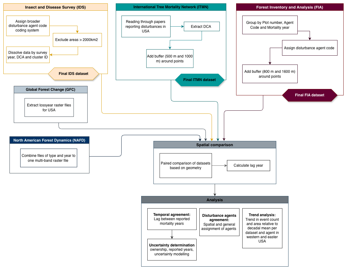
Figure 2Flowchart of dataset-specific preprocessing, harmonization, and analysis steps used to compare forest disturbance timing, location, and attribution.
3.1 Data pre-processing
In order to be compared, the datasets are pre-processed individually, depending on the type, complexity and detail of the information within each dataset. The GFC dataset did not require any pre-processing given that it is a georeferenced raster dataset with only one layer of information.
3.1.1 Disturbance agent classification
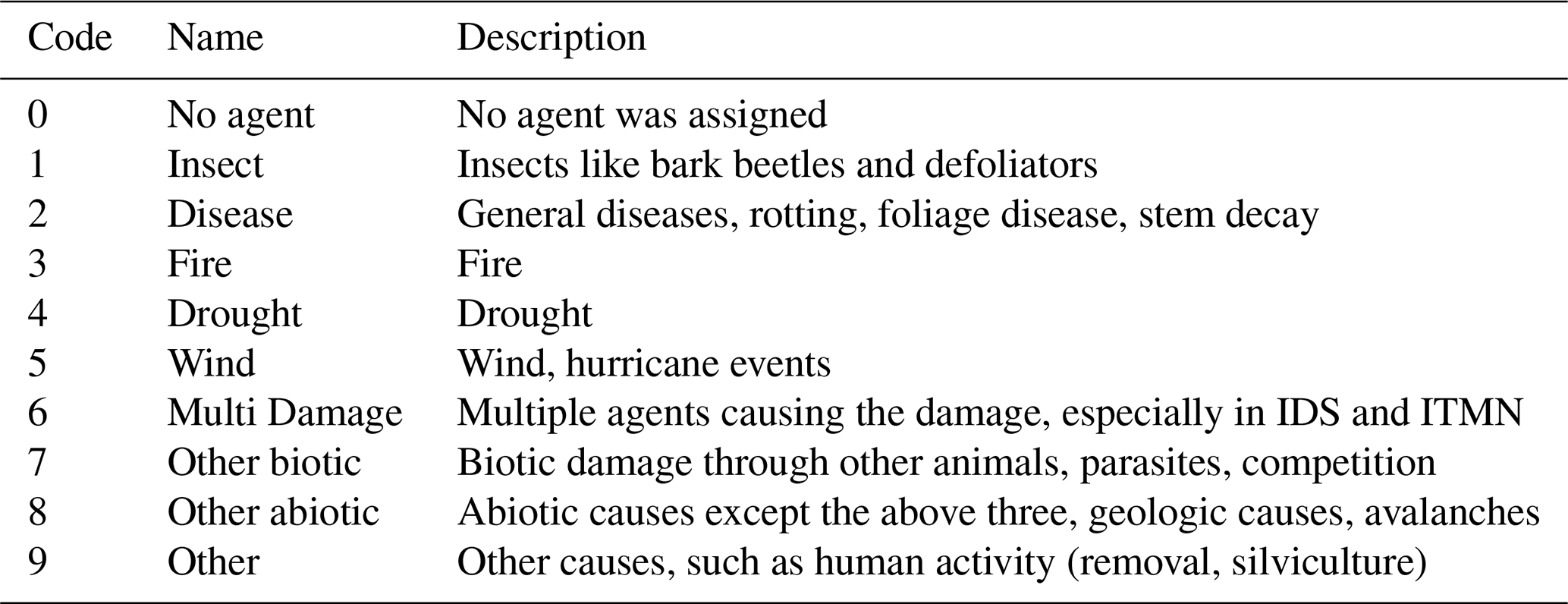
To enable consistent comparison of disturbance causing agents (DCAs) across datasets, we grouped different disturbance types into a unified coding system. This standardized classification accommodates the varying levels of detail present in the original DCA data from FIA, IDS, and NAFD (see Tables S1, S5 and S6). In the case of ITMN, we manually assigned the agent information to each event. The harmonized scheme comprises nine major disturbance categories, as shown in Table 2. In this study, we focus on natural forest disturbances and classify them into separate, detailed categories, while grouping animal-related causes, human activities, and other non-natural drivers into the broader Other categories. Drought is retained as an individual disturbance category because it is explicitly reported as a cause of mortality in FIA, IDS and ITMN, even though it often contributes to mortality in combination with other agents (Allen et al., 2015). For FIA, the mapping between original agent codes and the new classification is provided in Table S5. IDS provides detailed information on disturbance agents, including both general agent types and, in some instances, species-level identification. The original IDS classification comprises 26 distinct agent categories. Their mapping to the unified coding scheme is presented in Table S2. The NAFD disturbance types are similarly mapped to the new coding scheme, with the correspondence outlined in Table S6.
Table 2Coding system for major disturbance agent groups used in this study. The individual classes for each dataset are given in Tables S1, S5 and S6.
3.1.2 FIA
The FIA data includes information on different levels, like location, tree, plot, invasive species, ground cover and down woody material. Each level contains multiple database tables in csv format per state with detailed information for example about the condition, tree biomass, the plots itself. In this study, the Tree, Plot and Condition tables per state were used. The three tables are merged based on the plot sequence number, which is a unique number to identify a plot record, reported in each database table. The data is subset to only include forest land (COND_STATUS_CD == 1). The condition codes distinguish accessible forest (1), non-forest land (2), water bodies (3–4), and unsampled areas that may include forest (5). To ensure that only confirmed forest land with at least 10 % canopy cover by live tree species is included, we restrict the analysis to condition code 1. In some cases, multiple records correspond to the same disturbance event; therefore, the data is aggregated according to the plot sequence number, the disturbance agent, and the year of mortality.
The FIA data is provided as georeferenced point data, but the method of “fuzzing and swapping” due to privacy regulations described in Sect. 2.2 creates uncertainties to the locations of the plots. Therefore, we apply two buffer sizes – 800 and 1600 m – representing the 0.5 and 1 mile fuzzing radii, to account for possible uncertainties regarding the location precision when comparing with other datasets.
3.1.3 ITMN
The ITMN dataset is compiled from records of tree mortality attributed primarily to drought and heat in the literature and based on data requests (Hammond et al., 2022). However, tree mortality is a complex process, often caused by multiple factors which can, themselves be influenced by drought and heat (Allen et al., 2015). For example, biotic disturbances can benefit from heat and water stress, so that defoliator or bark-beetle outbreaks tend to occur during or following drought events (Allen et al., 2015). Such interactions between disturbances need to be considered when comparing with other datasets. To address this, we reviewed all publications in the ITMN dataset that document tree mortality in the USA to identify other possible disturbance agents. Specifically, we searched for additional disturbance agents reported in each original publication, and added this layer of information following our developed IDS coding system Table 2. Our compilation of disturbance agents based on the original literature from ITMN includes main three classes, namely Insects, Drought, and Multi damage. Since the ITMN data is point-based, two buffers of 500 and 1000 m were applied around the points to account for potential inaccuracies when comparing with other datasets.
3.1.4 IDS
The IDS data contain many different levels of information, including disturbance (type, intensity, percent affected), stand (tree species) and measurement details (survey year, month). The raw data table structured each event as a separate polygon with additional layers of information.
In some regions, IDS includes polygon shapes encompassing extensive non-forest areas and covering unrealistically large extents that seem to follow administrative borders (see Fig. A1). To address this, the area of each polygon is calculated and those exceeding a threshold of 2000 km2 are excluded. The data is dissolved based on identical survey years and disturbance agents to create multipolygons recording the same year and agent. Additionally, IDS includes various disturbance intensities, such as defoliation, topkill, and mortality. To ensure better compatibility with the other datasets, which are limited to reporting tree mortality, IDS data is filtered to include only mortality events.
3.2 Spatial comparison
We perform a pair-wise comparison on disturbed patches between each group of datasets, to compare the spatial agreement between the different datasets. In the point-based comparisons, a buffer is added to FIA and ITMN, further treating them as polygons, allowing for direct intersection with the polygonal records in IDS. For comparisons with the raster-based datasets (GFC and NAFD), raster pixels located within the buffered FIA or ITMN areas are extracted. The most common mortality year among these pixels is assigned as the representative disturbance year of the GFC and NAFD. In the case of NAFD, the associated disturbance type is also recorded. Spatially explicit comparisons follow a similar procedure, where the spatial overlap between each disturbed patch is calculated. We calculate the total number of disturbance events across CONUS for each dataset, along with the number of unique events identified in each pairwise comparison. For the spatially explicit datasets, we additionally compute the proportion of each individual disturbance patch that overlaps with another dataset. This allows us to assess both the overall spatial agreement and the correspondence in disturbance size and extent at the patch level.
3.3 Temporal comparison
We calculate the temporal lag between datasets as the difference between the recorded mortality years in each pair. A lag value of zero indicates perfect temporal agreement between datasets. Further, we analyse the temporal differences in disturbance date between datasets by fitting Gaussian Probability Density Functions (PDFs) to the time lags across overlapping pairs for individual events. The mean difference in mortality year detection between the two datasets provides an indication of potential systematic biases, while the standard deviation provides insight into the dispersion or variability in detection timing.
Understanding sources of disagreement is important to evaluate how uncertainties relating to dataset-specific characteristics might affect their applicability to certain problems. Here, we analyse the influence of FIA aspects contributing to uncertainty, namely land ownership, the timing and potential differences across states of data collection and reporting. We compare the differences in disturbance timing between FIA and the three spatially explicit datasets–IDS, GFC and NAFD. The distributions of temporal lags are assessed for different sub-sets of the data: (i) events in public and privately-owned land reported by FIA, (ii) events in FIA with coincident inventory/measurement and mortality year, and events where these do not coincide, (iii) events in different states. Additionally, temporal disagreement with remote-sensing datasets (GFC and NAFD) can also be due to limitations of disturbance detection due to topographic effects.
3.4 Disturbance agent comparison
We evaluate the agreement of disturbance-causing agent (DCA) classifications from IDS with those reported in FIA, ITMN, and NAFD for spatially and temporally overlapping events. Specifically, for each DCA category recorded in IDS, we evaluated the corresponding category assigned in the comparison datasets. We perform the analysis at the state level, reporting the accuracy metric as the proportion of direct matches between disturbance agent codes in each state. Additionally, we summarize DCA agreement across CONUS in a confusion matrix, using IDS as the reference dataset. The resulting heatmaps illustrate how frequently each IDS-assigned DCA category corresponds to classifications in the comparison datasets, with values normalized by IDS categories. Each row represents the proportional distribution of an IDS class across the comparison classes. In FIA, 42 % (811 951 events) of overlapping events within the study period lack reported agent information. We exclude these cases from the analysis, as they do not allow for categorical comparison. We also exclude Utah, since all overlapping events in this state occur after 2010, which is beyond the study period. FIA reports on wind and drought, but all 3423 wind events and all 7513 drought events lack the reported mortality year. Because this increases the uncertainty of timing and these events could appear outside the respected study period, they are excluded in the analysis.
3.5 Uncertainty modelling
Based on the previous analysis of temporal lags for FIA, the contribution of different uncertainty factors to the temporal lags with other datasets are analysed, specifically: ownership status (ownership), timing of inventory/measurement relative to reported mortality (meas_lag), administrative differences in data collection, in this case per state. These factors can affect the detection timing, but also might result in accuracy errors, which are then reflected in temporal lags in co-located disturbances. To quantify the effect of these variables on the temporal lags with FIA, a set of linear mixed effects models with the above mentioned factors as predictors are considered. For each pair of datasets, we fit a set of models in a step-wise manner with increasing number of predictors. We compare the models using an AIC-based comparison implemented in the ANOVA function of the lme4 package in R, and select the best-performing model based on these comparisons. The models follow the general equation:
where L corresponds to the temporal lag between each dataset pair (FIA–IDS, FIA–GFC, FIA–NAFD, shown in Fig. 4), β0 corresponds to the mean lag, with bO, bS and bD random effects contributing to the intercept: ownership, state and DCA, respectively. The interaction between ownership and state is included to account for state-dependent differences in the sampling of private vs. public plots. β1,i () are coefficients for the two variables considered as fixed effects (X, with size 2×n): elevation and meas_lag. The term ϵ corresponds to the residuals. Models with different numbers of random effects (1–4) and their combinations are fit to the data. Then, models with both fixed and random effects, including all combinations of 1–2 fixed effects (elevation and meas_lag) and random effects (State, ownership, DCA) are fit. Afterwards, all models are compared through ANOVA and the best model is selected as the one with the lowest AIC. Finally, the same procedure is repeated, but only for the sub-set of events where the measurement and the mortality year coincide, i.e. meas_lag is zero.
3.6 Trend analysis
We conduct a case study analysing disturbance trends across the western and eastern United States (West and East) from 2001 to 2010, with the aim of identifying regional patterns and differences among datasets. The West includes the states of Washington, Oregon, California, Idaho, Montana, Wyoming, Colorado, New Mexico, Arizona, Utah, and Nevada, while all other states are assigned to the East. We apply the non-parametric Mann–Kendall test (Mann, 1945; Kendall and Gibbons, 1990) along with Sen's slope estimator (Sen, 1968) to assess trend magnitude, direction, and statistical significance. To express the trend over the decade, we multiply the slope by 10, providing a decadal trend relative to the 10-year mean. We analyse both the number of disturbance events in all datasets and the total affected area (in hectares) for spatially explicit datasets. We compute overall trends for each dataset and region (West and East), considering the number of events for all five datasets and the total affected area for IDS, GFC, and NAFD. We then calculate trends by disturbance agent for FIA, IDS, and NAFD, comparing both event counts and, for IDS and NAFD, total affected area per agent and region.
4.1 Forest disturbance patterns in CONUS across datasets
The characteristics and differences of the datasets in terms of forest disturbance patterns in the CONUS region are summarized in Fig. 3. We excluded ITMN due to its limited number of recorded events. The figure highlights differences in temporal coverage, with FIA providing the longest record, spanning from 1957 to 2022. The datasets also differ in data format: FIA reports point-based counts of disturbance events, while IDS, GFC, and NAFD represent the spatial extent of disturbances. The figure also reveals notable differences in spatial coverage among the three spatially explicit datasets (IDS, NAFD, GFC). For the common period, IDS reports average disturbance extents that are 2–4 times larger than those captured by the remote-sensing products GFC and NAFD. The datasets show distinct temporal patterns in disturbance occurrence. Over the study period from 2001 to 2010, FIA shows a steady increase in the number of events, rising from about 96 000 in 2001 to 209 000 in 2010. IDS exhibits an initially high disturbed area (9.1 Mha in 2003), followed by a decline to a minimum of 6.1 Mha in 2005 and a subsequent increase to 9.6 Mha in 2009. NAFD remains relatively stable at approximately 3.6 Mha in the early years before decreasing to a minimum of 2.3 Mha, while GFC reports generally consistent disturbance extents with a mean of 1.9 Mha. Furthermore, for those datasets reporting disturbance agents, this first comparison already shows large differences, with IDS reporting predominantly insect disturbances (consistent with their mandate to survey insects and diseases) and FIA and NAFD reporting predominantly Other and Other Abiotic.
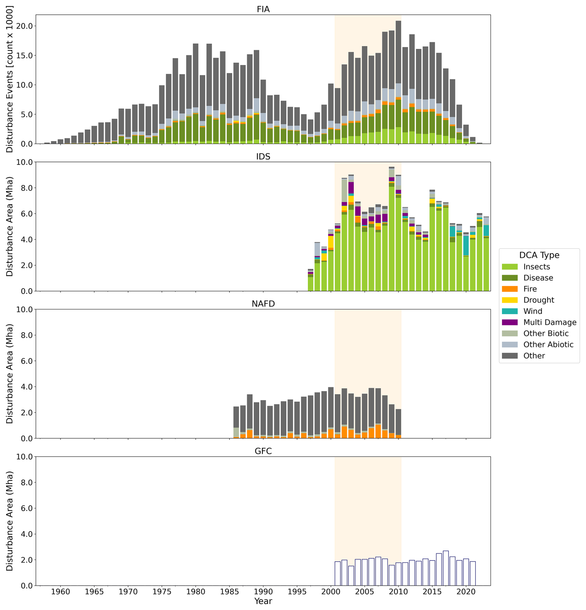
Figure 3Time series of disturbance records from the original datasets, showing event counts for FIA and disturbance area (in million hectares, Mha) for IDS, NAFD, and GFC. Where available, disturbances are categorized by DCA type; GFC data do not include this classification. The full temporal coverage of each dataset is displayed to illustrate their respective time ranges, with the study period from 2001 to 2010 highlighted. ITMN is excluded due to the limited number of disturbance events within the CONUS region. Note the differences in metric (event count vs. affected area).
Figure 1 further illustrates these differences within a focused subset region. In this area, FIA reports 249 disturbed plots, whereas ITMN records only 10 events. The subset area covers 3613.3 km2. Among the spatially explicit datasets, IDS detects 9782 disturbance events and maps the largest total affected area (4831.8 km2). Because in IDS disturbances can overlap, the total affected area can exceed the subset region area. GFC identifies 35 280 events, while NAFD reports the highest number of disturbances with 221 153 individual records – reflecting its finer spatial granularity compared to GFC. Despite the differences in event counts, GFC and NAFD both show similar spatial disturbance coverage, with 510.9 and 408.3 km2, respectively. However, NAFD has a higher number of smaller disturbance patches. Within the subset region, NAFD has a median patch area of 0.9 ha, with an interquartile range (IQR) of 0.0 ha. The median patch area of GFC is significantly larger, with 489.06 ha (IQR = 1477.3 ha), due to the aggregation method for GFC. IDS patches have a median area of 5.1 ha (IQR = 29.3 ha).
The total affected area per state and dataset (Fig. A2) also shows regional differences between the spatially explicit datasets. In general, GFC and NAFD have similar patterns, with lower disturbed area in the center of the USA and larger areas in the Southeast and West. IDS shows different pattern, especially in the West the affected area is the largest.
4.2 Spatial agreement
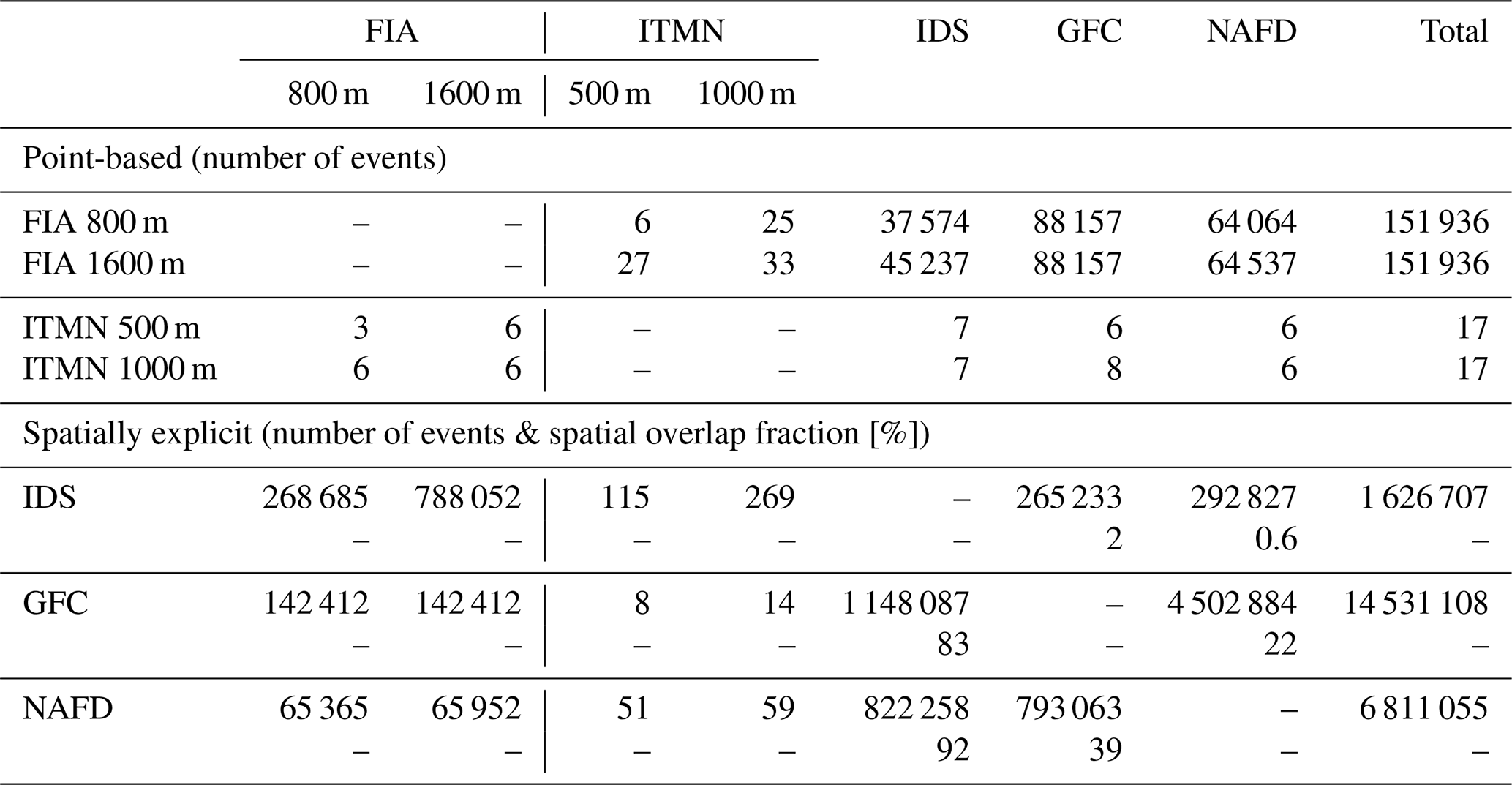
The distinct characteristics of each dataset and their proportional overlap in event counts and area are summarized in Table 3. Point‐based comparisons show moderate agreement between FIA and the spatially explicit products: around 25 %–30 % of FIA mortality events overlap with IDS, 58 % with GFC, and 42 % with NAFD (with larger buffers increasing the overlap slightly). In contrast, the overlap with ITMN is very limited due to the small number of monitored plots. For spatially explicit datasets, we compare: (i) the number of disturbed patches common to both datasets and (ii) the fraction of each individual disturbed patch in a given spatially explicit dataset that overlaps with another. IDS shares the largest number of its disturbance events with GFC, whereas GFC and NAFD show the strongest spatial overlap fraction with IDS (83 % and 92 % respectively). The spatial agreement between GFC and NAFD is rather low with 22 % and 39 % respectively. Contrary, only a small fraction of IDS area is shared with either product.
Table 3Unique overlapping disturbance events across all dataset comparisons. Point-based datasets are evaluated using different buffer sizes. For point-based datasets, the numbers indicate the total number of events per dataset overlapping with another. For spatially explicit datasets, the first row in each block reports the total number of overlapping disturbance events, while the second row gives the proportion of each dataset's disturbed area that overlaps with the dataset in the respective column (i.e., percentages refer to the dataset of that row). For example, among the overlapping events, only 2 % of the total IDS area overlaps with the GFC-affected area. The right column Total presents the total number of events from the original datasets in the study period.
4.3 Temporal agreement
The temporal agreement between dataset pairs, shown as Gaussian distributions of their mortality year differences, is presented in Fig. 4. The corresponding mean and standard deviation of each curve are given in the Table B1. The comparison between the two point-based datasets, FIA and ITMN, can be seen in the Fig. A3.
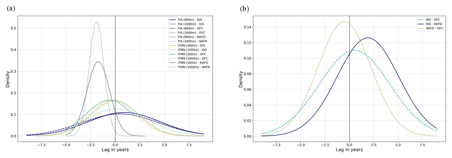
Figure 4Gaussian probability density function of differences in mortality years across CONUS for each pair of datasets, for the five datasets used in this study. The differences are analysed separately for pairs of point-based and spatially explicit datasets (a) and for pairs of spatially explicit datasets (b). Comparisons with the GFC data are represented as dashed lines, comparisons with IDS as solid lines. Negative values indicate an earlier disturbance detection of the dataset which stands first, compared to the second one. The values of the mean and standard deviation can be found in Table B1.
The comparison of FIA with the spatially explicit datasets (Fig. 4a) shows that FIA tends to report disturbances on average 0.7 years later than IDS and 0.5 years later than GFC and NAFD, but with large spread across individual disturbed patches, with standard deviations of 3.7 years for IDS and 3.9 years for GFC and NAFD. The larger buffer size does not reduce the lag between FIA and the other datasets, and increases slightly the lag with IDS (0.8 years). In contrast, ITMN (500 m buffer) reports disturbances earlier than the spatially explicit datasets – 0.1, 0.6, and 1.7 years earlier than IDS, GFC, and NAFD, respectively – with standard deviations of 2.4 years (IDS and GFC) and 1.2 years (NAFD). Increasing the buffer size results in larger mean lags with IDS and NAFD (differences of −0.4 and −1.9 years, respectively), but better agreement with GFC (differences of 0.1 years on average). The standard deviation in disturbance timing increases with buffer size for GFC and decreases for NAFD, but it is worth noting the small number of overlapping events for each dataset (Table 3).
The comparison between FIA and ITMN (Fig. A3) shows that FIA reports disturbances later than ITMN, with an average lag of 1.3 years for the 800 m (FIA) and 500 m (ITMN) buffers. Temporal agreement improves with larger buffers: using a 1000 m buffer for ITMN reduces the lag to 0.3 years, and increasing the FIA buffer to 1600 m yields a lag of 0.4 years. When both larger buffers are applied simultaneously, the mean lag decreases to 0.2 years with the lowest standard deviation (2.3 years). However, these results are based on small sample sizes: only 6 overlapping events for FIA and 3 for ITMN at the smaller buffers, and even at the largest buffers, overlaps remain limited (33 for FIA and 6 for ITMN, see Table 3).
Among the spatially explicit datasets, IDS generally records disturbances later than the satellite-based datasets, with average delays of 0.5 years compared to GFC and 1.9 years compared to NAFD. In both cases, the temporal uncertainty across individual patches remains high, with standard deviations of ±3.7 and ±3.2 years for IDS–GFC and IDS–NAFD. The two remote sensing datasets have a smaller spread of ±2.9 years and notably a negative mean lag of −0.5, indicating that NAFD detects disturbances earlier than GFC (Table B1). Across all datasets, the remote sensing datasets tend to detect disturbances earlier than the other datasets on average, except for the few events overlapping with ITMN, although with large temporal uncertainty across individual events (3–4 years).
4.4 Disturbance agents
Next, we compare the agreement between datasets in terms of their reported disturbance agent for FIA, ITMN, IDS and NAFD for the CONUS region and per state. Figure 5 shows results for IDS–FIA and IDS–NAFD, the comparison of IDS–ITMN is shown in Appendix A (Fig. A4), given the small number of samples for comparison. Since GFC does not report causes of tree loss, it is not included in this analysis.
In general, agreement between IDS and FIA tends to be higher in the western CONUS (26 %–52 %, excluding California with 14 %), and lower in the South and Northeast (0 %–22 %), reflecting the proportion of overlapping events where both datasets assign the same disturbance agent, see Fig. 5a). The highest agreement between the two datasets is found in Montana, with 52 % of overlapping disturbances sharing the same DCA, mostly due to good agreement on insect disturbances (53 %, Fig. A5). For CONUS, the DCA categories with the highest agreement between IDS and FIA are Insects (37 %), Disease (36 %) and Other (37 %), as shown by the confusion matrix (Fig. 5a). However, Insect events in IDS are frequently labeled as Disease in FIA (27 %), possible explaining the low consistency between datasets. Furthermore, there is greater spatial variability in the agreement between the two datasets for these disturbance types, with generally higher agreement in the western states for Insects and Disease, and higher agreement in the Other category for the midwestern states (Fig. A5). The category Multi-damage in IDS corresponds primarily to Insects and Disease in FIA (36 % and 37 %, respectively). The agreement for Fire and Other Biotic events is relatively low, 26 % and 32 % respectively, and with variable agreement across states (0 %–53 % and 0 %–100 %, respectively), without a clear spatial pattern. Drought events in IDS are often classified as Insects (34 %) or Other (20 %), even though FIA includes a drought category. However, this category was excluded from our analysis because FIA does not report a specific mortality year. Similarly, wind disturbances identified by IDS tend to be classified as Other (46 %) or Other Abiotic (29 %) in FIA, but are also omitted here for the same reason – lack of associated mortality year data.
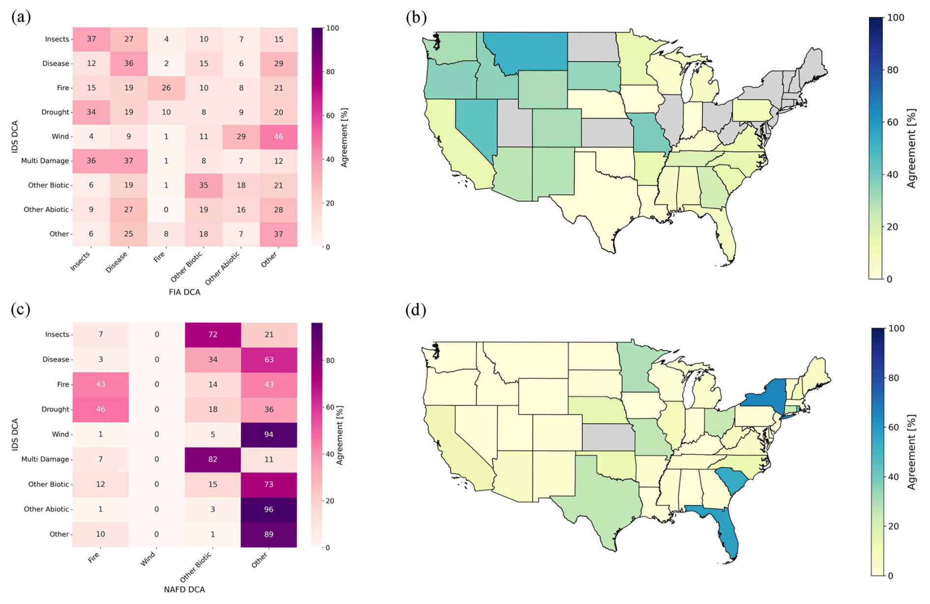
Figure 5Comparison of disturbance agent agreement between IDS and other datasets. Panels (a) and (c) show heatmaps of agreement matrices for IDS–FIA and IDS–NAFD, respectively, indicating how often each IDS-assigned disturbance agent category corresponds to classifications in the comparison datasets. Panels (b) and (d) display the corresponding agreement per state for IDS–FIA and IDS–NAFD. States shown in grey indicate no overlap between the respective datasets during the comparison period for events with identified disturbance agents. Heatmap values are rounded to integers; zeros may still correspond to very small overlaps.
NAFD shows higher spatial agreement with IDS in the southern and northeastern states (Fig. 5d). The highest agreement is found in New York State, with 66 % of overlapping disturbances sharing the same DCA, mostly due to the agreement on Other (100 %, Fig. A6). The NAFD uses a limited set of DCA categories – namely Fire, Wind, Other Biotic, and Other, broader than the ones provided by IDS. Figure 5c shows the heatmap of disturbance agent agreement between the two datasets. Insect disturbances in IDS are predominantly classified as Other Biotic in NAFD (72 %), while Disease tend to be attributed to Other (63 %), followed by Other Biotic (34 %) in NAFD. Fire events in IDS are either identified as Fire (43 %) or Other (43 %) in NAFD. Drought events reported IDS tend to be classified as Fire in NAFD (46 %), followed by Other (36 %). By contrast, Wind shows very low agreement, with 94 % of the wind disturbances recorded in IDS labeled as Other in NAFD instead. Table B4 shows that, from the NAFD perspective, most wind events coincide with IDS wind detections (56 %). However, these overlapping events represent only a small fraction of all wind disturbances recorded in IDS (0.36 %). Similarly, Other Biotic events in IDS are predominantly classified as Other in NAFD (73 %). The Other category shows high mutual agreement between datasets, with 89 % of events labeled as Other in IDS also categorized as such in NAFD. The agreement for disturbance types in NAFD varies regionally, with a strong spatial agreement for the Other category predominantly in the eastern and southern United States (52 %–100 %). Contrary, Fire and Other Biotic show higher agreement in the western regions (9 %–82 % and 13 %–100 % respectively).
Overlapping disturbance events between IDS and ITMN are found in only five states (Fig. A4). In Montana, all four overlapping events show 100 % agreement between the datasets, which attribute the disturbances to Insect agents. In Arizona, two overlapping events, reported as Insects and Drought in IDS and as Drought in ITMN, result in a 50 % agreement.
4.5 Sources of uncertainty
4.5.1 Ownership and timing records
First, the effect of data collection in privately-owned vs. public forests on the agreement between FIA with IDS, GFC and NAFD (Fig. 6a and Table B2), is analysed. Therefore, the comparison results with small buffer of 800 m are used, because of better results in the overall comparison (see Fig. 4 and Table B1). In the study period (2001 to 2010) the share is 64 % (100 620 plots) to 36 % (57 613 plots) of private and public plots in FIA respectively. In the FIA events overlapping with IDS, a total of 268 685 events were recorded, with 37 204 (14 %) occurring in privately owned plots and 231 481 (86 %) in public plots. We find that public forests tend to show similar differences in the reported timing of disturbance, than privately owned forests, with mean differences of 0.8 and 1.0 years respectively, which is similar to the temporal agreement overall without separating private and public plots (as analysed in Sect. 4.3). The uncertainty for both categories is around ±4 years.
In contrast, comparisons of FIA with GFC and NAFD reveal a pattern opposite to that observed with IDS and to the overall distribution in the FIA dataset. The majority of overlapping events occur on privately owned plots, accounting for 63 % in GFC and 66 % in NAFD. Within these private plots, the mean lag is relatively low, at 0.3 years for both GFC and NAFD, respectively. This lag increases in public forests, reaching a mean of 0.8 and 0.9 years for GFC and NAFD, respectively. The standard deviations are comparable to those observed in the FIA and IDS comparisons, as well as the overall comparison in Sect. 4.3, with approximately ±4 years. A per-state comparison of lags for private and public forests (Figs. A7, A8, A9) shows generally consistent patterns across the US, but also highlights state-specific differences and a clear contrast in the magnitude of timing differences between the western and central–eastern states.
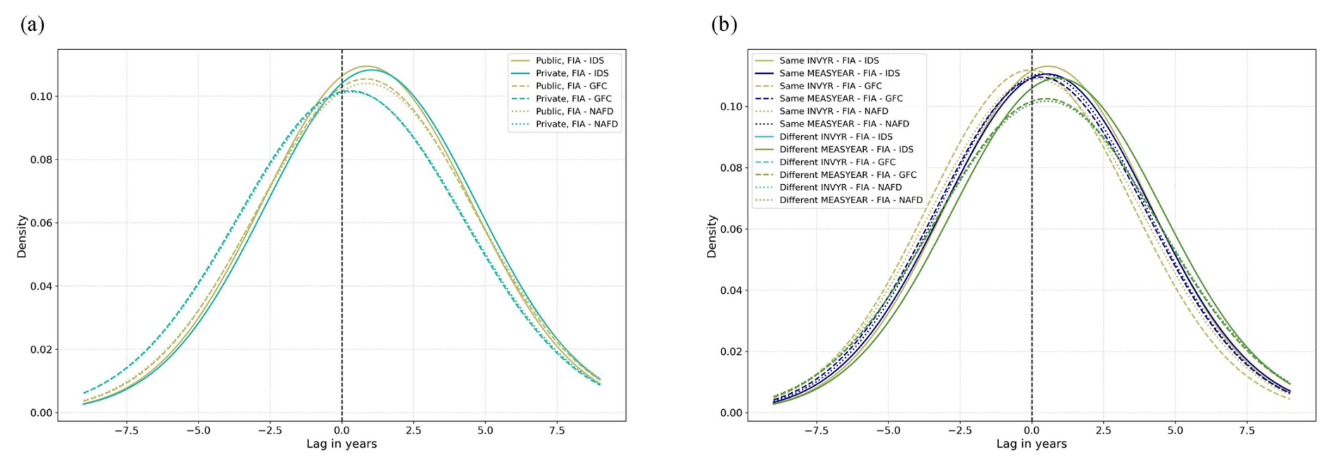
Figure 6Gaussian probability density functions of differences in reported mortality years (lag) across CONUS, used for uncertainty analysis. Comparisons involve FIA against IDS, GFC, and NAFD. ITMN is excluded due to the low number of overlapping events. Line styles represent dataset pairs: solid for FIA–IDS, dashed for FIA–GFC, and dotted for FIA–NAFD. Panel (a) illustrates the effect of FIA ownership class on temporal lag, with public forests shown in light khaki and private forests in cyan. Panel (b) shows the influence of different FIA timing records relative to the reported mortality year. Light khaki and navy indicate cases where inventory and measurement years match the mortality year; khaki and cyan represent cases with differing timing records.
Four distinct groups of FIA timing measurements are considered, based on whether the recorded mortality year aligns with the inventory or measurement year. The resulting differences in disturbance timing between FIA and the IDS, GFC, and NAFD datasets are analysed and presented in Fig. 6b. In Appendix B, Table B3 presents the classification of events based on whether the timing of recorded disturbances is the same or different across the three datasets, along with the corresponding mean lag, uncertainty, and the proportion of events in each category. Disturbances recorded in the same year exhibit a smaller mean lag compared to those recorded in different years, as well as compared to the overall mean lag reported in Sect. 4.3. The lowest mean lag, 0.0 years, occurs for overlapping events between FIA and GFC when the mortality year matches the inventory year in FIA. Despite this close alignment, all same-year events still exhibit an uncertainty of approximately ±4 years, consistent with the previous comparisons shown in Tables B1 and B2. Overall, when FIA reports mortality in the same year as the inventory and measurement, agreement with the spatially explicit datasets improves. However, such cases are relatively rare – only 2 %–4 % of overlapping events fall into the same-year category. In most cases, discrepancies among the mortality, inventory, and measurement years increase the mean lag and slightly raise the uncertainty. Nevertheless, both the mean lag and standard deviation remain comparable to the overall results.
4.5.2 Statistical analysis of temporal lags
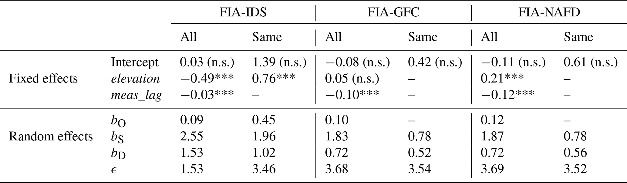
We analyse the uncertainty factors contributing to the spread in temporal differences between FIA and other datasets using linear mixed effects models (Table 4). For all three pairs of data, the best model explaining the temporal lag to FIA corresponds to the model with two fixed effects (difference between measurement and mortality year (meas_lag) and elevation) and the three individual random effects with no interaction term (ownership, state, DCA).
The best fitting model in all overlapping patches (“All” in Table 4) is the same for all three pairs of data (FIA–IDS, FIA–GFC, FIA–NAFD), including both elevation and meas_lag as fixed effects and all three random effects considered. The meas_lag coefficients are statistically significant for all three groups, with negative values for FIA–GFC and FIA–NAFD (−0.10 and −0.12, respectively), and small positive values for FIA-IDS. Negative coefficients indicate that the later the measurement year occurs compared to the reported mortality year, the more negative (earlier) is the lag between FIA and GFC. For elevation, the coefficients are positive and statistically significant in the FIA–IDS and FIA-NAFD comparisons. This suggests that, with increasing elevation, FIA reports mortality events earlier than IDS (by 0.49 yr km−1) and later than NAFD (by 0.21 yr km−1). In contrast, the effect of elevation is not statistically significant in the FIA–GFC comparison. In all three groups of data, the intercept is small and non-significant, indicating that on average the mismatches between the datasets are negligible. However, the residuals are generally large, between 1.5 to 3.7 years (consistent with the large standard deviation in the mean differences shown in Fig. 4 and Table B1). Random variability across states (bS) contributes the most to the variability in the intercept (2.55, 1.83 and 1.87 years for FIA–IDS, FIA–GFC and FIA–NAFD, respectively), followed by variability due to different disturbance agents (bD). Ownership status has a small contribution to variability in the intercept.
Given that measurement lag contributes significantly to the mismatch between FIA and the other datasets, a second model is fit only for those events where the measurement and the mortality year reported by FIA coincide (“Same” in Table 4). This allows to control for the influence of the revisit time to the disagreement between datasets. According to the corresponding best fitting models, elevation is only identified as a relevant predictor for FIA–IDS, with coefficients indicating that FIA reports mortality events 0.76 years earlier (coefficient −0.76) than IDS, per km of elevation. For the two satellite-based datasets, only random effects from state and disturbance type (DCA) are identified as relevant, the former contributing more to the variability of the intercept than the latter. While state is here considered as contributing to random variability in the intercept, Figs. A10, A11 and A12 show an apparent west-east difference in mean temporal lag, particularly for plots where the mortality and measurement years differ. The observed pattern may help explain why elevation emerged as a relevant fixed effect, despite non-significant coefficients in some comparisons. The results are consistent with analysis of the distributions of temporal differences earlier, indicating a small effect of ownership status on the mismatch between datasets.
Table 4Results of the linear mixed effects model fit for FIA–IDS, FIA–GFC, FIA-NAFD based on the step-wise model selection for all disturbed patches (“All”) and for disturbed patches where the measurement and mortality year reported by FIA are the same (“Same”). βelevation and βmeas_lag indicate the coefficients of the two fixed effects variables. The stars indicate significance values of the fixed effect coefficients (*** p<0.001, ** p<0.01, * p<0.05, n.s. p>0.05). bO, bS and bD indicate the standard deviation in the intercept associated with random effects from ownership, state and DCA, respectively. In some cases, the best model includes fewer variables than the ones shown, in that case, the model corresponds to the values shown. For example, for the FIA-GFC model for “Same”, the best model includes only random effects for state and DCA.
4.6 Trends across CONUS
The trends in event numbers for each dataset and region are shown in Fig. 7. Disturbance event counts differ across datasets and between the East and West. In the West, the two point-based datasets (FIA and ITMN) show increasing event counts, consistent with the positive trend observed in IDS. Contrary, GFC and NAFD indicate decreases in the West, with NAFD showing a significant decline of −105 %. Trends in the East are less pronounced: IDS reports an increase of +76 % relative to the decadal mean, while FIA does not exhibit a detectable trend in this region. In contrast, NAFD again shows a significant negative trend (−33 %), and GFC shows only a slight decrease.

Figure 7Trend in disturbance event numbers by region. Rows correspond to datasets and columns to regions in the US (West and East). Positive values show increasing trends relative to the decadal mean. Asterisks denote significance levels (***: p<0.001; **: p<0.01; *: p<0.1). Grey boxes indicate insufficient data to calculate a trend.
Similar patterns appear in the trends of total affected area (Fig. A13). In the West, IDS shows a positive trend (+72 %), while GFC and NAFD indicate non-significant decreases in disturbed area of −30 % and −68 %, respectively. In the East, IDS shows the strongest decline (−130 %), followed by NAFD with a non-significant decrease of −20 %, and GFC exhibits a slight negative trend (−10 %).
To further investigate differences in disturbance dynamics, we also analyse trends by disturbance agent (Fig. 8). ITMN is excluded from this assessment due to the low number of reported events. In the West, NAFD shows predominantly decreasing trends across the three agents present (Fire, Other Biotic, and Other). In contrast, FIA reports increases for the reported agents, with all trends highly significant except for Fire. Drought, Wind, and Multi Damage are not represented in FIA. IDS exhibits a similar pattern to FIA, but with lower magnitudes and fewer significant trends. Drought and Fire are the only agents with a decreasing trend in the West in the IDS dataset. Patterns in the East differ both among datasets and compared to the West. FIA shows significant increasing trends for Insects (+42 %), Disease (+56 %), and Fire (+79 %) relative to the decadal mean. IDS follows the overall directional pattern seen in the West. NAFD shows widespread declines across agents in the East, except for Fire, which exhibits a strong increase of +157 %. Wind disturbances occur only in the East in NAFD, with a non-significant decline over the decade.
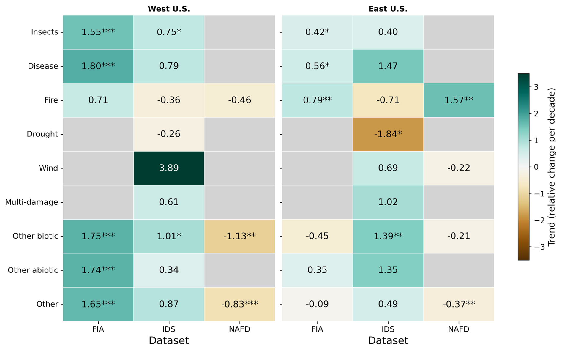
Figure 8Trend in disturbance event numbers per region and disturbance agent. Asterisks indicate significance levels (***: p<0.001; **: p<0.01; *: p<0.1). Rows represent datasets and columns represent regions (West and East). Positive values indicate increasing trends relative to the decadal mean. Grey boxes indicate insufficient data to compute a trend.
We observe similar patterns when examining trends in total disturbed area by agent (Fig. A14). In the West, IDS shows mixed responses across disturbance agents: only Insects, and Other Biotic disturbances show increasing affected area, Multi Damage exhibits no trend, all other agents show decreasing trends. In the East, IDS largely indicates declining disturbance areas, with only Other showing increases. NAFD reveals patterns largely consistent with the event‐based trends. In the West, all agents show declines in disturbed area, whereas in the East, Fire stands out with a substantial increase of 141 % relative to the mean. The remaining three agents (Wind, Other Biotic, and Other) show reductions in affected area over the decade.
Forest disturbances have multiple causes and affect forests in varied ways, shaping how they can be observed and interpreted. Some agents, such as windstorms, cause abrupt structural damage (Forzieri et al., 2020), while others, such as insects or drought, may act more gradually or interactively, altering forest composition, vitality, and recovery potential (Meddens et al., 2012; Kurz et al., 2008; Clark et al., 2016). These differing disturbance mechanisms influence not only their ecological consequences but also how readily they can be detected, attributed, and quantified in observational datasets.
Overall, we observe a relatively good average agreement (i.e. good accuracy) among the datasets in terms of disturbance timing and agents, but with considerable variability across individual events (i.e., low precision). The spatial agreement is generally lower: while IDS captures most of the area detected by the two remote sensing datasets, only a small fraction of IDS area – at most 2 % – overlaps with the remote sensing products. Between the remote sensing datasets themselves, spatial agreement is only moderate. The results show that differences between the datasets can be attributed to inherent uncertainties in detection methods, differences in spatial and temporal scales, and varying levels of detail in the disturbance records of each dataset. Below, we discuss how the uncertainties underlying the different datasets explain these mismatches, and provide guidance for users on how these differences might affect analyses and interpretations.
5.1 Methodological uncertainty
A number of methodological uncertainties arise from the way the data is collected and from the algorithms used to detect and characterize disturbances. Both FIA and IDS are used for systematic monitoring of forest disturbances, but they differ in scale and methodology. The FIA is distributed across the whole CONUS region, but is based on small (<10 m) plots which are revisited typically every 5 or 10 years (Schroeder et al., 2014). Aerial surveys in IDS provide large-scale information as disturbance polygons, but typically focus on regions where outbreaks have been known to occur. Although effective in capturing major disturbance and mortality events, the IDS may miss disturbances in remote, unmanaged forests, and urban areas (Kautz et al., 2017). Additionally, aerial surveys face inherent limitations in detecting slow-acting or long-term disturbances and in distinguishing the primary cause of mortality in complex compound disturbance scenarios (McDowell et al., 2015). The subjectivity of hand-drawn disturbance polygons further affects data quality, particularly in IDS Regions 8 and 9, where some polygons cover unusually large or irregular areas, including urban zones (see Fig. A1). These inaccuracies affect spatial comparisons and analyses, potentially leading to erroneous results and differences in spatial agreement (Fig. A2, Table 3). This could be improved through post-processing. Comparing the data with higher-resolution remote-sensing products – such as Sentinel-2 or PlanetScope imagery or detailed tree-cover maps – could help reduce spatial uncertainty (Coops et al., 2023; Müller et al., 2025).
The ITMN data is recognized to be inherently biased due to the use of literature-based reports of tree mortality in the field (Hammond et al., 2022). As a result, some regions and forest types are underrepresented. In the US, for example, only 17 unique mortality events were reported between 2001 and 2010 (Table 3). In addition, the point-based format introduces uncertainty in the precise location and spatial extent of each event. Reported mortality can range from single points to dense clusters, reflecting substantial variation in event size and making spatial interpretation challenging.
Satellite data allows for spatially and temporally continuous disturbance mapping, but the detection of a given disturbance inherently depends on its size, as satellites operate with varying spatial resolutions. Both, the GFC and NAFD datasets are based on Landsat with a 30 m spatial resolution (Hansen et al., 2013; Schleeweis et al., 2020), so that smaller scale events might remain undetected (Masek et al., 2013; Cohen et al., 2016). For disturbances to be detected, the signal must reach a detectable threshold for satellites to identify and quantify the affected area, which standardizes detection, but also makes disturbance severity a critical factor in satellite-based mapping (Masek et al., 2013; McDowell et al., 2015). Moreover, similar disturbances can manifest differently across ecosystem types, resulting in varying detection outcomes (Cohen et al., 2017).
The approaches used to determine forest disturbances differ notably between GFC and NAFD. In GFC, using the maximum annual NDVI decline (Sect. 2.5) can result in gradual or low-severity disturbances being missed or misclassified, leading to underestimation of forest loss (McDowell et al., 2015). Conversely, short-term fluctuations caused by phenological changes or sensor noise can be erroneously identified as loss events, even though they might be only temporary. Due to these issues, Hansen et al. (2013) highlight uncertainties associated with the GFC dataset and advise using a 3-year moving window to detect trends, cautioning for area estimation using pixel counts of forest loss. These methodological sensitivities help explain the temporal patterns observed in our comparison: GFC tends to register disturbances earlier than FIA and IDS, which rely on field-based inventories with coarser temporal resolution, but later than NAFD, reflecting differences in the underlying detection algorithms (see Fig. 4/Table B1). The relative timing reflects differences in how each dataset detects and defines disturbance events. In contrast, the NAFD algorithm uses a more complex modeling approach by applying Random Forest models (Sect. 2.6), which are well suited for capturing complex relationships between spectral features and disturbance types (Prasad et al., 2006). The combination of multiple decision trees increases accuracy and reduces overfitting as the ensemble grows (Prasad et al., 2006). In our temporal comparison, NAFD detects disturbances earlier than the other datasets – on average by about half a year (Figs. 4, B1). This could reflect the ability of the framework to capture subtle spectral changes preceding the disturbance detection by other approaches.
Additionally, disturbance events vary widely in both spatial extent – from several meters to hundreds of square kilometers – and temporal duration – from hours to multiple years (Turner, 2010), so that the suitability of each approach is also dependent on the disturbance characteristics. Methodological differences thus result in spatial and temporal uncertainties, which we discuss below.
5.2 Spatial uncertainty
In general, the spatial agreement of overlapping events is low. Differences of the spatially explicit datasets in terms of total affected area in Fig. A2 reveal substantial differences between IDS and the two remote sensing datasets GFC and NAFD. In IDS a strong East-West difference is shown with higher total affected area in the West US, maybe due to more extensive acquisition or because of more disturbances. This is also shown by an increasing trend in the west of IDS and a decreasing trend in the east (see Fig. A13). The patterns of GFC and NAFD are generally similar, and their overall trends are also comparable, showing a decreasing development across both regions (East–West) (Figs. A2, A13).
Overall, the spatial alignment among the disturbance datasets is low, reflecting fundamental differences in how each dataset defines, detects, and maps affected areas. Spatial uncertainty arises not only from methodological choices, but also from regional variation in data availability and disturbance characteristics. The strong contrasts visible in the total affected area across datasets (Fig. A2) highlight these discrepancies: IDS reports considerably larger disturbed areas in the western US than in the east, a pattern that may reflect both higher disturbance activity in this region and differences in acquisition intensity or mapping conventions. These regional differences are further shown in the opposing trends shown by IDS in Fig. A13, where disturbance area increases in the West but declines in the East. In contrast, GFC and NAFD, which rely on similar satellite imagery and automated detection approaches, tend to show more consistent spatial patterns with each other, both decreasing trends in both regions, demonstrating that satellite-based detection methods have a more consistent spatial footprint.
The per-patch comparison reveals a low average spatial overlap between IDS and the remote-sensing datasets GFC and NAFD, with 2 % and 0.6 % respectively. This is also visually evident in Fig. 1, where IDS polygons span large areas, whereas GFC and NAFD often detect disturbances as isolated single pixels (30 m × 30 m). The multi-layer structure of IDS, which can assign multiple disturbance agents or years to the same area, further expands its total disturbance extent and influences the spatial overlap metrics. Despite being derived from the same Landsat imagery, GFC and NAFD show only moderate agreement in disturbance extent, highlighting the impact of differing detection algorithms and classification strategies. As a US-specific product, NAFD is likely more reliable because it is trained with system specific training data points and employs a more specific algorithm that accounts for additional sources of noise and uncertainty. IDS may overestimate disturbance extent due to surveyor bias and manually drawn delineations, whereas remote sensing products may underestimate it because of their reliance on spectral signals and algorithmic limitations, as discussed above.
As an additional spatial uncertainty, the IDS inventory reports the total area affected by a type of disturbance agent, rather than the precise disturbed forest area (Meddens et al., 2012). Contrary, the FIA only reports point-based disturbances. Therefore, satellite imagery might more accurately detect and delineate the exact disturbed area (Meddens et al., 2012; Masek et al., 2013), providing a detailed spatial perspective.
5.3 Temporal uncertainty
Overall, the dataset comparisons reveal relatively small temporal discrepancies, with an average mean lag of approximately half a year (Table B1). The lowest mean lag and spread are found in comparisons involving ITMN (Figs. 4 and A3). However, these results are based on a limited number of overlapping events, reducing their statistical robustness and interpretability. FIA consistently reports disturbances later than the other datasets, as does IDS when compared to ITMN, GFC, and NAFD. These delays are likely due to their methodological uncertainties: both FIA and IDS are subject to irregular revisit intervals – up to 10 years in some cases (Schroeder et al., 2014; Cohen et al., 2016), which introduces variability in disturbance timing. However, IDS generally reports earlier than FIA, likely because it relies on aerial detection over broad areas, allowing for earlier identification of visible disturbance symptoms.
FIA depends on in-field plot measurements, which may only capture mortality when plots are resampled, often years after the actual disturbance occurred. Indeed, we find that temporal agreement of FIA with other datasets improves substantially when the mortality year aligns with both the inventory and measurement year, compared to events where the mortality year and the inventory or measurement year differ (Fig. 6/Table B3), highlighting the importance of accurate timing information. Furthermore, we find a difference between states when FIA mortality years differ from inventory and measurement years (Figs. A10, A11 and A12), which might be explained by accessibility challenges in high-elevation areas in the west, which can delay field measurements, while aerial or satellite-based datasets (IDS, GFC, NAFD) are less affected and therefore detect disturbances earlier. This pattern is also reflected in our model results for FIA, which show a strong association with elevation (Table 4). In situations where accessibility constrains field surveys, remote sensing data can help bridge this gap by providing consistent observations even in remote areas. While elevation and accessibility help explain broad regional differences in temporal alignment, we also investigated the effect of swapping and fuzzing in the FIA data. The FIA's guidelines suggest that swapping and fuzzing introduces only minimal differences in the data (Burrill et al., 2021). By testing ownership influence, our results show that, in the FIA–IDS comparison, privately owned plots exhibit a slightly larger spread in reported disturbance timing than publicly owned plots (Table B2). In contrast, for the FIA–GFC and FIA–NAFD comparisons, mean lags are lower on private lands than on public lands. This might be explained by the fact that disturbances on private lands – associated with active management or commercial logging – lead to more abrupt canopy changes. These processes may align more closely with remote-sensing disturbance detection than with the sampling schedule of ground-based inventories. Overall, the statistical model results support only a minor influence of ownership status on temporal agreement among datasets (Table 4), confirming that anonymization procedures in FIA do not meaningfully bias the spatial or temporal comparisons conducted here. However, the per-state visualizations (Figs. A7, A8, A9) show regional variation of ownership effects, suggesting that state-level factors, such as management practices, or methods in plot measurement, may have an influence on the observed temporal mismatches.
The Landsat-based disturbance datasets GFC and NAFD tend to detect disturbances earlier than FIA and IDS, likely due to their higher temporal resolution, as satellite overpasses occur more frequently than the revisiting intervals of ground-based inventories. Conversely, both GFC and NAFD detect disturbances later than ITMN. However, due to the limited number of overlapping events between ITMN and the other datasets this comparison is less robust. Direct comparisons between GFC and NAFD show strong overall alignment in disturbance timing, though NAFD tends to detect disturbances earlier or more readily than GFC. At the state level, agreement between GFC and NAFD varies depending on the disturbance agent classified by NAFD (Fig. A15). Human-activity classes (Removal and Conversion) show small lags, whereas other agents (Stress, Fire, Wind, and Other) exhibit larger timing differences, with differences across states. GFC captures abrupt canopy changes well, but reports later than NAFD for stress-related disturbances, which are more gradual and subtle, posing challenges for detection with NDVI-decline metrics. With the recommended use of a 3-year moving window for GFC (Sect. 5.1), the uncertainty introduced by the change-detection algorithm can contribute to the larger spread in timing differences observed between GFC and the other datasets. This highlights the influence of algorithmic differences despite both products relying on the same Landsat archive (see Sect. 5.1). While consistent, annual remote-sensing data support close temporal agreement, the remaining spread indicates that meaningful event-level differences in disturbance detection still persist.
Differences in revisit frequencies between inventory based and the remote-sensing datasets, and in the satellite detection algorithms, are likely to explain differences in disturbance trends across CONUS (Fig. 3) and in western and eastern US (Figs. 7 and A13). While inventory data report positive disturbance trends in 2001–2010 in both regions, remote-sensing datasets report predominantly negative trends, but less pronounced for GFC compared to NAFD. All datasets agree, however, on more pronounced trends in western US than eastern US, meaning that the disagreement in disturbance trends between inventory based and remote-sensing datasets is larger for the western US These differences are found across most disturbance agents (Fig. 7), so that the temporal uncertainty seems to be the predominant cause for this trend mismatch. We note however, that spatial uncertainty also likely plays a role, as shown in Figs. 1, A2, and Table 3.
5.4 Disturbance agents
Our results indicate moderate to low consistency of disturbance agent attribution across datasets, which can be explained by several factors. A key challenge is the prevalence of compound disturbances. For instance, drought stress can lead to bark beetle outbreaks and eventual mortality (Bentz et al., 2010; Seidl et al., 2017; Burton et al., 2020; Fettig et al., 2022). Such cascading effects make it difficult to attribute mortality to a single agent, and attribution can vary between datasets depending on how interactions are interpreted. This ambiguity is reflected in the moderate overlap of the IDS category Multi Damage with FIA (Fig. 5a). In the comparison with NAFD (Fig. 5c) Multi Damage disturbances in IDS mainly match Other Biotic in NAFD, referring to the original category Stress. This includes multiple possible drivers such as insects, drought, or disease. A similar pattern occurs for fire events: IDS may first record insect or disease disturbances, while subsequent canopy loss from fire is captured later in NAFD, contributing to low fire agreement between datasets. These results highlight that the prevalence of multi-damage disturbances, combined with differences in classification schemes across datasets – like IDS being focused on insect and disease surveys – makes assigning a single cause to forest damage inherently challenging. These thematic and structural differences emphasize the need for harmonized classification systems when integrating multi-source disturbance data.
The granularity of agent classification and temporal resolution also play critical roles. While FIA records disturbances such as drought and wind, many of these events lack assigned mortality years during the study period and were excluded from our analysis. This discrepancy likely reflects the limitations of field-based reporting and revisit times (see Sect. 5.3), where certain disturbance types, despite having predefined codes, may be under-reported or inconsistently documented due to their subtle impacts or challenges in attributing tree mortality to specific agents within a given time frame.
Differences in the reported agents could also arise from temporal lags in aerial surveys (see Sect. 5.3). If, for example, surveys are conducted after drought conditions subside, only subsequent biotic damage may be detected. Nevertheless, Coleman et al. (2018) showed that the detection of damage types and agents in IDS dataset could be improved by aligning flight conditions and timing with the biological windows of disturbance agents. However, they also noted that limited ground-truthing and the subjective nature of aerial surveys – affected by different surveyors, viewing conditions, and flying conditions – introduce variability and uncertainty into the data (Coleman et al., 2018; Meddens et al., 2012). In addition, aerial surveys face inherent limitations in detecting slow-acting or chronic disturbances and in discerning the primary cause of mortality in complex or compound disturbance events (McDowell et al., 2015). Addressing these limitations represents a key opportunity to improve disturbance monitoring methodologies in the future.
Remote-sensing technology is widely used in forest disturbance mapping (Banskota et al., 2014), but attribution to specific agents based on remote-sensing data only is still limited. While now being a standard approach to identifying certain types of disturbances like those caused by fire (Chuvieco et al., 2018, 2022; Otón et al., 2019), distinguishing other disturbances such as different biotic agents, and especially non-stand replacing ones is more challenging (Senf et al., 2020; Senf and Seidl, 2021b; Senf et al., 2017; McDowell et al., 2015). NAFD integrates agent attribution into its remote-sensing approach. While wind events only occur in the east of the US (see Figs. 8 and A14), Schleeweis et al. (2020) note that they had not enough wind events and conversion in the West of the USA as training data so they cannot generate accuracy metrics. This is reflected in Table B4, where the total number of wind events is markedly lower than for other disturbance agents. Similar methodological constraints apply to fire, which may contribute to the low agreement with IDS. Schleeweis et al. (2020) note that when multiple fires occur in a single pixel, only the highest magnitude (or most recent, if tied) event is retained, so this compositing approach likely underestimates sequential canopy loss. Additionally, producer accuracy for fire is higher in the West than in the East leading to regional differences. Other causes are broadly categorized as human activity or ambiguous classes like Stress, reflecting the limitations of remote sensing in distinguishing non-fire agents (Schleeweis et al., 2020). Thus, while NAFD offers valuable long-term information on disturbance dynamics, particularly for retrospective analyses, its capacity for detailed agent attribution is constrained by methodological limitations.
For ITMN, a detailed quantitative comparison was not feasible due to the low number of records and limited geographic scope. Although ITMN primarily reports drought-induced mortality, literature indicates that many of these events may involve compound disturbances, such as interactions between drought stress and bark beetle infestations. This suggests that some ITMN records classified under drought may, in reality, reflect Multi Damage phenomena, further complicating direct comparisons with datasets that separate agents more explicitly. Ad-hoc literature-based synthesis, as is the case of ITMN (Hammond et al., 2022), are prone to biases in terms of the key-words used to select relevant studies, as well as inconsistencies in the interpretation and granularity of driving agents reported in each individual study. Indeed, here we found a tendency towards higher attribution to drought-related disturbances in ITMN, in isolation or in combination with biotic agents, while IDS tended to associate mortality events mostly with bark beetle disturbance for the same events.
These factors collectively contribute to the observed low consistency in disturbance agent determination and underscore the challenges involved in accurately identifying and classifying forest disturbances. The discrepancies between datasets, the complexities of cascading disturbances, and the limitations of current detection methods all highlight the need for improved approaches in forest disturbance monitoring.
5.5 Recommendations
All five datasets evaluated in this study exhibit distinct characteristics, making them suitable for different research applications and analytical contexts.
Among the point-based datasets, FIA offers detailed long-term (1957–2022) disturbance information with broad agent categories across the United States. Its extensive temporal coverage and rich attribute data make it well-suited as a reference or validation dataset and for training machine learning models that require agent-specific information. However, its applicability for large-scale applications is limited by its point-based nature, inconsistent data availability across states, and irregular and low-frequency revisit intervals, which may pose challenges for certain modeling approaches. The results show an important influence of the inventory/measurement revisit timing on the uncertainty in the timing of mortality (Sect. 5.3) Ownership status shows a small contribution to the temporal mismatches, indicating that the fuzzing and swapping procedure allows to characterize well the disturbance occurrence, at least at the scales analysed here, although we note that regional differences can be larger (Figs. A7, A8, A9). Applications using FIA that require precise timing of the mortality event (e.g. to evaluate drivers, or develop predictive models) should limit the analysis to events with matching mortality and measurement/ inventory years to effectively reduce temporal uncertainty. While this reduces the number of samples, the broad spatial and temporal coverage of FIA data still allows for a very large number of samples. More frequent observations may enhance temporal and potentially spatial consistency across datasets, thereby reducing uncertainty. Given the uncertainty in reported years, studies using FIA to analyze disturbance agents should be aware that events recorded between inventory or measurement periods may have less precise timing especially for slow onset and more subtle disturbance agents, particularly in regions or plots with longer revisit intervals, which can affect interpretation of the sequence or cause of mortality.
ITMN, while also primarily inventory based, is a smaller, globally distributed dataset primarily capturing drought-related mortality. The dataset is known to be biased toward the Northern Hemisphere (Hammond et al., 2022) and lacks the spatial and thematic detail of FIA. Nevertheless, ITMN can serve as a valuable exploratory dataset or a complementary source in regions where detailed inventory data are unavailable. However, we note that ITMN predominantly attributes mortality to drought while in fact mortality might be driven by a combination of drought and biotic agents. Comparisons involving ITMN show the smallest standard deviations in temporal lags, however, it has small sample size, making it impossible to better understand sources of mismatches. While the general good temporal agreement makes ITMN valuable as a validation dataset for tree mortality occurrence, its small and potentially biased sample set limits its suitability for model training and further analyses. Furthermore, we recommend combining ITMN with other datasets to better identify mortality causes beyond drought.
Among the spatial datasets, IDS provides high-resolution polygon data with detailed agent attribution over the entire CONUS. This level of detail makes it particularly valuable for training models aimed at detecting and classifying disturbance agents. While it is primarily developed for insect and diseases, often reporting down to the species level, IDS includes a range of other relevant disturbance agents, in fact, covering the same broad categories as FIA and with additional detail (Table S1). In addition to mortality events, IDS also includes various damage categories like crown discoloration, topkill and dieback. Nevertheless, some limitations should be taken into account, namely its potential subjectivity in delineated disturbance areas due to human labeling, and limited revisit frequency. IDS is particularly well-suited for large-scale analyses of forest disturbance types, offering detailed agent attribution and spatially explicit polygons across CONUS. Its granularity and broad thematic coverage make it useful for model training and classification tasks. The high level of detail of IDS can also be used to refine detection and classification methods, e.g. by sub-sampling events based on disturbance severity, or type of impacts. However, given potential uncertainties from manual interpretation and limited revisit frequency, IDS is best used in combination with other datasets for robust temporal analyses or validation. Increasing survey revisit frequency could allow for better detection of slow declines or compound events, which are often missed with the current 5 to 10 year interval (Cohen et al., 2016; Schroeder et al., 2014).
GFC, a globally consistent and annually updated remote-sensing product, offers broad coverage of forest loss but lacks information on disturbance agents or severity. Notably, our analysis indicates that GFC detects disturbances earlier than the other datasets, underscoring the value of remotely-sensed imagery to identify disturbances. Furthermore, given its global coverage and long period (since 2001 and annually updated), GFC can be applied to large-scale trend analyses, change detection, forest change monitoring, as previous studies have shown (Hansen et al., 2013). Based on the results, GFC is shown to be very promising for timely mortality detection, which can help to improve understanding about drivers and develop predictive models. However, given that it does not include information about disturbance agents, it needs to be combined with other datasets, preferentially ground-based, e.g., as reference data. In that case though, careful consideration of the uncertainties underlying such additional datasets is needed.
NAFD provides agent-attributed disturbance information from 1986 to 2010 across the US, making it well-suited for retrospective studies and long-term trend validation. Although it lacks recent data, NAFD remains a valuable historical resource when integrated with more current datasets. In principle, the dataset could be extended to the present using annually updated Landsat imagery. To improve agent attribution, NAFD could be integrated with complementary ground-based or higher-resolution datasets, such as PlanetScope or Google Earth, that provide more precise information on disturbance type. Structural information from sensors like Sentinel-1 may further aid in distinguishing certain disturbance types (Müller et al., 2025).
Generally, the datasets show good agreement in disturbance timing. In principle, increasing the temporal resolution of the datasets, e.g. with revisits for different phenological stages, could support earlier and more timely detection of disturbances. However, despite the temporal agreement, spatial overlaps among datasets remain low, highlighting substantial divergence in the location and extent of disturbances. This discrepancy underscores the challenges in defining, detecting, and mapping forest disturbances consistently across datasets. However, increasing the temporal resolution of inventories is impractical and costly. Satellite-based datasets could bridge this gap. While trend break detection algorithms based on Landsat are likely to be limited to annual scale, new sensors such as the ones on board of the Sentinel constellation, with both high spatial and frequent revisit times, as well as global coverage, might allow for sub-annual disturbance detection.
Additionally, we find discrepancies between agent attribution and level of detail in inventory-based data. These limitations can further contribute to the mismatch with remote-sensing based data. Additional information about disturbance severity and specific impacts (e.g., leaf discoloration, legacy pattern, percent affected) are available for IDS and could in principle be added to regular forest inventories. This would allow to identify the most appropriate satellite dataset (optical, radar, etc) for each type of disturbance and associated impact, and possibly improve their detection regarding timing and spatial features.
In this study, we assessed the consistency of five forest disturbance datasets across the conterminous United States, highlighting the challenges of comparing and interpreting these data. Our results reveal varying levels of agreement, with the remote-sensing dataset generally reporting disturbances earlier than the others, underscoring the need for careful consideration of dataset differences when analyzing forest disturbance patterns.
Overall, the spatial agreement between datasets depends strongly on perspective. GFC and NAFD overlap substantially with IDS, but the multi-layered nature of IDS results in a small portion of its total area aligning with the other data. Comparisons with point-based FIA show moderate agreement, reflecting both differences in data type and sampling design.
In overlapping events, we find good temporal agreement in the mean reported mortality year across pairwise comparisons which ranges between 0.1 to 1.9 years. However, the temporal uncertainty varies between 1 and 4 years. Satellite-based datasets tend to identify disturbances sooner than inventory-based datasets such as FIA and IDS, likely reflecting the less frequent and inconsistent revisiting intervals of ground and aerial surveys. These uncertainty ranges should be regarded as inherent error margins and incorporated into applications like model training.
Our analysis further revealed inconsistencies in identifying disturbance agents of overlapping disturbances. These discrepancies stem from varying levels of detail in the datasets and the subjective determination of agents, as well as the prevalence of compound disturbance events, where multiple interacting stressors – such as drought followed by insect outbreaks – complicate clear attribution to a single cause and a single mortality year. This finding emphasizes the need for more standardized and detailed attribution of disturbance agents across datasets. Moreover, we show the importance of accounting for inherent data uncertainties, particularly those related to discrepancies between revisiting and reporting times.
Our findings emphasize the need for careful consideration of the multiple sources of uncertainty and strict pre-processing of the data for use in other applications such remote-sensing disturbance classification models. Our analysis of spatial and temporal differences between datasets allowed us to provide quantitative estimates of the accuracy and precision of the different datasets, contributing to more robust and informed decision-making when using such data.
As forests face growing pressures from climate-driven disturbances, improving the integration, comparability, and transparency of disturbance datasets becomes increasingly important. Future work should prioritize aligning definitions, classification schemes, and methodological documentation across data sources to reduce inconsistencies and uncertainty. Such efforts are essential to enable robust disturbance mapping and facilitate deeper understanding of disturbance patterns and their underlying drivers.
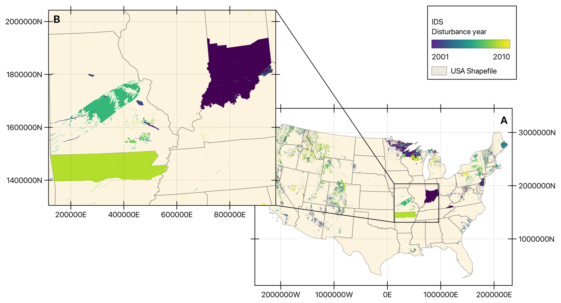
Figure A1Map of IDS with disturbance polygons in the common period 2001–2010 with disturbance events in 2001 in purple to events in 2010 in yellow. Panel (A) shows an overview of the IDS disturbances in the CONUS Region, panel (B) zooms to irregular and large polygons.
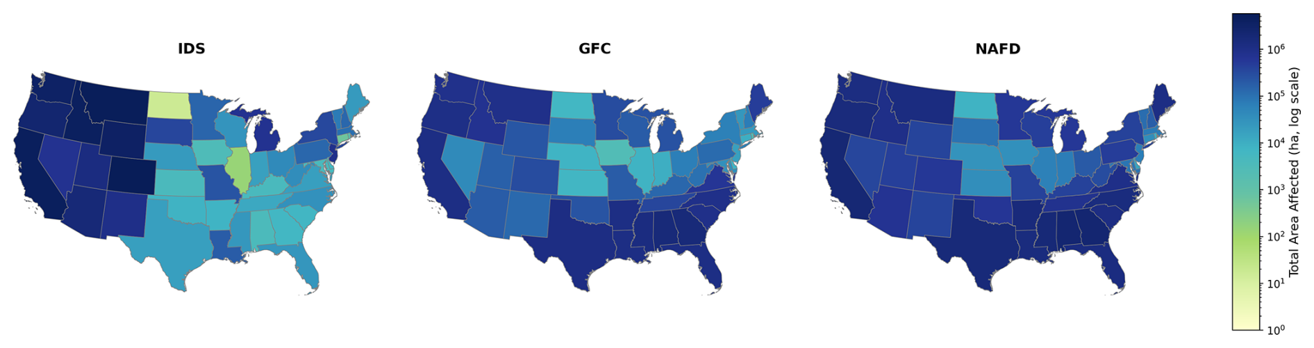
Figure A2Total area affected per state of IDS, GFC and NAFD.

Figure A3Gaussian probability density function of differences in mortality years across CONUS for point-based dataset comparisons. Comparisons are made between small buffers of FIA and ITMN, as well as large buffers of both datasets. Negative values indicate that FIA records mortality earlier than ITMN.
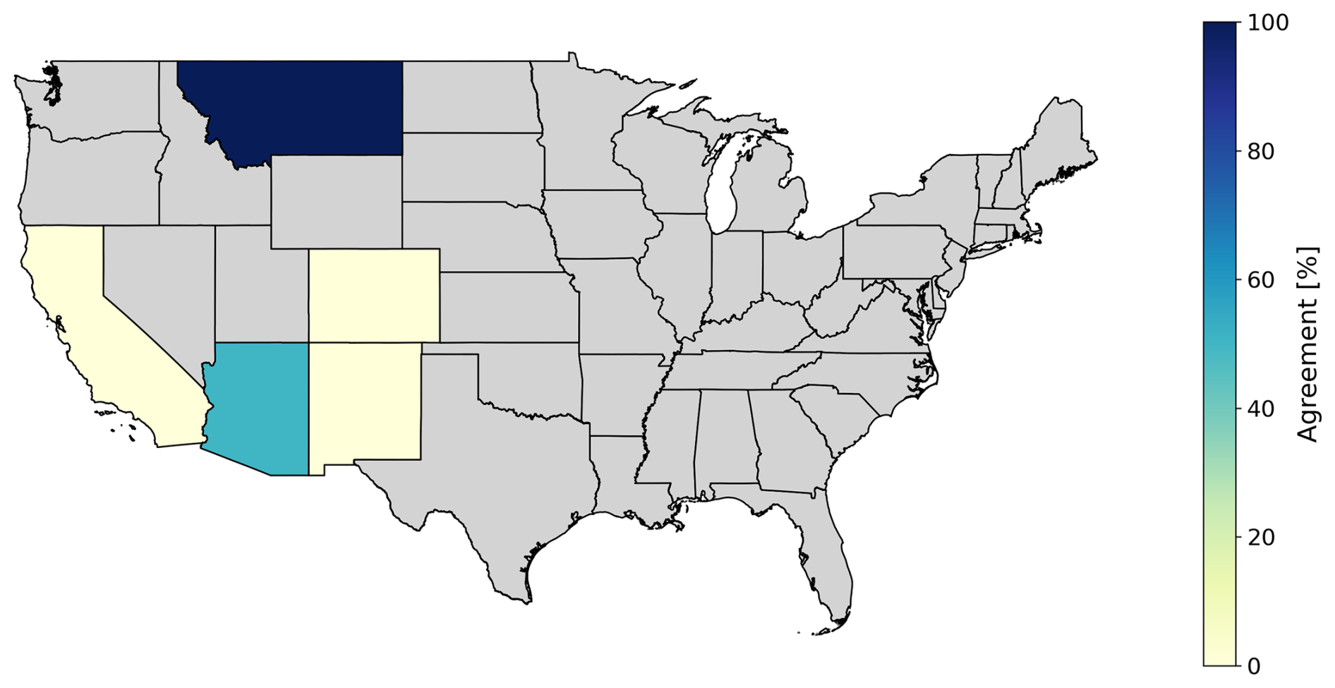
Figure A4DCA agreement between IDS and ITMN by state. Percentages represent the proportion of overlapping disturbance events with matching DCA classifications. Grey states indicate no overlapping events between the two datasets during the study period.
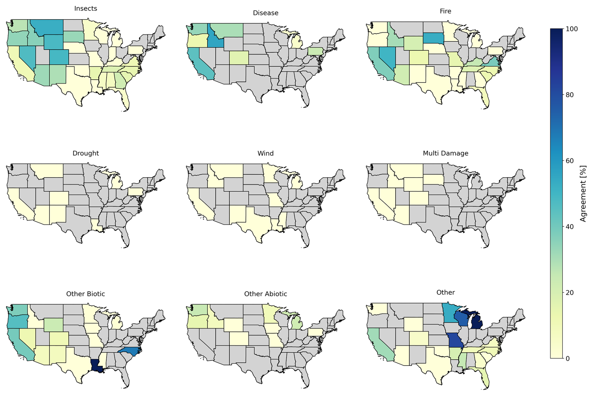
Figure A5DCA agreement between IDS and FIA by state and agent type. Percentages represent the proportion of overlapping disturbance events with matching DCA classifications. Grey states indicate no overlapping events between the two datasets during the study period.
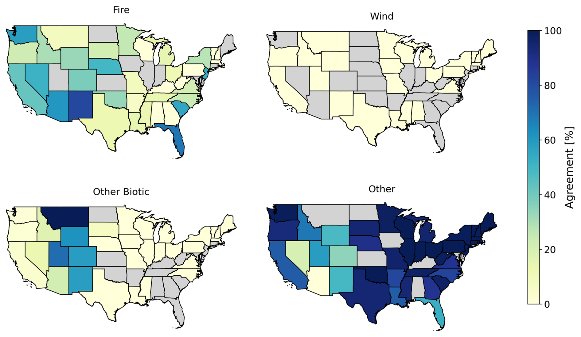
Figure A6DCA agreement between IDS and NAFD by state and agent type. Percentages represent the proportion of overlapping disturbance events with matching DCA classifications. Grey states indicate no overlapping events between the two datasets during the study period.

Figure A7Comparison of mean temporal lag between FIA and IDS across US states, grouped by the difference between public and private forests: (a) private forests and (b) public forests. Negative values (in red) indicate earlier mortality reporting by FIA relative to IDS, while positive values (in blue) indicate later reporting by FIA.
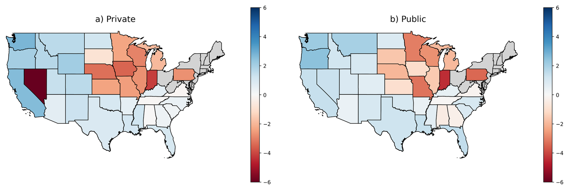
Figure A8Comparison of mean temporal lag between FIA and GFC across US states, grouped by the difference between public and private forests: (a) private forests and (b) public forests. Negative values (in red) indicate earlier mortality reporting by FIA relative to GFC, while positive values (in blue) indicate later reporting by FIA.
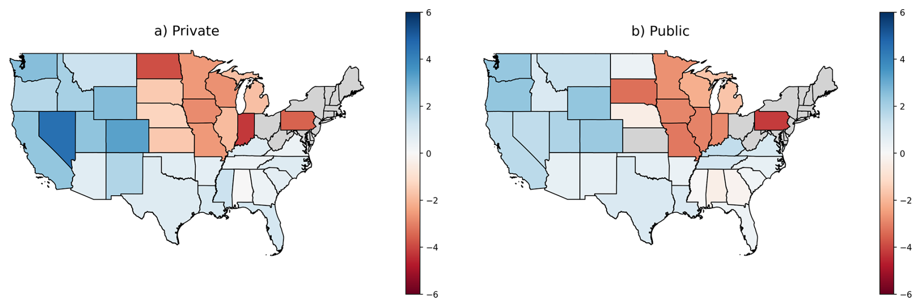
Figure A9Comparison of mean temporal lag between FIA and NAFD across US states, grouped by the difference between public and private forests: (a) private forests and (b) public forests. Negative values (in red) indicate earlier mortality reporting by FIA relative to NAFD, while positive values (in blue) indicate later reporting by FIA.
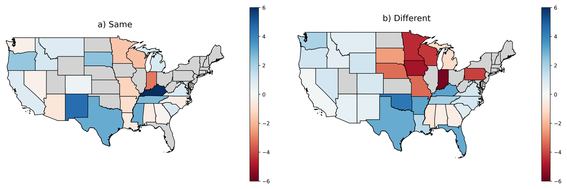
Figure A10Comparison of mean temporal lag between FIA and IDS across US states, grouped by the difference between measurement and mortality year: (a) events with matching years (“Same”) and (b) events with different years (“Different”). Negative values (in red) indicate earlier mortality reporting by FIA relative to IDS, while positive values (in blue) indicate later reporting by FIA.
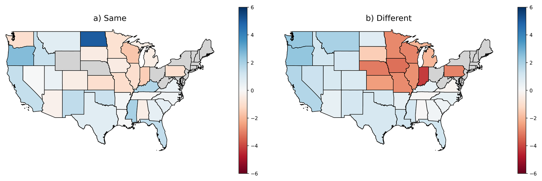
Figure A11Comparison of mean temporal lag between FIA and GFC across US states, grouped by the difference between measurement and mortality year: (a) events with matching years (“Same”) and (b) events with different years (“Different”). Negative values (in red) indicate earlier mortality reporting by FIA relative to GFC, while positive values (in blue) indicate later reporting by FIA.
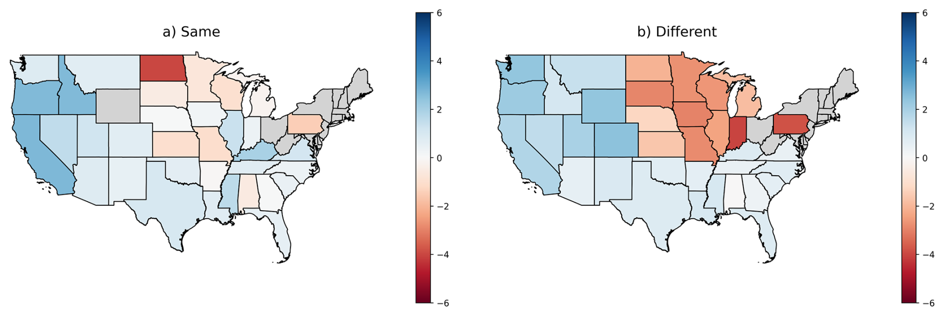
Figure A12Comparison of mean temporal lag between FIA and NAFD across US, grouped by the difference between measurement and mortality year: (a) events with matching years (“Same”) and (b) events with different years (“Different”). Negative values (in red) indicate earlier mortality reporting by FIA relative to NAFD, while positive values (in blue) indicate later reporting by FIA.
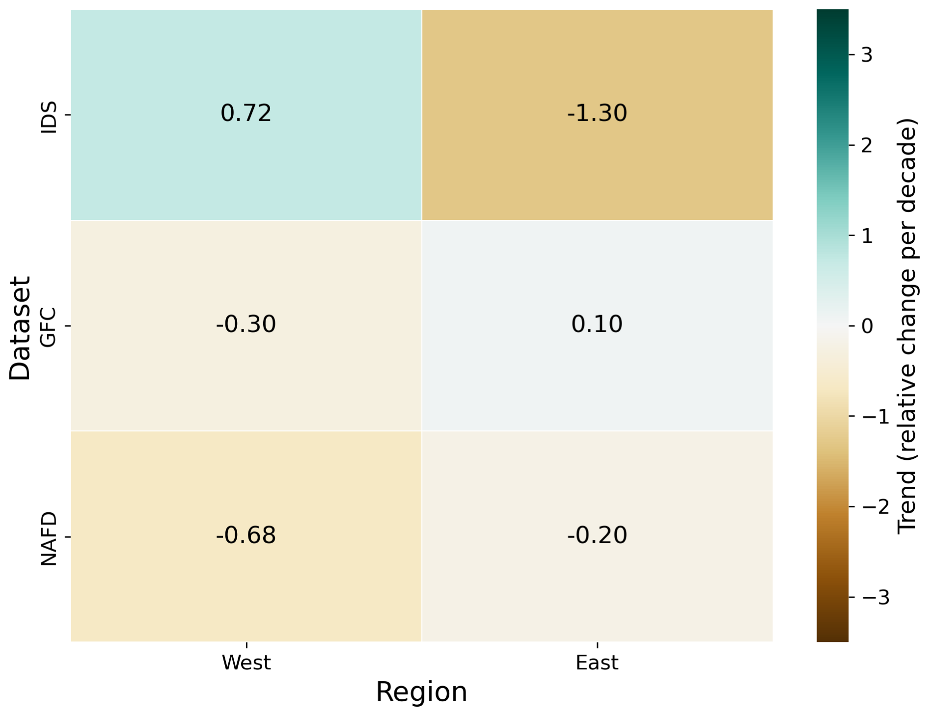
Figure A13Trend of datasets of total area per region. The rows represent the datasets, the columns show the regions (West and East). A positive value indicates an increasing trend compared to the decadal mean.
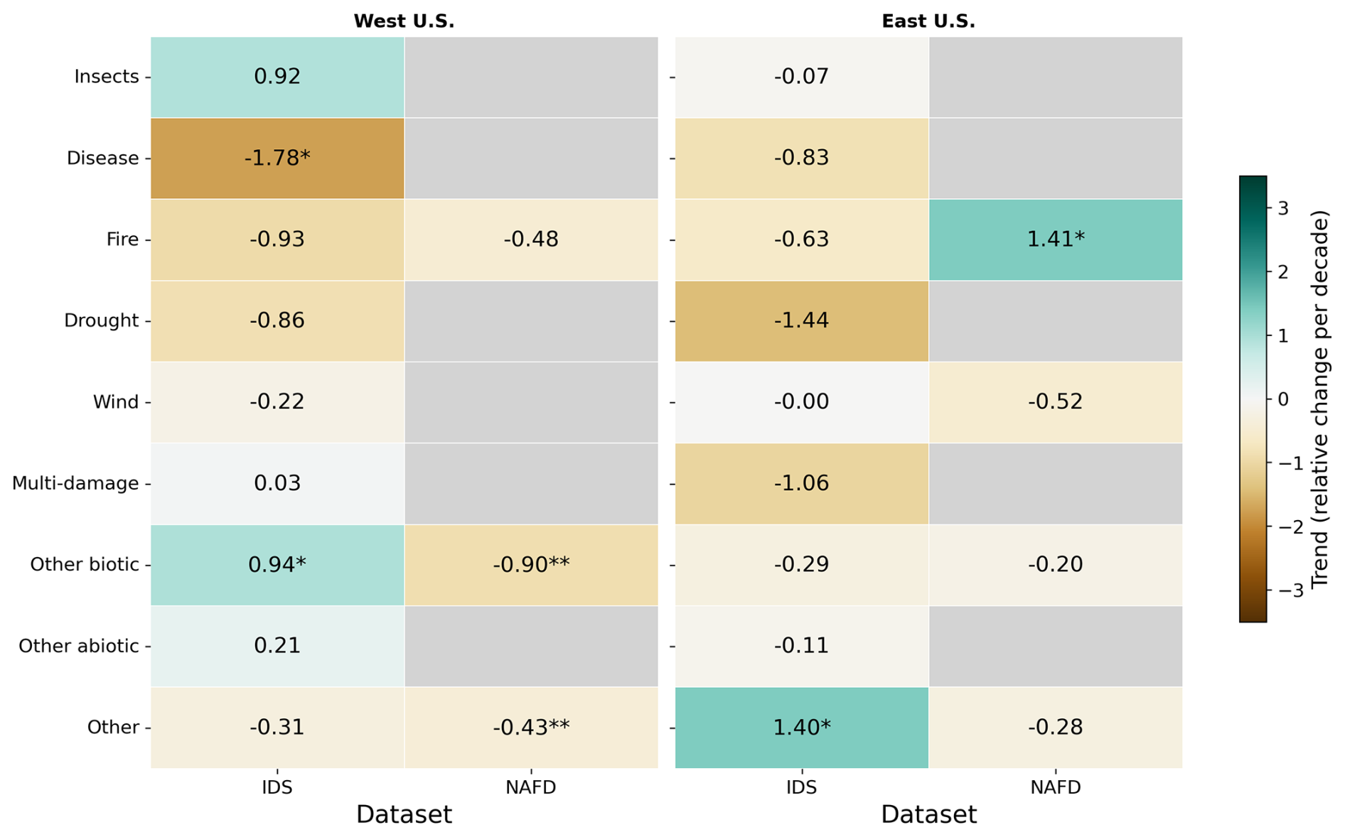
Figure A14Trend of datasets of total area per region with asterisks showing the significance levels (***: p<0.001; **: p<0.01; *: p<0.1). The rows represent the datasets, the columns show the regions (West and East). A positive value indicates an increasing trend compared to the decadal mean. Grey boxes have not enough or no values compute the trend.
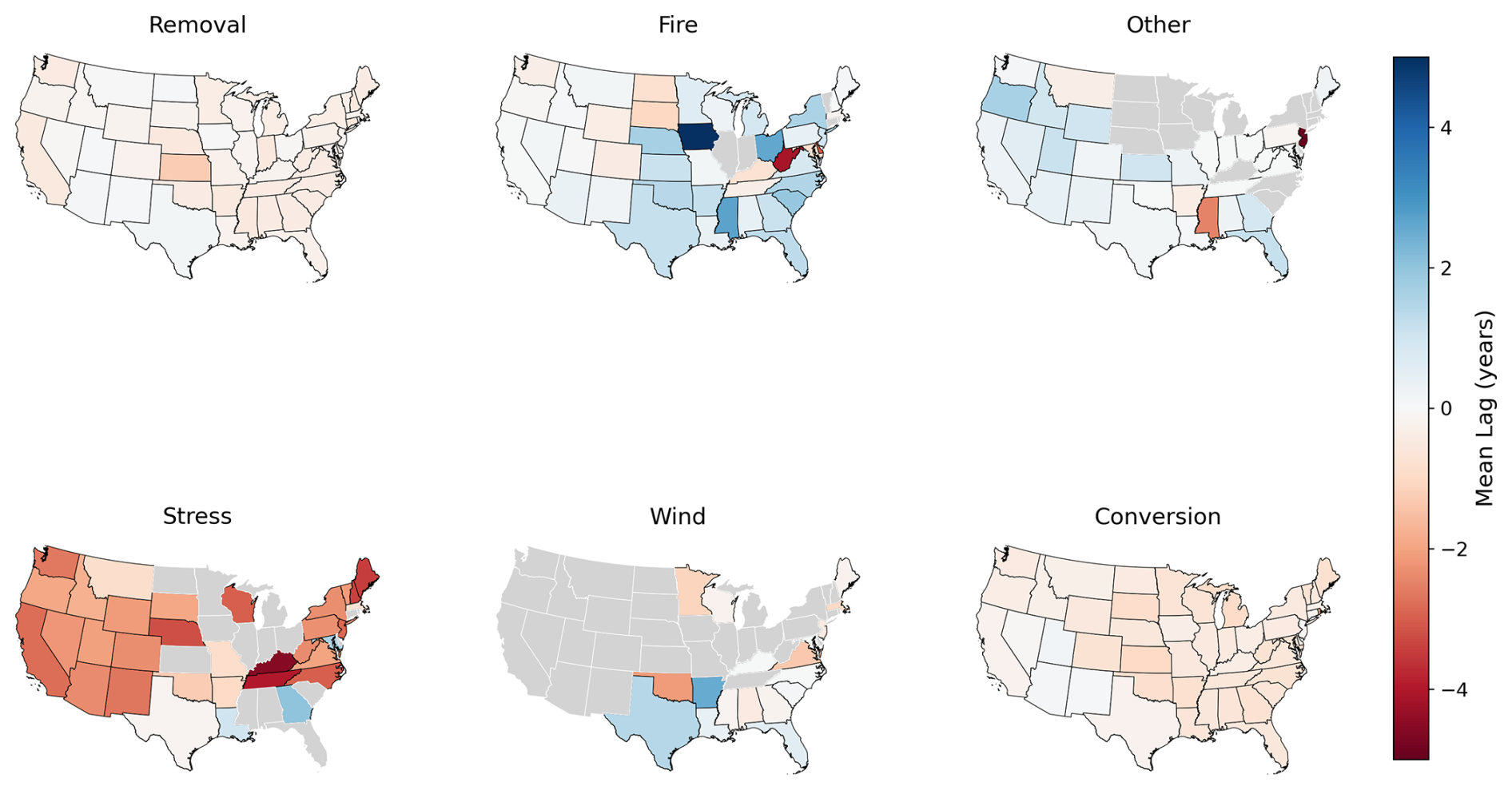
Figure A15Mean lag of overlapping disturbance events in NAFD and GFC per state and original NAFD disturbance agent. Positive values indicate an earlier detection by GFC. Negative values show that NAFD reports earlier.
Table B1Mean and standard deviation values of the differences between pairs of datasets. For the point datasets (FIA, ITMN), two different buffer sizes have been considered to evaluate the role of uncertainty in the reported coordinates. The comparisons are grouped into mixed, spatially explicit, and point-based categories.
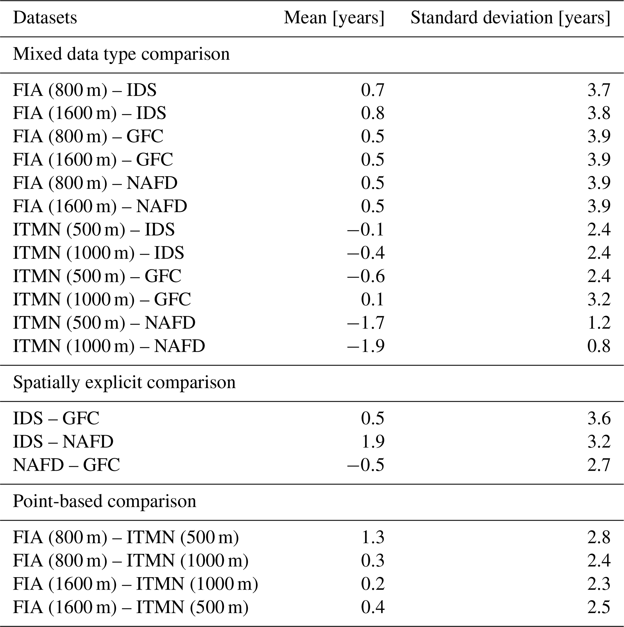
Table B2Mean and standard deviation values of the differences between FIA and IDS, GFC and NAFD, when considering the two groups with different ownership status (public and private).
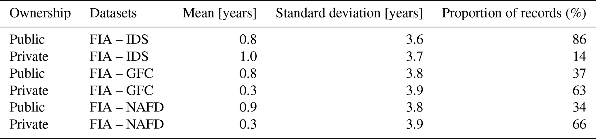
Table B3Mean and standard deviation values of the differences between FIA and IDS, GFC and NAFD, when considering the groups of events with same and different mortality vs. inventory or measurement years.
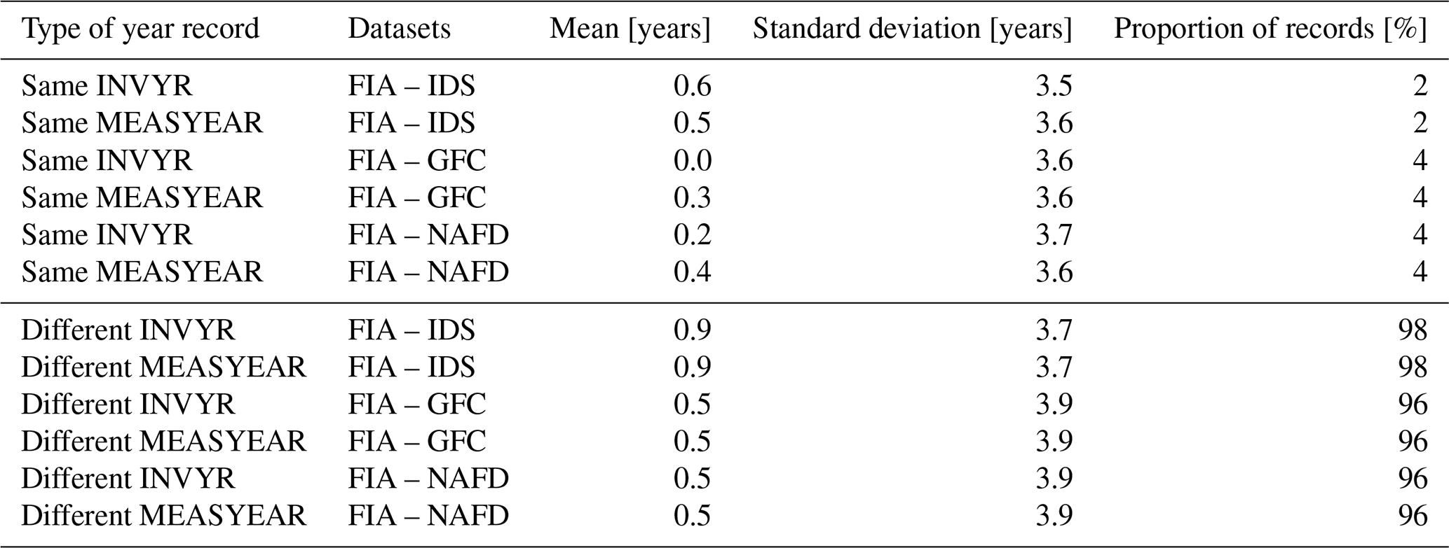
Table B4Agreement matrix showing the absolute counts of overlapping events per disturbance agent between IDS (rows) and NAFD (columns).
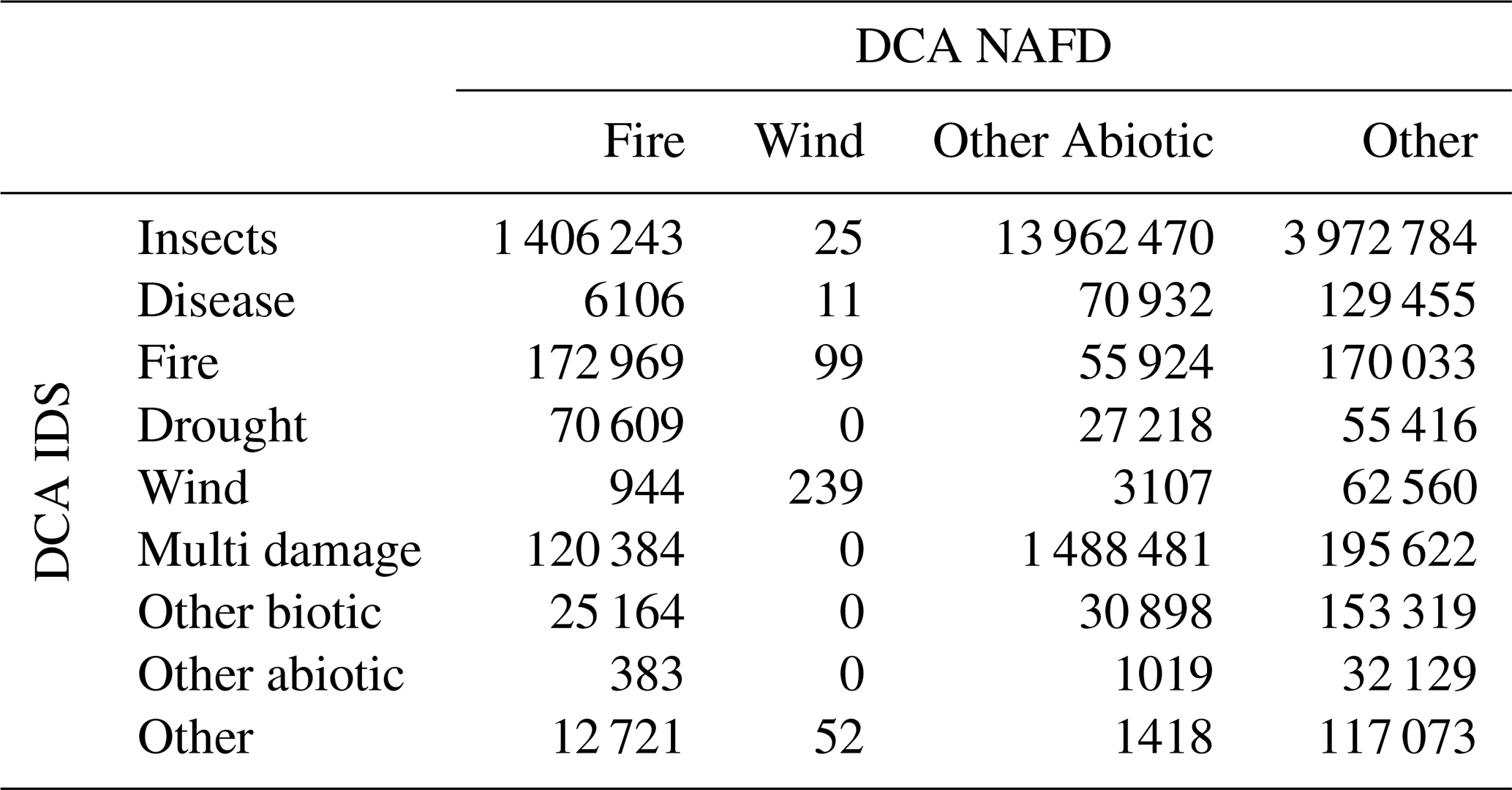
The code to reproduce the analysis and figures is available here: https://github.com/lauraeifler/Eifleretal2026_Disturbance_Data_Comparison (last access: 30 January 2026).
Insect and Disease Survey data by U.S. Department of Agriculture can be downloaded here: https://www.fs.usda.gov/science-technology/data-tools-products/fhp-mapping-reporting/detection-surveys (last access: 28 April 2025); Forest Inventory and Analysis Data by U.S. Department of Agriculture can be downloaded here: https://research.fs.usda.gov/products/dataandtools/tools/fia-datamart (last access: 28 April 2025); Global Tree Mortality Database by the International Tree Mortality Network can be found here: https://www.tree-mortality.net/globaltreemortalitydatabase/ (last access: 28 April 2025); Global forest change data by Global Forest Watch and Global Land Analysis and Discovery can be downloaded here: https://storage.googleapis.com/earthenginepartners-hansen/GFC-2021-v1.9/download.html (last access: 28 April 2025). North American Forest Dynamics Forest Loss Attribution by Schleeweis et al. (2020) can be donwloaded here: https://www.earthdata.nasa.gov/data/catalog/ornl-cloud-nafd-nex-attribution-1799-1 (last access: 28 April 2025).
The supplement related to this article is available online at https://doi.org/10.5194/bg-23-1291-2026-supplement.
AB and LE designed the study. LE conducted the analysis with scientific and technical input by AB and FM. LE wrote the first draft of the paper. All authors contributed to the writing of the MS submitted.
The contact author has declared that none of the authors has any competing interests.
Publisher's note: Copernicus Publications remains neutral with regard to jurisdictional claims made in the text, published maps, institutional affiliations, or any other geographical representation in this paper. The authors bear the ultimate responsibility for providing appropriate place names. Views expressed in the text are those of the authors and do not necessarily reflect the views of the publisher.
Franziska Müller and Ana Bastos acknowledge funding by the European Union (ERC StG, ForExD, grant agreement No. 101039567). This study was supported by the CALIPSO (Carbon Loss In Plants, Soils and Oceans) project, funded through the generosity of Eric and Wendy Schmidt by recommendation of the Schmidt Science program.
This research has been supported by the HORIZON EUROPE European Research Council (grant no. 101039567) and the Schmidt Futures (grant no. G-23-64959).
Supported by the Open Access Publishing Fund
of Leipzig University.
This paper was edited by Andrew Feldman and reviewed by three anonymous referees.
Allen, C. D., Breshears, D. D., and McDowell, N. G.: On underestimation of global vulnerability to tree mortality and forest die-off from hotter drought in the Anthropocene, Ecosphere, 6, art129, https://doi.org/10.1890/ES15-00203.1, 2015. a, b, c, d
Andresini, G., Appice, A., and Malerba, D.: A Deep Semantic Segmentation Approach to Map Forest Tree Dieback in Sentinel-2 Data, IEEE J. Sel. Top. Appl. Earth Obs., 17, 17075–17086, https://doi.org/10.1109/JSTARS.2024.3460981, 2024. a
Banskota, A., Kayastha, N., Falkowski, M. J., Wulder, M. A., Froese, R. E., and White, J. C.: Forest Monitoring Using Landsat Time Series Data: A Review, Can. J. Remote Sens., 40, 362–384, https://doi.org/10.1080/07038992.2014.987376, 2014. a
Bárta, V., Lukeš, P., and Homolová, L.: Early detection of bark beetle infestation in Norway spruce forests of Central Europe using Sentinel-2, International Journal of Applied Earth Observation and Geoinformation, 100, 102335, https://doi.org/10.1016/j.jag.2021.102335, 2021. a
Bastos, A., Orth, R., Reichstein, M., Ciais, P., Viovy, N., Zaehle, S., Anthoni, P., Arneth, A., Gentine, P., Joetzjer, E., Lienert, S., Loughran, T., McGuire, P. C., O, S., Pongratz, J., and Sitch, S.: Vulnerability of European ecosystems to two compound dry and hot summers in 2018 and 2019, Earth Syst. Dynam., 12, 1015–1035, https://doi.org/10.5194/esd-12-1015-2021, 2021. a
Bastos, A., Sippel, S., Frank, D., Mahecha, M. D., Zaehle, S., Zscheischler, J., and Reichstein, M.: A joint framework for studying compound ecoclimatic events, Nat. Rev. Earth Environ., 4, 333–350, https://doi.org/10.1038/s43017-023-00410-3, 2023. a
Bentz, B. J., Régnière, J., Fettig, C. J., Hansen, E. M., Hayes, J. L., Hicke, J. A., Kelsey, R. G., Negrón, J. F., and Seybold, S. J.: Climate Change and Bark Beetles of the Western United States and Canada: Direct and Indirect Effects, BioScience, 60, 602–613, https://doi.org/10.1525/bio.2010.60.8.6, 2010. a
Bonan, G. B.: Forests and Climate Change: Forcings, Feedbacks, and the Climate Benefits of Forests, Science, 320, 1444–1449, https://doi.org/10.1126/science.1155121, 2008. a
Bowman, D. M. J. S., Balch, J. K., Artaxo, P., Bond, W. J., Carlson, J. M., Cochrane, M. A., D'Antonio, C. M., DeFries, R. S., Doyle, J. C., Harrison, S. P., Johnston, F. H., Keeley, J. E., Krawchuk, M. A., Kull, C. A., Marston, J. B., Moritz, M. A., Prentice, I. C., Roos, C. I., Scott, A. C., Swetnam, T. W., van der Werf, G. R., and Pyne, S. J.: Fire in the Earth System, Science, 324, 481–484, https://doi.org/10.1126/science.1163886, 2009. a
Burrill, E. A., DiTommaso, A. M., Turner, J. A., Pugh, S. A., Menlove James, C. G., Perry, C. J., and Conkling, B. L.: The Forest Inventory and Analysis Database: Database Description and User Guide for Phase 2 (Version 9.0.1), U.S. Department of Agriculture, Forest Service, 29, 1026, https://research.fs.usda.gov/understory/forest-inventory-and-analysis-database-user-guide-nfi (last access: 6 February 2026), 2021. a, b, c
Burton, P. J., Jentsch, A., and Walker, L. R.: The Ecology of Disturbance Interactions, BioScience, 70, 854–870, https://doi.org/10.1093/biosci/biaa088, 2020. a
Chuvieco, E., Lizundia-Loiola, J., Pettinari, M. L., Ramo, R., Padilla, M., Tansey, K., Mouillot, F., Laurent, P., Storm, T., Heil, A., and Plummer, S.: Generation and analysis of a new global burned area product based on MODIS 250 m reflectance bands and thermal anomalies, Earth Syst. Sci. Data, 10, 2015–2031, https://doi.org/10.5194/essd-10-2015-2018, 2018. a
Chuvieco, E., Roteta, E., Sali, M., Stroppiana, D., Boettcher, M., Kirches, G., Storm, T., Khairoun, A., Pettinari, M. L., Franquesa, M., and Albergel, C.: Building a small fire database for Sub-Saharan Africa from Sentinel-2 high-resolution images, Sci. Total Environ., 845, 157139, https://doi.org/10.1016/j.scitotenv.2022.157139, 2022. a
Clark, J. S., Iverson, L., Woodall, C. W., Allen, C. D., Bell, D. M., Bragg, D. C., D'Amato, A. W., Davis, F. W., Hersh, M. H., Ibanez, I., Jackson, S. T., Matthews, S., Pederson, N., Peters, M., Schwartz, M. W., Waring, K. M., and Zimmermann, N. E.: The impacts of increasing drought on forest dynamics, structure, and biodiversity in the United States, Global Change Biol., 22, 2329–2352, https://doi.org/10.1111/gcb.13160, 2016. a
Cohen, W., Healey, S., Yang, Z., Stehman, S., Brewer, C., Brooks, E., Gorelick, N., Huang, C., Hughes, M., Kennedy, R., Loveland, T., Moisen, G., Schroeder, T., Vogelmann, J., Woodcock, C., Yang, L., and Zhu, Z.: How Similar Are Forest Disturbance Maps Derived from Different Landsat Time Series Algorithms?, Forests, 8, 98, https://doi.org/10.3390/f8040098, 2017. a
Cohen, W. B., Yang, Z., Stehman, S. V., Schroeder, T. A., Bell, D. M., Masek, J. G., Huang, C., and Meigs, G. W.: Forest disturbance across the conterminous United States from 1985–2012: The emerging dominance of forest decline, Forest Ecol. Manage., 360, 242–252, https://doi.org/10.1016/j.foreco.2015.10.042, 2016. a, b, c, d
Coleman, T. W., Graves, A. D., Heath, Z., Flowers, R. W., Hanavan, R. P., Cluck, D. R., and Ryerson, D.: Accuracy of aerial detection surveys for mapping insect and disease disturbances in the United States, Forest Ecol. Manage., 430, 321–336, https://doi.org/10.1016/j.foreco.2018.08.020, 2018. a, b, c, d, e
Coops, N. C., Tompalski, P., Goodbody, T. R. H., Achim, A., and Mulverhill, C.: Framework for near real-time forest inventory using multi source remote sensing data, Forestry, 96, 1–19, 2023. a
Curtis, P. G., Slay, C. M., Harris, N. L., Tyukavina, A., and Hansen, M. C.: Classifying drivers of global forest loss, Science, 361, 1108–1111, https://doi.org/10.1126/science.aau3445, 2018. a, b
DeFries, R. S., Rudel, T., Uriarte, M., and Hansen, M.: Deforestation driven by urban population growth and agricultural trade in the twenty-first century, Nat. Geosci., 3, 178–181, 2010. a
European Commission: Directorate-General for Environment, Atzberger, C., Defourny, P., Aragão, L., Hammarström, L., and Immitzer, M.: Monitoring of forests through remote sensing – Final report, Publications Office, https://doi.org/10.2779/175242, 2020. a
FAO: Global Forest Resources Assessment 2010 (FRA2010), Tech. rep., Food and Agriculture Organization of the United Nations, Rome, 2010. a
FAO: Global Forest Resources Assessment 2015 (FRA2015), Tech. rep., Food and Agriculture Organization of the United Nations, Rome, 2015. a
FAO: Global Forest Resources Assessment 2020 (FRA2020), Tech. rep., Food and Agriculture Organization of the United Nations, Rome, https://doi.org/10.4060/ca9825en, 2020. a
Fettig, C. J., Egan, J. M., Delb, H., Hilszczan´ski, J., Kautz, M., Munson, A. S., Nowak, J. T., and Negró, J. F.: Management tactics to reduce bark beetle impacts in North America and Europe under altered forest and climatic conditions, in: Bark Beetle Management, Ecology, and Climate Change, edited by: Gandhi, K. J. K. and Hofstetter, R. W., 345–394, Academic Press, ISBN 978-0-12-822145-7, https://doi.org/10.1016/B978-0-12-822145-7.00006-4, 2022. a
Forest Service U.S. Department of Agriculture: FIA DataMart, https://research.fs.usda.gov/products/dataandtools/fia-datamart (last access: 30 January 2026), 2023. a, b
Forest Service U.S. Department of Agriculture: Detection Surveys, https://www.fs.usda.gov/science-technology/data-tools-products/fhp-mapping-reporting/detection-surveys (last access: 12 March 2024), 2024. a, b, c
Forzieri, G., Pecchi, M., Girardello, M., Mauri, A., Klaus, M., Nikolov, C., Rüetschi, M., Gardiner, B., Tomaštík, J., Small, D., Nistor, C., Jonikavicius, D., Spinoni, J., Feyen, L., Giannetti, F., Comino, R., Wolynski, A., Pirotti, F., Maistrelli, F., Savulescu, I., Wurpillot-Lucas, S., Karlsson, S., Zieba-Kulawik, K., Strejczek-Jazwinska, P., Mokroš, M., Franz, S., Krejci, L., Haidu, I., Nilsson, M., Wezyk, P., Catani, F., Chen, Y.-Y., Luyssaert, S., Chirici, G., Cescatti, A., and Beck, P. S. A.: A spatially explicit database of wind disturbances in European forests over the period 2000–2018, Earth Syst. Sci. Data, 12, 257–276, https://doi.org/10.5194/essd-12-257-2020, 2020. a
Forzieri, G., Girardello, M., Ceccherini, G., Spinoni, J., Feyen, L., Hartmann, H., Beck, P. S. A., Camps-Valls, G., Chirici, G., Mauri, A., and Cescatti, A.: Emergent vulnerability to climate-driven disturbances in European forests, Nat. Commun., 12, 1081, https://doi.org/10.1038/s41467-021-21399-7, 2021. a
Forzieri, G., Dutrieux, L. P., Elia, A., Eckhardt, B., Caudullo, G., Álvarez Taboada, F., Andriolo, A., Bălăcenoiu, F., Bastos, A., Buzatu, A., Castedo Dorado, F., Dobrovolný, L., Duduman, M.-L., Fernandez-Carrillo, A., Cescatti, A., A Beck, P. S., Giovanni Forzieri, C., and Commission, E.: The Database of European Forest Insect and Disease Disturbances: DEFID2, Glob. Change Biol., 29, 6040–6065, https://doi.org/10.1111/gcb.16912, 2023. a, b, c, d
Gao, Y., Skutsch, M., Paneque-Gálvez, J., and Ghilhardi, A.: Remote sensing of forest degradation: a review, Environ. Res. Lett., 15, 103001, https://doi.org/10.1088/1748-9326/abaad7, 2020. a
Gibson, R., Danaher, T., Hehir, W., and Collins, L.: A remote sensing approach to mapping fire severity in south-eastern Australia using sentinel 2 and random forest, Remote Sens. Environ., 240, 111702, https://doi.org/10.1016/j.rse.2020.111702, 2020. a
Hammond, W. M., H., Williams, A. P., Abatzoglou, J. T., Adams, H. D., Klein, T., López Rodríguez, R., Sáenz-Romero, C., Hartmann, H., Breshears, D. D., and Allen, C. D.: Global field observations of tree die-off reveal hotter-drought fingerprint for Earth's forests, Nat. Commun., 13, 1761, https://doi.org/10.1038/s41467-022-29289-2, 2022. a, b, c, d, e, f, g, h, i
Hansen, M., Potapov, P. V., Moore, R., Hancher, M., Turubanova, S., Tyukavina, A., Thau, D., Stehman, S., Goetz, S., Loveland, T., Kommareddy, A., Egorov, A., Chini, L., Justice, C., and Townshed, J.: Global Forest Change 2000–2024 Data Download, https://storage.googleapis.com/earthenginepartners-hansen/GFC-2024-v1.12/download.html (last access: 28 April 2025), 2024. a, b
Hansen, M. C., Potapov, P. V., Moore, R., Hancher, M., Turubanova, S. A., Tyukavina, A., Thau, D., Stehman, S. V., Goetz, S. J., Loveland, T. R., Kommareddy, A., Egorov, A., Chini, L., Justice, C. O., and Townshend, J. R.: High-resolution global maps of 21st-century forest cover change, Science, 342, 850–853, https://doi.org/10.1126/SCIENCE.1244693, 2013. a, b, c, d, e, f, g, h, i, j
Harris, N. L., Hagen, S. C., Saatchi, S. S., Pearson, T. R. H., Woodall, C. W., Domke, G. M., Braswell, B. H., Walters, B. F., Brown, S., Salas, W., Fore, A., and Yu, Y.: Attribution of net carbon change by disturbance type across forest lands of the conterminous United States, Carbon Balance and Management, 11, 24, https://doi.org/10.1186/s13021-016-0066-5, 2016. a
Hartmann, H., Bastos, A., Das, A. J., Esquivel-Muelbert, A., Hammond, W. M., Martínez-Vilalta, J., McDowell, N. G., Powers, J. S., Pugh, T. A., and Ruthrof, K. X.: Climate change risks to global forest health: emergence of unexpected events of elevated tree mortality worldwide, Annu. Rev. Plant Biol., 73, 673–702, 2022. a
Hawryło, P., Bednarz, B., Wężyk, P., and Szostak, M.: Estimating defoliation of Scots pine stands using machine learning methods and vegetation indices of Sentinel-2, European Journal of Remote Sensing, 51, 194–204, https://doi.org/10.1080/22797254.2017.1417745, 2018. a
Hicke, J. A., Allen, C. D., Desai, A. R., Dietze, M. C., Hall, R. J., Hogg, E. H., Kashian, D. M., Moore, D., Raffa, K. F., Sturrock, R. N., and Vogelmann, J.: Effects of biotic disturbances on forest carbon cycling in the United States and Canada, Global Change Biol., 18, 7–34, 2012. a, b
Hicke, J. A., Xu, B., Meddens, A. J. H., and Egan, J. M.: Characterizing recent bark beetle-caused tree mortality in the western United States from aerial surveys, Forest Ecol. Manage., 475, 118402, https://doi.org/10.1016/j.foreco.2020.118402, 2020. a, b
Hou, J., Huang, C., Chen, W., and Zhang, Y.: Improving Snow Estimates Through Assimilation of MODIS Fractional Snow Cover Data Using Machine Learning Algorithms and the Common Land Model, Water Resour. Res., 57, https://doi.org/10.1029/2020WR029010, 2021. a
International tree mortality network: Global Tree Mortality Database, https://www.tree-mortality.net/globaltreemortalitydatabase/ (last access: 28 April 2022), 2022. a, b
Kautz, M., Meddens, A. J. H., Hall, R. J., and Arneth, A.: Biotic disturbances in Northern Hemisphere forests-a synthesis of recent data, uncertainties and implications for forest monitoring and modelling, Global Ecology and Biogeography, 26, 533–552, https://doi.org/10.1111/geb.12558, 2017. a, b, c, d
Kendall, M. and Gibbons, J. D.: Rank correlation measures, Charles Griffin book series, Oxford University Press, London, 202, 0195208374, 1990. a
Knott, J. A., Liknes, G. C., Giebink, C. L., Oh, S., Domke, G. M., McRoberts, R. E., Quirino, V. F., and Walters, B. F.: Effects of outliers on remote sensing-assisted forest biomass estimation: A case study from the United States national forest inventory, Meth. Ecol. Evol., 14, 1587–1602, 2023. a
Kurz, W. A., Dymond, C. C., Stinson, G., Rampley, G. J., Neilson, E. T., Carroll, A. L., Ebata, T., and Safranyik, L.: Mountain pine beetle and forest carbon feedback to climate change, Nature, 452, 987–990, https://doi.org/10.1038/nature06777, 2008. a
Lindner, M., Maroschek, M., Netherer, S., Kremer, A., Barbati, A., Garcia-Gonzalo, J., Seidl, R., Delzon, S., Corona, P., Kolström, M., Lexer, M. J., and Marchetti, M.: Climate change impacts, adaptive capacity, and vulnerability of European forest ecosystems, Forest Ecol. Manage., 259, 698–709, https://doi.org/10.1016/j.foreco.2009.09.023, 2010. a
Mann, H. B.: Nonparametric tests against trend, Econometrica: Journal of the Econometric Society, 13, 245–259, 1945. a
Masek, J. G., Goward, S. N., Kennedy, R. E., Cohen, W. B., Moisen, G. G., Schleeweis, K., and Huang, C.: United States Forest Disturbance Trends Observed Using Landsat Time Series, Ecosystems, 16, 1087–1104, https://doi.org/10.1007/s10021-013-9669-9, 2013. a, b, c
Masson-Delmotte, V., Zhai, P., Pirani, A., Connors, S. L., Péan, C., Berger, S., Caud, N., Chen, Y., Goldfarb, L., and Gomis, M.: Climate change 2021: the physical science basis, Contribution of working group I to the sixth assessment report of the intergovernmental panel on climate change, Geneva, Switzerland, 2, https://doi.org/10.1017/9781009157896, 2021. a
McDowell, N. G., Coops, N. C., Beck, P. S., Chambers, J. Q., Gangodagamage, C., Hicke, J. A., Huang, C.-y., Kennedy, R., Krofcheck, D. J., Litvak, M., Meddens, A. J., Muss, J., Negrón-Juarez, R., Peng, C., Schwantes, A. M., Swenson, J. J., Vernon, L. J., Williams, A. P., Xu, C., Zhao, M., Running, S. W., and Allen, C. D.: Global satellite monitoring of climate-induced vegetation disturbances, Trends in Plant Science, 20, 114–123, https://doi.org/10.1016/j.tplants.2014.10.008, 2015. a, b, c, d, e, f
McDowell, N. G., Allen, C. D., Anderson-Teixeira, K., Aukema, B. H., Bond-Lamberty, B., Chini, L., Clark, J. S., Dietze, M., Grossiord, C., Hanbury-Brown, A., Hurtt, G. C., Jackson, R. B., Johnson, D. J., Kueppers, L., Lichstein, J. W., Ogle, K., Poulter, B., Pugh, T. A. M., Seidl, R., Turner, M. G., Uriarte, M., Walker, A. P., and Xu, C.: Pervasive shifts in forest dynamics in a changing world, Science, 368, eaaz9463, https://doi.org/10.1126/science.aaz9463, 2020. a
Meddens, A. J. H., Hicke, J. A., and Ferguson, C. A.: Spatiotemporal patterns of observed bark beetle-caused tree mortality in British Columbia and the western United States, Ecol. Appl., 22, 1876–1891, 2012. a, b, c, d
Meigs, G. W., Morrissey, R. C., Bače, R., Chaskovskyy, O., Čada, V., Després, T., Donato, D. C., Janda, P., Lábusová, J., Seedre, M., Mikoláš, M., Nagel, T. A., Schurman, J. S., Synek, M., Teodosiu, M., Trotsiuk, V., Vítková, L., and Svoboda, M.: More ways than one: Mixed-severity disturbance regimes foster structural complexity via multiple developmental pathways, Forest Ecol. Manage., 406, 410–426, https://doi.org/10.1016/j.foreco.2017.07.051, 2017. a
Müller, F., Eifler, L., Cremer, F., Beck, P., Camps-Valls, G., and Bastos, A.: Hybrid forest disturbance classification using Sentinel-1 and inventory data: a case-study for Southeastern USA, EGUsphere [preprint], https://doi.org/10.5194/egusphere-2025-4880, 2025. a, b
Otón, G., Ramo, R., Lizundia-Loiola, J., and Chuvieco, E.: Global Detection of Long-Term (1982–2017) Burned Area with AVHRR-LTDR Data, Remote Sens., 11, 2079, https://doi.org/10.3390/rs11182079, 2019. a
Patacca, M., Schelhaas, M.-J., Zudin, S., and Lindner, M.: Database on Forest Disturbances in Europe (DFDE)-Technical report History, State of the Art, and Future Perspectives, Project I-Maestro (ERA-NET Cofund ForestValue), 2021. a
Patacca, M., Lindner, M., Lucas-Borja, M. E., Cordonnier, T., Fidej, G., Gardiner, B., Hauf, Y., Jasinevičius, G., Labonne, S., Linkevičius, E., Mahnken, M., Milanovic, S., Nabuurs, G.-J., Nagel, T. A., Nikinmaa, L., Panyatov, M., Bercak, R., Seidl, R., Ostrogović Sever, M. Z., Socha, J., Thom, D., Vuletic, D., Zudin, S., and Schelhaas, M.-J.: Significant increase in natural disturbance impacts on European forests since 1950, Global Change Biol., 29, 1359–1376, https://doi.org/10.1111/gcb.16531, 2023. a, b, c
Potapov, P., Hansen, M. C., Stehman, S. V., Loveland, T. R., and Pittman, K.: Combining MODIS and Landsat imagery to estimate and map boreal forest cover loss, Remote Sens. Environ., 112, 3708–3719, https://doi.org/10.1016/j.rse.2008.05.006, 2008. a
Prasad, A., Iverson, L., and Liaw, A.: Newer classification and regression tree techniques: bagging and random forests for ecological prediction, Ecosystems, 9, 181–199, 2006. a, b
Schleeweis, K. G., Moisen, G. G., Schroeder, T. A., Toney, C., Freeman, E. A., Goward, S. N., Huang, C., and Dungan, J. L.: US National Maps Attributing Forest Change: 1986–2010, Forests, 11, 653, https://doi.org/10.3390/f11060653, 2020. a, b, c, d, e, f, g, h, i, j
Schroeder, T. A., Healey, S. P., Moisen, G. G., Frescino, T. S., Cohen, W. B., Huang, C., Kennedy, R. E., and Yang, Z.: Improving estimates of forest disturbance by combining observations from Landsat time series with U.S. Forest Service Forest Inventory and Analysis data, Remote Sens. Environ., 154, 61–73, https://doi.org/10.1016/j.rse.2014.08.005, 2014. a, b, c, d, e
Seidl, R. and Turner, M. G.: Post-disturbance reorganization of forest ecosystems in a changing world, P. Natl. Acad. Sci. USA, 119, e2202190119, https://doi.org/10.1073/pnas.2202190119, 2022. a
Seidl, R., Schelhaas, M.-J., and Lexer, M. J.: Unraveling the drivers of intensifying forest disturbance regimes in Europe, Global Change Biol., 17, 2842–2852, https://doi.org/10.1111/j.1365-2486.2011.02452.x, 2011. a, b
Seidl, R., Thom, D., Kautz, M., Martin-Benito, D., Peltoniemi, M., Vacchiano, G., Wild, J., Ascoli, D., Petr, M., Honkaniemi, J., Lexer, M. J., Trotsiuk, V., Mairota, P., Svoboda, M., Fabrika, M., Nagel, T. A., and Reyer, C. P.: Forest disturbances under climate change, Nat. Clim. Change, 7, 395–402, https://doi.org/10.1038/NCLIMATE3303, 2017. a, b, c
Sen, P. K.: Estimates of the regression coefficient based on Kendall's tau, J. Am. Stat. A., 63, 1397–1412, 1968. a
Senf, C. and Seidl, R.: Persistent impacts of the 2018 drought on forest disturbance regimes in Europe, Biogeosciences, 18, 5223–5230, https://doi.org/10.5194/bg-18-5223-2021, 2021a. a
Senf, C. and Seidl, R.: Storm and fire disturbances in Europe: Distribution and trends, Global Change Biol., 27, 3605–3619, https://doi.org/10.1111/gcb.15679, 2021b. a, b, c
Senf, C., Pflugmacher, D., Wulder, M. A., and Hostert, P.: Characterizing spectral–temporal patterns of defoliator and bark beetle disturbances using Landsat time series, Remote Sens. Environ., 170, 166–177, https://doi.org/10.1016/j.rse.2015.09.019, 2015. a
Senf, C., Seidl, R., and Hostert, P.: Remote sensing of forest insect disturbances: Current state and future directions, International Journal of Applied Earth Observation and Geoinformation, 60, 49–60, 2017. a
Senf, C., Buras, A., Zang, C. S., Rammig, A., and Seidl, R.: Excess forest mortality is consistently linked to drought across Europe, Nat. Commun., 11, 6200, https://doi.org/10.1038/s41467-020-19924-1, 2020. a, b, c
Sommerfeld, A., Senf, C., Buma, B., D'Amato, A. W., Després, T., and Díaz-Hormazábal, I.: Patterns and drivers of recent disturbances across the temperate forest biome, Nat. Commun., 9, 4355, https://doi.org/10.1038/s41467-018-06788-9, 2018. a
Thom, D. and Seidl, R.: Natural disturbance impacts on ecosystem services and biodiversity in temperate and boreal forests, Biol. Rev., 91, 760–781, https://doi.org/10.1111/brv.12193, 2016. a, b, c
Thompson, M.: Analysis of conifer mortality in Colorado using forest inventory and analysis's annual forest inventory, Western Journal of Applied Forestry, 24, 193–197, 2009. a
Tinkham, W. T., Mahoney, P. R., Hudak, A. T., Domke, G. M., Falkowski, M. J., Woodall, C. W., and Smith, A. M.: Applications of the United States forest inventory and analysis dataset: A review and future directions, Can. J. Forest Res., 48, 1251–1268, https://doi.org/10.1139/cjfr-2018-0196, 2018. a, b
Turner, M. G.: Disturbance and landscape dynamics in a changing world, Ecology, 91, 2833–2849, https://doi.org/10.1890/10-0097.1, 2010. a, b, c
U.S. Geological Survey: USGS 1 arc-second DEM, https://www.usgs.gov/the-national-map-data-delivery/gis-data-download (last access: 30 April 2025), 2025. a
White, P. S. and Pickett, S. T. A.: Chapter 1 – Natural Disturbance and Patch Dynamics: An Introduction, in: The Ecology of Natural Disturbance and Patch Dynamics, edited by: Pickett, S. T. A. and White, P. S., 3–13, Academic Press, San Diego, ISBN 978-0-12-554520-4, https://doi.org/10.1016/B978-0-12-554520-4.50006-X, 1985. a