Spatial variability of greenhouse gas concentrations and fluxes in shallow coastal bays of the western Baltic Sea

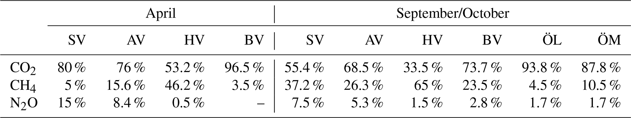
Coastal ecosystems play a crucial role in greenhouse gas (GHG) dynamics but are less studied than open oceans or terrestrial systems. This study measured concentrations of carbon dioxide (CO₂), methane (CH₄), and nitrous oxide (N₂O) in six shallow bays of the wider Stockholm Archipelago during spring (April) and autumn (September–October) 2024 using cavity ring-down spectroscopy combined with a water equilibration system. We explored how GHG levels relate to bay physical characteristics (i.e. topographic openness, sediment properties vegetation cover) and seawater properties (temperature, salinity, dissolved-oxygen saturation, chlorophyll-a, organic carbon, and nutrient concentrations), revealing significant seasonal variation of concentrations. Surface water pCO₂ ranged from 225–1372 ppm, CH₄ from 3.6–580 nmol L⁻¹, and N₂O from 8–20.8 nmol L⁻¹ with pCO₂ and CH₄ higher in autumn and N₂O higher in spring. CH₄ concentrations below 250 nmol L⁻¹ were negatively correlated with N₂O, while higher CH₄ levels showed a positive correlation, suggesting differences in the dominant sedimentary microbial pathways. Most bays acted as net GHG sinks in April and sources in September, with only one bay showing net source behaviour in both seasons. One bay that is subject to substantial human impacts (e.g. dredging, high nutrient loading, reduced vegetation cover) showed CO₂-equivalent CH₄ emissions that surpassed CO₂ uptake in this particular bay. CO₂-equivalent fluxes ranged from −195.2 to 793.6 mg CO₂ eq. m⁻² d⁻¹ (median: 131.5 mg CO₂ eq. m⁻² d⁻¹). This study is distinctive in simultaneously measuring all three major GHGs across multiple bays in relation to diverse environmental controls, offering a uniquely integrated understanding of coastal GHG dynamics. These findings highlight the variability and complexity of coastal ecosystems and demonstrate the importance of high-resolution measurements for accurate up-scaling of fluxes from these dynamic environments.

1 Introduction

Coastal zones, particularly inshore habitats, are critical for understanding global GHG emissions since they are directly impacted by human activities at the land-ocean interface. Vegetated coastal ecosystems are highly productive and play an important role in carbon cycling (Al-Haj and Fulweiler, 2020) by capturing organic matter and taking up CO₂ from the atmosphere. However, this carbon sequestration is partly counterbalanced by the release of CH₄ and N₂O which have 100-year sustained global warming potentials 45 and 270 times greater than CO₂, respectively (Neubauer and Megonigal, 2015). Recent studies have shown that coastal habitats such as mangroves and salt marshes constitute significant sources of both CH₄ (Rosentreter et al., 2021a; Weber et al., 2019) and N₂O (Denman et al., 2007).

While mangroves, salt marshes, and seagrass ecosystems have been extensively studied, current estimates of coastal GHG emission budgets inadequately represent the diversity of coastal habitats, particularly shallow enclosed bays in brackish waters. Estimating GHG emissions in these diverse coastal environments is complex due to substantial spatial and temporal variability (Resplandy et al., 2024). Key influencing factors include vegetation type and density, sediment characteristics (organic content and porosity), salinity and corresponding sulfate availability, and eutrophication status (Rosentreter et al., 2021a; Al-Haj and Fulweiler, 2020). Additionally, GHG emissions show seasonal patterns driven by both biotic activity and abiotic factors such as oxygen availability, seawater temperature, wind speed and ice cover (e.g. Bange et al., 2024; Lainela et al., 2024). This strong spatiotemporal variability makes scaling up GHG emissions from coastal areas using bottom-up approaches particularly challenging (Lundevall-Zara et al., 2021).

The biogeochemical processes underlying GHG production in coastal sediments are well understood (e.g. Bauer et al., 2013). CO₂ is produced through respiration and decomposition of organic matter and can be consumed by photosynthesis of phytoplankton and vegetation. N₂O is generated as a by-product of nitrification by ammonia-oxidizing bacteria (AOB) and archea (AOA) or as an intermediate of denitrification. The relative importance of these pathways is regulated by dissolved inorganic nitrogen (DIN) availability and oxygen concentrations (Murray et al., 2015). Following the oxygen-based classification of Naqvi et al. (2010), these processes primarily occur under hypoxic to suboxic conditions, with nitrification becoming increasingly inhibited at O₂ concentrations below ∼ 1–2 mL L⁻¹ and denitrification dominating at O₂ ≤ 0.1 mL L⁻¹ (Elkins et al., 1978; Codispoti, 2010). CH₄ is primarily produced via methanogenesis during organic matter degradation in anoxic sediments (Reeburgh, 2007; Amaral et al., 2021) and reaches the air-sea-interface through diffusive gas transfer and ebullition (e.g. McGinnis et al., 2006; Hermans et al., 2024; Bisander et al., 2025), though during upward diffusion through the water column, dissolved CH₄ may be aerobically oxidized by methanotrophic bacteria (e.g. Hanson and Hanson, 1996; Venetz et al., 2024) or consumed by anaerobic methanotrophic archaea (Knittel and Boetius, 2009), thereby limiting atmospheric flux.

Nevertheless, coastal eutrophication from increased nutrient input via river run-off and anthropogenic sources can alter the equilibrium between CH₄ production by methanogens and oxidation by methanotrophs, such that net CH₄ emissions may increase or decrease depending on environmental conditions (Zygadłowska et al., 2023; Venetz et al., 2024). Enhanced phytoplankton blooms and subsequent organic matter deposition on the seafloor lead to bottom-water oxygen depletion, which stimulates sediment CH₄ generation while reducing CH₄ oxidation efficiency by methanotrophic microorganisms (e.g. Broman et al., 2017; Egger et al., 2016). While extensive oxygen depletion typically occurs in deeper coastal waters below the photic zone, it can also develop in shallower wave-protected areas where slow water exchange promotes organic matter accumulation (Virtanen et al., 2019; Wikström et al., 2025). As this material decomposes, microbial respiration consumes oxygen faster than it can be replenished, leading to hypoxic or anoxic conditions (Heip et al., 1995). The extensive archipelago regions of Sweden and Finland exemplify this phenomenon, containing numerous shallow, sheltered bays that accumulate substantial organic matter and function as potential carbon sinks (Gubri et al., 2025; Wikström et al., 2025). Shallow areas with water depths <5 m comprise up to about 30 000 km², or roughly 7 % of the Baltic Sea (Roth et al., 2022; Jakobsson et al., 2019), though the coverage of sheltered shallow bays, such as those investigated in this study, is likely smaller. Focusing only on the Stockholm and Uppsala archipelagos, Åland islands, and southwestern Finnish archipelago, these shallow, enclosed bays cover approximately 142 km² (Gubri et al., 2025). Similar archipelago morphology, characterized by numerous embayments, is also found further north and south along the Swedish and Finnish coasts. Despite the Baltic Sea's well-documented eutrophication (e.g. Żygadłowska et al., 2024) and its effects on coastal ecosystems, we currently lack sufficient knowledge to accurately upscale GHG emissions from these ecologically important shallow bay systems.

Advances in in situ measurement techniques, particularly cavity ring-down spectroscopy (CRDS), have enabled high-resolution, real-time monitoring of GHG concentrations in coastal waters (Rosentreter et al., 2021b; Roth et al., 2022). Using this technique, we conducted measurements of CH₄, CO₂, and N₂O in the surface waters of six shallow, sheltered, vegetated bays in the wider Stockholm Archipelago during two seasonal campaigns in April and September/ October 2024. These sampling periods were selected to cover the pre-spring bloom period and the post-summer bloom period. Our aim was to characterize the spatial variability of surface water GHG concentrations in these understudied systems and to identify key environmental drivers. Our central hypothesis was that GHG concentrations and fluxes increase along a eutrophication gradient and are influenced by geomorphological and physical factors such as topographic openness affecting water retention time and sediment composition. We further expected that the three GHGs would show distinct spatial patterns, with hotspots emerging in different niches within a bay, highlighting the need for detailed mapping to better estimate their overall climate feedback. To this end, we examined how GHG concentrations relate to bay characteristics including topographic openness, water chemistry including eutrophication indicators, sediment properties and seafloor vegetation cover. These data provide critical insights into the functioning of shallow enclosed bays and contribute to more accurate scaling of coastal GHG emissions.

2 Methods

2.1 Study area

Continuous day-time measurements of CO₂, CH₄, and N₂O were conducted in the surface waters of six shallow bays in the wider Stockholm archipelago, Sweden (see Fig. 1). This region is characterized by a complex coastline with numerous shallow, sheltered bays that are variably separated from the open Baltic Sea. The six study bays were selected to represent gradients in topographic openness and trophic status observed across the region, based on previous investigations of more than 20 shallow bays (e.g. Wikström et al., 2025; Gubri et al., 2025). Bay openness was quantified using the topographic openness index (Ea), calculated as $\mathrm{Ea}=\mathrm{100}\cdot {\displaystyle \frac{\mathrm{At}}{a}}$, where At is the cross-sectional area of the bay opening and a is the total bay area, and ranged between ∼ 0.01 and 0.06 in the study bays (see Table 1). Bay openness strongly influences water retention time (Persson et al., 1994), sediment characteristics such as grain size, organic-matter content, and redox conditions (Wikström et al., 2025), as well as the composition of benthic and macrophyte communities (Munsterhjelm, 1997; Hansen et al., 2008; Snickars et al., 2009; Scheinin and Mattila, 2010). In enclosed bays, reduced water exchange promotes the accumulation of fine sediments and organic matter, creating conditions favourable for anaerobic decomposition and CH₄ production in the sediment. Conversely, open bays often are characterized by coarser, more oxygenated sediments that enhance aerobic respiration and CH₄ oxidation. Likewise, differences in macrophyte cover influence sediment oxygenation through root oxygen release and alter organic-matter deposition.

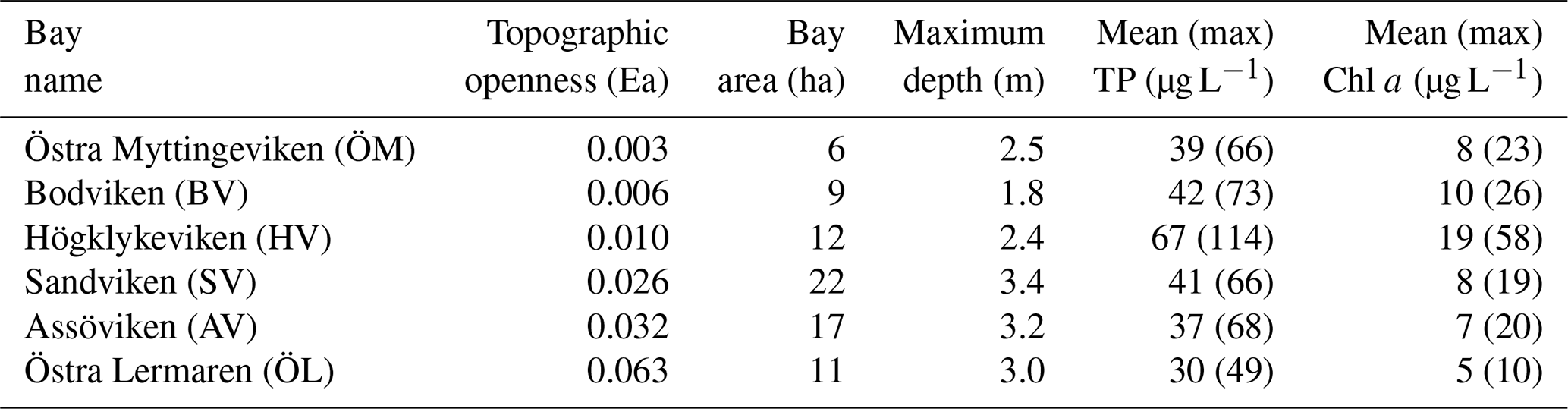
Furthermore, longer water retention times in the more enclosed bays lead to accumulation of nutrients and higher chlorophyll-a concentrations than in semi-open bays. It is noteworthy that Högklykeviken (HV) had significantly higher total phosphorus and chlorophyll-a concentrations than the other bays (see Table 1). Högklykeviken represents a system that has shifted from benthic vegetation dominance to plankton dominance after an extensive dredging of the opening area. The bay is subjected to a restoration measure since May 2024 (after our initial measurements in April). The restoration has consisted of an aluminum-based geoengineering treatment to decrease internal load of phosphate from the sediment (Rydin et al., 2025). All study bays were small (6 to 22 ha) and shallow (1.8–3.4 m, see Table 1), though the more open bays were slightly deeper than enclosed ones.

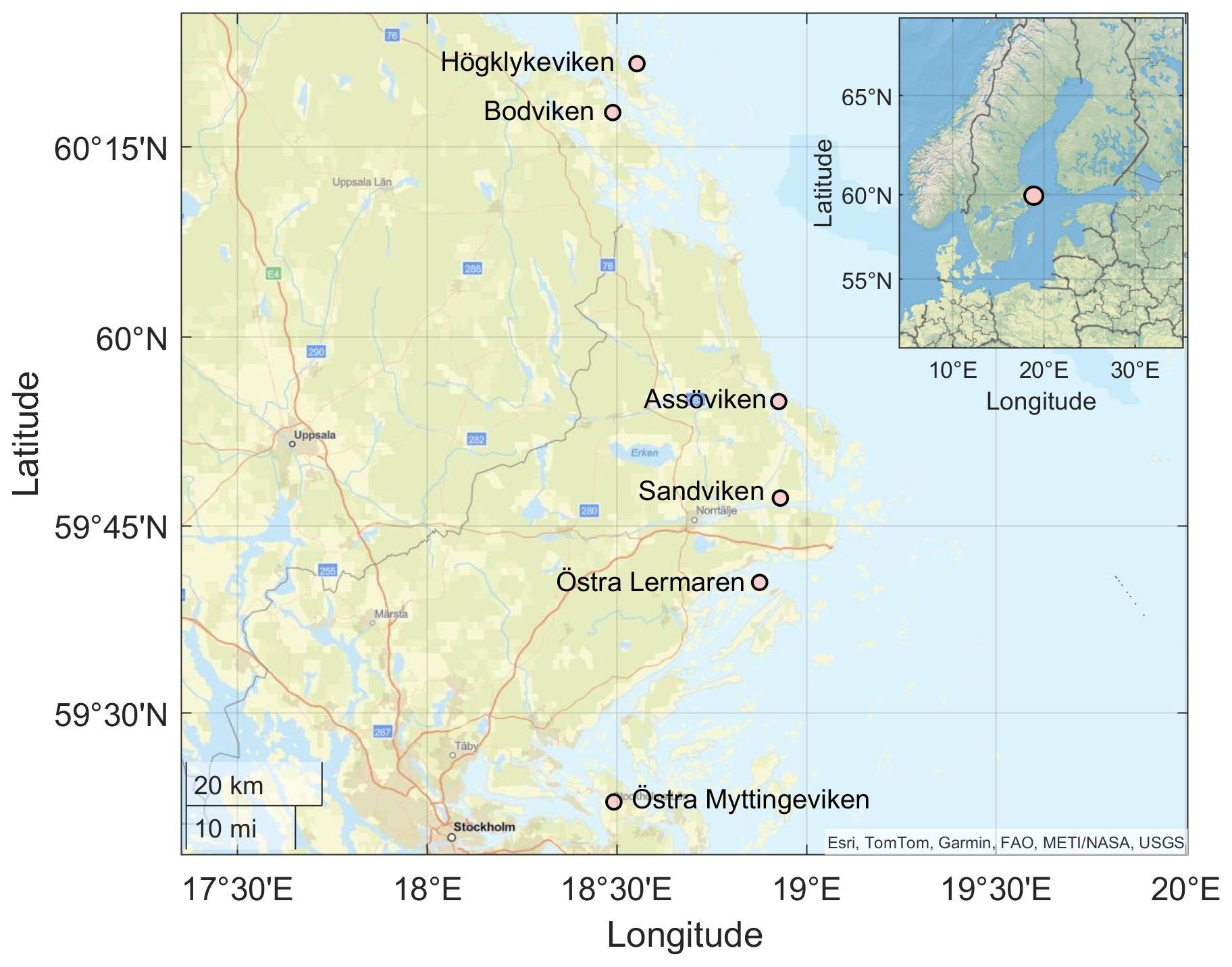
Figure 1 Location of the sampling bays in the wider Stockholm Archipelago in the Western Baltic Sea. Basemap data: Esri, TomTom, Garmin, FAO, METI/NASA/NOAA, USGS | Powered by Esri.

Table 1 Characteristics of the six study bays, including topographic openness index (Ea), physical dimensions, and the eutrophication indicators phosphorus and chlorophyll concentrations in seawater. Mean and maximum total phosphorus (TP) and chlorophyll a (Chl a) concentrations represent historical data from 4 to 7 sampling occasions per year during 2020–2024 (spring through autumn) and were used to characterize eutrophication status for bay selection. Bodviken (BV) was not sampled in 2020; Östra Lermaren (ÖL) not sampled in 2022–2023, the other bays were sampled all years.

2.2 Continuous measurements of GHG concentrations

Measurements were conducted during midday in April and September/October 2024 from a small boat. A cavity ring-down spectrometer (CRDS, model Picarro G2508, Picarro Inc., USA) coupled with a custom-built water equilibration gas analyzer system (WEGAS) was used to measure the concentrations of atmospheric and dissolved CO₂, CH₄ and N₂O. The instrument was factory-calibrated by the manufacturer in 2022, and the measurements presented here represent its first field deployment following calibration. According to the manufacturer’s specifications, the precision of 1-minute averaged measurements is <300 ppb + 0.05 % of reading for CO₂, <7 ppb + 0.05 % for CH₄, and <10 ppb + 0.05 % for N₂O. The CRDS technique is characterized by negligible instrumental drift which was confirmed by a post-campaign calibration (0.2 % for CO₂ and −0.5 % for CH₄ over three years since the last calibration). The offset determined by the post-campaign calibration was significantly smaller than the concentration ranges sampled in this study (−0.4 ppm for CO₂ and 0.03 ppm for CH₄ in April; −1.2 ppm CO₂ and 0.04 ppm CH₄ in September). Given that the study focuses on relative spatial and seasonal differences measured with the same instrument, such a small systematic offset would not affect the interpretation of the results. April measurements in Bodviken were conducted using a Picarro G2201-i instead of the G2508, which measured the concentrations of CO₂ and CH₄ but not N₂O.

2.2.1 The WEGAS system

The WEGAS system is described in detail in Humborg et al. (2019). Briefly, seawater from just below the surface (at approximately 30 cm depth) was continuously passed through a water handling system consisting of a thermosalinograph (SBE45 MicroTSG, Seabird Scientific, US) measuring seawater temperature, salinity, and conductivity; a flowmeter maintaining stable flow at ∼3 L min⁻¹; and a showerhead equilibrator (RAD-AQUA, Durridge, US). After the seawater was equilibrated with a flow of ambient air, the air stream was passed through a custom-built cryocooler that cooled the gas to a dew point of 4 °C to reduce excess humidity before analysis by the CRDS. A gas handling system controlled airflow switching between ambient air measurements and equilibrator measurements. Each sampling cycle consisted of 5 min of ambient air followed by 40 min of equilibrator air, with cycles repeated until horizontal profiling of each bay was completed. Transition periods between ambient and equilibrator air were excluded from analysis. Sampling durations lasted between 60 and 90 min (typically ∼ 75 min). Measurements were conducted both inside and outside bay areas. To distinguish between “inner bay” and “outer bay” sampling points, we delineated the bay boundary at the narrowest part of the inlet connecting each bay to the open Baltic Sea. This location represents the transition in water exchange, residence time, and mixing characteristics. For cross-bay comparisons, concentrations were first averaged within each bay, and summary statistics (e.g., median) were then calculated across bays using one value per bay, treating each bay as an independent unit rather than applying area-weighted averaging.

2.2.2 Gas concentration calculations

Mole fractions (ppm) of CO₂ were converted to partial pressures (µatm) using the Seacarb (v.3.3) x2pCO2 function (Gattuso et al., 2021). Mole fractions (ppm) of CH₄ and N₂O were converted to molar concentrations using Henry's law (Eq. 1), assuming full equilibration in the equilibrator at ambient pressure:

$$\begin{array}{}\text{(1)}& C=p\times K_{\mathrm{H}}\end{array}$$

where C is concentration (mol L⁻¹), p is the partial pressure (1 ppmv corresponds to 1 µatm at an ambient pressure of 1 atm), and K_H is the temperature-corrected Henry's law constant:

$$\begin{array}{}\text{(2)}& K_{\mathrm{H}}=K_{\mathrm{H}}^{*}\times \exp \left({\displaystyle \frac{-{\mathrm{\Delta }}_{\mathrm{sol}}H}{R}}\times \left({\displaystyle \frac{\mathrm{1}}{T_{\mathrm{K}}}}-{\displaystyle \frac{\mathrm{1}}{\mathrm{298.15}\mathrm{K}}}\right)\right).\end{array}$$

where $K_{\mathrm{H}}^{*}$ is the Henry's law constant at reference temperature (298.15 K), Δ_solH is the enthalpy of dissolution, R is the gas constant and T_K is water temperature in Kelvin. Constants were obtained from Sander (2015).

Gas solubilities were calculated using the Bunsen solubility coefficient:

$$\begin{array}{}\text{(3)}& \begin{array}{rl}\mathit{\beta }& =\exp \left(A_{\mathrm{1}}+A_{\mathrm{2}}\left({\displaystyle \frac{\mathrm{100}}{T}}\right)+A_{\mathrm{3}}\ln \left({\displaystyle \frac{T}{\mathrm{100}}}\right)\right.\\ & \left.+S\left(B_{\mathrm{1}}+B_{\mathrm{2}}\left({\displaystyle \frac{T}{\mathrm{100}}}\right)+B_{\mathrm{3}}{\left({\displaystyle \frac{T}{\mathrm{100}}}\right)}^{\mathrm{2}}\right)\right)\end{array}\end{array}$$

where β is the dimensionless Bunsen coefficient, A₁–A₃ and B₁–B₃ are gas-specific constants from Wiesenburg and Guinasso Jr (1979), T is temperature (K), and S is salinity (g kg⁻¹). For N₂O, the solubility constant is given by K₀=β, whereas for CH₄ – assuming ideal gas behaviour – the solubility constant is calculated as K₀=β (R×273.15 K).

2.2.3 Air-sea flux calculations

Air-sea fluxes of GHGs were estimated using:

$$\begin{array}{}\text{(4)}& F=k\times K_{\mathrm{0}}\times (p{X}_{\mathrm{seawater}}-p{X}_{\mathrm{air}}).\end{array}$$

where F is flux, k is gas transfer velocity (m s⁻¹), K₀ is solubility, and pX represents partial pressures in seawater and air. The gas transfer velocity was calculated following Cole and Caraco (1998) which is representative for lake environments:

$$\begin{array}{}\text{(5)}& k=(\mathrm{2.07}+\mathrm{0.215}\times U_{\mathrm{10}}^{\mathrm{1.7}})\times {\left({\displaystyle \frac{Sc}{\mathrm{600}}}\right)}^{-\mathrm{0.5}}.\end{array}$$

where U₁₀ is wind speed and Sc is the Schmidt number. Schmidt numbers for brackish Baltic Sea conditions were interpolated between freshwater and seawater values (Wanninkhof, 2014):

$$\begin{array}{}\text{(6)}& Sc=(S{c}_{\mathrm{seawater}}-S{c}_{\mathrm{freshwater}})\times {\displaystyle \frac{S}{\mathrm{35}}}+S{c}_{\mathrm{freshwater}}.\end{array}$$

Wind speed at 10 m height was obtained from the ICON-EU numerical weather prediction model (Deutscher Wetterdienst, Germany). Model output at ∼ 7 km horizontal resolution was accessed through the Ventusky online visualization platform (https://www.ventusky.com, last access: 25 February 2026). We extracted 10 m wind values corresponding to the sampling dates and coordinates of each site. The derived wind speeds were 1.67 m s⁻¹ (Sandviken), 7.0 m s⁻¹ (Assöviken), 6.67 m s⁻¹ (Högklykeviken), and 4.4 m s⁻¹ (Bodviken) in April; 3.3 m s⁻¹ (Sandviken), 3.9 m s⁻¹ (Assöviken), 7.2 m s⁻¹ (Högklykeviken), and 3.6 m s⁻¹ (Bodviken) in September; and 2.5 m s⁻¹ in both Östra Lermaren and Östra Myttingeviken in October.

2.2.4 CO₂-equivalent fluxes

To derive CO₂-equivalent fluxes, calculated fluxes (µmol m⁻² d⁻¹) were converted to mass units (mg m⁻² d⁻¹) using respective molar masses, then multiplied by 100-year sustained global warming potentials of 45 for CH₄ and 270 for N₂O (Neubauer and Megonigal, 2015).

2.3 Collection and analysis of seawater and sediment samples

2.3.1 Water sample collection and laboratory analysis

Surface water samples (0–1 m depth) were collected from the centre of each bay and kept cool until analysis at the certified Erken laboratory, Uppsala University (ISO/IEC 17025). Dissolved concentrations of nitrite-N and nitrate-N (NO₂-N + NO₃-N, SIS, 1996), ammonium-N (NH₄-N, SIS, 2005) and phosphate-P (PO₄-P, SIS, 2004) were determined colorimetrically using an AutoAnalyzer 3 (SEAL Analytical, US) or a U-2910 analyser (Hitachi, Japan). Total nitrogen (TN, SIS, 1996) and phosphorus (TP, SIS, 2004) concentrations were determined as NO₃-N and PO₄-P after persulfate digestion.

Chlorophyll a (Chl a) was determined spectrophotometrically after acetone extraction (SIS, 1980). Total organic carbon (TOC, SIS, 2024) was analyzed using a 680 °C combustion catalytic oxidation method with a TOC-L analyser (Shimadzu, Japan). Organic content was estimated as loss on ignition (LOI) after combustion at 550 °C (SIS, 1983). Turbidity was measured as Formazin Nephelometric Units (FNU, SIS, 2016) using a 2100 P ISO turbidity meter (Hach, CO, USA).

2.3.2 In-situ water measurements

Temperature, salinity and dissolved oxygen were measured using a WTW Multi 3420 probe (Xylem, US), and pH was measured with a YSI Pro10 pH meter (Xylem, US). All measurements were taken in the centre of each bay, adjacent to the water sampling location.

2.3.3 Vegetation surveys

Aquatic vegetation cover was recorded in all basins by a free-diver in August, a few weeks prior to the September GHG measurements. For two bays (Högklykeviken and Bodviken), vegetation cover was also estimated in May, a few weeks after the April GHG measurements. For the other two bays with GHG measurements in May (Assöviken and Sandviken), we retrieved May vegetation data from a previously conduced survey (in 2022). Survey sites consisting of 7–13 circular areas (5 m radius, ∼80 m²) were distributed evenly from the bay opening to the innermost areas. Survey sites were randomly allocated within subareas along a distance-from-opening gradient, excluding nearshore areas with <0.5 m water depth. Within each survey site, percentage cover of individual taxa and total cover of all macroscopic autotrophs (including filamentous algae and cyanobactera) was visually estimated. The vegetation assessment method follows a standardized national protocol that has been widely applied in this region (e.g., Hansen et al., 2019). For this study, we used two vegetation indicators: (1) total vegetation cover and (2) cumulative cover of all rooted vegetation (sum of all rooted taxa cover) because they capture distinct functional aspects of benthic vegetation that are relevant for greenhouse-gas dynamics. Total vegetation cover provides an integrated measure of overall primary producer abundance, which can influence water-column oxygen dynamics and carbon cycling through photosynthesis and respiration. Rooted vegetation cover specifically reflects the presence of macrophytes capable of affecting sediment–water exchange processes through below-ground gas transport in addition to photosynthesis and respiration. These indicators therefore represent the most ecologically meaningful metrics for assessing vegetation-related controls on GHG concentrations in these shallow bays.

2.3.4 Sediment sampling and analysis

Sediment cores were collected using a gravity corer (63 mm inner diameter) and sectioned on-site immediately upon return to land. For this study, we used only data from the uppermost sediment layer (0–1 cm), which represents the sediment-water interface where redox-sensitive processes and exchanges directly influence surface-water GHG concentrations. We note that deeper sediment layers may be important for methane production and ebullition dynamics, but were beyond the scope of the present study. Sediment samples were homogenized in sterile containers and transferred to pre-weighed polypropylene vials for analysis. Samples were freeze-dried and pulverized to fine powder. Porosity was calculated from weight loss after freeze-drying, assuming a sediment dry density of 2.65 g cm⁻³ (Burdige, 2006). Sediment water content was determined after freeze-drying, and organic content was determined by loss on ignition (LOI) at 550 °C for 2 h (U.S. Environmental Protection Agency, 1971). Organic carbon (C_org) and nitrogen (N_org) content were determined using an Elemental Combustion System (ECS 4010, Costech Analytical Technologies Inc, US).

3 Results and Discussion

3.1 Spatio-temporal variability of GHG across shallow bays

Surface water concentrations of CH₄, pCO₂, and N₂O exhibited substantial spatial and temporal variability across the six study bays, between seasons, and between areas inside and outside the bays (see Figs. 2 and A1–A6 in the Appendix). Statistical analysis using Kruskal-Wallis tests (based on 10 % of the data to avoid interdependence between neighbouring measurement points) confirmed significant differences in GHG concentrations between bays (see Table A1 in the Appendix). Calculating post-hoc Bonferroni corrected p-values allowed us to discern which bays differed from each other (see Table A2). A Wilcoxon rank-sum test further showed significant differences between inside and outside bay areas for all gases (see Table A3).

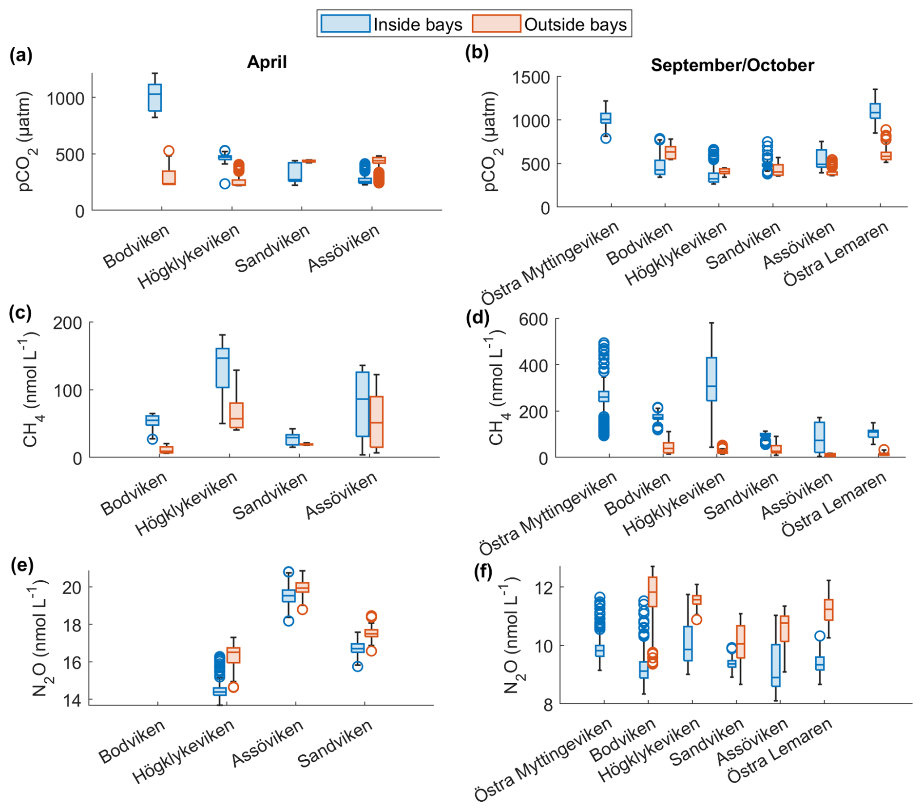
Figure 2 Spatial variation of surface water concentrations of (a–b) CO₂, (c–d) CH₄ and (e–f) N₂O across six shallow bays in April and September/October 2024. Box plots show median, quartiles, outliers and range for measurements inside (blue) and outside (red) each bay. N₂O data were not available for Bodviken, and no outside measurements were obtained for Östra Myttingeviken in October. Bays are arranged from left to right in increasing order of topographic openness.

3.1.1 CO₂ concentrations

CO₂ was generally close to saturation in surface waters (see Table 2), with concentrations differing significantly between bays (see Fig. 2 and Tables 2 and A1). The highest concentrations were observed in Bodviken in April (mean 1022 ± 121.6 ppm) and in Östra Lermaren and Östra Myttingeviken in October (mean 1108 ± 117.7 ppm and 1033 ± 83.1 ppm, respectively). These bays showed significantly higher CO₂ concentrations inside compared to outside areas (see Table A2). In contrast, bays where CO₂ was near saturation showed no significant inside–outside differences. Overall, no consistent patterns emerged across the bay openness gradient or between inside versus outside areas across all bays and seasons.

Previous studies from the Tvärminne archipelago in southwestern Finland reported values that were of a similar magnitude or exceeded the concentrations measured in our study: 750 ppm (Humborg et al., 2019), 4.5–13,100 ppm (Asmala and Scheinin, 2024), and 160–2521 ppm (Geilfus et al., 2025). Long-term measurements across the open Baltic Sea, that were conducted on the Finnmaid ferry between Travemünde and Helsinki (Bittig et al., 2023), reported values ranging between 18–1238 µatm (mean 293 ± 60 µatm) in April and 14–1198 µatm (mean 375 ± 50 µatm) in September. Similar measurements by Schneider et al. (2014) yielded values of <200 µatm in summer and ∼ 400 µatm in September. Notably, maximum values in our study compared well with the maximum values reported in Bittig et al. (2023) as well as the mean concentrations of 1288 ppm reported from Swedish lakes (Humborg et al., 2010). The sheltered nature of the bays may resemble lake-like conditions with respect to air–water CO₂ exchange, but not necessarily other gases.

These findings suggest that although shallow bays often accumulate organic matter and are significant reservoirs of carbon and nutrients accumulated from surrounding areas (Gubri et al., 2025; Wikström et al., 2025), their role in atmospheric CO₂ exchange is not uniform. Instead, they may function either as CO₂ sources or sinks depending on seasonal conditions and bay-specific properties such as openness, vegetation cover, and eutrophication status. However, our measurements represent only snapshots from two seasons and capture transitional states rather than peak or minimum seasonal conditions. In temperate coastal environments, growth of phytoplankton and algae in spring reduces pCO₂ in the water column, while biomass decay in autumn results in elevated pCO₂. Recent studies by Honkanen et al. (2021) and Pönisch et al. (2025) reported diurnal variability in surface-water pCO₂ and CH₄ in the Baltic Sea that could be linked to biological and physical drivers such as solar radiation, temperature or biological activity. We acknowledge that our measurements, which were always conducted around noon, do not capture these diurnal fluctuations and thus likely introduce a small but systematic bias relative to true daily mean conditions. While such measurements remain valuable, more extensive, long-term monitoring is required to identify the environmental parameters that drive these systems to function as CO₂ sources or sinks across different temporal scales.

3.1.2 CH₄ concentrations

CH₄ was strongly supersaturated in all study bays (see Table 2) and significantly higher inside bays compared to open water (see Fig. 2 and shown using a Wilcoxon rank-sum test, see Table A2 in the Appendix). Concentrations were generally higher in autumn compared to spring (see Fig. 2c, d and Table 2), likely reflecting enhanced organic matter degradation and increased activity of methanogenic archaea in anoxic sediments (Conrad, 2009). The highest concentrations were recorded in Högklykeviken, reaching 181 nmol L⁻¹ in April and 580 nmol L⁻¹ in September. Östra Myttingeviken also showed elevated levels up to 494 nmol L⁻¹. Both are enclosed bays, with Högklykeviken representing a more disturbed system that has shifted from benthic vegetation dominance to plankton dominance.

CH₄ production occurs primarily through methanogenic archaea in oxygen-depleted sediments (Schubert and Wehrli, 2019). In enclosed bays with narrow openings, limited water exchange minimizes sediment disturbance by waves and currents, allowing organic matter to accumulate (Gubri et al., 2025) and creating conditions conducive to elevated CH₄ production (Egger et al., 2016). Recent studies have shown that such shallow, sheltered bays are significant organic carbon reservoirs, with higher accumulation correlated with vegetation cover, coastal morphology, and landscape characteristics (Wikström et al., 2025).

Another factor that can contribute substantially to CH₄ emissions in shallow, organic rich sediments is ebullition (McGinnis et al., 2006; Hermans et al., 2024; Bisander et al., 2025). Recently, Bisander et al. (2025) showed that ebullition from sandy sediments can be substantial. The WEGAS system measures CH₄ from both benthic diffusion and bubble dissolution. Consequently, the observed CH₄ concentrations represent the combined effect of these pathways, and without isotopic information we cannot distinguish between diffusive transport and ebullition. Although no visible bubbling was observed during sampling, we cannot exclude the possibility that episodic ebullition events might have impacted our measurements. This measurement limitation should be considered when interpreting the relationships between CH₄ and the environmental parameters described in Sect. 3.1.4.

Our measured concentrations are comparable to previous studies in the Baltic Sea region. Studies in the southern Stockholm Archipelago around Askö reported 6–460 nmol L⁻¹ (Roth et al., 2022) and 26–6596 nmol L⁻¹ (Lundevall-Zara et al., 2021), while studies from the southwestern coast of Finland reported ranges of 19–469 nmol L⁻¹ (Geilfus et al., 2025), 44 nmol L⁻¹ (Humborg et al., 2019), 130–665 nmol L⁻¹ (Myllykangas et al., 2020), and 0–6767 nmol L⁻¹ (Asmala and Scheinin, 2024). The CH₄ concentrations measured in our study are significantly higher than values reported from long-term measurements in the open Baltic Sea, ranging between 3.5–6 nmol L⁻¹ (Schneider et al., 2014), 2.8–18.6 nmol L⁻¹ (Jacobs et al., 2021) and 3.2–22 nmol L⁻¹ (Gülzow et al., 2013). The consistent observation of high spatial variability and local CH₄ hotspots across these studies underscores the need for high-resolution sampling to accurately characterize GHG dynamics in shallow coastal ecosystems.

3.1.3 N₂O concentrations

N₂O concentrations showed pronounced seasonal variation, with higher values in spring (13.7–20.8 nmol L⁻¹) than in autumn (8–11.75 nmol L⁻¹). Most bays were slightly subsaturated or close to saturation (see Table 2). In April, N₂O concentrations were higher in open bays compared to more enclosed bays (see Fig. 2e), while no such trend was apparent in the September data. In addition, N₂O concentrations were generally higher outside bays than inside, contrasting with the patterns observed for CH₄.

The consistently higher N₂O concentrations outside the bays may be explained by hydrodynamic and sedimentological conditions that favour coupled nitrification-denitrification (Marchant et al., 2016). Higher water currents enhance oxygen penetration into coarser sediments (sand, gravel, stones) which promotes nitrification in the oxic surface layer and denitrification in underlying anoxic microzones (Murray et al., 2015). Lower concentrations inside bays are likely the result of reduced water currents and the accumulation of fine organic matter. These conditions promote weaker ventilation, stronger sediment–water coupling, and lower oxygen availability, which tend to suppress nitrification and favour complete denitrification to N₂ rather than N₂O, ultimately reducing dissolved N₂O concentrations. Additionally, higher N₂O concentrations outside the bays may partly reflect wind-induced mixing in the more exposed areas, where longer fetch and higher wind speeds enhance vertical exchange and stimulate nitrification–denitrification dynamics. In contrast, the sheltered bay interiors experience reduced wind forcing, limiting mixing and potentially suppressing N₂O production and release.

Few studies have simultaneously measured CO₂, CH₄ and N₂O in shallow Baltic Sea bays. Our results are similar to those of Geilfus et al. (2025), who reported concentrations of 9–25 nmol L⁻¹ in August/September 2023. Seasonal patterns in dissolved N₂O observed in our shallow Baltic Sea bays, with relatively high concentrations in spring (April) and lower concentrations in autumn (September/October), are consistent with patterns reported from other Baltic coastal settings. Long term observations in the Kiel Bay (Boknis Eck time series station in Eckernförde Bay) likewise show elevated N₂O in winter and early spring followed by reduced concentrations in autumn, particularly under hypoxic or anoxic conditions (Ma et al., 2019). At that site, seasonal declines in dissolved oxygen and nutrient dynamics were closely coupled to N₂O variability, with lower autumn N₂O attributed to increased denitrification to N₂ under suboxic conditions that consume N₂O (Ma et al., 2019). Likewise, Cheung et al. (2025) identified pronounced seasonal N₂O variation in coastal Baltic waters and linked it to shifts in redox conditions and stratification that modulate microbial nitrification and denitrification pathways–processes that are both oxygen sensitive and seasonally dynamic. In shallow bays, spring mixing and higher oxygen availability may enhance nitrification and partial denitrification, leading to relatively elevated N₂O, whereas prolonged summer stratification and oxygen depletion in late summer and early autumn favour complete denitrification and N₂O consumption, resulting in lower observed N₂O concentrations. These seasonally varying oxygen and nitrogen transformation dynamics offer a plausible mechanistic framework for the spring–autumn N₂O trend observed in our study.

Table 2 Mean concentrations (averaged over inside or outside bay area), ranges, and saturation percentages of CH₄, CO₂, and N₂O inside and outside of six bays in spring and autumn.

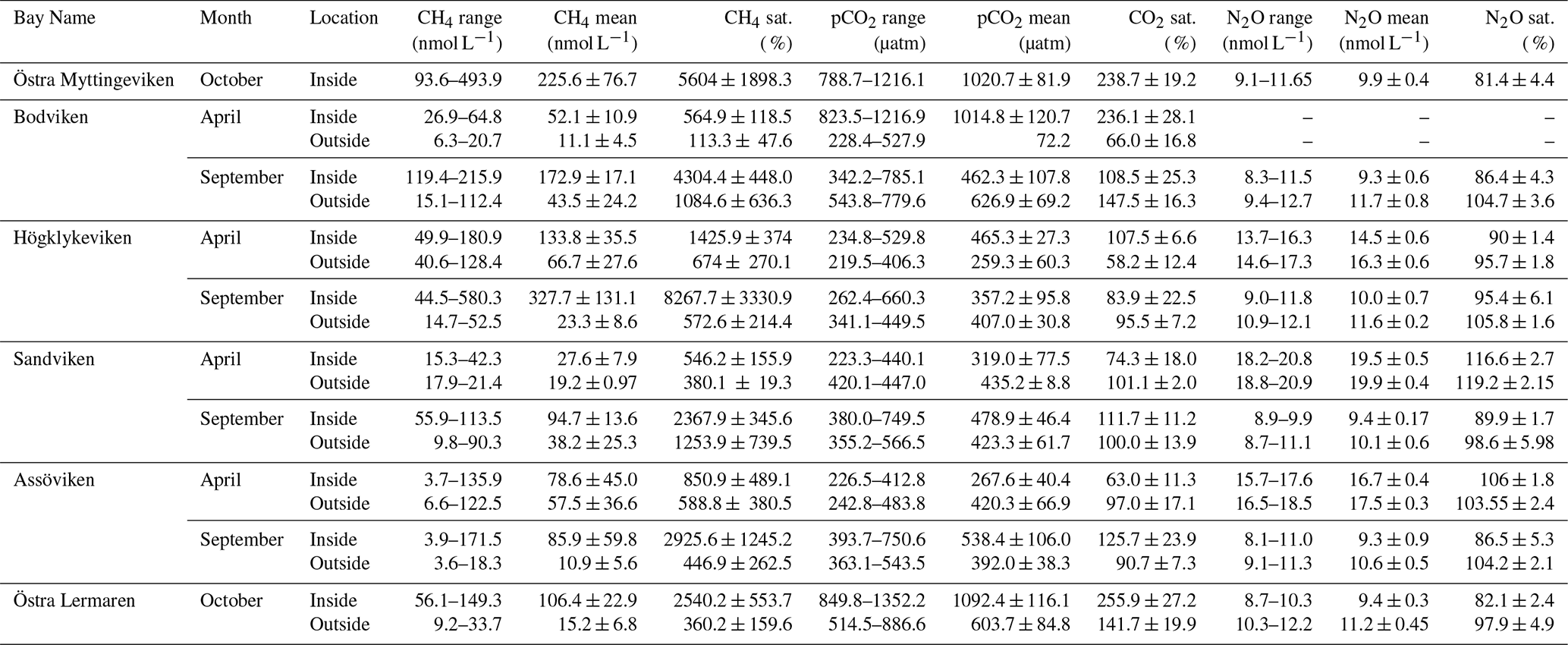
Table 3 Seawater properties in the different bays in spring and autumn, including seawater temperature (T_SW), salinity (S), dissolved oxygen at seafloor, chlorophyll-a (Chl-a) concentration, turbidity, pH, total organic carbon (TOC), loss of ignition (LOI) as well as dissolved concentrations of total phosphorus (TP), phosphate (PO₄), total nitrogen (TN), nitrite and nitrate (NO₂ + NO₃).

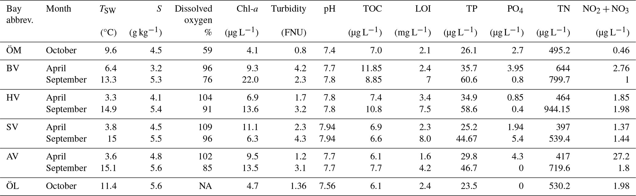
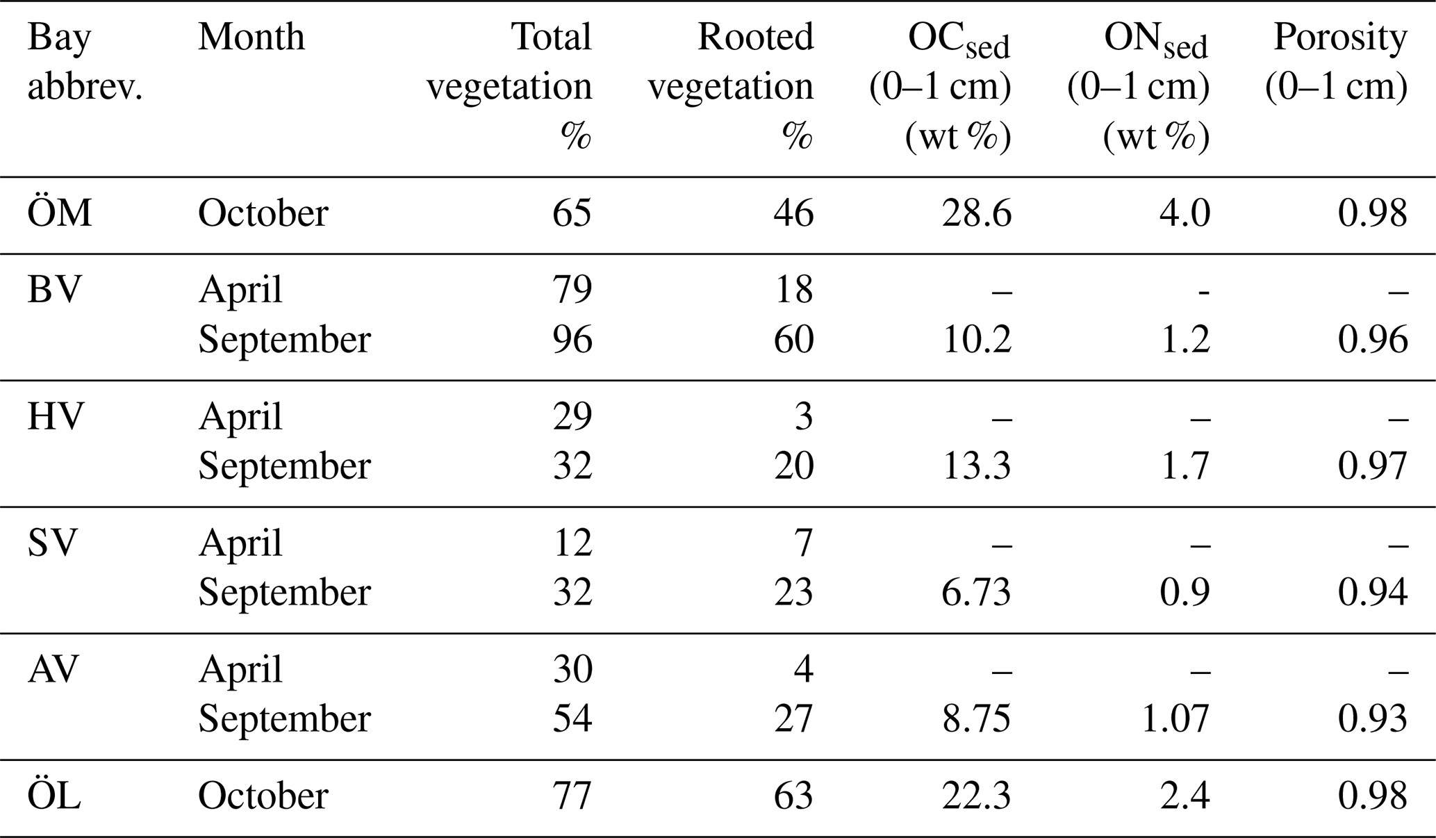
Table 4 Sediment and vegetation properties in the different bays in spring and autumn including the total cover of aquatic vegetation, cumulative cover of rooted vegetation, organic carbon (OC_sed) and organic nitrogen ON_sed in the sediment and sediment porosity.

3.1.4 Correlation of surface water GHG concentrations with environmental parameters across bays

To identify environmental factors associated with variability in surface-water GHG concentrations, we conducted a Spearman’s rank correlation analysis using bay-averaged GHG concentrations and environmental parameters measured in the center of each bay (see Fig. 3 as well as Figs. A7 and A8 in the Appendix). To increase statistical power and assess general trends, data from April and September/October were pooled.

CO₂ concentrations were positively correlated with LOI (r=0.67, p=0.04) and showed negative correlation trends with chlorophyll-a ($r=-\mathrm{0.64}$, p=0.05) and pH ($r=-\mathrm{0.59}$, p=0.07), as well as a positive correlation trend with rooted vegetation cover (r=0.60, p=0.06). The negative relationship with chlorophyll-a and pH suggests that periods or locations of enhanced primary production are associated with CO₂ drawdown and elevated pH, whereas positive correlations with LOI and vegetation indicate that respiration and mineralization of organic matter – particularly from macrophyte-derived inputs – can offset photosynthetic uptake and elevate CO₂ concentrations in surface waters. This interpretation is supported by the observation that the bays with the highest CO₂ concentrations (Östra Lermaren, Östra Myttingeviken, and Bodviken) shared extensive rooted vegetation cover and elevated sediment organic carbon content. In Östra Lermaren and Östra Myttingeviken, which also exhibited the lowest eutrophication status as measured by TP and chlorophyll-a concentrations, high CO₂ concentrations may appear counter-intuitive but are likely driven by substantial autochthonous organic matter inputs from decaying vegetation, consistent with coastal studies documenting seasonal CO₂ hotspots linked to remineralization of organic-rich material (Amaral et al., 2021; Asmala and Scheinin, 2024). In contrast, Bodviken combined high CO₂ concentrations with comparatively higher eutrophication, suggesting that enhanced internal mineralization under nutrient-rich conditions may dominate CO₂ production in this system. Although the correlations with pH and rooted vegetation were slightly above the conventional 5 % significance threshold, they are consistent with the expected coupling between primary production, organic matter mineralization, and CO₂ dynamics in shallow coastal systems. Given the limited number of bays, these trends should be interpreted as exploratory and warrant confirmation through studies with higher spatial and temporal resolution.

CH₄ concentrations showed a significant negative correlation with dissolved oxygen ($r=-\mathrm{0.75}$, p=0.03) and a positive correlation with LOI (r=0.67, p=0.04). These relationships are consistent with enhanced methanogenesis under low-oxygen conditions and increased availability of degradable organic substrates in the water column, which together promote CH₄ production and accumulation.

In contrast, N₂O concentrations exhibited significant negative correlations with temperature ($r=-\mathrm{0.82}$, p=0.01), TN ($r=-\mathrm{0.72}$, p=0.04), total vegetation cover ($r=-\mathrm{0.71}$, p=0.04), and rooted vegetation ($r=-\mathrm{0.78}$, p=0.02). The negative relationship of N₂O and temperature is likely driven by two key factors: (1) increased N₂O solubility at lower temperatures, and (2) the temperature sensitivity of denitrification enzymes. Under low-temperature conditions, enzymatic activity of N₂O reductase may be reduced, potentially slowing conversion of N₂O to N₂ and thereby increasing net N₂O emissions (Wang et al., 2014). In addition, vegetation-driven oxygenation of surface sediments can both increase and decrease N₂O production by shifting the balance between nitrification and denitrification. While oxygenation can stimulate nitrification near roots and dentrification in adjacent anoxic zones (e.g. Nyer et al., 2022), sustained and strong oxygenation can surpress denitrification and lead to more complete reduction to N₂ thereby lowering N₂O fluxes (Murray et al., 2015). Contrary to findings reported by Murray et al. (2015), we could not observe a correlation between the concentrations of NO₂ + NO₃ and N₂O across the bays. This decoupling likely reflects the dominance of local-scale processes characteristic of shallow, sheltered bay environments. In particular, N₂O production may be spatially decoupled from water-column NO_x concentrations if it occurs primarily in sediments, where nitrate availability, redox gradients, and organic matter supply differ substantially from overlying waters. In organic-rich bay sediments, denitrification may proceed efficiently to N₂, thereby limiting N₂O accumulation despite elevated NO_x in the water column. In addition, rapid biological uptake of inorganic nitrogen by phytoplankton and benthic vegetation can reduce ambient NO${}_{\mathrm{2}}^{-}$ + NO${}_{\mathrm{3}}^{-}$ concentrations without proportionally affecting N₂O production. Physical processes such as advection, sediment–water exchange, and episodic ebullition may further bypass water-column NO_x controls on dissolved N₂O. Finally, differences in spatial scale, environmental setting, and sampling strategy between this study and the global synthesis of Murray et al. (2015) likely contribute to the contrasting relationships observed.

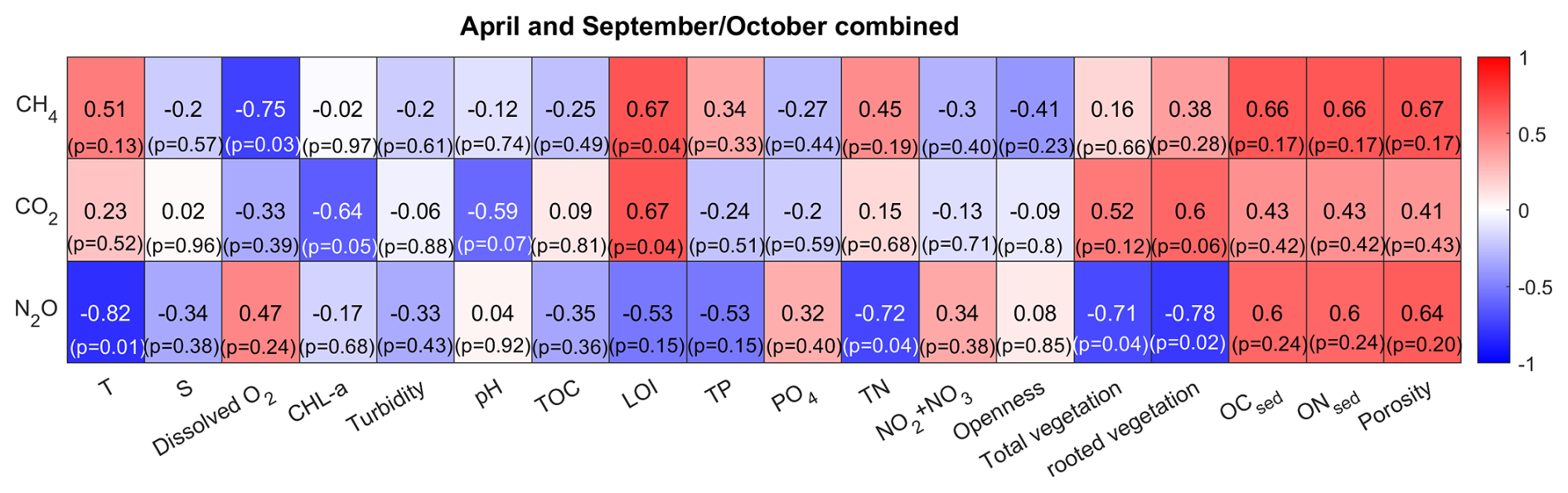
Figure 3 Spearman correlation matrix between environmental parameters and CH₄, CO₂ and N₂O for data pooled from April and September/October. Blue indicates a negative correlation, red indicates a positive correlation. Significance (at the 95 % confidence level) is indicated by p-values.

3.1.5 Correlation between N₂O and CH₄

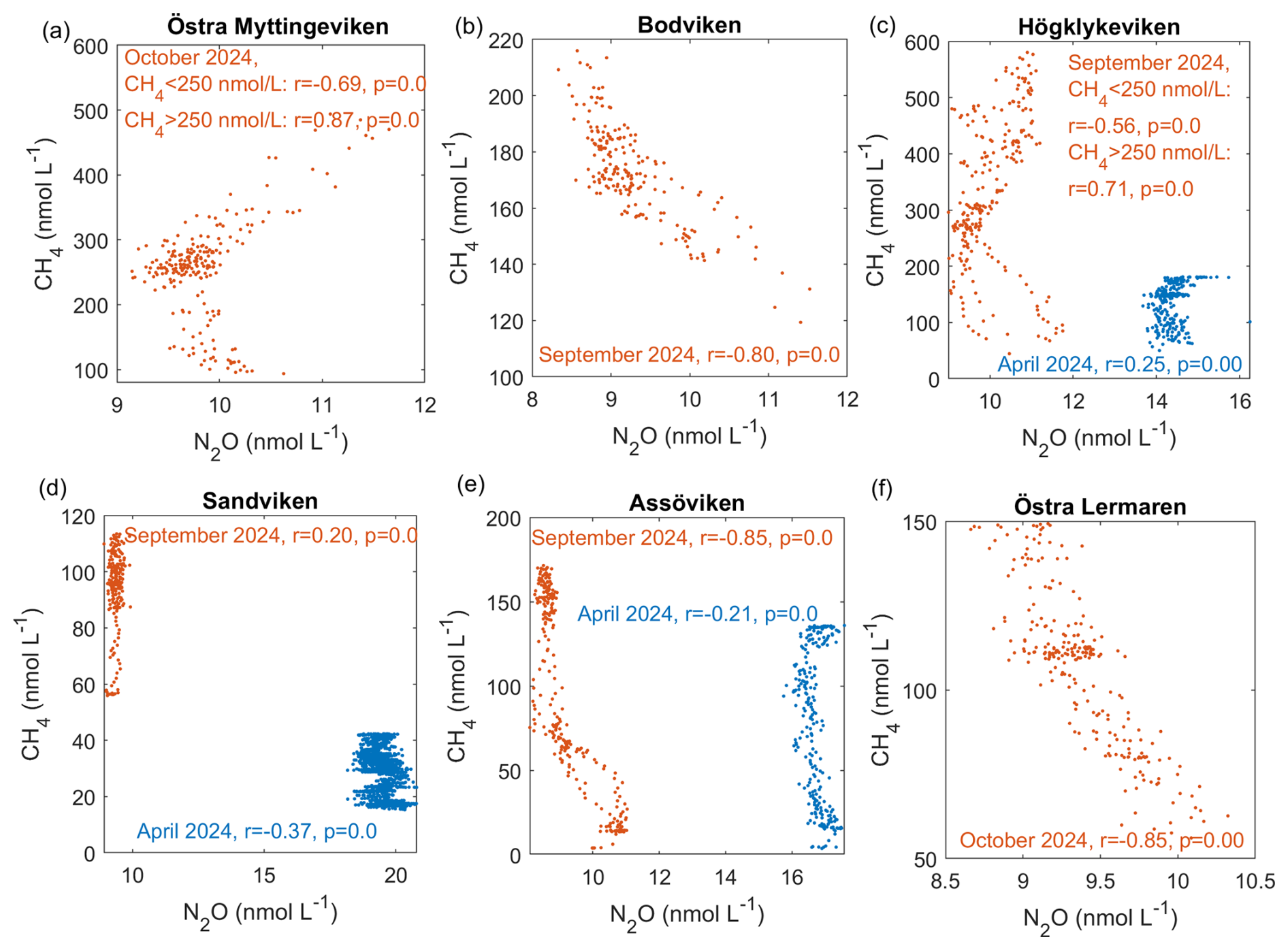
Negative correlations between N₂O and CH₄ were observed across different bays and seasons (see Fig. 4). A similar negative correlation was reported by Woszczyk and Schubert (2021).

This negative correlation can be likely explained by the spatial distribution of the gases. N₂O concentrations were generally highest outside the bays and in the channels that connect to the open sea, where the water current velocities are higher and coarser substrates (sand, gravel, stones) dominate. This pattern is consistent with previous observations that N₂O hotspots often occur in hydrodynamically energetic settings, where strong currents, turbulent mixing, and coarse substrates (sand and gravel) enhance oxygen penetration into sediments and stimulate nitrification (Murray et al., 2015). Such conditions also promote rapid porewater–water column exchange, facilitating the release of N₂O produced during coupled nitrification–denitrification. Our elevated N₂O concentrations in channels and outer-bay areas therefore align well with the mechanistic understanding established by earlier studies. In contrast, CH₄ was highest inside the bays, where sedimentary organic matter accumulates in fine muddy sediments.

However, in Högklykeviken and Östra Myttingeviken, the bays with the highest autumn CH₄ concentrations, we observed an interesting shift from negative correlations at CH₄ concentrations <250 nmol L⁻¹ to positive correlations at CH₄ concentrations >250 nmol L⁻¹. This threshold-like behaviour suggests that different biogeochemical processes dominate at high versus low CH₄ concentrations, which is indicative of the complex carbon-nitrogen cycling dynamics of these systems.

The different spatial distributions of CH₄ and N₂O may partly reflect their different optimal oxygen conditions: CH₄ production occurs mainly in anoxic regions, while N₂O production is maximal at suboxic levels where denitrification dominates (Naqvi et al., 2010; Ji et al., 2018; Barnes and Upstill-Goddard, 2018). Although our dissolved oxygen measurements in the central bay locations indicate generally oxic conditions in both Högklykeviken (O${}_{\mathrm{2},\mathrm{dissolved}}=\mathrm{8.3}$ mg L⁻¹ ≈ 91 % saturation) and Östra Myttingeviken (O${}_{\mathrm{2},\mathrm{dissolved}}=\mathrm{5.6}$ mg L⁻¹ ≈ 59 % saturation), we cannot resolve small-scale oxygen heterogeneity and therefore can only speculate that oxygen-reduced microenvironments may existed in areas of high CH₄ concentrations (Briggs et al., 2015). Beyond oxygen availability, several additional mechanisms could explain the shift from a negative to a positive CH₄–N₂O correlation. As mentioned earlier, increased inputs of labile organic matter can stimulate methanogenesis further inside the bays, while changes in the availability of alternative electron acceptors (e.g., nitrate, sulfate, iron) alter competition among metabolic pathways, which can suppress or enhance methanogenesis and modulate N₂O production or consumption. Coupled processes such as nitrate-dependent anaerobic methane oxidation can also link CH₄ and N cycling in non-linear ways (Welte et al., 2016). Ebullition would provide a pathway for CH₄ accumulation by bypassing water-column oxidation and decoupling CH₄ from dissolved N₂O dynamics. However, as mentioned previously, our measurement set-up does not allow us to discern between bubble-mediated and diffusive CH₄. Changes in rooted vegetation and bioturbation may further modify sediment oxygen penetration and bubble release, influencing the relative dominance of CH₄ and N₂O-producing pathways. Finally, sediment disturbance from the research vessel in very shallow areas could explain these anomalous patterns (Liu et al., 2023; Nylund et al., 2025). In order to resolve which of these factors operates in our bays would require targeted process data, limiting our discussion to speculations.

In Högklykeviken, an additional factor may have influenced these relationships. As part of a coastal restoration project, an aluminum-based geoengineering treatment was conducted on 13 May 2024 in the area where both CH₄ and N₂O exhibited high concentrations and positive correlations. This treatment involved injecting an aluminum solution into the sediment to increase the phosphorus retention and reduce eutrophication. Previous research has suggested that aluminium can decrease organic matter remineralization, possibly slowing CH₄ production (Reitzel et al., 2006; Zhou et al., 2018; Scalize et al., 2021). Whether this sediment disturbance altered microbial communities and affected GHG emissions requires further investigation that is beyond the scope of this study.

Figure 4 Correlations between N₂O and CH₄ across different bays and seasons.

3.2 Flux estimates from shallow bays

To determine whether these bays acted as net sources or sinks of GHG, air-sea fluxes were calculated using the methods described in Sect. 2.2. Individual gas flux densities had high variability between bays and seasons.

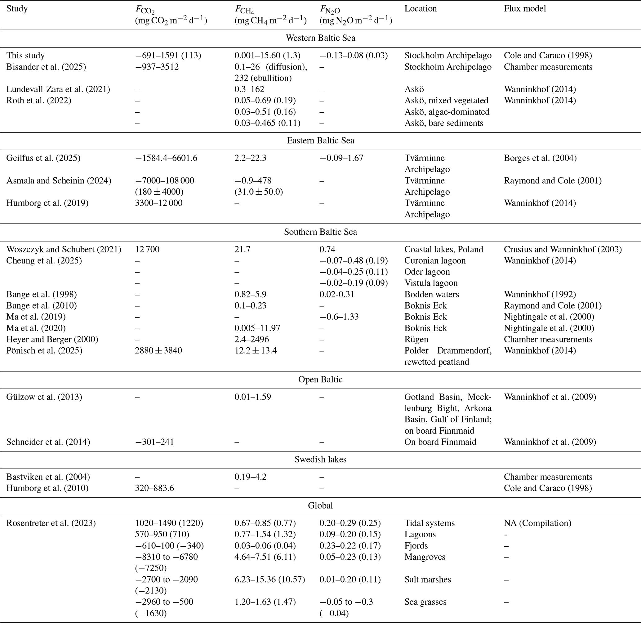
CO₂ flux densities were highly variable ranging from −661 to 1591 mg CO₂ m⁻² d⁻¹ in spring and −526 to 1218 mg CO₂ m⁻² d⁻¹ in autumn. The negative values indicate CO₂ uptake (sinks), while positive values are representative of emissions to the atmosphere (sources). Our estimated CO₂ flux densities are generally at the lower end of values reported from previous studies in the Baltic Sea, Swedish lakes, and global estimates for other coastal habitats (see Table 5).

CH₄ flux densities were generally positive across all bays and seasons and ranged from 0.001 to 15.6 mg CH₄ m⁻² d⁻¹, suggesting that all study sites acted as CH₄ sources. These estimates are similar to those reported for similar habitats by Ma et al. (2019) and fall within a similar range as estimates from several other studies (see Table 5).

N₂O fluxes were small, ranging between −0.13 and 0.08 mg N₂O m⁻² d⁻¹ across bays and seasons.

The more moderate fluxes observed in our study sites compared to other studies likely reflect the sheltered nature of these shallow bays and the relatively low wind speeds we encountered during our measurements. Furthermore, estimates of air–water GHG fluxes are highly sensitive to the choice of gas-transfer velocity parameterization. In this study, we applied the formulation by Cole and Caraco (1998), which was developed for shallow, sheltered, fetch-limited systems and allows for non-zero gas exchange under low wind speeds. This is particularly relevant for the studied bays, which are characterized by weak currents and limited wind-driven turbulence. Alternative parameterizations such as the open-ocean parameterization of Wanninkhof (2014) or the estuarine parameterization of Borges et al. (2004) produce significantly lower or higher estimates, respectively. These differences highlight that absolute flux values are strongly dependent on the assumed turbulence regime and caution against direct inter-study comparisons without careful consideration of the underlying gas-transfer assumptions.

Cole and Caraco (1998)Bisander et al. (2025)Lundevall-Zara et al. (2021)Wanninkhof (2014)Roth et al. (2022)Wanninkhof (2014)Geilfus et al. (2025)Borges et al. (2004)Asmala and Scheinin (2024)Raymond and Cole (2001)Humborg et al. (2019)Wanninkhof (2014)Woszczyk and Schubert (2021)Crusius and Wanninkhof (2003)Cheung et al. (2025)Wanninkhof (2014)Bange et al. (1998)Wanninkhof (1992)Bange et al. (2010)Raymond and Cole (2001)Ma et al. (2019)Nightingale et al. (2000)Ma et al. (2020)Nightingale et al. (2000)Heyer and Berger (2000)Pönisch et al. (2025)Wanninkhof (2014)Gülzow et al. (2013)Wanninkhof et al. (2009)Schneider et al. (2014)Wanninkhof et al. (2009)Bastviken et al. (2004)Humborg et al. (2010)Cole and Caraco (1998)Rosentreter et al. (2023)

Table 5 Range and median values (if available) of flux densities reported from different coastal habitats. NA means “not applicable”.

3.3 CO₂-equivalent fluxes and net greenhouse gas balance

To asses the overall climate impact, individual gas fluxes were converted to CO₂-equivalent fluxes using 100-year sustained global warming potentials of 45 for CH₄ and 270 for N₂O. Total net CO₂-equivalent fluxes, varied significantly between bays and seasons, ranging from −195.2 mg CO₂ eq. m⁻² d⁻¹ (net sink) in Sandviken in Spring to 793.6 mg CO₂ eq. m⁻² d⁻¹ (net source) in Östra Lermaren in autumn, with a median of 131.5 mg CO₂ eq. m⁻² d⁻¹ across all measurements (not area-weighted).

Most bays acted as net GHG sinks in April and net sources in September. However, in Högklykeviken and Bodviken, mean CO2-equivalent fluxes were close to zero and associated with large variability in April, indicating a near-balanced system that alternated between weak sink and source behaviour. Bodviken showed a slightly positive mean flux in both seasons, but the large uncertainty in April suggests that this pattern should be interpreted cautiously. CO₂ fluxes generally dominated the greenhouse gas balance. However, in Högklykeviken, CH₄ emissions nearly balanced CO₂ uptake in spring and even exceeded CO₂ influx in autumn (see Fig. 5 and Table A4 in the Appendix) highlighting the potential importance of CH₄ in disturbed coastal systems. N₂O contributions were generally minor, except in Sandviken in April, where N₂O efflux accounted for 15 % of the net flux. The large variability observed across bays and seasons underscores the challenge of scaling up fluxes from such heterogeneous environments. Nevertheless, to constrain potential regional contributions, we scaled our total CO₂-equivalent fluxes using two area estimates: (1) the total area of shallow, enclosed bays in the archipelagos around Stockholm, Uppsala, Åland and southwestern Finland (142 km², Gubri et al., 2025) as a lower estimate and (2) the total area shallower than 5 m in the Baltic Sea (∼ 30 000 km², Jakobsson et al., 2019; Roth et al., 2022) as an upper estimate. The resulting total carbon fluxes ranged from −7.5 to 30.7 t C d⁻¹ (median 5.1 t C d⁻¹) for the lower limit and −1596 to 6492 t C d⁻¹ (median 1076 t C d⁻¹) for the upper limit. These estimates highlight both the potential regional significance of these shallow bay systems and the enormous uncertainty when extrapolating from limited spatial and temporal measurements. As such, these scaled fluxes provide a first-order indication of their potential regional relevance, but should not be interpreted as a closed regional budget due to spatial heterogeneity and limited spatial coverage. The wide range emphasizes the need for more comprehensive monitoring to better constrain regional greenhouse gas budgets from coastal ecosystems.

Figure 5 CO₂ equivalent fluxes of CH₄, CO₂, N₂O and total fluxes from all bays in (a) April and (b) September/October estimated based on the parameterization by Cole and Caraco (1998). Bars represent mean values (averaged over bay area) and the error bars represent the standard deviation.

4 Conclusions

This study provides a spatially resolved assessment of GHG emissions (CO₂, CH₄ and N₂O) from shallow coastal bays in the wider Stockholm Archipelago, and is one of the few investigations to simultaneously measure all three major GHGs across multiple bay environments. The results highlight the complex and highly variable nature of GHG dynamics in these systems. Our findings demonstrate that shallow Baltic Sea bays are significant but highly variable sources of GHGs, with net CO₂-equivalent fluxes ranging from −195.2 mg CO₂ eq. m⁻² d⁻¹ in Spring to 793.6 mg CO₂ eq. m⁻² d⁻¹ in autumn (median 131.5 mg CO₂ eq. m⁻² d⁻¹ across all bays and seasons). Each GHG showed different behaviour with differing spatial and temporal variability: CO₂ has the highest variability and generally dominated CO₂-equivalent fluxes, CH₄ was routinely elevated inside the bays and increased from spring to autumn, while N₂O showed opposite seasonal trends with higher concentrations outside the bays and lower concentrations in autumn than in spring.

Interestingly, we observed a threshold behaviour in N₂O-CH₄ correlations. In the two bays with the highest concentrations of CH₄, We observed a change in the relationship between CH₄ and N₂O, with negative correlations at CH₄ concentrations below 250 nmol L⁻¹ and positive correlations at higher concentrations. To our knowledge, such a pattern has rarely been reported for shallow coastal bay environments and highlights the complexity of coupled nitrogen and carbon cycling under variable redox and hydrodynamic conditions. This shift likely reflects a transition from conditions where nitrification and coupled nitrification–denitrification dominate to more reduced, microbially active regimes in which methanogenesis become more prevalent.

By placing GHG concentrations and fluxes in the context of measured environmental parameters, this study identifies observational relationships between bay characteristics and seawater properties with variability in coastal GHG dynamics. CO₂ was positively correlated with LOI and exhibited negative correlation trends with chlorophyll-a and pH as well as a positive correlation trend with rooted vegetation cover, while CH₄ was negatively correlated with dissolved oxygen and positively correlated with LOI. N₂O was negatively correlated with seawater temperature, TN, total vegetation and rooted vegetation. At the same time, the pronounced spatial and temporal heterogeneity across bays and seasons, together with the limited number of study sites, constrained our ability to quantitatively attribute individual drivers, underscoring the need for targeted process-based studies to resolve the mechanisms underlying these patterns.

The substantial variability observed between bays and seasons underscores both the complexity of these systems and the challenges in scaling up coastal GHG estimates. However, our findings suggest that shallow enclosed bays may represent an understudied but important component of coastal GHG budgets.

This study represents temporal and spatial snapshots that compare four to six bays in two seasons. Scaling up from such limited measurements risks substantial under- or overestimation of coastal ecosystems contributions to global GHG budgets. Given this, future research should prioritize two key areas. Firstly, long-term monitoring that combines eddy-covariance flux measurements with high-resolution monitoring of seawater chemistry, oxygen levels, sediments, and microbial community composition. This combined approach would enable attribution of CH₄ flux variability to specific biogeochemical drivers, such as methanogenic production in sediments and methanotrophic consumption in the water column. Secondly, research is needed to differentiate between ebullitive and diffusive CH₄ fluxes and to analyze factors that promote ebullition across seasonal timescales.

The increasing frequency of seasonal anoxia in coastal areas of the Baltic Sea, driven by eutrophication and climate change, will likely intensify GHG emissions from coastal areas. As such, understanding these dynamics is becoming increasingly important as coastal development and nutrient pollution continue to impact these systems.

Future research is needed to develop management frameworks that consider GHG emissions alongside traditional water quality concerns. Finally, this research provides important baseline data and methodological approaches for future investigations of GHG dynamics in shallow coastal ecosystems, and importantly, the results contribute to a more accurate scaling of coastal GHG emissions and highlight the importance of including these systems in regional and global GHG budgets.

Appendix A

A1 Tables

Table A1 A Kruskal-Wallis test was conducted on 10 % of the data in each bay to test whether the concentrations of GHGs inside the different bays were significantly different. A difference is significant if p<0.01.

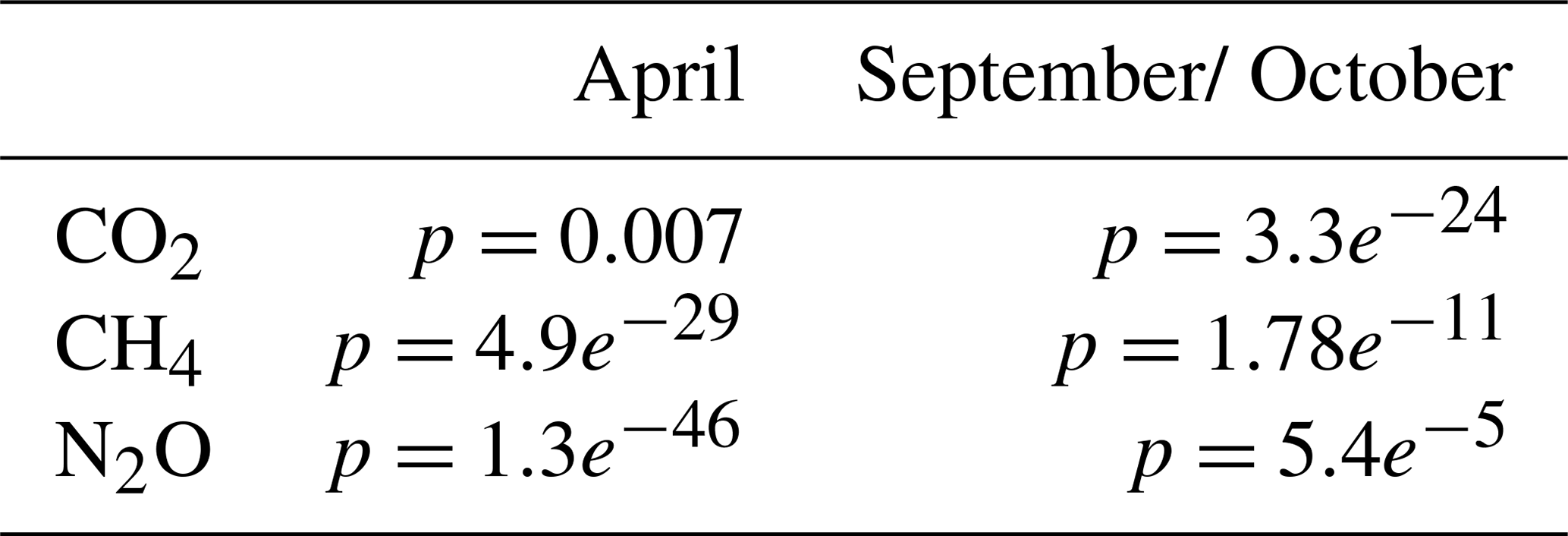
Table A2 Bonferroni-adjusted p-values from post hoc pairwise comparisons between bays; values less than 0.05 indicate statistically significant differences. No data is available for Östra Lermaren (ÖL) and Östra Myttingeviken (ÖM) in April. Furthermore, no N₂O data is available for Bodenviken (BV) in April.

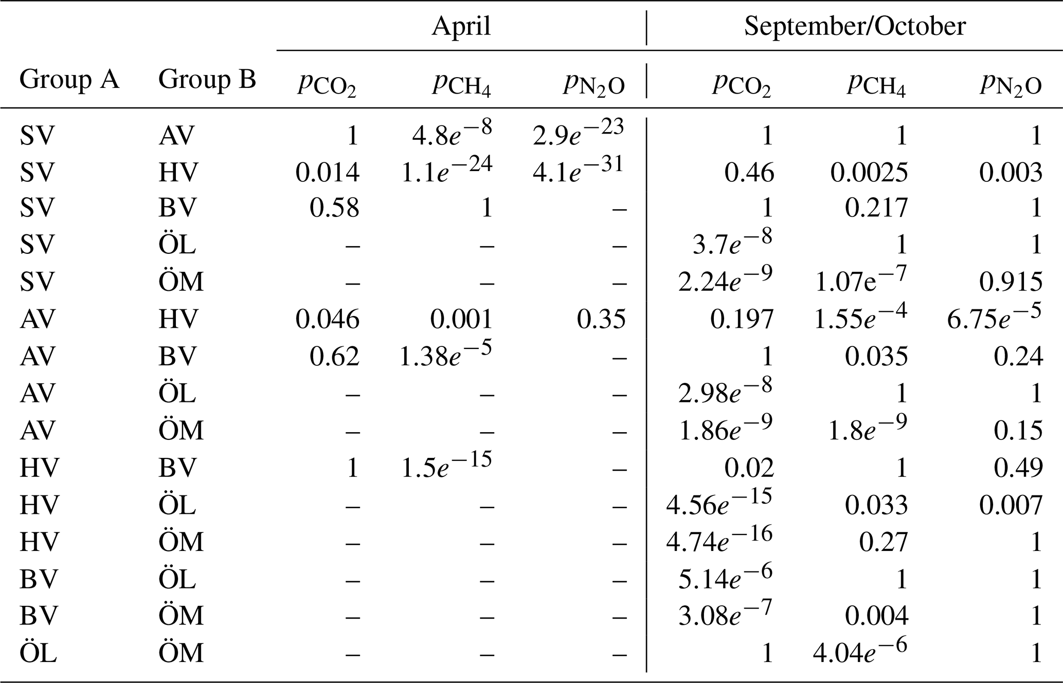
Table A3 A Wilcoxon ranksum test was conducted to test whether the concentrations of GHGs inside and outside the bays were significantly different. A difference is significant if h=1 and p<0.05. No data is available outside Östra Myttingeviken and no N₂O data is available for Bodviken (BV).

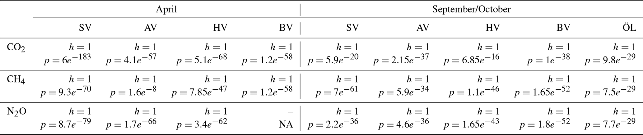
Table A4 Percentage contribution to the total net flux calculated as $\frac{\mathrm{abs}\left(\mathrm{mean}\right(F_{X,{\mathrm{CO}}_{\mathrm{2}}\mathrm{eq}}\left)\right)}{\mathrm{abs}\left(\mathrm{mean}\right(F_{{\mathrm{CO}}_{\mathrm{2}}}\left)\right)+\mathrm{abs}\left(\mathrm{mean}\right(F_{{\mathrm{CH}}_{\mathrm{4}},{\mathrm{CO}}_{\mathrm{2}}\mathrm{eq}}\left)\right)+\mathrm{abs}\left(\mathrm{mean}\right(F_{{\mathrm{N}}_{\mathrm{2}}\mathrm{O},{\mathrm{CO}}_{\mathrm{2}}\mathrm{eq}}\left)\right)}$. No N₂O data is available for Bodviken in April.

A2 Figures

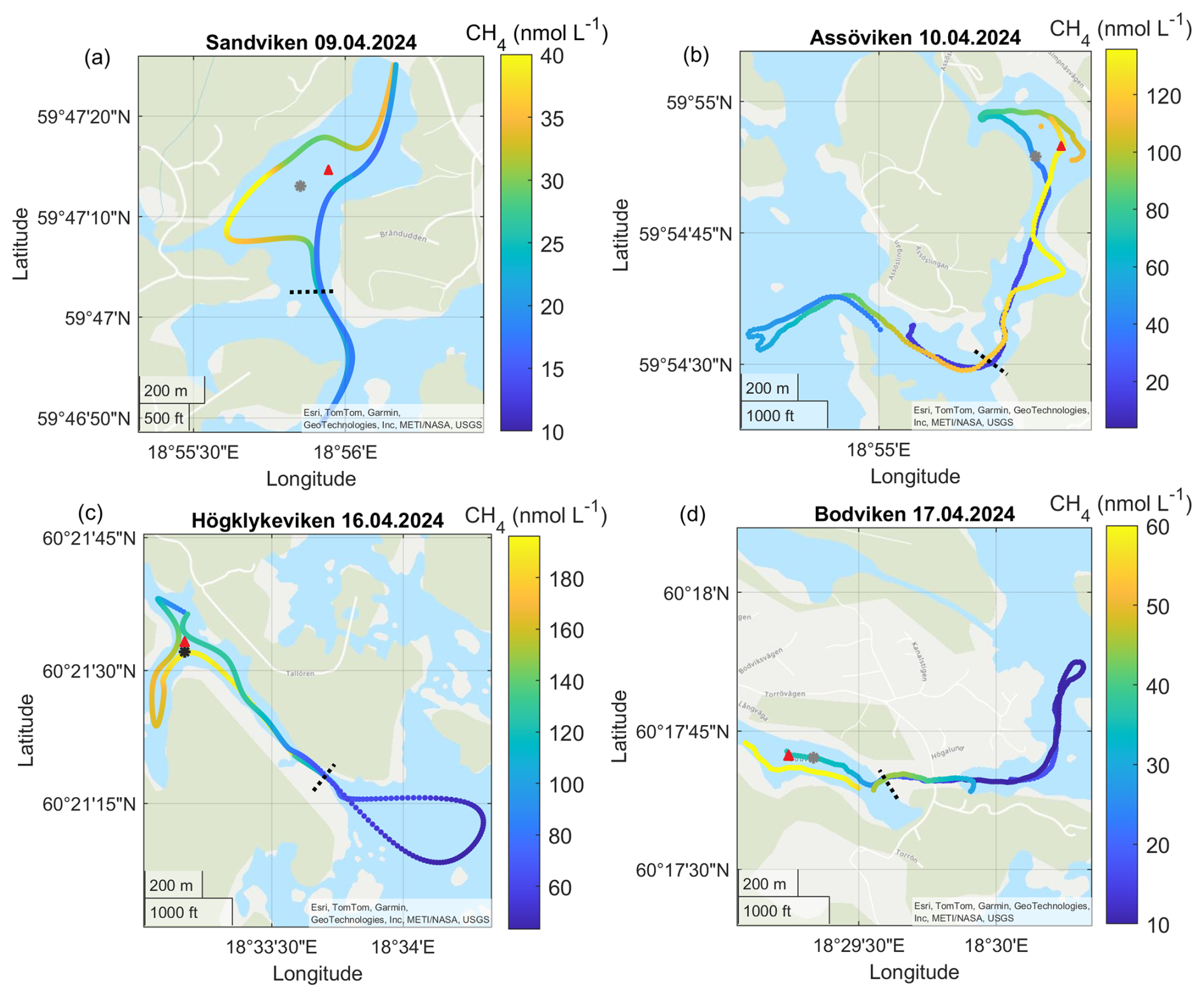
Figure A1 Surface water CH₄ concentrations in the different bays in April. Note the differences in scale between the different panels. The gray dots marks the sediment/water sampling locations during the GHG measurements, while red triangles mark long-term water monitoring stations. The dashed line marks the division between inside and outside bay area. Sources: Esri, TomTom, Garmin, GeoTechnologies, Inc, METI/NASA, USGS | Powered by Esri.

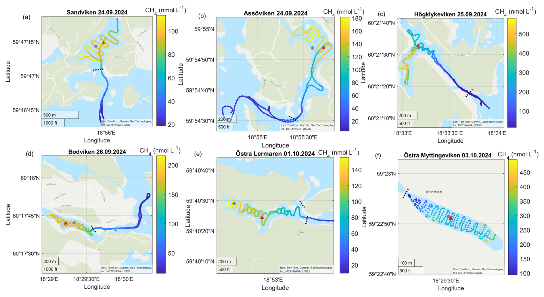
Figure A2 Surface water CH₄ concentrations in the different bays in September–October. Note the differences in scale between the different panels. The gray dots marks the sediment/water sampling locations during the GHG measurements, while red triangles mark long-term water monitoring stations. The dashed line marks the division between inside and outside bay area. Sources: Esri, TomTom, Garmin, GeoTechnologies, Inc, METI/NASA, USGS | Powered by Esri.

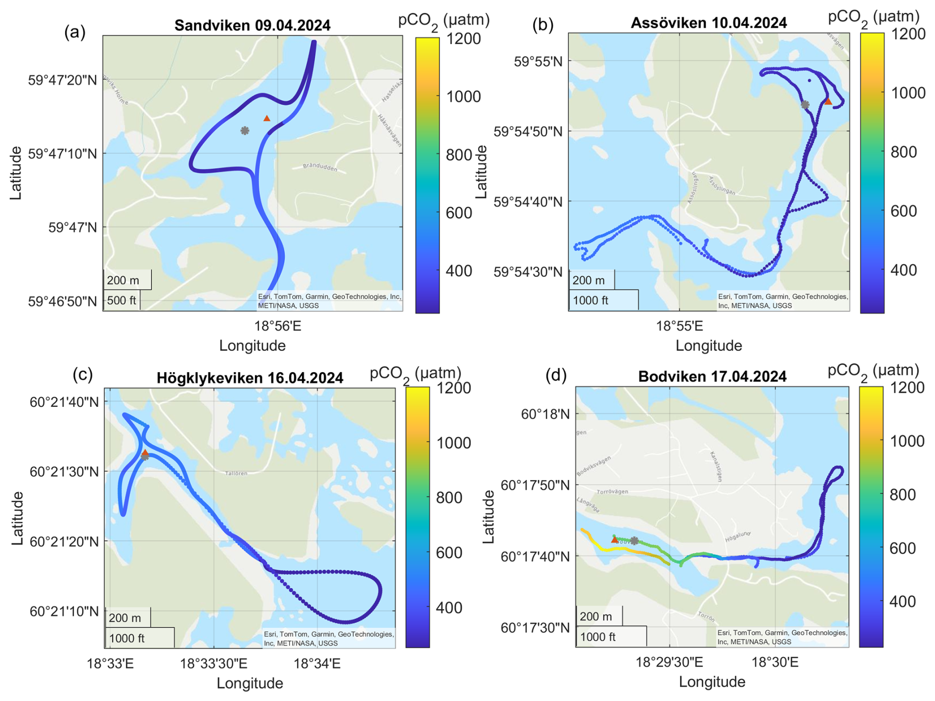
Figure A3 Surface water pCO₂ concentrations in the different bays in April. The gray dots marks the sediment/water sampling locations during the GHG measurements, while red triangles mark long-term water monitoring stations. The dashed line marks the division between inside and outside bay area. Sources: Esri, TomTom, Garmin, GeoTechnologies, Inc, METI/NASA, USGS | Powered by Esri.

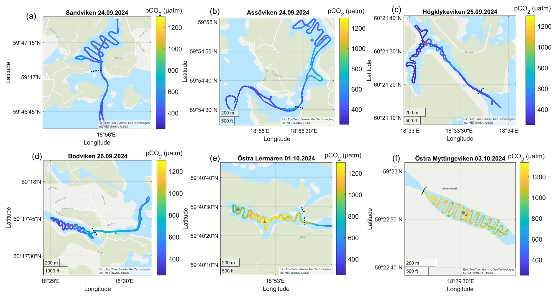
Figure A4 Surface water pCO₂ concentrations in the different bays in September–October. The gray dots marks the sediment/water sampling locations during the GHG measurements, while red triangles mark long-term water monitoring stations. The dashed line marks the division between inside and outside bay area. Sources: Esri, TomTom, Garmin, GeoTechnologies, Inc, METI/NASA, USGS | Powered by Esri.

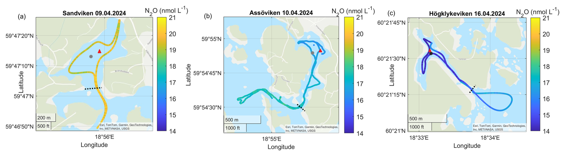
Figure A5 Surface water N₂O concentrations in the different bays in April. No N₂O data is available for Bodviken. The gray dots marks the sediment/water sampling locations during the GHG measurements, while red triangles mark long-term water monitoring stations. The dashed line marks the division between inside and outside bay area. Sources: Esri, TomTom, Garmin, GeoTechnologies, Inc, METI/NASA, USGS | Powered by Esri.

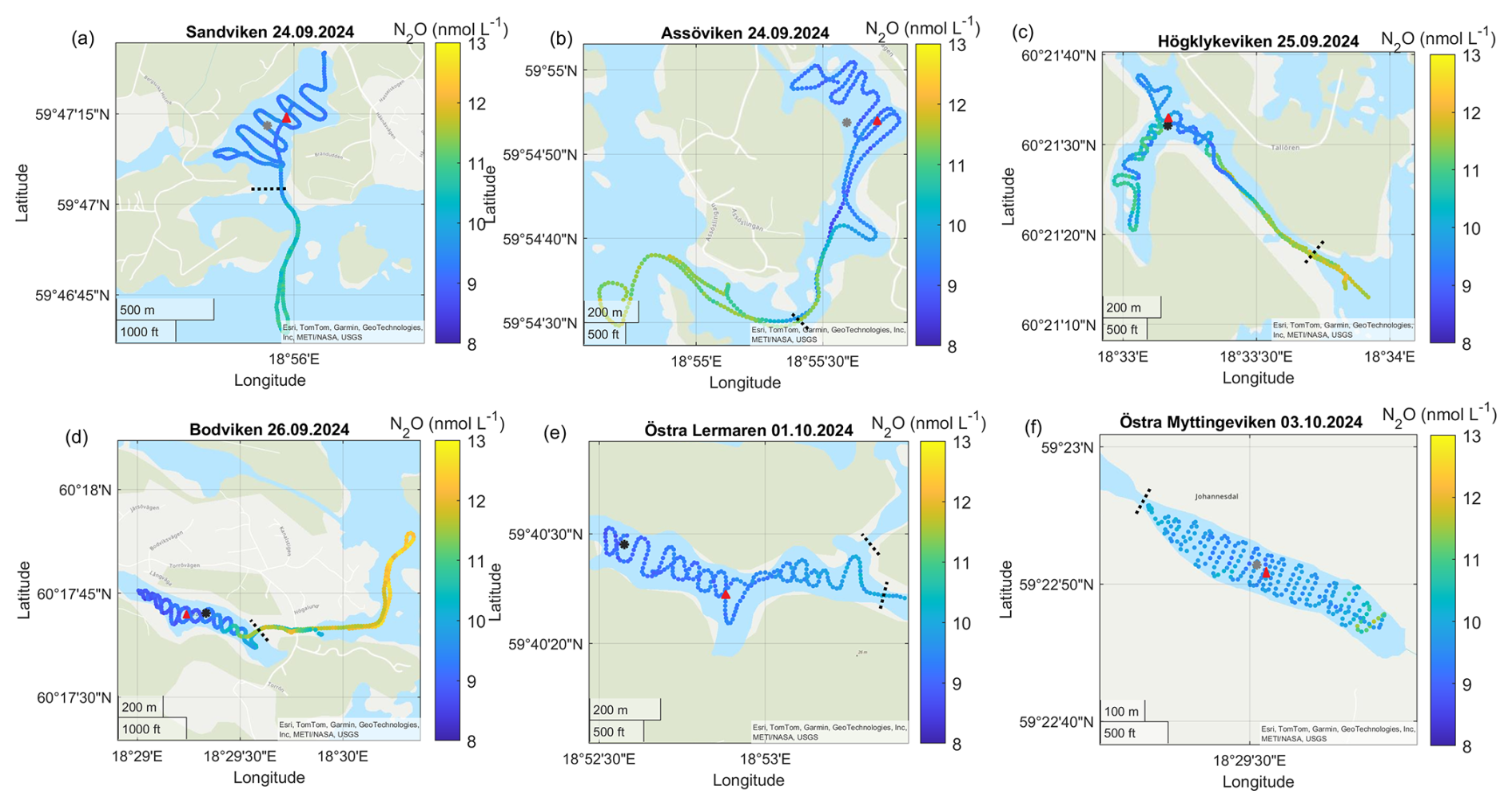
Figure A6 Surface water N₂O concentrations in the different bays in September–October. The gray dots marks the sediment/water sampling locations during the GHG measurements, while red triangles mark long-term water monitoring stations. The dashed line marks the division between inside and outside bay area. Sources: Esri, TomTom, Garmin, GeoTechnologies, Inc, METI/NASA, USGS | Powered by Esri.

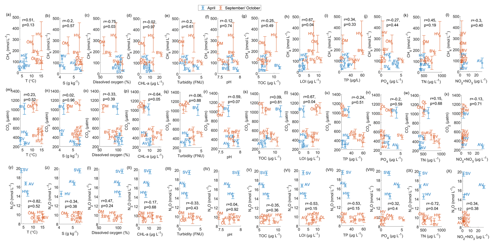
Figure A7 Relationships between seawater properties and GHG concentrations. Correlation coefficient and significance level are given for the combined data from April and September/October.

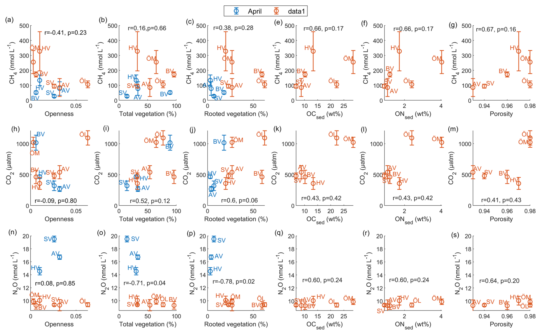
Figure A8 Relationships between bay characteristics (openness, vegetation cover and sediment properties) and GHG concentrations. Correlation coefficient and significance level are given for the combined data from April and September/October.