Understanding the balance between methane production and oxidation from wetlands: insights from a reduced process-based model

Wetlands play a crucial role in the global carbon cycle, both by sequestering large amounts of carbon in their soils and acting as a major natural source of atmospheric methane. Methane emissions depend strongly on soil temperature, substrate availability, and the depth of the water table relative to the soil surface, reflecting a balance between production, oxidation, and transport. Here we develop a simple mathematical model that captures how production and oxidation interact to control emissions. We condense these processes into a single ordinary differential equation, parameterised by water-table depth, soil temperature, and vegetation-derived carbon inputs, to mechanistically explore how these factors interact to control wetland methane emissions. Using emission data from six mid-latitude wetlands in the Prairie Pothole Region, we show that the model can reproduce seasonal and inter-annual variation in fluxes. Having established this agreement, we employ the model to investigate the conditions under which emissions are maximised. Peak fluxes consistently occur when the water table is at or just above the soil surface and are strongly modulated by wetland-specific parameters, with oxidation acting as a significant sink in some systems. Importantly, we find that the temperature sensitivity of oxidation is a key determinant of both the magnitude and location of peak emissions. These results highlight how warming may shift emission dynamics, emphasising the need for site-specific and adaptive wetland management and restoration strategies.

1 Introduction

Wetlands are soil-water ecosystems in which the persistent or recurring presence of water at or near the land surface strongly influences physical, chemical, and biological processes (Bansal et al., 2023a; Mitsch and Gosselink, 2015). Spanning a wide range of water depths and hydroperiods, wetlands occur in many forms, including marshes, swamps, bogs, fens, floodplain wetlands, tidal wetlands, and small, geographically isolated systems. Individual wetlands can range in size from well under 1 ha, as is typical for wetlands of the Prairie Pothole Region (PPR) of North America (Goldhaber et al., 2014), to expansive complexes covering hundreds or even thousands of square kilometres (Junk, 2024). Serving as a boundary between land and aquatic environments, these diverse and dynamic ecosystems provide a habitat for a variety of plants, animals, and microbes whilst also performing critical ecological functions such as water filtration, retention, and purification (Bridgham et al., 2006; Gleason et al., 2011; Zedler and Kercher, 2005). Given this wide array of functions, wetlands are often touted as a possible nature based solution (e.g. for flood prevention Ferreira et al., 2023) and there has been a recent push for their enhanced conservation given their previous loss due to anthropogenic activities, including widespread drainage, land conversion, and hydrological alteration associated with urbanisation and agricultural intensification (Bradford, 2016; Evenson et al., 2018; Fluet-Chouinard et al., 2023; Verhoeven and Setter, 2010).

Wetlands also play a significant role in the global carbon and nitrogen cycles, sequestering substantial amounts of carbon in their soils and storing roughly one-third of global soil carbon despite covering only 5 %–8 % of the land surface (Mitsch et al., 2013). Through active microbial processes, wetlands can both emit and uptake greenhouse gases (GHGs), including carbon dioxide (CO₂), nitrous oxide (N₂O), and methane (CH₄) (Bridgham et al., 2006; Salimi et al., 2021). In this study, we focus specifically on CH₄ dynamics, examining the balance between CH₄ production, oxidation, and emission from wetlands. Indeed, wetlands, together with inland waters, are responsible for approximately 83 % of natural global CH₄ emissions and 22 %–48 % of total CH₄ emissions (Forbrich et al., 2024; Saunois et al., 2019), with those located in tropical and mid-latitudes contributing significantly to the increase in global CH₄ concentrations in recent decades (Forbrich et al., 2024). Given the need to balance the local ecological benefits of wetlands against the global risks of enhanced GHG emissions and their contribution to climate change, improved understanding of emission mechanisms and more accurate estimates of total wetland emissions are required.

Emissions from individual wetlands are shaped by complex interactions between ecological, hydrological, climatic, and human influences. Among these, the position of the water table relative to the soil surface, soil temperature, and the supply of carbon substrates for CH₄ production exert the strongest controls (Moore and Dalva, 1993; Turetsky et al., 2014). These three drivers govern the balance of wetland CH₄ dynamics – methanogenesis (CH₄ production), methanotrophy (CH₄ oxidation), and release to the atmosphere via diffusion, ebullition, or plant-mediated transport. Field measurements of CH₄ fluxes, whether obtained from chamber studies or eddy-covariance systems, therefore capture the net outcome of these competing processes.

In wetland ecosystems, submerged soils provide the anaerobic conditions that favour methanogenesis (Hondula et al., 2021), where alternative electron acceptors are scarce and organic carbon decomposition proceeds slowly (Thauer and Shima, 2008). When the water table drops below the surface, methanogenesis is suppressed and CH₄ oxidation intensifies (Bansal et al., 2016); continued lowering exposes soil carbon pools to fully aerobic conditions, where microbes instead release CO₂ through respiration (Le Mer and Roger, 2001; Wu et al., 2024). Hence, water table position marks a demarcation between anaerobic production and aerobic consumption of CH₄ (Segers, 1998). Temperature further modulates both methanogenesis and oxidation through its control of microbial kinetics, accelerating reaction rates with warming, and dampening them when soils cool (Bansal et al., 2016). Meanwhile, vegetation biomass influences all stages of the CH₄ dynamics by supplying carbon substrate through the decomposition of organic matter, transporting oxygen to root zones that enhance local oxidation, and providing conduits for plant-mediated CH₄ emission in addition to diffusion and ebullition pathways (Bansal et al., 2020; Schütz et al., 1991; Stewart et al., 2024). These controls are strongly coupled. For example, soil water balance is governed by ecohydrologic processes such as infiltration, runoff, and evapotranspiration (Cui et al., 2024; Mitsch and Gosselink, 2015), which in turn are influenced by atmospheric and soil temperature as well as vegetation.

A wide range of models have been developed to quantify wetland CH₄ dynamics. At large scales, empirical or data-driven approaches are commonly used and often achieve high predictive accuracy (e.g. Bansal et al., 2023b; McNicol et al., 2023; Ying et al., 2024; Yuan et al., 2022). However, because these approaches link environmental drivers (e.g. water table, temperature, vegetation) directly to net emissions, they cannot distinguish the relative contributions of production, oxidation, and emission pathways. Moreover, data-driven models provide only limited mechanistic insight, making it difficult to interpret how or why fluxes respond to changing conditions. In contrast, process-based biogeochemical models such as DNDC (Li, 2000; Zhang et al., 2002; Haas et al., 2013) and ecosys (Grant and Roulet, 2002) provide accurate mechanistic descriptions for simulating nitrogen and carbon cycling in soils to predict N₂O, CO₂, and CH₄ fluxes. Other models, including the LPJ model (Smith et al., 2001; Wania et al., 2010), focus on the influence of wetland vegetation patterns on emissions, whilst WETMETH (Nzotungicimpaye et al., 2021) specifically addresses the dependence of emissions on soil moisture. Although they do so with varying degrees of sophistication, these models generally incorporate explicit representations of soil microbial processes (e.g. nitrification, denitrification, fermentation), plant growth and decay (e.g. photosynthesis and litter input), soil properties and hydrology, and carbon-nutrient interactions (for further details see reviews by Forbrich et al., 2024; Melton et al., 2013; Xu et al., 2016). However, despite their sophistication and predictive skill, they are often computationally intensive, require extensive parameterisation, and can make it difficult to isolate the mechanisms most responsible for observed CH₄ fluxes.

To improve interpretability and enable sensitivity analyses, simplified mechanistic models have been developed that focus on the dominant processes driving CH₄ fluxes, often using reduced reaction-diffusion-advection formulations combined with empirical parameterisations (e.g. Arah and Stephen, 1998; Walter et al., 1996; Walter and Heimann, 2000; Tang et al., 2010). A key emergent behaviour from such models is the existence of a critical water depth at which emissions peak, reflecting the balance between production and oxidation. Using a zero-dimensional framework, Calabrese et al. (2021) found a robust peak near 50 cm inundation depth across multiple datasets and wetland types. In their formulation, fluxes from a soil column were determined by CH₄ generation, oxidative loss, and release through diffusion, ebullition, and plant-mediated transport. Whilst the model reproduced observed peaks under inundated conditions (Calabrese et al., 2021; Cui et al., 2024), it was parameterised with fixed water depths and excluded dynamic variation in temperature or substrate supply. As a result, it remains unclear whether the critical depth is universal or instead shifts with drivers such as soil temperature, vegetation biomass, or seasonal hydrological change.

To explore these questions, we develop a minimal mechanistic model linking water-table depth, soil temperature, and vegetation activity to CH₄ production, oxidation, and emission in wetland soils. The model adapts the framework of Calabrese et al. (2021) and consists of a single ordinary differential equation parameterised by these environmental drivers, validated against growing-season flux observations from mid-latitude wetlands in the PPR. Our objective is to capture the key drivers of emission seasonality, determine how they jointly control the magnitude of peak CH₄ fluxes, and how the balance between production and oxidation sets the water depth at which this peak occurs. By focusing on a single, interpretable equation that captures the dominant processes, we provide a simple yet robust framework for predicting wetland CH₄ emissions under variable hydrological and climatic conditions.

2 Mathematical model

We represent the wetland as a collection of vertical one-dimensional soil columns. Each column is defined over the vertical coordinate z in the domain $z_b\le z\le z_s$, where z=z_s denotes the soil surface and z=z_b the soil base (see Fig. 1a). The water table lies at z=z_w(t), which may rise above z_s under inundated conditions. Henceforth, we focus on soil columns at the centre of each wetland and neglect lateral exchanges with adjacent columns. All processes of interest are therefore resolved only in the vertical direction. This assumption is justified as chamber-based flux measurements inherently reflect local conditions, supporting a column-wise modelling approach focused on vertical processes. Our subsequent analysis concentrates on the vertical dynamics of a representative soil column located at the wetland centre.

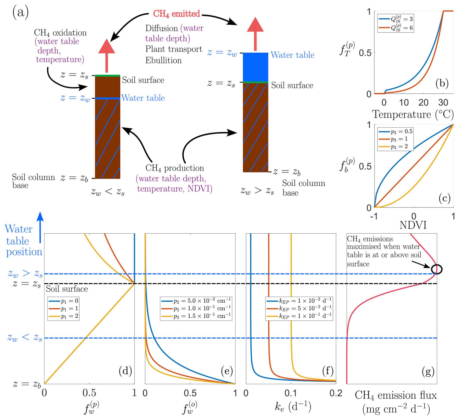
Figure 1 Conceptual model structure and environmental controls. (a) Schematic representation of two representative soil columns illustrating contrasting hydrological states: one with the water table below the soil surface (z_w<z_s) and one under inundated conditions (z_w>z_s). Purple annotations indicate the assumed environmental controls on CH₄ production, oxidation, and emission processes. Panels (b, c) show example functional dependencies used in the model: (b) dimensionless factor that describes temperature dependence of CH₄ production, $f_T^{\left(p\right)}$, and (c) dimensionless factor that describes NDVI dependence of CH₄ production, $f_b^{\left(p\right)}$, for different parameter choices. Panels (d, f) illustrate dependence on water table position relative to the soil surface: (d) $f_w^{\left(p\right)}$, the CH₄ production rate modifier; (e) $f_w^{\left(o\right)}$, the CH₄ oxidation rate modifier; and (f) k_e, the CH₄ emission rate, with two regimes highlighted (z_w<z_s and z_w>z_s), these simulations are run for z_s=0 cm and $z_b=-\mathrm{100}$ cm. Panel (g) presents a schematic of the resulting non-linear dependence of CH₄ emission flux on water table depth.

2.1 Model overview

We employ a simple ODE model to describe CH₄ emission from the soil column, accounting for the competing influence of methanogenesis and methanotrophy. We denote by M_s (mg CH₄ cm⁻²) the total mass of CH₄ in the soil column per unit ground area. Methane is produced in the soil column at rate f_p ($\mathrm{mg}{\mathrm{CH}}_{\mathrm{4}}{\mathrm{cm}}^{-\mathrm{2}}{\mathrm{d}}^{-\mathrm{1}}$), oxidised at rate f_o ($\mathrm{mg}{\mathrm{CH}}_{\mathrm{4}}{\mathrm{cm}}^{-\mathrm{2}}{\mathrm{d}}^{-\mathrm{1}}$), and emitted via plant transport, ebullition, and diffusion at rate f_e ($\mathrm{mg}{\mathrm{CH}}_{\mathrm{4}}{\mathrm{cm}}^{-\mathrm{2}}{\mathrm{d}}^{-\mathrm{1}}$). Hence, the CH₄ dynamics in soil can be summarised as

$$\begin{array}{}\text{(1)}& {\displaystyle \frac{\mathrm{d}{M}_s}{\mathrm{d}t}}=f_p-f_o-f_e,\end{array}$$

where the reaction and transport terms are parameterised by the water table depth, soil temperature and availability of carbon substrate due to plant biomass (in a similar manner to Gedney et al., 2004; Walter and Heimann, 2000). Figure 1 illustrates how CH₄ production, oxidation, and emission respond to these key environmental drivers.

2.2 Methane production

Wetland methanogenesis is governed by three primary environmental drivers: water table depth, soil temperature, and the availability of carbon substrate (Bridgham et al., 2013). Hence, we assume that the rate of CH₄ production in the soil column is given by

$$\begin{array}{}\text{(2)}& f_p=k_p{f}_T^{\left(p\right)}{f}_b^{\left(p\right)}{f}_w^{\left(p\right)},\end{array}$$

where k_p ($\mathrm{mg}{\mathrm{CH}}_{\mathrm{4}}{\mathrm{cm}}^{-\mathrm{2}}{\mathrm{d}}^{-\mathrm{1}}$) is a calibrated constant for each wetland, and the terms $f_T^{\left(p\right)}$, $f_b^{\left(p\right)}$, and $f_w^{\left(p\right)}$ are dimensionless scaling functions representing, respectively, the temperature dependence of methanogenesis (see Fig. 1b), the availability of carbon substrate due to plant biomass decay (see Fig. 1c), and the effect of water table depth on methanogenesis (see Fig. 1d).

Methanogenesis occurs in the anoxic layers of the soil and is therefore strongly dependent on water table depth. When the water table lies below the soil surface, higher water table depths increase the anoxic zone, promoting CH₄ production. However, waterlogged conditions can reduce CH₄ production if the available carbon substrate becomes distributed over an increasingly large water column above the soil surface, effectively reducing substrate availability for methanogenesis depending on the degree of mixing. As illustrated in Fig. 1d, we use the same piecewise water table dependence as Calabrese et al. (2021). In particular, we have

$$\begin{array}{}\text{(3)}& f_w^{\left(p\right)}=\left\{\begin{array}{ll}\left(\frac{z_w-z_b}{z_s-z_b}\right),& z_w<z_s\\ {\left(\frac{z_w-z_b}{z_s-z_b}\right)}^{-p_{\mathrm{1}}},& z_w\ge z_s\end{array}\right.,\end{array}$$

where $\mathrm{0}\le f_w^{\left(p\right)}\le \mathrm{1}$ (see Fig. 1d). The exponent p₁≥0 characterises CH₄ production in the region below the water table but above the soil column; p₁=0 corresponds to no mixing of carbon substrate, whereas p₁≫0 corresponds to well-mixed conditions. In other words, CH₄ production increases linearly with water table depth as the anoxic zone expands, such that $f_w^{\left(p\right)}=\mathrm{0}$ when the water table lies at the base of the soil column and $f_w^{\left(p\right)}=\mathrm{1}$ at the soil surface. Beyond the soil surface, further inundation reduces production, following a negative power-law relationship with $f_w^{\left(p\right)}\to \mathrm{0}$ as z_w→∞. Note that, whilst methanogenesis predominantly occurs in anoxic soil layers, small amounts of CH₄ may also be produced in oxic layers via micro-anoxic microsites within the soil column (Angle et al., 2017). These contributions are not explicitly resolved in our model, which focuses on bulk soil CH₄ production as the dominant source.

Three methanogenic pathways contribute to CH₄ production in wetlands: hydrogenotrophic, whereby bacteria reduce CO₂ with hydrogen to form CH₄; acetoclastic, in which bacteria convert acetic acid from decomposing organic matter into both CH₄ and CO₂; and methylotrophic methanogenesis, in which specialised methanogens convert methylated compounds (e.g. methanol, methylamines, or methyl sulphides) into CH₄, and may be particularly important in PPR wetlands (Conrad, 1999; Bechtold et al., 2025; Dalcin Martins et al., 2017; Thauer et al., 2008). Biomass availability thus plays a crucial role in all three pathways: directly through litter input for acetoclastic methanogenesis, indirectly via CO₂ production for hydrogenotrophic methanogenesis, and by supplying methylated compounds for methylotrophic methanogenesis. Despite differences in substrates and microbial mechanisms, we combine these pathways into a single effective methanogenesis term for model simplicity. To represent this dependence, we use the Normalised Difference Vegetation Index (NDVI) as a proxy for available plant biomass. NDVI, which ranges from −1 to 1, quantifies vegetation density and health based on the differential reflectance between near-infrared and red light, typically derived from satellite data. To account for the lag between vegetation growth and availability of decomposable organic matter, we introduce a delay τ days between NDVI and biomass availability (see Bansal et al., 2023b), such that

$$\begin{array}{}\text{(4)}& f_b^{\left(p\right)}={\left({\displaystyle \frac{\mathrm{1}+\text{NDVI}(t-\mathit{\tau })}{\mathrm{2}}}\right)}^{p_{\mathrm{3}}},\end{array}$$

where p₃≥0 (see Fig. 1c). This functional form ensures that $\mathrm{0}\le f_b^{\left(p\right)}\le \mathrm{1}$.

Soil temperature strongly regulates both major CH₄ production pathways through temperature-dependent enzyme kinetics (Yvon-Durocher et al., 2014). This influence is two-fold: higher temperatures enhance fermentation processes such as increased root exudation, and directly stimulate methanogen activity. The temperature dependence of methanogenesis typically follows an Arrhenius-type (i.e. exponential) relationship (Dunfield et al., 1993). Following previous models (e.g. Souza et al., 2021; Walter and Heimann, 2000), we represent this effect using a Q₁₀ formulation:

$$\begin{array}{}\text{(5)}& f_T^{\left(p\right)}=\left\{\begin{array}{ll}\mathrm{0},& T\le \mathrm{0}\mathrm{°}\mathrm{C}\\ Q_p^{\frac{\mathrm{1}}{\mathrm{10}}(T-\mathrm{30})},& \mathrm{0}\mathrm{°}\mathrm{C}<T<\mathrm{30}\mathrm{°}\mathrm{C}\\ \mathrm{1},& T\ge \mathrm{30}\mathrm{°}\mathrm{C}\end{array}\right.,\end{array}$$

where T (°C) is the soil temperature, Q_p≥1 is a fitted parameter, and $\mathrm{0}\le f_T^{\left(p\right)}\le \mathrm{1}$ (see Fig. 1b). This form reflects enzymatic saturation above an optimal temperature, which we set at 30 °C due to the mid-latitude wetland focus, where temperatures rarely exceed this threshold. Under future climate scenarios with more frequent extreme heat, CH₄ production may continue to increase above 30 °C, in which case our current formulation would be conservative. Alternatively, enzymatic and microbial activity may decline above their thermal optimum due to heat stress, potentially suppressing production. The net effect will likely vary among wetlands with different thermal regimes and microbial communities, and warrants further modelling investigation.

2.3 Methane oxidation

Methane produced in the soil column may be oxidised before reaching the surface, thereby preventing its emission into the atmosphere. This oxidation occurs predominantly under aerobic conditions in the unsaturated soil zone and is therefore strongly modulated by the position of the water table. Additionally, soil temperature regulates the activity of methanotrophic bacteria (Segers, 1998).

We refine the model of Calabrese et al. (2021) by assuming that CH₄ oxidation follows first-order reaction kinetics that depend on water-table depth (cf. CH₄ production, which is treated as a zero-order process, reflecting that methanogenesis is primarily controlled by substrate availability rather than the instantaneous CH₄ concentration within the soil column). In our formulation, oxidation is further modified by temperature through a multiplicative factor, such that

$$\begin{array}{}\text{(6)}& f_o=k_o{f}_T^{\left(o\right)}{f}_w^{\left(o\right)}{M}_s,\end{array}$$

where k_o (d⁻¹) is the maximum oxidation rate under atmospheric oxygen availability throughout the soil column; $f_T^{\left(o\right)}$ and $f_w^{\left(o\right)}$ are dimensionless functions describing the dependence of methanotrophy on soil temperature and water table depth, respectively. For simplicity, oxygen transport via plant roots, which could enhance methanotrophy, is neglected here. Moreover, our model assumes that CH₄ oxidation occurs predominantly under aerobic conditions in the unsaturated soil zone. Anaerobic oxidation of CH₄ in saturated layers, which requires alternative electron acceptors (e.g. sulphate or nitrate, see Segarra et al., 2015), is not explicitly resolved and may slightly reduce net CH₄ flux in some wetlands.

In the current model, we only resolve aerobic oxidation and neglect these secondary anaerobic pathways for simplicity. Following Calabrese et al. (2021), we model the water table dependence of oxidation as an exponential decay with increasing water table depth:

$$\begin{array}{}\text{(7)}& f_w^{\left(o\right)}={\mathrm{e}}^{-p_{\mathrm{2}}(z_w-z_b)},\end{array}$$

where p₂>0 (cm⁻¹) is a control parameter (see Fig. 1e). Thus, oxidation is maximal when the water table is at the base of the soil column (z_w=z_b) and decreases sharply as the water table rises. To capture temperature dependence, we employ a Q₁₀ relationship analogous to that used for CH₄ production (e.g. Walter and Heimann, 2000):

$$\begin{array}{}\text{(8)}& f_T^{\left(o\right)}=\left\{\begin{array}{ll}\mathrm{0},& T\le \mathrm{0}\mathrm{°}\mathrm{C}\\ Q_o^{\frac{\mathrm{1}}{\mathrm{10}}(T-\mathrm{30})},& \mathrm{0}\mathrm{°}\mathrm{C}<T<\mathrm{30}\mathrm{°}\mathrm{C}\\ \mathrm{1},& T\ge \mathrm{30}\mathrm{°}\mathrm{C}\end{array}\right.,\end{array}$$

where Q_o≥1 is a constant.

2.4 Methane emissions

Methane produced in the soil column is emitted into the atmosphere by three distinct mechanisms: diffusion, plant transport, and ebullition. We assume emission by diffusion occurs at rate k_D (d⁻¹), emission due to plant transport at rate k_PT (d⁻¹), and emission due to ebullition at rate k_EB (d⁻¹). We employ a simple functional form (see Fig. 1f) for CH₄ emission:

$$\begin{array}{}\text{(9)}& f_e=k_e{M}_s,k_e=k_D+k_{EB}+k_{PT}.\end{array}$$

Emission is treated as first-order, dependent on the total soil CH₄ pool. Such a simple form neglects the vertical motion of CH₄ (e.g. detailed in models by Walter et al., 1996; Zhang et al., 2002) but has been demonstrated to successfully describe key aspects of CH₄ emission (Calabrese et al., 2021).

Diffusive release involves CH₄ movement down gradients from regions of high CH₄ concentration in the anaerobic soil to the atmosphere. This transport is slow and subject to methanotrophic oxidation, but typically dominates when soils are moist or water columns are deep and oxygenated. The effectiveness of diffusion decreases with water table depth, since the diffusive path lengthens and so the rate of diffusive release scales inversely. Hence, the rate of diffusive transport of CH₄ is given by

$$\begin{array}{}\text{(10)}& k_D={\displaystyle \frac{D}{{\left(z_w-z_b\right)}^{p_{\mathrm{4}}}}},\end{array}$$

where D is the diffusion coefficient of CH₄ and p₄=2 for Fickian diffusion. Soil temperature can provide an additional layer of complexity, by affecting water viscosity and gas diffusion, though we neglect this.

Meanwhile, plant transport and ebullition provide more efficient emission routes. In the case of plant transport, CH₄ travels along gas conduits (e.g. roots, stems) in aerenchymous plants or tree stems by means of convective flow, molecular diffusion, or pressure-driven transport (Joabsson et al., 1999). This allows CH₄ to bypass much of the (aerobic) oxidation zone, preventing methanotrophy (Laanbroek, 2010). The effectiveness of this bypass increases with higher water tables, particularly when z_w>z_s, as plant-mediated transport can transport CH₄ directly from saturated soil to the atmosphere, thereby avoiding oxidation in near-surface oxic zones (Bansal et al., 2020). On the other hand, ebullition provides a sporadic emission mechanism due to bubbling of supersaturated CH₄. These emission pulses bypass methanotrophy almost entirely and are triggered when gas pressure overcomes surface tension, typically in response to fluctuations in hydrostatic or atmospheric pressure, or changes in temperature (Baron et al., 2022; Walter et al., 2006). We assume, in an identical manner to Calabrese et al. (2021), that plant transport and ebullition occur at a constant rate, which for the remainder of this paper we couple into one term, $k_{EP}=k_{EB}+k_{PT}$. However, future model refinements could link plant transport to NDVI and water table depth, and ebullition to changes in weather conditions and water table depth.

2.5 Computational method

We solve the single ODE (Eq. 1) in Matlab using the inbuilt stiff solver ode15s and employ default error tolerances. The results are well converged, even for long simulation times. Model parameters are calibrated to individual wetlands by minimising the normalised root mean square error (nRMSE) between observed (oF_i) and predicted (pF_i) CH₄ flux at each data point $i=\mathrm{1},\mathrm{2},\mathrm{\dots },N$, defined as

$$\begin{array}{}\text{(11)}& \begin{array}{rl}{\displaystyle }\text{nRMSE}& {\displaystyle }=\text{RMSE}/\mathit{\sigma },\\ {\displaystyle }\text{RMSE}& {\displaystyle }=\sqrt{{\displaystyle \frac{{\sum }_{i=\mathrm{1}}^N{\left(p{F}_i-o{F}_i\right)}^{\mathrm{2}}}{N}}},\end{array}\end{array}$$

where σ is the standard deviation of observed fluxes. This normalisation facilitates comparison of model performance across wetlands with differing flux magnitudes (Wania et al., 2010).

To identify the set of optimised parameters for a particular wetland, we use the inbuilt Matlab genetic algorithm (ga), a population-based, stochastic global optimisation method. This algorithm is particularly suited for solving non-linear and discontinuous optimisation problems where gradient-based methods struggle to converge or become trapped in local minima. In particular, we minimise the nRMSE between model output and observations by calling ga, which searches the global parameter space until certain convergence criteria are met. Following Calabrese et al. (2021), the effective diffusivity of CH₄ in the soil is fixed at $D=\mathrm{1.3}{\mathrm{cm}}^{\mathrm{2}}{\mathrm{d}}^{-\mathrm{1}}$ in all simulations. All other parameters are adjusted during calibration and fitted individually for each wetland to capture site-specific environmental conditions. This approach allows the model to account for variation in soil properties, hydrology, and vegetation among wetlands, thereby reflecting wetland-specific biogeochemical and hydrological dynamics. The ranges of possible parameter values are detailed in Table A2.

3 A case study

To assess the ability of our model to capture both seasonal and inter-annual variability in CH₄ emissions, we calibrate model parameters using observational data from mid-latitude wetlands. These ecosystems are significant CH₄ sources and exhibit strong climatic variability, particularly in temperature and precipitation (Bridgham et al., 2013; Mushet et al., 2022; Renton et al., 2015). We concentrate on wetlands within the PPR of North America, a region which spans approximately 900 000 km² and encompasses portions of Alberta, Saskatchewan and Manitoba in Canada, and Montana, North and South Dakota, Minnesota, and Iowa in the United States (Mushet et al., 2022). This area is characterised by a large population of small, shallow, depressional wetlands formed during glacial retreat more than 10 000 years ago and exhibit highly seasonal hydrological microbial dynamics (Eisenlohr, 1972).

We focus on the Cottonwood Lake Study Area (CLSA) of the PPR, located in Stutsman County, North Dakota. The CLSA wetlands typically contain clay-rich soils, interspersed with pockets of sand and silt; the surrounding upland consists of hummocky hilltops and native grassland vegetation (Mushet et al., 2022). The 20 wetlands within the CLSA can be broadly classified based on their hydroperiod with 11 permanent (P1–P11) and 9 temporary (T1–T9) wetlands; wetlands P1–P9 and T1–T9 are shown in Fig. 2. Such a classification allows for the model to be tested across different wetland regimes that typically form different parts of the wetland continuum (Euliss et al., 2014). The permanent wetlands typically retain water year-round (except during severe drought). Most are closed basins, accumulating solutes over time, with only P3 and P8 regularly overflowing. Wetlands P2 and P7 appear hydraulically isolated, except for possible subsurface flows. These features, together with long water residence times and recharge from surrounding wetlands, mean many of these wetlands exhibit high sulphate concentration, suppressing methanogenesis via competitive sulphate reduction (Dalcin Martins et al., 2017). Larger surface-area-to-perimeter ratios in these wetlands may further reduce emissions. In contrast, the CLSA temporary wetlands typically dry out during the summer season and exhibit pronounced seasonal variability (Stewart and Kantrud, 1971). These wetlands (with the exception of T1 and T9) are open basins that overflow during high-water events, limiting the maximum water depth and promoting discharge to surrounding wetlands. Their repeating filling (by rainfall) and draining leads to fresher conditions and lower salinity, amplified by the low hydraulic conductivity characteristic of the PPR wetlands (Richardson et al., 1994). This wetland heterogeneity makes the CLSA an ideal testing site for our model performance.

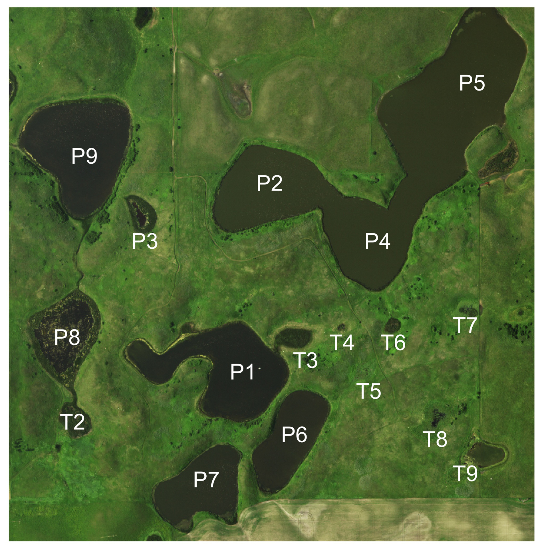
Figure 2 Cropped RGB satellite image centred on the CLSA (P10–P11 not shown). Image is derived from National Agriculture Imagery Program (NAIP) aerial imagery acquired on 20 July 2014, accessed via the USGS EarthExplorer platform (US Geological Survey, 2014). Image has been rescaled and spatially cropped for clarity. Source: NAIP, US Geological Survey (public domain).

3.1 Parameter ranges and fitting

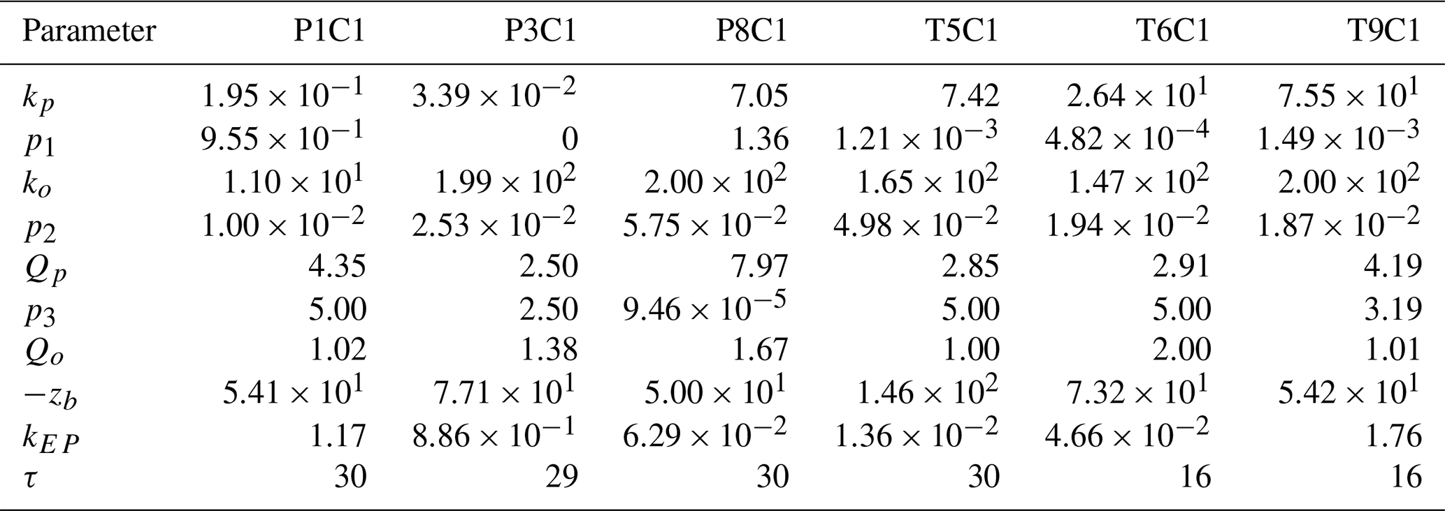
We fit model parameters for each wetland using the dataset provided by Bansal et al. (2023b), which includes data at approximately fortnightly (occasionally coarser) intervals for NDVI, soil temperature, water depth, water-filled pore space (WFPS) at the soil surface and CH₄ flux throughout the growing season (April–November). To reduce bias from extreme outliers in CH₄ flux measurements, likely caused by ebullition or anthropogenic disturbance, we exclude data points where CH₄ fluxes exceed 20 times the interquartile range for each wetland. The possible parameter ranges for each wetland are given in Table A2 in Appendix A, based on an extensive review of the literature. Given our focus on the wetland centre, we use flux measurements from a single chamber located near the centre of each wetland (Chamber 1 in the dataset). Measurements from other wetland or upland chambers are not included in the analysis.

When the water table lies above the soil surface, direct measurements of water depth are available. For periods when the water table falls below the surface, observed water depths are truncated at 0 cm, so subsurface positions must be estimated. For simplicity, to estimate z_w when the water table is below the surface, we assume a linear relationship with WFPS. Zero water depth measurements are replaced with these estimates and capped at $z_w=-\mathrm{49.9}\mathrm{cm}$ to remain within the model domain. This approach neglects lateral flow and potential time lags between water table changes and CH₄ emissions, but provides a first-order seasonal estimate adequate for budget calculations, which are usually dominated by periods when the water table is at or above the soil surface.

In order to force our model at the daily scale, we linearly interpolate between observations for all model drivers, i.e. NDVI, soil temperature, water depth and WFPS (a similar approach is employed by Walter and Heimann, 2000). We also introduce “ghost” data points two weeks before and after the observed growing season for each year, assuming T=0 °C and F=0 $\mathrm{mg}{\mathrm{CH}}_{\mathrm{4}}{\mathrm{cm}}^{-\mathrm{2}}{\mathrm{d}}^{-\mathrm{1}}$ (i.e. no CH₄ flux) to reflect dormancy in the winter, whilst holding NDVI and water table depth constant in this two week period. As discussed in Sect. 2, NDVI is introduced as a calibrated time-lagged forcing term, using values from τ days prior to account for the delay between photosynthetic activity and substrate availability due to plant growth and litter decomposition. Note that observed total CH₄ emissions are estimated by linearly interpolating daily flux measurements and numerically integrating them over each seasonal period.

Full details on the measurements used to force the model are provided by Bansal et al. (2023b), but we summarise briefly here. Methane fluxes were measured in the wetland zone of undrained PPR wetlands using static chambers deployed on sediment or floats along a single transect per wetland, with five wetland-zone sampling locations spaced from the edge to the centre. Measurements were collected approximately every two weeks during the growing season (May–November), between 10:00 and 14:00 LT, and included water depth, soil temperature (or water temperature when the water table exceeded 10 cm), air temperature, and soil volumetric water content (with WFPS calculated by dividing by soil porosity). NDVI corresponding to each sampling event was obtained from Landsat imagery to represent vegetation availability. These variables provide the spatially and temporally resolved forcing used in the chamber-scale model. As measurements are limited to the top 5–10 cm of soil (or water surface), daytime sampling, and relatively coarse NDVI (30 m), short-term heterogeneity may be smoothed or under-represented.

3.2 Summary of assumptions

For clarity, we briefly reiterate the key structural assumptions implicit in our model formulation. First, subsurface hydrology is represented through a simplified relationship between water-table depth and WFPS, implicitly assuming monotonic pore saturation with rising water tables and neglecting hysteresis, preferential flow paths, and fine-scale soil heterogeneity. Second, CH₄ production combines hydrogenotrophic, acetoclastic, and methylotrophic pathways into a single effective term rather than treating each microbial mechanism explicitly; small contributions from CH₄ production in oxic microsites are neglected. Third, CH₄ emission is treated as a first-order process, with diffusion represented explicitly and plant-mediated transport and ebullition combined into a single term, k_EP. In reality, ebullition is episodic and sensitive to temperature and pressure fluctuations, whilst plant-mediated transport depends strongly on vegetation phenology and water-table depth. This simplification neglects detailed vertical transport dynamics and the pulsed nature of ebullition, but is expected to primarily influence short-term emission variability rather than seasonal totals. Fourth, CH₄ oxidation is assumed to occur predominantly under aerobic conditions in the unsaturated soil zone, whilst anaerobic oxidation in saturated layers, which requires alternative electron acceptors (e.g. nitrate or sulphate), is not explicitly resolved. Fifth, the model resolves dynamics within a vertically homogeneous soil column at the wetland centre, neglecting lateral transport and edge effects; this assumption is likely less appropriate near the wetland boundary. Finally, to reduce bias from extreme CH₄ flux outliers (e.g. large ebullition events or disturbance), we exclude observations exceeding 20 times the interquartile range for each wetland, whilst retaining background ebullitive fluxes.

Together, these assumptions favour interpretability and parameter identifiability, capturing dominant seasonal controls on CH₄ flux whilst smoothing short-term variability and episodic pulses. They may, however, bias short-term fluxes under extreme hydrological conditions; for example, linear WFPS assumptions may overestimate production in partially saturated soils, pathway lumping smooths short-term variability, and neglecting oxygen transport may slightly overestimate net emissions. Near wetland edges, lateral flows, variable soils, and heterogeneous vegetation may further alter methane dynamics, meaning central-column assumptions likely break down within a few meters of the boundary.

4 Results

4.1 Model performance

To assess how well the model captures observed emission patterns, Figs. 3 and 4 show baseline simulations using optimised parameters derived using the method described in Sect. 2.5 (see Table A1 for details). In particular, Fig. 3 compares modelled CH₄ fluxes (blue line) with observations (red crosses) for the 2009–2016 growing seasons (note that Bansal et al., 2023b, provide data for wetland T5 only through 2015). The corresponding cumulative emissions are presented in Fig. 4, where predicted (blue) and observed (red) totals show close agreement. Panels (a)–(f) correspond to wetlands P1, P3, P8, T5, T6, and T9, respectively, spanning permanent and temporary types and representing a range of hydrological settings (Euliss et al., 2014): three recharge wetlands (P3, T5, T6), one discharge (P1), one flow-through (P8), and one apparently hydrologically isolated site (T9). The full response to modelled environmental drivers are detailed in Sect. S1 in the Supplement.

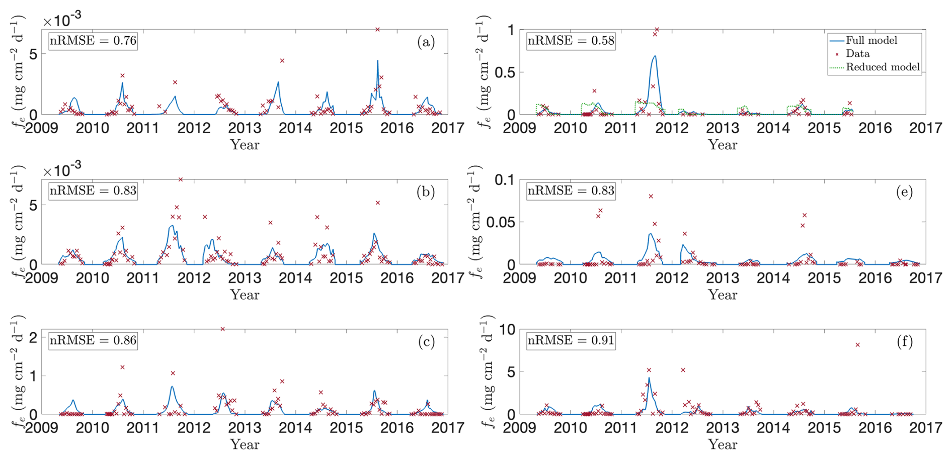
Figure 3 Model predictions versus observed CH₄ fluxes for selected wetlands in the CLSA. Panels show modelled (blue lines) and observed (red crosses; data from Bansal and Tangen, 2022) growing-season fluxes (2009–2016) for wetlands (a) P1, (b) P3, (c) P8, (d) T5, (e) T6, and (f) T9. These sites were chosen to represent the range of wetland types – permanent, temporary, source, sink, and flow-through. In panel (d), the green line shows predictions without temperature and NDVI dependence, corresponding to the framework of Calabrese et al. (2021).

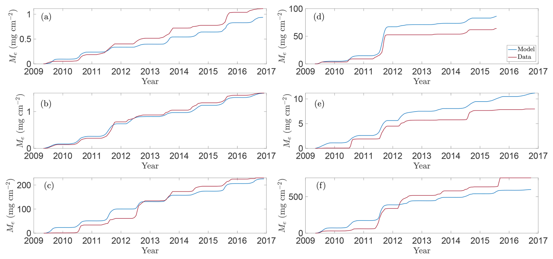
Figure 4 Model predictions versus approximate total observed CH₄ emissions for selected wetlands in the CLSA. Panels show modelled (blue line) and approximate observed (red line; based on data from Bansal and Tangen, 2022) total CH₄ emissions for wetland centres over the growing seasons 2009–2016 for wetlands (a) P1, (b) P3, (c) P8, (d) T5, (e) T6, and (f) T9.

The data reveal a clear positive correlation between CH₄ fluxes and both soil temperature and NDVI, which overall the model reproduces well. Emissions typically peak in mid- to late-growing season (July–September), when temperatures are highest and plant deterioration begins, demonstrating the importance of including these environmental drivers. The model captures the major flux dynamics, responding realistically to both soil temperature and vegetation activity, and also reproduces the near-zero CH₄ emissions observed in early spring and late autumn, when low temperature and limited substrate constrain methanogenesis. Meanwhile, the relationship between emissions and water-table depth is more complex (see Sect. 5.3 below). Variations in water level influence CH₄ production, oxidation, and transport not only directly, but also indirectly by changing factors such as wetland salinity or the concentration of alternative electron acceptors. These effects contribute to the significant heterogeneity in peak fluxes between wetlands. In particular, field observations indicate temporary wetlands generally exhibit higher emissions (Mushet et al., 2022).

Focusing first on the permanent wetlands, model performance is strong for wetland P1 (Fig. 3a), particularly during the 2009, 2010, 2015, and 2016 growing seasons. In 2015 the model captures two distinct seasonal emission peaks that align with observed soil-temperature maxima, reflecting its sensitivity to temperature forcing. Wetland P3 likewise demonstrates the need for the additional environmental drivers: during the 2010, 2011, and 2015 seasons, water depth remains nearly constant early in the year whilst emissions increase in tandem with lagged NDVI and temperature. Moreover, rare anomalously high CH₄ fluxes outside this window often coincide with elevated lagged NDVI or temperature, such as the early 2012 peak (Fig. 3b), driven by a large carbon substrate pool (see Fig. S1f in the Supplement). Performance for wetland P8 is more mixed. The model generally reproduces the overall pattern of low spring and autumn fluxes and higher summer emissions, together with the early 2012 peak, but performs poorly in 2009 and 2011. During both years emissions remain unexpectedly low despite favourable temperatures, water depths, and typical vegetation growth, leading the model to overestimate total seasonal fluxes (Fig. 4c). This discrepancy may reflect additional hydrological complexities: as a flow-through wetland, P8 may experience transient salinity or redox dynamics not represented in the model.

Overall, the model also performs well for the temporary wetlands, particularly for wetland T5 (Fig. 3d), where it correctly captures the trend in each season and reproduces the pronounced peak in CH₄ emissions during the 2011 growing season (in response to elevated soil temperatures, see Fig. S4e in the Supplement). Moreover, the model replicates muted emissions in 2012, when the water table remained below the soil surface (Fig. S4d). This clearly demonstrates the modulating influence of water table depth; for example, unlike in wetland P3, emissions in T5 do not appreciably rise early in 2012 despite anomalously early plant growth (Fig. S4f). Results are more mixed for wetland T6 (Fig. 3e) but relatively strong for wetland T9 (Fig. 3f). In 2012 both wetlands also experienced unusually early plant growth; in T6, the model correctly captures the peak emissions in April–May, followed by a decline. In both T6 and T9, the model captures the high summer 2011 fluxes, driven by elevated soil temperatures (Figs. S5e and S6e in the Supplement). Meanwhile, for T9 the model reproduces negligible 2016 emissions, attributable to low water table, cooler soil, and limited substrate, but it misses a sharp late-season spike in 2015. Excluding this outlier substantially reduces the nRMSE, making T9 one of the best-described sites overall. The 2015 spike coincides with a rapid water-table drop and is likely due to ebullition or enhanced diffusion, suggesting the need for more detailed representation of these processes in future model iterations.

In Fig. 3d we also compare our full model with the reduced Calabrese et al. (2021) formulation, demonstrating the benefit of including vegetation and temperature drivers. Focusing on wetland T5, the framework of Calabrese et al. (2021) capably describes steady-state behaviour, but fails to reproduce the strong seasonal variability in CH₄ fluxes. Incorporating a Q₁₀ temperature dependence for methanogenesis and oxidation substantially improves the timing and magnitude of predicted emissions, highlighting the dominant role of temperature under inundated conditions. Yet temperature alone cannot explain all observed fluctuations. Including NDVI as an independent proxy for substrate availability is crucial, particularly in reproducing anomalous early-season peaks such as those in various wetlands in 2012. Given the central roles of temperature and substrate availability, we also tested whether including water-table depth improves model performance (results not shown). For permanent wetlands, which typically remained inundated, the effect is minor, consistent with the optimised parameters in Table A1 that indicate a weak exponential decay of oxidation and a near-zero depth dependence of methanogenesis. In contrast, the influence of water-table depth is much stronger in temporary wetlands, where CH₄ emissions drop sharply once the water table falls below the soil surface.

We further assess model performance in Fig. 5, which also compares predicted and observed CH₄ emissions for each wetland during the 2009–2016 growing seasons (using the same optimised parameters detailed in Table A1). In particular, we present a scatter plot comparing total seasonal emissions in each wetland, perfect model agreement would place data points on the 1:1 grey reference line (i.e. the predicted and observed emissions are equal). At the daily scale, model performance is generally reasonable but shows a consistent bias toward overestimating low emissions, a pattern most evident in temporary wetlands where the water table frequently drops below the surface. However, because these low-flux periods contribute little to the seasonal CH₄ budget (except for brief spikes as the water table falls), integrated emissions remain generally well captured. Indeed, seasonal totals are reproduced reasonably for both permanent and temporary wetlands, including high-emission years such as T9 in 2011, though the model occasionally underestimates emissions when large, infrequent flux events occur and overestimates in years with persistently low observed fluxes (Fig. 5). Performance is notably stronger in permanent wetlands, where water levels typically remain above the surface and fluxes are more stable.

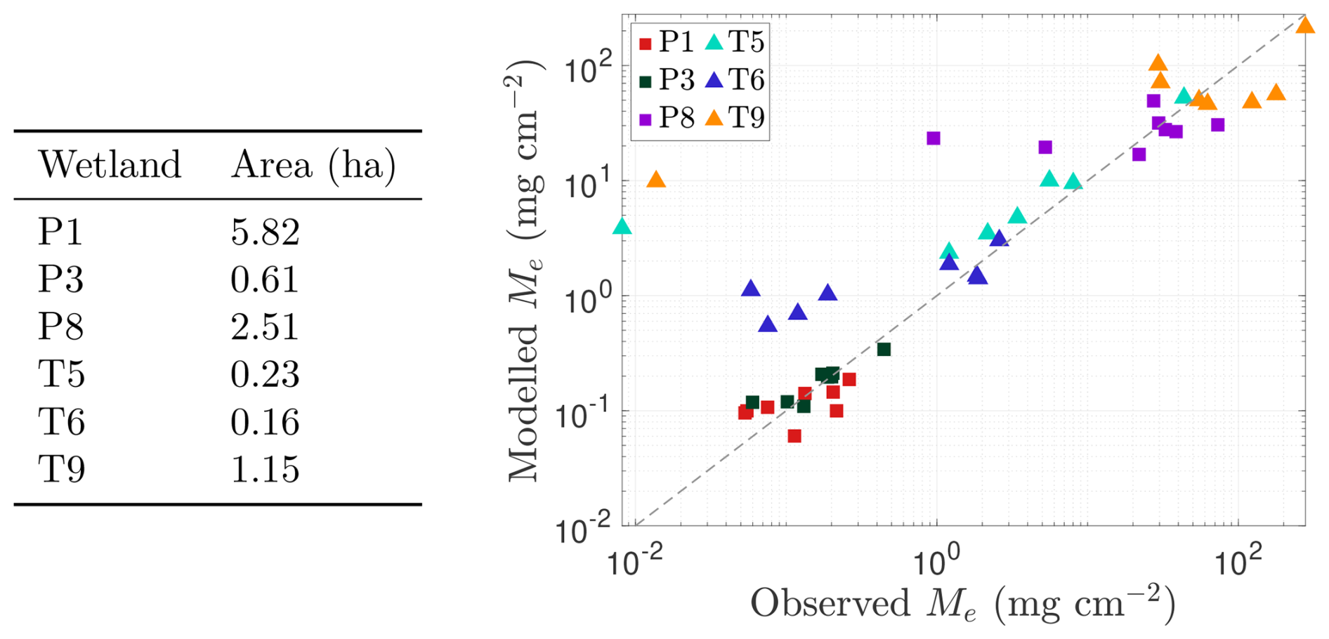
Figure 5 Assessment of model performance in capturing methane (CH₄) emissions from each wetland (P1, P3, P6, P8, T5, T6, and T9) during the 2009–2016 growing seasons. Scatter plot of approximate total observed emissions (x axis; based on data from Bansal and Tangen, 2022) versus total predicted emissions (y axis) for each wetland in each growing season from 2009 to 2016. Permanent wetlands are indicated with squares and temporary wetlands with triangles. The grey line in both panels represents the line of perfect agreement between observations and predictions. Inundated areas for each wetland are listed in the table on the left.

Overall, it is clear from Figs. 3–5 that the model captures the dominant seasonal and inter-annual trends in CH₄ fluxes driven by vegetation, hydrology, and temperature. As expected, a model of this simplicity cannot reproduce every short-term fluctuation. Temperature and hydrology alone explain only about 75 %–90 % of the observed variability in emission dynamics (Bansal et al., 2016), and additional processes (e.g. rainfall-driven dilution of electron acceptors) may further modulate methanogenesis (represented here through the parameter k_p). However, because these higher-frequency fluctuations tend to average out, the model still predicts total seasonal emissions well (Figs. 4 and 5), even in years when individual daily fluxes are less accurately captured (e.g. 2013–2014 for wetland P3). This reflects a broader modelling trade-off: whilst low-dimensional ODE models are tractable, interpretable, and suitable for large-scale projections, they are inherently limited in representing abrupt or non-linear dynamics that govern short-term CH₄ variability.

We note that no simple monotonic relationship is evident between fitted parameter values (Table A1) and wetland area or classification (e.g. permanent versus temporary). This is not unexpected, as the calibrated parameters represent effective process rates that integrate multiple interacting controls, including vegetation structure, sediment organic matter quality, hydrological regime, and redox conditions. Consequently, parameter variability primarily reflects site-specific biogeochemical and hydrological heterogeneity.

4.2 Balance between methanogenesis and methanotrophy

Our model also highlights how the role of oxidation differs between temporary and permanent wetlands. Figure 6 shows, for each wetland – (a) P1, (b) P3, (c) P8, (d) T5, (e) T6, and (f) T9 – the fraction of CH₄ produced over a season that is emitted, oxidised, or retained in the soil. As expected, oxidation is more significant in temporary wetlands, where water tables frequently fall below the soil surface, allowing CH₄ to be rapidly oxidised before it escapes. In contrast, in permanent wetlands, oxidation is weaker, and in some years, a large fraction of CH₄ produced is emitted rather than consumed. This difference reflects how hydrology controls oxygen availability in the soil: lower water tables increase aeration and microbial access, enhancing oxidation, whereas consistently inundated soils remain largely anoxic. These results emphasise that the balance between production and oxidation, which determines net emissions, is highly sensitive to seasonal water-table dynamics, with implications for wetland management and greenhouse-gas mitigation, including the potential role of repeated drainage in oxidising CH₄ trapped in the soil column. Moreover, the fraction of CH₄ oxidised in the soil column relative to that emitted generally decreases with increasing soil temperature. In most wetlands considered, soil water temperatures peaked in 2011, coinciding with the largest fraction of CH₄ emitted. This pattern arises from the weaker Q₁₀-dependence of oxidation compared with production: as temperatures rise, CH₄ production increases not only in absolute terms but also relative to oxidation, thereby enhancing net emissions.

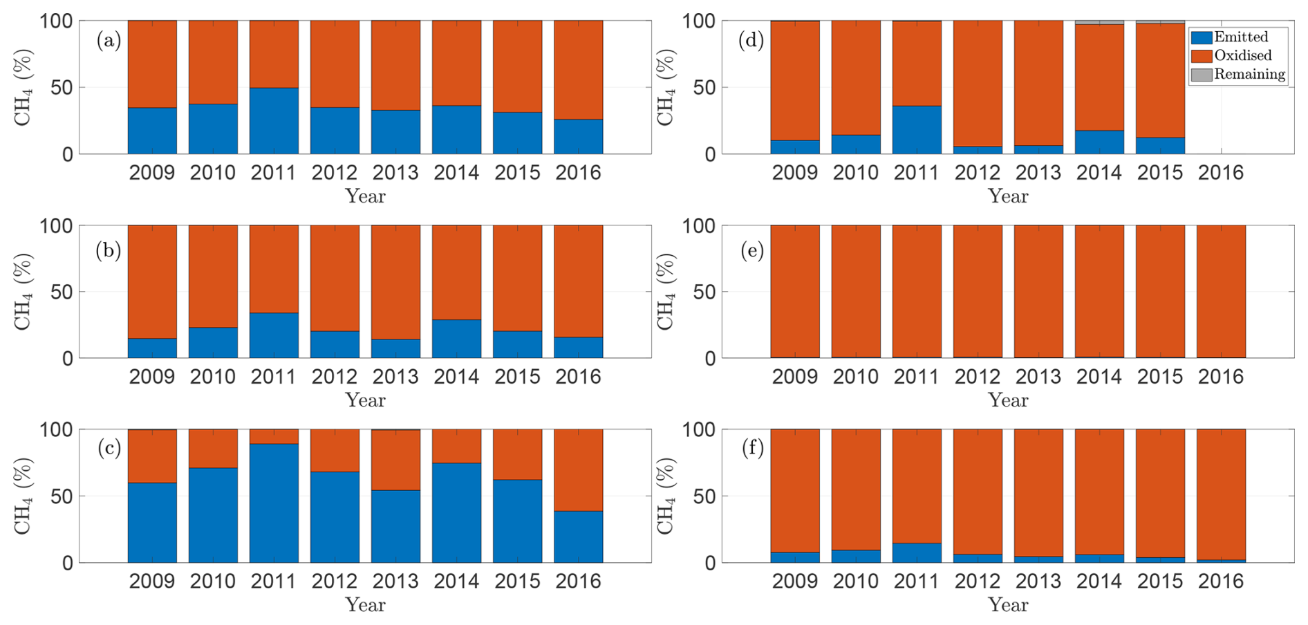
Figure 6 Model predictions of the partitioning of soil CH₄ production into emission, oxidation, and retention over the course of each growing season (2009–2016) for wetlands (a) P1, (b) P3, (c) P8, (d) T5, (e) T6, and (f) T9.

5 Water depth corresponding to maximum emissions

A key contribution of the model developed by Calabrese et al. (2021) was the ability to capture a critical water depth (≈50 cm above the surface) at which CH₄ emissions are maximised due to the interaction between production, oxidation, and transport (see Fig. 1g). Given that our model builds upon their framework, we similarly observe this emergent behaviour, with emissions typically suppressed under both drought and deep inundation. To understand the mechanistic origin and parametric sensitivity of this peak, we examine the steady-state behaviour of the system. Our interpretations of this steady-state are applicable more generally: the governing ODEs for CH₄ dynamics are linear in the CH₄ pool size (Eq. 1) and so the qualitative dependence of emissions on water table depth is partly preserved even at intermediate times. However, this is not always the case – the qualitative behaviour can vary over the time-course of a solution, with the depth at which emissions peak becoming time-dependent depending on input parameters and initial conditions – we defer a detailed exploration of this to future work.

Assuming fixed environmental conditions, the system tends towards a steady-state in the soil column, this corresponds to constant emission fluxes from the soil column (see Eq. 9). The steady-state CH₄ mass in the soil column, $M_s^{*}$, is obtained by setting $\mathrm{d}{M}_s/\mathrm{d}t=\mathrm{0}$ in Eq. (1). Denoting the corresponding emission flux by $f_e^{*}$, we have

$$\begin{array}{}\text{(12)}& f_e^{*}=k_e{M}_s^{*},M_s^{*}={\displaystyle \frac{k_p{f}_b^{\left(p\right)}{f}_T^{\left(p\right)}{f}_w^{\left(p\right)}}{k_o{f}_T^{\left(o\right)}{f}_w^{\left(o\right)}+k_e}}.\end{array}$$

Alternatively, we may write the steady-state emissions as

$$\begin{array}{}\text{(13)}& f_e^{*}=f_p^{*}-f_o^{*},\end{array}$$

with $f_p^{*}$ and $f_o^{*}$ denoting the corresponding production and oxidation rates under fixed environmental conditions. Expressing the system in this form highlights that emissions arise from the balance between production and oxidation, with their differing dependencies on environmental conditions giving rise to emergent emission behaviour.

5.1 Dependence of emissions on water table depth

From Eq. (12), $f_e^{*}$ clearly depends on the water table depth, soil temperature, and on the wetland-specific parameters. To identify the water depth z_p that maximises emissions (for a given set of parameters, temperature, and substrate availability), we solve for the critical point where $\mathrm{d}{f}_e^{*}/\mathrm{d}{z}_w=\mathrm{0}$. In particular, we have

$$\begin{array}{}\text{(14)}& \begin{array}{rl}{\displaystyle }& {\displaystyle \frac{k_p{f}_b^{\left(p\right)}{f}_T^{\left(p\right)}}{{\left(k_o{f}_T^{\left(o\right)}{f}_w^{\left(o\right)}+k_e\right)}^{\mathrm{2}}}}\mathit{\{}{f}_w^{\left(p\right)}{\displaystyle \frac{\mathrm{d}{k}_e}{\mathrm{d}{z}_w}}\left(k_o{f}_T^{\left(o\right)}{f}_w^{\left(o\right)}+k_e\right)\\ {\displaystyle }& {\displaystyle }+k_e\left[{\displaystyle \frac{\mathrm{d}{f}_w^{\left(p\right)}}{\mathrm{d}{z}_w}}\left(k_o{f}_T^{\left(o\right)}{f}_w^{\left(o\right)}+k_e\right)\right.\\ {\displaystyle }& {\displaystyle }\left.-f_w^{\left(p\right)}\left(k_o{f}_T^{\left(o\right)}{\displaystyle \frac{\mathrm{d}{f}_w^{\left(o\right)}}{\mathrm{d}{z}_w}}+{\displaystyle \frac{\mathrm{d}{k}_e}{\mathrm{d}{z}_w}}\right)\right]\mathit{\}}=\mathrm{0},\end{array}\end{array}$$

which simplifies to

$$\begin{array}{}\text{(15)}& \begin{array}{rl}{\displaystyle }& {\displaystyle }{f}_w^{\left(p\right)}{\displaystyle \frac{\mathrm{d}{k}_e}{\mathrm{d}{z}_w}}\left(k_o{f}_T^{\left(o\right)}{f}_w^{\left(o\right)}+k_e\right)\\ {\displaystyle }& {\displaystyle }+k_e\left[{\displaystyle \frac{\mathrm{d}{f}_w^{\left(p\right)}}{\mathrm{d}{z}_w}}\left(k_o{f}_T^{\left(o\right)}{f}_w^{\left(o\right)}+k_e\right)\right.\\ {\displaystyle }& {\displaystyle }\left.-f_w^{\left(p\right)}\left(k_o{f}_T^{\left(o\right)}{\displaystyle \frac{\mathrm{d}{f}_w^{\left(o\right)}}{\mathrm{d}{z}_w}}+{\displaystyle \frac{\mathrm{d}{k}_e}{\mathrm{d}{z}_w}}\right)\right]=\mathrm{0}.\end{array}\end{array}$$

Hence, whilst the dependence of methanogenesis on temperature and substrate govern the overall emission magnitude (Eq. 12), they do not determine the peak location (though this would change if vertical temperature gradients were incorporated).

Given the functional forms of $f_w^{\left(p\right)}$, $f_w^{\left(o\right)}$, and k_e (see Sect. 2), Eq. (15) involves a mixture of exponential and polynomial terms and must be solved numerically for z_w=z_p. For z_w<z_s, we have $\mathrm{d}{f}_e^{*}/\mathrm{d}{z}_w>\mathrm{0}$ for typical parameter ranges and Eq. (15) cannot be satisfied, so peak emissions must always occur at or above the soil surface. For z_w>z_s Eq. (15) yields

$$\begin{array}{}\text{(16)}& \begin{array}{rl}{\displaystyle }& {\displaystyle \frac{-\mathrm{2}D}{(z_w-z_b{)}^{\mathrm{3}}}}(k_o{f}_T^{\left(o\right)}{\mathrm{e}}^{-p_{\mathrm{2}}(z_w-z_b)}+k_{EP}+{\displaystyle \frac{D}{(z_w-z_b{)}^{\mathrm{2}}}})\\ {\displaystyle }& {\displaystyle }+k_e{p}_{\mathrm{2}}{k}_o{f}_T^{\left(o\right)}{\mathrm{e}}^{-p_{\mathrm{2}}(z_w-z_b)}\\ {\displaystyle }& {\displaystyle }-{\displaystyle \frac{k_e{p}_{\mathrm{1}}}{z_w-z_b}}(k_o{f}_T^{\left(o\right)}{\mathrm{e}}^{-p_{\mathrm{2}}(z_w-z_b)}+k_{EP}+{\displaystyle \frac{D}{(z_w-z_b{)}^{\mathrm{2}}}})\\ {\displaystyle }& {\displaystyle }+{\displaystyle \frac{\mathrm{2}D{k}_e}{(z_w-z_b{)}^{\mathrm{3}}}}=\mathrm{0},\end{array}\end{array}$$

or, alternatively:

$$\begin{array}{}\text{(17)}& \begin{array}{rl}{\displaystyle }& {\displaystyle }{k}_o{f}_T^{\left(o\right)}[k_e\left(p_{\mathrm{2}}-{\displaystyle \frac{p_{\mathrm{1}}}{z_w-z_b}}\right)-{\displaystyle \frac{\mathrm{2}D}{(z_w-z_b{)}^{\mathrm{3}}}}]{\mathrm{e}}^{-p_{\mathrm{2}}(z_w-z_b)}\\ {\displaystyle }& {\displaystyle }-{\displaystyle \frac{k_{EP}}{z_w-z_b}}[p_{\mathrm{1}}{k}_e+{\displaystyle \frac{\mathrm{2}D}{(z_w-z_b{)}^{\mathrm{2}}}}]\\ {\displaystyle }& {\displaystyle }+{\displaystyle \frac{D}{(z_w-z_b{)}^{\mathrm{3}}}}\left[\right(\mathrm{2}-p_{\mathrm{1}})k_e-{\displaystyle \frac{\mathrm{2}D}{(z_w-z_b{)}^{\mathrm{2}}}}]=\mathrm{0}.\end{array}\end{array}$$

Whilst one could in principle solve Eq. (17) directly to obtain the depth of peak emissions, the specific functional form of k_e given in Eq. (9) (see also Fig. 1f) simplifies the analysis. For z_w>z_s, the derivative satisfies $\mathrm{d}{k}_e/\mathrm{d}{z}_w\approx \mathrm{0}$, so the first term on the left-hand side of Eq. (15) can be neglected. A practical approximation is therefore obtained by solving the more interpretable equation

$$\begin{array}{}\text{(18)}& \begin{array}{rl}{\displaystyle }& {\displaystyle }{k}_o{f}_T^{\left(o\right)}\left(p_{\mathrm{2}}-{\displaystyle \frac{p_{\mathrm{1}}}{z_w-z_b}}\right){\mathrm{e}}^{-p_{\mathrm{2}}(z_w-z_b)}\\ {\displaystyle }& {\displaystyle }-{\displaystyle \frac{p_{\mathrm{1}}{k}_{EP}}{z_w-z_b}}+{\displaystyle \frac{(\mathrm{2}-p_{\mathrm{1}})D}{(z_w-z_b{)}^{\mathrm{3}}}}=\mathrm{0}.\end{array}\end{array}$$

The accuracy of this reduced formulation is illustrated in Fig. 7 (red crosses), which shows excellent agreement with solutions to Eq. (17) (black lines).

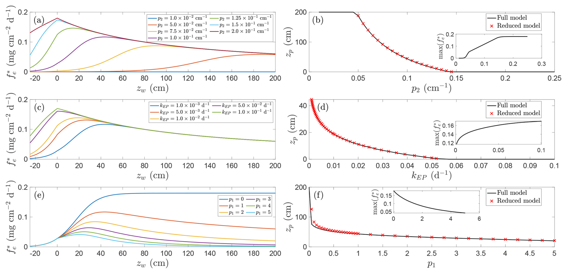
Figure 7 Relationship between CH₄ emissions and water table depth for different parameter families. Panels (a, b) show effect of varying p₂, panels (c, d) show effect of varying k_EP and panels (e, f) show effect of varying p₁. Left panels (a, c, e) show representative solutions, right panels (b, d, f) show location of emission peak as a function of varied parameter (insets show magnitude of this peak). Red crosses indicate approximation found by solving Eq. (18). Unless otherwise indicated parameters are $k_p=\mathrm{1.0}\mathrm{mg}{\mathrm{CH}}_{\mathrm{4}}{\mathrm{cm}}^{-\mathrm{2}}{\mathrm{d}}^{-\mathrm{1}}$, p₁=1.0, $k_o=\mathrm{2.0}\times {\mathrm{10}}^{\mathrm{2}}{\mathrm{d}}^{-\mathrm{1}}$, $p_{\mathrm{2}}=\mathrm{1.0}\times {\mathrm{10}}^{-\mathrm{1}}{\mathrm{cm}}^{-\mathrm{1}}$, Q_p=5.0, p₃=1, Q_o=1.5, $z_b=-\mathrm{1.0}\times {\mathrm{10}}^{-\mathrm{2}}\mathrm{cm}$, $k_{EP}=\mathrm{1.0}\times {\mathrm{10}}^{-\mathrm{2}}{\mathrm{d}}^{-\mathrm{1}}$, p₅=2.0, T=20 °C, and NDVI=0.8.

The existence of a positive root requires that the sum of the positive terms outweighs the negative ones for z_w>z_s; otherwise, provided p₁≠0, emissions are maximised at the soil surface (i.e. z_p=0). These dependencies may be able to explain conflicting conclusions for optimal water depth for emissions. For example, Zhang et al. (2024) report exponential decay in CH₄ emission fluxes with water depth above the surface, which contrasts with the data synthesis performed by Calabrese et al. (2021); this may result from stronger oxidation or weaker plant transport in the wetlands studied by Zhang et al. (2024). Similarly, Taylor et al. (2023) report that water depth for peak emissions depends on the wetland type (e.g. bog vs. fen).

5.2 Critical water depth dependence on model parameters

Equation (18) reflects a balance of competing effects: the exponential decline in oxidation against the hyperbolic decay in production with depth (first term), plant-mediated transport (second term), and diffusion (third term). Since the diffusion term depends strongly on depth, its relative influence diminishes when z_w−z_b is large. Furthermore, if p₁>2 and $p_{\mathrm{1}}>(z_w-z_b)p_{\mathrm{2}}$, no positive solution exists and emissions peak at the surface, driven by the rapid decline in production with depth. Other parameter combinations can also preclude a solution, depending on how oxidation is modulated by temperature and other environmental factors (see discussion in Sect. 5.3).

We explore these dependencies in Fig. 7, which shows, for fixed baseline parameters, the influence of (a, b) the oxidation decay rate, (c, d) plant transport and ebullition, and (e, f) production decay on peak emission depth. The chosen parameters correspond to those identified as influential by means of a Morris sensitivity analysis (Appendix B). Figure 7a, c, and e display representative CH₄ flux curves for different parameter families, whilst panels (b), (d), and (f) plot the associated peak depths (insets show the corresponding maximum emission rate).

The physical interpretation follows directly from the functional forms in Fig. 1. Methane production is highest at the soil surface, rising as the water table approaches the surface as more of the soil column is exposed to anoxic conditions favourable to methanogenesis but declining when the soil column becomes deeply inundated because of substrate dilution. In contrast, oxidation decreases exponentially with depth and diffusive release scales approximately as an inverse square of water depth. When the oxidation decay rate p₂ increases, the aerobic oxidation zone quickly collapses with water depth and CH₄ is consumed less efficiently. As a result, the emission peak shifts upward toward the soil surface and the total flux rises by orders of magnitude (Fig. 7a and b). At the extreme of large p₂ the model predicts almost no oxidation, so production nearly completely controls the flux and the peak coincides with the soil surface (Fig. 7a and b); in particular, in this regime deep inundation is not required to limit CH₄ consumption.

Meanwhile, increasing plant-mediated transport and ebullition produces a similar but more modest effect, shifting both the location and magnitude of the emission peak. Greater ebullition and plant transport allow CH₄ to rapidly bypass the oxic layer, further reducing the role of oxidation. Since these pathways are largely independent of water depth, and diffusion is weak above the surface, the overall flux pattern is increasingly determined by the near-surface production profile: higher transport rates both increase emission magnitude and move the peak closer to the surface (Fig. 7c and d), as transport outcompetes oxidation of CH₄ produced in the soil column. In particular, as the dominant emission pathway shifts from diffusion, which decays with water depth, to constant ebullition and plant transport, emissions become more directly governed by production. Wetlands with abundant emergent vegetation therefore tend to exhibit higher fluxes and shallower emission peaks. As these emission routes depend directly on the total CH₄ present in the soil column, a reinforcing feedback occurs: higher emissions deplete CH₄ available for future release, further shifting the peak toward the soil surface where production is maximal.

The influence of production decay is subtler in magnitude but far more significant for peak location. For instance, when p₁=0, peak emissions occur at z_w→∞, with emissions effectively plateauing with increasing inundation, consistent with the absence of depth-dependent decline in production and continued loss of CH₄ via oxidation (this balance can also be readily observed in Eq. 18, which becomes strictly positive). As p₁ increases, deeper water no longer offsets oxidation because production itself is suppressed; the emission maximum therefore migrates toward the soil surface (Fig. 7e and f). This behaviour can also be inferred from the simplified analytical condition (Eq. 18), which becomes strictly positive when p₁=0.

These results explain why a deeper wetland can sometimes emit less CH₄ than a shallower one when oxidation remains active, whereas wetlands rich in organic carbon, such as agricultural systems, can become largely anoxic and release much more CH₄. They also show that increasing plant-mediated transport, ebullition, or substrate availability consistently raises emissions and shifts the peak toward the soil surface. In contrast, extending the oxidation decay length suppresses fluxes by enlarging the aerobic consumption zone.

5.3 Critical water depth dependence on temperature

A notable consequence of Eqs. (17) and (18) is that the peak location is itself temperature-dependent via $f_T^{\left(o\right)}$, implying that both the magnitude and position of peak emissions shift throughout the growing season in response to a shifting balance between production and oxidation. Figure 8 illustrates this dependence: panel (a) shows CH₄ fluxes at fixed temperatures, whilst panel (b) plots the corresponding peak emission depths and flux magnitudes. As temperature increases, both the intensity of emissions and the depth at which they peak typically rise, shifting the emission maximum further above the soil surface. This behaviour reflects the fact that warming generally amplifies CH₄ production throughout the inundated column more strongly than it enhances oxidation (see also Fig. 6), so that the net flux maximum tends to occur at progressively higher positions above the soil surface. However, under some parameter choices, in particular when $p_{\mathrm{1}}>p_{\mathrm{2}}(z_w-z_b)$, the temperature-driven increase in oxidation can instead shift the peak closer to the soil surface. Since this typically occurs only when z_w−z_b is small and p₁ is large, it is usually a weaker effect.

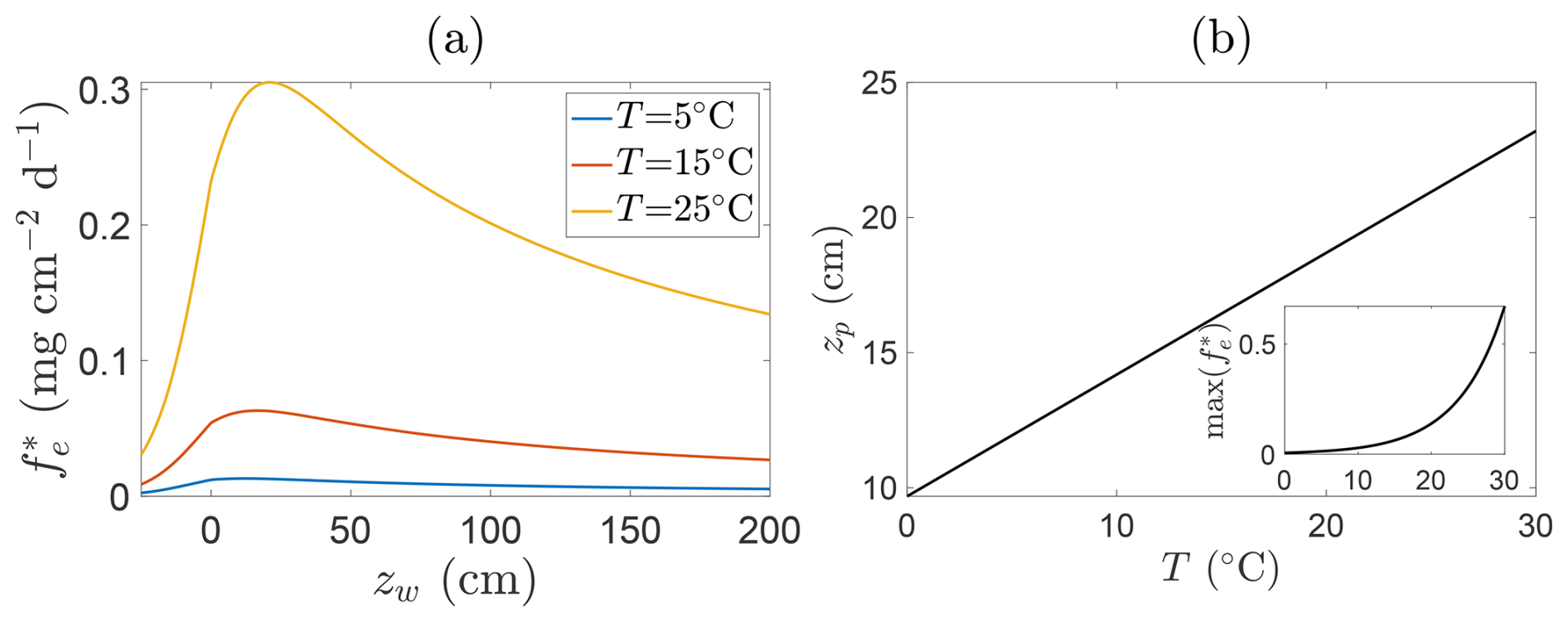
Figure 8 Relationship between CH₄ emissions and water table depth for fixed parameters and different soil temperatures. Panel (a) shows representative solutions at T=5 °C (blue line), T=15 °C (orange line), and T=25 °C (yellow line) of steady state emissions fluxes against water table depth. Panel (b) shows location of emission peak as a function of temperature (insets show magnitude of this peak). Parameters are $k_p=\mathrm{1.0}\mathrm{mg}{\mathrm{CH}}_{\mathrm{4}}{\mathrm{cm}}^{-\mathrm{2}}{\mathrm{d}}^{-\mathrm{1}}$, p₁=1.0, $k_o=\mathrm{2.0}\times {\mathrm{10}}^{\mathrm{2}}{\mathrm{d}}^{-\mathrm{1}}$, $p_{\mathrm{2}}=\mathrm{1.0}\times {\mathrm{10}}^{-\mathrm{1}}{\mathrm{cm}}^{-\mathrm{1}}$, Q_p=5.0, p₃=1, Q_o=1.5, $z_b=-\mathrm{1.0}\times {\mathrm{10}}^{-\mathrm{2}}\mathrm{cm}$, $k_{EP}=\mathrm{1.0}\times {\mathrm{10}}^{-\mathrm{2}}{\mathrm{d}}^{-\mathrm{1}}$, p₅=2.0, and NDVI=0.8.

This temperature sensitivity carries broader implications. As global temperatures rise, wetlands may exhibit not only higher CH₄ emissions but also shifts in the vertical structure of those emissions. Such changes could impact the efficacy of interventions aimed at suppressing emissions, particularly those based on manipulating water levels. Optimal water levels for mitigation may vary substantially across seasons or under future climatic conditions, necessitating adaptive, site-specific strategies.

6 Discussion

In this paper we have presented a simple zero-dimensional model to describe the response of wetland CH₄ emissions to variations in water depth, temperature, and vegetation-derived substrate input. This work refines and extends the framework of Calabrese et al. (2021) by demonstrating how seasonal fluctuations in these environmental drivers modulate the balance between methanogenesis and oxidation, thereby shaping both the magnitude of peak methane emissions and the conditions under which this peak occurs. In particular, the model reveals that strong oxidative capacity within the wetland column can substantially mitigate CH₄ emissions by acting as an effective sink for produced CH₄, an effect most pronounced in temporarily inundated wetlands. The model thus provides a mechanistic basis for understanding seasonal emission patterns and assessing the combined influence of environmental controls on wetland CH₄ fluxes. Although intentionally simple, a fully mechanistic, higher-dimensional representation would require detailed parameterisation and extensive process-level data. In contrast, our model offers a computationally efficient yet physically informed approach that captures the essential dependencies governing CH₄ production and emission dynamics.

A key emergent outcome of the non-linear interaction between methanogenesis, oxidation, and transport identified by our model is an intermediate critical water depth at which CH₄ emissions are maximised (such a peak has also been identified by Calabrese et al., 2021, but is inaccessible using other models based solely on subsurface water tables). Although derived under a steady-state assumption, this analysis provides valuable insight into system behaviour at intermediate times, particularly because the governing ODEs are linear in CH₄ pool size. We isolate the key parameters controlling both the magnitude and position of this emission peak – specifically, the exponential decay of oxidation, the hyperbolic decay of production, plant-mediated transport and ebullition, and diffusion. We examine how these processes interact to shape emission profiles (see Fig. 7), complemented by a global sensitivity analysis in Appendix B. Importantly, we show that in some wetlands the depth of peak emissions is temperature-dependent, reflecting the modulation of oxidation rates by seasonal temperature changes. This indicates that optimal water levels for maximal CH₄ fluxes can vary over the growing season or under different climate scenarios, highlighting the potential necessity for seasonally adaptive management strategies.

This understanding is facilitated by the model’s simple zero-dimensional structure, which provides a computationally efficient alternative to more complex, spatially explicit PDE-based models. However, limitations emerge when the water table falls below the soil surface, potentially reflecting either a breakdown of the zero-dimensional approximation in this regime or the coarse method used to estimate water depth (see Sect. 3.1). Nevertheless, emissions under these conditions are generally small compared to those during saturated or inundated periods, so any overestimation has limited impact on total seasonal budgets. Improving model performance during low-water periods would nonetheless broaden its applicability beyond wetland centres, enabling predictions across spatially heterogeneous landscapes where water table depth varies substantially with soil profile (wetland bathymetry). Such an extension would support more accurate, large-scale assessments of wetland CH₄ emissions.

Beyond water table depth, soil temperature and substrate availability, wetland CH₄ emissions are controlled by a host of additional environmental and anthropogenic factors. Alternative electron acceptors such as nitrate and sulphate can suppress emissions by supporting more energetically favourable microbial pathways. Soil pH and salinity also modulate emission pathways: acidic soils favour hydrogenotrophic methanogenesis, whilst saline coastal wetlands tend to exhibit reduced CH₄ production (Poffenbarger et al., 2011). Microbial community composition also varies between sites, with acetoclastic-dominated communities showing particularly strong seasonal responses (Angle et al., 2017). Wetland hydrology also plays an important role, with flooding duration and frequency influencing oxygen availability and nutrient loading. Similarly, wetland morphology controls emissions, with larger wetlands (i.e. those with greater wetland volume to surface area) typically exhibiting lower emissions. Anthropogenic impacts, such as drainage and pollution, further alter water levels and chemical properties. In our model, we do not explicitly account for these complexities, assuming their effects are roughly constant and encapsulated in the site-specific calibration parameter, k_p. Whilst this is a simplification, our model successfully predicts both seasonal and inter-annual variations in fluxes, capturing peaks and troughs and producing accurate estimates of total seasonal emissions (see Figs. 3–5). This performance is achieved without explicitly modelling these secondary processes, suggesting that the primary drivers considered are sufficient to reproduce leading-order emission dynamics. Hence, our model provides a minimal mechanistic framework for estimating CH₄ emissions and identifying environmental conditions that favour elevated fluxes. It also facilitates emission estimates under unobserved or data-sparse environmental scenarios.

Another simplification we employ is to lump the hydrogenotrophic, acetoclastic, and methylotrophic methanogenesis pathways into a single effective production term. Whilst these pathways differ in substrate requirements and temperature sensitivities (e.g. hydrogenotrophic methanogenesis typically dominating deeper in the soil and early in the season, and acetoclastic methanogenesis prevailing near the surface later in the season) this aggregation enables the model to capture their common dependence on biomass and temperature without introducing additional complexity. However, by not resolving these pathways separately, the model cannot explicitly reproduce seasonal hysteresis effects that may arise when the dominant methanogenic pathway shifts over the growing season (Chang et al., 2019, 2021). This trade-off provides further opportunity for refinement in future work: explicitly modelling both pathways could help capture asymmetric seasonal responses in CH₄ emissions more accurately.

We have validated the model against a representative set of mid-latitude wetlands in the PPR, a sensible starting point given their ecological and hydrological diversity and the availability of extensive observational data. However, further evaluation is necessary to assess model performance in other mid-latitude regions and, critically, in tropical and high-latitude wetlands to determine its generalisability. Future model developments should incorporate biomass accumulation and decay dynamics, more realistic representations of ebullition and plant-mediated gas transport, and potentially CO₂ dynamics, which may also affect methanogenesis via hydrogenotrophic pathways. Additionally, coupling the model with a stochastic representation of water table fluctuations – driven by rainfall and evapotranspiration – would facilitate investigations into how climate change, through warming-induced increases in evapotranspiration and methanogenesis alongside elevated water tables due to intensified rainfall, may alter emission patterns. Such advancements are essential for informing future wetland management strategies. In particular, whilst soil temperature and substrate availability are difficult to manipulate, water depth can be controlled through drainage, making understanding its influence on peak emissions critical for wetland management.

Appendix A: Parameter ranges

Table A1 Optimised parameters employed in simulations for the centre of wetlands P1, P3, P8, T5, T6, T9.

In Table A2 we present the allowable parameter ranges for each model parameter employed throughout the paper based on existing literature.

(Dalcin Martins et al., 2017)Calabrese et al. (2021)Calabrese et al. (2021)Bender and Conrad (1992)Calabrese et al. (2021)Zhang et al. (2002); Souza et al. (2021)Walter and Heimann (2000)(Van Hulzen et al., 1999; Segers, 1998; Dunfield et al., 1993)Dunfield et al. (1993)Zhang et al. (2002)Calabrese et al. (2021)Bansal et al. (2023b)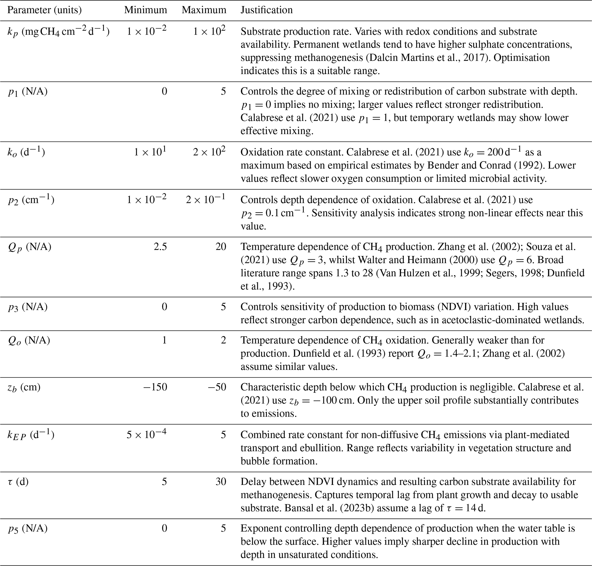

Table A2 Model parameter ranges.

Appendix B: Sensitivity analysis

Despite efforts to minimise the number of model parameters whilst retaining essential geochemical processes, even this simplified model remains highly parameterised. When applied across large wetland landscapes, site-specific calibration becomes impractical. Instead, it is more realistic to represent landscape heterogeneity through parameter distributions. Some parameters assumed constant may also vary over time. For instance, the CH₄ production rate k_p likely depends on salinity, which fluctuates with freshwater inputs and discharge. Parameter sensitivity is further context-dependent: under persistently high water tables, oxidation parameters may have little effect, whereas under drier conditions they can dominate. Given this complexity, understanding which parameters most strongly influence model behaviour is therefore critical, particularly since several remain poorly constrained in the literature.

B1 Morris method

To assess the sensitivity of our model outputs to input parameters, we employ the Morris method, a global screening technique well-suited to computationally expensive models. This method efficiently identifies parameters that exert significant influence on the output, exploring the parameter space broadly by evaluating many one-at-a-time perturbations across multiple regions of the domain.

A detailed description of the Morris method is provided in Morris (1991); Stadt and Layton (2024); here we summarise the key steps. Let $f(X_{\mathrm{1}},X_{\mathrm{2}},\mathrm{\dots },X_n)$ denote the model output for the parameter set $(X_{\mathrm{1}},X_{\mathrm{2}},\mathrm{\dots },X_n)$. All parameters are rescaled to the unit interval [0,1] and discretised into p levels, with perturbation step $\mathit{\delta }=\mathrm{1}/(p-\mathrm{1})$. In subsequent simulations each parameter is varied within ±25 % of its baseline dimensional value, and the perturbations in the rescaled space are mapped back to dimensional units before evaluation.

Starting from an initial parameter set, the model is sequentially perturbed in one parameter at a time to compute the elementary effects:

$$\begin{array}{}\text{(B1)}& \begin{array}{rl}{\displaystyle }& {\displaystyle }{\text{EE}}_i\\ {\displaystyle }& {\displaystyle }={\displaystyle \frac{f(X_{\mathrm{1}},\mathrm{\dots },X_i+{\mathrm{\Delta }}_i,\mathrm{\dots },X_n)-f(X_{\mathrm{1}},\mathrm{\dots },X_i,\mathrm{\dots },X_n)}{{\mathrm{\Delta }}_i}},\end{array}\end{array}$$

repeating the process for all n parameters across r random trajectories (r=100 in this study). From the ensemble of ${\text{EE}}_i^{\left(k\right)}$ values, the sensitivity indices are computed as

$$\begin{array}{}\text{(B2)}& \begin{array}{rl}{\displaystyle }{\mathit{\mu }}_i& {\displaystyle }={\displaystyle \frac{\mathrm{1}}{r}}{\sum }_{k=\mathrm{1}}^r{\text{EE}}_i^{\left(k\right)},{\mathit{\mu }}_i^{*}={\displaystyle \frac{\mathrm{1}}{r}}{\sum }_{k=\mathrm{1}}^r\left|{\text{EE}}_i^{\left(k\right)}\right|,\\ {\displaystyle }{\mathit{\sigma }}_i& {\displaystyle }=\sqrt{{\displaystyle \frac{\mathrm{1}}{r}}{\sum }_{k=\mathrm{1}}^r({\text{EE}}_i^{\left(k\right)}-{\mathit{\mu }}_i{)}^{\mathrm{2}}},M_i=\sqrt{{\mathit{\mu }}_i^{\mathrm{2}}+{\mathit{\sigma }}_i^{\mathrm{2}}}.\end{array}\end{array}$$

representing the mean, mean absolute, standard deviation, and combined Morris index, respectively; ${\mathit{\mu }}_i^{*}$ indicates the overall importance of parameter X_i, whilst σ_i reflects interaction or non-linearity.

To facilitate comparison across parameters of different magnitudes, we also apply the relative Morris method, in which each elementary effect is normalised by its baseline value:

$$\begin{array}{}\text{(B3)}& {\text{EE}}_i^r={\displaystyle \frac{X_i}{f(X_{\mathrm{1}},\mathrm{\dots },X_n)}}{\text{EE}}_i,\end{array}$$

yielding corresponding statistics ${\mathit{\mu }}_i^{r*}$, ${\mathit{\sigma }}_i^r$, and $M_i^r$. This formulation expresses the response as a fractional change in output relative to a fractional change in input, allowing fairer comparison across parameters. We report both absolute and relative indices to identify parameters with the greatest absolute or proportional influence on model output.

B2 Sensitivity of emission fluxes to parameters

We assess the sensitivity of steady-state CH₄ emission fluxes to model parameters in Fig. B1. Under fixed environmental conditions (NDVI=0.5, T=15 °C, and z_w=25 cm), Fig. B1a shows results from both the absolute and relative (normalised) Morris analyses. Panel (a) presents the scatter plot of σ against μ^* for each parameter, whilst Fig. B1b shows the corresponding Morris index; panels (c) and (d) present the relative counterparts.

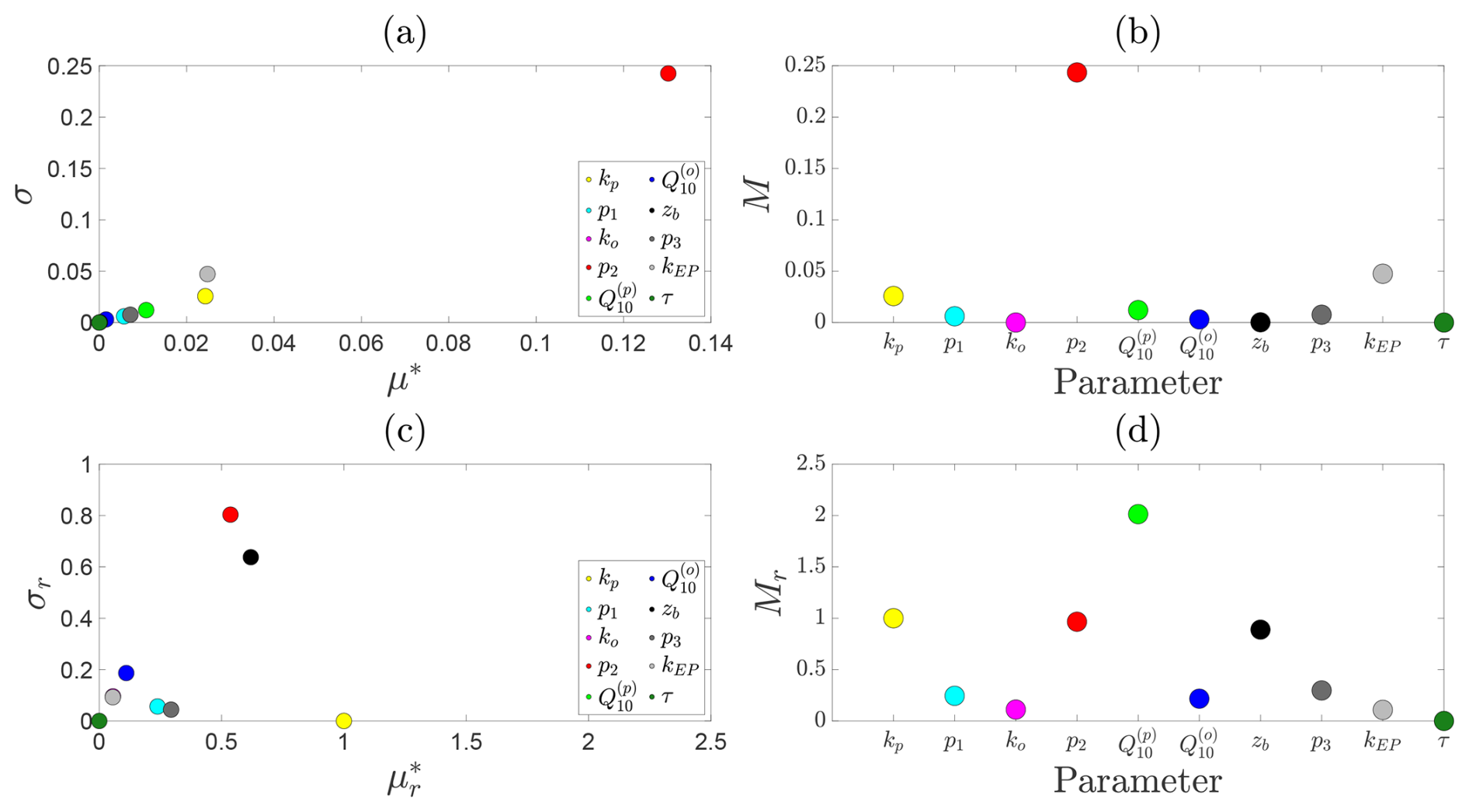
Figure B1 Sensitivity analysis of predicted steady-state CH₄ emission fluxes. For a fixed water depth of 25 cm: (a) mean absolute (${\mathit{\mu }}_i^{*}$) versus standard deviation (σ_i) of elementary effects for each parameter; (b) corresponding ranked Morris indices. Panels (c) and (d) show the same results for the relative (normalised) Morris analysis.

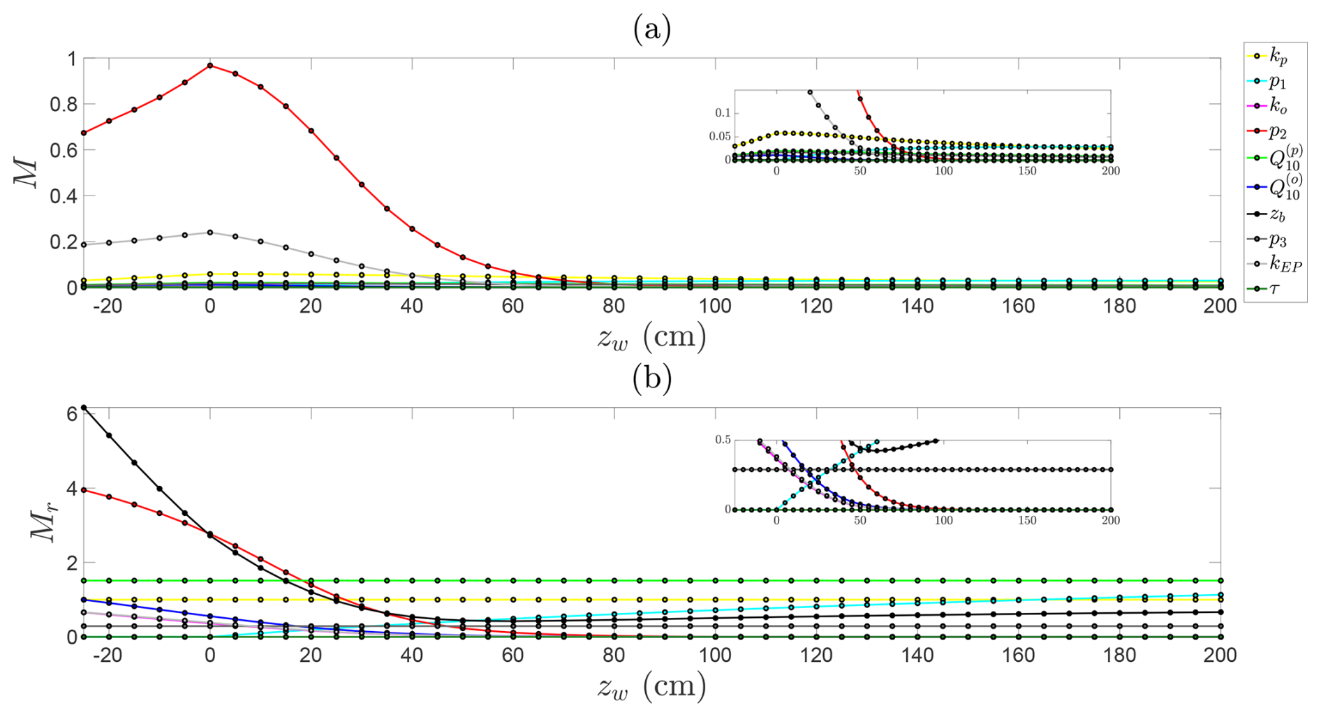
Figure B2 Sensitivity analysis of predicted steady-state CH₄ emission fluxes across water table depths, with constant NDVI and temperature. (a) Absolute Morris indices and (b) relative (normalised) Morris indices for each parameter as a function of water depth.

At this moderate water table depth, the dominant absolute controls on CH₄ emissions are the decay rate of oxidation with water table depth, followed by the ebullition and plant-mediated transport rates. These parameters primarily govern the pathways through which CH₄ escapes the soil column, rather than its production. This is consistent with the relatively weak hyperbolic decay of production with water table depth compared to the sharp exponential decline in oxidation with increasing inundation. In contrast, the relative Morris analysis highlights a different picture: $Q_{\mathrm{10}}^{\left(p\right)}$ emerges as a key control on CH₄ dynamics, reflecting its strong influence on temperature-dependent methanogenesis under these moderate conditions. Secondary relative sensitivities are found for k_p, p₂, and z_b, which together regulate CH₄ production, oxidation, and the effective soil volume available for methanogenesis. These collectively shape both the magnitude and spatial extent of CH₄ generation and oxidation within the soil column.

To explore how parameter sensitivities change across hydrological regimes, we examine absolute and relative Morris indices for each parameter across water table depths from 25 cm below to 200 cm above the soil surface (Fig. B2). A clear transition emerges in the dominant controls on CH₄ emissions. When the water table is below the soil surface, aerobic conditions favour oxidation, and sensitivity is highest to the oxidation decay rate (p₂) and the constant emission rate from the soil column (k_EP). As the water table rises above the surface, the influence of oxidation declines sharply; under anaerobic conditions, CH₄ largely escapes unoxidised, rendering oxidation dynamics negligible (see insets in Fig. B2). Under these inundated conditions, emissions are instead controlled by methanogenesis and transport parameters, particularly ebullition and plant-mediated flux rates, and the hyperbolic decay term in CH₄ production, which has no effect when the water table lies below the surface. The relative Morris analysis (Fig. B2b) additionally highlights the dominant role of the contributing soil depth (z_b), which determines the volume of soil participating in production, oxidation, and emission, and is therefore consistently influential when the water table is near or below the surface. Under deeper water table conditions, CH₄ production in the soil column becomes the primary determinant of emissions. In this regime, the top three controls are $Q_{\mathrm{10}}^{\left(p\right)}$, p₁, and k_p, reflecting strong temperature sensitivity, the production decay with water table depth, and the base production rate. Produced CH₄ is largely released at a constant rate via plant-mediated transport and ebullition.

Overall, the sensitivity analysis highlights how the dominant controls on CH₄ emissions shift with hydrological regime and demonstrate the need to prioritise accurate representation of different parameters under these regimes. When the water table lies near or below the soil surface, oxidation-related parameters are most critical, whereas production-related parameters dominate when the water table is high above the soil surface.