Subsurface dissolution reduces the efficiency of mineral-based open-ocean alkalinity enhancement

Carbon dioxide removal (CDR) from the atmosphere will likely be required to offset hard-to-abate emissions and limit global warming to well below 2 °C, in line with the Paris Agreement. Among proposed CDR strategies, ocean alkalinity enhancement (OAE) is increasingly discussed because it offers high carbon sequestration potential, long storage timescales, and potentially mitigates ocean acidification. OAE is often envisioned to occur in the open ocean through the dissolution of alkaline mineral powders, such as forsterite, the most abundant form of olivine. Fine-grained powders dissolve near the surface, where the added alkalinity can efficiently enhance oceanic carbon uptake, whereas coarser grains sink and dissolve at depth. Most modeling studies assume complete surface dissolution, leaving the impact of subsurface dissolution on ocean carbon uptake poorly understood. Here, we develop idealized vertical mineral dissolution profiles that vary with environmental conditions and grain size. These profiles are implemented in a comprehensive Earth system model to assess the capture efficiency of OAE, defined as the additional carbon taken up by the ocean per alkalinity added. We find that the efficiency is very sensitive to grain size and may decrease by more than 75 % when grain size doubles, as larger grains release the alkalinity at deeper depth. Efficiency further decreases when particles are not uniformly sized but follow a particle size distribution with the same mean particle volume. In addition, efficiency is time-dependent: it is lower in the first decades of OAE and increases as alkalinity previously released in the ocean interior eventually resurfaces, often far from deployment sites. For forsterite particles with diameter 3.4 µm, the efficiency is less than one-fourth of that achieved with surface alkalinity addition over the first decade, less than one-third over the first 30 years, and less than half over 175 years. Our results indicate that forsterite grain sizes would need to be around 1.7 µm to achieve effective open-ocean alkalinity enhancement and that monitoring, reporting, and verification would be challenged by delayed and spatially dispersed carbon uptake, questioning the suitability of olivine. Minerals with faster dissolution rates may present more viable alternatives when mineral particle properties are closely controlled.

1 Introduction

Carbon dioxide removal (CDR) is widely considered necessary for achieving net-zero CO₂ emissions targets and limiting global warming in line with the Paris Agreement (Babiker et al., 2022). Among various CDR approaches, marine-based methods have gained growing scientific and policy interest. In particular, ocean alkalinity enhancement (OAE) has emerged as a promising option due to its well-understood carbonate chemistry, high carbon sequestration potential, long storage timescales (Boyd and Vivian, 2019; Canadell et al., 2021), and its potential for ocean acidification mitigation (Doney et al., 2025).

OAE is often thought to be implemented by adding alkaline mineral powders, such as the silicate mineral olivine, to the open ocean surface, where dissolution increases seawater alkalinity and enhances carbon uptake from the atmosphere (Köhler et al., 2010; National Academies of Sciences, Engineering, and Medicine, 2022). Global modeling studies of OAE commonly assume instantaneous and complete alkalinity release at the surface of the open ocean (Keller et al., 2014; Nagwekar et al., 2024; Schwinger et al., 2024; Tyka, 2025; Zhou et al., 2025; Nagwekar et al., 2026) or coastal ocean (Feng et al., 2017; He and Tyka, 2023). However, this assumption holds only if the added minerals dissolve rapidly, which depends strongly on particle size (Boyd and Vivian, 2019; National Academies of Sciences, Engineering, and Medicine, 2022). Outside shallow and well-mixed coastal waters, slowly dissolving coarser particles sink quickly, releasing alkalinity at depth rather than near the surface. Alkalinity released in the ocean interior contributes to oceanic carbon uptake only when those waters re-emerge at the surface, a process that can take decades to centuries depending on the regional ocean ventilation timescales. Conversely, grinding minerals to finer sizes increases dissolution rates but comes at the cost of higher life-cycle energy demand and associated CO₂ emissions (Foteinis et al., 2023).

A few studies have analyzed the mineral dissolution dynamics, particularly for the silicate mineral olivine, using simplified analytical shrinking core models that idealize mineral particles as smooth spheres (Hangx and Spiers, 2009). These models have been used to estimate dissolution times and carbon uptake in coastal OAE settings (Hangx and Spiers, 2009; Feng et al., 2017) and to approximate alkalinity release within the surface mixed layer of the open ocean (Köhler et al., 2013; Renforth and Kruger, 2013; Yang et al., 2025). In contrast, Fakhraee et al. (2023) employed a complex mineral particle model to simulate alkalinity release in an Earth system model of reduced complexity and coarse spatial resolution. These studies show that dissolution time increases strongly with particle size, highlight regional differences in mixed layer alkalinity release, and identify potential interactions between seeded particles and planktonic communities. Nevertheless, we currently lack knowledge about the impact of particle sinking during dissolution on OAE efficiency, which needs to be assessed with ocean-biogeochemical models or Earth system models.

Here, we analyze the efficiency of mineral-based OAE using a comprehensive, fully coupled Earth system model that explicitly accounts for the interplay between particle sinking and dissolution, represented through a shrinking core model (Hangx and Spiers, 2009). We derive simple analytical vertical alkalinity release profiles and apply them as boundary conditions to the Earth system model. The analysis focuses on the influence of particle size, particle size distribution, and deployment location on alkalinity release and OAE-induced carbon uptake. We mainly discuss the alkaline mineral olivine, often considered for its relatively high dissolution rate compared to other silicate minerals, and also draw a comparison to the faster dissolving mineral brucite. Following the CDRMIP protocol (Keller et al., 2018), mineral powders are homogeneously added to the world ocean, totaling to 4.92Gt forsterite (the most abundant form of olivine) or 4.08Gt brucite per year. For both minerals, the current annual world production is on the order of a few Mt yr⁻¹ (Caserini et al., 2022), highlighting the idealized character of the model experiment. Section 2 describes the alkalinity release profiles, the treatment of varying environmental conditions for these profiles, as well as the experimental design for the Earth system model. Section 3 presents the resulting regional variations in the vertical alkalinity release profiles and quantifies the sensitivity of carbon uptake efficiency to particle size, both for uniform particles and a particle size distribution. The results and their limitations are discussed in Sect. 4.

2 Methods

2.1 Alkalinity release profiles

2.1.1 Particle dissolution in the shrinking core model

We consider spherical particles with a dissolution rate that is proportional to the surface area (constant area-normalized dissolution rate r in $\mathrm{mol}{\mathrm{m}}^{-\mathrm{2}}{\mathrm{s}}^{-\mathrm{1}}$). The decrease in the number of moles of the mineral stored in the particle N_p per time is given by the product of r and the surface area A:

$$\begin{array}{}\text{(1)}& {\displaystyle \frac{\mathrm{d}{N}_{\mathrm{p}}}{\mathrm{d}t}}=-r\cdot A\end{array}$$

As a result, the particle diameter (d) decreases linearly with time (see also Hangx and Spiers, 2009):

$$\begin{array}{}\text{(2)}& {\displaystyle \frac{\mathrm{d}d}{\mathrm{d}t}}=\underset{=\mathrm{2}/A}{\underbrace{{\displaystyle \frac{\mathrm{d}d}{\mathrm{d}V}}}}\cdot \underset{=V_{\text{mol}}}{\underbrace{{\displaystyle \frac{\mathrm{d}V}{\mathrm{d}{N}_{\mathrm{p}}}}}}\cdot {\displaystyle \frac{\mathrm{d}{N}_{\mathrm{p}}}{\mathrm{d}t}}=-\mathrm{2}r{V}_{\text{mol}}\end{array}$$

with V_mol as the molar volume of the mineral (the molar mass of the mineral divided by its density). Such a simple particle dissolution model is referred to as a shrinking core model. When this particle is sinking with speed v_sink during dissolution, the change in N_p per depth is given by the change per time divided by sinking speed:

$$\begin{array}{}\text{(3)}& {\displaystyle \frac{\mathrm{d}{N}_{\mathrm{p}}}{\mathrm{d}z}}={\displaystyle \frac{\mathrm{d}{N}_{\mathrm{p}}}{\mathrm{d}t}}\cdot {\displaystyle \frac{\mathrm{1}}{v_{\text{sink}}}}=-{\displaystyle \frac{r\cdot A}{v_{\text{sink}}}}.\end{array}$$

The term v_sink is the Stokes settling velocity of a sinking spherical particle of diameter d,

$$\begin{array}{}\text{(4)}& v_{\text{sink}}={\displaystyle \frac{({\mathit{\rho }}_{\mathrm{p}}-{\mathit{\rho }}_{\mathrm{w}})g{d}^{\mathrm{2}}}{\mathrm{18}\mathit{\mu }}},\end{array}$$

with the gravitational acceleration g, particle density ρ_p, seawater density ρ_w, and the dynamic viscosity of seawater μ. Since both v_sink and the particle surface area A=πd² are proportional to d², the dependence of $\mathrm{d}{N}_{\mathrm{p}}/\mathrm{d}z$ on d cancels out and $\mathrm{d}{N}_{\mathrm{p}}/\mathrm{d}z$ does not change with particle size. Therefore, larger particles release more alkalinity per unit time due to their larger surface area but also sink faster, such that they lose the same number of moles per depth as smaller particles.

Figure 1 Alkalinity release profiles for (a) uniform particles (Sect. 2.1.2) and (b) for particles with an exponential particle size distribution (Sect. 2.1.3).

The penetration depth z₀ is the depth at which a particle with an initial diameter d is completely dissolved. It is given by

$$\begin{array}{}\text{(5)}& z_{\mathrm{0}}=\underset{V_{\mathrm{d}}/V_{\text{mol}}}{\underbrace{N_{\mathrm{p}}\left(\mathrm{0}\right)}}/\left(-{\displaystyle \frac{\mathrm{d}{N}_{\mathrm{p}}}{\mathrm{d}z}}\right)={\displaystyle \frac{({\mathit{\rho }}_{\mathrm{p}}-{\mathit{\rho }}_{\mathrm{w}})g{V}_{\mathrm{d}}}{\mathrm{18}\mathit{\pi }\mathit{\mu }r{V}_{\text{mol}}}}\end{array}$$

The penetration depth z₀ is much larger for larger particles, since it is proportional to the initial particle volume $V_{\mathrm{d}}=\frac{\mathit{\pi }}{\mathrm{6}}{d}^{\mathrm{3}}$, and thus proportional to the cube of its initial particle diameter.

2.1.2 Alkalinity release profile for a flux of uniform particles

With a flux of incoming mineral particles F_p (number of particles per m² s), the total alkalinity (A_T) release per unit time at depth z (z defined positive and increasing with depth) is the product of the incoming particle flux and the alkalinity release of each particle:

$$\begin{array}{}\text{(6)}& {\displaystyle \frac{\mathrm{d}{A}_{\mathrm{T}}}{\mathrm{d}t}}\left(z\right)=F_{\mathrm{p}}\cdot \left(-{\displaystyle \frac{\mathrm{d}{N}_{\mathrm{p}}}{\mathrm{d}z}}\right)\cdot n_{\text{Alk}}=\left\{\begin{array}{ll}\frac{F}{z_{\mathrm{0}}}& \text{for }z\le z_{\mathrm{0}}\\ \mathrm{0}& \text{for }z>z_{\mathrm{0}}.\end{array}\right.\end{array}$$

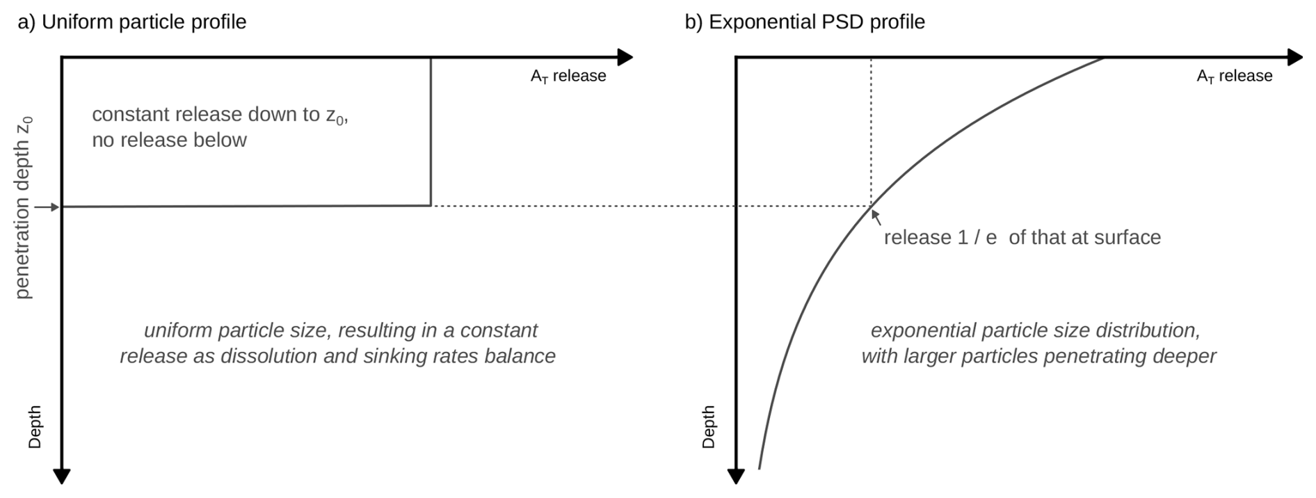
with alkalinity in units mol m⁻³. The factor n_Alk represents the alkalinity release per dissolved mineral molecule (n_Alk=4 for olivine). F denotes the flux of alkalinity stored in the mineral particles entering the ocean (in $\mathrm{mol}{\mathrm{m}}^{-\mathrm{2}}{\mathrm{s}}^{-\mathrm{1}}$), related to the particle flux F_p through $F=F_{\mathrm{p}}\cdot N_{\mathrm{p}}\left(\mathrm{0}\right)\cdot n_{\text{Alk}}$. Similarly as before, the factor n_Alk here translates from the initial number of moles of the mineral in each particle to the corresponding number of moles of alkalinity. Thus, the alkalinity release per unit time is simply given by the mineral alkalinity flux F applied to the surface divided by the penetration depth z₀ for z≤z₀ and vanishing for z>z₀. The alkalinity release profile for uniform particles is depicted in Fig. 1a and validated by an explicit numerical simulation of sinking particles in Appendix Fig. A2.

2.1.3 Alkalinity release profile for an exponential particle size distribution

Now, we consider the case where the mineral particles are not uniform but follow a certain particle size distribution (PSD). To test the effect of particle size dispersion, we here assume an exponential PSD for the distribution of particle number over particle volumes, with the probability density function given by

$$\begin{array}{}\text{(7)}& f\left(V\right)={\displaystyle \frac{\mathrm{1}}{V_{\mathrm{d}}}}{e}^{-V/V_{\mathrm{d}}}.\end{array}$$

The mean particle volume for this PSD is $V_{\mathrm{d}}=\frac{\mathit{\pi }}{\mathrm{6}}{d}^{\mathrm{3}}$ for a given mean volume diameter d. As such, the PSD does not change the average particle volume and alkalinity content relative to uniform particles with the same mean volume diameter d, but adds dispersion around this average volume. As a function of diameter, the PSD is equivalent to a Rosin–Rammler (or identically Weibull) distribution with shape 3 and scale given by the mean volume diameter d (shown in Appendix Fig. A1a).

The Rosin–Rammler distribution is a common model for mineral particle size distributions (e.g., Jillavenkatesa et al., 2001). The shape parameter of 3 indicates a light-tailed distribution. The distribution of particle mass for this PSD is a generalized gamma distribution with shape parameters 3 and 6 and scale d (Appendix Fig. A1b), obtained by weighing the probability density for particle number by particle mass and then normalizing the result to 1. The P80 is the 80th percentile of this mass distribution.

This PSD can now be used to derive the corresponding alkalinity release profile. As discussed before, each particle within the exponential PSD releases the same amount of alkalinity per unit depth. However, smaller particles from the PSD vanish with increasing depth, such that the overall alkalinity release at depth originates from the remaining larger particles, leading to a decrease in alkalinity release with depth.

Equation (5) can be used to determine the minimum initial volume (V_min) for which a particle is still present at depth z. Realizing that $z/V_{\text{min}}=z_{\mathrm{0}}/V_{\mathrm{d}}$, one obtains

$$\begin{array}{}\text{(8)}& V_{\text{min}}\left(z\right)=V_{\mathrm{d}}\cdot {\displaystyle \frac{z}{z_{\mathrm{0}}}}.\end{array}$$

The alkalinity release per unit time at depth z is the product of the remaining incoming particles at depth z and the alkalinity release of each particle:

$$\begin{array}{}\text{(9)}& \begin{array}{rl}{\displaystyle \frac{\mathrm{d}{A}_{\mathrm{T}}}{\mathrm{d}t}}\left(z\right)& =\left(F_{\mathrm{p}}\cdot \underset{V_{\text{min}}\left(z\right)}{\overset{\mathrm{\infty }}{\int }}f\left(V\right)\mathrm{d}V\right)\cdot \left(-{\displaystyle \frac{\mathrm{d}{N}_{\mathrm{p}}}{\mathrm{d}z}}\right)\cdot n_{\text{Alk}}\\ & =\left(F_{\mathrm{p}}\cdot e^{-V_{\text{min}}\left(z\right)/V_{\mathrm{d}}}\right)\cdot \left(-{\displaystyle \frac{\mathrm{d}{N}_{\mathrm{p}}}{\mathrm{d}z}}\right)\cdot n_{\text{Alk}}\\ & ={\displaystyle \frac{F}{z_{\mathrm{0}}}}{e}^{-z/z_{\mathrm{0}}}.\end{array}\end{array}$$

As such, we get an exponentially declining alkalinity release profile when the particle volume is distributed according to an exponential distribution (depicted in Fig. 1b). The exponential decline in alkalinity release is controlled by the penetration depth z₀, the depth at which particles with mean volume diameter d are completely dissolved. The alkalinity release at the surface is equal to that of the uniform particle profile.

2.2 Alkalinity release in the ocean mixed layer

The fraction χ of alkalinity that is released in the mixed layer can be calculated by integrating the alkalinity release profile down to the mixed layer depth (MLD), divided by the total alkalinity release per area and time, F. Here, we use the mean annual maximum mixed layer depth for MLD, representing the frequently ventilated ocean volume. For the uniform particle profile (Eq. 6), the fraction dissolving in the mixed layer is given by

$$\begin{array}{}\text{(10)}& \mathit{\chi }=\left\{\begin{array}{ll}\mathrm{MLD}/z_{\mathrm{0}}& \text{for }\mathrm{MLD}\le z_{\mathrm{0}}\\ \mathrm{1}& \text{for }\mathrm{MLD}>z_{\mathrm{0}}.\end{array}\right.\end{array}$$

Previous studies have calculated the fraction of alkalinity released in the mixed layer based on the decline in particle size during the mixed layer residence time t_MLD in the shrinking core model, $\mathit{\chi }\left(t_{\mathrm{MLD}}\right)=\mathrm{1}-R^{\mathrm{3}}\left(t_{\mathrm{MLD}}\right)/R^{\mathrm{3}}\left(\mathrm{0}\right)$, assuming a constant sinking velocity within the mixed layer such that $t_{\mathrm{MLD}}=\frac{\mathrm{MLD}}{v_{\text{sink}}\left(R\right(\mathrm{0}\left)\right)}$ (Köhler et al., 2013; Renforth and Kruger, 2013; Yang et al., 2025). Our result (Eq. 10) does not require this approximation and is equivalent to computing χ(t_MLD) using the exact residence time obtained from ${\int }_{\mathrm{0}}^{t_{\mathrm{MLD}}}{v}_{\text{sink}}\left(R\right(t\left)\right)\mathrm{d}t=\mathrm{MLD}$ for t_MLD.

For the exponential PSD profile (Eq. 9), integrating the alkalinity release profile down to the MLD and normalizing by F results in

$$\begin{array}{}\text{(11)}& \mathit{\chi }=\mathrm{1}-\exp (-\mathrm{MLD}/z_{\mathrm{0}}).\end{array}$$

2.3 Variation of alkalinity release profiles with environmental conditions

The analytical alkalinity release profiles from Sects. 2.1.2 and 2.1.3 make the assumption of constant environmental conditions throughout particle dissolution. In the ocean, however, temperature and pH typically decrease with depth. A decrease in temperature (T) reduces the area-normalized dissolution rate r (Hangx and Spiers, 2009; Rimstidt et al., 2012), which, to a lesser extent, is countered by an increase in the dissolution rate from the co-occurring decrease in pH. In addition, a reduction in temperature will also increase dynamic viscosity, reducing the particles' sinking velocity. The impact of vertical temperature and pH variations on alkalinity release is further discussed in Sect. 4.2.

To obtain simple analytical alkalinity release profiles, in particular for non-uniform PSDs, we here use local vertically averaged temperature and pH to determine the penetration depths z₀ for the dissolution profiles. However, z₀ depends on the vertical range over which the mean temperature and pH are determined. For example, using average conditions over the upper 100 m will result in higher dissolution rates and a shallower penetration depth z₀ than using average conditions over the upper 1000 m, due to the colder temperatures in the ocean interior. The former would be more appropriate for smaller particles that dissolve close to the surface while the latter would be more appropriate for larger particles. To take into account that larger particles experience colder temperatures (and a often lower pH), we calculate the penetration depth z₀ from Eq. (5) with the mean conditions in temperature and pH between the surface and the penetration depth itself (${\stackrel{\mathrm{‾}}{T}}_{\mathrm{0}\to z_{\mathrm{0}}}$ and ${\stackrel{\mathrm{‾}}{\text{pH}}}_{\mathrm{0}\to z_{\mathrm{0}}}$). In other words, z₀ is calculated self-consistently with mean conditions in temperature and pH over the same vertical range. To do so, we solve

$$\begin{array}{}\text{(12)}& z_{\mathrm{0}}=f\left(r\right({\stackrel{\mathrm{‾}}{T}}_{\mathrm{0}\to z_{\mathrm{0}}},{\stackrel{\mathrm{‾}}{\text{pH}}}_{\mathrm{0}\to z_{\mathrm{0}}}),\mathit{\mu }({\stackrel{\mathrm{‾}}{T}}_{\mathrm{0}\to z_{\mathrm{0}}}\left)\right),\end{array}$$

numerically for z₀. Following this approach, a particle that dissolves close to the surface (small z₀) is modeled to dissolve under a warmer average temperature than a particle that penetrates the colder deep ocean (large z₀).

2.4 Experimental design with GFDL ESM2M

In this study, we use the Earth system model GFDL ESM2M to determine OAE efficiency for the here developed alkalinity release profiles. GFDL ESM2M (Dunne et al., 2012, 2013) is a fully coupled carbon-climate Earth system model from NOAA GFDL, which contributed to the Coupled Model Intercomparison Project phase 5 (CMIP5). Its ocean component MOM4p1 (Griffies, 2009) uses a horizontal grid with 1° nominal resolution and 50 vertical layers with 10 m vertical resolution in the upper ocean. Ocean biogeochemistry is simulated by the Tracers of Ocean Phytoplankton with Allometric Zooplankton version two (TOPAZv2 Dunne et al., 2013), and carbonate chemistry follows the OCMIP2 recommendations (Najjar and Orr, 1998) with air-sea CO₂ exchange determined by the bulk parameterization by Wanninkhof (1992).

As a first step, the penetration depth parameter z₀ is calculated for forsterite (the most common form of olivine) for three different diameters, d = 1.72 µm, d = 2.58 µm, and d = 3.44 µm (hereafter rounded to 1.7, 2.6, and 3.4 µm for better readability), with environmental conditions from GFDL ESM2M. The three diameters were selected to show the transition from shallow to deep particle penetration depth. z₀ is calculated for each vertical column of the ocean model grid separately, based on temporally averaged temperature and pH profiles over the period 2016–2025 and for five initial-condition ensemble members (50 years in total). The period 2016–2025, extending an emission-driven historical simulation (Lacroix et al., 2024), is forced with Global Carbon Budget CO₂ emissions over 2016–2020 extended with NDCs for 2021–2025 (Friedlingstein et al., 2020), and non-CO₂ forcing as well as land use changes prescribed from RCP2.6 (Van Vuuren et al., 2011). Since z₀ is determined in a fixed time-period, the impact of climate change on the dissolution profiles is not considered here. We take the area-normalized dissolution rate of forsterite for geometric surfaces as a function of temperature and pH from Rimstidt et al. (2012), also validated in Oelkers et al. (2018) and Fuhr et al. (2022) (see Appendix Fig. A3). Dynamic seawater viscosity as a function of temperature is interpolated from the tabulated data in The Engineering ToolBox (2005). Forsterite density is taken from Anthony et al. (2001) and seawater density is set to global surface ocean conditions of T = 18 °C and S = 35 PSU (The Engineering ToolBox, 2005). Variations in seawater density are negligible for particle sinking velocity since they are small compared to the density difference between the mineral particles and seawater. Alkalinity release that is prescribed below the ocean bottom cell is added to the bottom cell.

Based on the spatially-varying penetration depths for the three diameters and the two alkalinity release profile types (uniform particles and exponential PSD), we run six OAE experiments with differing alkalinity release profiles in GFDL ESM2M. Following the CDRMIP protocol, alkalinity is continuously added to the global ocean between 60° S and 70° N, totaling to 0.14 Pmol alkalinity per year (Keller et al., 2018). For each of the six OAE experiments, GFDL ESM2M is run over the period 2026–2200, under a CO₂ emission trajectory that stabilizes at 2 °C global warming relative to the preindustrial period in absence of OAE (based on the AERA protocol; Terhaar et al., 2022; Silvy et al., 2024). These six simulations are compared to a simulation where alkalinity is added at the ocean surface. For the uniform alkalinity release profiles with d = 2.6 µm and d = 3.4 µm and for surface alkalinity addition, we ran four additional ensemble members for the period 2026–2035 to analyze the role of internal variability over the first 10 years of OAE. All simulations are run with interactive atmospheric CO₂ rather than prescribed concentrations. Thus, the OAE efficiency; calculated as the difference in air-sea carbon uptake between the OAE experiment and the baseline simulation without OAE divided by the alkalinity addition; includes carbon cycle feedbacks between the ocean, atmosphere, and land biosphere. This net ocean capture efficiency including the carbon cycle feedbacks is lower than the gross efficiency, which is calculated without the adjustments in natural carbon reservoirs (Grosselindemann et al., 2026). The net efficiency is relevant for studying the carbon, climate and ocean acidification responses to OAE, while the gross efficiency characterizes the negative emissions due to OAE, thus important for emission budgets and carbon credits.

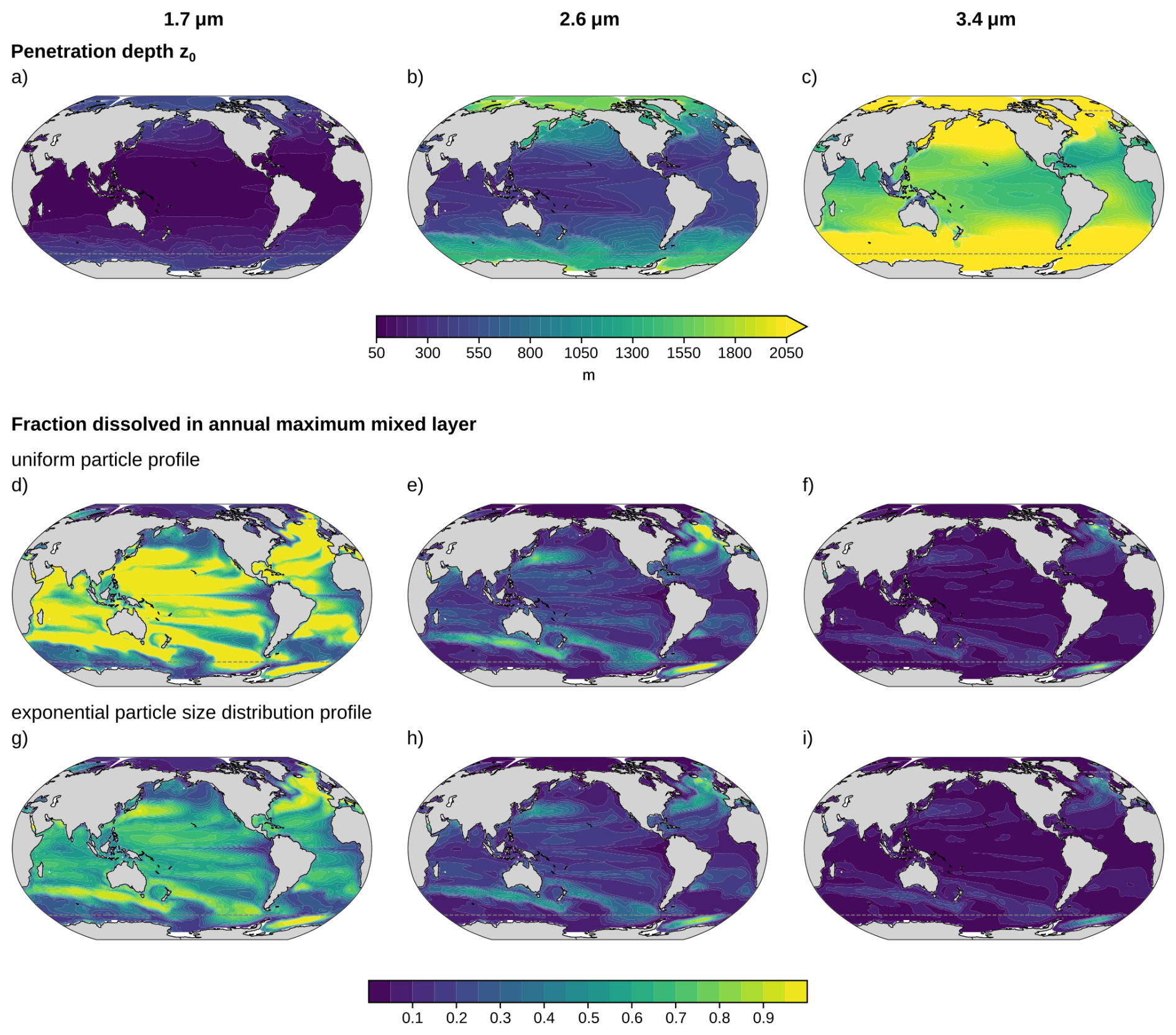
Figure 2 Regional variation in penetration depth and mixed layer alkalinity release for particle diameters d = 1.7 µm (left column), d = 2.6 µm (middle column), and d = 3.4 µm (right column). (a–c) Penetration depth determined with temperature and pH data from GFDL ESM2M over the period 2016–2025 (see Sects. 2.3 and 2.4). The fraction of alkalinity released above the annual maximum mixed layer depth (χ) for uniform particle profiles are shown in panels (d–f) and those for exponential particle size distribution profiles in panels (g-i) for each penetration depth. The gray dashed lines enclose the region between 60° S and 70° N, where alkaline minerals are added to the surface ocean in this study.

3 Results

3.1 Regional variation in alkalinity release

The penetration depth z₀, calculated from Eqs. (5) and (12), increases strongly with particle size (Fig. 2a–c). Globally averaged, z₀ values are 165 m, 638 m, and 1945 m for particle diameters of d = 1.7 µm, d = 2.6 µm, and d = 3.4 µm, respectively. Thus, doubling the diameter from d = 1.7 µm to d = 3.4 µm increases z₀ by about a factor of twelve. Under constant environmental conditions, Eq. (5) predicts a scaling of z₀∝d³, corresponding to an eightfold increase. The stronger increase in z₀ arises from overall cooler conditions experienced by larger particles that sink deeper into the water column as discussed in Sect. 2.3.

The penetration depth shows a pronounced latitudinal gradient (Fig. 2a–c). It is substantially greater at high latitudes than at low latitudes. For example, for d = 2.6 µm, the average penetration depth increases from 367 m in the tropics (10° S–10° N) to 1043 m in the Southern Ocean (60 to 45° S). This pattern arises primarily from lower water temperatures in high latitude regions, which suppress mineral dissolution rates and thereby increase penetration depth. The effect of reduced dissolution is partially counteracted by the higher viscosity of colder waters, which slows particle sinking and limits penetration. However, the change in dissolution rate with temperature dominates: a 1 °C cooling at 18 °C results in a 9.2 % decrease in area-normalized dissolution rate, whereas viscosity only increases by 2.6 %. Latitudinal variations in pH exert a negligible impact on mineral dissolution rate (Appendix Fig. A3). Even variations in pH of ± 0.1 alter z₀ by only a few meters.

Based on these penetration depths, the fraction of alkalinity released within the annual maximum mixed layer can be calculated (Sect. 2.2, Fig. 2d–i). Because waters above the annual maximum MLD are well ventilated, alkalinity released in this layer directly contributes to oceanic carbon uptake. The fraction of alkalinity released in the mixed layer decreases with increasing particle size and is larger for the uniform particle profile than for the exponential profile, as larger particles in the latter are exported to greater depths. Globally, uniform particles with d = 1.7 µm release 72 % of their alkalinity within the annual maximum mixed layer (Fig. 2d), compared to 52 % for the exponential PSD profile with the same mean volume diameter (Fig. 2g). Increasing the (mean volume) diameter to d = 2.6 µm lowers the fraction to 20 % and 18 % for the uniform and exponential profile, respectively, and further to 6 % for both profiles at d = 3.4 µm. For large diameters, the penetration depth is often much larger than the mixed layer depth and the alkalinity release within the mixed layer between profiles is similar, because: $\mathrm{1}-\exp (-\mathrm{MLD}/z_{\mathrm{0}})\approx \mathrm{MLD}/z_{\mathrm{0}}$ for $\mathrm{MLD}/z_{\mathrm{0}}\ll \mathrm{1}$.

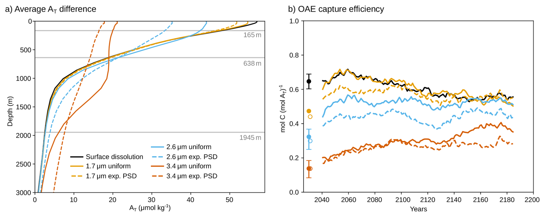
Figure 3 (a) Global mean difference in total alkalinity between the OAE simulations (surface dissolution and uniform as well as exponentially distributed particle size distributions) and the baseline simulation without OAE, averaged over 2026–2200. The horizontal gray lines indicate the global mean penetration depths z₀ for the three particle diameters 1.7, 2.6, and 3.4 µm. (b) The OAE efficiency for these simulations over time, defined as the number of moles of additional carbon uptake in the OAE simulations divided by the number of moles alkalinity added. The lines show 31 year running means. The dots indicate averages over the first 10 years of the experiment, with open dots for the PSD experiments. For surface dissolution and the 2.6 and 3.4 µm uniform cases, the five-member ensemble ranges and ensemble means shown.

Regionally, alkalinity release in the mixed layer is large either where penetration depths are shallow (low to mid-latitudes; Fig. 2a–c) or where mixed layers are deep (e.g., western boundary current extension in the North Atlantic and North Pacific, the mode water formation regions of the Southern Ocean, and deep convection zones in the North Atlantic and Weddell Sea; Appendix Fig. A4). Since regions are often either warm, associated with shallow penetration depths, or have deep mixed layers, the latitudinal gradients of alkalinity release in the mixed layer are relatively small. For example, uniform particles with d = 2.6 µm release 14 % of their alkalinity in the mixed layer in the tropics (10° S–10° N) and 20 % in the Southern Ocean (60 to 45° S).

3.2 Ocean carbon uptake and efficiency

Each profile type (uniform and exponential PSD) and particle size results in a characteristic vertical distribution of additional alkalinity relative to the reference simulation without OAE (Fig. 3a, Appendix Fig. A5). Averaged over 2026–2200, the additional alkalinity profile of the smallest mean volume diameter d = 1.7 µm closely resembles that from surface dissolution, with only slightly lower concentrations close to the surface (57 µmol kg⁻¹ for surface dissolution vs. 55 and 52 µmol kg⁻¹ for the uniform and exponential PSD profiles, respectively). With increasing particle diameter, additional alkalinity accumulates at larger depths. This is particularly the case for the exponential PSD profile, where 37 % of the alkalinity is released below z₀ compared to no release below z₀ for the uniform profile (global mean values for z₀ are shown as dashed lines in Fig. 3a). As a result, additional alkalinity near the surface declines. For d = 3.4 µm, additional surface alkalinity reduces to 21 and 18 µmol kg⁻¹ for the uniform and exponential PSD profiles, respectively.

Relative to surface alkalinity release, this deeper alkalinity release reduces OAE capture efficiency, defined as the ratio of additional carbon uptake to the alkalinity added (Fig. 3b). The reduction is most pronounced in the first decades of continuous alkalinity addition. Over the first 30 years, efficiency decreases by more than two thirds for d = 3.4 µm, to 0.20 and 0.18 mol C_T (mol A_T)⁻¹ for the uniform and exponential PSD profiles, respectively, compared to 0.65 mol C_T (mol A_T)⁻¹ for surface dissolution and alkalinity release. For reference, an efficiency of 0.65 mol C_T (mol A_T)⁻¹ corresponds to an uptake of 0.81 Gt CO₂ per Gt forsterite. For the intermediate mean volume diameter d = 2.6 µm, efficiency is reduced to 0.44 mol C_T (mol A_T)⁻¹ (−32 %) and 0.39 mol C_T (mol A_T)⁻¹(−40 %) for the uniform and exponential PSD profiles, respectively. For the exponential PSD profile with the smallest mean volume diameter d = 1.7 µm, we find a 16 % decrease in efficiency to 0.54 mol C_T (mol A_T)⁻¹. Efficiency is further reduced during the first decade with 0.32 and 0.14 mol C_T (mol A_T)⁻¹ for uniform particles with d = 2.6 and 3.4 µm, respectively, compared to 0.65 mol C_T (mol A_T)⁻¹ for surface dissolution (on ensemble mean, ensemble ranges are shown in Fig. 3b). As such, efficiency decreases by more than 75 % over the first 10 years for particles with 3.4 µm diameter. We also find a reduced efficiency of 0.47 mol C_T (mol A_T)⁻¹ (−27 %) for uniform particles with d = 1.7 µm during the first decade.

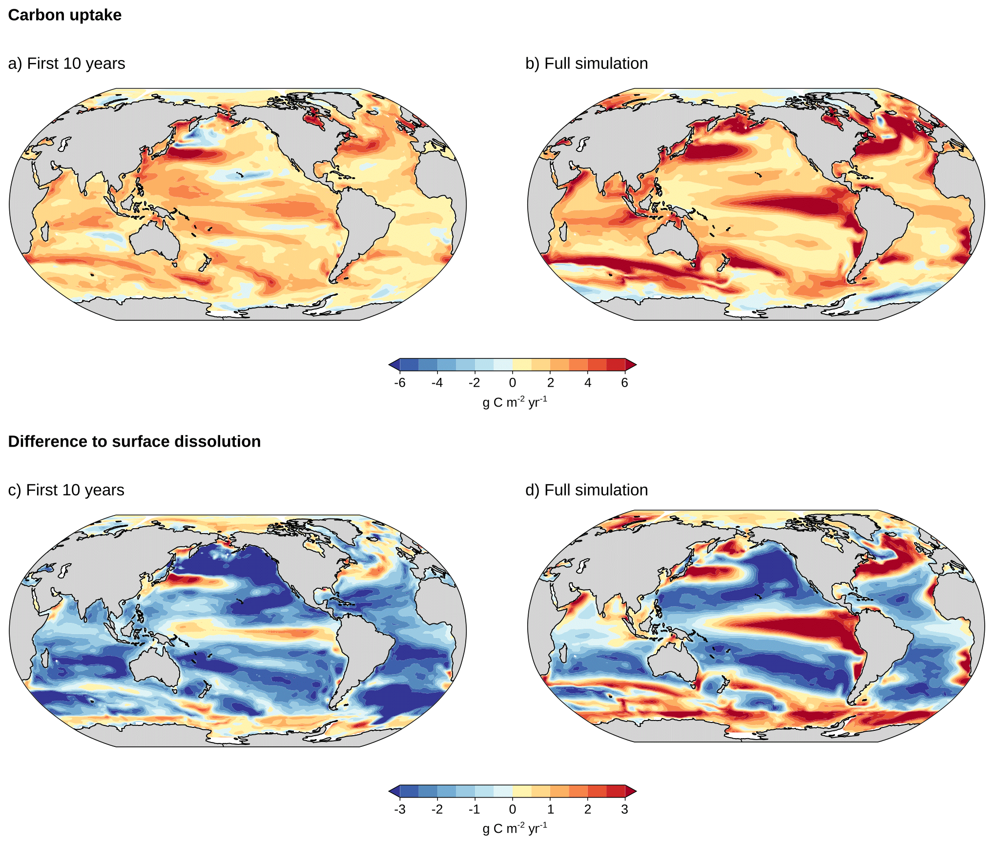
Figure 4 Regional carbon uptake for the OAE experiment with uniform particles of diameter d = 2.6 µm relative to the baseline simulation without ocean alkalinity enhancement over (a) the first 10 years (2026–2035), averaged over five ensemble members to increase robustness, and (b) over the full simulation (2026–2200). The difference between the carbon uptake for this uniform particle size and that for surface alkalinity addition is shown in panels (c) for the first 10 years and (d) for the full period.

Over time, the difference in efficiency relative to surface alkalinity release decreases, reflecting the gradual transport of alkalinity released at depth back to the surface. Nevertheless, the average efficiency over 2026–2200 remains less than half of that of surface addition for d = 3.4 µm (0.29 and 0.25 mol C_T (mol A_T)⁻¹, respectively, compared to 0.60 mol C_T (mol A_T)⁻¹). Year-to-year variability in OAE efficiency is substantial in all experiments (standard deviation around 0.18 mol C_T (mol A_T)⁻¹). These strong fluctuations in carbon uptake mainly arise because we run the experiments in a fully coupled Earth system model, where natural variations in air-sea CO₂ flux in the OAE experiment and the baseline simulation are superimposed onto the carbon uptake signal from OAE. For larger particle sizes, the standard deviation of OAE efficiency approaches mean efficiency (coefficients of variation are 0.56 and 0.72 for the uniform and exponential PSD profiles with d = 3.4 µm). Thus, the OAE carbon uptake signal is less significant compared to flux variability when alkalinity is released from larger particles.

During the first 10 years of alkalinity addition, OAE with vertical alkalinity release profiles results in additional carbon uptake over most of the ocean (see Fig. 4a for the additional CO₂ uptake for uniform particles with diameter d = 2.6 µm). However, carbon uptake and efficiency are generally lower than when alkalinity is released directly at the surface (Fig. 4c). As expected, regions with particularly low alkalinity release in the mixed layer (Fig. 2e) partially overlap with regions of low carbon uptake (Fig. 4a), such as in the northern and eastern North Pacific or the Atlantic section of the Southern Ocean. Carbon uptake is higher in the Kuroshio current extension, the Gulf Stream region in the North Atlantic, and mode water source regions in the Southern Ocean, where the fraction of alkalinity release in the mixed layer is also relatively high. However, despite relatively low alkalinity release in the mixed layer, the tropical upwelling regions show considerable carbon uptake, which may indicate the upwelling of alkalinity back to the surface. Overall, the fraction of alkalinity release in the annual maximum mixed layer only partially explains the regional variations in carbon uptake even on short timescales such as 10 years. The pattern correlation between the fraction of alkalinity release in the mixed layer and OAE-induced carbon uptake for d = 2.6 µm particles, averaged over the 5 ensemble members, is only 0.34 between 60° S and 70° N. However, the carbon uptake pattern also varies strongly among the five ensemble members. We analyze this by calculating the pattern correlation coefficients between the carbon uptake patterns of the different ensemble members over the first 10 years of experiment. The mean of the ten pairwise pattern correlation coefficients across the five ensemble members is 0.15 and 0.37 for uniform d = 3.4 µm and d = 2.6 µm particles, respectively. As such, regional carbon uptake is more uncertain for larger particles where alkalinity is released deeper in the water column.

At longer timescales, ocean carbon uptake increases in regions with deep mixed layers (cf. Fig. 4b and Appendix Fig. A4), in the upwelling region of the tropical Pacific, as well as in Eastern Boundary upwelling systems (Fig. 4b). The increase in carbon uptake in these regions suggests that additional alkalinity released at subsurface in other regions is transported there, where it comes in contact with the atmosphere. In the eastern and central equatorial Pacific, for example, we find a distinct buildup of alkalinity in the upper 1000 m, likely due to an inflow of alkalinity from North and South of the equator (Appendix Fig. A5f). As these waters with additional alkalinity have not yet equilibrated with the atmosphere, additional carbon is taken up. As a result, carbon uptake becomes larger than in the simulation with direct alkalinity addition at the surface in these regions (Fig. 4d). Increased carbon uptake is also observed south of 60° S where no alkalinity is added, indicating an increased southward transport of alkalinity from regions north of 60° S when alkalinity is released at subsurface. Yet, carbon uptake remains lower over most of the low-to-mid latitudes, such that global carbon uptake remains 16 % lower than when alkalinity is added to the surface (Fig. 3b).

4 Discussion

4.1 Comparison to earlier studies

Our study suggests a shallower release of alkalinity compared to Köhler et al. (2013), who estimated that about 80 % of alkalinity from forsterite olivine particles with a 1 µm diameter is released within the maximum mixed layer. Repeating the analysis from Sect. 3.1 for particles of 1 µm diameter, we find a release of 98 % in the annual maximum mixed layer. The shallower release of alkalinity in our study primarily arises from the higher area-normalized dissolution rate adopted here, based on geometric surfaces from Rimstidt et al. (2012). For example, the dissolution rate is 84 % higher at 25  °C than the rate from Hangx and Spiers (2009) used in Köhler et al. (2013). A secondary contribution stems from the deeper maximum MLD in our model, 123 m on global average (34 m deeper than observations; Dunne et al., 2012), compared to 64 m in Köhler et al. (2013). As the dissolution rate from Rimstidt et al. (2012) has been validated against observations in multiple studies (Oelkers et al., 2018), the mixed layer alkalinity release fractions obtained here are likely more robust. Nonetheless, the comparison underscores the strong sensitivity of vertical alkalinity release to the assumed mineral dissolution rate. Despite the shallower release, the spatial patterns of mixed layer alkalinity release are broadly consistent with those of Köhler et al. (2013) (cf. Fig. 2 and their Fig. 3d).

Our results are also qualitatively consistent with Fakhraee et al. (2023), who modeled alkalinity release using a more complex mineral particle model that includes particle aggregation and zooplankton interaction. Their study employed an experimental PSD from Renforth (2012), in which 80 % of particle mass is contained in particles smaller than 10 µm in diameter. To enable comparison, we discretize the experimental PSD into 14 discrete size classes and convert the experimentally determined mass fractions per size class into particle number fractions (see Appendix Sect. A and Fig. A7a). The resulting cumulative alkalinity release profiles (Fig. A7b) are qualitatively similar to those reported by Fakhraee et al. (2023) though our model predicts a shallower release. While Fakhraee et al. (2023) found 25 % to 45 % of alkalinity release in the upper 80 m, with increased release for higher feedstock application rates where aggregates are less likely packed into zooplankton fecal pellets, we obtain 54 % to 61 % for temperatures of 10 to 25 °C. This difference suggests that including particle aggregation and zooplankton ingestion, as in Fakhraee et al. (2023), may further reduce the efficiency of olivine-based ocean alkalinity enhancement by enhancing particle settling velocities.

4.2 Limitations of the analytical shrinking core treatment of mineral particles

The analytical framework presented here involves several simplifying assumptions. The main limitations include (i) the idealized representation of particle geometry and sinking, (ii) the omission of particle interactions with the environment such as aggregation, scavenging, or the formation of coating layers, (iii) the use of mean rather than depth-resolved environmental conditions, and (iv) the omission of particle advection during dissolution.

First, the shrinking core model assumes smooth, spherical particles. We use an area-normalized dissolution rate determined for geometric spherical particles with equivalent diameters determined by sieving the mineral grains (Rimstidt et al., 2012). The particles' sinking velocity, on the other hand, is characterized by the equivalent diameter from Stokes settling. While the two equivalent diameters are often similar (Wills and Finch, 2016), implying that the treatment of dissolution and sinking in our study is consistent, this may not always be the case. When the two equivalent diameters diverge, one cannot assign a single equivalent spherical diameter to a mineral particle that is representative for both dissolution and sinking as assumed in our alkalinity release profiles. Additionally, when mineral particles are added over a small area such that high mineral particle concentrations near 15 g L⁻¹ are reached, fluid instabilities may considerably enhance the sinking velocity (Yang and Timmermans, 2024; Yang et al., 2025). While such mineral particle concentrations in the mixed layer are not reached in our idealized global experiments, where only 15 g olivine per square meter and year are added, instabilities may occur in more realistic localized application schemes.

Second, we also neglect potential particle interactions with the environment. Smaller mineral particles may aggregate, forming larger particles that sink faster (Köhler et al., 2013). Mineral particles may also attach to biogenic particles through scavenging or zooplankton ingestion, suppressing near-surface alkalinity release (Fakhraee et al., 2023). Mineral or microbial coating layers may form on the particles' surfaces (Wang and Giammar, 2013; Oelkers et al., 2018), which can reduce the contact area with the surrounding water and mineral dissolution.

Third, to obtain analytical alkalinity release profiles, we assume that dissolution occurs at the mean temperature and pH between surface and penetration depth z₀ (Sect. 2.3). This simplification neglects vertical and seasonal gradients that could enhance dissolution in warmer surface waters and reduce it at depth. The approximation performs best where such gradients are small (e.g., at high latitudes or for shallow-sinking particles). For instance, in a subtropical Atlantic column with a 9.2 °C temperature range between surface and a particle's penetration depth of 300 m, surface alkalinity release is 27 % higher and deep release is 28 % lower than predicted using mean conditions, whereas in the Southern Ocean (1.8 °C range) the differences are only 9 % and 2 %, respectively (Fig. A6a,b). The stronger mismatch at low latitudes thus reflects the larger vertical temperature contrast. The use of mean environmental conditions to determine a particle’s penetration depth also neglects the nonlinear dependence of dissolution rate on temperature and pH (Rimstidt et al., 2012). Because the dissolution rate is a convex function of these variables, the rate at vertically averaged conditions is slightly lower than the average rate computed over the full profile, resulting in a deeper predicted penetration depth. This effect is generally small: across the global ocean, penetration depths differ by less than 10 % over 90 % of the area for 2.6 µm particles (Fig. A6d). For these particles, explicit profiles yield a globally averaged penetration depth that is only 14 m shallower than the idealized case, though mixed-layer release fractions increase by about 6 % (a relative rise of 28 %, Fig. A6f). Hence, while vertically resolved profiles yield higher surface release, the idealized treatment remains a good first-order approximation. For the exponential PSD profile, we also assume that all particle sizes experience identical mean temperature and pH, although larger particles typically penetrate into colder, more acidic waters than smaller ones. Accounting for these variations would increase the spread in penetration depth across the PSD, resulting in a deeper alkalinity export for larger particles.

Fourth, the present framework neglects the horizontal and vertical advection of mineral particles during dissolution. Because dissolution can span several years (Appendix Fig. A2a), advection of mineral particles in the subsurface may modify the depth and spatial patterns of alkalinity release. This aspect should be assessed in subsequent studies.

Overall, these simplifications may lead to a modest underestimation of mineral export and deep alkalinity release, primarily due to the omission of particle aggregation. Nevertheless, the simplified vertical profiles developed here capture the first-order effects of environmental conditions and feedstock properties on alkalinity release, providing a robust basis for sensitivity analyses of ocean alkalinity enhancement efficiency.

4.3 Implications for feasibility of open-ocean mineral-based OAE

Our study confirms that olivine must be milled to grain sizes near 1 µm to achieve feasible carbon removal through open-ocean alkalinity enhancement (Köhler et al., 2013; Boyd and Vivian, 2019). When particles are uniformly milled to a diameter of 1.7 µm, carbon capture efficiency is reduced over the first decade but comparable to that of instantaneous surface dissolution on longer timescales. In contrast, doubling the diameter to 3.4 µm reduces the efficiency to less than one third within the first decades.

Olivine powder with an exponential PSD at a mean volume diameter of 1.7 µm marks a transition between near-optimal and considerably reduced capture efficiency. In this case, efficiency is 16 % lower than with direct surface alkalinity addition over the first 3 decades, with full efficiency reached only by the end of the 21st century (Fig. 3b). These long timescales until full efficiency result from an overproportionally larger fraction of alkalinity stored in the larger particles that sink deeper. While 80 % of particles are smaller than 2 µm, they only contain 48 % of the alkalinity. In contrast, the largest 0.3 % of particles in the PSD, exceeding 3.1 µm, still contain 2 % of the alkalinity. In natural or industrially milled powders, more heavy-tailed PSDs can further exacerbate this problem. For example, in the experimental PSD from Renforth (2012), 73 % of the alkalinity resides in the largest 0.3 % of particles, resembling a power law distribution (Fig. A7a). For this heavy-tailed PSD, 20 % of the alkalinity is contained in particles with diameters larger than 10 µm, compared to only 2.5 µm for the exponential PSD, despite a smaller mean particle volume in the experimental PSD. Thus, beyond minimizing mean volume diameter, achieving a rapid decay of particle abundance at larger sizes is essential for efficient OAE. As such, separating and regrinding the largest particles in the mineral powder would, if possible, improve OAE efficiency.

The strong dependence of carbon capture efficiency on the particle size distribution makes particle comminution to grain sizes near 1 µm for olivine-based open-ocean OAE imperative. However, grinding olivine to such fine grain sizes strongly increases energy demand and associated costs and emissions. Foteinis et al. (2023) estimated CO₂ emissions to increase from 0.04 t CO₂ (1.25 t olivine)⁻¹ for 10 µm particles to about 0.21 t CO₂ (1.25 t olivine)⁻¹ for 1 µm particles from comminution alone, translating to reductions in OAE capture efficiency by 0.03 and 0.13 mol C (mol A_T)⁻¹, respectively. Additionally, such fine olivine powders may increase particle aggregation (Köhler et al., 2013), negatively impact zooplankton (Fakhraee et al., 2023), and pose risks to human health (Doelman et al., 1990). These problems with olivine grain sizes near 1 µm call into question the feasibility of olivine-based OAE in the open ocean. However, olivine may remain suitable for coastal applications where the mixed layer extends to the seafloor, such that alkalinity released from coarser olivine grains in the sediments enhances carbon uptake from the atmosphere (Renforth, 2012; Montserrat et al., 2017; Foteinis et al., 2023). Future research should therefore focus on shallow coastal seas. The micrometer scale olivine grain size necessary for open-ocean OAE and associated high particle amounts may also impact marine ecosystems due to increases in turbidity. While no detrimental impacts were observed for coastal plankton communities with coarser olivine powder (Guo et al., 2024), turbidity-associated impacts on plankton should be investigated with micrometer-scale olivine powder, and ideally also for open-ocean ecosystems.

Alternative alkaline materials with higher dissolution rates, such as brucite, relax the particle-size constraints. Using Eq. (5), one can calculate the permissible increase in particle volume for a more quickly dissolving material (indicated by primes) such that the penetration depth stays constant:

$$\begin{array}{}\text{(13)}& {\displaystyle \frac{V_{\mathrm{d}}^{\prime }}{V_{\mathrm{d}}}}={\displaystyle \frac{r^{\prime }}{r}}\cdot {\displaystyle \frac{V_{\text{mol}}^{\prime }}{V_{\text{mol}}}}\cdot {\displaystyle \frac{{\mathit{\rho }}_{\mathrm{p}}-{\mathit{\rho }}_{\mathrm{w}}}{{\mathit{\rho }}_{\mathrm{p}}^{\prime }-{\mathit{\rho }}_{\mathrm{w}}}}\end{array}$$

Because brucite dissolves roughly 100 times faster than forsterite at T = 25 °C and pH = 8 (Pokrovsky and Schott, 2004), the allowable particle volume increases by a factor of 90, corresponding to an increase in diameter by a factor of 4.5. Thus, an exponential PSD with mean volume diameter of 1.7 µm for forsterite corresponds to an equally efficient PSD with mean volume diameter of 7.7 µm for brucite. Importantly, dissolution rates of brucite have been shown to vary by orders of magnitude depending on crystalline structure (Shaw et al., 2025), making particle size constraints for effective brucite-based OAE in the open ocean uncertain.

The framework developed here can be generalized to other PSDs by deriving corresponding vertical alkalinity release profiles, as illustrated for the exponential and discrete PSDs. This approach provides a direct estimate of the alkalinity released within the mixed layer (Sect. 2.2), improving on earlier approaches assuming constant sinking velocity in the mixed layer (Renforth and Kruger, 2013; Köhler et al., 2013; Yang et al., 2025). Our Earth system model simulations indicate, however, that regional variation in oceanic carbon uptake is only partly explained by mixed-layer dissolution. The remaining differences highlight the role of ocean circulation and alkalinity redistribution, which can only be captured with ocean-biogeochemical models.

Such ocean-biogeochemical models are also essential for assessing how mineral OAE with subsurface alkalinity release affects ocean acidification (OA). Relative to surface dissolution, and averaged over 2026–2200, mineral OAE with an exponential PSD at a mean volume diameter of 3.4 µm results in a 0.015 unit lower pH (weaker OA mitigation) in the upper 482 m of the water column, and a 0.015 unit higher pH (stronger OA mitigation) at greater depths (Appendix Fig. A8c). Notably, OA mitigation is increased below 482 m even though the alkalinity enhancement is smaller than under surface dissolution down to 792 m (Fig. 3a). This occurs because waters contain lower dissolved inorganic carbon concentrations as a result of the lower ocean carbon uptake under subsurface alkalinity addition. Overall, these results indicate a downward shift in the depth of OA mitigation and an enhanced mitigation potential driven by the reduced carbon uptake and efficiency of the mineral-based OAE.

5 Conclusions

In summary, the efficiency of mineral-based alkalinity enhancement in the open ocean and associated CO₂ uptake is highly sensitive to feedstock particle-size characteristics. Insufficient comminution can substantially reduce carbon capture efficiency and delay CO₂ uptake by decades to centuries, often shifting it far away from the deployment site. Such temporal and spatial lags complicate monitoring, reporting and verification and challenge carbon crediting schemes based on short-term removal. For olivine, required grain sizes of around 1.7 µm likely render its application in the open ocean unfeasible. More rapidly dissolving minerals may prove to be suitable for efficient alkalinity enhancement when mineral particle properties are closely controlled. Our findings emphasize the need for integrated process–energy–climate assessments to evaluate the feasibility of mineral-based alkalinity enhancement in the open ocean.

Appendix A: Alkalinity release for the experimental PSD by Renforth (2012)

To derive an alkalinity release profile, we first discretize the particle size distribution from Table 1 in Renforth (2012) by assuming all particles within the 14 particle size intervals to have the respective mean diameters of the intervals $d_{i=\mathrm{1},\mathrm{\dots }\mathrm{14}}$. We then calculate the particle volume for each size class as $V_i=\frac{\mathit{\pi }{d}_i^{\mathrm{3}}}{\mathrm{6}}$. As a next step, the retained mass fractions m_i in each interval are transformed into number fractions n_i. The number of particles in size class i is given by $V_{\text{tot}}\cdot m_i/V_i$, with the total volume of all particles V_tot and that in size class i given by V_tot⋅m_i when assuming constant density. The number fraction in size class i then follows as

$$n_i={\displaystyle \frac{V_{\text{tot}}\cdot m_i/V_i}{{\sum }_i{V}_{\text{tot}}\cdot m_i/V_i}}={\displaystyle \frac{m_i/V_i}{{\sum }_i{m}_i/V_i}}.$$

The probability density function for these discrete number fractions n_i at volumes V_i is then given by

$$f\left(V\right)=\sum _i{n}_i\cdot \mathit{\delta }(V-V_i).$$

The mean particle volume of the distribution is calculated as $\stackrel{\mathrm{‾}}{V}={\sum }_i{n}_i{V}_i$. The penetration depth z₀, the depth at which particles with mean volume $\stackrel{\mathrm{‾}}{V}$ are completely dissolved, is calculated according to Eq. (5). The alkalinity release profile can now be calculated as done for the exponential PSD in Eq. (9):

$$\begin{array}{rl}{\displaystyle \frac{\mathrm{d}{A}_{\mathrm{T}}}{\mathrm{d}t}}\left(z\right)& =\left(F_{\mathrm{p}}\cdot \underset{V_{\text{min}}\left(z\right)}{\overset{\mathrm{\infty }}{\int }}f\left(V\right)\mathrm{d}V\right)\cdot \left(-{\displaystyle \frac{\mathrm{d}{N}_{\mathrm{p}}}{\mathrm{d}z}}\right)\cdot n_{\text{Alk}}\\ & =F_{\mathrm{p}}\left(-{\displaystyle \frac{\mathrm{d}{N}_{\mathrm{p}}}{\mathrm{d}z}}\right)\cdot n_{\text{Alk}}\cdot \sum _i{n}_i\underset{V_{\text{min}}\left(z\right)}{\overset{\mathrm{\infty }}{\int }}\mathit{\delta }(V-V_i)\mathrm{d}V\\ & =F_{\mathrm{p}}\left(-{\displaystyle \frac{\mathrm{d}{N}_{\mathrm{p}}}{\mathrm{d}z}}\right)\cdot n_{\text{Alk}}\cdot \sum _i{n}_i\mathit{\theta }(V_i-V_{\text{min}}(z\left)\right)\\ & ={\displaystyle \frac{F}{z_{\mathrm{0}}}}\sum _i{n}_i\mathit{\theta }(V_i-V_{\text{min}}(z\left)\right),\end{array}$$

with θ representing the Heavyside step function (θ(x)=0 for x<0 and 1 else) and V_min(z) the minimum initial volume of a particle to still be present at depth z (Eq. 8).

Finally, the fraction of alkalinity release between the surface and depth z is calculated by integrating the alkalinity release profile and normalizing by the surface alkalinity flux (see Sect. 2.2):

$$\begin{array}{rl}{\displaystyle \frac{\mathrm{1}}{F}}\underset{\mathrm{0}}{\overset{z}{\int }}{\displaystyle \frac{\mathrm{d}{A}_{\mathrm{T}}}{\mathrm{d}t}}\left(z\right)\mathrm{d}z& ={\displaystyle \frac{\mathrm{1}}{z_{\mathrm{0}}}}\sum _i{n}_i\underset{\mathrm{0}}{\overset{z}{\int }}\mathit{\theta }(V_i-V_{\text{min}}(z\left)\right)\mathrm{d}z\\ & ={\displaystyle \frac{\mathrm{1}}{z_{\mathrm{0}}}}\sum _i{n}_i\cdot \text{min}(z,z_{\mathrm{0}}{\displaystyle \frac{V_i}{\stackrel{\mathrm{‾}}{V}}}).\end{array}$$

In the last step, it was used that θ(V_i−V_min(z)) is zero if V_i<V_min(z), which is the case if $z>z_{\mathrm{0}}\frac{V_i}{\stackrel{\mathrm{‾}}{V}}$ (Eq. 8).

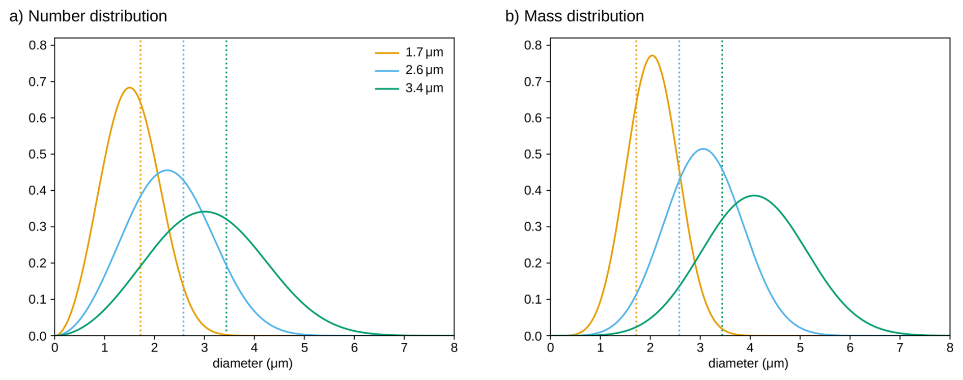
Figure A1 Probability density functions as a function of particle diameter for the exponential PSDs analyzed in this study. Panel (a) shows the distribution of particle number across diameters (a Rosin–Rammler distribution with shape 3 and scale given by the mean volume diameter d) and panel (b) displays the distribution of particle mass (a generalized gamma distribution with shape parameters p=3 and d=6 and scale d). Vertical dotted lines display the mean volume diameters d of the three distributions.

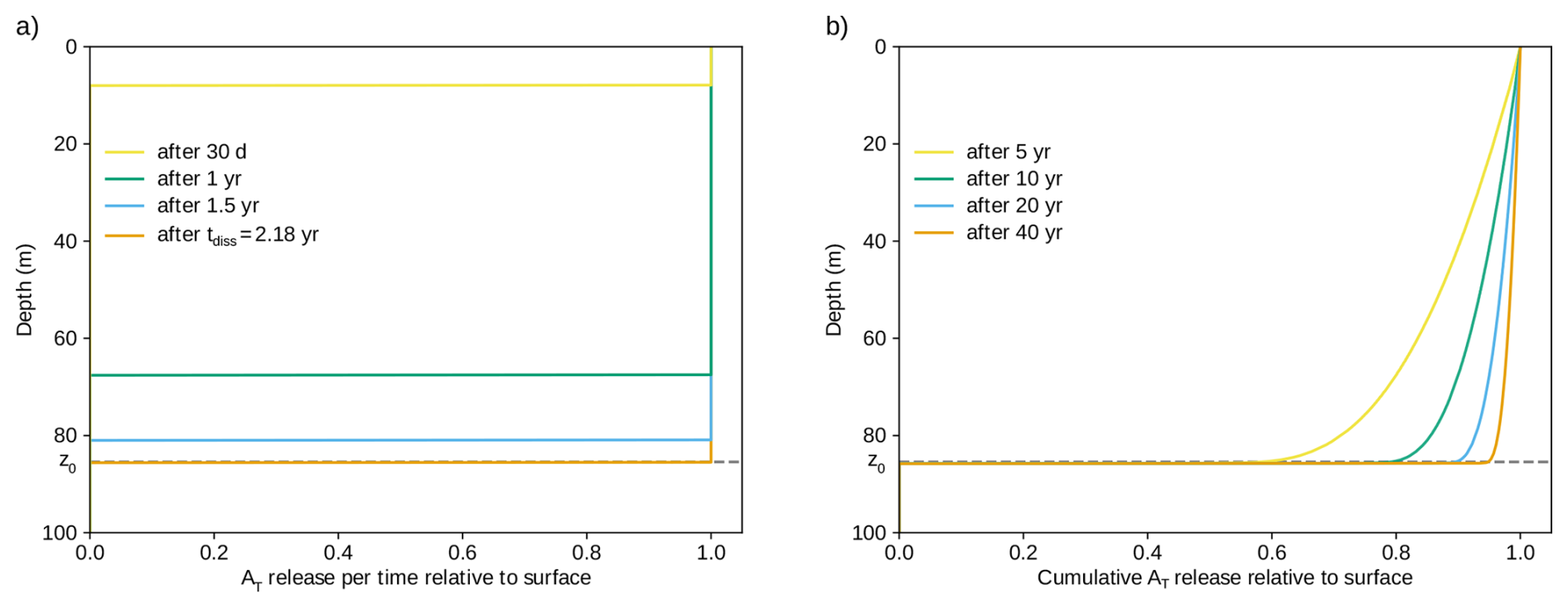
Figure A2 Numerical simulation used to validate the analytical uniform particle flux profile. Particles of diameter d = 1.7 µm are continuously added at the surface (T = 25 °C, pH = 8.2) and sink through a vertical grid of 0.1 m resolution with a timestep of 1 h. (a) The alkalinity release in each time step at different time points. The release is constant down to the depth the first-added particle reaches. At the dissolution time t_diss and afterwards, the alkalinity release profile extends down to the penetration depth z₀. (b) The cumulative alkalinity release is not strictly rectangular, since particles that were released less than t_diss = 2.18 years before have not reached z₀ yet and have only released alkalinity at shallower depths. For longer time periods since the start of the experiment, these particles matter relatively less, such that the cumulative alkalinity release is eventually also approximately rectangular. For example, the cumulative alkalinity released at depth z₀ is 95 % of that at the surface after 40 years.

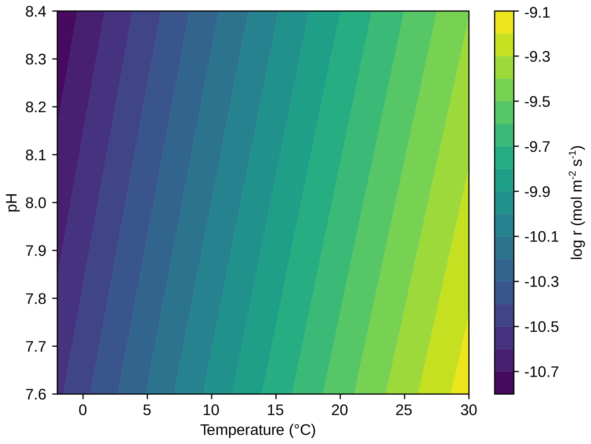
Figure A3 The base-10 logarithm of the area-normalized dissolution rate of forsterite determined for geometric surfaces from Rimstidt et al. (2012) as a function of temperature and pH.

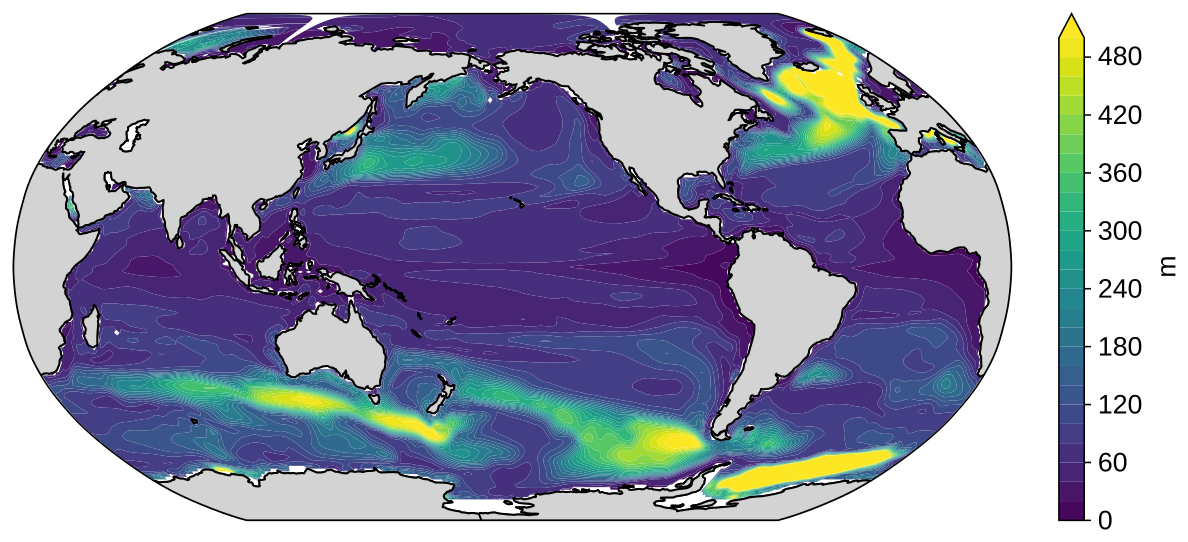
Figure A4 Annual maximum mixed layer depth in the GFDL ESM2M model. Mixed layer depth is defined as the depth where density increases by 0.03 kg m⁻³ relative to the surface. It is calculated as the annual maximum of monthly mixed layer depth, averaged over the period 2016-2025 and over five ensemble members. Global average annual maximum mixed layer depth is 123 m.

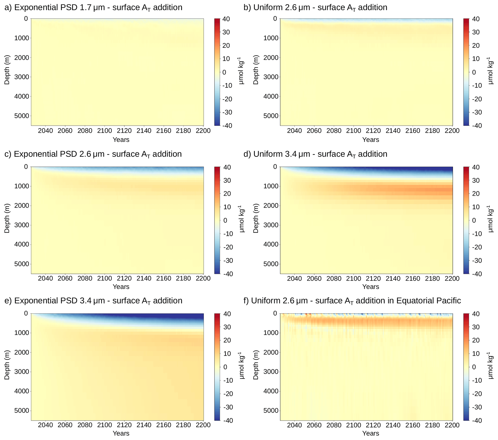
Figure A5 Global mean vertical distribution of additional alkalinity relative to that for surface alkalinity addition over time for the uniform and exponential PSDs with mean volume diameters of 1.7, 2.6, and 3.4 µm (panels a–e). We do not show the alkalinity difference for the uniform particle profile with d = 1.7 µm, as differences are minor. Panel (f) shows the alkalinity difference in the eastern and central equatorial Pacific (−8 to 8° N, −190 to −85° E) for the uniform case with d = 2.6 µm.

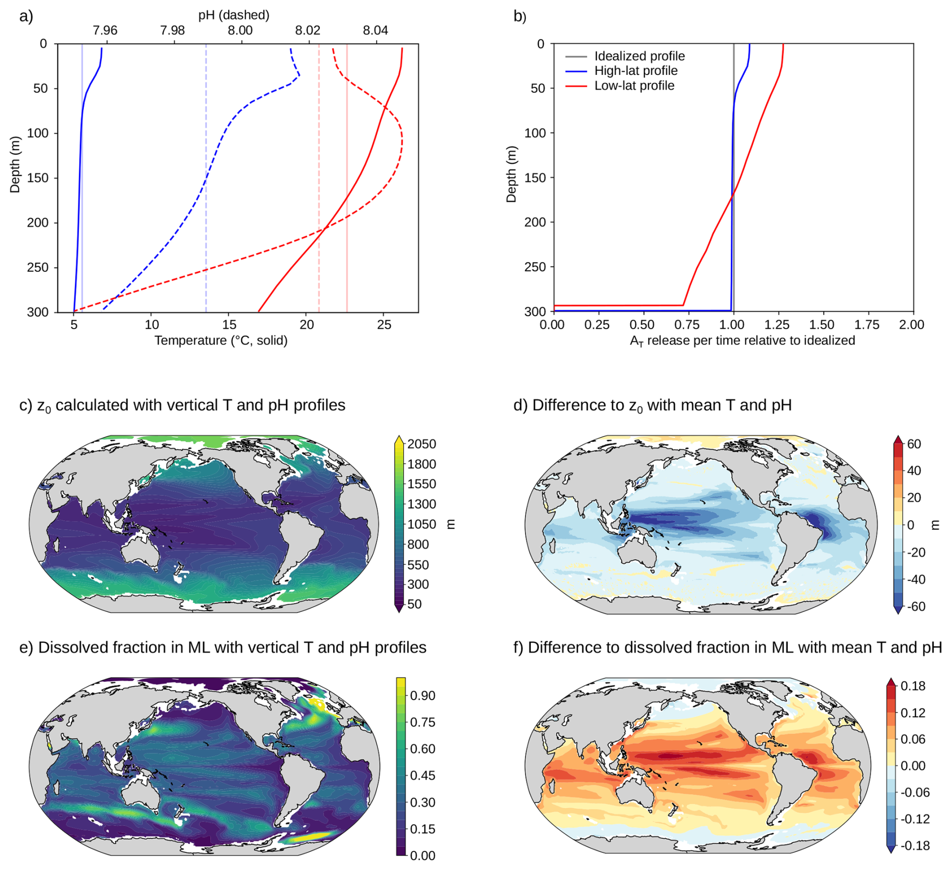
Figure A6 Numerical simulation used to test the influence of variations in temperature and pH (on the total scale) along the water column on the alkalinity release profile. Panel (a) shows two exemplary temporal mean profiles, one from the Southern Ocean (−57.5° N, 177.5° E) in blue and one from the subtropical Atlantic (20.9° N, −58.5° E) in red. Light vertical lines in panel (a) show mean temperature and pH over the upper 300 m. Under the idealized dissolution profile approach (Sect. 2.3), particles with a diameter of 1.7 µm in the subtropical Atlantic column and particles with a diameter of 2.6 µm in the Southern Ocean column both penetrate down to 300 m (penetration depth z₀ of 300 m). The numerical alkalinity release profiles with explicit vertical temperature and pH profiles are shown in panel (b). Panel (c) shows the penetration depth with explicit temperature and pH profiles for particles with diameter d = 2.6 µm globally, and panel (d) shows the difference to the penetration depth assuming mean temperature and pH (Fig. 2b). Regions where the water column is shallower than the penetration depth are left blank as they do not allow a direct comparison. Panel (e) shows the fraction dissolved in the annual maximum mixed layer with explicit temperature and pH profiles and panel (f) shows the difference to the dissolved fraction assuming mean temperature and pH (Fig. 2e).

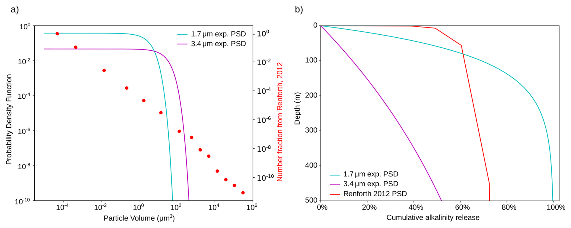
Figure A7 (a) Discretized sieve-based particle size distribution from Renforth (2012) compared to the exponential particle size distributions from this study for mean volume diameters of 1.7 and 3.4 µm, respectively. The PSDs are plotted on a log-log scale as that from Renforth (2012) spans many orders of magnitudes in particle volume, with its near-linear evolution resembling a heavy-tailed power-law distribution. (b) Cumulative alkalinity release over the upper 500 m assuming T = 25 °C and pH = 8.2.

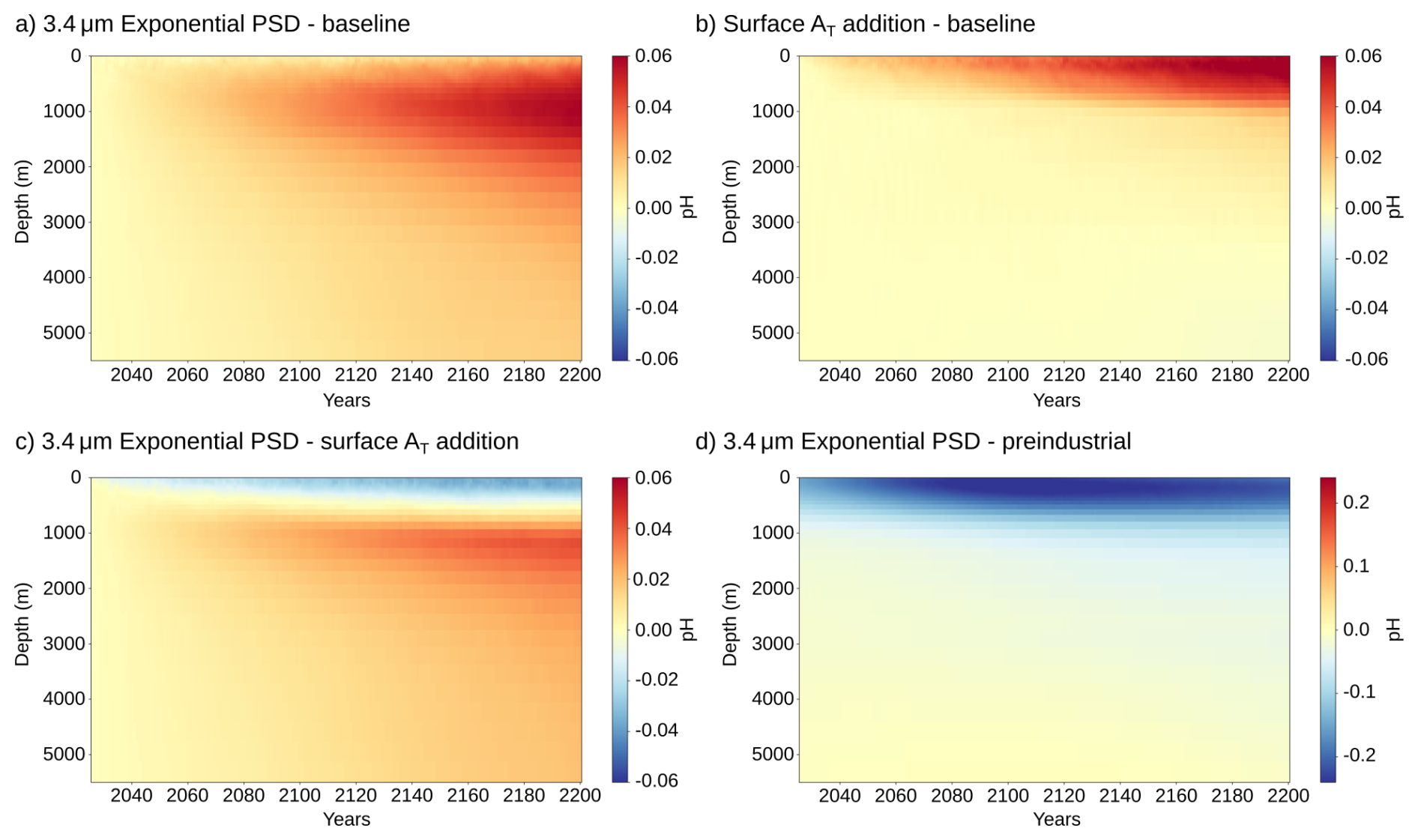
Figure A8 Global-mean pH difference along the water column between OAE and the baseline simulation without OAE, for (a) the exponential PSD with mean volume diameter of 3.4 µm and (b) surface alkalinity addition. The pH change is on the total scale and averaged over the period 2026–2200. Panel (c) shows the pH difference between the exponential PSD with mean volume diameter of 3.4 µm and surface alkalinity addition. Panel (d) shows the total change in pH from the baseline CO₂ emissions and OAE with the exponential PSD relative to the pre-industrial state.