The effects of peat thickness and water table depth on CO₂ and N₂O emissions from agricultural peatlands – a process-based modelling approach

Peatlands are critical carbon (C) reservoirs, storing over a fifth of the global soil organic C stock. However, some peatlands are drained and cultivated for agricultural use, which makes them a significant source of greenhouse gas (GHG) emissions. Managing water table depth (WTD) is considered a key operation for mitigating GHG emissions in cultivated peatlands. Modelling the impacts of water management would be a cost-efficient way of studying its large-scale effects, both in the present and in the future. Here, we used the process-based model LandscapeDNDC (LDNDC) to assess the relationships between WTD, peat layer thickness and the GHG exchange. We simulated a boreal agricultural peatland (NorPeat, Finland), which was cultivated with silage grass and barley during the study years 2019–2022. The site was monitored with an eddy covariance (EC) tower, and divided into six drainage blocks with distinct peat profiles, each equipped with sensors for continuous water table measurements. The model performance was evaluated on a daily and seasonal level using EC measurements of carbon dioxide (CO₂), nitrous oxide (N₂O) and water fluxes for the study years, alongside with satellite retrievals of the leaf area index and three-year data from block-specific dark chamber flux measurements of CO₂ and N₂O. The LDNDC model was found to be suitable for drained peatland simulations, although the performance was the highest when verified against measurements from shallow peat soils. Although the simulated N₂O fluxes were generally comparable with observations, their accuracy was not as high as it was for CO₂. To study the impact of WTD on GHG fluxes, we had three different scenarios in addition to the baseline runs with measured conditions; these scenarios had an average WTD of 50, 30 and 15 cm below the soil surface. The study results showed a clear relationship between CO₂ emissions and WTD (r=0.86 between exposed organic matter and net ecosystem carbon balance). GHG mitigation was achieved in all scenarios with increased water table; even in the most modest scenario, the annual reduction from the baseline was 5.8 t CO_2 e. ha⁻¹ in deep peat blocks and 2.5 t CO_2 e. ha⁻¹ in shallow peat blocks. CO₂ emissions were found to be more strongly affected than N₂O emissions. In the highest water table scenario, which resembled conditions close to paludiculture, the net ecosystem exchange of CO₂ was close to zero in most of the years, when fields were cultivated with forage grasses. The implications of raising the WTD were found to be insensitive to model parameters that control evapotranspiration or organic matter decomposition. These findings highlight that even moderate water management practices are valuable in order to mitigate GHG emissions in cultivated peatlands.

1 Introduction

Although peatlands cover only 3 % of the global land surface, they have a high carbon (C) density and are therefore considered critical C reservoirs, storing 21 % of the global soil organic C stock (Leifeld and Menichetti, 2018; Mander et al., 2024). In Europe¹, the peatlands are mainly found in the north, with Finland accounting for almost a third of peatland resources (Montanarella et al., 2006).

Peatlands are cultivated for their high organic matter (OM) content and ability to retain soil moisture even in drought periods. While many drained peatlands are favorable to agricultural use, cultivated peatlands are known to be a significant source of greenhouse gas (GHG) emissions (Tiemeyer et al., 2016). Pristine peatlands are naturally waterlogged, so when the peatland is drained for agriculture, it is no longer a notable source of methane (CH₄) or a sink of carbon dioxide (CO₂). Instead, as more organic matter is exposed to oxygen, CO₂ emissions increase through the microbial decomposition of peat, also known as heterotrophic respiration (Rh), and oxidation of CH₄ (Evans et al., 2021). In case of nutrient-rich peat, nitrous oxide (N₂O) emissions can also increase after drainage through nitrification and denitrification processes (Martikainen et al., 1993). However, CO₂ remains the largest contributor to the climatic impact of GHGs in drained peatlands (Dinsmore et al., 2009; Freeman et al., 2022; Gerin et al., 2023).

Raising the water table (WT) has been proposed as an effective strategy for mitigating GHG emissions from drained peatlands (Tiemeyer et al., 2016). Lång et al. (2024) estimated in their study in Finland that increasing the WT by 0.1 m reduced the soil respiration by approximately 0.1 kg CO₂-C m⁻² yr⁻¹ over an agricultural peatland. Similarly, Evans et al. (2021) found a strong correlation between effective water table depth (WTD), i.e. the average depth of the aerated peat layer, and net ecosystem productivity (NEP), which was calculated as the sum of the net ecosystem exchange of CO₂ (NEE) and the C removed by harvesting. Even though a clear relationship has been demonstrated between WTD and CO₂ emissions, the potential to reduce N₂O emissions by raising the WT has been more difficult to assess (Wilson et al., 2016a; Couwenberg et al., 2011). N₂O emissions are driven by many different abiotic and biotic processes, and these dynamics are shown to be influenced by diverse agricultural practices and meteorological events such as tilling and fertilization (Wang et al., 2021; Kandel et al., 2020; Leppelt et al., 2014; Cowan et al., 2025), and freeze-thaw cycles (Teepe et al., 2004; Maljanen et al., 2010; Wagner-Riddle et al., 2017). In addition, the nature of N₂O emissions is intermittent, i.e. short periods of high releases can contribute substantially to annual N₂O emissions (Flessa et al., 1998; Berglund and Berglund, 2011), which adds complexity in estimating and predicting N₂O emissions.

Although field observations of GHG fluxes have increased in recent decades, the frequency of chamber measurements (often conducted weekly, bi-weekly if not monthly) may lead to missed seasonal dynamics and introduce high uncertainties in annual estimates (He and Roulet, 2023; Barton et al., 2015). Continuous measurements using the eddy covariance (EC) technique can address this frequency issue, but are more challenging to implement due to their complexity and high equipment costs. On the other hand, modelling the soil processes and ecosystem responds to environmental changes is also challenging, particularly when employing empirical approaches that rely on observations and have a limited capacity to extrapolate beyond the observed range of conditions (Duarte et al., 2003).

Cost-efficient scaling up in space and time, as well as studying the effects of alternative management actions, requires models that take into account site-specific conditions, such as peat properties, management and climate. For this purpose, we can use process-based models, which are designed to replicate the key biochemical processes occurring in the ecosystem (Cuddington et al., 2013). These models provide a mechanistic framework for understanding how various biological, physical and chemical processes (e.g., photosynthesis, decomposition, and nutrient uptake) interact and contribute to biogeochemical dynamics which drive the exchange of GHGs. Process-based models specifically adapted for organic soils (e.g. Huang et al., 2021a; Premrov et al., 2021) have been successful at simulating GHG fluxes over agricultural peatlands. However, many general land ecosystem models remain untested for simulating agricultural peatlands, even if they include the necessary process descriptions. One such ecosystem model is LandscapeDNDC (the Landscape Denitrification-Decomposition model, later LDNDC), which has been shown to accurately simulate the GHG exchange (Haas et al., 2013; Liebermann et al., 2019; Sifounakis et al., 2024) over mineral soils. The model may provide a suitable basis for peat soil simulations, but its applicability has not yet been studied in northern agricultural peatlands.

The aim of this study was to assess the relationships between water table depth, peat layer thickness and GHG exchange. In addition, we wanted to determine how these relationships affect the potential of water table management to mitigate GHG emissions in northern agricultural peatlands. To address this, we had three specific research questions:

1. Is the LDNDC able to simulate daily CO₂ and N₂O exchange in northern agricultural peatland?

2. How does a raised WT impact the carbon balance and N₂O emissions, and does the mitigation potential depend on peat depth?

3. How sensitive is the simulated WTD effect on CO₂ emissions to changes in parameters that determine the organic matter decomposition and soil moisture dynamics?

To tackle these questions, we simulated an intensively measured and managed peatland site that has been monitored for GHG fluxes and hydrological and soil chemical properties since 2019. We calibrated the model to reproduce the seasonal and interannual patterns in the observed GHG exchange. The study site was divided into blocks with different peat depths, which furthermore enabled us to test the simulated relationships between peat depth and GHGs. Finally, we simulated counterfactual water table depth scenarios to evaluate the potential of water management to mitigate GHG emissions on the study site.

2 Materials and methods

2.1 Site

The study site is part of the Ruukki research infrastructure located in the North Ostrobothnia (Pohjois-Pohjanmaa) region of Finland (64°41.039^′ N 25°6.379^′ E) and managed by the Natural Resources Institute Finland (Luke). The NorPeat facility is a ca. 27 ha study field that is a former minerotrophic peatland drained in 1910s and cultivated since ca. 1920. The field has been continuously drained since the original drainage and drainage systems have been renewed multiple times from open ditches to subsurface drainage with wooden pipes, tile drains and modern plastic pipes. The most recent drainage works were made in 2014, when the drainage systems for each block were updated with adjustable weir to control drainage depth. Additional information on current drainage and geology of the site can be found in Yli-Halla et al. (2022).

The field is divided into eight drainage blocks, separated by a small sandy road in the center (Fig. 1). The focus is on blocks 1–6 as the detailed soil analysis was conducted only for these blocks. Blocks 1, 2 and 4 have a thicker peat layer ranging from 32 to 76 cm (on average 56 cm) while blocks 3, 5 and 6 have a thinner peat layer ranging from 16 to 56 cm (on average 34 cm). Blocks 5up and 6up have also a thinner peat layer similar to blocks 3, 5 and 6. The detailed soil properties of blocks 1–6 can be found in Table 1.

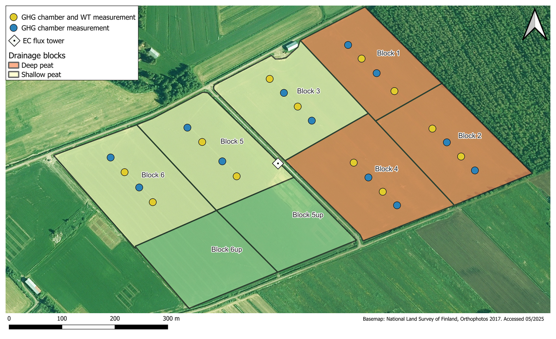
Figure 1 Study site with the different blocks highlighted by peat depth. Chamber measurements were done on blocks 1–6. EC measurements presented in this study include blocks 5, 6, 5up and 6up.

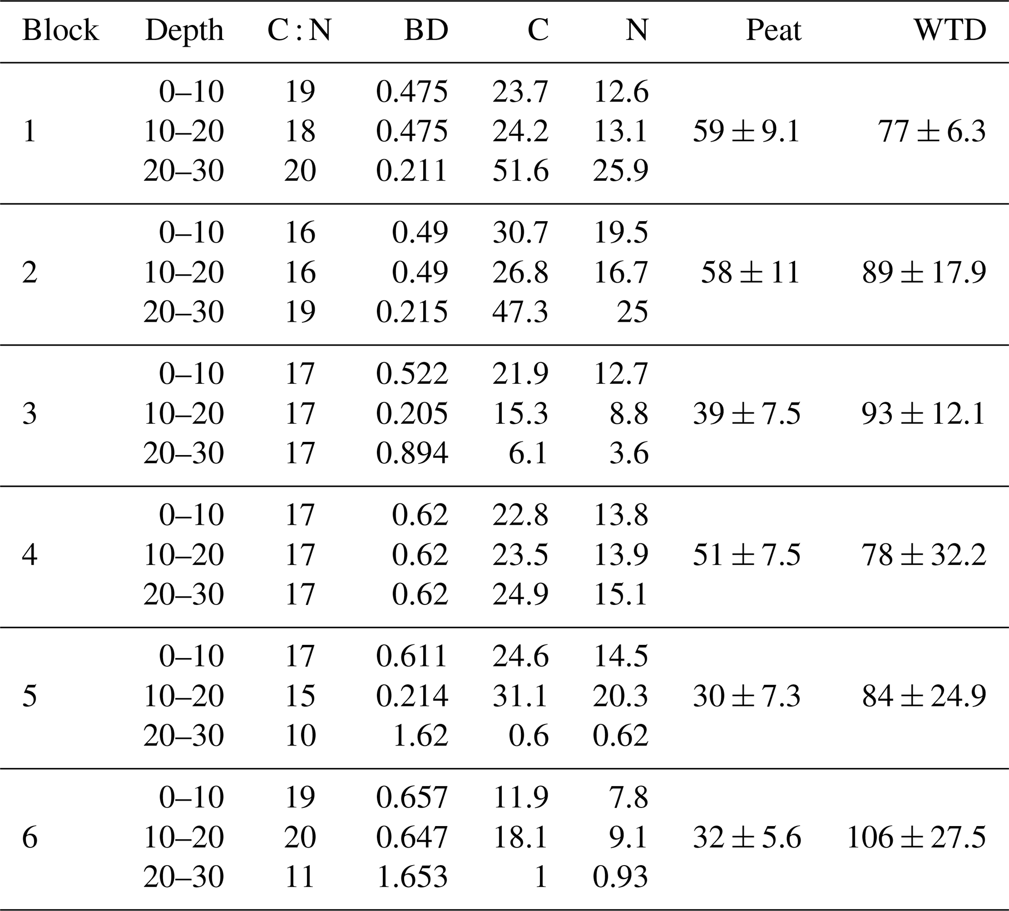
Table 1 Soil properties for each field block. C : N ratio, bulk density (BD, kg dw dm⁻³), carbon (C, %), nitrogen (N, g kg⁻¹) content from three sampling depths (Depth, cm) and mean peat thickness with standard deviation (Peat, cm). Original data from Yli-Halla et al. (2022) were recalculated by combining horizons. Samples were taken in 2020 from one replicate per block. WTD column shows average annual water table depth with standard deviation during 4 monitoring years used in the simulations.

The site follows a traditional grass-intensive crop rotation in which grass is cultivated for three to four years, followed by one or two years of cereal crops. The sown seed mixture contained timothy (Phleum pratense) and meadow fescue (Festuca pratensis). Until fall 2021, blocks 1–4 and 5–6 were at different stages of the crop rotation. Blocks 5–6 grew perennial grasses from 2018 to 2021 (first sown in 2017 with triticale as a nurse crop). In blocks 1–4, barley (Hordeum vulgare) was first cultivated in summer 2019, then the grass mixture was grown from 2020 to 2021. Blocks 5up–6up had the same crop rotation as blocks 5–6. In September 2021, glyphosate was applied to kill the vegetation in all blocks. In June 2022, the field was first ploughed and harrowed, followed by barley sowing a few days later. In September 2022, glyphosate was applied, and in October 2022, the field was ploughed. Every year, the field was fertilized and harvested once or twice. During barley years, the field was also sprayed with herbicides (Tables S8 and S9 in the Supplement).

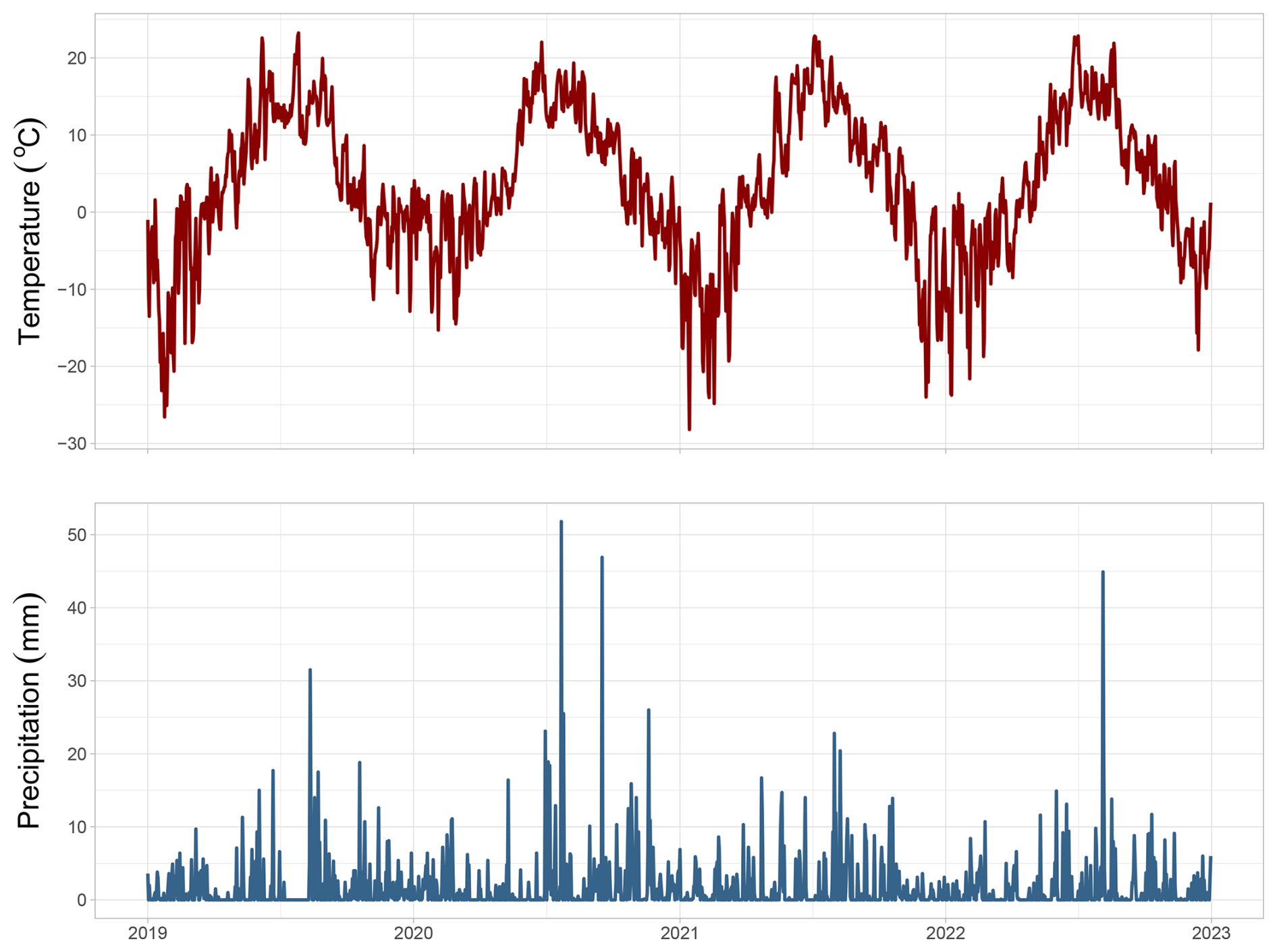
Figure 2 Average daily air temperature obtained from the study site and total daily precipitation obtained from the FMI weather station Siikajoki Ruukki (located within 1 km of our site) during the years 2019–2022.

Based on the FMI weather station Siikajoki Ruukki, located within 1 km of our site (Finnish Meteorological Institute, 2023), the long-term 1991–2020 mean annual temperature and total precipitation were 3.2 °C and 555 mm, respectively. From 2019 to 2022, the mean annual temperatures were 3.2, 4.7, 2.4 and 3.4 °C, while the total precipitation was 519, 732, 580 and 514 mm, respectively (Fig. 2, Table S7).

2.2 Measurements

2.2.1 Eddy covariance measurements, filtering and gap-filling

The eddy covariance tower was installed in the middle of the field (Fig. 1) on 13 June 2019. The measurements started at a height of 2.3 m, but it was raised to 3.15 m on 25 June 2019 and to 3.3 m on 4 November 2019, where it remained until the end of the measurement period (December 2022). Since the tower installation on 13 June 2019, the EC tower was equipped with a sonic anemometer (uSonic-3 Scientific, METEK Meteorologische Messtechnik GmbH, Germany) to measure wind speed in three dimensions and an enclosed-path non-dispersive infrared analyzer (LI-7200, LI-COR Biosciences, NE, USA) to measure CO₂ $/$ H₂O mixing ratios. On 4 November 2019, a continuous-wave quantum cascade laser absorption spectrometer (LGR-CW-QCL N₂O $/$ CO-23d, Los Gatos Research Inc., CA, USA) was installed to measure N₂O mixing ratio. The sampling frequency was 10 Hz, and the fluxes were averaged over a period of 30 min. Standard, well-established methods were used to calculate the 30 min turbulent fluxes. The details of the calculation and filtering procedures for CO₂ fluxes are described in Vira et al. (2025). The details of N₂O flux data processing are described in Gerin et al. (2023), except for the variance of N₂O mixing ratio, which was set to $\mathrm{5.5}\times {\mathrm{10}}^{-\mathrm{5}}$ ppm² for 2022. Due to the location of the instrument cabin and the dominant wind direction being from the southwest, 72 % of the filtered flux data came from blocks 5–6 from June 2019 to December 2022. Since there were also different crop rotations between blocks 1–4 and 5–6 (except for summer 2022), we decided to exclude the EC fluxes from blocks 1–4 in this study by discarding the flux data originating from wind directions 0–135 and 300–360°. In addition to wind direction filtering, we used a footprint model developed by Kljun et al. (2015) to estimate the cross-wind-integrated flux footprint distribution from the EC tower to the edge of the field, ensuring that the measured flux originated from the target area. The data were discarded if the cumulative footprint was less than 70 %.

N₂O fluxes were available from November 2019. First, gaps of two hours or less were gap-filled with linear interpolation. Days with at least four observations were averaged to daily integrals, while other days were discarded. Lastly, N₂O daily integrals were gap-filled using a moving average with a window size of 3 d which was increased as needed to include a least 2 adjacent observations (Gerin et al., 2023).

Half-hourly evapotranspiration (ET) was calculated and processed with the Eddypro software (v. 7.0.9, LI-COR Biosciences, USA) by applying similar filtering steps as described in Vira et al. (2025) for CO₂ but using steady-state flags and spectral corrections specific to the water flux.

2.2.2 Chamber flux measurements

Total ecosystem respiration (TER) and N₂O fluxes were measured weekly during snow-free seasons from 2019 to 2021 using the closed static chamber method. Metal collars (60 cm × 60 cm) with water grooves were permanently installed in the soil at the depth of 20 cm near the WTD measuring points. There were four replicates in each block. During the 45 min closure time, an opaque metal chamber with an air mixing fan was placed on top of the collar and four 20 mL gas samples were taken at 0, 15, 30, and 45 min and analyzed with a gas chromatograph (HP 7890 series, GC system, Agilent, USA) equipped with flame ionization (FID), electron capture detectors (ECD) and a nickel catalyst. Fluxes were calculated using linear regression.

2.2.3 Environmental variable measurements

Air temperature at the height of 1.6 m (Humicap HMP155, Vaisala Oyj) and soil moisture at the depth of −10 cm (ML3 ThetaProbe sensor, Delta-T Devices Ltd., Cambridge, UK) were continuously measured near the EC tower in block 5. Soil measurements during the winter time were unreliable and we therefore focus the model evaluation on conditions with non-frozen soils. In addition, soil moisture at −6 cm depth was measured concurrently with the chamber measurements in blocks 1–6 using an HH2 equipped with a ThetaProbe ML2x (Delta-T Devices Ltd., Cambridge, UK). WTD was monitored in blocks 1–6 using two perforated groundwater pipes installed in each block (Fig. 1) and equipped with Solinst Levelogger sensors (Solinst, Ontario, Canada), recording values at 15 min intervals (Pham et al., 2026).

The in-situ measurements were supported by remote sensing imagery from the European Space Agency's (ESA) Sentinel-2 satellite, which was used to estimate leaf area index (LAI). The LAI time series was processed and calculated using the methods described in Nevalainen et al. (2022) and European Space Agency (2016), using Level 2A reflectance data, the ESA Sentinel Application Platform (SNAP) Biophysical Processor neural network algorithm, and Google Earth Engine.

The performance of Sentinel-2 LAI retrievals has been tested extensively in recent studies (e.g. Brown et al. (2021); Kganyago et al. (2020)) and field observations from a southern Finnish site also showed good agreement with Sentinel-2-derived LAI estimates (Heimsch et al., 2024) supporting their general reliability. As the retrieval accuracy can vary spatially, we acknowledge that some uncertainty remains regarding the absolute LAI levels at our study site. However, we expect that the temporal dynamics of vegetation growth can still be assessed reliably.

2.3 LandscapeDNDC

We employed a process-based ecosystem model known as LandscapeDNDC to conduct the simulations in this study. The LDNDC is a well-established biogeochemical model derived from the DNDC model (Gilhespy et al., 2014). The LDNDC consists of several modules, each responsible for different ecosystem processes. Due to its high modularity, the model can simulate arable, grassland and forest ecosystems, the first one being the focus of this study. The model includes a layer-wise representation of biogeochemical (carbon and nitrogen cycling) and physical (moisture and heat) processes within the soil profile. This makes it well-suited for studying how these processes respond to variations in drivers such as water table depth and how the responses are affected by soil stratification.

2.3.1 Model overview

In this study, we focused on the interactions between GHG fluxes, the water cycle and the growth of vegetation. We used the PlaMo^x plant growth module (Liebermann et al., 2019), which simulates the carbon and nitrogen cycles in vegetation as affected by soil characteristics (nitrogen uptake) and the water cycle (transpiration). The meteorological data (e.g. temperature, radiation), which PlaMo^x uses to calculate carbon uptake, were processed for the canopy layers using the CanopyECM module (Empirical Canopy Model;  Grote et al., 2009). CanopyECM also simulates the soil temperature (Kraus et al., 2015). Each plant type is characterized by a distinct parameterization that governs its responses to key environmental drivers such as radiation, soil moisture and temperature. We cover the parametrization in Sect. 2.3.2 for the parts that deviated from the default settings.

In addition, we used the MeTr^x module (Metabolism and Transport of x;  Kraus et al., 2015; Petersen et al., 2021) to simulate carbon and nitrogen cycles in the soil. MeTr^x describes the turnover of litter and soil organic matter using six carbon and nitrogen pools. These are discretized according to the input discreatization of the soil profile along with the pools of inorganic nitrogen (ammonium and nitrate) and dissolved organic carbon and nitrogen. The model simulates the biogeochemical effects of waterlogging by evaluating the C and N cycling processes separately for the aerobic and anaerobic volume fractions in each soil layer. The anaerobic volume fraction is diagnosed from the oxygen partial pressure, which in turn is solved explicitly from the layer-wise profiles of oxygen diffusivity and consumption. N₂O-forming processes (nitrification and denitrification) are simulated based on nitrifier and denitrifier growth and are dependent on substrate and oxygen availability, microbial activity and soil pH. The effect of tillage is simulated by homogenizing the C and N pools within the tillage depth and by temporarily accelerating the organic matter decomposition as described in Haas et al. (2022).

Finally, the soil moisture was simulated using the WatercycleDNDC module (Kiese et al., 2011; Petersen et al., 2021) in combination with a prescribed WTD as described in Sect. 2.4.4. The prescribed water table was assumed to capture the effect of tile drainage, which cannot be explicitly simulated by the LDNDC. The WatercycleDNDC handles the soil water movement above the water table, and accounts for the amount of precipitation intercepted by foliage, infiltration, percolation, transpiration, runoff, and possible changes in snow cover and ice content in the soil. The soil water movement is simulated using layer-specific field capacity and wilting point, which are derived from a soil water retention curve defined by the van Genuchten parameterization, and saturated hydraulic conductivity. The upper boundary condition for soil moisture is atmospheric, driven by infiltration and evapotranspiration, and the lower boundary is a free drainage condition. Precipitation is assumed to be snow when temperature drops below 0 °C, and the evolution of the snow cover and ice content are simulated based on meteorological conditions such as air temperature and precipitation. Actual evapotranspiration is limited by water availability and is therefore calculated as the minimum of potential evapotranspiration and the available water at the surface or in the upper soil layer.

For this study, we applied version 1.36 of the model (revision 11770). One of the main updates in this version affected the initialization procedure for soil C and N pools, which are typically initialized such that the overall soil organic matter stocks are near equilibrium. The version 1.36 adds an option to relax the equilibrium assumption by the possibility to prescribe an annual target value of organic matter accumulation or loss during the spin-up years. This is relevant for drained peatlands, which are typically not in equilibrium due to the continuing decomposition of the accumulated peat. This was implemented by introducing a new parameter (spinupdeltac) to the MeTr^x submodel, which enables users to align long-term changes in simulated C pools with those derived from historical observations. The default value of spinupdeltac is 0, corresponding to the original equilibrium assumption, but it can now be set to reflect user-defined annual changes (see Sect. 2.4.1).

2.3.2 Parameters

We made adjustments to certain site and species parameters to improve the model performance in our simulated study site. Since all of the simulated blocks had the same changes, there were no differences in the parameterisation between the blocks.

The original humus pool structure was designed for mineral soils, where mineral association of organic carbon provides strong protection even under aerobic conditions. The low decomposition rates of the two older humus pools reflect the increasing recalcitrance of more strongly humified and mineral-associated organic carbon typical of mineral soils. In peat soils, however, once aerated, organic matter decomposes more rapidly and carbon losses are higher than would be expected for mineral soils. Although the general oxygen response of decomposition is already implemented in LDNDC, the intrinsic turnover properties of the humus pools, particularly the two older humus pools containing most of the carbon, were too conservative to represent peat adequately. Therefore, the decomposition constants (METRX_KR_DC_HUM) of these older recalcitrant humus pools were increased to better reflect the higher aerobic decomposability of peat. The initially lower decomposition rate constant was increased more than the higher rate constant, leading to more similar absolute rate constants than in the default parametrization. As a result, blocks with similar carbon stocks exhibited comparable respiration rates despite differences in how the initialization procedure allocated carbon among the pools. Other changes to the site parameters were an increase of the maximum potential evapotranspiration. This matched the estimated evapotranspiration levels at the site and improved the seasonal change in the moisture levels near soil surface. Finally, we adjusted a site parameter controlling the fraction of surface water removed by runoff over each time step. The value was selected based on the study (Yli-Halla et al., 2022), which suggested that 30 % of the total drainage would be due to the surface runoff on the study site.

Among the crop-specific parameters, we made changes to both forage grasses, which we refer as grass from now on, and barley. We simulated the mixture of timothy and fescue together as a generic perennial grass during the grass years. For the grass, we adjusted parameters handling the photosynthesis activity (H2OREF_A) and stomata closing (H2OREF_GS) at drought. H2OREF_A is the parameter that defines the soil water content at which drought begins to reduce photosynthetic activity. H2OREF_GS defines the relative available soil water content at which stomata are fully closed. With default parametrisation the gross primary production stopped in some blocks (including block 5 where EC-tower was located) in the driest periods, when the soil moisture in the top soil layers dropped close to the wilting point. The growth of above-ground biomass and leaf area was simultaneously suppressed. The observed data did not indicate any drought: neither EC-based gross primary production (GPP) nor satellite-derived LAI showed any signs of suppression. Therefore, the parameters H2OREF_A and H2OREF_GS were set close to zero (10⁻⁶) to avoid underestimating the GPP in simulations. Furthermore, the species-dependent albedo factor (ALB) and maximum water use efficiency (WUECMAX) were adjusted to improve the seasonal changes and annual outputs in GPP. In addition, we modified the senescence parameters to reduce overestimation of LAI and consequently photosynthesis in the simulations. Increasing senescence due to frost stress was essential for capturing the decrease in LAI at the onset of frost. Finally, the perennial grass plant type was also used to simulate weeds during pre-sow and post-harvest periods in year 2022. However, to prevent it from dominating GPP output, we set the SLAMAX parameter value for it to 2.

For barley, we had similar objectives for parameter changes as for grass. We modified the growing degree day (GDD) thresholds that determine when crops enter different growth stages. These adjustments were necessary to align crop phenology with local climate conditions. We also increased the decline of specific leaf area parameter (SLADECLINE) at the end of the crop life cycle to prevent overestimation of GPP during late growing season. In addition to modifying the SLAMAX and senescence parameters, we increased the harvest index in barley to simultaneously match the reported harvest levels and the GPP derived from the EC measurements.

All modified parameters are shown alongside the model's default values in the Table S1.

2.4 Model setup

We set up model simulations for the six blocks at the site for the years 2010–2022, with the years 2010–2016 set as spin-up years. Each block had four different scenarios: the base scenario representing the observed WTD and three other scenarios with manipulated WTDs, to evaluate the effect of the WTD on GHG fluxes. These scenarios are described in detail later in the Sect. 2.4.4. In addition, each block and its scenarios underwent runs with some site or species parameters modified to estimate the sensitivity of the model to these parameters. All runs shared the same climate data, as detailed in Sect. 2.4.3. Each block had its own soil profile and management events. The layer-wise representation of the soil profile covered a depth of two meters. The upper soil layers were parameterized to reflect the characteristics of peat, including carbon and nitrogen content, bulk density, pH, and hydrological properties. The bottom layers represented silty mineral soils. The simulated soil layers were between 2 and 30 cm thick, with the thinnest layers at the top. The layer-specific parameters are explained in Sect. 2.4.1. The initialisation and management setups remained unmodified for each scenario in order to study the effects of changes in WTD and the model parameters.

2.4.1 Site initialisation and soil properties

Soil initialisation covered hydrology and soil composition features. Hydrological aspects were controlled with van Genuchten parameters α and n (based on Mualem (1976)), porosity, hydraulic conductivity, and the minimum water-filled pore space in the soil layer. The van Genuchten parameters were used to reflect a typical water retention curve for peat. This process was performed iteratively by starting from literature values (Menberu et al., 2021) and evaluating the response in the simulated soil moisture. The van Genuchten α parameter ranged from 0.75 to 6.0: the lower values associated with the organic matter layers in order to reproduce the slow drainage and high water retention. The van Genuchten n parameter, which affects the steepness of soil moisture curves, was set between 1.2–1.5 depending on soil layer and block. Even though some of the selected van Genuchten parameters differed significantly from the values reported by Menberu et al. (2021) for peatlands drained for agriculture, the meta-analysis (Liu and Lennartz, 2019) examining the hydrology in peat soils emphasised the parameters' complex relation and stressed that bulk density and stage of decomposition can significantly affect parameter values. The meta-analysis also indicated a large variation in these parameters across the published studies. The porosity was set lower in the silt soil layers beneath the peat layers due to the fine-textured characteristic of silty soils. In the soil samples taken below the peat layers, the porosity was measured to be around 0.4, which we used as a point of reference for our estimates. Finally, the hydraulic conductivity was set to range from 0.00045 to 0.005 (cm min⁻¹), where the highest values apply to the peat layers as the pore size and peat structure support faster water flow than in silty subsoil. These values were based on unpublished datasets from the site and further adjusted to produce representative soil moisture dynamics.

Soil carbon and nitrogen contents for each model layer were initialised based on values measured in soil samples (down to 200 cm) conducted in spring 2020 by Yli-Halla et al. (2022) (see supplement). The values for pH (4.4–6.1) and bulk density (0.15–1.65) were also from the same dataset. The annual C change during the spin-up years (spinupdeltac) was set to −4.5 t C ha⁻¹ for all blocks, which was approximately the C loss estimated on the shallow peat blocks 5 and 6 from the observed NEE and harvest yield (Gerin et al., 2023) in years 2020–2021. However, the loss of C was also affected by the parametrisation changes, and therefore resulted in larger annual C depletion, especially in the deep peat blocks where the annual loss was up to 10 t C ha⁻¹ in individual study years. We extrapolated the C and N amounts independently for each block to account for carbon depletion during the spin-up years; thereby aligning the simulated C and N stocks with the measurements for the year 2020. The extrapolation was performed in the baseline setup (i.e. no water table changes or sensitivity analysis), and the resulting site setup was shared among all subsequent runs. The complete site initialisation for each block can be found in Table S5.

2.4.2 Management

All management activities for 2019–2022 were straightforward to incorporate into the model runs as the dates of the events and possible seed and fertilizer amounts were given. Tillage depth and cut height in the field were not specified, but we kept them consistent (20 and 10 cm, respectively) across blocks. Glyphosate was applied in autumn 2021 and 2022 to terminate the grass stand and the weeds; this was simulated as a harvest event where 99 % of biomass was left on the field as residue. The last 1 % of biomass was removed from the field. The application of herbicide in July 2022 was furthermore taken into account by limiting the LAI of weeds (see Sect. 2.3.2). Additionally, due to technical limitations in handling organic fertilizers, we included the organic manure applied to some fields in 2019 as a mineral fertilization event, considering only the nitrogen input to the field. During the spin-up years, all simulations were run with perennial grass which was mowed twice a year.

2.4.3 Meteorology

For the driver (climate) data in the simulations, we used air temperature measured near the EC tower and the other meteorological data from the FMI weather station Siikajoki Ruukki located within 1 km of our site (Finnish Meteorological Institute, 2023); the shortwave radiation data was extracted from the Copernicus European Regional Reanalysis (CERRA;  Ridal et al., 2024). For the spin-up years (2010–2016), we furthermore used three-hourly data extracted from ERA5 reanalysis (Hersbach et al., 2020). The data from different sources were converted to hourly data to match the time steps of the simulations. For ambient GHG concentrations, we used values of 415 ppm for CO₂, 2 ppm for CH₄ and 330 ppb for N₂O. The ambient concentrations for CH₄ and N₂O are required as boundary conditions for evaluating the diffusion and consumption of these gases in the soil. The concentrations are similar to those measured at different locations in Finland (Finnish Meteorological Institute, 2025). Other air chemistry-related inputs were kept as default in the model.

2.4.4 Water table depth

A prescribed WTD was used in all simulations. In this mode, the model forces a saturated soil water content for layers below the WTD and simulates the soil water flow above the water table. In the baseline simulations, the WTD was specified by a measured time series. Since WTD measurements were available from May 2018 onwards, we used the averaged hourly values from May 2018 to December 2022 to represent the missing data period (i.e., January 2010–May 2018) in the spin-up simulations. This was done to provide a realistic representation of WTD variations, while taking into account seasonal changes.

Water table scenarios were applied to the period for which we had the measured data. In the baseline scenario, no changes were made to the water table, while the three counterfactual water table scenarios used scaled WTDs, WTD_scale which preserved the seasonal and annual hydrological variation and responses to precipitation events. These were created by uniformly rescaling original water table observations WTD_obs. with the ratio of target average water level WTD_target. (15, 30, and 50 cm) and long term mean WTD WTD_mean below the soil surface:

$$\begin{array}{}\text{(1)}& {\mathrm{WTD}}_{\mathrm{scale}}={\displaystyle \frac{{\mathrm{WTD}}_{\mathrm{target}}}{{\mathrm{WTD}}_{\mathrm{mean}}}}\cdot {\mathrm{WTD}}_{\mathrm{obs}.}\end{array}$$

Examples of the measured water table and scenarios for Block 5 are shown in Fig. 3.

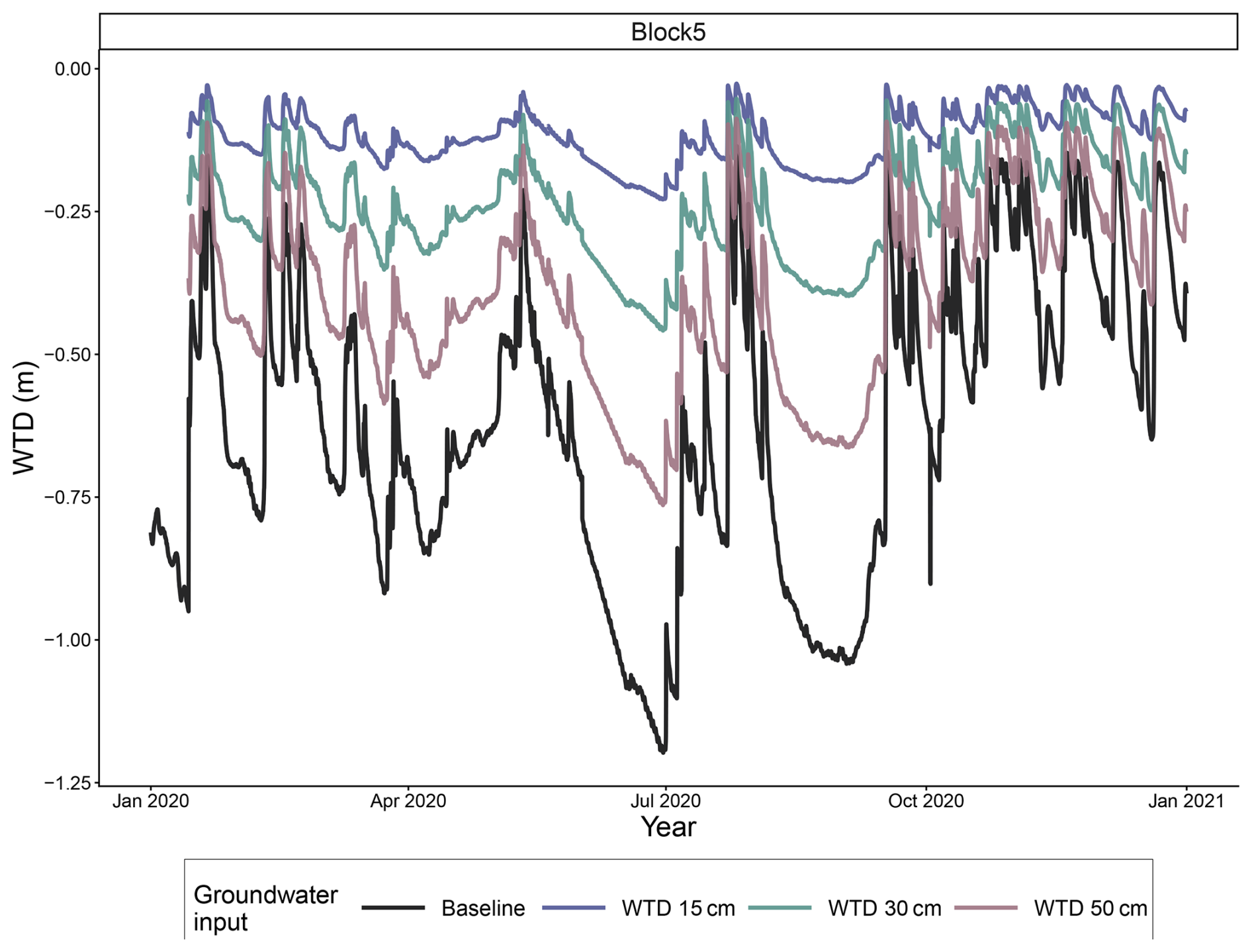
Figure 3 Water table depths (WTD) in year 2020 for the baseline and scenario simulations in block 5. May 2018 onward the WTDs for scenarios were on average 15, 30 and 50 cm below soil surface. All of the counterfactual water table scenarios (15, 30, and 50 cm) followed the dynamics of the measured WTD.

2.5 Model evaluation and performance metrics

We evaluated the model performance for simulating NEE, N₂O emission, and evapotranspiration by comparison against the EC measurements. Although the EC measurements covered the blocks 5, 5up, 6 and 6up, these measurements are addressed only against blocks 5 and 6 as blocks 5up and 6up are not considered in this study. We furthermore compared the predicted soil water content against the field measurements and evaluated the simulated leaf area index against the satellite retrievals both described Sect. 2.2.3. These comparisons were performed on up to daily time resolution as determined by availability of observations.

The evaluation against EC data was supplemented by comparing the simulated ecosystem respiration against the chamber measurements conducted across the blocks with differing peat thickness (Sect. 2.2.2). This comparison was based on simulated daily averages; we did not try to to reproduce the 45 min chamber closures with the model, in part because we lack mechanisms to accurately simulate short term responses of the plant respiration to temporary darkness (e.g. Tcherkez et al., 2017), and in part due to the more general uncertainties in simulating carbon allocation on a sub-daily level (Sierra et al., 2022). Although the respiration fluxes measured by the chambers are likely to differ from the daily mean, we consider this tradeoff acceptable given that the chamber measurements are here used mainly to quantify the spatial variation of the respired CO₂.

Finally, between the water table scenarios we compared the differences in heterotrophic respiration, as well as in autotrophic respiration and CO₂ uptake, to inspect the water table relation to these factors. In addition, we examined the modeled annual nitrification, which controls the availability of nitrate for denitrification, to understand response of N₂O to the WTD scenarious. We evaluated the model performance based on the metrics defined below.

2.5.1 Nash-Sutcliffe Efficiency

Nash-Sutcliffe Efficiency (NSE) is commonly used to evaluate the effectiviness of hydrological models (Krause et al., 2005). The equation for NSE is similar to the equation to calculate the coefficient of determination for regression models, where it is used to estimate the proportion of variance that the model is able to explain. The difference between R² on the regression model and NSE is the interpretation of the results. The NSE estimates the predictive power of a simulated model and focuses on the accuracy of the predictions compared to the observed values. Since the predictive values are simulated, the range of the results varies from −∞ to 1 (perfect fit), where a value of 0 indicates that the model does not succeed any better than taking the mean value of the observations. The equation for NSE is

$$\begin{array}{}\text{(2)}& E=\mathrm{1}-{\displaystyle \frac{\sum _{i=\mathrm{1}}^n(O_i-P_i{)}^{\mathrm{2}}}{\sum _{i=\mathrm{1}}^n(O_i-\stackrel{\mathrm{‾}}{O}{)}^{\mathrm{2}}}},\end{array}$$

where the O_i was observed value and P_i was simulated value. Variable $\stackrel{\mathrm{‾}}{O}$ was the mean of the observed values.

2.5.2 Linear regression and bootstrapping

We used the function lm() from R package stats (R Core Team, 2024) to quantify the linear relationship between obtained CO₂ values from chamber measurements and the simulated CO₂ values. We studied the differences in the relationships that shallow peat and deep peat had to measured values. The linear regression model was expressed as

$$\begin{array}{}\text{(3)}& \mathit{O}=k\mathit{S}+\mathit{ϵ},\end{array}$$

where the O was the vector of observed values and S was the vector of simulated values. In practice, as there were up to four chamber measurements simultaneously taken, the simulated vector S contained duplicate values for each observed value. Vector ϵ included error terms as the function seeks to minimize the sum of squared error terms by using the least square method to estimate the slope k. As seen in the Eq. (3), the intercept was set to 0 as we wanted to analyse the differences in the slope k. Confidence intervals (CI) for the slope difference were calculated using the R package boot (Angelo Canty and B. D. Ripley, 2024) with 3000 bootstrap samples.

2.6 Sensitivity analysis

An additional set of simulations was run to assess the robustness of the simulated differences between water table scenarios with respect to model parameters that influence soil biogeochemistry and water content. We perturbed three organic matter decomposition rates (METRX_KR_HUM 1, 2 and 3) and two parameters affecting evapotranspiration (potential evaporation fraction and WUECMAX) by individually decreasing or increasing the parameter value by 30 % of its value in the baseline simulations. These parameters are a subset of those adjusted in Sect. 2.3.2. Since the impact of these perturbations can be expected to interact with the impact of the water table scenarios (Sect. 2.4.4), we ran the perturbed simulations separately for each water table scenario. Finally, we evaluated the response of the treatment effect (scenario versus baseline) to each parameter perturbation to provide an estimate of how sensitive the simulated GHG mitigation was with respect to the model parametrization.

2.7 Net ecosystem carbon balance and CO₂ equivalents

We calculated the net ecosystem carbon balance (NECB) as

$$\begin{array}{}\text{(4)}& \mathrm{NECB}=\mathrm{NEE}+{\mathrm{C}}_{\mathrm{export}},\end{array}$$

where C_export denotes the carbon removed in harvest. Other components that affect the NECB include organic fertilization, leaching of dissolved carbon, and the atmospheric exchange of methane. We did not include these fluxes, because organic fertilizers were not simulated or used in the years covered by the EC measurements. In addition, the contributions of methane and leaching were found to be small compared to CO₂ based on earlier data on the same site (Yli-Halla et al., 2022).

Finally, to study the contribution of CO₂ and N₂O in the total climate impact of the peatland cultivation in each water table scenario, the N₂O balances (i.e. annual sum of N₂O fluxes) were converted to CO₂-equivalents (CO_2 e.) by applying the sustained global warming potential (SGWP) coefficient of 270 mol CO_2 e. per mol N₂O over a 100-year time horizon (Neubauer, 2021).

3 Results

3.1 Applicability of LDNDC

3.1.1 Water cycle and leaf area index

To assess the model performance, we first compared the simulated water cycle and LAI in the baseline runs (driven by the measured water table depth) to the observations. The model captured the seasonal changes in the water content in the top soil layers (Figs. 4, S2 in the Supplement). However, especially in block 1, a temporal shift was observed between the measurements (taken together with chamber flux measurements) and the simulations, as the measurements indicated that the soil was drier than simulated in the beginning of the summer. This was also reflected in the statistics for soil moisture, as the R² and NSE for block 1 were 0.43 and −0.24, respectively, while the same values for the rest of the blocks were 0.36–0.75 and from 0.06 to 0.75, respectively. The highest R² and NSE were obtained for blocks 5 and 6, where the EC tower flux data was also collected.

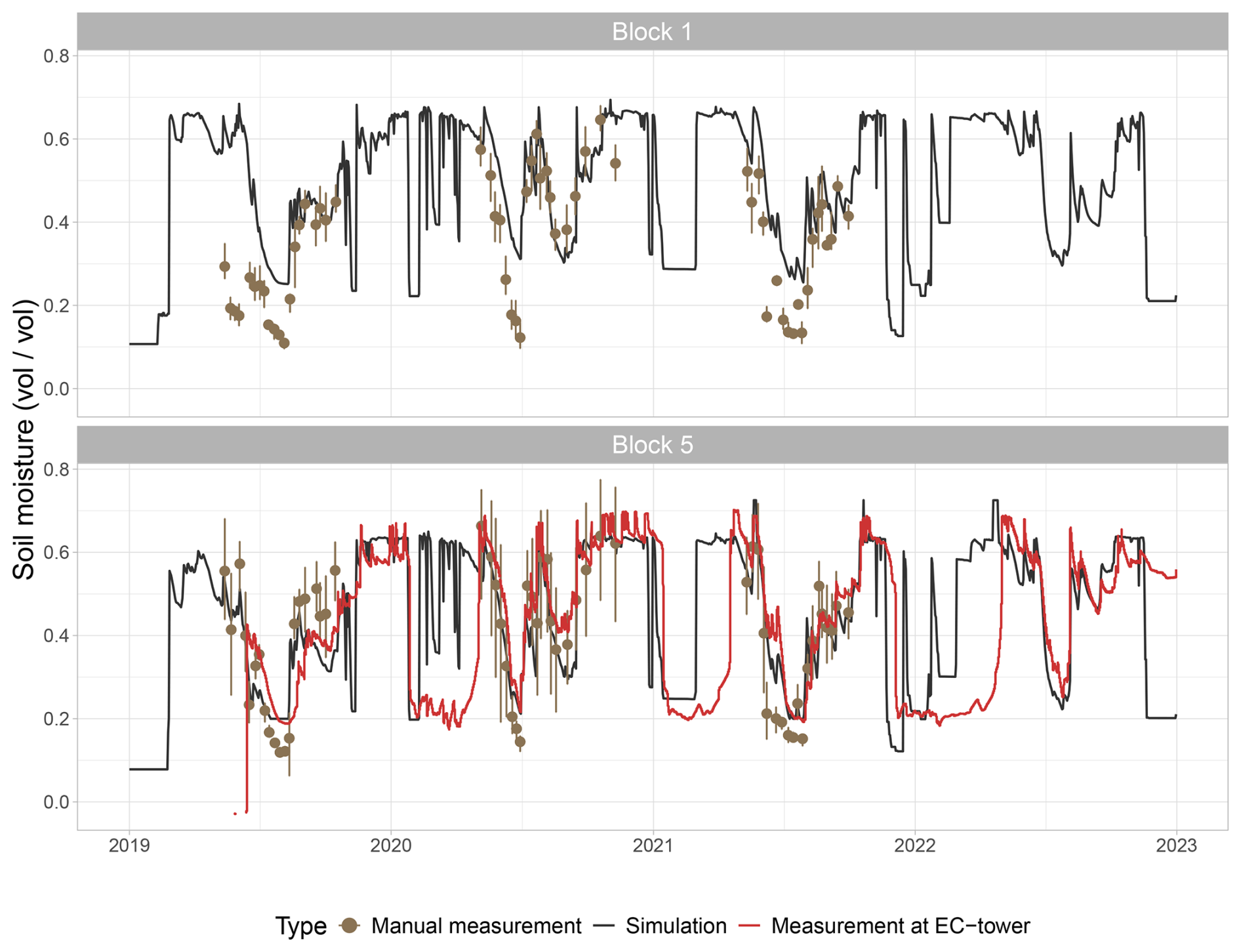
Figure 4 Measured and simulated volumetric soil moisture (m³ m⁻³) in blocks 1 and 5. Manual measurements at the flux chamber locations are shown with round markers; simulations and measurements at the EC tower are shown with lines. Each marker for manual measurements represents the average value of four measurements taken at a given time point at a depth of 5 cm, and the error bars indicate the minimum and maximum values of these measurements. The simulations and measurements at the EC tower represent the depth of 10 cm.

The evapotranspiration simulated for blocks 5 and 6 generally reproduced the seasonal variation of the EC measurements (Fig. 5; R² were 0.69 and 0.65, respectively, for these two blocks, and between 0.60–0.63 for the rest). The simulated yearly mean evapotranspiration from blocks 5 and 6 (1.37–1.41 mm d⁻¹) were slightly higher than the observations (1.11–1.20 mm d⁻¹) for the grass years, but for the cereal year 2022 the predicted average evapotranspiration was approximately 70 % higher than the observed (0.96 mm d⁻¹).

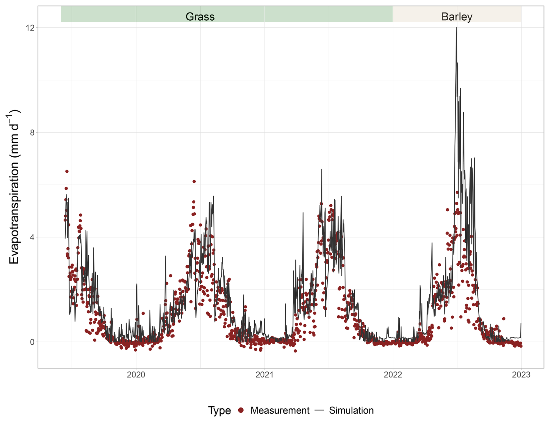
Figure 5 The EC measured (dots) and simulated (line) daily evapotranspiration (mm d⁻¹) for the years 2019–2022. The simulated values are averages from blocks 5 and 6. Colors indicate forage grass years (green) and cereal year (beige).

The temporal dynamics of the simulated LAI values agreed well with the observations (R² ranging from 0.57 to 0.66; Fig. 6), as the start of the growing season and increase of LAI after the cuts were captured in the simulation. The model also captured the leaf area decline at the end of the cereal years, when the crop started to reach harvest maturity. However, even though the model predicted yearly peaks of LAI well for the grass year, the peaks at cereal years were about 40 % of the peaks retrieved from the satellite data.

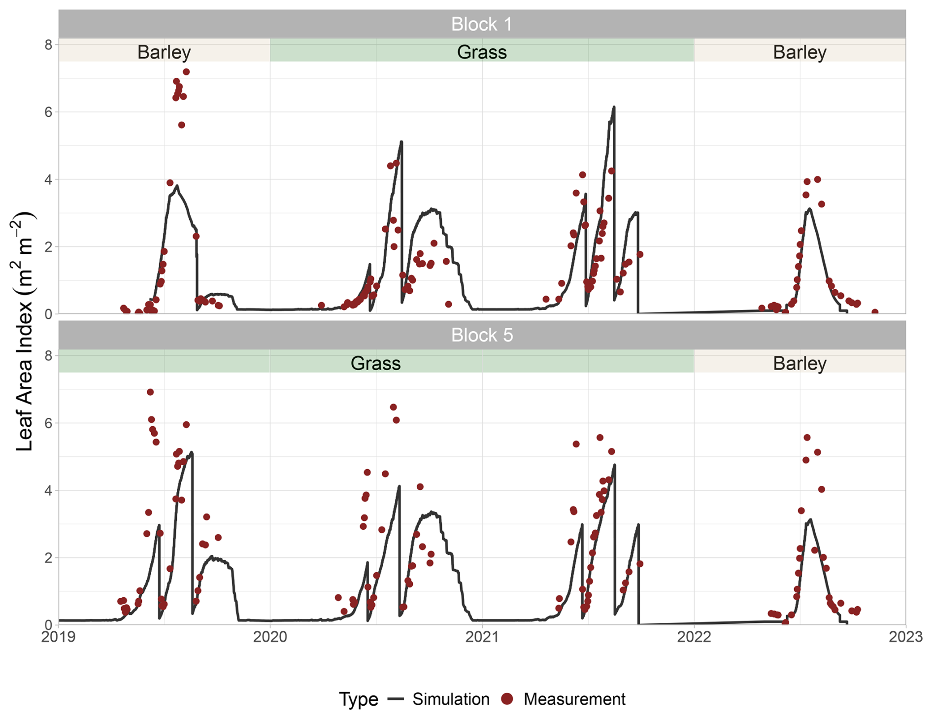
Figure 6 Satellite-retrieved (dots) and simulated (line) Leaf Area Index (m² m⁻²) for blocks 1 and 5 during 2019–2022. Colors indicate forage grass years (green) and cereal years (beige).

3.1.2 GHG fluxes and balances

The simulated TER generally agreed well with the chamber measurements (R²=0.56; Fig. 7). However, the modeled respiration fluxes were slightly underestimated for the shallow peat blocks and overestimated for the deep peat blocks. This can be seen in the regression slopes, which were above 1 (1.1–1.19; 95 % CI) for the shallow peat blocks (3, 5, 6) and slopes below 1 (0.87–0.93) for the deep peat blocks (1, 2, 4). These values differ slightly from the numbers shown in Fig. 7 as the regression lines were fitted over all of the data points from shallow and deep peat blocks. The 95 % CI for the difference between the slopes was 0.20–0.30.

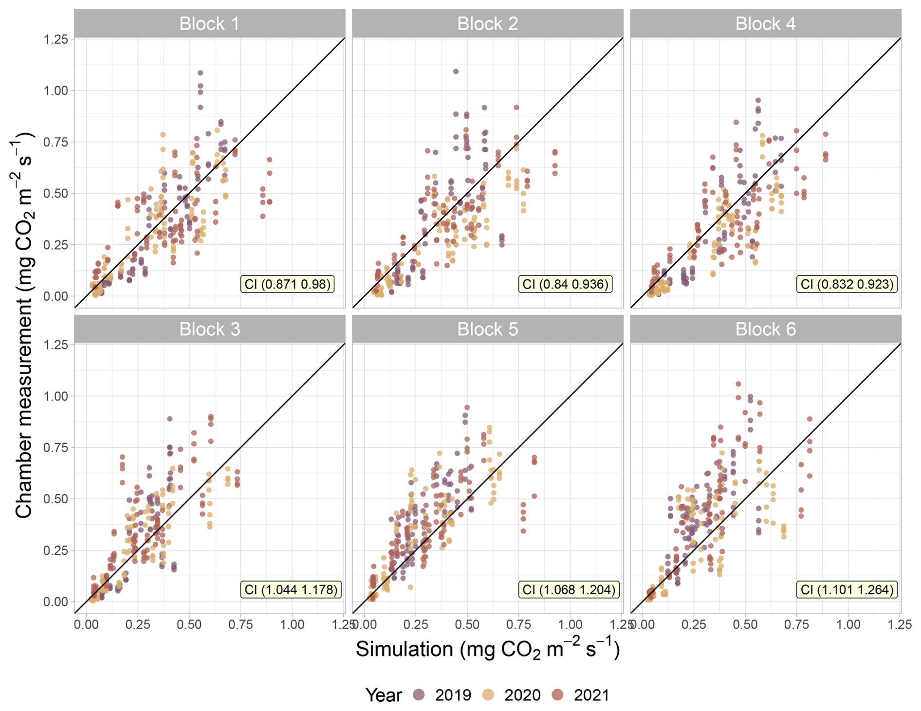
Figure 7 Simulated daily mean and momentarily observed total ecosystem respiration (TER) by chamber measurements in the different blocks in 2019–2021. The confidence intervals (CI) for each regression line slope are stated at the bottom right corners. There were up to four chamber measurements simultaneously at the block, which is reflected in the plot by multiple observations per simulation.

The simulated daily NEE and N₂O fluxes for blocks 5 and 6 followed the seasonal dynamics of the EC observations (Fig. 8). The performance with N₂O fluxes were more variable than with NEE especially in late 2021 and 2022, after the glyphosate applications. The R² values of NEE in blocks 5 and 6 were 0.56 and 0.48, respectively, and for N₂O, 0.086 and 0.003, respectively. Since the EC data did not cover blocks 1–4, comparison with continuous flux data was not possible for any deep peat blocks.

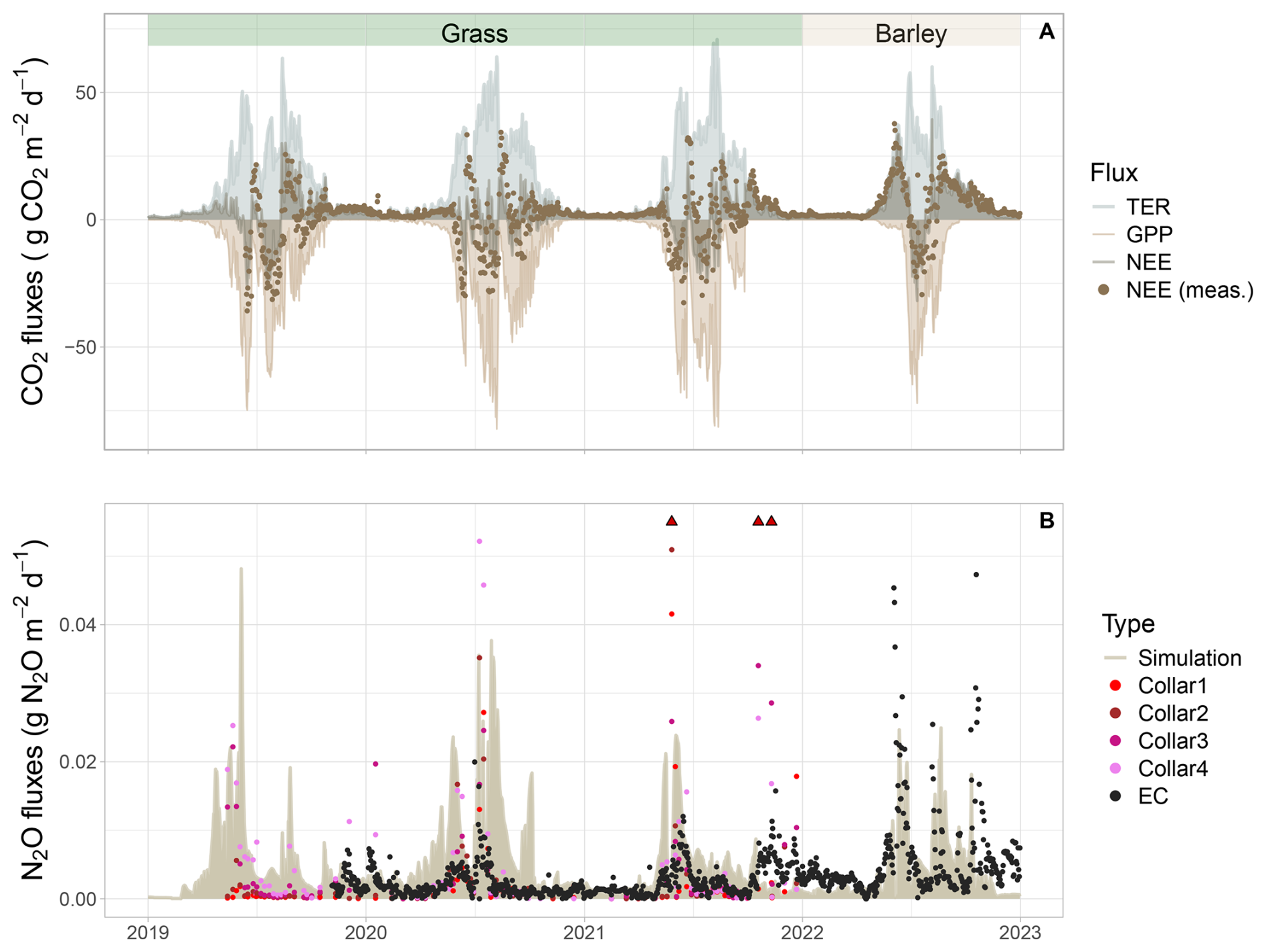
Figure 8 Observed (dots) and simulated (shaded areas) daily (A) net ecosystem exchange of CO₂ (NEE) and (B) N₂O fluxes at the study site from 2019 to 2022. The simulated NEE is divided into gross primary production (GPP) and total ecosystem respiration (TER). Negative values indicate a sink. CO₂ and N₂O fluxes were measured with the eddy covariance (EC) method, but N₂O fluxes were also measured with manual chambers, as indicated by the colored dots (B). The triangles indicate chamber measurements that were outside the scale. These outliers occurred in four instances (two of them stacked) and varied from 0.06 to 0.21 g N₂O m⁻² d⁻¹. Colors at the top of the panel (A) indicate forage grass years (green) and cereal year (beige).

Both the model and EC observations indicated a positive annual NEE for the years 2020–2022, meaning the field was a net source of CO₂. The observed annual NEE balances were 1.06–5.12 t CO₂–C ha⁻¹ yr⁻¹ and the mean simulated balances were 1.29–4.76 t CO₂–C ha⁻¹ yr⁻¹ for blocks 5–6 during 2020–2022, showing a slightly narrower range of variation compared to the measurements. The observed (EC-tower), annual N₂O balances were 4.7–13.0 kg N₂O–N ha⁻¹ yr⁻¹ while the simulated balances for blocks 5 and 6 were (on average) 9.0–15.8 kg N₂O–N ha⁻¹ yr⁻¹. However, even though the ranges overlapped, the simulated balances were generally higher and the interannual variation showed discrepancies between the measured and simulated annual balances. For the shallow peats, the highest N₂O balances were in year 2020 (Table S3), while for measurements, the highest N₂O balance was in year 2022 (Table S4).

3.2 Water table scenarios

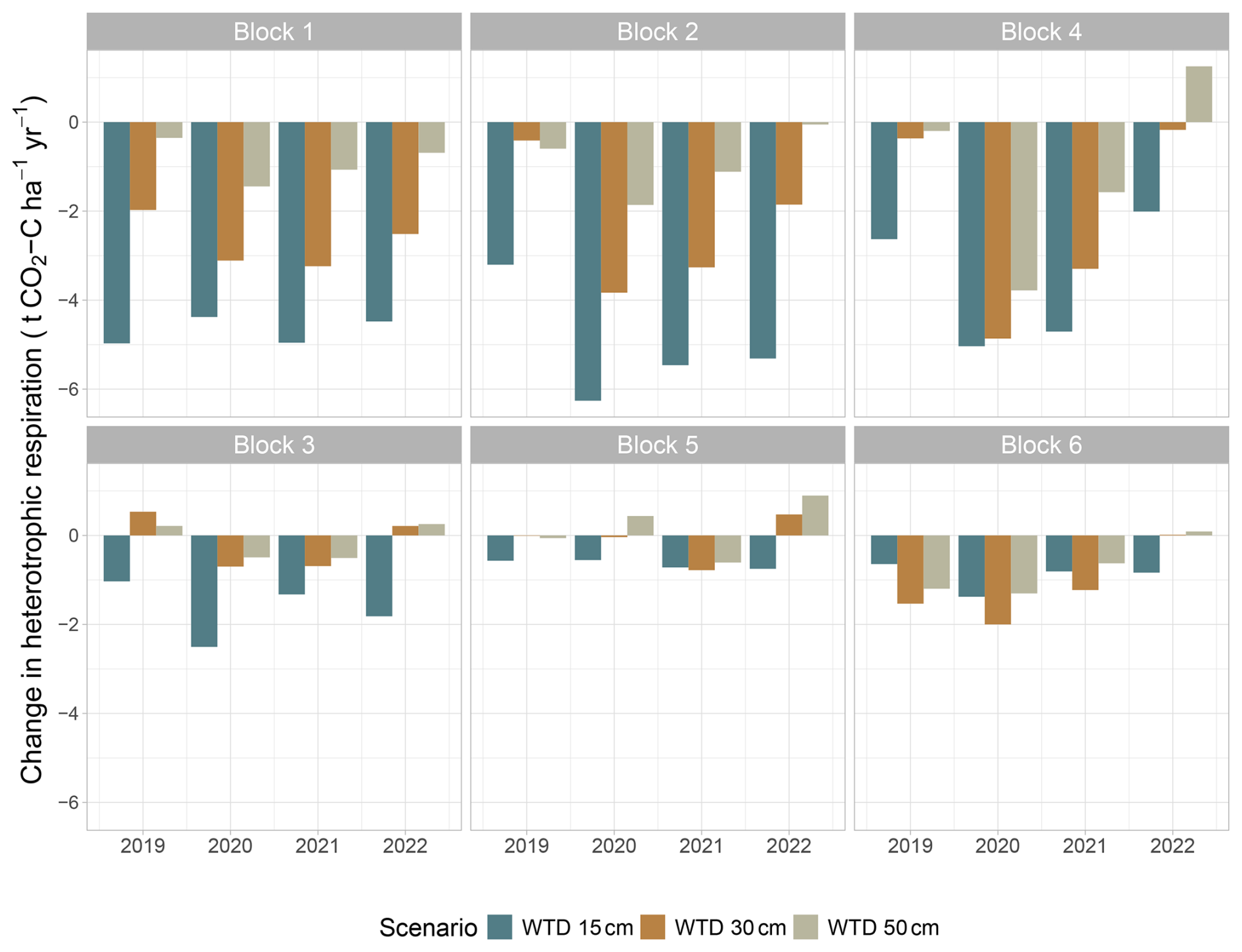
We compared the respiration (auto- and heterotrophic; Ra and Rh) and CO₂ uptake in baseline simulations with the scenarios involving raised WT. The impact of water table raise was notable to Rh, and on average, the increase in the WTD led to decrease in Rh (Fig. 9). There was more mitigation in the deeper peat blocks (1, 2, and 4) than in the shallower ones (3, 5, and 6) when the WT was raised, as on average over the study years, for deep peat blocks, the annual Rh decreased by 1.0 t CO₂–C ha⁻¹ (standard deviation (SD) 1.2) in the 50 cm scenarios, 2.4 t CO₂–C ha⁻¹ (SD 1.5) in the 30 cm scenarios and 4.4 t CO₂–C ha⁻¹ (SD 1.2) in the 15 cm scenarios. The results in shallow peat blocks were on average 0.2 (SD 0.7), 0.5 (SD 0.8) and 1.1 (SD 0.6) t CO₂–C ha⁻¹, respectively. Standard deviations were calculated over the blocks and years. Although Rh mainly decreased with increased WT, all blocks had yearly variation with Rh sometimes increasing compared to the baseline. The changes in Ra and CO₂ uptake were smaller than the changes in Rh. The largest CO₂ uptake changes were seen in 15 cm scenario, where the increases were, on average, 1.1 (SD 1.3) t CO₂–C ha⁻¹ for deep peat blocks and 1.2 (SD 1.0) t CO₂–C ha⁻¹ for shallow peat blocks. However, the net impact for carbon balance was lower as the Ra increased approximately half of the obtained increase in CO₂ uptake.

Figure 9 Changes in the annual heterotrophic respiration in the different blocks and at different water table depth scenarios compared to the baseline scenario. The water table scenarios are introduced in Sect. 2.4.4 and in Fig. 3.

3.2.1 Net ecosystem carbon balance

There was a strong correlation between simulated NECB and exposed OM (i.e organic matter above WTD) (r=0.86), as more organic matter was decomposed in the simulations that had more OM exposed. The simulated NECB values varied due to the different scenarios, variability in species between the years, and soil profile differences among the blocks. In Fig. 10 we have plotted the NECB values in relation to exposed organic matter for the baseline and all scenario simulations, as well as the estimations from measurements. The estimations were based on the NEE from EC and harvest data for years 2020–2022, and combined with the water table and soil properties (Table 1) to obtain organic matter stock above the water table. The overall variability was notable, as the annual NECB values varied from 1.3 to 11.0 t CO₂–C ha⁻¹ yr⁻¹. For the three measured years, approximately 240 t C ha⁻¹ OM remained above the WTD. The NECB values 4.3–6.9 t CO₂–C ha⁻¹ estimated from measurements are in line with the 18 simulated cases with a similar level (230–250 t C ha⁻¹) of exposed OM, as the average NECB in these simulations was 4.7 t CO₂–C ha⁻¹ yr⁻¹ (SD 1.2).

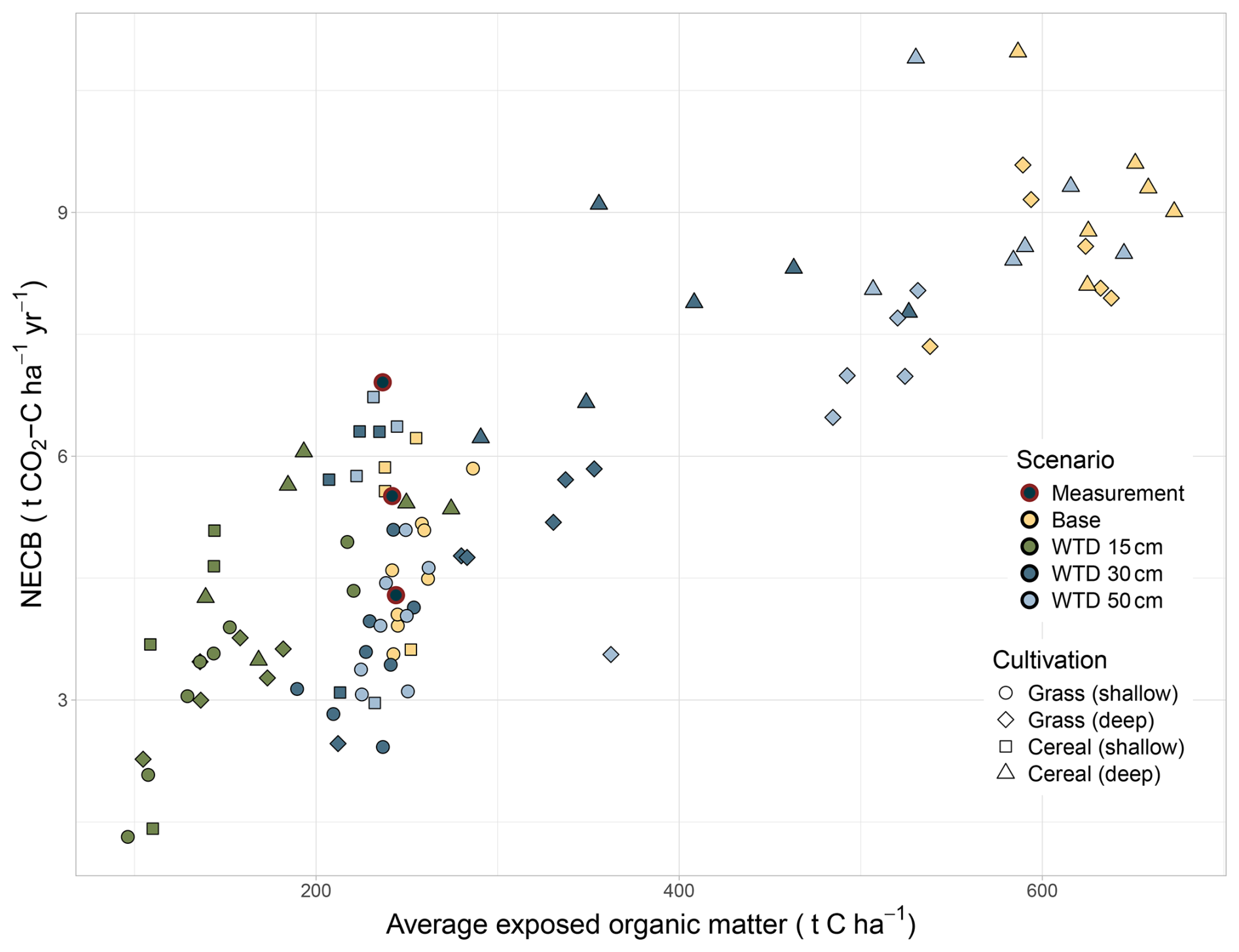
Figure 10 The relationship between exposed organic matter and the annual net carbon balance (NECB) in the different water table scenarios at the different blocks with different peat depths using weather drivers from 2019–2022. The estimates derived from observations are presented as black markers.

3.2.2 N₂O balance

Annual N₂O balances in the baseline runs ranged from 6.4 to 51.7 kg N₂O–N ha⁻¹ yr⁻¹, and on average, the deep peat blocks had larger annual emissions (20.8–35.3 kg N₂O–N ha⁻¹ yr⁻¹ on average in blocks 1, 2, 4) than the shallow peat blocks (10.2–15.4 kg N₂O–N ha⁻¹ yr⁻¹ in blocks 3, 5, 6; Table S3). The annual N₂O balances were also affected by the WTD changes, and on average were reduced by 3.3 kg N₂O–N ha⁻¹ yr⁻¹ (WTD 50 cm), 6.3 kg N₂O–N ha⁻¹ yr⁻¹ (WTD 30 cm) and 10.6 kg N₂O–N ha⁻¹ yr⁻¹ (WTD 15 cm), accounting all of the blocks, in each scenario compared to the baseline.

The average nitrification was 2200 kg N ha⁻¹ yr⁻¹ for deep peat blocks and 1250 kg N ha⁻¹ yr⁻¹ for shallow peat blocks from 2019 to 2022. The annual nitrification was reduced by 16 % (17 %), 35 % (29 %) and 60 % (45 %) in water table scenarios (50, 30 and 15 cm respectively) for deep (shallow) peat blocks.

3.2.3 CO₂ equivalents

The N₂O balances were converted to CO_2 e. and are shown together with the simulated NECB values in Fig. 11. The CO_2 e. balances were highest in the baseline runs and decreased when the WT was raised. In the deep peat blocks, the mitigation effect was stronger (varying on average from 19.6 to 37.6 t CO₂ ha⁻¹ yr⁻¹) than in the shallow peat blocks (varying on average from 15.2 to 20.2 t CO₂ ha⁻¹ yr⁻¹). The average reduction in CO_2 e. differed notably even when expressed relative to the change in water table depth; the largest reduction was obtained in 15 cm scenario (2.3 t CO₂-C ha⁻¹ yr⁻¹) per every 0.1 m water table raise, while 30 and 50 cm scenarios the relative change was notably smaller (1.6 and 1.2 t CO₂-C ha⁻¹ yr⁻¹, respectively). In all WTD scenarios, the share of N₂O in total CO_2 e. balances was consistent (20 %–24 %). However, the proportion of NEE reduced (ranging from 19% to 47 %) while the proportion from the harvest increased (ranging from 29 % to 62 %), although the harvest stayed consistent in absolute terms.

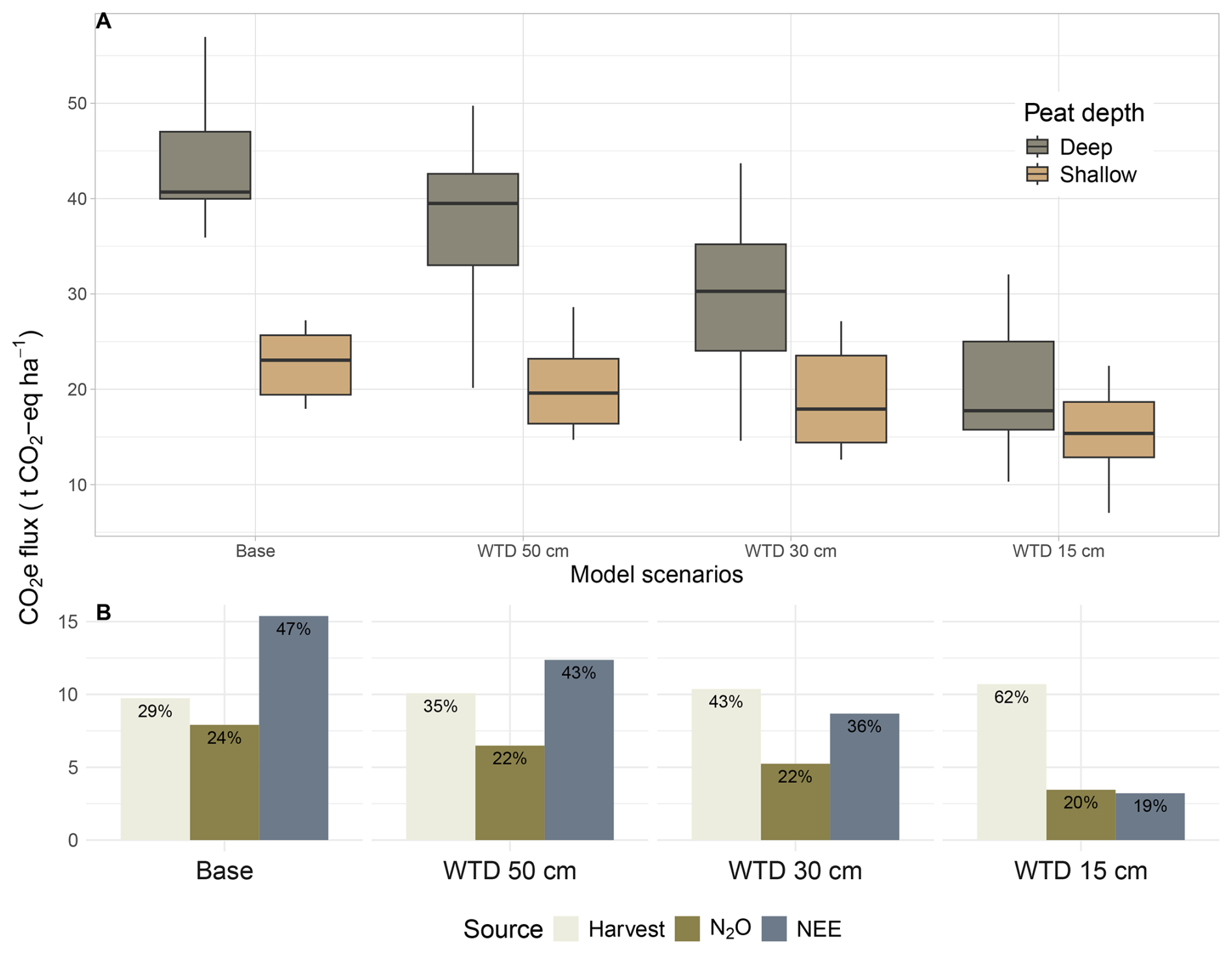
Figure 11 Calculated CO₂ equivalents (CO_2 e.) of the baseline and the water table depth (WTD) scenario simulations with water table raised to a specific depth (on average 15, 30 or 50 cm below the soil surface). The CO_2 e. results are calculated from the annual NECB and N₂O fluxes for years 2019–2022 for each block, with NECB as the sum of net ecosystem exchange (NEE) and the share of carbon from harvest. The results in plot (A) are shown separately for deep peat blocks and shallow peat blocks, while deep and shallow peat blocks are combined in plot (B) to show the average share of CO_2 e. components for each scenario.

3.3 Sensitivity analysis

By varying the decomposition rates (METRX_KR_HUM) in all the original runs, the annual Rh differences ranged from −1.0 to 1.4 t CO₂–C ha⁻¹ yr⁻¹. There was a large variation between the years and the blocks, but on average the largest differences were seen in the scenarios, which had the lowest water table depth i.e. most exposed organic matter. A decrease in decomposition rates of the larger organic matter pools (young and old recalcitrant humus) reduced Rh by 0.3–1.4 t CO₂–C ha⁻¹ yr⁻¹ in deep peat and 0.3–0.9 t CO₂–C ha⁻¹ yr⁻¹ in shallow peat. Conversely, increasing these rates raised Rh by 0.3–1.0 t CO₂–C ha⁻¹ yr⁻¹ in deep peat and 0.2–0.7 t CO₂–C ha⁻¹ yr⁻¹ in shallow peat, depending on the scenario. For the smallest organic matter pool (labile humus), the changes were minor on average, varying only from −0.2 to 0.4 t CO₂–C ha⁻¹ yr⁻¹ as a result of increases and decreases. The aggregated results of annual means and peat depth categories are shown in Fig. 12. The changes in CO₂ uptake and Ra were smaller compared to the changes in Rh, and on average over the years and blocks the CO₂ uptake varied from −0.07 to 0.1 t CO₂–C ha⁻¹ yr⁻¹, while in Ra the variance was even smaller.

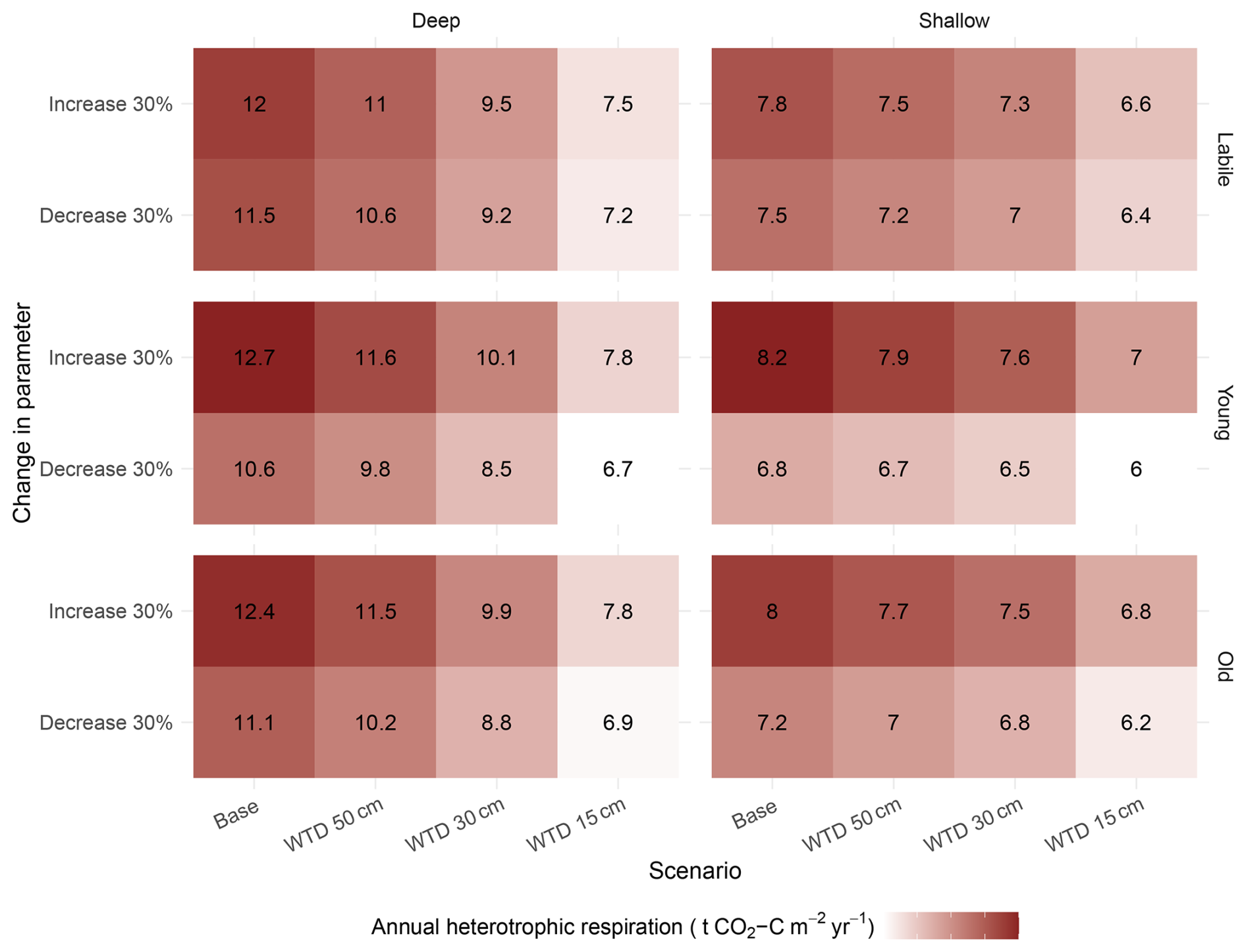
Figure 12 Average annual heterotrophic respiration in each water table depth (WTD) scenario for deep peat blocks and shallow peat blocks after changing decomposition rates. In the baseline run, the annual heterotrophic respiration was 11.8 t CO₂–C ha⁻¹ yr⁻¹ for deep peat blocks, 7.6 t CO₂–C ha⁻¹ yr⁻¹ for shallow peat blocks, and on average 9.7 t CO₂–C ha⁻¹ yr⁻¹ for all blocks.

Changes in the parameter for potential evapotranspiration caused variability in Rh especially in the simulations with lower WTD. For deep peat blocks, a decrease in potential evapotranspiration varied Rh from −0.6 to 1.3 t CO₂–C ha⁻¹ yr⁻¹, while the increase led to changes less than 1 t CO₂–C ha⁻¹ yr⁻¹. In addition, the variability was only seen in the deep peat blocks, while the shallow peat blocks had very minor variability. Similarly, the differences due to the changes in the water use efficiency parameter, which was applied to perennial grasses, were generally small in Rh. On average, lowering or increasing this parameter would have led to only 0.2 t CO₂–C ha⁻¹ yr⁻¹ change in Rh. The averages for shallow and deep peat blocks aggregated over the years can be seen in Fig. S3. Finally, although there was annual variability, and the WTD had a leverage effect on the variability, we saw in the aggregated results that on average the responses to Rh varied in parallel in the base and scenario runs. Therefore, these results indicate that we would have obtained similar outcomes between the base and scenario runs, even if the aforementioned parameter values would have been different. Overall, the emission rates would be distinct, but the effect of raising the water table would still be present.

4 Discussion

4.1 Need for GHG mitigation

Drained agricultural peatlands are known to be hotspots for GHG emissions (Evans et al., 2021; Dinsmore et al., 2009; Gerin et al., 2023), and raising the water table has been proposed as an effective mitigation strategy (Tiemeyer et al., 2016; Freeman et al., 2022). Here, we predict that even a slight increase in the water table could reduce the negative climatic effects of peatland cultivation by decreasing heterotrophic respiration and N₂O emissions, particularly in areas with substantial peat deposits. These results align with studies Heikkinen et al. (2024), Huang et al. (2021b) and Wilson et al. (2016b) that have found the water table depth to be a key driver of CO₂ emissions. On the other hand, studies Leiber-Sauheitl et al. (2014) and Eickenscheidt et al. (2015) challenge the significance of peat depth by demonstrating similar emission rates from soils with different SOC stocks, consistent with studies Bridgham and Richardson (1992); Waddington et al. (2014) indicating that soil respiration would be formed mainly in upper layers. Therefore, it is crucial to evaluate the performance of the model under varying conditions to better understand the effectiveness and limitations of the water table management, and to ensure that management decisions are based on robust, evidence-based assessments.

4.2 Applicability of LDNDC to simulate agricultural peatlands

The model evaluation focused foremost on CO₂ fluxes, which are the major contributor to GHG emissions in peatlands. The simulated daily net ecosystem exchange in the shallow peat field was consistent with the EC measurements (Fig. 8a), which led to a good agreement between the simulated NECB and the estimates derived from the EC and field data (Table S3 and Fig. 10). Similar levels of agreement with observed dynamics were seen in LAI (Fig. 6) as well as soil moisture and evapotranspiration (Figs. 4 and 5). While the in-situ observation and satellite-derived estimates themselves may contain uncertainties, their relative temporal dynamics were captured reliably even though the absolute values remain more uncertain. Altogether, the results supported the conclusion that with suitable parameter modifications (documented in Sect. 2.3.2), the model was capable to simulate crop growth and CO₂ exchange in degraded peat soils with a shallow organic horizon.

On average, the simulated respiration fluxes were in agreement with the chamber measurements from shallow and deep peat fields. However, the model underestimated the ecosystem respiration for the shallow peat fields and overestimated it for deep peat fields.

The N₂O fluxes showed more discrepancies than the CO₂ fluxes, and while the range of annual balances was comparable with the EC measurements, the simulations either under or overestimated the balances by up to a factor of three. By nature, N₂O fluxes are more difficult to simulate because these emissions have typically high temporal variability (Rees et al., 2013) and short-term peak emissions may occur after weather and management events such as freezing-thawing, fertilization or tillage (Rees et al., 2013; Wagner-Riddle et al., 2017; Gerin et al., 2023; Cowan et al., 2025). Even though the simulation captures many of the observed temporal patterns relatively well (Fig. 8b), the missed N₂O episodes especially following the herbicide applications and ploughing led to a poor quantitative agreement on a daily to seasonal level. Ideally, the N cycle part would be calibrated with local data, but the N₂O fluxes alone might not reliably constrain the model: N₂O fluxes make only a small part of total N cycle and result from several processes.

4.3 Water table depth and SOC stock as drivers of GHG emissions

Raising the water table mitigated the simulated GHG emissions in both shallow and deep fields (Fig. 11) with the greatest impact observed for CO₂ emissions. Peat depth and water table depth could be combined for estimating the exposed organic matter stock, which had a strong positive association with the CO₂ emissions (Fig. 10). A similar but weaker relationship was established empirically for cultivated peatlands in the Netherlands by Aben et al. (2024). In the simulations, the change in water table depth mainly affected the heterotrophic respiration, which was reduced even with the more conservative water table changes in this study, where the water table followed the observed seasonal variation and was only moderately higher than the measured water table (Fig. 9).

Similar to the CO₂ emissions, the N₂O emissions were reduced when the water table was raised. Although the comparison against the EC data indicated greater uncertainties in simulating the N₂O emissions compared to the CO₂ fluxes, this result is consistent with several empirical studies (Jeewani et al., 2025; Lång et al., 2024) and supports the hypothesis that increasing the water table can suppress nitrification and subsequently reduce the availability of nitrate for denitrification (Klemedtsson et al., 2005; Pärn et al., 2018). The nitrification reduction was notable in all WT scenarios, and was largest on the highest WT scenario which further supports our latter hypothesis. Cowan et al. (2025) and Liu et al. (2020) do suggest that raising the water table without complete rewetting (WT at soil surface) may lead to similar or higher N₂O emissions due to the higher soil moisture above the WT and near the soil surface, which favors both nitrification and denitrification processes. When raising the WT, the model increases the soil moisture in the layers above the WT, so in theory the model does take into account the potential for similar or higher emissions due to higher soil moisture. In addition, the mitigation effect was still notably weaker than for CO₂ emissions (Fig. 11) and as the amount of carbon removed in harvest did not significantly change, the proportion of N₂O emissions, relative to the total GHG burden, stayed consistent between the scenarios. We note that in the strongly mitigated 30 and 15 cm scenarios, even large increases (+50 %–100 %) in N₂O emissions would not cancel the mitigation from reduced CO₂ emissions. However, additional N₂O measurements over drained agricultural peatlands with raised WT would be very valuable in reducing the model uncertainty and for understanding how the WTD response of N₂O emissions interacts with pedoclimatic conditions.

The model was parametrized primarily based on the data that represented the part of the field with a shallow peat layer, and therefore, the model results for deeper peat profiles involve additional uncertainties. Specifically, our initialization of organic matter pools did not consider differences in chemical properties of the peat layer beyond the carbon and nitrogen contents. Earlier studies, in contrast, suggest that the peat decomposition may be more strongly influenced by other aspects of peat quality, such as its polysaccharide content (Leifeld et al., 2012; Normand et al., 2021), which in turn may vary within the soil profile. The primacy of peat quality as a driver of CO₂ emissions is consistent with previous studies on organic soils where the CO₂ emissions have been found to be decoupled from the C stocks (Leiber-Sauheitl et al., 2014; Eickenscheidt et al., 2015). In addition, the carbon content varied considerably between the soil layers (Table 1) and was relatively low in the topsoil of some blocks, indicating that peat had been mixed with the minerals. A difference in peat quality or mixing of mineral soil with the top peat layers could also explain why the chamber measurements, contrary to the simulations, showed little or no difference in ecosystem respiration between the deep and shallow peat layers.

The model structure also contains simplifications, such as the representation of anaerobic microsites and microbial pathways specific to peat mineralisation. Such structural limitations may partly explain the under – or overestimation observed in some of the simulated respiration, NECB and N₂O fluxes. Altering the decomposition rates was necessary in this study to achieve comparable CO₂ fluxes with the observations. The sensitivity analysis with respect to these parameters indicated that even by varying the key parameters in the model, similar mitigation effects were achieved in CO₂ by raising the water table as with our initial parametrisation. In addition, we varied two parameters related to the water cycle (potential evapotranspiration and water use efficiency). Also these parameter changes had a minor impact on the mitigation potential. This sensitivity analysis showed that our findings regarding the mitigation power were robust to parametrisation, despite the uncertainties in the absolute CO₂ emissions. However, these model experiments cannot assess the uncertainty caused by missing processes or other structural errors. Multi-model simulations, and eventually, empirical studies are needed to further test the accuracy of our predictions.

4.4 Potential to mitigate GHG emissions with water table management

Combining the need to harvest biomass with the need to mitigate emissions creates a strong constraint for cropland management, requiring large changes in agricultural practices and local water management. The largest reduction of GHG emissions was achieved here in the scenario with average 15 cm water table depth, which implies conditions close to those typical in paludiculture. In this case, the net exchange of CO₂ was close to neutral in most of the grass years regardless of the peat layer thickness. However, most of the years with barley still showed high net CO₂ emissions. Seasonal variation of the WTD exposes more soil organic matter to aerobic conditions during the warm season, which is also the most potential time to reduce the CO₂ emissions from soil (Heikkinen et al., 2024). This highlights the need to target water level management during summer months for maximum mitigation.

Nonetheless, the simulations also indicated that small but positive GHG mitigation is possible with less drastic changes to the water table management. The scenario with a 50 cm average WTD required the water table to be raised on average by 31 cm in the deep-peat blocks and by 44 cm in the shallow-peat blocks. This increase in water table level can be achievable with a controlled drainage system and is unlikely to cause issues for conventional agriculture (Salla et al., 2024). In our simulations, this scenario resulted in an annual reduction of GHGs equivalent to approximately 5.8 (deep peat layers) to 2.5 (shallow peat layers) t CO_2 e. ha⁻¹, and in this scenario each 10 cm raise of water table levels reduced annual emission on average by 1.2 t CO_2 e. ha⁻¹. Such a change in long-term average WTD is sufficient for modest mitigation in emissions (Evans et al., 2021; Lång et al., 2024). Somewhat surprisingly, the emissions were reduced even in the simulations with the average WTD very close to or below the organic soil horizon in the shallow peat blocks (Table 1). However, due to the seasonal variation and the way how counterfactual water tables were constructed, the peat layers were submerged more frequently and for longer periods in the scenario runs than in simulations with observed WTD (Fig. 3). On average raising the WT reduced CO₂ emissions throughout the year, but largest CO₂ emissions were seen at the end of the growing season. At this time of year the water table level is typically lower than at the beginning of the growing season and would not reach the peat layer. However, in the scenario runs, the peat layer was usually partially submerged. As the controlled drainage offers multiple benefits, such as reduced nutrient leaching (Carstensen et al., 2020) and increase in available water for plants (de Wit et al., 2022), a minor climate benefit is a worthwhile addition if conversion to a more climate-neutral land use is not possible.

The water table scenarios used in the simulations were not tied to any specific water management practices, such as ditch blocking, controlled drainage or subsurface irrigation. While we evaluated the mitigation potential related to peat depth under idealized scenarios, in practice, GHG mitigation efforts are limited by local climate, hydrogeology, and drainage management practices (Boonman et al., 2022). Ideally, these aspects would be incorporated into the model structure to establish the site-specific mitigation potential.

5 Conclusions

Raising the water table was found to be an effective way of reducing emissions even in shallow peat fields. Overall, the simulation results showed a clear association between the stock of exposed organic matter and CO₂ emissions, indicating that even moderate changes to water management practices can help to mitigate greenhouse gas emissions. We found that the LDNDC model could be adapted to simulate agricultural peatlands, and a sensitivity analysis indicated that the estimated mitigation effect achieved by raising of water table was robust to changes in the parameters governing evapotranspiration and organic matter decomposition. Future work is still needed to simulate N₂O fluxes as accurately as CO₂ emissions, particularly given its high sensitivity to environmental conditions. Additionally, the model was parameterized and evaluated mainly using data representing a shallow peat layer, and future studies should be conducted to understand relationship between GHG emissions and the peat layer thickness on a more mechanistic level. The results indicate that well-drained peat soils that still retain a high carbon stock should be targeted to effectively mitigate climate change. Yet, the results also suggest that smaller reductions in annual emissions are possible in cultivated peatlands with thinned peat deposits, even with conservative changes to the water management practices.