Drivers of ecosystem stability differ with the intensity of extreme climatic events

This study investigates how the dominant predictors of Normalized Difference Vegetation Index (NDVI) based vegetation stability metrics vary across gradients of hydroclimatic extremity. While previous studies have documented the impacts of droughts and heavy rainfall on ecosystem functioning and resilience inferred from stochastic fluctuations, less attention has been given to whether the relative importance of climatic, biodiversity-related, and landscape predictors changes systematically under different levels of climatic stress. To address this question, we quantified vegetation resistance and resilience responses and compared the contributions of meteorological variables, modeled anthropogenic species-change proxies and topographic factors across a global range of hydroclimatic conditions. We find that under normal to moderately dry conditions, vegetation stability metrics are primarily associated with meteorological variables, particularly temperature and precipitation, consistent with earlier global assessments. Under severe and extreme drought conditions, resistance decreases markedly across most regions, whereas resilience responses exhibit weaker and more spatially heterogeneous changes. Importantly, in sparsely vegetated ecosystems such as grasslands and open shrublands, the relative importance of leading predictors shifts from climatic to non-climatic variables under intensified drought stress, suggesting context-dependent associations with vegetation stability. Deciduous needle-leaf forests show consistently low resistance and resilience values across climatic regimes, suggesting elevated sensitivity to hydroclimatic variability. Overall, our findings suggest that vegetation stability under climatic extremes cannot be fully explained by meteorological forcing alone and that these modeled proxies and landscape heterogeneity provide additional predictive information under intensifying climate variability.

1 Introduction

Ecosystem stability refers to the capacity of ecological systems to maintain and recover their functional integrity when exposed to environmental disturbances (Holling, 1973). Resistance and resilience, representing the degree to which ecosystems withstand perturbations and the extent of recovery following disturbance relative to normal climatic conditions, respectively, remain foundational metrics for understanding ecological responses to ongoing global environmental change (Van Meerbeek et al., 2021). These concepts provide a common framework for quantifying how ecosystems respond to and recover from external shocks. As climate change intensifies, extreme events such as severe droughts and heavy rainfall are becoming more frequent and severe (Ripple et al., 2024), increasing the need to assess resistance and resilience as key indicators of ecological vulnerability (Sun et al., 2022).

Recent advances in satellite remote sensing have enabled global assessments of vegetation stability across diverse ecosystems. Global-scale analyses using the Normalized Difference Vegetation Index (NDVI) time series have shown that vegetation sensitivity to climatic variability is widespread, with many ecosystems responding strongly to changes in water availability and temperature (Seddon et al., 2016). Additional work has demonstrated that resistance and resilience tend to be lower in regions experiencing substantial anthropogenic disturbance (Li et al., 2018). Other global studies have reported that evergreen broadleaf forests maintain particularly high ecosystem stability, with species diversity contributing significantly to ecosystem stability in combination with radiation and temperature (Huang and Xia, 2019). More integrative modeling indicates that ecosystem stability emerges through interactions among climatic conditions, biodiversity, soil properties, and vegetation structural attributes, rather than through any single driver (Chen et al., 2021).

In parallel, recent global assessments of vegetation resilience have increasingly focused on intrinsic system stability inferred from stochastic fluctuations and autoregressive memory structures (Forzieri et al., 2022; Smith et al., 2022; Smith and Boers, 2023). While these approaches provide valuable insights into long-term stability dynamics, they primarily quantify system-level memory effects rather than resilience responses to discrete hydroclimatic events. In contrast, the present study quantifies event-scale resistance and resilience dynamics associated with explicitly defined climatic extremes. Because our primary focus is on nonlinear ecosystem responses to discrete hydroclimatic perturbations – such as droughts and excessive rainfall – we adopt an event-conditioned evaluation framework that does not explicitly parameterize autoregressive processes, while recognizing that legacy and memory effects remain embedded in ecosystem states and observed responses.

Collectively, these studies highlight the multifactorial nature of ecosystem stability, but they share several important limitations. First, most previous global assessments have not evaluated how the dominant predictors of stability change across different intensities of climatic extremes. Analyses typically evaluate stability under average or static climatic contexts, without distinguishing between normal, moderate, and severe-to-extreme drought and wet conditions. This represents a critical gap, because ecosystems often exhibit nonlinear or threshold-type responses under extreme climatic stresses that differ fundamentally from responses observed under normal climatic conditions. Such nonlinear responses have been hypothesized in ecological theory, where ecosystems may remain relatively stable up to a critical stress level and then shift rapidly once that threshold is exceeded (e.g., alternative stable states and ecological thresholds frameworks). In addition, empirical and conceptual research suggests that variation in species-level responses to environmental change – so-called response diversity – is a key determinant of how ecological communities respond to increasing stress, and the loss of such response diversity can lead to abrupt declines in ecosystem resilience rather than gradual changes (Mori et al., 2013). For example, this previous research provides a conceptual model showing that when species vary in their sensitivity to stressors, community-level functions can be maintained until compensatory dynamics break down, potentially resulting in threshold-like system responses. These findings highlight the importance of considering nonlinear and threshold dynamics when evaluating ecosystem stability across climatic extremes.

Second, key non-climatic contributors, such as biodiversity, soil properties, and land-use history, have rarely been integrated comprehensively. Land management intensity has been shown to modify biodiversity–resilience relationships, with positive effects emerging only under the strongest management regimes, whereas drought resistance has been associated more strongly with mowing frequency than with species richness (Vogel et al., 2012). Long-term land-use history has been linked to variation in resistance through its influence on plant functional traits (Adler et al., 2004). Soil conditions, including moisture, carbon content, and bulk density, have also been identified as important but underexplored determinants of stability (Berdugo et al., 2022; Wei et al., 2025). In addition, topographic factors such as elevation, slope, and aspect regulate microclimatic conditions, soil water redistribution, and solar radiation, thereby modulating vegetation exposure and sensitivity to climatic extremes. These terrain-driven controls can amplify or buffer drought and heat stress at local scales, yet they are often overlooked in large-scale assessments of ecosystem resistance and resilience.

Despite these findings, no previous global analysis has simultaneously incorporated climatic variables, modeled biodiversity -related metrics, anthropogenic species gains and losses, soil properties, topographic factors, and land-use histories within a unified framework. Equally important, no prior study has examined whether – and how – the relative importance of these predictive importance changes systematically with the severity of climatic extremes, such as those defined by the Standardized Precipitation–Evapotranspiration Index (SPEI). Consequently, predictions of ecological vulnerability under future climate scenarios remain limited.

To address these gaps, the present study investigates how the dominant predictors of vegetation resistance and resilience vary across a full gradient of drought and wetness severity categories. Using satellite-derived NDVI data, hydroclimatic characterization based on SPEI, and a machine-learning approach (LightGBM), the present study evaluates the relative contributions of climatic variables, modeled anthropogenic species-change proxies (including anthropogenic species increases and losses), soil properties, elevation, irrigation intensity, and long-term land-use histories across diverse land-cover types and hydroclimatic regimes.

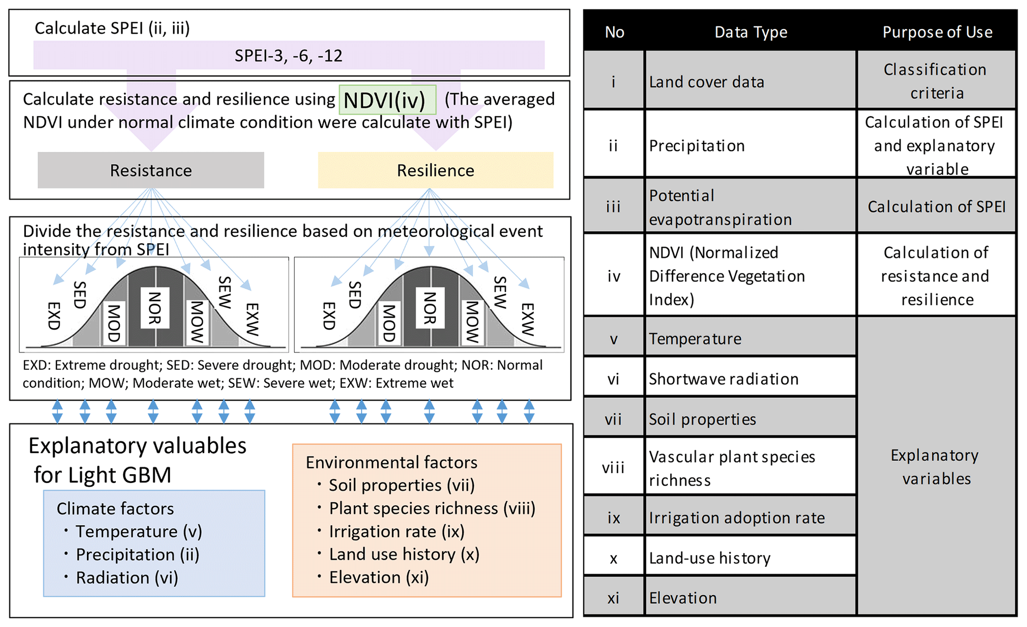
Figure 1 Left: Analytical workflow illustrating the processing steps applied after all grid cells were first classified by land-cover type, with subsequent analyses conducted separately for each land-cover class. The left panel also shows the use of SPEI at 3-, 6-, and 12-month accumulation time scales (SPEI-3, SPEI-6, and SPEI-12), representing short-term, seasonal, and annual water-balance conditions, respectively. Right: Datasets and their roles in the analysis. Roman numerals in the left panel correspond to the items listed on the right. Item i (land-cover data) is not shown in the left panel because land-cover classification was performed as a prerequisite step, and all subsequent analyses were conducted independently within each land-cover category. In total, the modeling framework encompassed multiple combinations of land-cover types, climatic time scales, climate-event classes, and response metrics. Specifically, resistance and resilience were calculated for 11 land-cover classes, three SPEI accumulation time scales (SPEI-3, SPEI-6, and SPEI-12), and seven climate-event categories defined separately for each SPEI time scale. As both resistance and resilience were evaluated for each combination, this design resulted in 11 × 3 × 7 × 2 = 462 individual models, all of which were analyzed to assess ecosystem responses to climatic extremes.

This integrated approach allows us to evaluate whether the dominant predictors of NDVI-based vegetation stability differ between moderate and extreme climatic conditions, including meteorological variables, modeled anthropogenic species-change proxies, and structural variables. By explicitly stratifying analyses across multiple climate-extreme categories and incorporating a uniquely comprehensive set of explanatory factors, this study provides a new multidimensional perspective on how ecosystems respond to increasingly frequent and intense climatic extremes.

Our findings offer an improved and more comprehensive predictive understanding of global patterns of ecological vulnerability and have important implications for designing climate-specific and ecosystem-specific management and conservation strategies aimed at sustaining ecosystem functioning in an era of accelerating climate change. Throughout this study, resistance and resilience refer to NDVI-based, event-scale indices of proximity to normal-year vegetation activity, rather than comprehensive mechanistic measures of ecosystem stability.

2 Materials and Methods

2.1 Overview of the Analytical Workflow and Spatiotemporal Scales

Global datasets harmonized to a 5 arcmin (0.0833°×0.0833°) spatial grid were first divided by land-cover type and then assigned to climate event classes. Figure 1 (left) outlines the workflow for land-cover classification, and Fig. 1 (right) summarizes the datasets and their functions. The datasets used in the analysis were divided into three groups: (1) those used to derive the response variables (resistance and resilience), (2) those used to compute explanatory variables, and (3) those used for classification (land cover and SPEI).

All datasets were harmonized to a 5 arcmin spatial resolution. Time-series analyses were conducted over the period 1982–2015, excluding 1990–1994. NDVI during this interval was influenced by NOAA-11 orbital drift, which shifted the satellite's equatorial crossing time by ∼ 3.7 h (Li and Brown, 2017) and altered the solar geometry during acquisition. This period also included the Pinatubo eruption, thereby introducing additional radiative anomalies. To avoid these confounding effects, NDVI data for 1990–1994 were removed, and all analyses were conducted for 1982–1989 and 1995–2015. As NDVI quality declines at high latitudes, the analysis domain was restricted to 60° N–60° S (Beck et al., 2006; Justice et al., 1985).

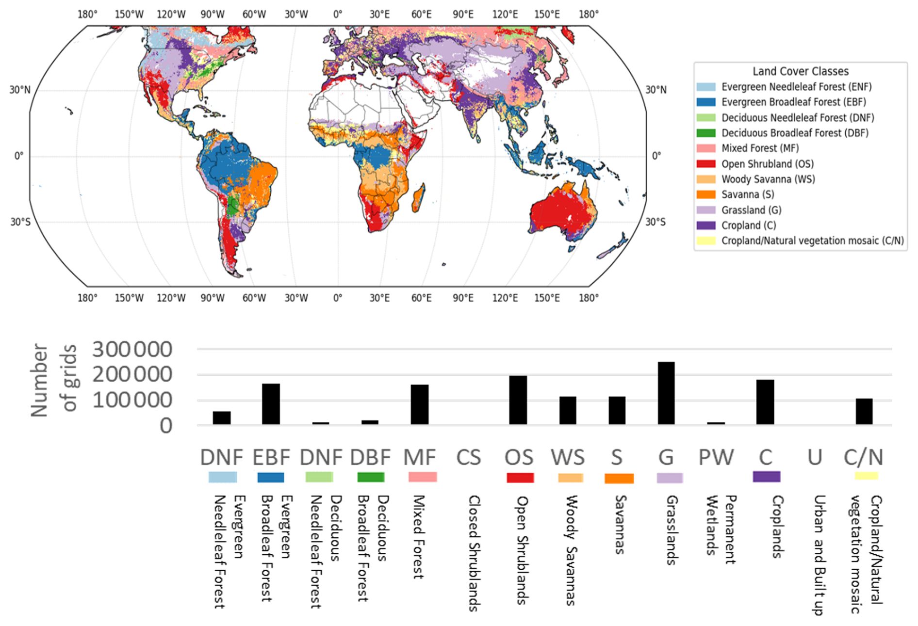
Figure 2 Spatial distribution of each land-cover type (upper figure) and the corresponding number of grid cells (lower graph). The lower bar chart represents the total number of grid cells for each land-cover type. Among them, CS, PW, and U were excluded from the analysis because the number of grids in these categories was extremely small. In addition, although not shown here, Barren areas – regions with almost no vegetation – were also excluded from the analysis. On the global map, only the land-cover types included in the analysis are color-coded.

2.2 Site Selection

Terrestrial regions worldwide were included, except for land-cover types represented by very few grid cells (Channan et al., 2014). The excluded classes were Closed Shrublands (CS), Permanent Wetlands (PW), Urban and Built-up areas (U), Barren land (B), and Snow and Ice (SI). The retained land-cover classes included Evergreen Needleleaf Forest (ENF), Evergreen Broadleaf Forest (EBF), Deciduous Needleleaf Forest (DNF), Deciduous Broadleaf Forest (DBF), Mixed Forest (MF), Open Shrublands (OS), Woody Savannas (WS), Savannas (S), Grasslands (G), Croplands (C), and Cropland/Natural Vegetation Mosaic (C/N). Land-cover data were used at a 5 min spatial resolution.

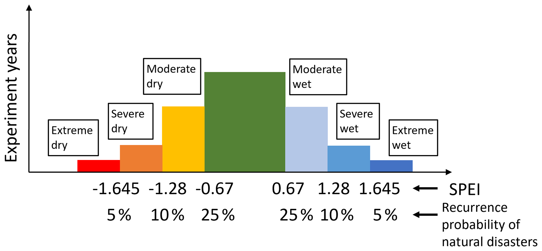
Figure 3 Classification of seven climate conditions based on SPEI. SPEI is an index derived from a probability distribution, meaning that its values correspond directly to probabilities under a standard normal distribution. An absolute value of 1.645 represents a 5 % probability level. In this study, we classified climatic conditions with absolute SPEI values greater than 1.645 as extreme events, which occur with a probability of less than 5 %, or roughly once every 20 years. Similarly, climatic conditions with absolute SPEI values between 1.28 and 1.645 correspond to a 5 %–10 % probability range and were classified as severe events. Conditions with absolute values between 0.67 and 1.28 correspond to a 10 %–25 % probability range and were classified as Moderate events. All remaining values were categorized as Normal conditions, which occur with a probability of approximately 50 %, representing climatic conditions that are expected to occur roughly once every 2 years.

2.3 Classification of Climate Conditions

The climate conditions for each grid cell were classified using the Standardized Precipitation–Evapotranspiration Index (SPEI, Vicente-Serrano et al., 2010) at 3-, 6-, and 12-month time scales for 1982–2015. Seven categories were defined (Fig. 3): extremely dry (SPEI < −1.645), severely dry (SPEI < −1.28), moderately dry (SPEI < −0.67), normal (−0.67 ≤ SPEI ≤ 0.67), moderately wet (SPEI > 0.67), severely wet (SPEI > 1.28), and extremely wet (SPEI > 1.645). These thresholds correspond to the probabilities under a standard normal distribution.

SPEI was computed using the SPEI R package (Begueria and Vicente-Serrano, 2017) using precipitation from GPCC v7.0 (1° resolution; Schneider, 2015) and potential evapotranspiration from CRU-TS 4.01 (0.5° resolution; University of East Anglia Climatic Research Unit et al., 2017). To obtain complete time series across all SPEI scales, climate data from 1981 to 2015 were used. SPEI results were then aligned with the NDVI datasets after the removal of 1990–1994.

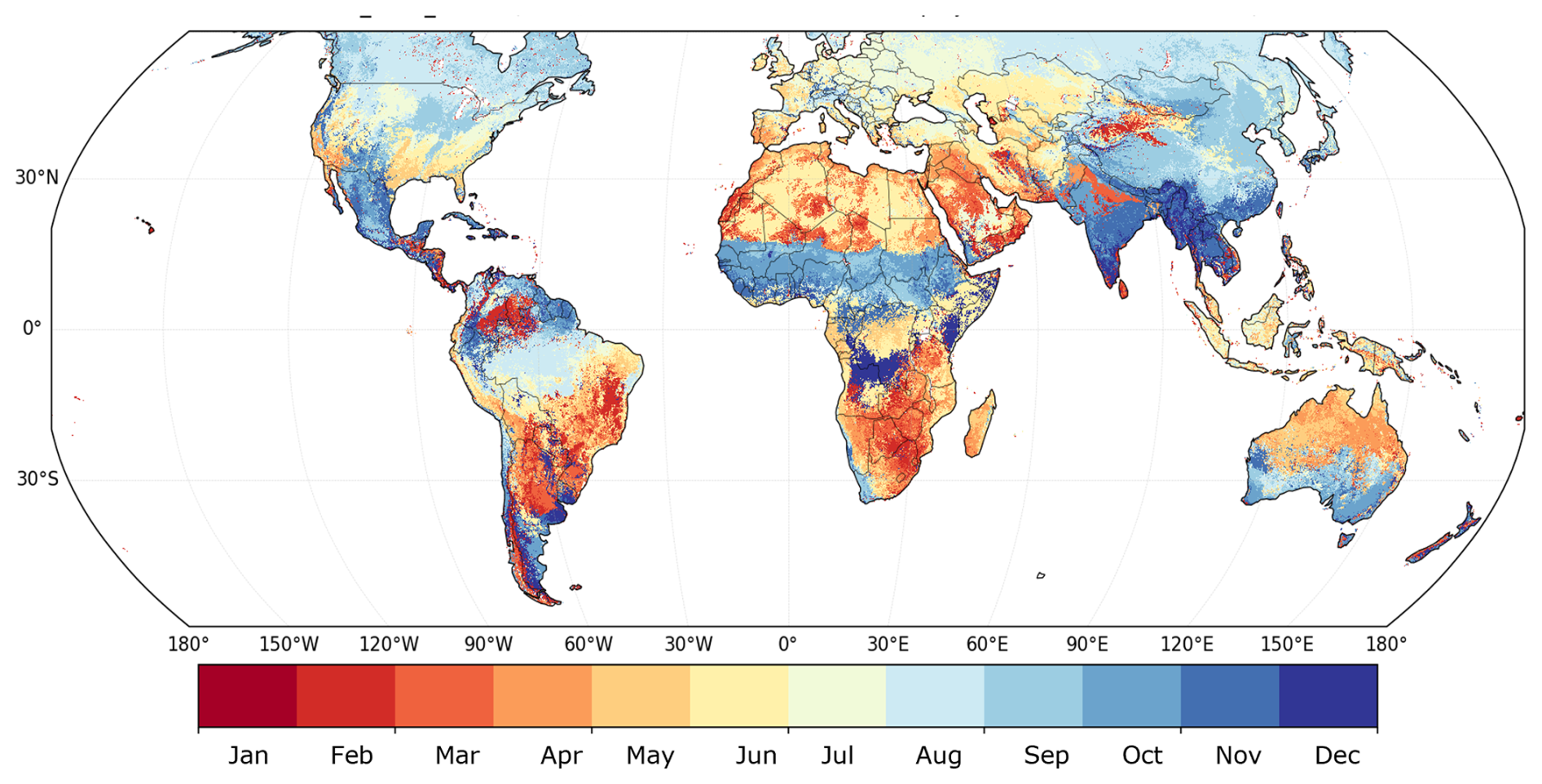
Figure 4 The month detected for each grid. The Detected Month represents the month in which the annual maximum NDVI most frequently occurred during the analysis period for each grid cell. Specifically, for each year, the month with the highest monthly NDVI was identified, and the frequency of these peak-NDVI months was counted across all years. The month with the highest occurrence was then assigned to each grid cell. The figure shows these results using a color-coded scheme, where the numbers 1–12 correspond to the calendar months.

2.4 Calculation of Resistance and Resilience

Resistance and resilience were derived from the NDVI3g dataset (GIMMS; Pinzon and Tucker, 2014) at a 5 arcmin resolution. NDVI from 1990 to 1994 was excluded. The maximum biweekly NDVI value was retained for each month. For each grid cell, the month that most frequently contained the annual NDVI maximum between 1982 and 1989 and between 1995 and 2015 was identified (Fig. 4). This “peak month” was treated as a proxy for annual vegetation productivity.

In this study, resistance and resilience were defined as event-based proximity indices to the normal-year vegetation condition. Resistance quantifies how close vegetation activity during the climate-event year was to the normal-year level, whereas resilience quantifies how close vegetation activity in the year following the event was to the normal-year level. These indices were calculated as follows:

$$\begin{array}{}\text{(1)}& {\displaystyle }& {\displaystyle }\text{Resistance}={\displaystyle \frac{\mathrm{1}}{\left({\text{NDVI}}_{\mathrm{m}}-{\text{NDVI}}_{\mathrm{e}}\right)+\mathrm{1}}}\text{(2)}& {\displaystyle }& {\displaystyle }\text{Resilience}={\displaystyle \frac{\mathrm{1}}{\left({\text{NDVI}}_{\mathrm{m}}-{\text{NDVI}}_{\mathrm{e}+\mathrm{1}}\right)+\mathrm{1}}}\end{array}$$

where NDVI_m  is the mean NDVI in normal years (−0.67 ≤ SPEI < 0.67), NDVI_e is the NDVI during the climate-event year, and NDVI_e+1 is the NDVI in the year after the event.

Under this formulation, a value of 1 indicates vegetation activity comparable to the normal-year condition. Values below 1 indicate reduced vegetation activity relative to normal years, whereas values above 1 indicate above-normal vegetation activity. Thus, the indices are centered around 1 and provide a direct interpretation as proximity to normal vegetation activity. This property is useful for global pixel-wise mapping, land-cover comparisons, and machine-learning analyses because the same reference value can be used across pixels, event categories, and land-cover types.

We adopted this formulation because the objective of this study was to compare global vegetation responses across land-cover types and hydroclimatic-event categories using response variables with a direct and consistent interpretation. Alternative stability metrics emphasize different aspects of disturbance response. For example, ratio-based metrics such as the Isbell-type formulation can become extremely large or undefined when the event-year or post-event vegetation index is very close to the normal-year condition (Isbell et al., 2015). Bounded metrics such as the Orwin and Wardle-type formulation are useful for evaluating departure from a control condition, but above-normal vegetation activity is treated as a deviation from the normal state rather than as enhanced vegetation activity (Orwin and Wardle 2004; Liu et al., 2022). Log-response metrics are useful for quantifying proportional change, but they are centered around 0 and do not directly indicate whether vegetation activity has returned to the normal-year condition (Xu et al., 2022; Yan et al., 2025).

Therefore, our indices should be interpreted as proximity-to-normal vegetation activity indices, rather than as direct substitutes for all previously proposed resistance and resilience metrics. To clarify the behavior of our metrics relative to commonly used alternatives, we provide numerical comparisons with Isbell-type, Orwin and Wardle-type, and log-response formulations in Tables S1 and S2 in the Supplement. These comparisons show how each metric responds when vegetation activity is equal to the normal condition, declines below it, recovers to it, or exceeds it.

Autoregressive formulations were not used because the analysis incorporated categorical and non-time-series explanatory variables.

NDVI was used rather than EVI because the main objective of this study was to analyze resistance and resilience over a long temporal period and to capture as many extreme dry and wet events as possible. The GIMMS NDVI3g dataset provides a globally consistent vegetation record beginning in 1982, whereas a directly comparable long-term EVI product is not available for the full study period. Because EVI requires spectral bands that are not available from the AVHRR-based GIMMS NDVI3g record, an EVI-based analysis could not be conducted over the same temporal extent.

We acknowledge that EVI has important advantages over NDVI, including reduced saturation in high-biomass vegetation and improved correction for soil and atmospheric background effects. Therefore, the use of NDVI may affect the estimated magnitude of resistance and resilience, particularly in dense forests, sparsely vegetated systems, and regions where soil background effects are important. To evaluate this limitation, we conducted an additional MODIS-based comparison using both NDVI and EVI over the same period and added the results to the Supplement (Figs. S2 and S3). This comparison was used as a sensitivity analysis to assess how the choice of vegetation index may influence the estimated resistance and resilience values.

Table 1 Explanatory variables used in the LightGBM analysis

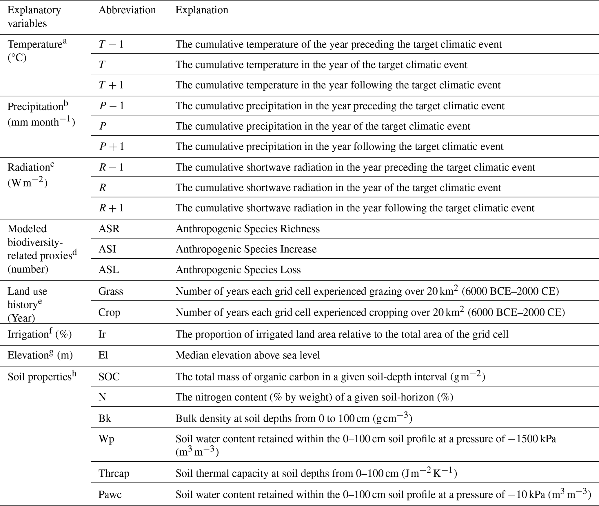
Note. All time-series datasets were analyzed for the target periods of 1982–1989 and 1995–2015, and were resampled to a uniform spatial resolution of 5 min. Although the original datasets were provided in different physical units, all variables were normalized to a common 0–1 range prior to analysis to ensure comparability among predictors.
^a University of East Anglia Climatic Research et al. (2017). ^b Schneider et al. (2015).^c European Centre for Medium-Range Weather Forecasts (2012).^d Ellis et al. (2012). ^e Klein Goldewijk et al. (2011). ^f Siebert et al. (2013). ^g Fischer et al. (2008). ^h Global Soil Data Task Group (2000).

2.5 Explanatory Factors

Twenty-two explanatory variables were compiled and grouped into four categories: climatic, abiotic, biodiversity-related, and land-use history/irrigation variables (Table 1 and Supplement).

Climatic Factors: Annual precipitation (P: Schneider, 2015), temperature (T: University of East Anglia Climatic Research Unit et al., 2017), and shortwave radiation (R: European Centre for Medium-Range Weather Forecasts, 2012) were obtained for the event year, the preceding year (−1), and the following year (+1). The +1 variables were used only for resilience models, yielding 19 explanatory variables for resistance and 22 for resilience models.

Abiotic Factors: Elevation (Fischer et al., 2008) and six soil properties (Global Soil Data Task Group, 2000) – bulk density, wilting point, plant-available water capacity, thermal capacity, soil organic carbon, and soil nitrogen – were included because of their roles in water and nutrient regulation.

Biodiversity-Related Factors (Ellis et al., 2012): Anthropogenic species increase (ASI) was estimated using alien species distributions, crop species data, and urban area extent. Anthropogenic species loss (ASL) was derived from vegetation patterns and habitat-based models. Anthropogenic species richness (ASR) was calculated as follows:

$$\begin{array}{}\text{(3)}& \text{ASR}=N-\text{ASL}+\text{ASI}\end{array}$$

where N is the potential species richness, estimated using the global model by Kreft and Jetz (2007). These variables are modeled biodiversity-related proxy variables and should not be interpreted as direct observations of local biodiversity change.

Land-Use History and Irrigation: HYDE 3.1 data (Klein Goldewijk et al., 2011) were used to estimate the duration (years) that each grid cell had been under cropland or pastureland for the past 8000 years. The extent of irrigation was obtained from the Global Map of Irrigation Areas (Siebert et al., 2013).

2.6 Normalization of Explanatory Variables

Non–time-series variables (soil, elevation, land-use history, ASR/ASI/ASL) were normalized to a 0–1 scale using the global minimum and maximum values:

$$\begin{array}{}\text{(4)}& Y={\displaystyle \frac{X-X_{min}}{X_{\text{Max}}-X_{\text{Min}}}}\end{array}$$

X: Data for any given grid

Y: Normalized data (0–1 range) for the corresponding grid

X_Max: Maximum value across all grids

X_Min: Minimum value across all grids

Time-series climatic variables (T, P, R) were aggregated to annual values and normalized within each grid cell across 1982–1989 and 1995–2015 as follows:

$$\begin{array}{}\text{(5)}& Y_i={\displaystyle \frac{P_i-P_{min}}{P_{\text{Max}}-P_{\text{Min}}}}\end{array}$$

P_i: Data for year i

Y_i: Normalized data (0–1 range) for year i

P_Max: Maximum value across all years

P_Min: Minimum value across all years

Grids outside 60° N–60° S were excluded because of NDVI reliability limitations.

2.7 Modeling Approach

The relationship between the explanatory variables and vegetation resistance or resilience was assessed using a Light Gradient Boosting Machine (LightGBM) model (Shi et al., 2025). LightGBM was selected because it can efficiently capture nonlinear relationships and interaction effects among multiple climatic, edaphic, topographic, biodiversity-related, and land-use predictors without requiring a priori assumptions about functional forms, which is particularly important for ecosystem–climate analyses where threshold behavior and scale-dependent responses are common. In addition, its histogram-based learning algorithm and leaf-wise tree growth strategy enable high computational efficiency, making it well suited for large-scale, high-dimensional environmental datasets.

Another advantage of LightGBM is its robustness to multicollinearity among predictors, such as correlated climate variables or indices at different accumulation time scales, allowing all explanatory variables to be retained without prior dimensionality reduction. Furthermore, LightGBM can internally handle missing values by learning optimal split directions for missing observations, which reduces the need for explicit gap-filling procedures and improves robustness when working with long-term remote-sensing and climate datasets. In the present analysis, however, rows containing missing or infinite values were removed before model fitting to ensure consistent input data across repeated model runs.

For each model configuration, the data were randomly divided into training and testing datasets using an $\mathrm{80}/\mathrm{20}$ split. The models were trained with up to 500 boosting iterations, and early stopping was applied if the prediction accuracy did not improve for 50 consecutive iterations. Model performance was evaluated using the root mean square error (RMSE), mean absolute error (MAE), and coefficient of determination (R²). These settings follow the attached robustness scripts, in which TEST_SIZE = 0.20, NUM_BOOST_ROUND = 500, and EARLY_STOPPING_ROUNDS = 50 were used.

To quantify the relative contribution of individual explanatory variables, feature importance was evaluated using the gain metric:

$$\begin{array}{}\text{(6)}& {\text{Feature\hspace{0.17em}\hspace{0.17em}Importance\hspace{0.17em}\hspace{0.17em}(Gain)}}_j={\sum }_{t\in T_j}\mathrm{\Delta }{\text{Loss}}_t\end{array}$$

where T_j denotes the set of decision tree splits that involve feature j, and ΔLoss_t represents the reduction in the loss function attributed to split t. Because this metric directly reflects the degree to which each variable contributes to reducing the model error, it is a practical and interpretable indicator of variable influence in gradient boosting models. In each model run, gain-based feature importance was calculated for all predictors, normalized by the total gain, and the top five predictors were retained for the robustness summary.

To assess the robustness of the LightGBM results, we repeated the model training under multiple random seeds, tree-structure hyperparameter settings, and learning-rate settings. Learning rate is also a hyperparameter in LightGBM; here, we treated it separately from the two tree-structure parameter settings in order to explicitly evaluate sensitivity to the step size of boosting updates. For each learning-rate setting, we used three random seeds and two tree-structure hyperparameter settings, resulting in six independent model runs per model configuration. The three random seeds were 0, 1, and 2. The two tree-structure parameter settings were an original setting and a simpler-tree setting. The original setting used num_leaves = 23, min_data_in_leaf = 1, feature_fraction = 1.0, bagging_fraction = 1.0, bagging_freq = 0, and max_depth = −1. The simpler-tree setting used num_leaves = 15, min_data_in_leaf = 20, feature_fraction = 0.9, bagging_fraction = 0.9, bagging_freq = 1, and max_depth = 6.

We further evaluated the sensitivity of the results to the learning-rate hyperparameter by repeating this six-run procedure under three learning-rate settings: 0.1, 0.2, and 0.3. This procedure was applied to all 462 model configurations, defined by the combination of three SPEI timescales, 11 land-cover types, seven event categories, and two response variables. Thus, each model configuration was evaluated using 18 runs in total, resulting in 8316 model runs across all configurations.

For each learning-rate setting, we summarized the six runs and identified the variable that most consistently showed the highest gain-based importance. We then compared the selected top variables across the three learning-rate settings and adopted the variable that was most frequently selected as the dominant predictor. If the same variable was selected under all three learning-rate settings, it was regarded as a robust top predictor. If the same variable was selected under two of the three learning-rate settings, the result was marked with a triangle symbol to indicate moderate robustness. If different variables were selected under all three learning-rate settings, the result was recorded as “nan,” indicating that no single dominant predictor was consistently identified.

This repeated-modeling procedure was used to reduce the dependence of feature-importance interpretation on a single random seed, tree-structure hyperparameter setting, or learning rate, and to provide a more systematic assessment of uncertainty in the selected top predictors.

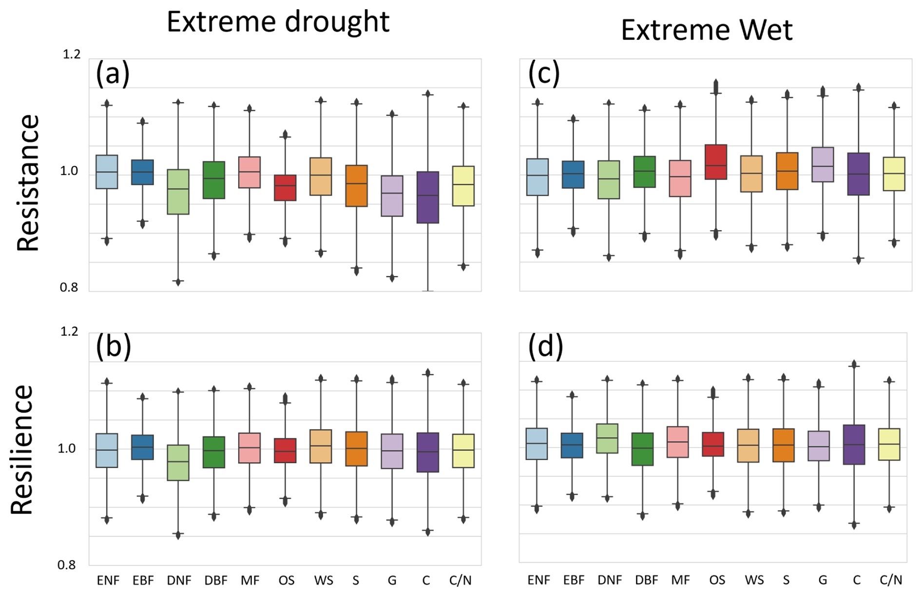
Figure 5 Boxplots of vegetation resistance and resilience for each land cover type under different SPEI-3 climate categories. For each land cover class, resistance values were aggregated across grid cells and filtered by removing statistical outliers based on the interquartile range (IQR; values outside Q1 − 1.5 × IQR and Q3 + 1.5 × IQR were removed). For visualization, the values were restricted to the range of 0.8–1.2. The box edges represent the 25th and 75th percentiles, the center line indicates the median, and the whiskers extend to the most extreme non-outlier values.

3 Results

3.1 Variation in Vegetation Resistance and Resilience with SPEI Severity of Extreme Events

Figure 5 shows the resistance and resilience estimated from SPEI-3, separated by climatic conditions, with results for extreme drought and extreme wet conditions across all land cover types. To improve the readability of the displayed distributions, the y-axis range in Fig. 5 was restricted to 0.8–1.2. However, values outside this range accounted for only a very small proportion of the data: 0.418 % for SPEI-3, 0.417 % for SPEI-6, and 0.412 % for SPEI-12. Thus, most resistance and resilience values were distributed within the 0.8–1.2 range (Table S3 in the Supplement).

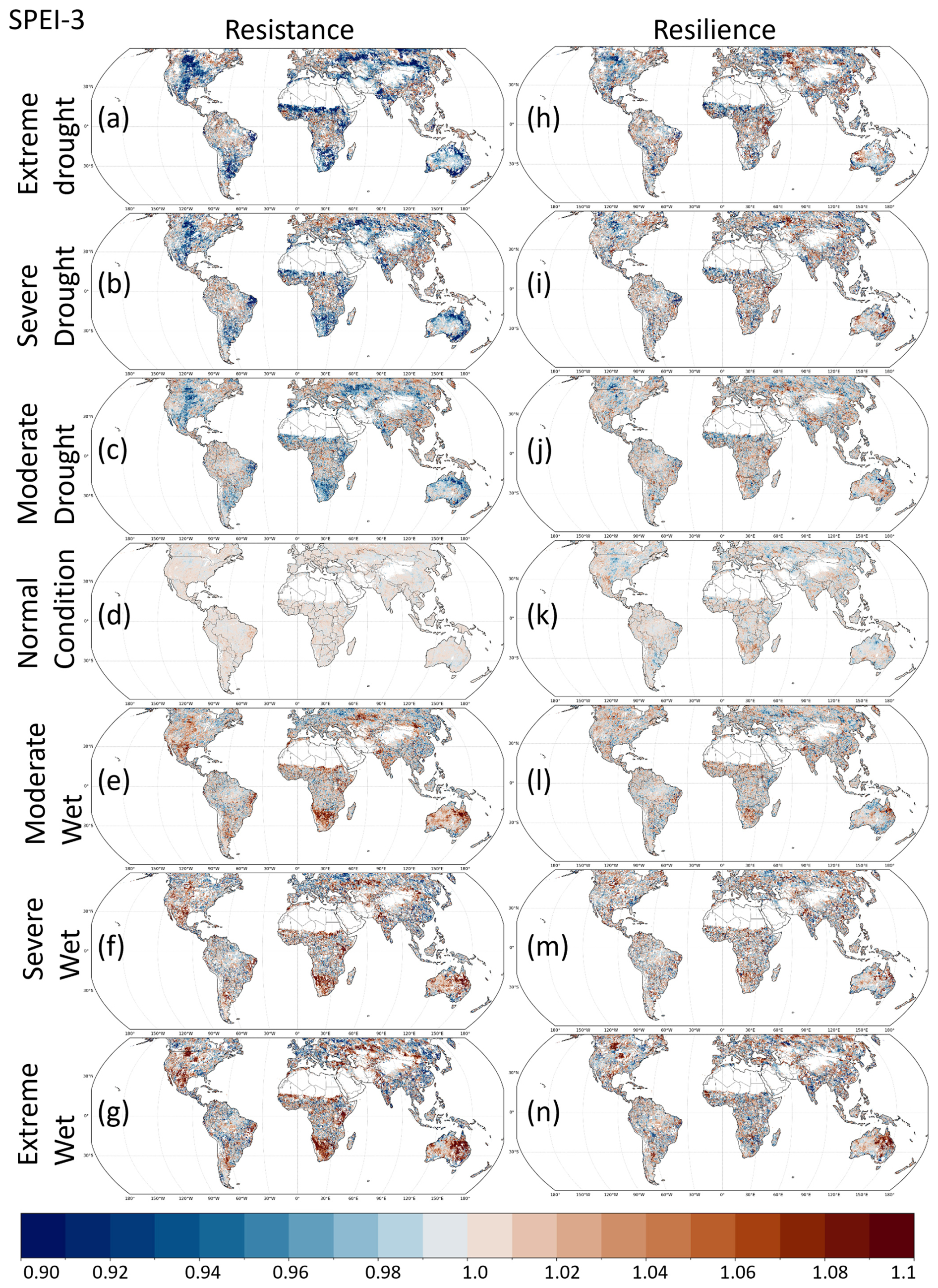
Figure 6 Spatial distribution of resistance and resilience under seven climate categories based on SPEI-3. Vegetation resistance and resilience were calculated using GIMMS NDVI3g data for 1982–1989 and 1995–2015. The normal years required for these calculations were identified using the 3-month SPEI. Climate categories (Extreme, Severe, Moderate, Normal) were defined so that Extreme wet/dry events occur in about 5 % of years, Severe events occurred in approximately 10 % of the years, and moderate events occurred in approximately 25 % of the years; all remaining years were classified as normal.

Figure 6 shows the spatial distribution of resistance and resilience based on SPEI-3 for all climate categories. The full set of results for all SPEI timescales and climatic conditions is presented in Fig. S4 in the Supplement.

In Fig. 5, the median values indicate that, under both drought and wet conditions, deciduous needle-leaf forests (DNF) exhibit low resistance and low resilience under extreme drought conditions. Open shrublands (OS), grasslands (G), and croplands (C) also showed resistance and resilience values below 1 under extreme drought conditions, similar to DNF, but their resilience values were not as low as those of DNF.

Drought-related patterns in Fig. 6a and b show that resistance declines most strongly in dryland regions, especially in areas classified as grasslands (light purple) and savannas (orange) in Fig. 2. These regions include sub-Saharan Africa, the interior of the Eurasian continent, and the central Great Plains of North America, where resistance markedly decreases. Reductions in resilience were weaker and less spatially coherent than those in resistance. Under wet conditions, partial decreases in resistance appear in some high-latitude and temperate regions. By stratifying resistance and resilience according to the climate category, the maps revealed that ecosystem responses to extreme events vary strongly among regions (Fig. 6), underscoring the need to compare ecosystem stability under comparable climatic conditions rather than assuming spatially uniform responses.

Table 2 Variables with the highest feature importance in the LightGBM analysis for each climate–land cover combination.

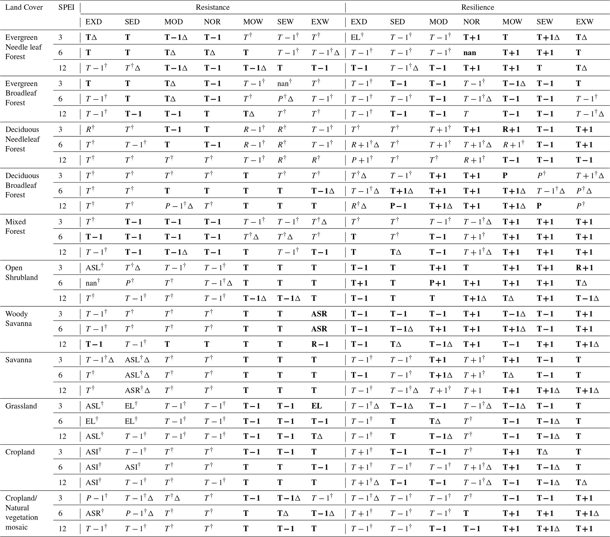
Note. Each string represents an explanatory variable listed in Table 1. Values lower than 1 are indicated by the dagger symbol (†), whereas values equal to or greater than 1 are shown in bold. If the same variable was selected under two of the three learning-rate settings, the result was marked with a triangle symbol to indicate moderate robustness. If different variables were selected under all three learning-rate settings, the result was recorded as “nan,” indicating that no single dominant predictor was consistently identified.
T, P, and R denote temperature, precipitation, and shortwave radiation, respectively. The suffix −1 refers to the year preceding the climate event, and +1 refers to the year following the event. El is the elevation, ASR is the anthropogenic species richness, ASI is the anthropogenic species increase, and ASL is the anthropogenic species loss.

3.2 Drivers of Resistance and Resilience Identified by LightGBM

For each of the 11 land-cover types, the most important variables in the LightGBM models for resistance and resilience were identified across three SPEI time scales (3, 6, and 12 months) and seven water-balance categories (Table 2). In total, 462 (11 × 2 × 3 × 7) model configurations were evaluated. Values below 1.00 are indicated by a dagger symbol (†), whereas values equal to or greater than 1.00 are shown in bold.

The analysis was stratified by SPEI time scale, land-cover type, climatic event category, and response variable. The feature importance of each explanatory variable in the LightGBM models for resistance and resilience was summarized for each land-cover type and climate category (Tables S4 and S5 in the Supplement).

To assess the robustness of model performance, six model runs were treated as one set, and this procedure was repeated three times using different learning-rate settings. Across these three sets of analyses, the model that consistently showed the highest R² was the SPEI-3 model for resistance under extreme drought in DNF, with an R² of 0.717. In contrast, the model that consistently showed the lowest R² was the SPEI-6 model for resistance under normal conditions in EBF, with an R² of 0.097. Because each set included 462 model results, a total of 1386 model-performance records were generated. These results are provided through the link included in the Supplement.

3.3 Drivers under Normal Climate Conditions

Under Normal climatic conditions, temperature-related variables were consistently identified as the leading predictors of ecosystem stability, with the exception of resilience in DNF under SPEI-12, for which R+1 had the highest importance. For resistance, the temperature in the event year (T) was the most frequently selected driver, appearing in 18 of the 33 combinations (≈ 54.5 %). For resilience, the temperature in the post-event year (T+1) was selected in 18 combinations (≈ 54.5 %).

These patterns indicate that temperature-related variables were the leading predictors of NDVI-based vegetation stability metrics under normal conditions. The temporal shift in the selected temperature predictors is consistent with the definitions of the two indices: resistance, which represents proximity to normal vegetation activity during the event year, was more strongly associated with event-year temperature, whereas resilience, which represents proximity to normal vegetation activity in the year following the event, was more strongly associated with post-event temperature.

3.4 Leading Predictors across Hydroclimatic-Event Classes

For ENF, EBF, DNF, DBF, and MF, across these forest-dominated land cover types, climate variables were consistently identified as leading predictors, with temperature most frequently showing the highest gain-based importance. As shown in Table 2, DNF often showed temperature or radiation as the variable with the highest feature importance, whereas DBF frequently showed both temperature and precipitation among the top-ranked drivers. These feature-importance patterns suggest that climatic variables provide substantial predictive information for NDVI-based resistance and resilience in forest systems, with radiation showing high predictive importance in DNF and precipitation showing relatively high importance in DBF.

The effects of drought on OS, S, G, C, and C/N were especially pronounced under severe and extreme drought conditions. Under Severe or Extreme droughts, non-climatic variables – ASI, ASL, ASR, and elevation – often emerged as the highest feature importance rather than climate variables. These land cover types share relatively sparse or structurally constrained vegetation, which may limit their buffering capacity against water stress.

In OS and G, ASL had the highest feature importance under extreme drought at the SPEI-3 timescale, and resistance values were below 1. In C, ASI was selected as the leading predictor under extreme drought (Table 2), suggesting an association between modeled anthropogenic species-increase proxies and NDVI-based stability in croplands. In C/N, ASR showed the highest contribution to resistance under SPEI-6.

Under Extreme or Severe wet conditions, both resistance and resilience exceeded 1 in these sparsely vegetated or managed land cover types, indicating enhanced vegetation functioning. In such cases, temperature-related variables are the most frequently identified leading drivers. ASR was the most influential variable for WS resilience under SPEI-3 and SPEI-6, and elevation showed the highest feature importance for G resistance under SPEI-3.

4 Discussion

4.1 Variability Characteristics of Resistance and Resilience

Our results revealed that vegetation resistance declines markedly during droughts, particularly in arid and semi-arid regions (OS, S, G), whereas resilience exhibits weaker and less spatially coherent declines. Deciduous needle-leaf forests (DNF) consistently show low resistance and resilience, indicating high sensitivity to hydroclimatic variability. This finding is consistent with previous studies reporting reduced ecosystem stability or increased ecosystem degradation in DNF under drought and precipitation variability (Hai et al., 2025; Li et al., 2021; Nogovitcyn et al., 2023). Regions where both stability components are low are likely to experience heightened ecological vulnerability, as reduced resistance and resilience imply a diminished capacity to withstand and recover from climatic disturbances (Yao et al., 2024). Accordingly, our findings suggest that DNF may become increasingly vulnerable under future climate change scenarios.

Sparse vegetation systems, such as open shrublands (OS), grasslands (G), and croplands (C), also exhibit low resistance but maintain comparatively high resilience (Fig. 5b and d). Mapping stability across climatic categories demonstrates substantial spatial heterogeneity in ecosystem responses, highlighting that ecosystems do not respond uniformly to droughts or heavy rainfall. Even under similar climatic conditions and within the same land-cover type, resistance and resilience responses to extreme climatic events can vary markedly. This spatial heterogeneity is consistent with previous findings that sparse vegetation, although highly vulnerable to immediate drought impacts, often exhibits rapid post-drought recovery (Ponce-Campos et al., 2013; Seddon et al., 2016). The pronounced spatial heterogeneity observed in this study underscores the necessity of evaluating ecosystem stability within comparable climatic contexts rather than generalizing responses across biomes or land cover types.

4.2 Feature Importance of Resistance and Resilience Across Climatic Gradients

Temperature-related variables were identified as leading predictors of both resistance and resilience under normal climatic conditions. Although this result partially overlaps with the findings of Huang and Xia (2019), a direct comparison is difficult because the climatic gradient classifications differ. The high predictive importance of temperature-related variables is consistent with studies reporting temperature-driven vegetation shifts and abrupt transitions in ecosystem functioning (Berdugo et al. 2022). Resistance was most strongly associated with temperature in the event year (T) in forest-type land-cover areas. This pattern is consistent with Vitasse et al. (2019), who showed that late spring frost can substantially reduce current-year growth in forest tree species, indicating that temperature anomalies during the event year may be associated with changes in growth-related resistance. At the same time, antecedent temperature may also be important, given the concept that ecosystems undergo “pre-conditioning” through prior thermal and soil moisture conditions before extreme events (De Keersmaecker et al., 2015; Fu et al., 2024). Thus, resistance may reflect both the direct impact of event-year temperature and the legacy effects of climatic conditions in the preceding year.

Resilience, defined here as proximity to normal vegetation activity in the year following the event, was most strongly associated with temperature in the year after the extreme event (T+1). One major reason for this is likely that the resilience metric explicitly incorporates NDVI in the year following the event. In addition, although this interpretation remains hypothetical, the result may partly reflect the temperature sensitivity of root and shoot regrowth processes during post-disturbance recovery (Wu et al., 2025). Taken together, these findings suggest that the timing of temperature-related predictors differ between resistance and resilience. However, because this study considered only a one-year window before and after each extreme event, longer-term evaluations are needed to better capture ecosystem-specific response times and delayed recovery processes.

Under Severe and Extreme drought conditions, non-climatic variables, particularly modeled anthropogenic species increase (ASI), anthropogenic species loss (ASL), anthropogenic species richness (ASR), and elevation, frequently emerged as dominant predictors in sparsely vegetated areas. This pattern suggests that these variables provide additional predictive information when water availability is extremely limited. In such environments, even small changes in species composition or vegetation structure may be associated with differences in resistance and resilience to severe climatic stress. This predictive pattern is broadly consistent with previous research linking higher biodiversity to enhanced ecosystem stability under extreme climatic events (Isbell et al., 2015), but modeled anthropogenic species-loss proxies should be interpreted as predictive associations rather than direct evidence of increased vulnerability in sparse vegetation systems. The study by Isbell et al. (2015) was based primarily on grassland data from Europe and North America in the Northern Hemisphere, and therefore does not provide direct support for the global-scale patterns observed in the present study. In addition, the biodiversity-related variables used here may have been influenced more strongly by relatively recent land-cover conditions than by the long-term land-use history considered in this study. Thus, the apparent importance of ASI, ASL, and ASR should be interpreted as an indication of potential biodiversity-related effects rather than as direct evidence of causal mechanisms.

Taken together, the results indicate that more detailed monitoring and analysis are needed in sparsely vegetated regions, where small changes in vegetation structure and species composition may strongly affect ecosystem stability under severe drought. Furthermore, as shown in Fig. S2, the comparison between EVI and NDVI indicates relatively large differences between the two vegetation indices in OS and G. This suggests that the choice of vegetation index may affect the patterns observed in sparsely vegetated areas. To enhance the robustness of such interpretations, future analyses should incorporate multiple vegetation indices where possible. In the present study, however, NDVI was selected because its long-term availability enabled us to include the largest possible number of extreme events within the analysis period.

In croplands, ASI emerged as the most important variable under Extreme drought conditions. This result may suggest that management-dependent species turnover, such as changes in crop varieties or cultivated species composition, can influence resistance during drought events. This interpretation is broadly consistent with agronomic studies showing that cultivar selection can play an important role in modulating crop productivity and stability under drought conditions (Lobell et al., 2014). Collectively, these results point to a possible interaction between climatic and biotic factors and suggest that species composition and land management practices should be considered when assessing ecosystem stability.

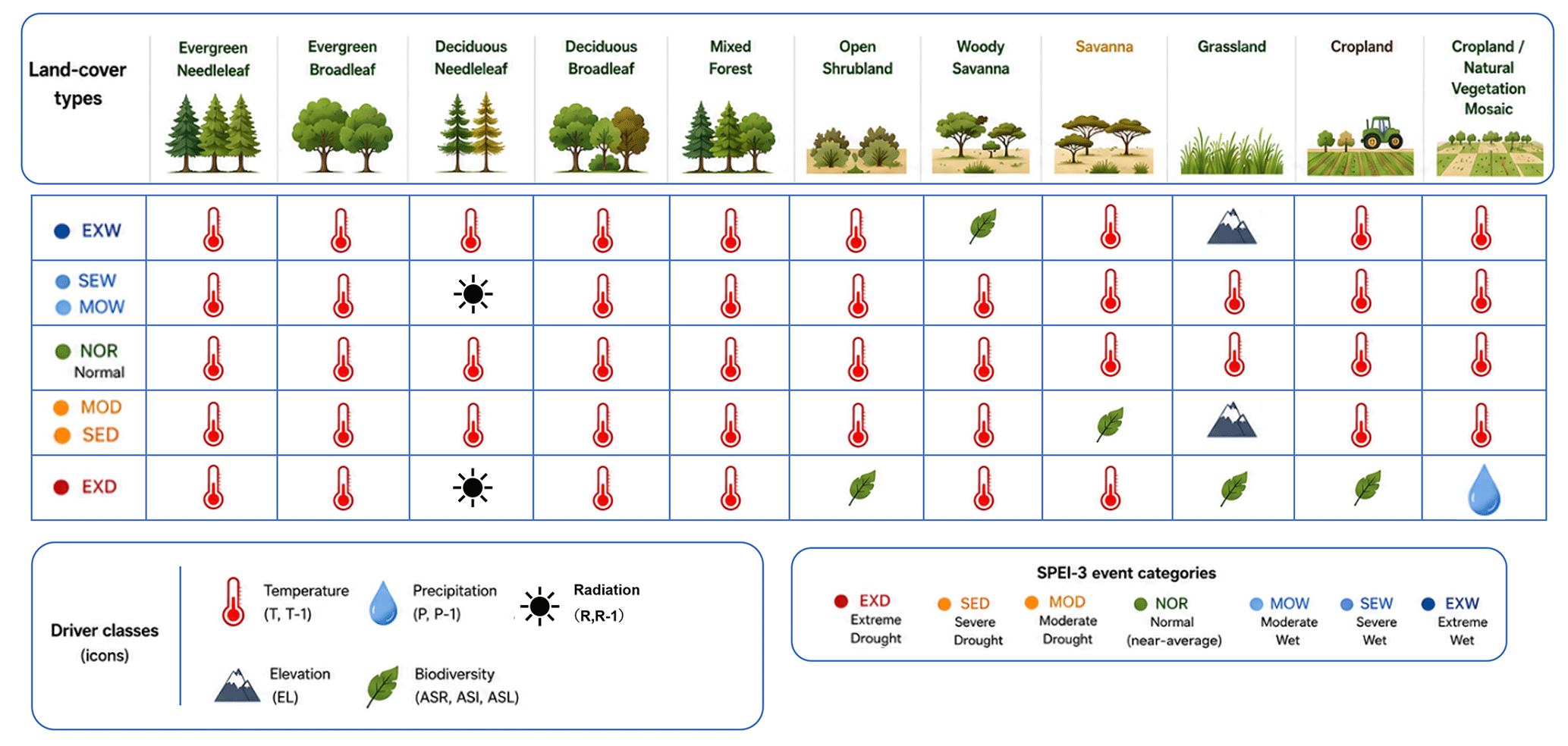
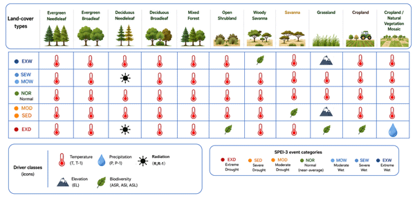
Figure 7 Synthesis diagram showing climate-gradient-dependent drivers of resistance under SPEI-3 drought conditions.

Overall, the results indicate that ecosystem stability shifts substantially along the climatic severity gradient. Under Normal conditions, temperature-related variables were frequently selected as leading predictors of both resistance and resilience. Under severe and extreme droughts, the relative predictive importance of climatic variables decreased in several sparsely vegetated systems, whereas non-climatic variables, including modeled anthropogenic species-change proxies and elevation, showed increased predictive importance for vegetation stability metrics (Fig. 7). These findings demonstrate that climatic variables alone are insufficient for predicting vegetation stability under intense water limitation and that ecological and structural traits must be incorporated into the predictive frameworks.

4.3 Limitations

Despite the strengths of this study, several limitations should be acknowledged. First, the temporal discontinuity caused by excluding NDVI observations from 1990 to 1994 may have reduced the continuity of long-term trends. However, this exclusion was necessary to avoid potential artifacts associated with NOAA-11 orbital drift and the eruption of Mt. Pinatubo.

Second, the biodiversity-related indicators used in this study, namely anthropogenic species increase (ASI), anthropogenic species loss (ASL), and anthropogenic species richness (ASR), as well as the long-term land-use reconstruction dataset HYDE 3.1, are based on modeled estimates and therefore contain inherent uncertainties. These uncertainties may have influenced the relative importance of explanatory variables estimated by the models. More specifically, ASI and ASL are model-based indicators of anthropogenic species gains and losses estimated by Ellis et al. (2012), using native vascular plant species richness (N) derived from Kreft and Jetz (2007) as a baseline. ASL was estimated mainly from habitat loss using species–area relationships, whereas ASI was calculated as the sum of species increases associated with exotic species invasions, crop species, and ornamental plants. Therefore, these variables should not be interpreted as direct differences between observed and predicted current species richness. Rather, they should be regarded as modeled indicators representing potential anthropogenic changes in plant species richness.

Third, LightGBM identifies statistical associations rather than causal mechanisms. Although the present analysis used a large global dataset, spatial autocorrelation among grid cells may still have affected model performance and the estimated importance of explanatory variables. Therefore, the identified drivers should be interpreted as variables statistically associated with resistance and resilience, rather than as direct causal factors.

Fourth, relying solely on NDVI as a proxy for vegetation functioning may underestimate productivity changes in high-biomass ecosystems because of canopy saturation. To address this concern, we compared the results based on NDVI and EVI and presented these comparisons in Figs. S2 and S3 in the Supplement. Nevertheless, the choice of vegetation index may still influence the observed patterns, particularly in ecosystems where vegetation signals are weak or where index-specific sensitivities differ.

Fifth, climatic variables were aggregated at the calendar-year scale. This may introduce uncertainty in regions with pronounced wet–dry seasonality, because the use of calendar years can artificially split wet or dry seasons across different years. As a result, climate signals relevant to ecosystem responses may be weakened or distorted. This issue is particularly important in monsoonal and seasonally dry ecosystems, where ecological responses are often closely linked to seasonal water availability.

Finally, the resistance and resilience metrics used in this study represent only part of the broader concept of ecosystem stability. Ecosystem stability can encompass a wide range of dimensions, including temporal variability, recovery time, persistence, and potential regime shifts. In contrast, the present study evaluated the impact of each climatic event independently, without explicitly considering the continuity or sequence of multiple events. In addition, although ecosystem responses should ideally be evaluated over multiple years before and after each event, this study focused only on the year preceding and the year following each event in order to include as many analyzable extreme events as possible. Therefore, the aspects of ecosystem stability that can be discussed in this study are necessarily limited to event-based resistance and short-term resilience.

Future research incorporating longer observational records, improved biodiversity and soil datasets, alternative vegetation indices, and more detailed land-use histories will help address these limitations. Such efforts will enable more robust assessments of ecosystem stability under extreme climatic events and provide a more comprehensive understanding of the mechanisms governing ecosystem responses to climate extremes.

5 Conclusion

This study shows that the leading predictors of NDVI-based vegetation stability metrics vary with the severity of hydroclimatic extremes. By integrating NDVI-based event-scale proximity indices with SPEI-based climate classifications and a machine-learning framework, we found that temperature- and precipitation-related variables were frequently selected as leading predictors under normal and moderate climatic conditions. Resistance is largely shaped by antecedent temperature, whereas resilience was most strongly associated with temperature in the post-event year, reflecting the different temporal definitions of the two NDVI-based proximity indices.

However, as drought severity increases, the influence of climatic factors diminishes in many regions. Under severe and extreme droughts, modeled anthropogenic species-change proxies (ASL, ASI, and ASR), together with elevation, were more frequently selected as leading predictors of NDVI-based resistance and resilience in the LightGBM models. These effects are most pronounced in sparsely vegetated systems, such as open shrublands, grasslands, and croplands. In contrast, deciduous needle-leaf forests exhibit consistently low resistance and resilience across climatic conditions, highlighting their heightened vulnerability to future climate variability.

The spatial patterns of resistance and resilience reveal substantial heterogeneity within and across biomes, underscoring the need to evaluate stability under comparable climatic regimes rather than relying on biome-level generalizations alone. A major contribution of this study is its climate-explicit integrative framework, which jointly considers climatic, biotic, edaphic, topographic, and long-term land-use factors. This approach provides global-scale evidence that the dominant predictive contributors to NDVI-based vegetation stability can shift from meteorological to non-meteorological variables as drought intensifies.

Our results indicate that approaches relying solely on climatic variables may be insufficient for predicting NDVI-based vegetation stability under extreme conditions. Although the available datasets impose temporal and thematic limitations, this study highlights key directions for improving global assessments of ecosystem stability, including longer observational records, enhanced biodiversity and soil datasets, and refined reconstructions of historical land use patterns.