The devil's in the disequilibrium: multi-component analysis of dissolved carbon and oxygen changes under a broad range of forcings in a general circulation model

The complexity of dissolved gas cycling in the ocean presents a challenge for mechanistic understanding and can hinder model intercomparison. One helpful approach is the conceptualization of dissolved gases as the sum of multiple, strictly defined components. Here we decompose dissolved inorganic carbon (DIC) into four components: saturation (DIC_sat), disequilibrium (DIC_dis), carbonate (DIC_carb), and soft tissue (DIC_soft). The cycling of dissolved oxygen is simpler, but can still be aided by considering O₂, ${\mathrm{O}}_{{\mathrm{2}}_{\mathrm{sat}}}$, and ${\mathrm{O}}_{{\mathrm{2}}_{\mathrm{dis}}}$. We explore changes in these components within a large suite of simulations with a complex coupled climate–biogeochemical model, driven by changes in astronomical parameters, ice sheets, and radiative forcing, in order to explore the potential importance of the different components to ocean carbon storage on long timescales. We find that both DIC_soft and DIC_dis vary over a range of 40 µmol kg⁻¹ in response to the climate forcing, equivalent to changes in atmospheric pCO₂ on the order of 50 ppm for each. The most extreme values occur at the coldest and intermediate climate states. We also find significant changes in O₂ disequilibrium, with large increases under cold climate states. We find that, despite the broad range of climate states represented, changes in global DIC_soft can be quantitatively approximated by the product of deep ocean ideal age and the global export production flux. In contrast, global DIC_dis is dominantly controlled by the fraction of the ocean filled by Antarctic Bottom Water (AABW). Because the AABW fraction and ideal age are inversely correlated among the simulations, DIC_dis and DIC_soft are also inversely correlated, dampening the overall changes in DIC. This inverse correlation could be decoupled if changes in deep ocean mixing were to alter ideal age independently of AABW fraction, or if independent ecosystem changes were to alter export and remineralization, thereby modifying DIC_soft. As an example of the latter, we show that iron fertilization causes both DIC_soft and DIC_dis to increase and that the relationship between these two components depends on the climate state. We propose a simple framework to consider the global contribution of DIC_soft+DIC_dis to ocean carbon storage as a function of the surface preformed nitrate and DIC_dis of dense water formation regions, the global volume fractions ventilated by these regions, and the global nitrate inventory.

1 Introduction

The controls on ocean carbon storage are not yet fully understood. Although potentially very important, given the large inventory of dissolved inorganic carbon (DIC) the ocean contains (currently 38 000 Pg C vs. 700 Pg C in the pre-industrial atmosphere), the nuances of carbon chemistry, the dependence of air–sea exchange on wind stress and sea ice cover, the intricacies of ocean circulation, and the activity of the marine ecosystem all contribute to making it a very complex problem. The scale of the challenge is such that, despite decades of work, the scientific community has not yet been able to satisfactorily quantify the role of the ocean in the natural variations of pCO₂ between 180 and 280 ppm that occurred over ice age cycles. This failure reflects persistent uncertainty that also impacts our ability to accurately forecast future ocean carbon uptake (Le Quéré et al., 2007; Friedlingstein et al., 2014).

In order to help with process understanding, Volk and Hoffert (1985) proposed conceptualizing ocean carbon storage as consisting of a baseline surface–ocean average, enhanced by two “pumps” that transfer carbon to depth: the solubility pump, produced by the vertical temperature gradient, and the soft-tissue pump, produced by the sinking and downward transport of organic matter. This conceptualization proved very useful, but it fails to deal explicitly with the role of spatially and temporally variable air–sea exchange, and cannot effectively address changes in ocean circulation. A number of other conceptual systems have been employed (e.g., Broecker et al., 1985; Gruber et al., 1996), for considering both natural changes in the carbon cycle of the past and the anthropogenic transient input of carbon into the ocean.

Here, we use the decomposition laid out by Williams and Follows (2011), with the small change that we consider only DIC, rather than total carbon. This theoretical framework defines four components that, together, add up to the total DIC: saturation (DIC_sat), disequilibrium (DIC_dis), carbonate (DIC_carb), and soft tissue (DIC_soft; Ito and Follows, 2013; Bernardello et al., 2014; Ödalen et al., 2018). The first two components are “preformed” quantities (DIC${}_{\mathrm{pre}}={\mathrm{DIC}}_{\mathrm{sat}}+{\mathrm{DIC}}_{\mathrm{dis}}$), i.e., they are defined in the surface layer of the ocean and are carried passively by ocean circulation into the interior. In contrast, the latter two are equal to zero in the surface layer and accumulate in the interior due to biogeochemical activity (see Fig. 1). Note that the four components are diagnostic quantities only, intended to aid in understanding mechanisms and clarifying hypotheses, and do not influence the behavior of the model (although they can be calculated more conveniently by including additional ocean model tracers, as described in Methods).

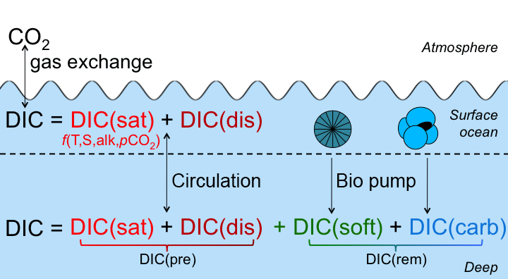
Figure 1 Illustration of the decomposition framework used for DIC in this paper. In the surface ocean, DIC is equal to DIC${}_{\mathrm{pre}}={\mathrm{DIC}}_{\mathrm{sat}}+{\mathrm{DIC}}_{\mathrm{dis}}$. Carbon taken up by biological processes in the surface ocean sinks and remineralizes in the water column to add two additional components at depths: DIC${}_{\mathrm{rem}}={\mathrm{DIC}}_{\mathrm{soft}}+{\mathrm{DIC}}_{\mathrm{carb}}$.

Saturation DIC is simply determined by the atmospheric CO₂ concentration and its solubility in seawater, which is a function of ocean temperature, salinity, and alkalinity. For example, cooling the ocean will increase CO₂ solubility, thereby leading to an increase in DIC_sat. Given known changes in temperature, salinity, alkalinity, and atmospheric pCO₂, the effective storage of DIC_sat can be calculated precisely.

At the ocean surface, primary producers take up DIC. The organic carbon that is formed then sinks or is subducted (as dissolved or suspended organic matter) and is transformed into remineralized DIC within the water column (a small fraction is buried at depth). Here we define DIC_soft as that which accumulates through the net respiration of organic matter below the top layer of the ocean (in our model, the uppermost 10 m). Thus, DIC_soft depends both on the export flux of organic matter, affected by surface ocean conditions including nutrient supply (Moore et al., 2013; Martin, 1990), and the ocean circulation as a whole, including the surface-to-deep export and the flushing rate of the deep ocean, which clears out accumulated DIC_soft (Toggweiler et al., 2003). The Southern Ocean (SO) is thought to be an important region for such changes on glacial/interglacial timescales, as the ecosystem there is currently iron-limited, and it also plays a major role in deep ocean ventilation (Martin, 1990; François et al., 1997; Toggweiler et al., 2003; Köhler and Fischer, 2006; Sigman et al., 2010; Watson et al., 2015; Jaccard et al., 2016). Assuming a constant global oceanic phosphate inventory and constant C : P ratio, DIC_soft is stoichiometrically related to the preformed ${\mathrm{PO}}_{\mathrm{4}}^{\mathrm{3}-}$ (${\mathrm{PO}}_{{\mathrm{4}}_{\mathrm{pre}}}^{\mathrm{3}-}$) inventory of the ocean, where ${\mathrm{PO}}_{{\mathrm{4}}_{\mathrm{pre}}}^{\mathrm{3}-}$ is the concentration of ${\mathrm{PO}}_{\mathrm{4}}^{\mathrm{3}-}$ in newly subducted waters, and a passively transported tracer in the interior. The potential to use ${\mathrm{PO}}_{{\mathrm{4}}_{\mathrm{pre}}}^{\mathrm{3}-}$ as a metric of DIC_soft prompted very fruitful efforts to understand how it could change over time (Ito and Follows, 2005; Marinov et al., 2008a; Goodwin et al., 2008), though it has been pointed out that the large variation in C : P of organic matter could weaken the relationship between DIC_soft and ${\mathrm{PO}}_{{\mathrm{4}}_{\mathrm{pre}}}^{\mathrm{3}-}$ (Galbraith and Martiny, 2015). Given that the variability of N : C is significantly smaller than P : C (Martiny et al., 2013), we use preformed nitrate in the discussion below.

Similar to DIC_soft, DIC_carb is defined here as the DIC generated by the dissolution of calcium carbonate shells below the ocean surface layer. Note that this does not include the impact that shell production has at the surface; calcification causes alkalinity to decrease in the surface ocean, raising surface pCO₂ and shifting carbon to the atmosphere. Rather, within the framework used here, this effect on alkalinity distribution falls under DIC_sat, since it alters the solubility of DIC. This highlights an important distinction between the four-component framework, which strictly defines subcomponents of DIC, and the “pump” frameworks, which provide looser descriptions of vertical fluxes of carbon and, in some cases, alkalinity. Changes in DIC_carb on the timescales of interest are generally thought to be small compared to those of DIC_sat and DIC_soft.

Typically, only these three components are considered as the conceptual drivers behind changes in the air–sea partitioning of pCO₂ (e.g., IPCC, 2007; Kohfeld and Ridgwell, 2009; Marinov et al., 2008a; Goodwin et al., 2008). However, a fourth component, DIC_dis, is also potentially significant as discussed by Ito and Follows (2013). Defined as the difference between preformed DIC and DIC_sat, DIC_dis can be relatively large (Takahashi et al., 2009) because of the slow timescale of atmosphere–surface ocean equilibrium of carbon compared to other gases, caused by the reaction of CO₂ with seawater (e.g., Zeebe and Wolf-Gladrow, 2001; Broecker and Peng, 1974; Galbraith et al., 2015). In short, DIC_dis is a function of all non-equilibrium processes on DIC in the surface ocean, including biological uptake, ocean circulation, and air–sea fluxes of heat, freshwater, and CO₂.

Like DIC_sat, DIC_dis is a conservative tracer determined in the surface ocean, with no sources or sinks in the ocean interior. Since the majority of the ocean is filled by water originating from small regions of the Southern Ocean and the North Atlantic, the net whole-ocean disequilibrium carbon is approximately determined by the DIC_dis in these areas weighted by the fraction of the ocean volume filled from each of these sites. Unlike the other three components, DIC_dis could contribute either additional oceanic carbon storage (DIC_dis > 0) or reduced oceanic carbon storage (DIC_dis<0). Although this parameter is implicitly included in most models, studies using preformed nutrients as a metric for biological carbon storage have often ignored the potential importance of DIC_dis by assuming fast air–sea gas exchange (e.g., Marinov et al., 2008a; Ito and Follows, 2005). In the pre-industrial ocean this is of little importance, given that global DIC_dis is small because the opposing effects of North Atlantic and Antarctic water masses largely cancel each other. However, Ito and Follows (2013) showed that DIC_dis can have a large impact by amplifying changes in DIC_soft under constant pre-industrial ocean circulation, and Ödalen et al. (2018) have very recently shown that DIC_dis can vary significantly in response to changes in ocean circulation states.

The cycling of dissolved oxygen is simpler than DIC. Because O₂ does not react with seawater or the dissolved constituents thereof, it has no dependence on alkalinity, and its equilibration with the atmosphere through air–sea exchange occurs approximately 1 order of magnitude faster than DIC (on the order of 1 month, rather than 1 year). Nonetheless, dissolved oxygen can be conceptualized as including a preformed component, which is the sum of saturation and disequilibrium, and an oxygen utilization component, which is given by the difference between the in situ and preformed O₂ in the ocean interior. Apparent oxygen utilization (AOU), typically taken as a measure of accumulated respiration, can be misleading if the preformed O₂ concentration differed significantly from saturation, i.e., if ${\mathrm{O}}_{{\mathrm{2}}_{\mathrm{dis}}}$ is significant, as it appears to be in high-latitude regions of dense water formation (Ito et al., 2004; Duteil et al., 2013; Russell and Dickson, 2003). If ${\mathrm{O}}_{{\mathrm{2}}_{\mathrm{dis}}}$ varies with climate state, it might contribute significantly to past or future oxygen concentrations.

Here, we use a complex Earth system model to investigate the potential changes in the constituents of DIC and O₂ on long timescales, relevant for past climate states as well as the future. We make use of a large number of equilibrium simulations, conducted over a wide range of radiative, orbital, and ice sheet boundary conditions, as a “library” of contrasting ocean circulations in order to test the response of disequilibrium carbon storage to physically plausible changes in ocean circulation. The basic physical aspects of these simulations were described by Galbraith and de Lavergne (2018). We supplement these with a smaller number of iron fertilization experiments to examine the additional impact of circulation-independent ecosystem changes. In order to simplify the interpretation, we chose to prescribe a constant pCO₂ of 270 ppm for the air–sea exchange in all simulations, as also done by Ödalen et al. (2018). Thus, the changes in DIC_sat reflect only changes in temperature, salinity, alkalinity, and ocean circulation arising from the climate response, and not changes in pCO₂. Nor do they explicitly consider changes in the total carbon or alkalinity inventories driven by changes in outgassing and/or burial (Roth et al., 2014; Tschumi et al., 2011); rather, the alkalinity inventory is fixed, and the carbon inventory varies due to changes in total ocean DIC (since the atmosphere is fixed). As such, the experiments here should be seen as idealized climate-driven changes, and should be further tested with more comprehensive models including interactive CO₂.

2 Methods

2.1 Model description

The global climate model (GCM) used in this study is CM2Mc, the Geophysical Fluid Dynamics Laboratory's Climate Model version 2 but at lower resolution (3^∘), described in more detail by Galbraith et al. (2011) and modified as described by Galbraith and de Lavergne (2018). This includes the Modular Ocean Model version 5, a sea ice module, static land, and static ice sheets, and a module of Biogeochemistry with Light, Iron, Nutrients and Gases (BLINGv1.5; Galbraith et al., 2010). Unlike BLINGv0, BLINGv1.5 allows for variable P : C stoichiometry using the “line of frugality” (Galbraith and Martiny, 2015) and calculates the mass balance of phytoplankton in order to prevent unrealistic bloom magnitudes at high latitudes, reducing the magnitude of disequilibrium O₂, which was very high in BLINGv0 (Duteil et al., 2013; Tagliabue et al., 2016). In addition, three water mass tracer tags are defined: a southern tracer south of 30^∘ S, a North Atlantic tracer north of 30^∘ N in the Atlantic, and a North Pacific tracer north of 30^∘ N in the Pacific. An “ideal age” tracer is also defined as zero in the global surface layer, and increasing in all other layers at a rate of 1 year per year.

2.2 Experimental design

The model runs analyzed here are part of the same suite of simulations discussed by Galbraith and de Lavergne (2018). A control run was conducted with a radiative forcing equivalent to 270 ppm atmospheric pCO₂ and the Earth's obliquity and precession set to modern values (23.4 and 102.9^∘, respectively). Experimental simulations were run at values of obliquity (22, 24.5^∘) and precession (90, 270^∘) representing the astronomical extremes encountered over the last 5 Myr (Laskar et al., 2004), while eccentricity was held constant at 0.03. A range of greenhouse radiative forcings was imposed equivalent to pCO₂ levels of 180, 220, 270, 405, 607, or 911 ppm; with reference to a pre-industrial radiative forcing, the radiative forcings are roughly equal to −2.2, −1.1, 0, +2.2, +4.3, and +6.5 W m⁻², respectively (Myhre et al., 1998).

The biogeochemical component of the model calculates air–sea carbon fluxes using a fixed atmospheric pCO₂ of 270 ppm throughout all model runs. Note that 270 ppm was chosen to reflect an average interglacial level, rather than specifically focusing on the pre-industrial climate state. This use of constant pCO₂ for the carbon cycle means that the DIC_sat is not consistent with the pCO₂ used for the radiative forcing, so that changes in DIC_sat caused by a given pCO₂ change tend to be larger than would be expected in reality. This has a negligible effect on the other carbon components, given that they do not depend directly on pCO₂; this has been confirmed by model runs with the University of Victoria Earth System Model using a similar decomposition strategy (Samar Khatiwala, personal communication, 2018).

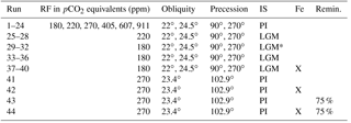
Eight additional runs were conducted using Last Glacial Maximum (LGM) ice sheets with the lowest two radiative forcings and the same orbital parameters. Iron fertilization simulations calculate the input flux of dissolved iron to the ocean surface assuming a constant solubility and using the glacial atmospheric dust field of Mahowald et al. (2006) as modified by Nickelsen and Oschlies (2015) instead of the standard pre-industrial dust field; note that this is not entirely in agreement with more modern reconstructions, which could potentially have an influence on the induced biological blooms, both in magnitude and geographically (e.g., Albani et al., 2012, 2016). Four iron fertilization experiments were run with the lowest radiative forcing with LGM ice sheets, as well as one model run similar to the control run. Finally, two simulations were run that were identical to the pre-industrial setup, but the rate of remineralization of sinking organic matter is set to 75 % of the default rate, approximately equivalent to the expected change due to 5 ^∘C ocean cooling (Matsumoto et al., 2007); one of these runs also includes iron fertilization. All simulations are summarized in Table 1.

Table 1 Simulation overview. A total of 44 simulations were analyzed with varying radiative forcing (RF), obliquity, precession, ice sheets (PI, pre-industrial; LGM, Last Glacial Maximum reconstruction; LGM*, topography of LGM ice sheets but with PI albedo), and with and without iron fertilization. Runs 1–40 are described by Galbraith and de Lavergne (2018). Runs 43 and 44 and identical to 41 and 42 but the remineralization rate of sinking organic matter is reduced by 25 %.

In the following, three particular runs are highlighted for comparison to illustrate cold (CW), moderate (MW), and hot (HW) worlds. These include radiative forcings of −2.2, 0, and +4.3 W m⁻², respectively; the former includes LGM ice sheets; and the obliquity and precession is 22 and 90^∘ for glacial-like (GL) and 22 and 270^∘ for PI and WP. These specific runs are distinguished from GL and interglacial-like (IG) scenarios, which refer to averages of four runs each, each with a radiative forcing of −2.2 and 0 W m⁻², respectively; the GL runs also have LGM ice sheets.

All simulations were run for 2100–6000 model years beginning with a pre-industrial spinup. While the model years presented here largely reflect runs after having reached steady state, it is important to note that the pre-industrial run (41 in Table 1) still has a drift of 1 µmol kg⁻¹ over the 100 years shown here and thus may not yet be at steady state.

2.3 Decompositions

The four-component DIC scheme and three-component O₂ scheme described in the introduction can be exactly calculated for any point in an ocean model using five easily implemented ocean model prognostic tracers: DIC, DIC_pre, DIC_sat, O₂, and O_2pre, since DIC${}_{\mathrm{dis}}={\mathrm{DIC}}_{\mathrm{pre}}-{\mathrm{DIC}}_{\mathrm{sat}}$, DIC${}_{\mathrm{soft}}=({\mathrm{O}}_{\mathrm{2}\mathrm{pre}}-{\mathrm{O}}_{\mathrm{2}})\cdot r_{\mathrm{C}:{\mathrm{O}}_{\mathrm{2}}}$, DIC${}_{\mathrm{carb}}=\mathrm{DIC}-{\mathrm{DIC}}_{\mathrm{pre}}-{\mathrm{DIC}}_{\mathrm{soft}}$, and O_2dis = O_2pre − O_2sat (O_2sat can be accurately calculated from the conservative tracers temperature and salinity). In the absence of a DIC_sat tracer, it can be estimated from alk_pre, temperature, and salinity. For this large suite of simulations, we only had DIC, alk, O₂, and O_2pre available. Thus, although we could calculate O_2dis and DIC_soft directly, it was necessary to use an indirect method to calculate the other three carbon tracers. Following Bernardello et al. (2014), we first estimate alk_pre using a regression, then calculate DIC_sat using alk_pre, temperature, salinity, and the known atmospheric pCO₂ of 270 ppm. DIC_carb is calculated as $\mathrm{0.5}\cdot (\mathrm{alk}-{\mathrm{alk}}_{\mathrm{pre}})$, and DIC_dis is then calculated as a residual. For more details and an estimate of the error in the method, see the Appendix.

3 Results and discussion

3.1 General climate response to forcings

Differences in the general ocean state among the model simulations are described in detail by Galbraith and de Lavergne (2018). We provide here a few key points, important for interpreting the dissolved gas simulations. First, the Antarctic Bottom Water (AABW) fraction of the global ocean varies over a wide range among the simulations, with abundant AABW under low and high global average surface air temperature (SAT), and a minimum at intermediate SAT (Fig. 2b). The North Atlantic deep water (NADW) fraction is approximately the inverse of this. The ventilation rate of the global ocean is roughly correlated with the AABW fraction, with rapid ventilation (small average ideal age) when the AABW fraction is high (Fig. 2). The density difference between AABW and NADW is the overall driver of the AABW fraction and ventilation rate in the model simulations. In all simulations colder than the present day, the density difference can be explained by the effect of sea ice cycling in the Southern Ocean on the global distribution of salt: when the Southern Ocean is cold and sea ice formation abundant, there is a large net transport of freshwater out of the circum-Antarctic, causing AABW to become more dense. NADW becomes consequently fresher, because there is less salt left to contribute to NADW. As noted by Galbraith and de Lavergne (2018), the simulated ventilation rates should be viewed with caution, given the poor mechanistic representation of diapycnal mixing in the deep ocean, and the AABW fraction may not be correlated with ventilation rate in the real ocean.

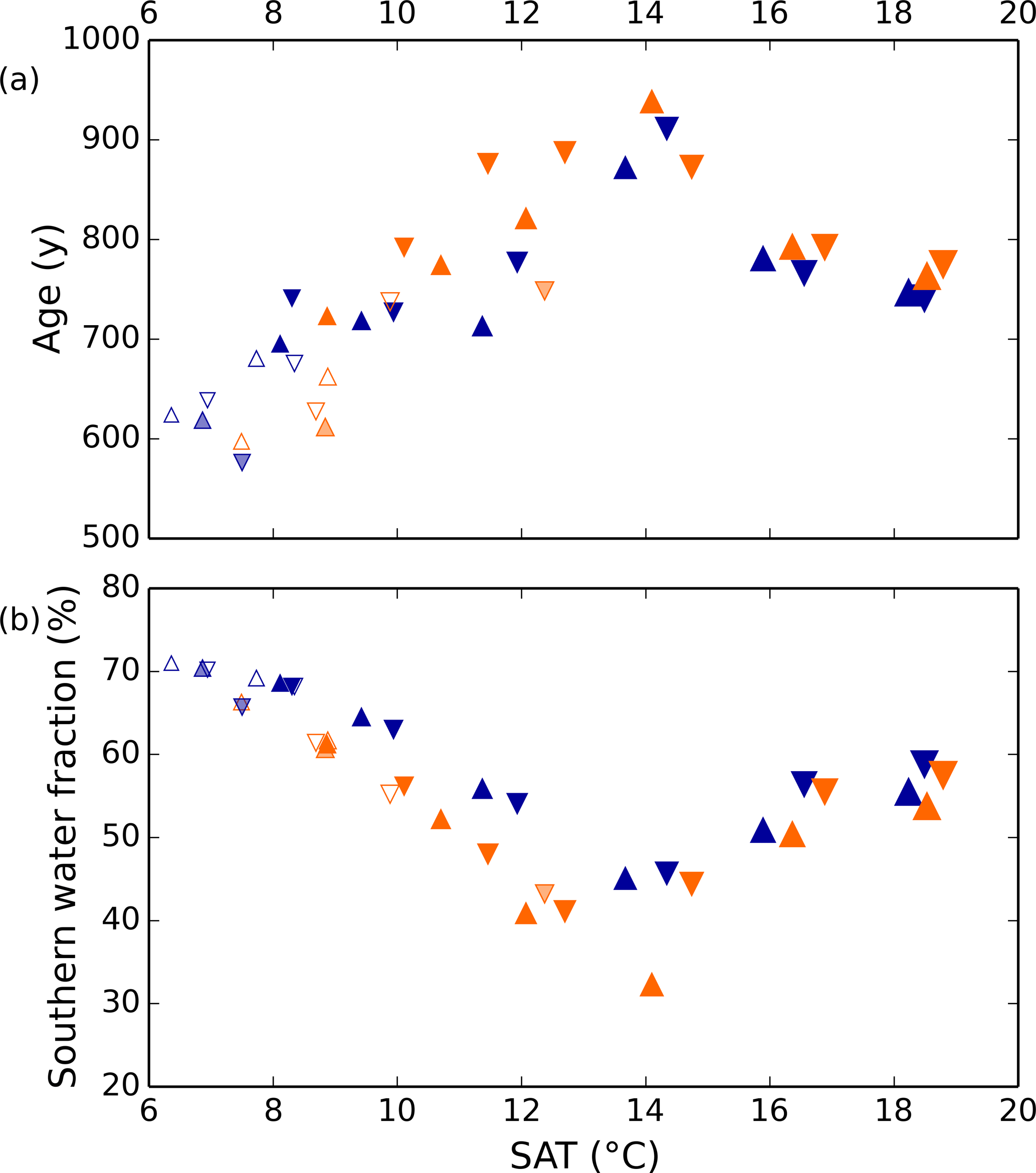
Figure 2 Simulated global ocean ventilation and proportion of southern-sourced deepwater. The horizontal axis shows the globally averaged surface air temperature (SAT). (a) The global ocean average ideal age (low age corresponds to rapid ventilation) and (b) the fraction of water in the global ocean originating from the surface south of 30^∘ S are anti-correlated over the range of SAT in these model runs. Orange and blue symbols represent high and low obliquity scenarios, respectively; triangles pointing upward and downward represent greater Northern and Southern hemisphere seasonality (precession 270 and 90^∘); outlines are scenarios with LGM ice sheets; light shading indicates scenarios with LGM ice sheet topography but PI albedo. The size of the symbols corresponds to the SAT.

3.2 General changes in DIC

Total DIC generally decreases from cold to warm simulations, under the constant pCO₂ of 270 ppm used for air–sea exchange. Changes in DIC_sat drive the largest portion of this trend, decreasing approximately linearly with surface air temperature due to the temperature-dependence of CO₂ solubility, resulting in a difference of 50 µmol kg⁻¹ over this range (see Fig. 3). Because of the constant pCO₂ of 270 ppmv in the biogeochemical module, the simulated range of DIC_sat is larger than would occur if the prescribed biogeochemical pCO₂ were the same as that used to produce the low SAT (Ödalen et al., 2018). DIC_carb is relatively small in magnitude and generally increases with SAT, but has a standard deviation of only 4 µmol kg⁻¹ over all simulations, so we do not discuss it further.

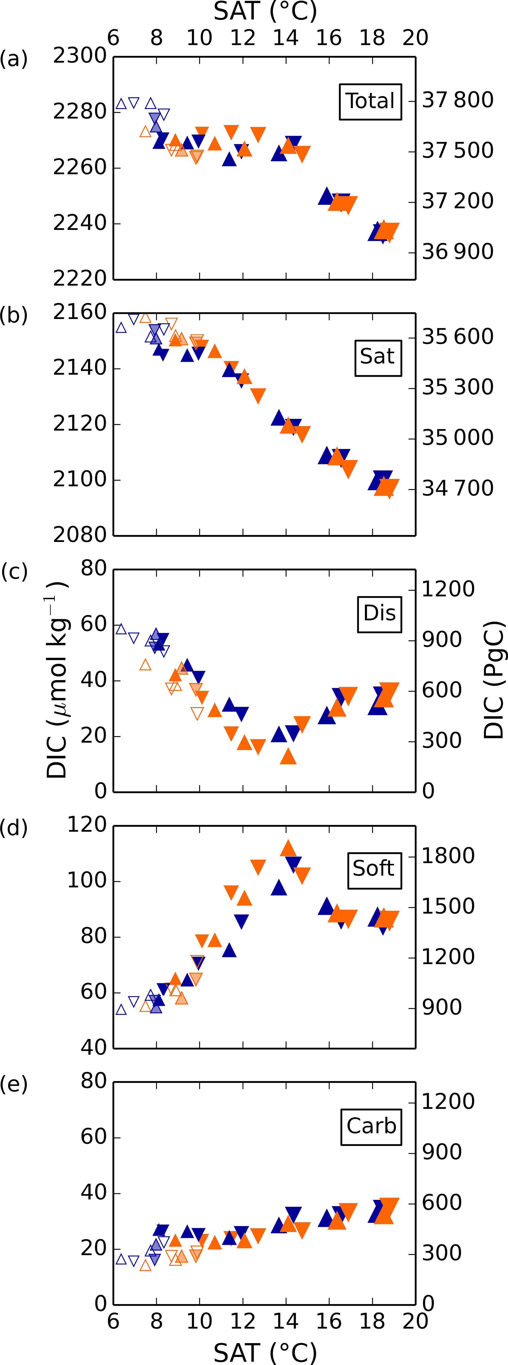
Figure 3 Global average DIC and separate components in simulations 1–36 as a function of globally averaged surface air temperature (SAT). Orange and blue symbols represent high and low obliquity scenarios, respectively; triangles pointing upward and downward represent greater Northern and Southern hemisphere seasonality (precession 270 and 90^∘); outlines are scenarios with LGM ice sheets; light shading indicates scenarios with LGM ice sheet topography but PI albedo.

In contrast to DIC_sat and DIC_carb, DIC_dis and DIC_soft vary nonlinearly with global temperatures, with a clear and shared turning point near the middle of the temperature range. Thus, the extreme values of DIC_soft and DIC_dis occur under the coldest state and at an intermediate state close to the pre-industrial. Both DIC_dis and DIC_soft are strongly correlated with ocean ventilation, quantified here by the global average of the ideal age tracer (r²=0.69 and 0.89, respectively), and thus with each other (r²=0.74). However, whereas Ito and Follows (2013) found a positive correlation of DIC_soft and DIC_dis under nutrient depletion experiments with constant climate, these experiments indicate that, when driven by the wide range of physical changes explored here, DIC_soft and DIC_dis are negatively correlated.

Simulated changes in DIC_dis are of the same magnitude as the DIC_soft changes, to which much greater attention has been paid. For a global average buffer factor between 8 and 14 (Zeebe and Wolf-Gladrow, 2001), a rough, back-of-the-envelope calculation shows that a 1 µmol kg⁻¹ change in DIC corresponds to a 0.9–1.6 ppm change in atmospheric pCO₂ based on a DIC concentration of 2300 µmol kg⁻¹ and pCO₂ of 270 ppm. Thus, the increase in the global average DIC_dis in these simulations could have contributed more than a 40 ppm change in the atmospheric pCO₂ stored in the ocean during the glacial compared to today. It is important to recognize that the drawdown of CO₂ by disequilibrium storage would have resulted in a decrease of DIC_sat, given the dependence of the saturation concentration on pCO₂, so this estimate should not be interpreted as a straightforward atmospheric pCO₂ change. Nonetheless, while this is only a first-order approximation and the model biases are potentially large, it seems very likely that the disequilibrium carbon storage was a significant portion of the net 90 ppm difference.

3.3 Climate-driven changes in DIC_soft

The biogeochemical model used here is relatively complex, with limitation by three nutrients (N, P, and Fe), denitrification, and N₂ fixation, in addition to the temperature- and light-dependence typical of biogeochemical models. The climate model is also complex, including a full atmospheric model, a highly resolved dynamic ocean mixed layer, and many nonlinear sub-grid-scale parameterizations, and uses short (< 3 h) timesteps. The simulations we show span a wide range of behaviors, including major changes in ocean ventilation pathways and patterns of organic matter export.

Thus, it is perhaps surprising that the net global result of the biological pump, as quantified by DIC_soft, has highly predictable behavior. As shown in Fig. 4, the global DIC_soft varies closely with the product of the global average sinking flux of organic matter at 100 m and the average ideal age of the global ocean. Qualitatively this is not a surprise, given that greater export pumps more organic matter to depth, and a large age provides more time for respired carbon to accumulate within the ocean. However, the quantitative strength of the relationship is striking. As demonstrated in Fig. 4, global DIC_soft is not as well correlated with either of these parameters separately as it is with their product “age × export”.

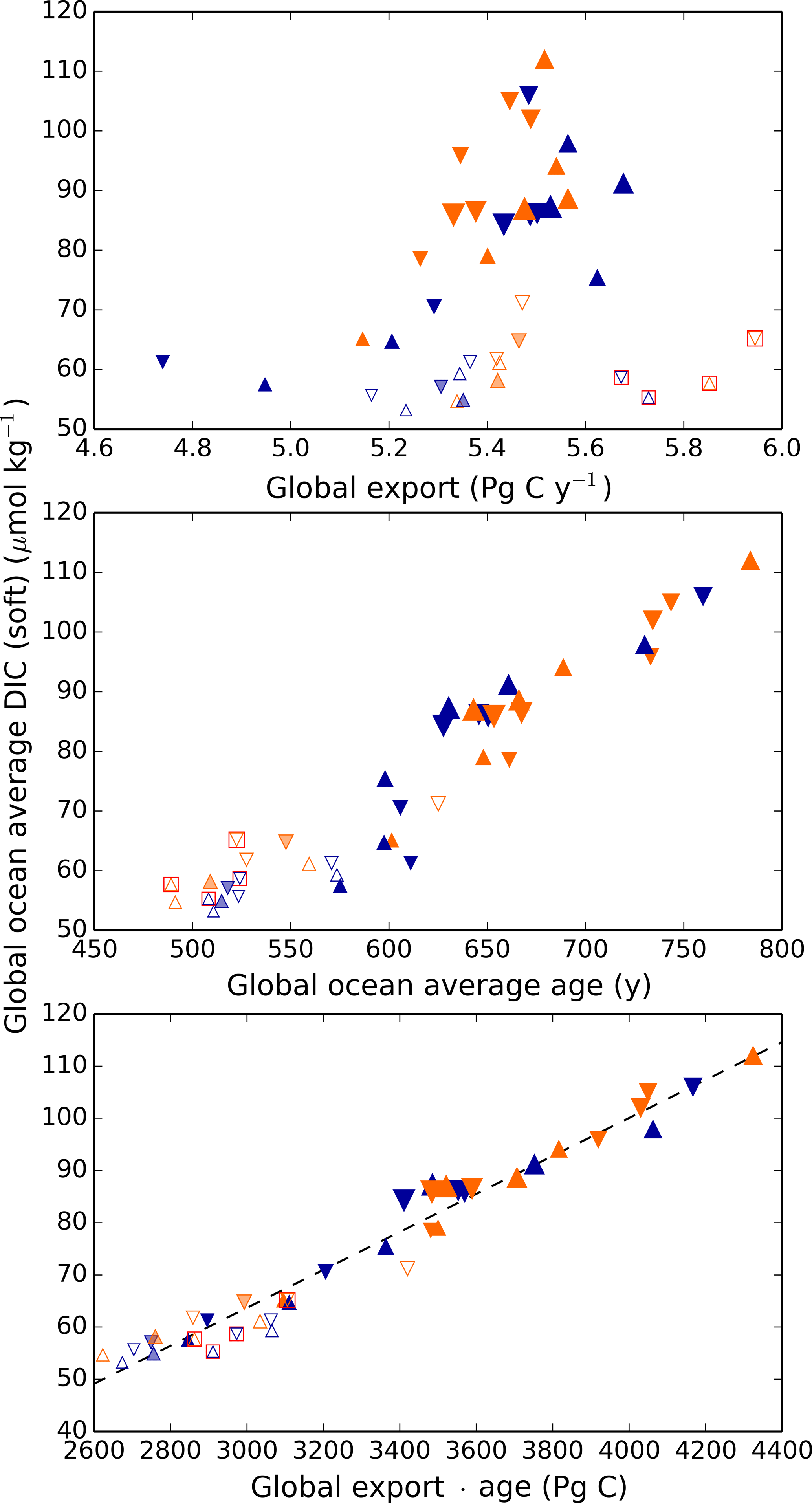
Figure 4 Globally averaged DIC_soft vs. global export, ideal age, and age × export. Globally averaged DIC_soft can be approximated remarkably well by the global export flux of organic carbon at 100 m multiplied by the average age of the ocean. The latter is an ideal age tracer in the model that is set to 0 at the surface and ages by 1 year each model year in the ocean interior. Orange and blue symbols represent high and low obliquity scenarios, respectively; triangles pointing upward and downward represent greater Northern and Southern hemisphere seasonality (precession 270 and 90^∘); outlines are scenarios with LGM ice sheets; light shading indicates scenarios with LGM ice sheet topography but PI albedo. Red boxes indicate Fe fertilization simulations (runs 37–40). The size of the symbols corresponds to the SAT.

It is difficult to assess the likelihood that the real ocean follows this relationship to a similar degree. One reason it might differ is if remineralization rates vary spatially, or with climate state. In the model here, as in most biogeochemical models, organic matter is respired according to a globally uniform power law relationship with depth (Martin et al., 1987). Kwon et al. (2009) showed that ocean carbon storage is sensitive to changes in these remineralization rates, which provides an additional degree of freedom. It is not currently known how much remineralization rates can vary naturally; they may vary as a function of temperature (Matsumoto et al., 2007) or ecosystem structure. As a result, the relationship between DIC_soft and age × export may be stronger in the model than in the real ocean.

Nonetheless, the results suggest that, as a useful first-order approximation, the global change in DIC_soft between two states can be given by a simple linear regression:

$$\begin{array}{}\text{(1)}& {\displaystyle }\mathrm{\Delta }{\mathrm{DIC}}_{\mathrm{soft}}\left[\mathrm{\mu }\mathrm{mol}{\mathrm{kg}}^{-\mathrm{1}}\right]=m_{\mathrm{1}}\cdot \mathrm{\Delta }\left(\mathrm{age}\right[\mathrm{yr}]\times \mathrm{export}[\mathrm{Pg}\mathrm{C}{\mathrm{yr}}^{-\mathrm{1}}\left]\right),\end{array}$$

or in terms of pCO₂:

$$\begin{array}{}\text{(2)}& {\displaystyle }\mathrm{\Delta }p{\mathrm{CO}}_{\mathrm{2},\mathrm{soft}}\left[\mathrm{ppm}\right]\approx m_{\mathrm{2}}\cdot \mathrm{\Delta }\left(\mathrm{age}\right[\mathrm{yr}]\times \mathrm{export}[\mathrm{Pg}\mathrm{C}{\mathrm{yr}}^{-\mathrm{1}}\left]\right).\end{array}$$

Note that m₂ is a function of the buffer factor and the climate state (atmospheric pCO₂ and DIC). Based on the results here, m₁=0.036 and $m_{\mathrm{2}}=\mathrm{0.065},\mathrm{0.042},\mathrm{0.029}$ for modern (405 ppm pCO₂), pre-industrial (270 ppm) and glacial (180 ppm) conditions, respectively. Note that we have not varied pCO₂ in these simulations, so these equations are only meant to illustrate the mathematical relationship observed in Fig. 4. This simple meta-model may provide a useful substitute for full ocean–ecosystem calculations, and should be further tested against other ocean–ecosystem coupled models with interactive CO₂. Note that, as for the disequilibrium estimate above, the soft tissue pump CO₂ drawdown is partially compensated for by a decrease in saturation carbon storage, so it would be larger than the net atmospheric effect. In addition, we have not accounted for consequent changes in the surface ocean carbonate chemistry (including changes in the buffer factor).

It is important to point out that the simulated change in DIC_soft between interglacial and glacial states appears to be in conflict with reconstructions of the LGM. Proxy records appear to show that LGM dissolved oxygen concentrations were lower throughout the global ocean, with the exception of the North Pacific, implying greater DIC_soft concentrations during the glacial then during the Holocene (Galbraith and Jaccard, 2015). In contrast, the model suggests that greater ocean ventilation rates in the glacial state (Fig. 2a) would have led to reduced global DIC_soft. As discussed by Galbraith and de Lavergne (2018), radiocarbon observations imply that the model ideal age is approximately 200 years too young under glacial conditions compared to the LGM, suggesting a circulation bias that may reflect incorrect diapycnal mixing or non-steady-state conditions. Whatever the cause, if we take this 200-year bias into account, the regression implies that an additional 33 µmol kg⁻¹ DIC_soft were stored in the glacial ocean. This would bring the simulated glacial DIC_soft close to, but still less than, the simulated pre-industrial value.

We propose that the apparent remaining shortfall in simulated glacial DIC_soft could reflect one or more of the following non-exclusive possibilities: (1) the model does not capture changes in remineralization rates caused by ecosystem changes; (2) the model underestimates the glacial increase in the nitrate inventory and/or growth rates, perhaps due to changes in the iron cycle; (3) the ocean was not in steady state during the LGM, and therefore not directly comparable to the GL simulation; (4) the inference of DIC_soft from proxy oxygen records is incorrect due to significant changes in preformed oxygen disequilibrium (see below). If either of the first two possibilities is important, it would imply an inaccuracy in the meta-model derived here.

3.4 Climate-driven changes in DIC_dis

The ocean basins below 1 km depth are largely filled by surface waters subducted to depth in regions of deepwater formation (Gebbie and Huybers, 2011). In our simulations, water originating in the surface North Atlantic, termed NADW, and the Southern Ocean, termed AABW, make up 80–96 % of this total deep ocean volume. Thus, to first order, the deep average DIC_dis concentration can be approximated by a simple mass balance:

$$\begin{array}{ll}{\displaystyle }{\mathrm{DIC}}_{{\mathrm{dis}}_{\mathrm{deep}}}\approx & {\displaystyle }{f}_{\mathrm{AABW}}\cdot {\mathrm{DIC}}_{{\mathrm{dis}}_{\mathrm{AABW}}}+(\mathrm{1}-f_{\mathrm{AABW}})\\ \text{(3)}& {\displaystyle }& {\displaystyle }\cdot {\mathrm{DIC}}_{{\mathrm{dis}}_{\mathrm{NADW}}}.\end{array}$$

Here, f_AABW represents the fraction of deepwater originating in the SO, and DIC${}_{{\mathrm{dis}}_{\mathrm{AABW}}}$ and DIC${}_{{\mathrm{dis}}_{\mathrm{NADW}}}$ represent the DIC_dis concentrations at the sites of deepwater formation (see Fig. 5). North Atlantic deep water forms with negative DIC_dis, reflecting surface undersaturation, while the Southern Ocean is supersaturated (DIC_dis>0). These opposing tendencies between NADW and AABW cause a partial cancellation of DIC_dis when globally averaged, which makes the disequilibrium component small in the modern ocean. Theoretically, the simulated DIC_dis could change either due to changes in f_AABW or the end-member compositions. Although the exact values of DIC_dis in the two polar oceans vary among the simulations in response to climate (the reasons for which are discussed in more detail below), these changes are small relative to the consistent large contrast between f_AABW and f_NADW, so that deep DIC_dis is strongly controlled by the global balance of AABW vs. NADW in each simulation (see Fig. 6). Global DIC_dis becomes much larger when f_AABW is larger, similar to the dynamic evoked by Skinner (2009). This is also illustrated by the depth transects of DIC_dis in Fig. 7.

Figure 5 (a) Global average fraction of northern- (reddish colors) and southern-sourced (bluish colors) water. (b) Annual average values of DIC_dis of these water masses determined at 25 m depth in the model during model years and at locations where deep convection occurs. Pink and cyan (red and blue) symbols represent high (low) obliquity scenarios; triangles pointing upward and downward represent greater Northern and Southern hemisphere seasonality (precession 270 and 90^∘); outlines are scenarios with LGM ice sheets; light shading indicates scenarios with LGM ice sheet topography but PI albedo. Five simulations, for which no deep convection events were identified south of 60^∘S, are not shown. The size of the symbols corresponds to the SAT.

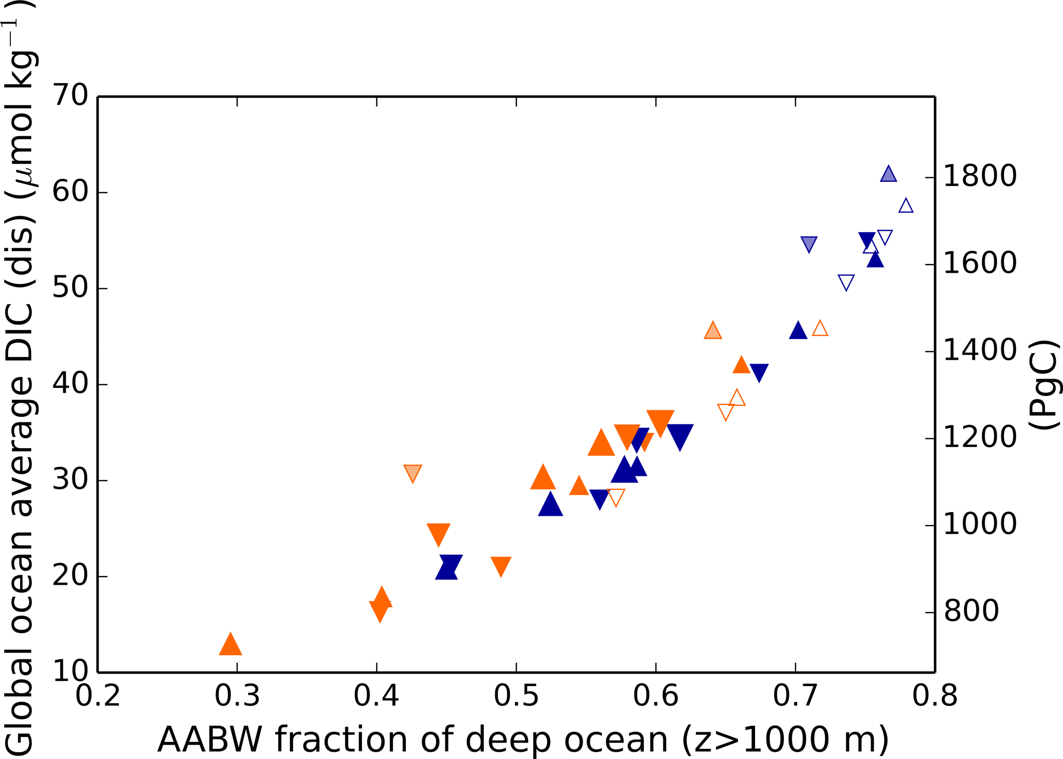
Figure 6 Global average DIC_dis as a function of the fraction of the ocean below 1 km derived from the surface Southern Ocean. Orange and blue symbols represent high and low obliquity scenarios, respectively; triangles pointing upward and downward represent greater Northern and Southern hemisphere seasonality (precession 270 and 90^∘); outlines are scenarios with LGM ice sheets; light shading indicates scenarios with LGM ice sheet topography but PI albedo. The size of the symbols corresponds to the SAT.

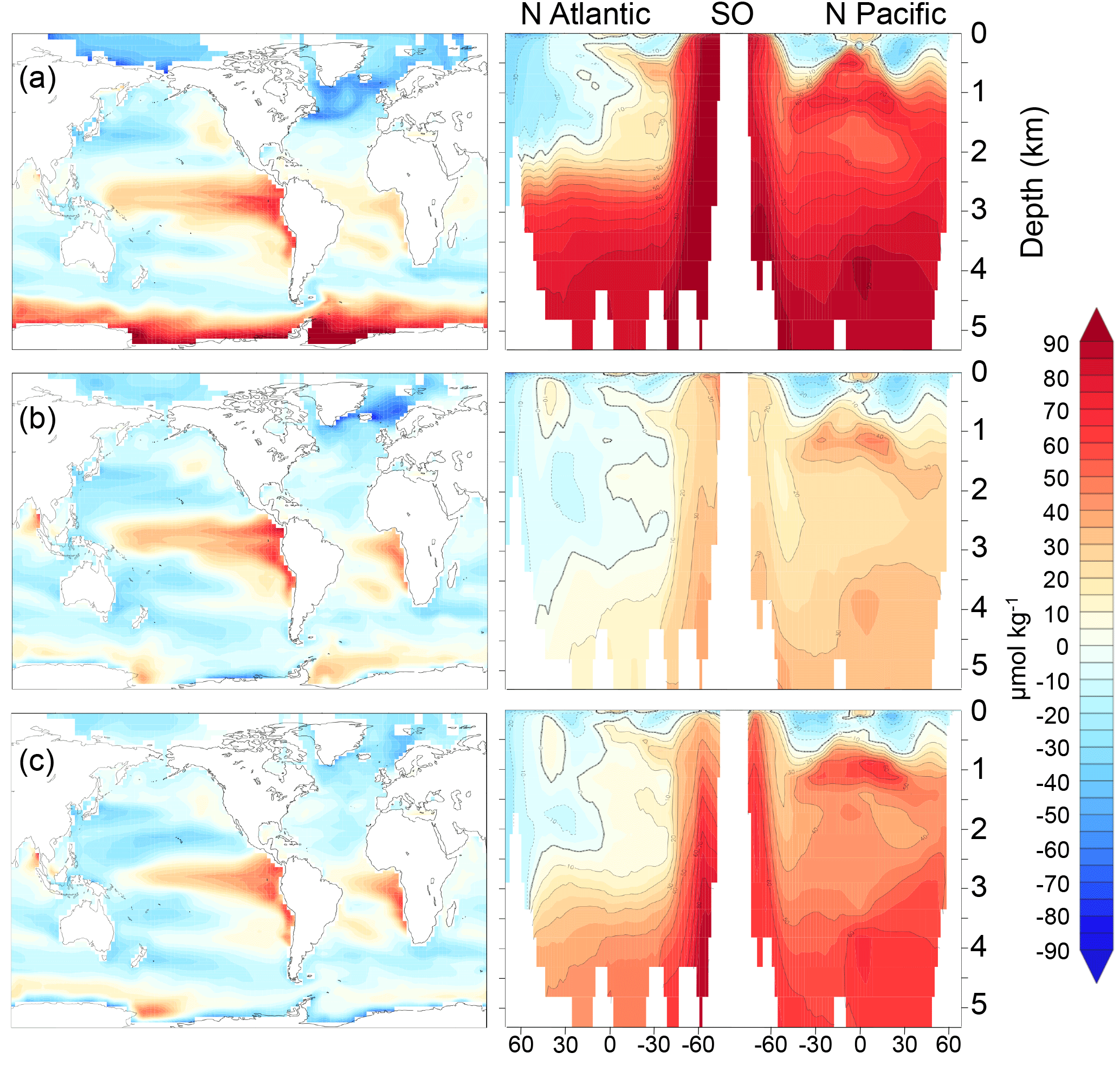
Figure 7 DIC_dis (µmol kg⁻¹) for simulations (a) cold world; (b) moderate world; (c) hot world (see Sect. 2.2). Depth transects represent the North Atlantic (left), Southern Ocean (center), and North Pacific (right).

We estimated the concentration of DIC_dis in the regions of AABW and NADW formation, shown in Fig. 5b. The end members vary less significantly than f_AABW over the range of simulations, in part due to competing effects of different processes. As discussed in Sect. 3.1, simulations at both the low and high radiative forcing values used show increased AABW production, with a minimum at intermediate values (Fig. 5). The fact that the highest DIC${}_{{\mathrm{dis}}_{\mathrm{AABW}}}$ occurs at low SAT can be attributed to the rapid formation rate of AABW, while the intermediate SAT minimum in AABW volume explains the minimum in global ocean DIC_dis (Fig. 3). We note that expanded terrestrial ice sheets shift the ratio of AABW to NADW to higher values, due to their impact on NADW temperature and downstream expansion of Southern Ocean sea ice (Galbraith and de Lavergne, 2018), further increasing DIC_dis in glacial-like conditions. Sea ice in the Southern Ocean would be expected to exert a further control over DIC_dis, as this reduces air–sea gas exchange, thus allowing carbon to accumulate beneath the ice. However we did not perform experiments to isolate this effect.

3.5 Climate-driven changes in ${\mathrm{O}}_{{\mathrm{2}}_{\mathrm{dis}}}$

Similarly to DIC_dis, ${\mathrm{O}}_{{\mathrm{2}}_{\mathrm{dis}}}$ is defined as the departure from equilibrium of O₂ in the surface ocean with respect to the atmosphere and is advected into the ocean as a conservative tracer. Unlike C, O₂ does not react with seawater, and is present only as dissolved diatomic oxygen. Thus, O₂ has a much shorter timescale of exchange at the ocean–atmosphere interface, equilibrating 1 order of magnitude faster than CO₂. As a result, it is not sensitive to sea ice as long as there remains a fair degree of open water (Stephens and Keeling, 2000). But as the sea ice concentration approaches complete coverage, O₂ equilibration rapidly becomes quite sensitive to sea ice. If there is a significant undersaturation of O₂ in upwelling waters, the disequilibrium can become quite large (Fig. 8).

Figure 8 ${\mathrm{O}}_{{\mathrm{2}}_{\mathrm{dis}}}$ (µmol kg⁻¹) for simulations (a) cold world; (b) moderate world; (c) hot world (see Sect. 2.2). Depth transects represent the North Atlantic (left), Southern Ocean (center), and North Pacific (right).

In the model simulations, the ${\mathrm{O}}_{{\mathrm{2}}_{\mathrm{dis}}}$ in the Southern Ocean becomes as large as −100 µmol kg⁻¹ in the coldest states (note that DIC_dis and ${\mathrm{O}}_{{\mathrm{2}}_{\mathrm{dis}}}$ are often anti-correlated). Because the disequilibrium depends on the O₂ depletion of waters upwelling at the Southern Ocean surface, this could potentially be even larger if upwelling waters had lower O₂. We do not place a large degree of confidence in these values, given the likely sensitivity to poorly resolved details of sea ice dynamics (e.g., ridging, leads) and dense water formation. Nonetheless, the potential for very large disequilibrium oxygen under cold states prompts the hypothesis that very extensive sea ice cover over most of the exposure pathway in the Southern Ocean might have made a significant contribution to the low O₂ concentrations reconstructed for the glacial (Jaccard et al., 2016; Lu et al., 2015).

3.6 Iron fertilization experiments

In addition to the changes driven by ice sheets as well as orbital and radiative forcing, we conducted iron fertilization experiments under glacial and pre-industrial-like conditions, including a simulation with reduced remineralization rates (Fig. 9). As expected, both the global export and DIC_soft increase when iron deposition is increased. However, the DIC_soft increase is significantly lower in the well-ventilated GL simulations (2.9 µmol kg⁻¹) compared to the PI simulation (7.3 µmol kg⁻¹). This difference is qualitatively in accordance with the age × export relationship (Fig. 4), though with a smaller increase of DIC_soft than would be expected from the export increase, compared to the broad spectrum of climate-driven changes. This reduced sensitivity of DIC_soft to the global export can be attributed to the fact that the iron-enhanced export occurs in the Southern Ocean, presumably because the remineralized carbon can be quickly returned to the surface by upwelling when ventilation is strong. Thus, the impact of iron fertilization on DIC_soft is strongly dependent on Southern Ocean circulation.

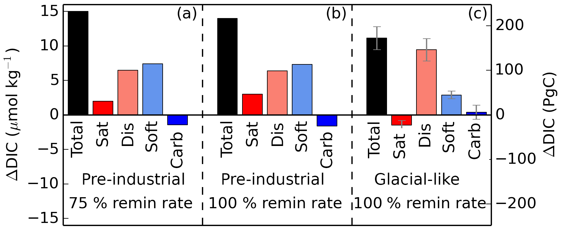
Figure 9 Iron-fertilized changes in total global average DIC and each of the components (iron fertilization simulation minus associated control run). Simulations were either run under pre-industrial or glacial-like conditions (in the case of the latter, results represent the average of the four GL runs, with error bars showing the standard deviation within the four runs), as well as using 100 and 75 % of the default remineralization rate of organic matter. The close agreement of panels (a) and (b) indicates that the effects of iron fertilization and changes in the remineralization rate are approximately linearly additive in this model.

The iron addition also causes an increase of DIC_dis of approximately equal magnitude to DIC_soft in the PI simulation and of relatively greater proportion in the GL simulations. Because the ocean in the GL simulations is strongly ventilated, the increase in export leads to an increase of DIC_dis, as remineralized DIC_soft is returned to the Southern Ocean surface, where it has a relatively short residence time that limits outgassing to the atmosphere. With rapid Southern Ocean circulation, a good deal of the DIC sequestered by iron fertilization ends up in the form of DIC_dis, rather than DIC_soft as might be assumed. Thus, just as the glacial state has a larger general proportion of DIC_dis compared to DIC_soft, the iron addition under the glacial state produces a larger fraction of DIC_dis relative to DIC_soft. The experiment in which the remineralization rate was reduced by 25 % indicates that the effects of iron fertilization alone on both DIC_soft and DIC_dis are quite insensitive to the remineralization rate (see Fig. 9); for total DIC as well as for each component, the difference between the iron fertilization run and the corresponding control run is similar in panels (a) and (b). While we have not run a simulation under glacial-like conditions with a reduced remineralization rate, this suggests that the effects of iron fertilization and changes in the remineralization rate can be well approximated as being linearly additive in this model.

The tendency to sequester carbon as DIC_dis vs. DIC_soft, in response to iron addition, can be quantified by the global ratio ΔDIC_dis ∕ ΔDIC_soft. Our experiments suggest that this ratio is 0.9 for the pre-industrial state and 3.3 for the glacial-like state. Because of the circulation dependence of this ratio, it is expected that there could be significant variation between models. It is worth noting that Parekh et al. (2006) found ΔDIC_dis ∕ ΔDIC_soft of 2 in response to iron fertilization, using a modern ocean circulation, as analyzed by Ito and Follows (2013). We also note that the quantitative values of DIC_soft and DIC_dis resulting from the altered iron flux should be taken with a grain of salt, given the very large uncertainty in iron cycling models (Tagliabue et al., 2016).

These results provide a note of caution for interpreting iron fertilization model experiments, which might be assumed to act primarily on the soft tissue carbon storage. At moderate ventilation rates (the pre-industrial control run), an increase in iron results in an increase both in DIC_soft, due to higher biological export, and DIC_dis, because of the upwelling of C-rich water resulting from higher remineralization, the effect discussed by Ito and Follows (2013). However, under a high ventilation state there is only a small increase in DIC_soft in response to increased Fe in the surface ocean, as the remineralized carbon is quickly returned to the surface, thus producing a significant increase in DIC_dis only. Thus, the carbon storage resulting from Southern Ocean iron addition could actually be dominated by DIC_dis under some climate states, so that the overall impact may be significantly larger than would be predicted from DIC_soft and/or O₂ utilization.

3.7 A unified framework for DIC_dis and preformed nutrients

The concept of preformed nutrients allowed the production of a very useful body of work, striving for simple predictive principles. This work highlighted the importance of the nutrient concentrations in polar oceans where deep waters form (Sigman and Boyle, 2000; Ito and Follows, 2005; Marinov et al., 2008a) as well as changes in the ventilation fractions of AABW and NADW, given their very different preformed nutrient concentrations (Schmittner and Galbraith, 2008; Marinov et al., 2008b). Although the variability of P : C ratios implies significant uncertainty for the utility of ${\mathrm{PO}}_{{\mathrm{4}}_{\mathrm{pre}}}^{\mathrm{3}-}$ in the ocean, the relative constancy of N : C ratios suggests that ${\mathrm{NO}}_{{\mathrm{3}}_{\mathrm{pre}}}^{-}$ is indeed linked to DIC_soft, inasmuch as the global N inventory is fixed (Galbraith and Martiny, 2015).

Figure 10 Simple estimation of global DIC_dis and DIC_soft from water mass characteristics. Following Eq. (12) for (a) DIC_soft and (b) DIC_dis separately, this model shows that the sum of the global average DIC_soft and DIC_dis at steady state can be estimated fairly robustly as the result of a simple mass balance of the relevant parameters in the most important ventilating water masses. Here, we take into account upper-ocean water masses (above 1 km) formed in the North Pacific, North Atlantic, and Southern Ocean, and deep water masses formed in the North Atlantic and Southern Ocean. In each plot, the full model output is shown on the x axis and the result of the mass balance approximation on the y axis. Orange and blue symbols represent high and low obliquity scenarios, respectively; triangles pointing upward and downward represent greater Northern and Southern hemisphere seasonality (precession 270 and 90^∘); outlines are scenarios with LGM ice sheets; light shading indicates scenarios with LGM ice sheet topography but PI albedo. Five simulations, for which no deep convection events were identified south of 60^∘S, are not shown. The size of the symbols corresponds to the SAT. The purple square represents the pre-industrial simulation (run 41), and red boxes indicate Fe fertilization simulations (runs 37–40).

However, as shown by the analyses here, DIC_soft – reflected by the preformed nutrients – is only half the story. Changes in DIC_dis can be of equivalent magnitude, and can vary independently of DIC_soft as a result of changes in ocean circulation and sea ice. Nonetheless, we find that the same conceptual approach developed for DIC_soft can be used to predict DIC_dis from the end member DIC_dis and the global volume fractions. The preformed relationships and DIC_dis can therefore be unified as follows (see Fig. 10):

$$\begin{array}{}\text{(4)}& {\displaystyle }{\mathrm{DIC}}_{\mathrm{soft}}={\mathrm{NO}}_{{\mathrm{3}}_{\mathrm{rem}}}^{-}\cdot r_{\mathrm{C}:\mathrm{N}}.\end{array}$$

Remineralized nitrate can be expressed in terms of the global nitrate inventory and the accumulated nitrate loss due to pelagic and benthic denitrification:

$$\begin{array}{ll}\text{(5)}& {\displaystyle }& {\displaystyle }{\mathrm{NO}}_{{\mathrm{3}}_{\mathrm{rem}}}^{-}={\mathrm{NO}}_{{\mathrm{3}}_{\mathrm{global}}}^{-}-{\mathrm{NO}}_{{\mathrm{3}}_{\mathrm{pre}}}^{-}+{\mathrm{NO}}_{{\mathrm{3}}_{\mathrm{den}}}^{-},{\displaystyle }& {\displaystyle }{\mathrm{NO}}_{{\mathrm{3}}_{{\mathrm{pre}}_{\mathrm{upper}}}}^{-}\approx f_{\mathrm{SO},\mathrm{upper}}\cdot {\mathrm{NO}}_{{\mathrm{3}}_{{\mathrm{pre}}_{\mathrm{SO},\mathrm{upper}}}}^{-}+f_{\mathrm{NAtl},\mathrm{upper}}\\ \text{(6)}& {\displaystyle }& {\displaystyle }\cdot {\mathrm{NO}}_{{\mathrm{3}}_{{\mathrm{pre}}_{\mathrm{NAtl},\mathrm{upper}}}}^{-}+f_{\mathrm{NPac},\mathrm{upper}}\cdot {\mathrm{NO}}_{{\mathrm{3}}_{{\mathrm{pre}}_{\mathrm{NPac},\mathrm{upper}}}}^{-},\text{(7)}& {\displaystyle }& {\displaystyle }{\mathrm{NO}}_{{\mathrm{3}}_{{\mathrm{pre}}_{\mathrm{deep}}}}^{-}\approx f_{\mathrm{AABW}}\cdot {\mathrm{NO}}_{{\mathrm{3}}_{{\mathrm{pre}}_{\mathrm{AABW}}}}^{-}+f_{\mathrm{NADW}}\cdot {\mathrm{NO}}_{{\mathrm{3}}_{{\mathrm{pre}}_{\mathrm{NADW}}}}^{-}.\end{array}$$

Because there is production of intermediate water but no deep convection in the North Pacific, we calculate this mass balance for the upper ocean (above 1 km) and deep ocean separately, dropping the Pacific Ocean term in Eq. (7) for the deep ocean. For brevity, we continue with the derivation for the deep ocean only; the upper ocean follows analogously.

$$\begin{array}{ll}{\displaystyle }& {\displaystyle }{\mathrm{DIC}}_{{\mathrm{soft}}_{\mathrm{deep}}}\approx r_{\mathrm{C}:\mathrm{N}}\cdot [{\mathrm{NO}}_{{\mathrm{3}}_{\mathrm{deep}}}^{-}+{\mathrm{NO}}_{{\mathrm{3}}_{\mathrm{den},\mathrm{deep}}}^{-}\\ \text{(8)}& {\displaystyle }& {\displaystyle }-(f_{\mathrm{AABW}}\cdot {\mathrm{NO}}_{{\mathrm{3}}_{{\mathrm{pre}}_{\mathrm{AABW}}}}^{-}+f_{\mathrm{NADW}}\cdot {\mathrm{NO}}_{{\mathrm{3}}_{{\mathrm{pre}}_{\mathrm{NADW}}}}^{-})]\end{array}$$

Combining with Eq. (3),

$$\begin{array}{ll}{\displaystyle }& {\displaystyle }{\mathrm{DIC}}_{{\mathrm{dis}}_{\mathrm{deep}}}+{\mathrm{DIC}}_{{\mathrm{soft}}_{\mathrm{deep}}}\approx r_{\mathrm{C}:\mathrm{N}}\cdot ({\mathrm{NO}}_{{\mathrm{3}}_{\mathrm{deep}}}^{-}+{\mathrm{NO}}_{{\mathrm{3}}_{\mathrm{den},\mathrm{deep}}}^{-})\\ {\displaystyle }& {\displaystyle }+f_{\mathrm{AABW}}\cdot ({\mathrm{DIC}}_{{\mathrm{dis}}_{\mathrm{AABW}}}-r_{\mathrm{C}:\mathrm{N}}\cdot {\mathrm{NO}}_{{\mathrm{3}}_{{\mathrm{pre}}_{\mathrm{AABW}}}}^{-})\\ \text{(9)}& {\displaystyle }& {\displaystyle }+f_{\mathrm{NADW}}\cdot ({\mathrm{DIC}}_{{\mathrm{dis}}_{\mathrm{NADW}}}-r_{\mathrm{C}:\mathrm{N}}\cdot {\mathrm{NO}}_{{\mathrm{3}}_{{\mathrm{pre}}_{\mathrm{NADW}}}}^{-}).\end{array}$$

Finally, the global average is computed by summing the volume-weighted values in the upper and deep ocean:

$$\begin{array}{ll}{\displaystyle }& {\displaystyle }{\mathrm{DIC}}_{{\mathrm{dis}}_{\mathrm{global}}}+{\mathrm{DIC}}_{{\mathrm{soft}}_{\mathrm{global}}}\approx [V_{\mathrm{upper}}\cdot ({\mathrm{DIC}}_{{\mathrm{dis}}_{\mathrm{upper}}}+{\mathrm{DIC}}_{{\mathrm{soft}}_{\mathrm{upper}}})\\ \text{(10)}& {\displaystyle }& {\displaystyle }+V_{\mathrm{deep}}\cdot ({\mathrm{DIC}}_{{\mathrm{dis}}_{\mathrm{deep}}}+{\mathrm{DIC}}_{{\mathrm{soft}}_{\mathrm{deep}}})]/V_{\mathrm{total}}.\end{array}$$

Fully expanded, this yields:

$$\begin{array}{ll}{\displaystyle }& {\displaystyle }{\mathrm{DIC}}_{{\mathrm{dis}}_{\mathrm{global}}}+{\mathrm{DIC}}_{{\mathrm{soft}}_{\mathrm{global}}}\approx {\displaystyle \frac{V_{\mathrm{upper}}}{V_{\mathrm{total}}}}[r_{\mathrm{C}:\mathrm{N}}\cdot ({\mathrm{NO}}_{{\mathrm{3}}_{\mathrm{upper}}}^{-}+{\mathrm{NO}}_{{\mathrm{3}}_{\mathrm{den},\mathrm{upper}}}^{-})\\ {\displaystyle }& {\displaystyle }+f_{\mathrm{SO},\mathrm{upper}}\cdot ({\mathrm{DIC}}_{{\mathrm{dis}}_{\mathrm{SO},\mathrm{upper}}}-r_{\mathrm{C}:\mathrm{N}}\cdot {\mathrm{NO}}_{{\mathrm{3}}_{{\mathrm{pre}}_{\mathrm{SO},\mathrm{upper}}}}^{-})\\ {\displaystyle }& {\displaystyle }+f_{\mathrm{NAtl},\mathrm{upper}}\cdot ({\mathrm{DIC}}_{{\mathrm{dis}}_{\mathrm{NAtl},\mathrm{upper}}}-r_{\mathrm{C}:\mathrm{N}}\cdot {\mathrm{NO}}_{{\mathrm{3}}_{{\mathrm{pre}}_{\mathrm{NAtl},\mathrm{upper}}}}^{-})]\\ {\displaystyle }& {\displaystyle }+{\displaystyle \frac{V_{\mathrm{deep}}}{V_{\mathrm{total}}}}[r_{\mathrm{C}:\mathrm{N}}\cdot ({\mathrm{NO}}_{{\mathrm{3}}_{\mathrm{deep}}}^{-}+{\mathrm{NO}}_{{\mathrm{3}}_{\mathrm{den},\mathrm{deep}}}^{-})+f_{\mathrm{AABW}}\\ {\displaystyle }& {\displaystyle }\cdot ({\mathrm{DIC}}_{{\mathrm{dis}}_{\mathrm{AABW}}}-r_{\mathrm{C}:\mathrm{N}}\cdot {\mathrm{NO}}_{{\mathrm{3}}_{{\mathrm{pre}}_{\mathrm{AABW}}}}^{-})\\ \text{(11)}& {\displaystyle }& {\displaystyle }+f_{\mathrm{NADW}}\cdot ({\mathrm{DIC}}_{{\mathrm{dis}}_{\mathrm{NADW}}}-r_{\mathrm{C}:\mathrm{N}}\cdot {\mathrm{NO}}_{{\mathrm{3}}_{{\mathrm{pre}}_{\mathrm{NADW}}}}^{-})],\end{array}$$

which can be generalized for any number n of ventilation regions i as

$$\begin{array}{ll}{\displaystyle }& {\displaystyle }{\mathrm{DIC}}_{{\mathrm{dis}}_{\mathrm{global}}}+{\mathrm{DIC}}_{{\mathrm{soft}}_{\mathrm{global}}}\approx r_{\mathrm{C}:\mathrm{N}}\cdot ({\mathrm{NO}}_{{\mathrm{3}}_{\mathrm{global}}}^{-}+{\mathrm{NO}}_{{\mathrm{3}}_{\mathrm{den},\mathrm{global}}}^{-})\\ \text{(12)}& {\displaystyle }& {\displaystyle }+\sum _{i=\mathrm{1}}^n{f}_i\cdot ({\mathrm{DIC}}_{{\mathrm{dis}}_i}-r_{\mathrm{C}:\mathrm{N}}\cdot {\mathrm{NO}}_{{\mathrm{3}}_{{\mathrm{pre}}_i}}^{-}).\end{array}$$

Thus, total carbon storage as soft and disequilibrium carbon (i.e., everything other than DIC_sat and DIC_carb) varies with the global nitrate inventory, corrected for accumulated ${\mathrm{NO}}_{\mathrm{3}}^{-}$ loss to denitrification, and the difference between DIC_dis and $r_{\mathrm{C}:\mathrm{N}}\cdot {\mathrm{NO}}_{{\mathrm{3}}_{\mathrm{pre}}}^{-}$ in the polar oceans, modulated by their respective volume fractions. Although this nitrogen-based framework avoids the problem of C : P variability, it is not clear how large the effects of variable C : N might be in the real world. This could be a worthy topic for future exploration.

4 Conclusions

The conceptualization of ocean carbon storage as the sum of the saturation, soft tissue, carbonate, and disequilibrium components can greatly assist in enhancing mechanistic understanding (Williams and Follows, 2011; Ito and Follows, 2013; Ödalen et al., 2018). Our simulations indicate that the disequilibrium component may play a very important role, which has not been broadly appreciated. Changes in the physical climate states, as simulated by our model, tend to drive the soft tissue and the disequilibrium components in opposite directions. However, this is not necessarily true in the real ocean, given that the simulated anti-correlation is not mechanistically required, but instead arises from the fact that f_AABW and age × export are anti-correlated in the simulations. On the contrary, the radiocarbon analysis of Galbraith and de Lavergne (2018) suggests that the glacial ocean age was significantly greater than in the corresponding simulations, implying that this anti-correlation does not hold in reality. Our iron fertilization experiments explore another aspect of this decoupling, in which age × export increases despite no change in f_AABW. There is plenty of scope for these to have varied in additional ways in the real world, not captured by our simulations, including the idealized mechanisms explored by Ödalen et al. (2018). Although the anti-correlation of DIC_dis and DIC_soft in our simulations results in small overall changes, their magnitudes are sufficient that their total scope for change exceeds that required to explain the glacial/interglacial CO₂ change.

Our results also show a surprising capacity for O₂ disequilibrium to develop in a cold state. We suggest that this reflects a high sensitivity of O₂ to sea ice when sea ice coverage reaches very high fractions. This generally unrecognized potential for sea ice coverage to cause large oxygen undersaturation may have contributed to very low O₂ in the Southern Ocean during glacial periods, as suggested by foraminiferal I/Ca measurements (Lu et al., 2015).

The results presented here suggest that disequilibrium carbon should be considered as a major component of ocean carbon storage, linked to ocean circulation and biological export in non-linear and interdependent ways. Despite these nonlinearities, the simulations suggest that the resulting global carbon storage can be well approximated by simple relationships. We propose one such relationship, including the global nitrate inventory, and the DIC_dis and preformed ${\mathrm{NO}}_{\mathrm{3}}^{-}$ in ocean ventilation regions (Eq. 12). As this study represents the result of a single model, prone to bias, it would be very useful to test our results using other GCMs including additional biogeochemical complexity. It would also be useful to consider how disequilibrium carbon can change under future pCO₂ levels, including developing observational constraints on its past and present magnitude, and exploring the degree to which inter-model variations in DIC_dis may contribute to uncertainty in climate projections.

Appendix A: DIC decomposition

DIC is treated as the sum of four components:

$$\begin{array}{}\text{(A1)}& {\displaystyle }\mathrm{DIC}={\mathrm{DIC}}_{\mathrm{sat}}+{\mathrm{DIC}}_{\mathrm{dis}}+{\mathrm{DIC}}_{\mathrm{soft}}+{\mathrm{DIC}}_{\mathrm{carb}}.\end{array}$$

DIC_sat is the DIC at equilibrium with the atmosphere given the surface ocean temperature, salinity, and alkalinity, and the atmospheric pCO₂ calculated following Zeebe and Wolf-Gladrow (2001):

$$\begin{array}{}\text{(A2)}& {\displaystyle }{\mathrm{DIC}}_{\mathrm{sat}}=f(T,S,{\mathrm{alk}}_{\mathrm{pre}},\mathit{\text{p}}{\mathrm{CO}}_{\mathrm{2}}).\end{array}$$

In this model, DIC_soft is proportional to the utilized O₂, which is defined as the difference between preformed and total O₂, where the ratio of remineralized C to utilized O₂ ($r_{\mathrm{C}:{\mathrm{O}}_{\mathrm{2}}}$) is 106 : 150.

$$\begin{array}{}\text{(A3)}& {\displaystyle }{\mathrm{DIC}}_{\mathrm{soft}}=r_{\mathrm{C}:{\mathrm{O}}_{\mathrm{2}}}\cdot ({\mathrm{O}}_{{\mathrm{2}}_{\mathrm{pre}}}-{\mathrm{O}}_{\mathrm{2}}).\end{array}$$

DIC derived from CaCO₃ dissolution is proportional to the change in alkalinity, correcting for the additional change in alkalinity due to hydrogen ion addition during organic matter remineralization.

$$\begin{array}{}\text{(A4)}& {\displaystyle }{\mathrm{DIC}}_{\mathrm{carb}}=\mathrm{0.5}\cdot \left[\right(\mathrm{alk}-{\mathrm{alk}}_{\mathrm{pre}})+r_{\mathrm{N}:{\mathrm{O}}_{\mathrm{2}}}\cdot ({\mathrm{O}}_{{\mathrm{2}}_{\mathrm{pre}}}-{\mathrm{O}}_{\mathrm{2}}\left)\right]\end{array}$$

Preformed alkalinity, defined as the total alkalinity at the surface and treated as a conservative tracer, is calculated within the model framework but was not written out during the model runs. Therefore, we have reconstructed this parameter a posteriori for each model year through multilinear regressions as a function of century-averaged salinity (S), temperature (T), and preformed O₂, ${\mathrm{NO}}_{\mathrm{3}}^{-}$, and ${\mathrm{PO}}_{\mathrm{4}}^{\mathrm{3}-}$, following the approach of Bernardello et al. (2014).

$$\begin{array}{ll}{\displaystyle }& {\displaystyle }{\mathrm{alk}}_{\mathrm{pre}}=(a_{\mathrm{0}}+a_{\mathrm{1}}\cdot S^{\prime }+a_{\mathrm{2}}\cdot T^{\prime }+a_{\mathrm{3}}\cdot {\mathrm{O}}_{{\mathrm{2}}_{\mathrm{pre}}}\\ {\displaystyle }& {\displaystyle }+a_{\mathrm{4}}\cdot {\mathrm{NO}}_{{\mathrm{3}}_{\mathrm{pre}}}^{-}+a_{\mathrm{5}}\cdot {\mathrm{PO}}_{{\mathrm{4}}_{\mathrm{pre}}}^{\mathrm{3}-})\cdot \mathrm{NAtl}\\ {\displaystyle }& {\displaystyle }+(b_{\mathrm{0}}+b_{\mathrm{1}}\cdot S^{\prime }+b_{\mathrm{2}}\cdot T^{\prime }+b_{\mathrm{3}}\cdot {\mathrm{O}}_{{\mathrm{2}}_{\mathrm{pre}}}\\ {\displaystyle }& {\displaystyle }+b_{\mathrm{4}}\cdot {\mathrm{NO}}_{{\mathrm{3}}_{\mathrm{pre}}}^{-}+b_{\mathrm{5}}\cdot {\mathrm{PO}}_{{\mathrm{4}}_{\mathrm{pre}}}^{\mathrm{3}-})\cdot \mathrm{SO}\\ {\displaystyle }& {\displaystyle }+(c_{\mathrm{0}}+c_{\mathrm{1}}\cdot S^{\prime }+c_{\mathrm{2}}\cdot T^{\prime }+c_{\mathrm{3}}\cdot {\mathrm{O}}_{{\mathrm{2}}_{\mathrm{pre}}}\\ \text{(A5)}& {\displaystyle }& {\displaystyle }+c_{\mathrm{4}}\cdot {\mathrm{NO}}_{{\mathrm{3}}_{\mathrm{pre}}}^{-}+c_{\mathrm{5}}\cdot {\mathrm{PO}}_{{\mathrm{4}}_{\mathrm{pre}}}^{\mathrm{3}-})\cdot (\mathrm{1}-\mathrm{SO}-\mathrm{NAtl}),\end{array}$$

where $S^{\prime }=S-\mathrm{35}$, $T^{\prime }=T-\mathrm{20}$ ^∘C, the a_i are determined by a regression in the surface North Atlantic, the b_i for the SO, and the c_i using the model output elsewhere in the surface. The tracers SO and NAtl are set to 1 in the surface Southern Ocean (south of 30^∘ S) and the North Atlantic (north of 30^∘ N), respectively, and are conservatively mixed into the ocean interior. This parametrization induces an uncertainty on the order of 1 µmol kg⁻¹ in globally averaged DIC_dis (see Fig. A1). As discussed above, however, this is small compared to the signal seen over all simulations.

Finally, DIC_dis has been back-calculated from the model output as a residual.

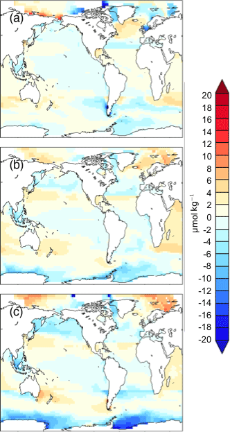
Figure A1 Shown is the difference between the exact DIC_dis surface field in µmol kg⁻¹, where DIC_sat has been calculated using the surface alkalinity ($\mathrm{alk}[z=\mathrm{0}]={\mathrm{alk}}_{\mathrm{pre}}[z=\mathrm{0}]$) and ${\mathrm{DIC}}_{\mathrm{soft}}[z=\mathrm{0}]={\mathrm{DIC}}_{\mathrm{carb}}[z=\mathrm{0}]=\mathrm{0}$. Differences are shown for (a) cold world; (b) moderate world; (c) hot world.