The effect of the 2013–2016 high temperature anomaly in the subarctic Northeast Pacific (the “Blob”) on net community production

A large anomalously warm water patch (the “Blob”) appeared in the NE Pacific Ocean in the winter of 2013–2014 and persisted through 2016 causing strong positive upper ocean temperature anomalies at Ocean Station Papa (OSP, 50^∘ N, 145^∘ W). The effect of the temperature anomalies on annual net community production (ANCP) was determined by upper ocean chemical mass balances of O₂ and dissolved inorganic carbon (DIC) using data from a profiling float and a surface mooring. Year-round oxygen mass balance in the upper ocean (0 to 91–111 m) indicates that ANCP decreased after the first year when warmer water invaded this area and then returned to the “pre-Blob” value (2.4, 0.8, 2.1, and 1.6 mol C m⁻² yr⁻¹ from 2012 to 2016, with a mean value of 1.7±0.7 mol C m⁻² yr⁻¹). ANCP determined from the DIC mass balance has a mean value that is similar within the errors as that from the O₂ mass balance but without a significant trend (2.0, 2.1, 2.6, and 3.0 mol C m⁻² yr⁻¹ with a mean value of 2.4±0.6 mol C m⁻² yr⁻¹). This is likely due to differences in the air–sea gas exchange, which is a major term for both mass balances. Oxygen has a residence time with respect to gas exchange of about 1 month while the CO₂ gas exchange response time is more like a year. Therefore the biologically induced oxygen saturation anomaly responds fast enough to record annual changes, whereas that for CO₂ does not. Phytoplankton pigment analysis from the upper ocean shows lower chlorophyll a concentrations and changes in plankton community composition (greater relative abundance of picoplankton) in the year after the warm water patch entered the area than in previous and subsequent years. Our analysis of multiple physical and biological processes that may have caused the ANCP decrease after warm water entered the area suggests that it was most likely due to the temperature-induced changes in biological processes.

1 Introduction

Net community production (NCP) in the upper ocean is defined as net organic carbon production, which equals biological production minus respiration. At a steady state when integrated over a period of at least 1 year, the annual NCP (ANCP) is equivalent to the flux of biologically produced organic matter from the upper ocean to the interior. Both biological production and respiration processes are temperature-dependent, and heterotrophic activities such as community respiration and zooplankton grazing are usually considered to be more sensitive to temperature change than autotrophic production (Allen et al., 2005; Brown et al., 2004; Gillooly et al., 2001; López-Urrutia et al., 2006; Regaudie-De-Gioux and Duarte, 2012; Rose and Caron, 2007). This implies that rising temperature should lead to enhanced heterotrophy and lower NCP (López-Urrutia et al., 2006). In contrast, it has also been suggested (e.g., Chen and Laws, 2017) that the main effect of temperature on community metabolism is likely due to differences in phytoplankton community composition (e.g., cyanobacteria dominate in warm, oligotrophic waters, whereas diatoms dominate in cold, nutrient-rich areas) rather than to lower temperature sensitivity of phytoplankton production.

From the winter of 2013, a large anomalously warm water patch (the “Blob”) appeared in the NE Pacific Ocean (Bond et al., 2015). The Blob had stretched from Alaska to Baja California by the end of 2015 (Di Lorenzo and Mantua, 2016) and caused widespread changes in the marine ecosystem, such as geographical shifts of plankton species, harmful algal blooms, and strandings of fishes, marine mammals, and seabirds (Cavole et al., 2016; Peña et al., 2018). Here we calculate the ANCP with upper ocean oxygen (O₂) and dissolved inorganic carbon (DIC) mass balances using data from Ocean Station Papa in the NE Pacific (OSP, 50^∘ N, 145^∘ W; Fig. 1), to determine if there were significant NCP changes during the anomalous warm event. The monthly sea surface temperature anomaly (SSTA) at OSP from 2012 to 2016 (Fig. 2) indicates that for most of the first year (starting from June 2012) sea surface temperature (SST) was lower than usual, but then transitioned to a strong positive temperature anomaly from 2013 to 2014. The positive anomaly continued with a magnitude of ∼2 ^∘C to June 2015, and then dropped back to “normal” in the summer of 2016.

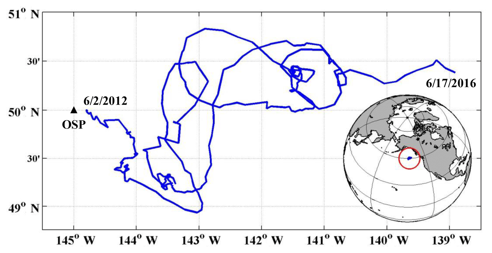
Figure 1 Study area and float path from 2012 to 2016. The black triangle indicates the position of Ocean Station Papa (OSP) mooring, and the blue line indicates the trajectory of the SOS-Argo float which was within roughly a 2^∘ (N–S) $\times \mathrm{6}{}^{\circ }$ (E–W) box.

Our field location is in the subarctic Northeast Pacific Ocean at OSP, where repeat hydrographic cruises have been carried out since 1981 by Fisheries and Oceans Canada with a frequency of two to three times per year (Freeland, 2007). A NOAA surface mooring has been deployed at OSP since 2007, for physical and biogeochemical measurements such as temperature, salinity, wind, ocean current, radiation, oxygen and total gas pressure, pH, and carbon dioxide (CO₂) (Emerson et al., 2011; Cronin et al., 2015; Fassbender et al., 2016). In addition, Argo profiling floats have been deployed near OSP since the 2000s (Freeland and Cummins, 2005). The first floats measured only temperature, salinity, and pressure but then measurements of oxygen and nitrate were added (Bushinsky and Emerson, 2015; Johnson et al., 2009). NCP at OSP has been determined using various approaches over the years, including bottle incubations (Wong, 1995), ²³⁴Th methods (Charette et al., 1999), carbon/nutrient drawdown (Fassbender et al., 2016; Plant et al., 2016; Takahashi et al., 1993; C. Wong et al., 2002; C. S. Wong et al., 2002b), and oxygen mass balance (Bushinsky and Emerson, 2015; Emerson, 1987; Emerson et al., 1991, 1993; Giesbrecht et al., 2012; Juranek et al., 2012; Plant et al., 2016).

2 Methods

2.1 Measurements of O₂, DIC, and phytoplankton biomass

Autonomous in situ oxygen measurements were made on a profiling float deployed by the University of Washington (Special Oxygen Sensor Argo float, SOS-Argo F8397, WMO no. 5903743; Fig. 1). The complete dataset is available at https://sites.google.com/a/uw.edu/sosargo/ (last access: 8 November 2018), and some of the data have been published previously by Bushinsky and Emerson (2015) and Yang et al. (2017). Oxygen measurements on the SOS-Argo float were obtained using an Aanderaa optode oxygen sensor with an air-calibration mechanism (Bushinsky et al., 2016) capable of providing the air–sea difference in oxygen concentration with an accuracy of about ±0.2 % and a vertical resolution of 3–5 m in the top 200 m of water column. This float was operated at a cycle interval of ∼5 days, covering depths from the surface to 1800 m.

Partial pressure of seawater CO₂ (pCO₂), temperature, and salinity data were obtained from the NOAA mooring at OSP (WMO no. 4800400). The complete dataset is available at https://www.nodc.noaa.gov/ocads/oceans/Moorings/Papa_145W_50N.html (last access: 8 November 2018), and some of the data were published by Fassbender et al. (2016). DIC was calculated using the total alkalinity (TA)–pCO₂ pair in CO2sys program Version 1.1 (van Heuven et al., 2011), where TA was calculated using the linear relationship with salinity developed in Fassbender et al. (2016) (TA $=\mathrm{37}\times S+\mathrm{988}$) for the OSP vicinity. The calculation was performed on the total pH scale using the carbonate dissociation constants ($K_{\mathrm{1}}^{\prime }$ and $K_{\mathrm{2}}^{\prime }$) of Lueker et al. (2000), the ${\mathrm{HSO}}_{\mathrm{4}}^{-}$ dissociation constant from Dickson et al. (1990), and the B_T∕S ratio from Lee et al. (2010). The DIC data were normalized to the annual mean salinity at OSP (32.5), to eliminate the influence from evaporation/dilution.

Water samples for phytoplankton abundance and community composition were collected at OSP during 14 Line P repeat hydrographic cruises aboard the CCGS John P. Tully from 2012 to 2016 (February, June, and August for each year). Phytoplankton biomass, measured as total chlorophyll a (chl a) concentrations, and the contribution of the main taxonomic groups of phytoplankton to chl a were determined from high-performance liquid chromatography (HPLC) measurements of phytoplankton pigment concentrations (chlorophylls and carotenoids; Zapata et al., 2000) followed by CHEMTAX v1.95 analysis (Mackey et al., 1996). Eight algal groups were included in the chemotaxonomic analysis: diatoms, haptophytes, chlorophytes, pelagophytes, prasinophytes, dinoflagellates, cryptophytes, and cyanobacteria. However, cryptophytes were not found since their biomarker pigment, alloxanthin, was not detected in any of our samples. Pigment ratios for each algal group were obtained from Higgins et al. (2011) and used as “seed” values for multiple trials (60 runs) from randomized starting points, as described by Wright et al. (2009). The same initial pigment ratios (Table 1a) were used in all cruises but each cruise was run separately to allow potential variations in the CHEMTAX optimization to be expressed. The ranges of final pigment ratios are given in Table 1b and the final ratios for each cruise are given in Peña et al. (2018). The six best solutions (those with the lowest residuals) were averaged for estimating the taxonomic abundances.

Table 1 Pigment:chl a ratios for eight algal groups: (a) CHEMTAX initial ratio matrix, and (b) ranges of final pigment ratios obtained by CHEMTAX on the pigment data.

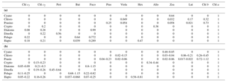
Abbreviations: Cyano, cyanobacteria; Chloro, chlorophytes; Prasino, prasinophytes; Crypto, cryptophytes; Dinofla, dinoflagellates; Pelago, pelagophytes; Hapto, haptophytes; Chl c₃, chlorophyll c₃; Chl c₂, chlorophyll c₂;
Peri, peridinin; But, 19'-butanoyloxyfucoxanthin; Fuco, fucoxanthin; Pras, prasinoxanthin; Viola, violaxanthin; Hex, 19'-hexanoyloxyfucoxanthin; Allo, alloxanthin; Zea, zeaxanthin; Lut, lutein; Chl b, chlorophyll b;
Chl a, chlorophyll.

2.2 Models used for NCP calculation

2.2.1 Oxygen mass balance model

Oxygen, temperature, and salinity data from SOS-Argo F8397 and wind speed (U₁₀) data from NOAA PMEL OSP mooring (https://www.pmel.noaa.gov/ocs/data/disdel/, last access: 8 November 2018, https://www.pmel.noaa.gov/ocs/data/fluxdisdel/, last access: 8 November 2018) were used in a multi-layer upper ocean O₂ mass balance model to calculate NCP. This model frame (Fig. 3) is similar to what was used in Bushinsky and Emerson (2015), which compartmentalizes the upper ocean (0–150 m) into a mixed layer box (with variable height) with 1 m boxes below. This model assumes that horizontal processes are not important. Because horizontal gradients of oxygen are small, lateral transport has much less influence on this property than fluxes from air–sea gas exchange, vertical advection, and diapycnal eddy diffusion. A detailed assessment of this assumption is given in Yang et al. (2017). Furthermore, the temperature time series measured by the SOS-Argo (Fig. S1 in the Supplement) shows no significant intrusions of fronts/eddies, and the continuity of water mass during the study period also allows us to use this simplified model that ignores horizontal processes.

Figure 2 Monthly SST anomaly at Ocean Station Papa (OSP). The anomaly is defined as the difference between the measured SST and the mean of 1971–2000. Data are from http://iridl.ldeo.columbia.edu/maproom/Global/Ocean_Temp/Anomaly.html (last access: 8 November 2018).

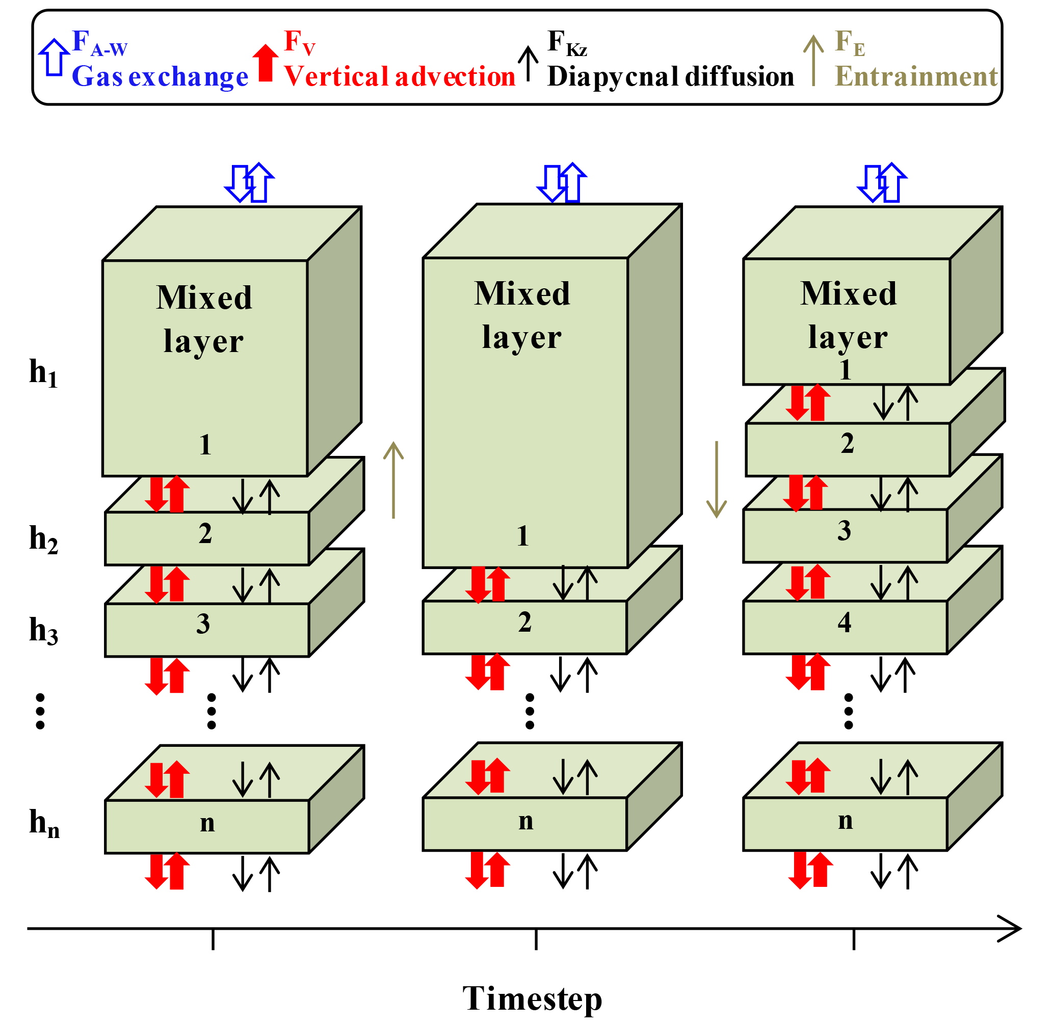
Figure 3 Schematic of the multi-layer upper ocean oxygen mass balance model (adapted from Bushinsky and Emerson, 2015). Fluxes (F) are from air–sea gas exchange (F_A−W, including diffusion and bubble processes), vertical advection (F_V), diapycnal eddy diffusion (F_Kz), and entrainment (F_E).

We define ANCP as the flux of organic carbon that escapes the upper ocean after a complete seasonal cycle. To be consistent with this definition, NCP is integrated vertically from the surface ocean to the winter mixed layer depth, which in this location is roughly equal to the pycnocline depth. Because internal waves cause a 10 to 20 m variation in the depth of density surfaces in this location, we used the annual mean pycnocline depth as the base of the modeled upper ocean to conserve mass in the model. Fluxes across the base of the upper ocean are calculated using measured gradients in oxygen at the density of the pycnocline, independent of its depth.

Oxygen concentration changes over time in the modeled upper ocean with depth of h (dh[O₂]∕dt) are the sum of gas exchange fluxes (F_A−W), vertical advection flux (F_V), diapycnal eddy diffusion (F_Kz), entrainment between the mixed layer and the water below (F_E), and net biological oxygen production (J_NCP).

$$\begin{array}{}\text{(1)}& {\displaystyle \frac{\mathrm{d}h\left[{\mathrm{O}}_{\mathrm{2}}\right]}{\mathrm{d}t}}=F_{\mathrm{A}-\mathrm{W}}+F_{\mathrm{V}}+F_{\mathrm{Kz}}+F_{\mathrm{E}}+J_{\mathrm{NCP}}\end{array}$$

F_A−W is only calculated for the mixed layer box, using a gas exchange model that includes both diffusion and bubble processes (Emerson and Bushinsky, 2016; Liang et al., 2013). With the time step (3 h) used in our case, the mixed layer change between time steps is always smaller than or equal to 1 m, so entrainment only occurs between the mixed layer box and the box below. The entrainment flux (F_E) that gets out of the mixed layer box ends up going into the box below and vice versa, so F_E values for these two boxes are the same but have different signs and cancel each other out. F_V is calculated from the Ekman pumping rate (derived from wind speed) and oxygen gradient from SOS-Argo measurements. F_Kz is calculated with the oxygen gradient and diapycnal eddy diffusion coefficient from Cronin et al. (2015), which decreases with depth from the base of the mixed layer to a background value of 10⁻⁵ m⁻² s⁻¹ (Whalen et al., 2012) with a 1∕e scaling described in Sun et al. (2013) (see also Bushinsky and Emerson, 2015). For the mixed layer reservoir F_kz and F_V are only considered at the base of the box. For all the boxes below the mixed layer, F_kz and F_V are considered both on the top and at the base of each box. Biological oxygen production, J_NCP, is the difference between the calculated fluxes and the measured time rate of change (left-hand side of Eq. 1). This value is converted from oxygen to carbon production (i.e., ANCP) using a constant oxygen to carbon ratio of 1.45 (Hedges et al., 2002).

The uncertainty of ANCP was estimated using a Monte Carlo approach. Confidence intervals for oxygen measurements and the gas exchange mass transfer coefficients used in the oxygen mass balance model were assigned to the model, and varied randomly while ANCP was calculated in 200 runs for each calculation. Details of this approach are presented in the Supplement and Yang et al. (2017).

2.2.2 DIC mass balance model

We used a similar mass balance model for DIC, in which the base of the modeled upper ocean is set to the annual mean pycnocline depth (the same as the oxygen mass balance model). This choice of the upper ocean depth distinguishes this model from the mixed layer model used in Fassbender et al. (2016). Fluxes at the base of the upper ocean in our model use DIC gradients, diapycnal eddy diffusion coefficients, and upwelling velocities determined at the mean pycnocline depth, while Fassbender et al. (2016) used the values at the bottom of the mixed layer. Because the OSP surface mooring only provided the mixed layer DIC data, we assumed that there is no annual net DIC change in the depth region between the mixed layer and the annual mean pycnocline depth. The depth gradient of DIC used to calculate fluxes across the pycnocline was calculated from measured oxygen gradients assuming a dO₂∕dz to dDIC∕dz ratio of 1.45 (Hedges et al., 2002). Thus, we assume for this calculation that the DIC change at the pycnocline depth is only due to degradation of organic matter, which ignores the change due to CaCO₃ dissolution (Fassbender et al., 2016). For the DIC mass balance the multi-layer model is equivalent to a one-layer model:

$$\begin{array}{}\text{(2)}& {\displaystyle \frac{\mathrm{d}h\left[\mathrm{DIC}\right]}{\mathrm{d}t}}=F_{\mathrm{A}-\mathrm{W}}+F_{\mathrm{V}}+F_{\mathrm{Kz}}+F_{\mathrm{E}}+J_{\mathrm{NCP}},\end{array}$$

where the DIC change (dh[DIC]∕dt) for the modeled upper ocean (the air–sea interface to the mean depth of the pycnocline) is due to air–water CO₂ exchange (F_A−W) at the air–sea interface, vertical advection (F_V) and diapycnal eddy diffusion (F_Kz) at the base of the modeled upper ocean, and net biological carbon production (J_NCP) in between. For this one-layer model, entrainment occurred within the same layer (box) and therefore there is no net entrainment flux (F_E=0). The air–sea gas exchange mass transfer coefficient is calculated as a function of wind speed using equations from Wanninkhof (2014). The DIC gradients used for F_V and F_Kz are derived from oxygen gradients at the pycnocline depth as described above.

2.3 Temperature dependence of NCP derived from the metabolic theory of ecology

The correlation between NCP variation and environmental temperature could be attributed to the temperature dependence of planktonic metabolism. Regaudie-De-Gioux and Duarte (2012) derived the temperature dependences of gross primary production (GPP) and community respiration (CR) using the metabolic theory of ecology and a large historical dataset on volumetric planktonic metabolism in different seasons and ocean regimes (1156 estimates of volumetric metabolic rates and the corresponding water temperature). Equations (3) and (4) below are their linear regressions between the natural logarithm of the specific metabolic rates (GPP∕chl a and CR∕Chl a) and the inverted water temperature (1/kT):

$$\begin{array}{}\text{(3)}& {\displaystyle }& {\displaystyle }\mathrm{Ln}{\displaystyle \frac{\mathrm{GPP}}{\mathrm{Chl}a}}=a_{\mathrm{p}}{\displaystyle \frac{\mathrm{1}}{kT}}+b_{\mathrm{p}}\text{(4)}& {\displaystyle }& {\displaystyle }\mathrm{Ln}{\displaystyle \frac{\mathrm{CR}}{\mathrm{Chl}a}}=a_{\mathrm{r}}{\displaystyle \frac{\mathrm{1}}{kT}}+b_{\mathrm{r}},\end{array}$$

where chl a is the chlorophyll a concentration, k is the Boltzmann constant, T is the environmental temperature in Kelvin, and a_p, b_p, a_r, and b_r are slopes and intercepts for each linear regression. The temperature dependence of GPP∕CR can be derived by combining Eqs. (3) and (4):

$$\begin{array}{}\text{(5)}& {\displaystyle \frac{\mathrm{GPP}}{\mathrm{CR}}}=\mathrm{EXP}\left[(a_{\mathrm{p}}-a_{\mathrm{r}}){\displaystyle \frac{\mathrm{1}}{kT}}+(b_{\mathrm{p}}-b_{\mathrm{r}})\right].\end{array}$$

Since the community respiration (CR) includes the respiration of both autotrophs and heterotrophs, NCP can be calculated as the difference between GPP and CR.

$$\begin{array}{}\text{(6)}& {\displaystyle }\mathrm{NCP}=\mathrm{GPP}-\mathrm{CR}=\mathrm{GPP}\left(\mathrm{1}-{\displaystyle \frac{\mathrm{1}}{\frac{\mathrm{GPP}}{\mathrm{CR}}}}\right)\end{array}$$

Combining Eqs. (5) and (6) gives us the NCP–temperature relationship.

$$\begin{array}{}\text{(7)}& {\displaystyle }\mathrm{NCP}=\mathrm{GPP}\left\{\mathrm{1}-{\displaystyle \frac{\mathrm{1}}{\mathrm{EXP}\left[\right(a_{\mathrm{p}}-a_{\mathrm{r}})\frac{\mathrm{1}}{kT}+(b_{\mathrm{p}}-b_{\mathrm{r}}\left)\right]}}\right\}\end{array}$$

3 Results

3.1 Oxygen and DIC measurements

The evolutions of density, oxygen concentration, and the oxygen anomaly in percent supersaturation ($\mathrm{\Delta }{\mathrm{O}}_{\mathrm{2}}=\left(\right[{\mathrm{O}}_{\mathrm{2}}]/[{\mathrm{O}}_{\mathrm{2}}{]}_{\mathrm{sat}}-\mathrm{1})\times \mathrm{100}$) determined by the profiling float at OSP from 2012 to 2016 are presented in Fig. 4a–c. The saturation concentration of oxygen ([O₂]_sat) was calculated using equations from Garcia and Gordon (1992, 1993). The thin black line indicates the mixed layer depth, which is defined by a density offset from the value at 10 m using a threshold of 0.03 kg m⁻³ (de Boyer Montégut, 2004). The thick blue line indicates the pycnocline with a density of σ_θ=25.8 kg m⁻³, which follows [O₂] gradients well (Fig. 4b). The white boxes indicate the modeled upper ocean for each year, in which the base of the modeled upper ocean is the mean pycnocline depth for each year. Oxygen in the mixed layer was supersaturated from mid-April to October/November, and near saturation or slightly undersaturated for the rest of the year (Fig. 4c).

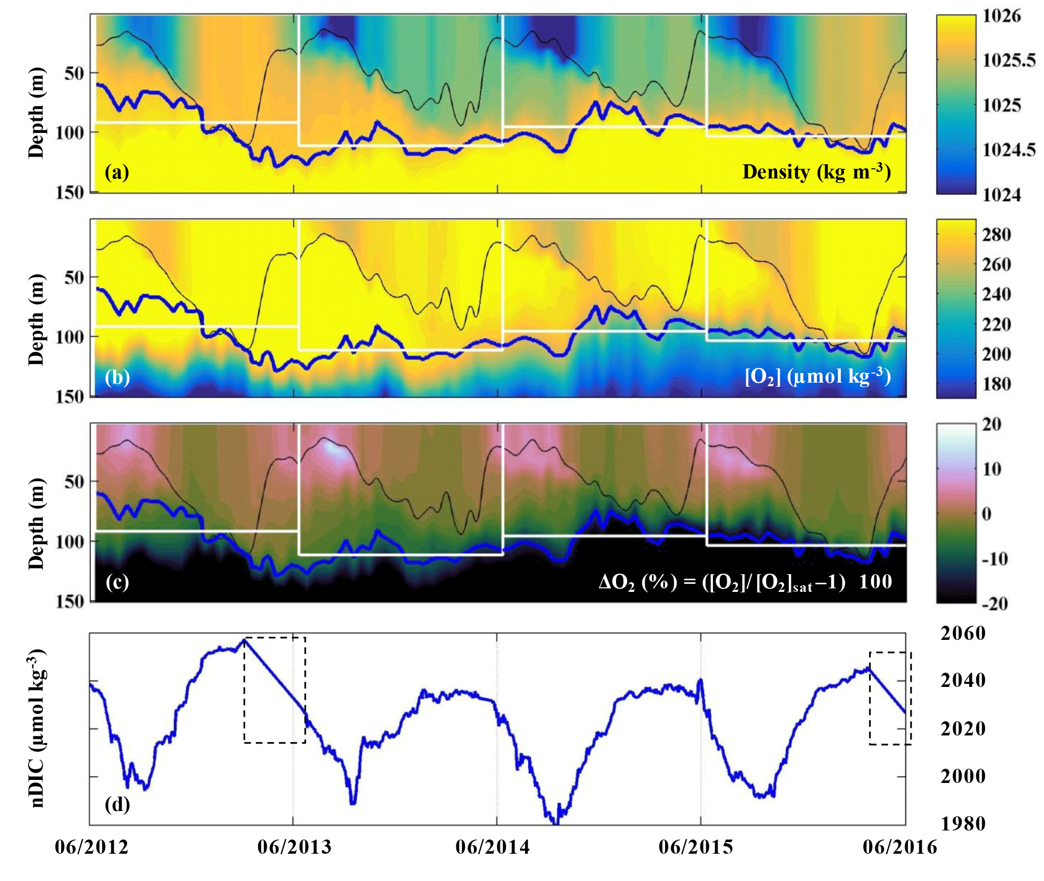
Figure 4 (a–c) Upper ocean density, oxygen concentration, and oxygen supersaturation ΔO₂ (%) from the SOS-Argo float at OSP. The thin black line indicates the mixed layer depth, the thick blue line indicates the pycnocline depth, and the white rectangles indicate the modeled upper ocean for each of the four years that ANCP was calculated. (d) Mixed layer DIC normalized to a surface salinity at OSP (S=32.5) from June 2012 to June 2016. Dashed line boxes indicate periods when the pCO₂ data were not available and thus were filled with a straight line interpolation.

The evolution of salinity normalized DIC in the mixed layer determined by the OSP mooring is presented in Fig. 4d. The pCO₂ sensor stopped working during two periods in 2013 and 2016 (indicated with dashed line boxes), and therefore the data for these two periods are filled with interpolated values. Strong summertime DIC drawdown was observed in each year, with the lowest DIC around September.

3.2 Annual net community production

All the terms of the oxygen mass balance calculation in each year are presented in Table 2a. The ANCP results (2.4±0.6, 0.8±0.4, 2.1±0.4 and 1.6±0.4 mol C m⁻² yr⁻¹, with a mean value of 1.7±0.7 mol C m⁻² yr⁻¹) indicate that ANCP initially decreased after warmer water invaded this area (2013–2014) and then returned to the “pre-Blob” value of 2012–2013 in subsequent years. Given the uncertainty in the estimate of ANCP in each year, the value during year 2013–2014 is significantly different at the 95 % confidence interval (as determined by a t test; Bethea et al., 1975). With the exception of the unusually low value for 2013–2014, ANCP values from oxygen mass balance calculation are very close to the historical ANCP estimates at OSP (2.3±0.6 mol C m⁻² yr⁻¹; Emerson, 2014).

Table 2 Annual net community production (ANCP) determined from (a) O₂ mass balance and (b) DIC mass balance. The annually integrated fluxes for each of the important terms (columns 4–9) indicate that the air–sea flux and biological production terms dominate for both tracers. Two ANCP values are given in (a): one integrated from the ocean surface to the depth of annual mean pycnocline (column 3), ANCP, and another value integrated over the depth of the mixed layer, ANCP_{mixed layer}. Only the former is a measure of the biological organic carbon that escapes the upper ocean on an annual basis (see text).

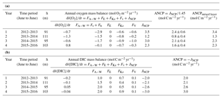
If we integrate the ANCP from the ocean surface to the depth of the mixed layer (ANCP_{mixed layer} in Table 2a) instead of to the annual mean depth of the pycnocline, the results are higher (3.4, 1.3, 2.3, and 2.3 mol C m⁻² yr⁻¹, with a mean value of 2.4±0.9 mol C m⁻² yr⁻¹). While the mean value is higher because it includes some organic carbon flux that is degraded between the mixed layer and pycnocline in summer, the annual trend, in which ANCP is significantly lower in year two (2013–2014), is the same as that in which ANCP values were determined for the depth interval above the pycnocline.

In comparison, ANCP values determined from the DIC mass balance are 2.0, 2.1, 2.6, and 3.0 mol C m⁻² yr⁻¹, with a mean value of 2.4±0.5 mol C m⁻² yr⁻¹ (Table 2b). The mean value is similar within the errors of the value determined from the oxygen mass balance (1.7±0.7 mol C m⁻² yr⁻¹) but there is no significant change between the second year (2013–2014) and those before and after. The somewhat higher value could be due to the assumption we made about DIC change below the mixed layer or because we neglected horizontal advection (see Discussion).

3.3 Phytoplankton abundance and community composition

Chl a concentration, an indicator of phytoplankton biomass, was about 50 % lower (0.22 mg m⁻³) during the period from August 2013 to June 2014 than during the rest of the 2012 to 2016 period (Fig. 5a) and the historical annual average at OSP (Peña and Varela, 2007). Chl a resumed to the 2012–2013 level in August 2014 and had a significant increase in the summer of 2016. 19'-hexanoyloxyfucoxanthin (Hex), which is mainly derived from prymnesiophytes, was found to be the most abundant pigment after T–chl a (Fig. 5b). Fucoxanthin (Fuco), a pigment associated with diatoms, haptophytes, and pelagophytes, was also abundant and showed increased concentration (0.54 mg m⁻³) in June 2016, coinciding with increased T–chl a. After Hex and Fuco, chlorophyll b was the most abundant pigment (0.36 to 0.27 mg m⁻³), indicating the presence of green algae. We also occasionally detected lutein (0–0.125 mg m⁻³), violaxanthin (0–0.012 mg m⁻³), and prasinoxanthin (0–0.005 mg m⁻³), which are biomarkers for green algae.

The CHEMTAX analysis detected the presence of seven classes of phytoplankton (Fig. 5c) and showed an increase in the relative contribution of cyanobacteria and chlorophytes during the Blob period, with the highest proportion of the former group in June of 2014 and the latter in June 2015 (Fig. 5c). There was also a decrease in the abundance of diatoms from August 2013 to June 2015. The remainder of the phytoplankton community was primarily composed of haptophytes and the contribution of the other phytoplankton groups was variable and showed no consistent year-to-year variability. By August 2015 the phytoplankton community had returned to a similar relative composition as observed in 2012–2013, with nanoplankton (mostly haptophytes) being dominant and with microplankton (diatoms and dinoflagellates) increasing in abundance. The input matrix (Table 1a) appeared to describe the environment well since the final pigment ratio matrix did not differ dramatically from the initial input values.

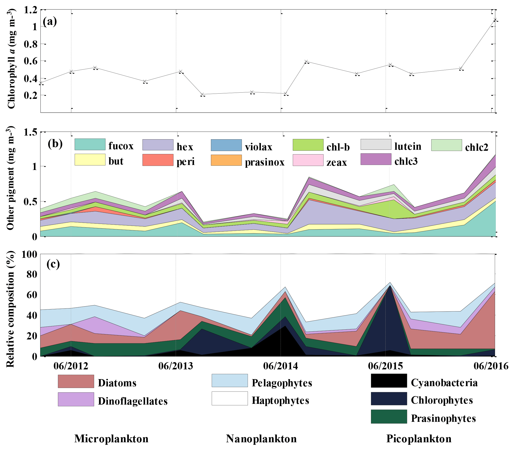
Figure 5 Mixed layer mean (a) chl a concentration (mg m⁻³), (b) other pigment concentration (mg m⁻³), and (c) relative phytoplankton composition (%) at OSP. Values were determined from HPLC pigment analysis of samples collected in February, June, and August for each year from 2012 to 2016.

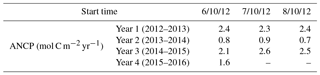
Table 3 ANCP calculated from O₂ mass balance with different start dates to determine if the chosen annual period affects the conclusions (see text).

4 Discussion

4.1 Comparisons of ANCP from oxygen and DIC mass balances

Although the ANCP is integrated to the same depth in our oxygen and DIC mass balance models, as mentioned in Sect. 3.2, the ANCP determined from the DIC mass balance (4-year mean: 2.4±0.5 mol C m⁻² yr⁻¹) is somewhat higher than the value determined from oxygen mass balance (4-year mean: 1.7±0.7 mol C m⁻² yr⁻¹), but still within the error of the model. There are two possible reasons for such discrepancy. First of all, due to the lack of DIC data below the mixed layer, for the DIC model we made an assumption that there is no annual net DIC change in the depth region between the mixed layer and the annual mean pycnocline depth. With this assumption, the ANCP from the DIC mass balance is higher because it includes the organic carbon that is degraded between the mixed layer and pycnocline in summer, so the ANCP from the DIC mass balance (4-year mean: 2.4±0.5 mol C m⁻² yr⁻¹) is very similar to the mixed layer ANCP determined from our oxygen mass balance model (4-year mean: 2.4±0.9 mol C m⁻² yr⁻¹) and the mixed layer ANCP determined by Fassbender et al. (2016) (2±1 mol C m⁻² yr⁻¹). The second possible reason that the 4-year mean value of ANCP determined from the DIC mass balance is higher than the value determined from the oxygen mass balance is horizontal advection. Because gas exchange resets the oxygen saturation anomaly for oxygen about 10 times faster than CO₂, the DIC mass balance is more vulnerable to horizontal fluxes than the O₂ mass balance. If we assumed that the difference in ANCP estimated from these two tracers (0.7 mol C m⁻² yr⁻¹) is due to horizontal advection, and calculate the horizontal DIC gradient using the 4-year mean horizontal velocity at OSP of 0.08 m s⁻¹, we found that a horizontal DIC gradient of $\mathrm{1}\times {\mathrm{10}}^{-\mathrm{8}}$ mol m⁻⁴ is required to cause the difference of 0.7 mol C m⁻² yr⁻¹, which is possible at this location (horizontal DIC gradient along the 4-year mean horizontal flow at OSP is about 2–$\mathrm{3}\times {\mathrm{10}}^{-\mathrm{8}}$ mol m⁻⁴ from GLODAP v1.1 gridded product; Key et al., 2004).

As for the interannual changes in ANCP, the oxygen mass balance calculation shows that ANCP had a significant decrease in 2013–2014 and then returned to the pre-Blob level in the following years, whereas ANCP calculated from the DIC mass balance does not show this trend. Since air–sea exchange is a large part of the flux mass balance for both oxygen and CO₂ (Table 2), a likely reason for this discrepancy is due to the shorter residence time with respect to gas exchange for the oxygen compared to the CO₂ saturation anomalies. An example of the residence time calculation is included in the Supplement, which indicates that the gas exchange residence time in the upper ocean for oxygen is about 1 month and that for CO₂ is about 1 year (see also Emerson and Hedges, 2008, chap. 11). Thus, the biologically induced saturation anomaly for oxygen responds fast enough to record annual changes, whereas that for pCO₂ and DIC does not. On the other hand, as discussed above, since DIC mass balance is more vulnerable to horizontal flux than oxygen mass balance, the DIC signal might have already been “smoothed” by the horizontal flux, which may also explain why the interannual ANCP changes were not observed when using the DIC mass balance approach. Alternatively, the production ratio of particulate organic carbon (POC) and particulate inorganic carbon (PIC) may cause the interannual variation of DIC mass balance. However, in our case since there was no significant bloom of haptophytes (e.g., coccolithophore) during the study period (Fig. 5c), it is unlikely that the interannual change in POC ∕ PIC ratio would affect the ANCP result calculated from the DIC mass balance. Hence, from this point forward we will focus on analyzing the factors that might influence ANCP variations determined with the oxygen mass balance model.

4.2 Causes of ANCP decrease

In the following paragraphs, we analyze connections between ANCP decrease and the Blob temperature anomaly in the context of multiple physical and biological processes, including the choices of start time from which ANCP are calculated, the base depth of the modeled upper ocean, planktonic metabolism, and changes in phytoplankton community composition.

Our observations began in June 2012, 10–12 months before the positive SST anomalies. To determine whether the start date for determining the ANCP values affects the results, we began the time series in four different months (Table 3). We are somewhat limited because there are only about 12 pre-Blob months before June 2012. However, as shown in Table 3, as long as there are more pre-Blob months than “Blob-affected” months in the first year, the significant ANCP decrease from the first to the second year is still observed and the trend of ANCP variation for those 4 years remains.

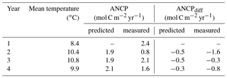
Table 4 Comparisons of ANCP measured with O₂ mass balance and ANCP predicted from the temperature dependence parameterization of planktonic metabolism using parameters from the Arctic Ocean (Regaudie-De-Gioux and Duarte, 2012). Gross primary production (GPP) is calculated from ANCP in the first year and Eq. (7), and it is assumed to be the same through years 1–4. ANCP_diff=2.4 (mol C m⁻² yr⁻¹) – ANCP_{predicted or measured}.

To determine whether the annual mean pycnocline depth (the white rectangles in Fig. 4a–c) influences the ANCP trends, we calculated ANCP using the 4-year mean depth of 100 m for the modeled upper ocean. The ANCP results only change slightly (2.6, 1.0, 1.9, and 1.6 mol C m⁻² yr⁻¹) and the decrease in 2013–2014 is still statistically significant, indicating that the different base depth used for the modeled upper ocean is not the key factor that causes ANCP changes.

To test if the temperature dependence of planktonic metabolism is strong enough to cause the ANCP decline we observed (e.g., 1.6 mol C m⁻² yr⁻¹ between 2012–2013 and 2013–2014), we calculated the GPP from measured NCP of the first year (2012–2013) using Eq. (7), and assumed GPP was constant for all four years so we could then determine the effect of temperature on NCP based on the metabolic theory of ecology (Eq. 7). Since the specific phytoplankton growth rate increases with increasing temperature (e.g., Regaudie-De-Gioux and Duarte, 2012; Chen and Laws, 2017), if phytoplankton biomass had remained the same during the Blob, GPP would have increased. Thus, assuming a constant GPP in this calculation is somewhat speculative, but it at least provides a first-order assessment of the metabolic temperature effect on ANCP. The parameterizations derived with datasets from the Arctic were used (Regaudie-De-Gioux and Duarte, 2012) because it gives the largest change in ANCP. The results (Table 4) indicate that the temperature dependence of planktonic metabolism is not strong enough to account for the measured ANCP decrease in the second year (2013–2014), suggesting that this is not the major reason for the observed ANCP decline.

Having ruled out the above likely candidates, we suggest that the observed ANCP decrease is most likely linked to the changes in GPP (e.g., low phytoplankton biomass observed in the second year; Fig. 5a) and phytoplankton community composition (Fig. 5c). In general, larger phytoplankton (i.e., microplankton) are more efficient exporters than smaller nanoplankton and picoplankton (e.g., Chen and Laws, 2017). Given the lower export rates of picoplankton (e.g., cyanobacteria) than those of larger phytoplankton (e.g., diatoms), the observed changes in phytoplankton community composition (Fig. 5b) in 2013–2014, which included a decrease in the relative abundance of diatoms, and an increase in the relative abundance of cyanobacteria and green algae (chlorophytes), could have further contributed to the decrease in ANCP. After the initial response to the temperature anomaly, chl a concentration and the phytoplankton community composition returned to levels similar to those observed before the warming occurred, suggesting that the plankton community rapidly adapted to the higher temperature and prevailing environmental conditions. These changes in GPP and phytoplankton community composition could be ultimately in response to the lack of micronutrients like iron (due to enhanced stratification from the Blob that restricted the vertical supply), which has been shown to regulate phytoplankton biomass and composition in this high-nutrient, low-chlorophyll region (e.g., Hamme et al., 2010; Marchetti et al., 2006). Unfortunately, we do not have iron data available to confirm that at this time.

5 Conclusions

The annual net community production (ANCP) at Ocean Station Papa (OSP) in the subarctic Northeast Pacific Ocean was determined from June 2012 to June 2016 to examine the effect of the temperature anomaly on the efficiency of carbon export. The ANCP determined with oxygen mass balance had a 4-year mean value of 1.7±0.7 mol C m⁻² yr⁻¹, whereas ANCP determined with DIC mass balance gives a somewhat higher mean value (2.4±0.5 mol C m⁻² yr⁻¹). ANCP for individual years determined from O₂ mass balance showed a significant decrease in the second year (2013–2014) after the onset of the temperature anomaly, but no significant decrease in ANCP was found when calculated with DIC mass balance. We believe that this indicates that the DIC concentration and pCO₂ respond too slowly to capture annual changes in ANCP. Based on our observations and historical ANCP estimates at OSP as reference, we found there was a significant ANCP decrease in 2013–2014 due to the warm anomaly, which is consistent with the findings from concurrent phytoplankton data. Possible mechanisms for the observed decrease in ANCP with the oxygen mass balance in the second year were analyzed in the context of multiple physical and biological processes that could be affected by the temperature anomaly. Our analysis showed that the ANCP decrease, as well as changes in phytoplankton abundance and community composition, was most likely due to changes in GPP after the Blob entered the area. These changes could be ultimately in response to the lack of micronutrients like iron during the Blob period. However, the ultimate cause cannot be specified by our analysis at this time.