the Creative Commons Attribution 4.0 License.
the Creative Commons Attribution 4.0 License.
 | 15 Jun 2020
Is there warming in the pipeline? A multi-model analysis of the Zero Emissions Commitment from CO2
Thomas L. Frölicher
Chris D. Jones
Joeri Rogelj
H. Damon Matthews
Kirsten Zickfeld
Vivek K. Arora
Noah J. Barrett
Victor Brovkin
Friedrich A. Burger
Micheal Eby
Alexey V. Eliseev
Tomohiro Hajima
Philip B. Holden
Aurich Jeltsch-Thömmes
Charles Koven
Nadine Mengis
Laurie Menviel
Martine Michou
Igor I. Mokhov
Akira Oka
Jörg Schwinger
Roland Séférian
Gary Shaffer
Andrei Sokolov
Kaoru Tachiiri
Jerry Tjiputra
Andrew Wiltshire
Tilo Ziehn
The Zero Emissions Commitment (ZEC) is the change in global mean temperature expected to occur following the cessation of net CO2 emissions and as such is a critical parameter for calculating the remaining carbon budget. The Zero Emissions Commitment Model Intercomparison Project (ZECMIP) was established to gain a better understanding of the potential magnitude and sign of ZEC, in addition to the processes that underlie this metric. A total of 18 Earth system models of both full and intermediate complexity participated in ZECMIP. All models conducted an experiment where atmospheric CO2 concentration increases exponentially until 1000 PgC has been emitted. Thereafter emissions are set to zero and models are configured to allow free evolution of atmospheric CO2 concentration. Many models conducted additional second-priority simulations with different cumulative emission totals and an alternative idealized emissions pathway with a gradual transition to zero emissions. The inter-model range of ZEC 50 years after emissions cease for the 1000 PgC experiment is −0.36 to 0.29 ∘C, with a model ensemble mean of −0.07 ∘C, median of −0.05 ∘C, and standard deviation of 0.19 ∘C. Models exhibit a wide variety of behaviours after emissions cease, with some models continuing to warm for decades to millennia and others cooling substantially. Analysis shows that both the carbon uptake by the ocean and the terrestrial biosphere are important for counteracting the warming effect from the reduction in ocean heat uptake in the decades after emissions cease. This warming effect is difficult to constrain due to high uncertainty in the efficacy of ocean heat uptake. Overall, the most likely value of ZEC on multi-decadal timescales is close to zero, consistent with previous model experiments and simple theory.
Please read the corrigendum first before continuing.
-
Notice on corrigendum
The requested paper has a corresponding corrigendum published. Please read the corrigendum first before downloading the article.
-
Article
(3890 KB)
-
The requested paper has a corresponding corrigendum published. Please read the corrigendum first before downloading the article.
- Article
(3890 KB) - Full-text XML
- Corrigendum
- BibTeX
- EndNote


The long-term temperature goal of the Paris Agreement is to hold global warming well below 2 ∘C and to endeavour to keep warming to no more than 1.5 ∘C (United Nations, 2015). An important metric to assess the feasibility of this target is the “remaining carbon budget” (e.g. Rogelj et al., 2018), which represents the total quantity of CO2 that can still be emitted without causing a climate warming that exceeds the temperature limits of the Paris Agreement (e.g. Rogelj et al., 2019a). The remaining carbon budget can be estimated from five factors: (1) historical human-induced warming to date, (2) the Transient Climate Response to cumulative CO2 emissions (TCRE), (3) the estimated contribution of non-CO2 climate forcings to future warming, (4) a correction for the feedback processes presently unrepresented by Earth System Models (ESMs), and (5) the unrealized warming from past CO2 emissions, called the Zero Emissions Commitment (ZEC) (e.g. Rogelj et al., 2019a). Of these five factors, ZEC is the only quantity whose uncertainty was not formally assessed in the recent Intergovernmental Panel on Climate Change (IPCC) Special Report on 1.5 ∘C. Here we present the results of a multi-model analysis that uses the output of dedicated model experiments that were submitted to the Zero Emissions Commitment Model Intercomparison Project (ZECMIP). This intercomparison project explicitly aims to quantify the ZEC and identify the processes that affect its magnitude and sign across models (Jones et al., 2019).
ZEC is the change in global temperature that is projected to occur following a complete cessation of net CO2 emissions (Matthews and Weaver, 2010). After emissions of CO2 cease, carbon is expected to be redistributed between the atmosphere, ocean, and land carbon pools, such that the atmospheric CO2 concentration continues to evolve over centuries to millennia (e.g. Maier-Reimer and Hasselmann, 1987; Cao et al., 2009; Siegenthaler and Joos, 1992; Sarmiento et al., 1992; Enting et al., 1994; Archer and Brovkin, 2008; Archer et al., 2009; Eby et al., 2009; Joos et al., 2013). In parallel, ocean heat uptake is expected to decline as the ocean comes into thermal equilibrium with the elevated radiative forcing (Matthews and Caldeira, 2008). In previous simulations of ZEC, the carbon cycle has acted to remove carbon from the atmosphere and counteract the warming effect from the reduction in ocean heat uptake, leading to values of ZEC that are close to zero (e.g. Plattner et al., 2008; Matthews and Caldeira, 2008; Solomon et al., 2009; Frölicher and Joos, 2010; Gillett et al., 2011). In the recent assessment of ZEC in the IPCC Special Report on Global Warming of 1.5 ∘C, the combined available evidence indicated that past CO2 emissions do not commit to substantial further global warming (Allen et al., 2018). A ZEC of zero was therefore applied for the computation of the remaining carbon budget for the IPCC 1.5 ∘C Special Report (Rogelj et al., 2018). However, the evidence available at that time consisted of simulations from only a relatively small number of models using a variety of experimental designs. Furthermore, some recent simulations have shown a more complex evolution of temperature following cessation of emissions (e.g. Frölicher et al., 2014; Frölicher and Paynter, 2015). Thus, a need to assess ZEC across a wider spectrum of climate models using a unified experimental protocol has been articulated (Jones et al., 2019).
ZEC was one of the metrics that emerged from the development of ESMs at the turn of the 21st century (Hare and Meinshausen, 2006). The concept was first conceptualized by Hare and Meinshausen (2006) who used the Model for the Assessment of Greenhouse gas Induced Climate Change (MAGICC), a climate model emulator, to explore temperature evolution following a complete cessation of all anthropogenic emissions. Matthews and Caldeira (2008) introduced the CO2-only concept of ZEC which is used here. Their experiments used the intermediate-complexity University of Victoria Earth System Climate Model (UVic ESCM) to show that stabilizing global temperature would require near zero CO2 emissions. Plattner et al. (2008) used a wide range of different Earth System Models of Intermediate Complexity (EMICs), following a similar experiment, and found that ZEC is close to (or less than) zero. These initial results with intermediate-complexity models were subsequently supported by emission-driven ESM simulations (Lowe et al., 2009; Frölicher and Joos, 2010; Gillett et al., 2011). Zickfeld et al. (2013) quantified the ZEC under different scenarios and for a range of EMICs, but the resulting range is biased towards negative values, as slightly negative, instead of zero emissions, were prescribed in some models. Some recent ESM simulations indicate that climate warming may continue after CO2 emissions cease. For example, Frölicher and Paynter (2015) performed a simulation with the full ESM GFDL-ESM2M, where emissions cease after 2 ∘C of warming is reached. The simulations show some decades of cooling followed by a multi-centennial period of renewed warming resulting in an additional 0.5 ∘C of warming 1000 years after emissions cease.
Two studies have examined the underlying physical and biogeochemical factors that generate ZEC in detail. Ehlert and Zickfeld (2017) examine ZEC with a set of idealized experiments conducted with the UVic ESCM. The study partitioned ZEC into a thermal equilibrium component represented by the ratio of global mean surface air temperature anomaly to unrealized warming, and a biogeochemical equilibrium component represented by the ratio of airborne fraction of carbon to equilibrium airborne fraction of carbon. The study found that the thermal equilibrium component of ZEC is much greater than the biogeochemical equilibrium component, implying a positive warming commitment. Williams et al. (2017) examine ZEC using the theoretical framework developed by Goodwin et al. (2007). The framework allows for the calculation of equilibrium atmospheric CO2 concentration if the cumulative effect of the land carbon sink is known. The framework was applied to the same simulation that was conducted for Frölicher and Paynter (2015). The analysis showed that ZEC emerges from two competing contributions: (1) a decline in the fraction of heat taken up by the ocean interior leading to radiative forcing driving more surface warming and (2) uptake of carbon by the terrestrial biosphere and ocean system removing carbon from the atmosphere, causing a cooling effect. Both studies focused on the long-term value of ZEC after multiple centuries, and thus neither study examined what drives ZEC in the policy-relevant time frame of a few decades following the cessation of emissions.
While we focus here on the ZEC from CO2 emissions only, the ZEC concept has also been applied to the climate commitment resulting from other greenhouse gas emissions and aerosols (Frölicher and Joos, 2010; Matthews and Zickfeld, 2012; Mauritsen and Pincus, 2017; Allen et al., 2018; Smith et al., 2019), wherein the ZEC is characterized by an initial warming due to the removal of aerosol forcing, followed by a more gradual cooling from the decline in non-CO2 greenhouse gas forcing. The ZEC from all emissions over multiple centuries is generally consistent with ZEC from only CO2 emissions for moderate future scenarios (Matthews and Zickfeld, 2012).
In addition to the ZEC, other definitions of warming commitment have also been used in the literature. The “constant composition commitment” is defined as the unrealized warming that results from constant atmospheric greenhouse gas and aerosol concentrations (Wigley, 2005; Meehl et al., 2005; Hare and Meinshausen, 2006). This variety of warming commitment was highlighted prominently in the 2007 IPCC report (Meehl et al., 2007), leading to a widespread misunderstanding that this additional “warming in the pipeline” was the result of past greenhouse gas emissions. However, the constant composition commitment instead results primarily from the future CO2 and other emissions that are required to maintain stable atmospheric concentrations over time (Matthews and Weaver, 2010; Matthews and Solomon, 2013). Another related concept is the future “emissions commitment” which quantifies the committed future CO2 (and other) emissions that will occur as a result of the continued operation of existing fossil fuel infrastructure (Davis et al., 2010; Davis and Socolow, 2014; Smith et al., 2019; Tong et al., 2019). This concept is also distinct from the ZEC, as it quantifies an aspect of socioeconomic inertia (rather than climate inertia), which has been argued to be an important driver of potentially unavoidable future climate warming (Matthews and Solomon, 2013; Matthews, 2014).
When considering climate targets in the range of 1.5 to 2.0 ∘C and accounting for the approximately 1 ∘C of historical warming to date (Allen et al., 2018; Rogelj et al., 2018), a ZEC on the order of ±0.1 ∘C can make a large difference in the remaining carbon budget. Hence, there is a need for a precise quantification and in-depth understanding of this value. This can be achieved via a systematic assessment of ZEC across the range of available models and a dedicated analysis of the factors that control the value of ZEC in these simulations. Thus, the goals of this study based on the simulations of the Zero Emissions Commitment Model Intercomparison Project (ZECMIP) are (1) to estimate the value of ZEC in the decades following cessation of emissions in order to facilitate an estimate of the remaining carbon budget, (2) to test if ZEC is sensitive to the pathway of emissions, (3) to establish whether ZEC is dependent on the cumulative total CO2 that are emitted before emissions cease, and (4) to identify which physical and biogeochemical factors control the sign and magnitude of ZEC in models.
The most policy-relevant question related to ZEC is whether global temperature will continue to increase following complete cessation of greenhouse gas and aerosol emissions. The present iteration of ZECMIP aims to answer part of this question by examining the temperature response in idealized CO2-only climate model experiments. To answer the question in full, the behaviour of non-CO2 greenhouse gases, aerosols, and land use change must be accounted for in a consistent way. Such efforts will be the focus of future iterations of ZECMIP.
2.1 Protocol and simulations
Here we summarize the ZECMIP protocol; the full protocol for ZECMIP is described in Jones et al. (2019). The ZECMIP protocol requested modelling groups to conduct three idealized simulations of two different types each: A and B. Type A simulations are initialized from one of the standard climate model benchmark experiments, in which specified atmospheric CO2 concentration increases at a rate of 1 % yr−1 from its pre-industrial value of around 285 ppm until quadrupling, referred to as the 1pctCO2 simulation in the Climate Model Intercomparison Project (CMIP) framework (Eyring et al., 2016). The three type A simulations are initialized from the 1pctCO2 simulation when diagnosed cumulative emissions of CO2 reach 750, 1000, and 2000 PgC. After the desired cumulative emission is reached, the models are set to freely evolving atmospheric CO2 mode, with zero further CO2 emissions. Since net anthropogenic emissions are specified to be zero in type A simulations, atmospheric CO2 concentration is expected to decline in these simulations in response to carbon uptake by the ocean and land. A consequence of the protocol is that for the type A simulations each model branches from the 1pctCO2 simulations in a different year, contingent on when a model reaches the target cumulative emissions, which in turn depends on each model's representation of the carbon cycle and feedbacks. An example of emissions for the type A experiments is shown in Fig. 1a. The three type B simulations are initialized from pre-industrial conditions and are emissions driven from the beginning of the simulation. Emissions follow bell-shaped pathways wherein all emissions occur within a 100-year window (Fig. 1b). In all experiments, land use change and non-CO2 forcings are held at their pre-industrial levels.
Due to the late addition of ZECMIP to the CMIP Phase 6 (CMIP6) (Eyring et al., 2016), only the 1000 PgC type A experiment (esm-1pct-brch-1000PgC) was designated as the top-priority ZECMIP simulation. The other simulations were designated as second-priority simulations and were meant to be conducted if participating modelling groups had the resources and time. Both full ESMs and EMICs were invited to participate in ZECMIP. ESMs were requested to perform the top-priority simulation for 100 years after CO2 emissions cease and more years and more experiments as resources allowed. EMICs were requested to conduct all experiments for at least 1000 years of simulations following cessation of emissions. Table 1 shows the experiments and experimental codes for ZECMIP.
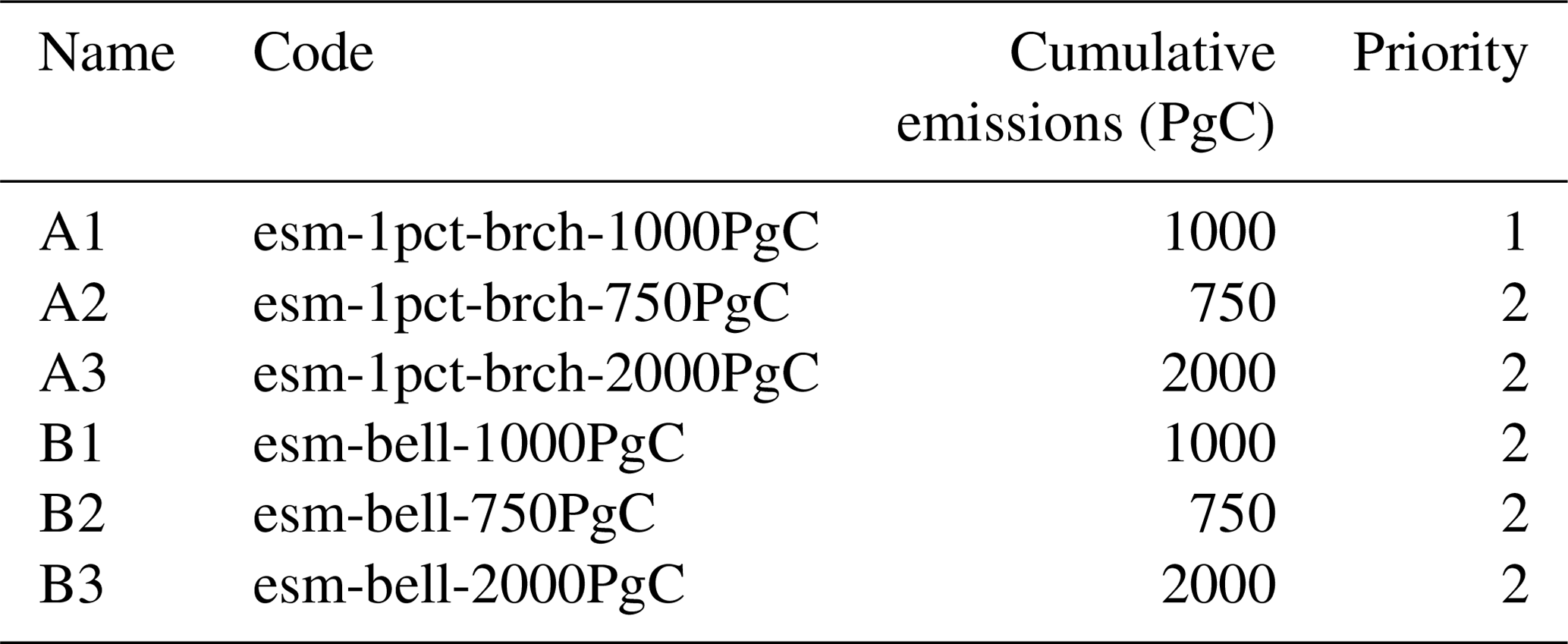
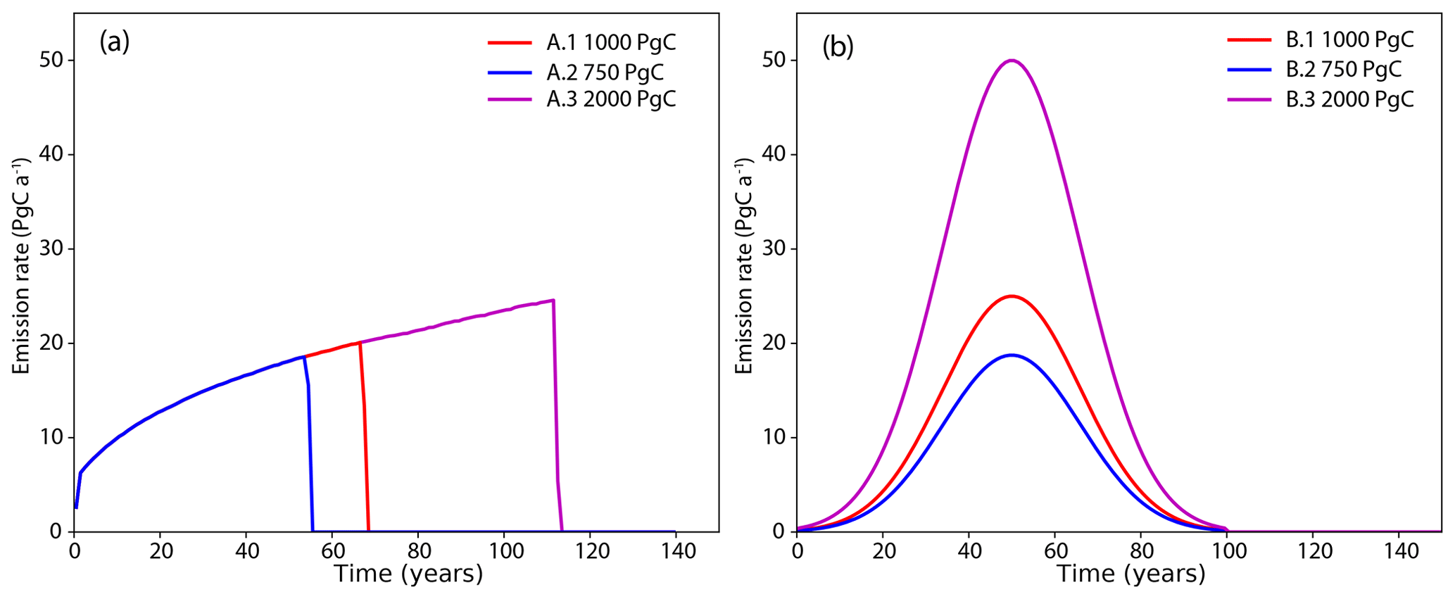
Figure 1(a) Example of diagnosed emission from the UVic ESCM for the type A experiments. Emissions are diagnosed from the 1pctCO2 experiment, which has prescribed atmospheric CO2 concentrations. The target cumulative emissions total is reached part way through the final year of emissions, thus the final year has a lower average emission rate than the previous year. (b) Time series of global CO2 emissions for bell curve pathways B1 to B3. The numbers in the legend indicate the cumulative amount of CO2 emissions for each simulation.
2.2 Model descriptions
A total of 18 models participated in ZECMIP: 9 comprehensive ESMs and 9 EMICs. The primary features of each model are summarized in Tables A1 and A2 in Appendix A. The ESMs in alphabetical order are the (1) CSIRO Australian Community Climate and Earth System Simulator, ESM version 1.5 – ACCESS-ESM1.5; (2) Canadian Centre for Climate Modelling and Analysis (CCCma), Canadian Earth System Model version 5 – CanESM5; (3) Community Earth System Model 2 – CESM2; (4) Centre National de Recherches Météorologiques (CNRM), CERFACS Earth System Model version 2 – CNRM-ESM2-1; (5) Geophysical Fluid Dynamics Laboratory (GFDL), Earth System Model version 2 – GFDL-ESM2M; (6) Japan Agency for Marine-Earth Science and Technology (JAMSTEC/team MIROC), Model for interdisciplinary Research on Climate, Earth System version 2, Long-term – MIROC-ES2L; (7) Max Planck Institute Earth System model, version 1.2, low resolution – MPI-ESM1.2-LR; (8) Norwegian Earth System Model 2 – NorESM2; and (9) United Kingdom (Met Office Hadley Centre and NERC), United Kingdom Earth System Model version 1 – UKESM1-0-LL. The nine EMICs in alphabetical order are the (1) Bern three-dimensional Earth System Model – Bern3D-LPX; (2) Climate–Biosphere model, version 2 – CLIMBER-2; (3) Danish Centre for Earth System Science Earth System Model – DCESS1.0; (4) A.M. Obukhov Institute of Atmospheric Physics, Russian Academy of Sciences – IAPRAS, (5) Loch-Vecode-ECbilt-Clio Model – LOVECLIM 1.2; (6) Massachusetts Institute of Technology Earth System Model – MESM; (7) Model for Interdisciplinary Research on Climate-lite/Japan Uncertainty Modelling Project Loosely Coupled Model – MIROC-lite; (8) Planet Simulator – Grid-Enabled Integrated Earth system model – PLASIM-GENIE; and (9) University of Victoria Earth System Climate Model version 2.10 – UVic ESCM 2.10. For brevity, these models are referred to by their short names for the remainder of the paper. Table 2 shows the ZECMIP experiments that each modelling group submitted.
Table 3 shows three benchmark climate metrics for each model: equilibrium climate sensitivity (ECS), transient climate response (TCR), and TCRE. ECS is the climate warming expected if atmospheric CO2 concentration was doubled from the pre-industrial value and maintained indefinitely while the climate system is allowed to come into equilibrium with the elevated radiative forcing (e.g. Planton, 2013; Charney et al., 1979). There are a variety of methods to compute ECS from climate model outputs (e.g. Knutti et al., 2017). Here we use ECS values computed using the method of Gregory et al. (2004), called “effective climate sensitivity”. The method of Gregory et al. (2004) computes ECS from the slope of the scatter plot between change in global temperature and planetary heat uptake, with values from the benchmark experiment where atmospheric CO2 concentration is instantaneously quadrupled (4×CO2 experiment). TCR is the atmospheric surface temperature change (relative to the pre-industrial temperature) when atmospheric CO2 is doubled in year 70 of the 1pctCO2 experiment, computed using a 20-year averaging window centred on year 70 of the experiment (e.g. Planton, 2013). TCRE is described in the introduction and is computed from year 70 of the 1 % experiment (e.g. Planton, 2013).
Bern and UVic submitted three versions of their models with three different ECSs. For Bern, these were ECSs of 2.0, 3.0, and 5.0 ∘C, and for UVic, these were ECSs of 2.0, 3.8, and 5.0 ∘C. These ECS values are true equilibrium climate sensitivities computed by allowing each model to come fully into equilibrium with the changed radiative forcing. For each model the central ECS value was used for the main analysis, i.e. 3.0 ∘C for Bern and 3.8 ∘C for UVic. The remaining experiments were used to explore the relationship between ECS and ZEC.
Table 2Experiments conducted for ZECMIP by model. Full ESMs are listed on top, followed by EMICs.
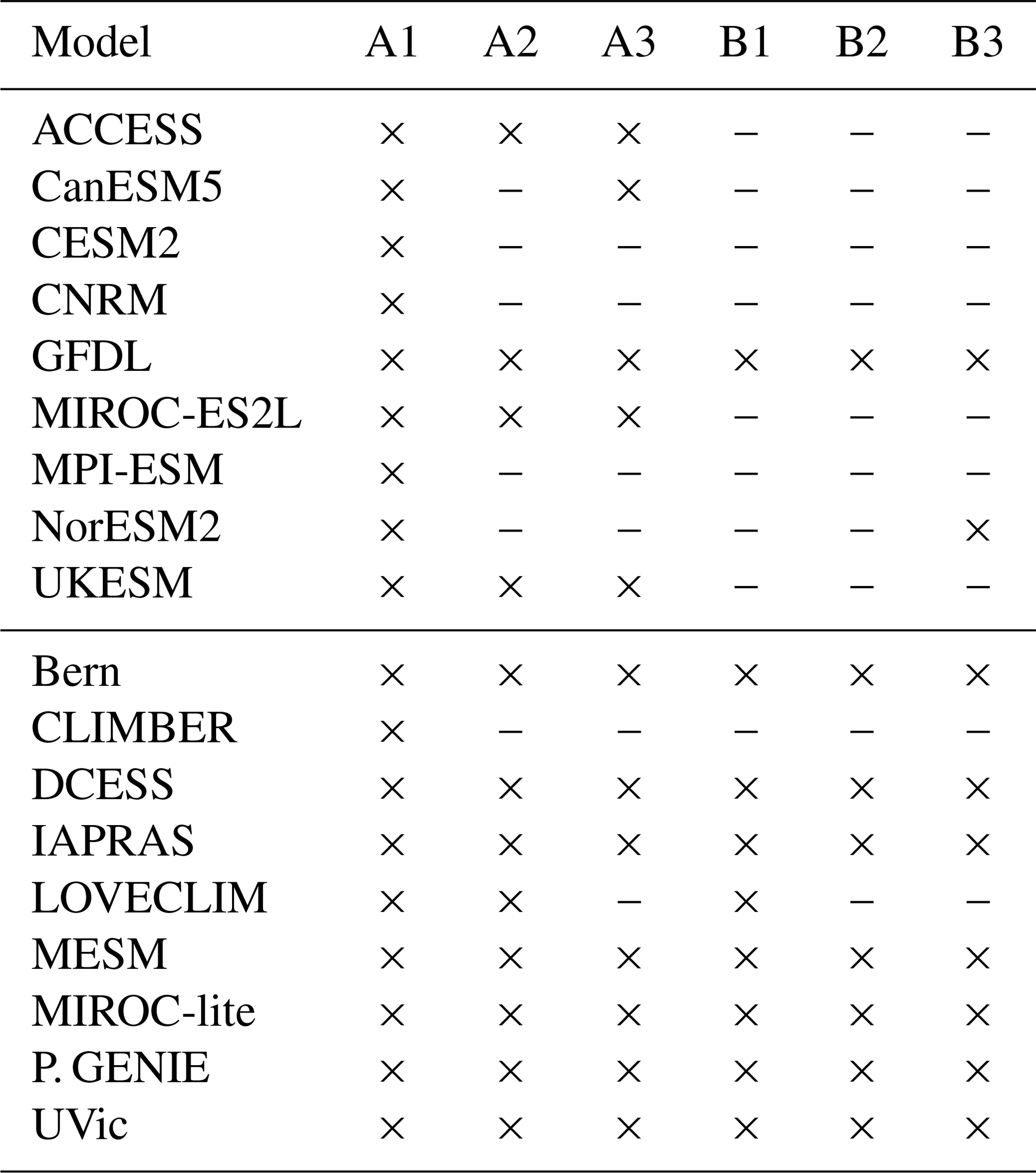
Table 3Benchmark climate model characteristics for each model: Equilibrium Climate Sensitivity (ECS), Transient Climate Response (TCR), and Transient Climate Response to Cumulative CO2 Emissions (TCRE). UKESM reported a maximum to minimum range for TCR and TCRE based on four ensemble members.

2.3 Quantifying ZEC
ZEC is the change in global average surface air temperature following the cessation of CO2 emissions. Thus, ZEC must be calculated relative to the global temperature when emissions cease. Typically such a value would be computed from a 20-year window centred on the year when emissions cease. However, for the ZECMIP type A experiments such a calculation underestimates the temperature of cessation, due to the abrupt change in forcing when emissions suddenly cease, leading to an overestimation of ZEC values. That is, a roughly linear increase in temperature pathway abruptly changes to a close to stable temperature pathway. Therefore, we define the temperature of cessation to be the global mean surface air temperature from the benchmark 1pctCO2 experiment averaged over a 20-year window centred on the year that emissions cease in the respective ZECMIP type A experiment (year the ZECMIP experiment branches from the 1 % experiment). For the EMICs which lack internal variability this method provides an unbiased estimate of the temperature of cessation.
Earlier studies have examined ZEC from decadal (Matthews and Zickfeld, 2012; Mauritsen and Pincus, 2017; Williams et al., 2017; Allen et al., 2018; Smith et al., 2019) to multi-centennial timescales (Frölicher and Paynter, 2015; Ehlert and Zickfeld, 2017). One of the main motivations of this present study is to inform the impact of the ZEC on the remaining carbon budget. This remaining carbon budget is typically used to assess the consistency of societal emissions pathways with the international temperature target of the Paris Agreement (UNEP, 2018). In this emission pathway and policy context, the ZEC within a few decades of emissions cessation is more pertinent than the evolution of the Earth system hundreds or thousands of years into the future. Therefore, we define values of ZECX as a 20-year average temperature anomaly centred at year X after emissions cease. Thus, 50-year ZEC (ZEC50) is the global mean temperature relative to the temperature of cessation averaged from year 40 to year 59 after emissions cease. We similarly define 25-year ZEC (ZEC25) and 90-year ZEC (ZEC90).
2.4 Analysis framework
A key question of the present study is why some models have positive ZEC and some models have negative or close to zero ZEC. From elementary theory we understand that the sign of ZEC will depend on the pathway of atmospheric CO2 concentration and ocean heat uptake following cessation of emissions (Wigley and Schlesinger, 1985). Complicating this dynamic is that atmospheric CO2 change has contributions both from the net carbon flux from the ocean and the terrestrial biosphere. Using the forcing response equation (Wigley and Schlesinger, 1985) and the common logarithmic approximation for the radiative forcing from CO2 (Myhre et al., 1998), we can partition ZEC into contributions from ocean heat uptake, ocean carbon uptake, and net carbon flux into the terrestrial biosphere. The full derivation of the relationship is shown in Appendix B, and the summary equations are shown below:
where λ (W m−2 K−1) is the climate feedback parameter, TZEC (K) is ZEC, R (W m−2) is the radiative forcing from an e-fold increase in atmospheric CO2 burden, t is time (a), ze is the time that emissions cease, fO (PgC a−1) is ocean carbon uptake, fL (PgC a−1) is carbon uptake by land, CA is atmospheric CO2 content (PgC), N is planetary heat uptake (W m−2), Nze is planetary heat uptake at the time emissions cease, and ϵ is the efficacy of planetary heat uptake. The equation states that ZEC is proportional to the sum of three energy balance terms: (1) the change in radiative forcing from carbon taken up by the ocean, (2) the change in radiative forcing from carbon taken up or given off by land, and (3) the change in effective ocean heat uptake. The two integral terms can be evaluated numerically from the ZECMIP model output and thus can be simplified into two energy forcing terms Focean and Fland:
and
and thus
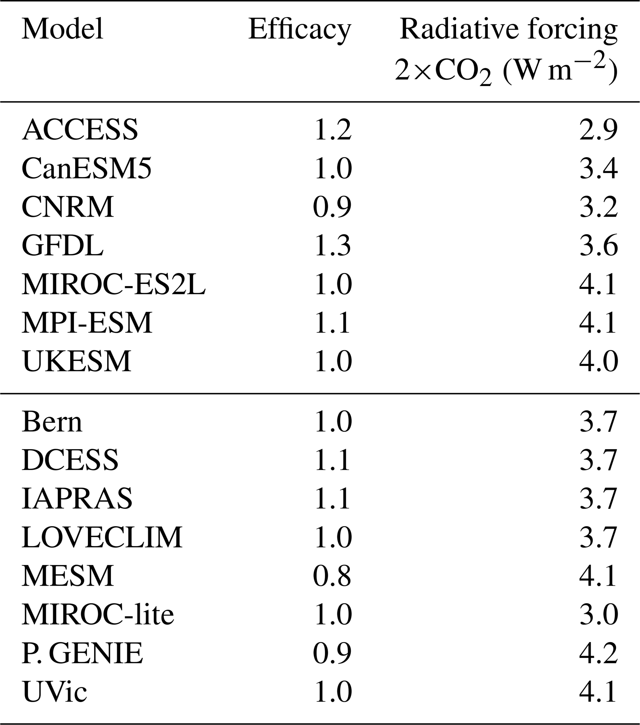
Values for R were computed from the effective radiative forcing value for the models that simulate internal variability, with effective radiative forcing provided by each modelling group. Bern, DCESS, and UVic prescribe exact values for R, and thus these values were used for calculations with these models. Effective radiative forcing for a doubling of CO2 is half the y intercept of a 4×CO2 Gregory plot (Gregory et al., 2004). R values and the effective climate sensitivities were used to calculate λ for each model. Efficacy (Winton et al., 2010) was calculated from the following equation:
where CAo (PgC) is the pre-industrial CO2 burden,and T (K) is the global mean temperature anomaly relative to pre-industrial temperature. T, N, and CA values were taken from the benchmark 1pctCO2 for each model as an average value from year 10 to year 140 of that experiment. Computed ϵ values are shown in Table 4. Effective climate sensitivity is calculated here as a time average fit and hence is assumed to be a constant, while efficacy values are expected to change in time. In CLIMBER, planetary or ocean heat uptake is not included into standard output and hence is not analyzed using this framework. CESM2 and NorESM2 are also excluded as the 4×CO2 experiment results for these models are not yet available.
Efficacy has been shown to arise from spatial patterns in ocean heat uptake (Winton et al., 2010, 2013; Rose et al., 2014), with ocean heat uptake in the high latitudes being more effective at cooling the atmosphere than ocean heat uptake in low latitudes (Rose et al., 2014). This spatial structure in the effectiveness of ocean heat uptake in turn is suspected to originate from shortwave radiation cloud feedbacks (Andrews et al., 2015). The method we have used to calculate efficacy folds state-dependent feedbacks and temporal change in the climate feedback parameter (Rugenstein et al., 2016) into the efficacy parameter.
Notably, calculated effective climate sensitivities and effective radiative forcings vary slightly within models due to the internal variability (Gregory et al., 2015), hence the efficacy values calculated here are associated with some uncertainty. Efficacy values are known to evolve in time (Winton et al., 2010); thus, the efficacy value from the 1pctCO2 experiment may be different than efficacy 50 years after emissions cease in the ZECMIP experiments. To test this effect yearly efficacy values were calculated for the four EMICs without internal variability (Bern, DCESS, MESM, and UVic). These tests showed that efficacy was 3.5 % to 25 % away from the values for the 1pctCO2 experiment 50 years after emissions cease (Fig. D1 in Appendix D). Thus, we have assigned efficacy a ±30 % uncertainty. Notably, efficacy declines in three of the four models, consistent with previous work showing strong trends in efficacy over time (Williams et al., 2017). Radiative forcing from CO2 is not precisely logarithmic (Gregory et al., 2015; Byrne and Goldblatt, 2014; Etminan et al., 2016), and therefore the calculated Focean and Fland values will be slightly different than the changes in radiative forcing experienced within each model, except for the three models that prescribe CO2 radiative forcing. Also accounting for the uncertainty in recovering R values from model output, we assign a ±10 % uncertainty to radiative forcing values.
Table 4Efficacy ϵ and radiative forcing for 2 × CO2 R values for each model. Efficacy values are calculated from the 1pctCO2 experiment.
3.1 A1 Experiment results
Figure 2 shows the evolution of atmospheric CO2 concentration and temperature for the 100 years after emissions cease for the A1 experiment (1 % branched at 1000 PgC). In all simulations atmospheric CO2 concentration declines after emissions cease, with a rapid decline in the first few decades followed by a slower decline thereafter. The rates of decline vary across the models. By 50 years after emissions cease in the A1 experiment, the change in atmospheric CO2 concentration ranged from −91 to −52 ppm, with a mean of −76 ppm and median of −80 ppm. Temperature evolution in the 100 years following cessation of emissions varies strongly by model, with some models showing declining temperature, others showing ZEC close to zero, and others showing continued warming following cessation of emissions. Some models, such as UKESM, CNRM, and UVic, exhibit continued warming in the centuries following cessation of emissions. Other models, such as IAPRAS and DCESS, exhibit a temperature peak and then decline. Still other models show ZECs that hold close to zero (e.g. MPI-ESM), while some models show continuous decline in temperature following cessation of emissions (e.g. P. GENIE). Table 5 shows the ZEC25, ZEC50, and ZEC90 values for the A1 experiment. The table shows values of ZEC50 ranging from −0.36 to 0.29 ∘C, with a model ensemble mean of −0.06 ∘C, median of −0.05 ∘C, and a standard deviation of 0.19 ∘C. Tables C1 and C2 show ZEC25, ZEC50, and ZEC90 for the A2 and A3 experiment. Figure 3 shows the evolution of atmospheric CO2 concentration, temperature anomalies (relative to the year that emissions cease), and ocean heat uptake for 1000 years following cessation of emissions in the A1 experiment. All models show continued decline in atmospheric CO2 concentration for centuries after emissions cease. One model (P. GENIE) shows a renewed growth in atmospheric CO2 concentration beginning about 600 years after emissions cease, resulting from release of carbon from soils overwhelming the residual ocean carbon sink. Of the nine models that extended simulations beyond 150 years, seven show temperature on a long-term decline (Bern, MESM, DCESS, IAPRAS, LOVECLIM, P. GENIE, and MIROC-ES2L), GFDL shows temperature declining and then increasing within 200 years after cessation but ultimately remaining close to the temperature at cessation, and the UVic model shows slow warming. Most models show continuous decline in ocean heat uptake with values approaching zero. Three models (GFDL, LOVECLIM and IAPRAS) show the ocean transition from a heat sink to a heat source.
Table 5Temperature anomaly relative to the year that emissions ceased, averaged over a 20-year time window centred on the 25th, 50th, and 90th year following cessation of anthropogenic CO2 emissions (ZEC25, ZEC50, and ZEC90, respectively) for the A1 (1 % to 1000 PgC experiment).
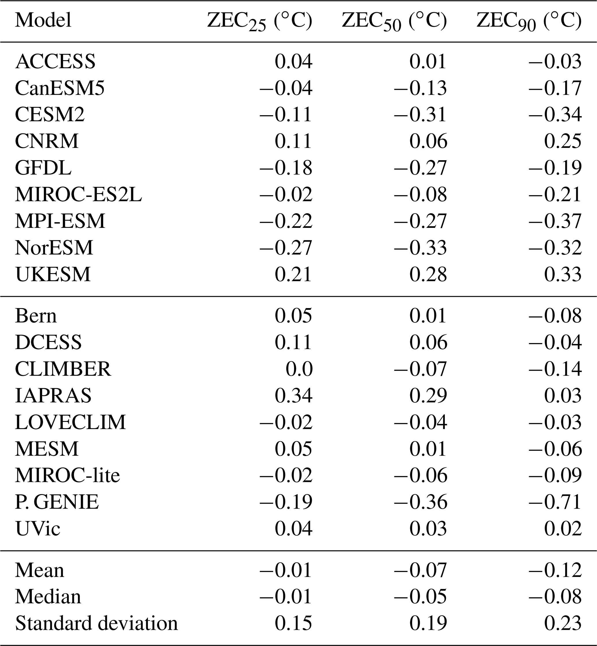
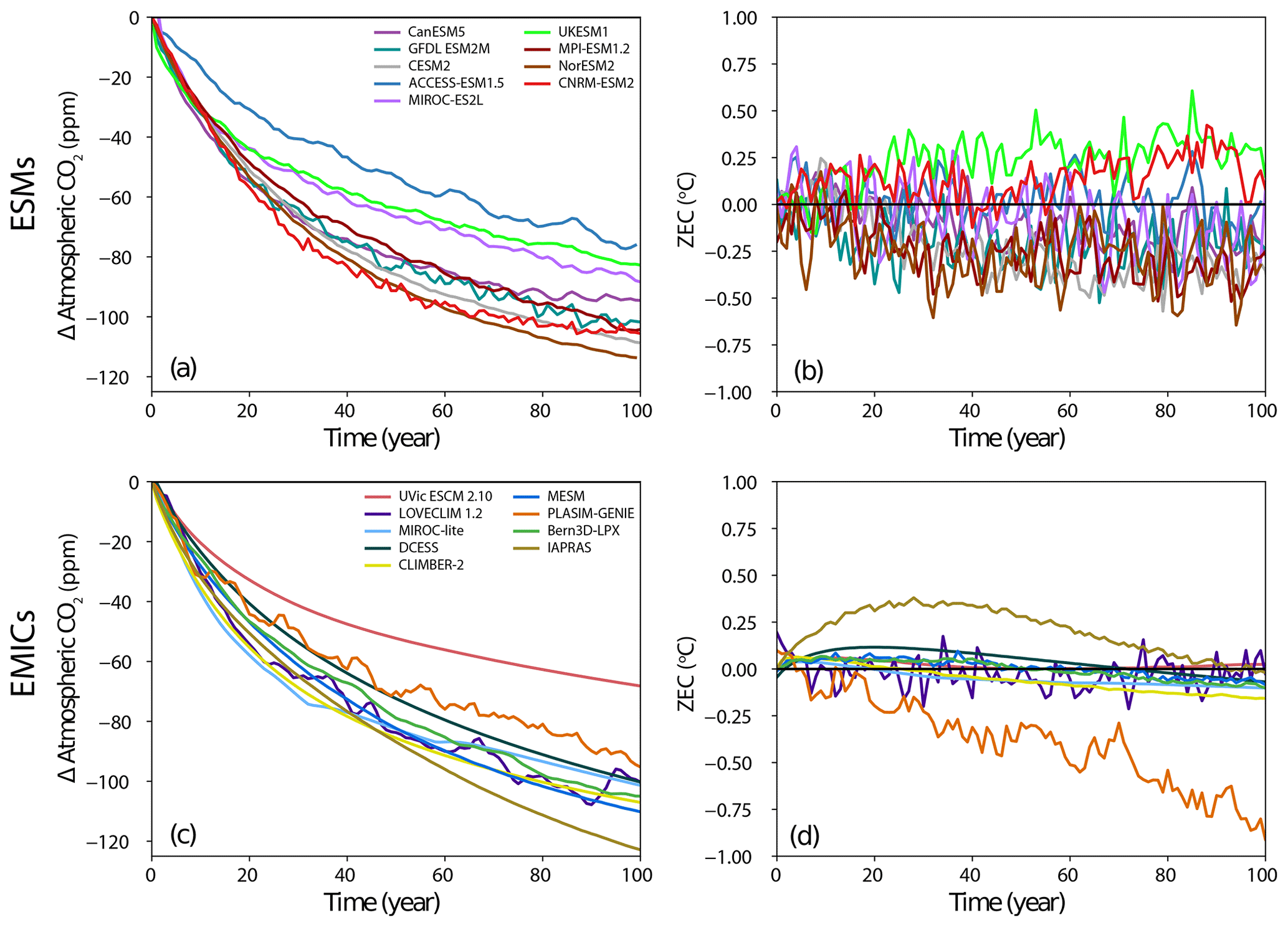
Figure 2(a, c) Atmospheric CO2 concentration anomaly and (b, d) Zero Emissions Commitment following the cessation of emissions during the experiment wherein 1000 PgC was emitted following the 1 % experiment (A1). ZEC is the temperature anomaly relative to the estimated temperature at the year of cessation. The top row shows the output for ESMs, and the bottom row shows the output for EMICs.
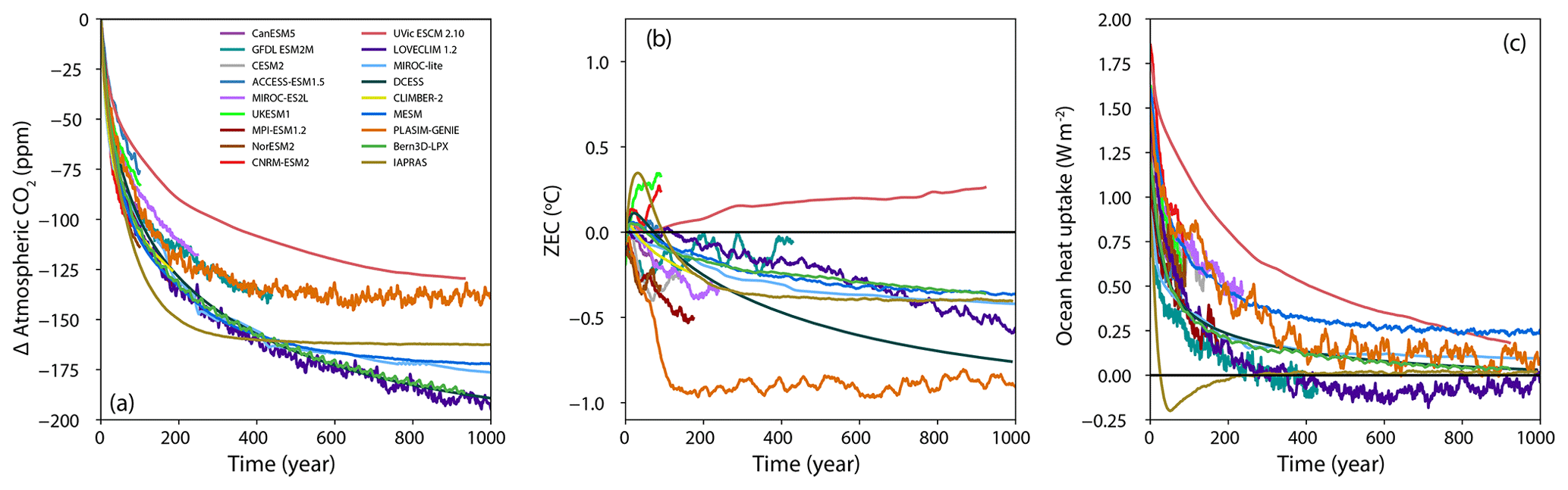
Figure 3(a) Change in atmospheric CO2 concentration, (b) change in temperature, and (c) ocean heat uptake following cessation of emissions for the A1 experiment (1000 PgC following 1 %) for 1000 years following the cessation of emissions.
3.2 Effect of emissions rate: 1 % vs. bell
The bell experiments were designed to test whether temperature evolution following cessation of emissions depends on the pathway of emissions before emissions cease. These experiments also illustrate model behaviour during a gradual transition to zero emissions (e.g. MacDougall, 2019), a pathway that is consistent with most future scenarios (Eyring et al., 2016). Nine of the participating models conducted both the A1 and B1 experiments, GFDL and eight of the EMICs (CLIMBER is the EMIC which did not conduct the B1 experiment). Figure 4 shows the temperature evolution (relative to pre-industrial temperature) for both experiments. All models show that by the 100th year of the experiments, when emissions cease in the bell experiment, the temperature evolution is very close in the two experiments. For seven of the models, GFDL, Bern, DCESS, LOVECLIM, MESM, MIROC-lite, and UVic, the temperature evolution in the A1 and B1 experiments is indistinguishable after emissions cease in the bell experiment. Thus, models suggest that in the long term the past pathway of CO2 is largely irrelevant to total temperature change and is determined only by the total amount of cumulative emissions.
Figure 5 shows ZEC for both experiments. There is no sharp discontinuity in forcing in the bell experiments, and thus the temperature of cessation for these experiments is simply calculated relative to a temperature average from a 20-year window centred on the year 100 when emissions cease. Despite the long-term temperature evolution being the same for both experiments, the change in temperature relative to time of cessation is different in most models. This feature is not unexpected as theoretical work on the TCRE relationship suggests that direct proportionality between cumulative emissions of CO2 and temperature change should break down when emission rates are very low (MacDougall, 2017), as emissions are near the end of the bell experiments. Thus, in the type B experiments emissions decline gradually, and hence the Earth system is closer to thermal and carbon cycle equilibrium when emissions cease. These results support using the type A experiment (1 % followed by sudden transition to zero emissions) to calculate ZEC for providing a correction to the remaining carbon budget, as the experiment provides a clear separation between TCRE and ZEC, while for a gradual transition to zero emissions scenario the two effects are mixed as emissions approach zero.
The B2 experiment (750 PgC) was designed to assess ZEC for an emissions total that would imply a climate warming of close to 1.5 ∘C (Jones et al., 2019). The mean change in emission rate for the B2 experiment during the ramp-down phase of the experiment (year 50 to 100) is −0.39 PgC a−2. This rate is similar to the rate of −0.29 [−0.05 to −0.64] PgC a−2 for stringent mitigation scenarios from the IPCC Special Report on 1.5∘ for the period from 2020 to 2050 CE (Rogelj et al., 2018). Therefore, we would expect similar behaviour in the stringent mitigation scenarios and the type B experiments. Thus, for the effect of ZEC to manifest while emissions are ramping down. The A2 experiment (1 % 750 PgC) branches from the 1pctCO2 experiment between year 51 and 60 in the models that performed that experiment. Emission in the A2 experiment ceases in year 100. Thus, the temperature correction expected by time that emission ceases for the stringent mitigation scenarios would be in the range of ZEC40 to ZEC50 for the B2 experiment.
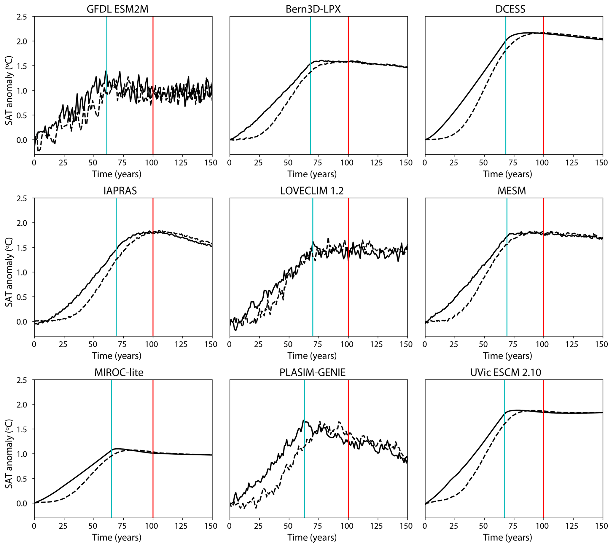
Figure 4Temperature evolution of A1 (1 % to 1000 PgC) and B1 (bell-shaped emissions of 1000 PgC over 100 years) experiments relative to pre-industrial temperature. Solid lines are the A1 experiment and dashed lines are the B1 experiment. The vertical blue line shows when emissions cease in the A1 experiment, and the vertical red line shows where emissions cease in the B1 experiment.
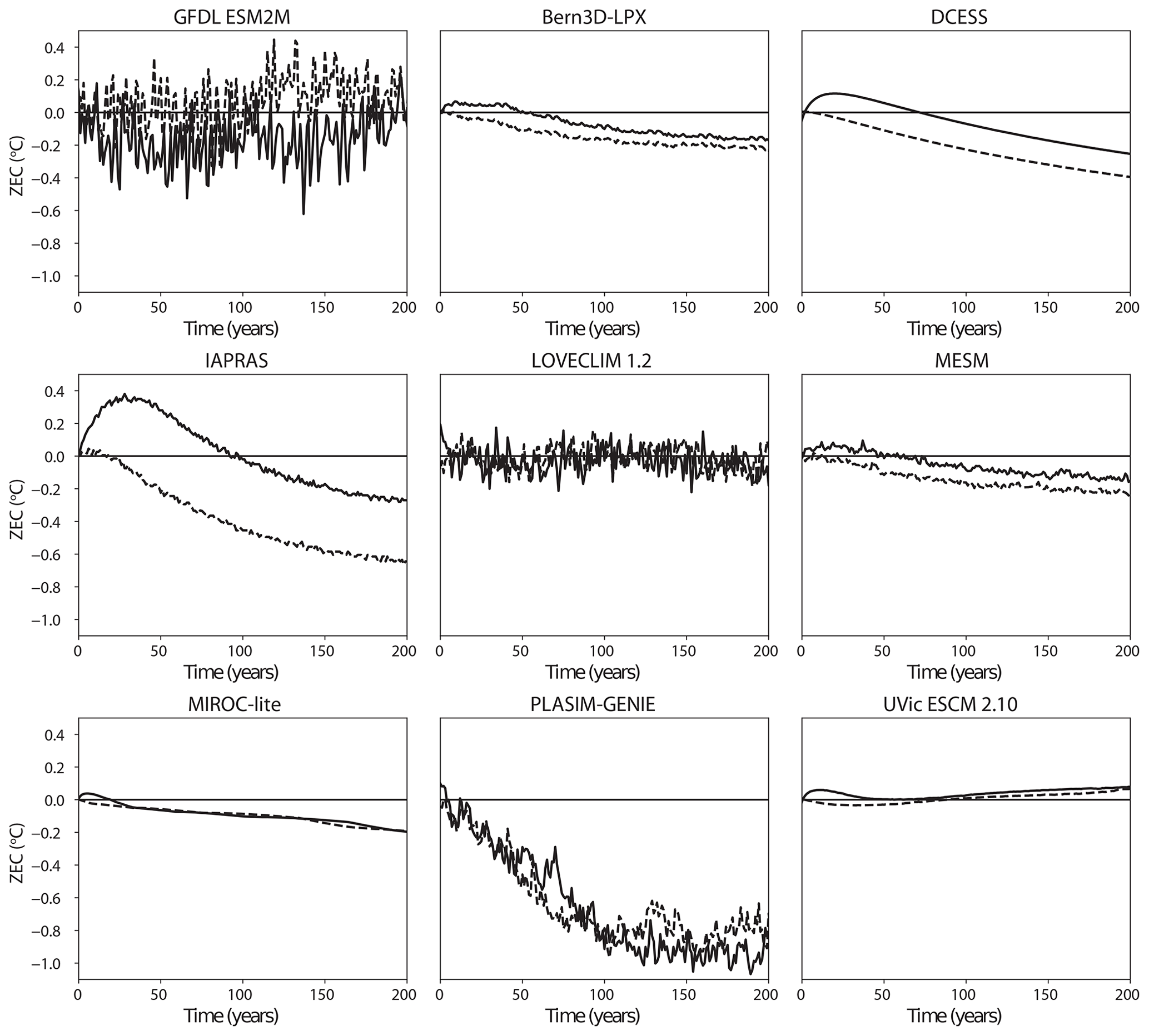
Figure 5ZEC for the A1 (1 % to 1000 PgC) and B1 (bell-shaped emissions of 1000 PgC over 100 years) experiments. The solid lines are the A1 experiment, and the dashed lines are the B1 experiment.
3.3 Sensitivity of ZEC to cumulative emissions
A total of 12 models conducted at least two type A (1 %) experiments, such that ZEC could be calculated for 750, 1000, and 2000 PgC of cumulative emissions, five ESMs (ACCESS, CanESM5, GFDL, MIROC-ES2L, and UKESM), and all of the EMICs except CLIMBER. Two of the models conducted only two of the type A experiments: CanESM5 conducted the A1 and A3 experiments, while LOVECLIM conducted the A1 and A2 experiments. Figure 6 shows the ZEC50 for each model for the three experiments. All of the full ESMs exhibit higher ZEC50 with higher cumulative emissions. The EMICs have a more mixed response with Bern, MESM, LOVECLIM, and UVic showing increased ZEC50 with higher cumulative emissions; DCESS and IAPRAS showing slightly declining ZEC50 with higher cumulative emissions; and P. GENIE showing a strongly declining ZEC50 with higher emissions. The inter-model range for the ZEC50 of the A2 (750 PgC) experiment is −0.31 to 0.30 ∘C, with a mean value of −0.03 ∘C, a median of −0.06 ∘C, and a standard deviation of 0.15 ∘C. The inter-model range of the A3 (2000 PgC) experiment −0.40 to 0.52 ∘C, with a mean of 0.10 ∘C, a median of 0.10 ∘C, and a standard deviation of 0.26 ∘C. Note that different subsets of models conducted each experiment, such that ranges between experiments are not fully comparable.
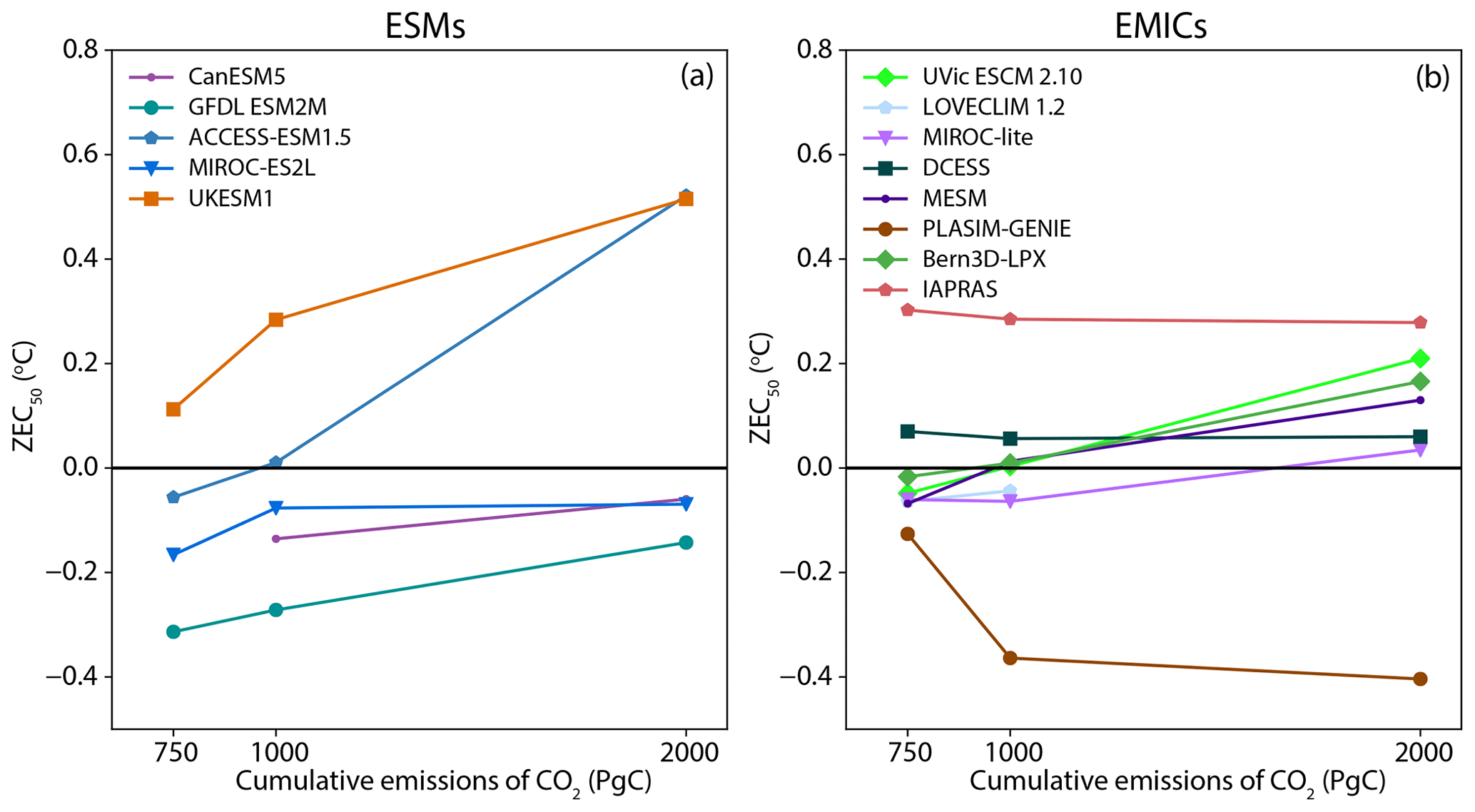
Figure 6Values of ZEC50 for the 750, 1000, and 2000 PgC experiments branching from the 1 % experiment (type A). Panel (a) shows results for full ESMs, and panel(b) shows results for EMICs.
3.4 Analysis of results
The framework introduced in Sect. 2.4 was applied to the ZECMIP output to partition the energy balance components of ZEC into contributions from the warming effect of the reduction in ocean heat uptake (−ΔN) and the effect of the change in radiative forcing from the ocean (Focean) and terrestrial carbon fluxes (Fland). Figure 7 shows the results of this analysis for each model averaged over the period 40 to 59 years after emissions cease for the 1000 PgC 1 % (A1) experiment (the same time interval as ZEC50). The components of the bars in Fig. 7a are the terms of the right-hand side of Eq. (4). The results suggest that both ocean carbon uptake and terrestrial carbon uptake are critical for determining the sign of ZEC in the decades following cessation of emissions. Previous efforts to examine ZEC, while acknowledging the terrestrial carbon sink, have emphasized the role of ocean heat and carbon uptake (Ehlert and Zickfeld, 2017; Williams et al., 2017). These studies also focused on ZEC on timescales of centuries, not decades. In CanESM5 and CNRM the terrestrial carbon sink dominates the reduction in radiative forcing, while in ACCESS, IAPRAS, MESM, P. GENIE, and UVic the ocean carbon uptake dominates the reduction in radiative forcing. The remaining models have substantial contributions from both carbon sinks. In all models the reduction in forcing from ocean carbon uptake is smaller than the reduction in ocean heat uptake, suggesting that the post-cessation net land carbon sink is critical to determining ZEC values. The ocean carbon uptake itself varies substantially between models, with some of the EMICs (P. GENIE, MESM, and IAPRAS) having very high ocean carbon uptake, and two of the ESMs (CanESM5 and CNRM) having very low ocean carbon uptake. Given that the behaviour of the terrestrial carbon cycle varies strongly between models (Friedlingstein et al., 2006; Arora et al., 2013, 2019) and that many models lack feedbacks related to nutrient limitation and permafrost carbon pools, the strong dependence of ZEC50 on terrestrial carbon uptake is concerning for the robustness of ZEC50 estimates. Notably, the three ESMs with the weakest terrestrial carbon sink response (ACCESS, MIROC-ES2L, and UKESM) include terrestrial nutrient limitations (Table A1). However, despite including terrestrial nutrient limitation, Bern and MPI-ESM simulate a terrestrial carbon uptake in the middle and upper parts of the inter-model range, respectively. The UVic model includes permafrost carbon and has a relatively weak terrestrial carbon uptake (Table A2). IAPRAS does not account for either nutrient limitations or permafrost carbon and has the weakest terrestrial carbon uptake among all models studied here (Table A2).
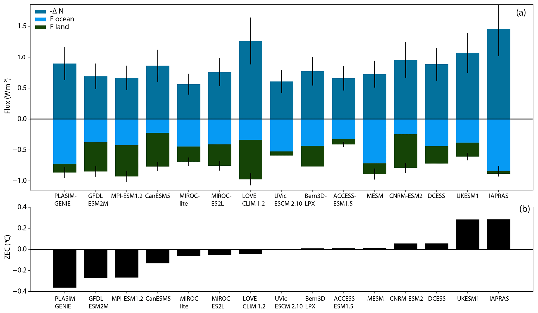
Figure 7(a) Energy fluxes following cessation of CO2 emissions for the 1000 PgC 1 % (A1) experiment. ΔN is the change in ocean heat uptake relative to the time that emissions ceased. A reduction in ocean heat uptake will cause climate warming, hence −ΔN is displayed. Focean is the change in radiative forcing caused by ocean carbon uptake, and Fland is the change in radiative forcing caused by terrestrial carbon uptake. Vertical black lines are estimated uncertainty ranges. (b) ZEC50 values for each model. Models are arranged in ascending order of ZEC50
To further investigate the effect of nutrient limitation on ZEC, we have compared models with and without terrestrial nutrient limitations. Eight of the models that participated in ZECMIP included a representation of the terrestrial nitrogen cycle: ACCESS, CESM2, MIROC-ES2L, MPI-ESM, NorESM, UKESM, Bern, and MESM. One model (ACCESS) includes a representation of the terrestrial phosphorous cycle. Figure 8 shows behaviour of the terrestrial carbon cycle before and after emissions cease for models with and without terrestrial nutrient limitations. Figure 8a shows that consistent with Arora et al. (2019) models with a terrestrial nitrogen cycle on average have a lower carbon uptake than those without. However, after emissions cease there is little difference in the terrestrial uptake of carbon between models with and without nutrient limitations. For both sets of model the median uptake is almost the same at 68 and 63 PgC, respectively, and the range for models without nutrient limitation fully envelops the range for those with nutrient limitations. Thus, while nutrient limitations do not appear to have a controlling influence on the magnitude of the post-cessation terrestrial carbon uptake, they have a marked impact on its uncertainty. As with carbon cycle feedbacks (Arora et al., 2019) those models including terrestrial nitrogen limitation exhibit substantially smaller spread than those which do not. This offers hope for future reductions in ZEC uncertainty as more models begin to include nitrogen (and thereafter phosphorus) limitations on the land carbon sink.
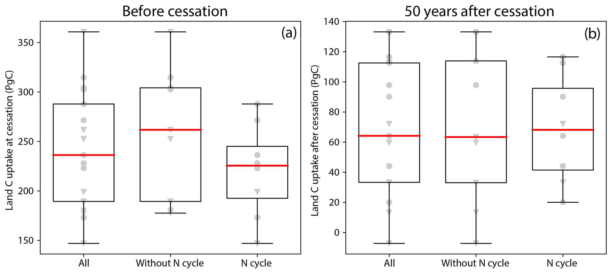
Figure 8Terrestrial carbon uptake for models with and without a nitrogen cycle, before emissions cease and after emissions cease. A total of 8 models have a representation of nutrient limitations while 10 do not. Circles indicate data points for ESMs, and triangles indicate data points for EMICs.
Figure 9a shows the relationship between ocean heat uptake (Fig. 9b), cumulative ocean carbon uptake (Fig. 9c), and the cumulative terrestrial carbon uptake when emissions cease and 50 years after emissions cease. Excluding the clear outlier of IAPRAS, Fig. 9 shows a clear negative relationship () between ocean heat uptake before emissions cease and the change in ocean heat uptake 50 years after emissions cease in the A1 experiment. Thus, models with high ocean uptake before emissions cease tend to have a strong reduction in ocean heat uptake after emissions cease. Similarly, there is a strong (R=0.88) positive relationship between ocean carbon uptake before emissions cease and uptake in the 50 years after emissions cease. The relationship between uptake (or in one case net release) of carbon by the terrestrial biosphere before and after emissions cease is weaker (R=0.72) but clear. Therefore, explaining why the energy balance components illustrated by Fig. 7 vary between models would seem to relate strongly to why models have varying ocean heat, ocean carbon uptake, and terrestrial carbon cycle behaviour before emissions cease.
It has long been suggested that the reason that long-term ZEC was close to zero is compensation between ocean heat and ocean carbon uptake (Matthews and Caldeira, 2008; Solomon et al., 2009; Frölicher and Paynter, 2015), which are both dominated by the ventilation of the thermocline (Sabine et al., 2004; Banks and Gregory, 2006; Xie and Vallis, 2012; Frölicher et al., 2015; Goodwin et al., 2015; Zanna et al., 2019). However, Fig. 7 shows that this generalization is not true for decadal timescales. The two quantities do compensate for one another, but in general the effect from reduction in ocean heat uptake is larger than the change in radiative forcing from the continued ocean carbon uptake. Thus, going forward additional emphasis should be placed on examining the role of the terrestrial carbon sink in ZEC for policy relevant timescales. Also notable is the large uncertainty in effective ocean heat uptake, which originates from the uncertainty in efficacy. As efficacy is related to spatial patterns in ocean heat uptake and coupled shortwave cloud feedbacks (Rose et al., 2014; Andrews et al., 2015) shifts in these patterns in time likely affect the values of ZEC and represent an important avenue for further investigation.
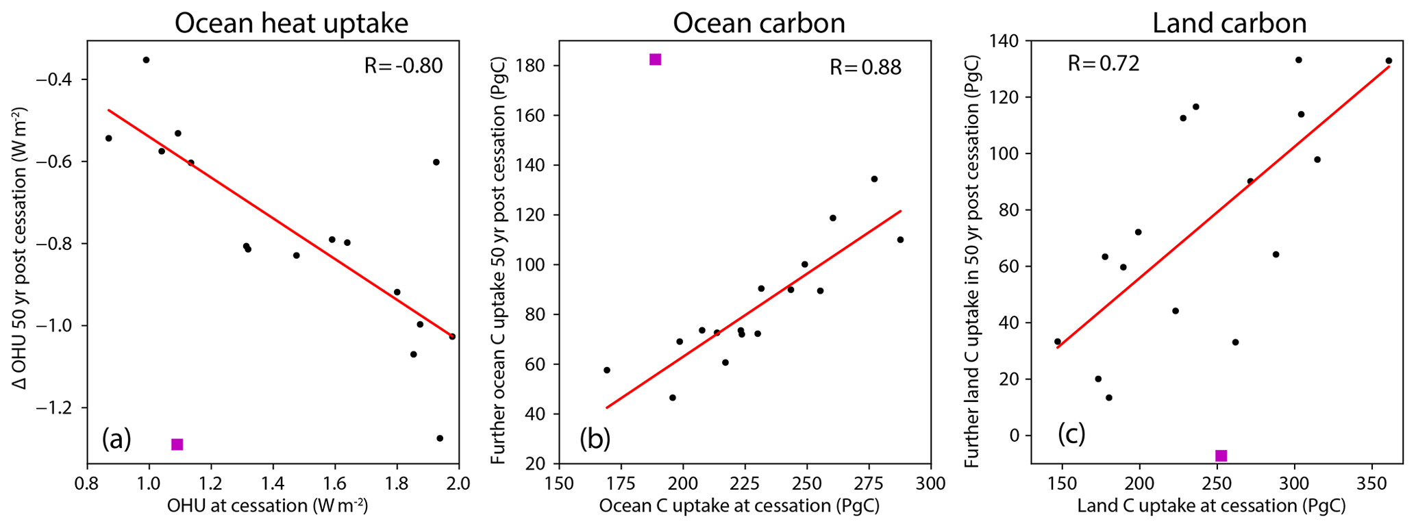
Figure 9Relationship between variables before emissions cease and 50 years after emissions cease. (a) Ocean heat uptake (OHU) is computed for 20-year windows with the value at cessation taken from the 1pctCO2 experiment in a way analogous to the how temperature of cessation is computed. (b) Cumulative ocean carbon uptake and (c) Cumulative land carbon uptake are shown. Each marker represents a value from a single model. The line of best fit excludes the outlier model IAPRAS, which is marked with a magenta square.
Figure 10 compares the energy fluxes for the 10 models that conducted all of the type A (1 %) experiments. All three energy balance components seem to be affected by the cumulative emissions leading up to cessation of emissions; however, there is no universal pattern. Most models show a larger reduction in ocean heat uptake with higher cumulative emissions, but UKESM has the largest reduction for the 1000 PgC experiment. Variations in the reduction in radiative forcing from ocean carbon uptake tend to be small between simulations within each model but show no consistent patterns between models. Most of the models show a smaller terrestrial carbon sink for the 2000 PgC experiment than the other two experiments, the exception being IAPRAS, which shows the opposite pattern. Examining in detail why these factors change in each model could be a productive avenue for future research.
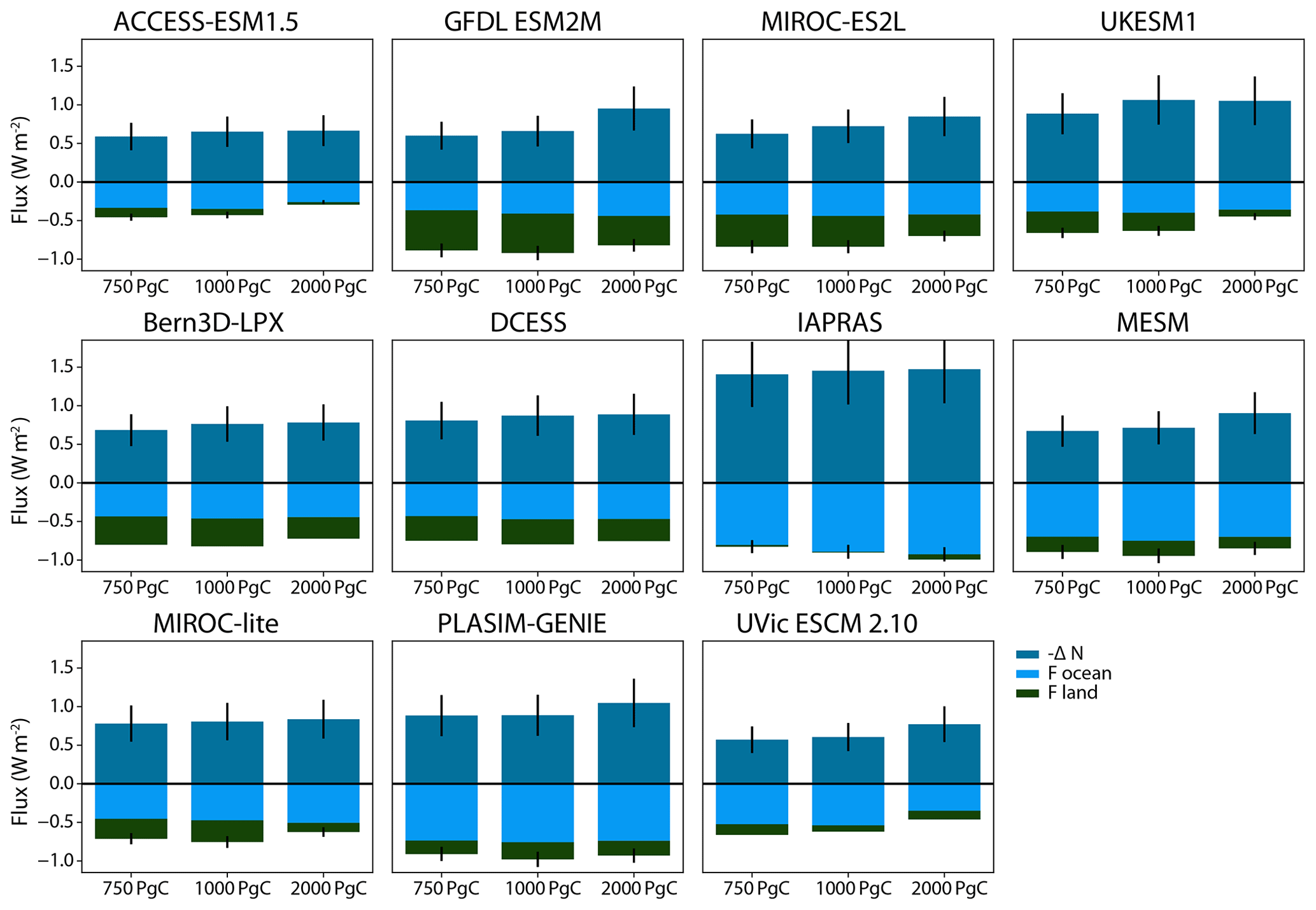
Figure 10Energy fluxes following cessation of CO2 emissions for the type A experiments (1 %) for each model. ΔN is the change in ocean heat uptake relative to the time that emissions ceased. A reduction in ocean heat uptake will cause climate warming, hence −ΔN is displayed. Focean is the change in radiative forcing caused by ocean carbon uptake, and Fland is the change in radiative forcing caused by terrestrial carbon uptake. All fluxes are computed for averages from 40 to 59 years after emissions cease.
3.5 Relationship to other climate metrics
Figure 11 shows the relationship between ECS, TCR, TCRE, realized warming, and ZEC50 for the A1 (1000 PgC) experiment. Realized warming is the ratio of TCR to ECS. TCR is transient warming when CO2 is doubled and ECS is warming at equilibrium following doubling of CO2, their ratio is the fraction of warming from CO2 that has been realized, hence “realized warming” (e.g. Frölicher et al., 2014). ECS shows virtually no correlation with ZEC50 (R=0.04), and thus ZEC and ECS appear to be independent. Both TCR and realized warming show weak positive correlations with ZEC50 (R=0.25 and 0.30, respectively). TCRE shows the strongest relationship to ZEC50 with a correlation coefficient of 0.34. However, these relationships may not be robust due to the small number of non-independent models. The poor correlation between ZEC and other climate metrics is not unexpected as ZEC is determined by the difference in warming caused by reduction in ocean heat uptake and cooling caused by continued land and ocean carbon uptake after the cessation of emissions. Small differences between large quantities are not expected to correlated well to the quantities used to calculate them.
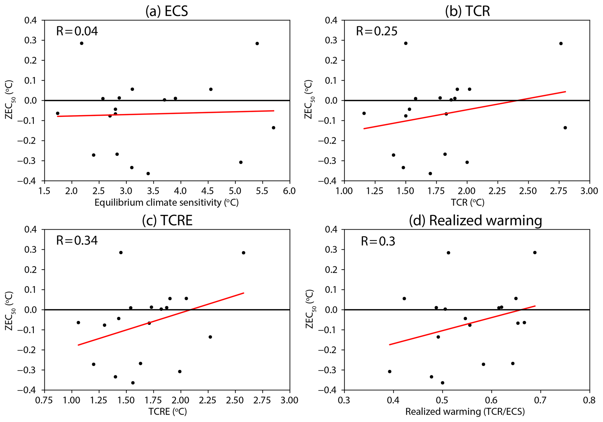
Figure 11Relationship between ECS (a), TCR (b), TCRE (c), realized warming, and (d) ZEC50. The line of best fit is shown in red. Correlation coefficients are displayed in each panel.
Bern and UVic both conducted the ZECMIP experiments with three versions of their models with different equilibrium climate sensitivities, allowing for examination of the effect of ECS on ZEC. Figure 12 shows the ZEC50 for these simulations and shows that for both Bern and UVic higher ECS corresponds to higher ZEC. For Bern for the A1 (1 % 1000 PgC) experiment ZEC50 is 0.01, 0.03, and 0.18 ∘C for ECSs of 2.0, 3.0, and 5.0 ∘C, respectively. For UVic for the A1 (1 % 1000 PgC) experiment ZEC50 is −0.15, 0.01, and 0.22 for ECSs of 2.0, 3.8, and 5.0 ∘C, respectively. Note that the ECS values given here are for true equilibrium climate sensitivity, not effective climate sensitivities as used in the remainder of this study. Figure 13 compares the energy fluxes for the three versions of Bern and UVic. For Bern, ocean carbon uptake is unaffected by climate sensitivity, while for UVic there is a small decline in ocean carbon uptake for an ECS of 5.0 ∘C. For Bern the reduction in ocean heat uptake is larger at higher climate sensitivity, while for UVic this quantity is almost the same for ECSs of 3.8 and 5.0 ∘C. In Bern the terrestrial carbon sink is weaker in versions with higher climate sensitivity. In UVic the terrestrial carbon sink is weakest for a climate sensitivity of 3.8 ∘C. Overall the results suggest a relationship between higher ECS and higher ZEC within these models.

Figure 12Values of 50-year ZEC for the 750, 1000, and 2000 PgC experiments branching from the type A (1 %) for versions of Bern and UVic with varying equilibrium climate sensitivity. Note that the ECS values given here are for true equilibrium climate sensitivity and not effective climate sensitivities as used in the remainder of the study.
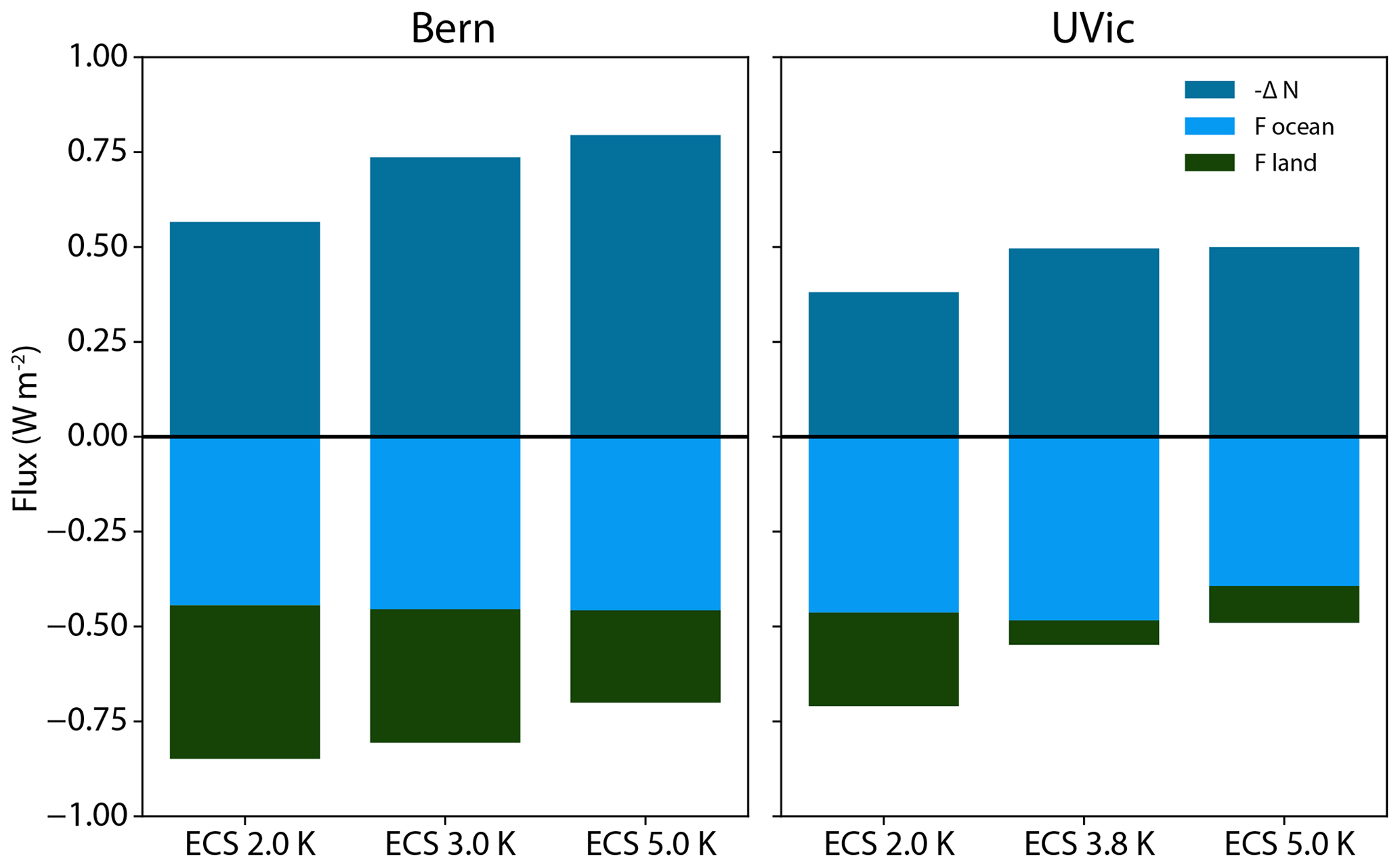
Figure 13Energy fluxes following cessation of CO2 emissions for the type A experiments (1 %) for versions of Bern and UVic with varying equilibrium climate sensitivity. ΔN is the change in ocean heat uptake relative to the time that emissions ceased. A reduction in ocean heat uptake will cause climate warming, hence −ΔN is displayed. Focean is the change in radiative forcing caused by ocean carbon uptake, and Fland is the change in radiative forcing caused by terrestrial carbon uptake. All fluxes computed by averaging from 40 to 59 years after emissions cease.
4.1 Drivers of ZEC
The analysis here has shown that across models decadal-scale ZEC is poorly correlated to other metrics of climate warming, such as TCR and ECS, though relationships may exist within model frameworks (Fig. 12). However, the three factors that drive ZEC, ocean heat uptake, ocean carbon uptake, and net land carbon flux correlate relatively well to their states before emissions cease. Thus, it may be useful to conceptualize ZEC as a function of these three components each evolving in their own way in reaction to the cessation of emissions. Ocean heat uptake evolves due to changes in ocean dynamics (e.g. Frölicher et al., 2015) as well as the complex feedbacks that give rise to changes in ocean heat uptake efficacy (Winton et al., 2010). Ocean carbon uptake evolution is affected by ocean dynamics, changes to ocean biogeochemistry, and changes in atmosphere–ocean CO2 chemical disequilibrium, where the latter is also influenced by land carbon fluxes (e.g. Sarmiento and Gruber, 2006). The response of the land biosphere to cessation of emissions is expected to be complex with contributions from the response of photosynthesis to declining atmospheric CO2 concentration, a continuation of enhanced soil respiration (e.g. Jenkinson et al., 1991), and release of carbon from permafrost soils (Schuur et al., 2015), among other factors. Investigating the evolution of the three components in detail may be a valuable avenue of future analysis. Similarly, given their clearer relationships to the state of the Earth system before emissions cease, focusing on the three components independently may prove useful for building a framework to place emergent constraints on ZEC. Future work will explore evaluation opportunities by assessing relationships between these quantities in the idealized 1 % simulation and values at the end of the historical simulations up to present day.
Our analysis has suggested that the efficacy of ocean heat uptake is crucial for determining the temperature effect from ocean heat uptake following cessation of emissions. Efficacy itself is generated by spatial patterns in ocean heat uptake and shortwave cloud feedback processes (Rose et al., 2014; Andrews et al., 2015). Thus, evaluating how these processes and feedbacks evolve after emissions cease is crucial for better understanding ZEC. As the spatially resolved outputs for ZECMIP are now available (see Data availability at the end of the paper), evaluating such feedbacks presents a promising avenue for future research.
4.2 Policy implications
One of the main motivations to explore ZEC are its implications for policy and society's ability to limit global warming to acceptable levels. Climate policy is currently aiming at limiting global mean temperature increase to well below 2 ∘C and pursuing to limit it to 1.5 ∘C (United Nations, 2015). To stay within these temperature limits, emission reduction targets are being put forward. These targets can take the form of emissions reductions in specific years, like the nationally determined Paris Agreement contributions for the years 2025 or 2030 (Rogelj et al., 2016) but also of net zero emissions targets that cap the cumulative CO2 emissions a country is contributing to the atmosphere (Haites et al., 2013; Rogelj et al., 2015; Geden, 2016). Because ZEC does affect the required stringency of emissions reductions or of the maximum warming one can expect, it is important to clearly understand its implications within a wider policy context. First, for policy analysts and scientists, the quantification of ZEC50 will help inform better estimates of the remaining carbon budget compatible with limiting warming to 1.5 ∘C or well below 2 ∘C over the course of this century. Analysts need to be clear, however, that ZEC50 is only then an adequate adjustment for TCRE-based carbon budget estimates if the TCRE values are based on 1 % CO2 increase simulations. In contrast, however, our results also show that when CO2 emissions ramp down gradually (see the B series of ZECMIP experiments), ZEC50 is generally much smaller because part of it is already realized during the emissions ramp down. Hence, this means that in a situation in which society successfully gradually reduces its global CO2 emissions to net zero at rates comparable to the B2 experiment (see Sect. 3.2), the expected additional warming on timescales of decades to a maximum of a century is small. Finally, over multiple centuries, warming might still further increase or decrease. In the former case, a certain level of carbon dioxide removal would be required over the coming centuries. The level implied by the long-term ZEC, however, represents much less a challenge than the urgent drastic emissions cuts required to limit warming to either 1.5 or 2 ∘C over the next decades (Rogelj et al., 2019b).
4.3 Moving towards ZECMIP-II
For the first iteration of ZECMIP, the experimental protocol has focused solely on the response of the Earth system to zero emissions of CO2. However, many other non-CO2 greenhouse gases, aerosols, and land use changes affect global climate (e.g. IPCC, 2013). To truly explore the question whether global temperature will continue to increase following complete cessation of greenhouse gas and aerosol emissions, the effect of each anthropogenic forcing agent must be accounted for (e.g. Frölicher and Joos, 2010; Matthews and Zickfeld, 2012; Mauritsen and Pincus, 2017; Allen et al., 2018; Smith et al., 2019). We envision a second iteration of ZECMIP accounting for these effects with a set of self-consistent idealized experiments, as a part of the formal CMIP7 process.
Here we have analysed model output from the 18 models that participated in ZECMIP. We have found that the inter-model range of ZEC 50 years after emissions cease for the A1 (1 % to 1000 PgC) experiment is −0.36 to 0.29 ∘C, with a model ensemble mean of −0.07 ∘C, median of −0.05 ∘C, and standard deviation of 0.19 ∘C. Models show a range of temperature evolution after emissions cease from continued warming for centuries to substantial cooling. All models agree that, following cessation of CO2 emissions, the atmospheric CO2 concentration will decline. Comparison between experiments with a sudden cessation of emissions and a gradual reduction in emissions show that long-term temperature change is independent of the pathway of emissions. However, in experiments with a gradual reduction in emissions, a mixture of TCRE and ZEC effects occur as the rate of emissions declines. As the rate of emission reduction in these idealized experiments is similar to that in stringent mitigation scenarios, a similar pattern may emerge if deep emission cuts commence.
ESM simulations agree that higher cumulative emissions lead to a higher ZEC, though some EMICs show the opposite relationship. Analysis of the model output shows that both ocean carbon uptake and the terrestrial carbon uptake are critical for reducing atmospheric CO2 concentration following the cessation of CO2, thus counteracting the warming effect of reduction in ocean heat uptake. The three factors that contribute to ZEC (ocean heat uptake, ocean carbon uptake and net land carbon flux) correlate well to their states prior to the cessation of emissions.
The results of the ZECMIP experiments are broadly consistent with previous work on ZEC, with a most likely value of ZEC that is close to zero and a range of possible model behaviours after emissions cease. In our analysis of ZEC we have shown that terrestrial uptake of carbon plays a more important role in determining that value of ZEC on decadal timescales than has been previously suggested. However, our analysis is consistent with previous results from Ehlert and Zickfeld (2017) and Williams et al. (2017) in terms of ZEC arising from balance of physical and biogeochemical factors.
Overall, the most likely value of ZEC on decadal timescales is assessed to be close to zero, consistent with prior work. However, substantial continued warming for decades or centuries following cessation of emissions is a feature of a minority of the assessed models and thus cannot be ruled out purely on the basis of models.
Table A1Model descriptions of the atmospheric, oceanic, and carbon cycle components for the full Earth System Models (ESMs) that participated in this study.
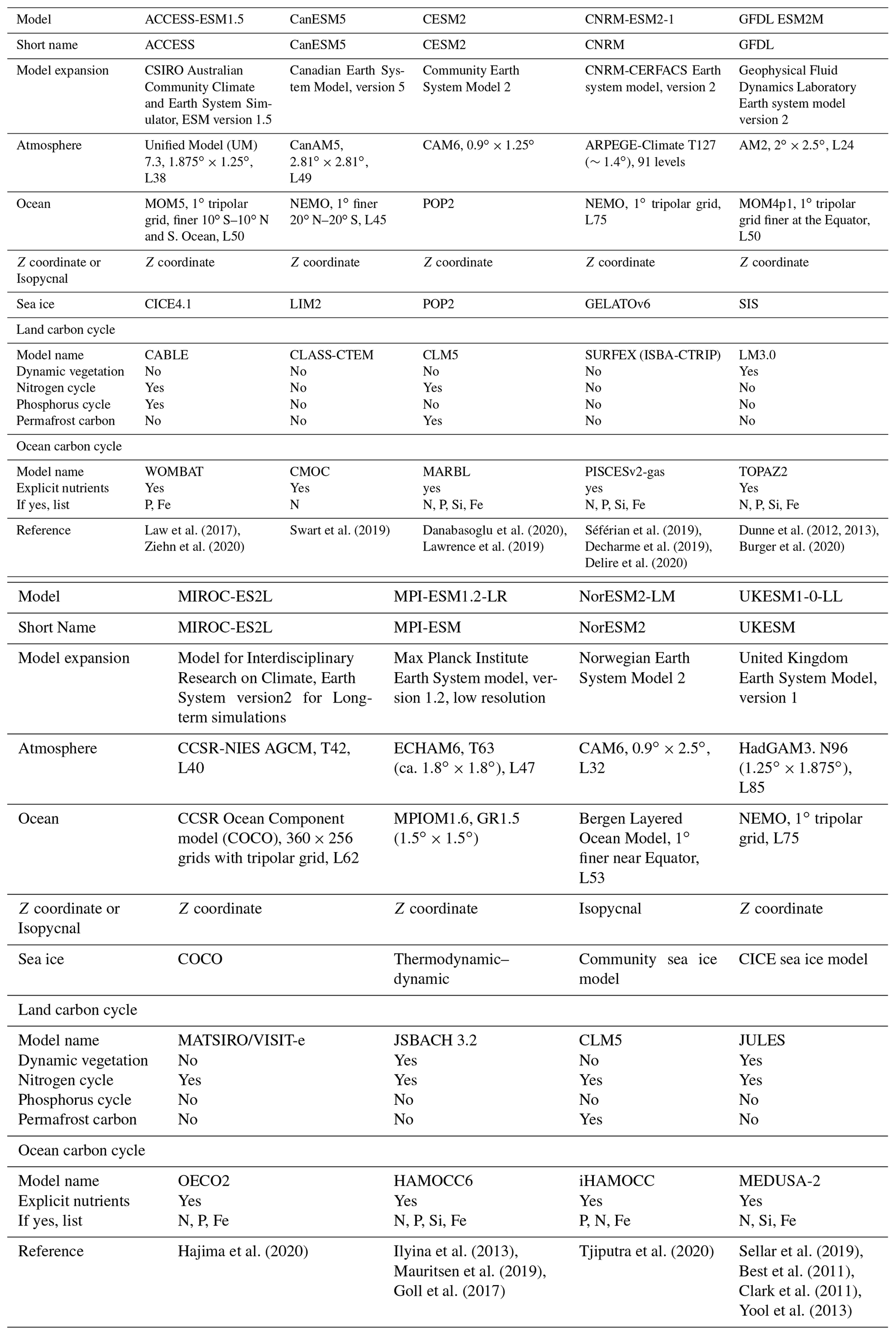
Table A2Model descriptions of the atmospheric, oceanic, and carbon cycle components for Earth system models of intermediate complexity (EMICs) that participated in this study.
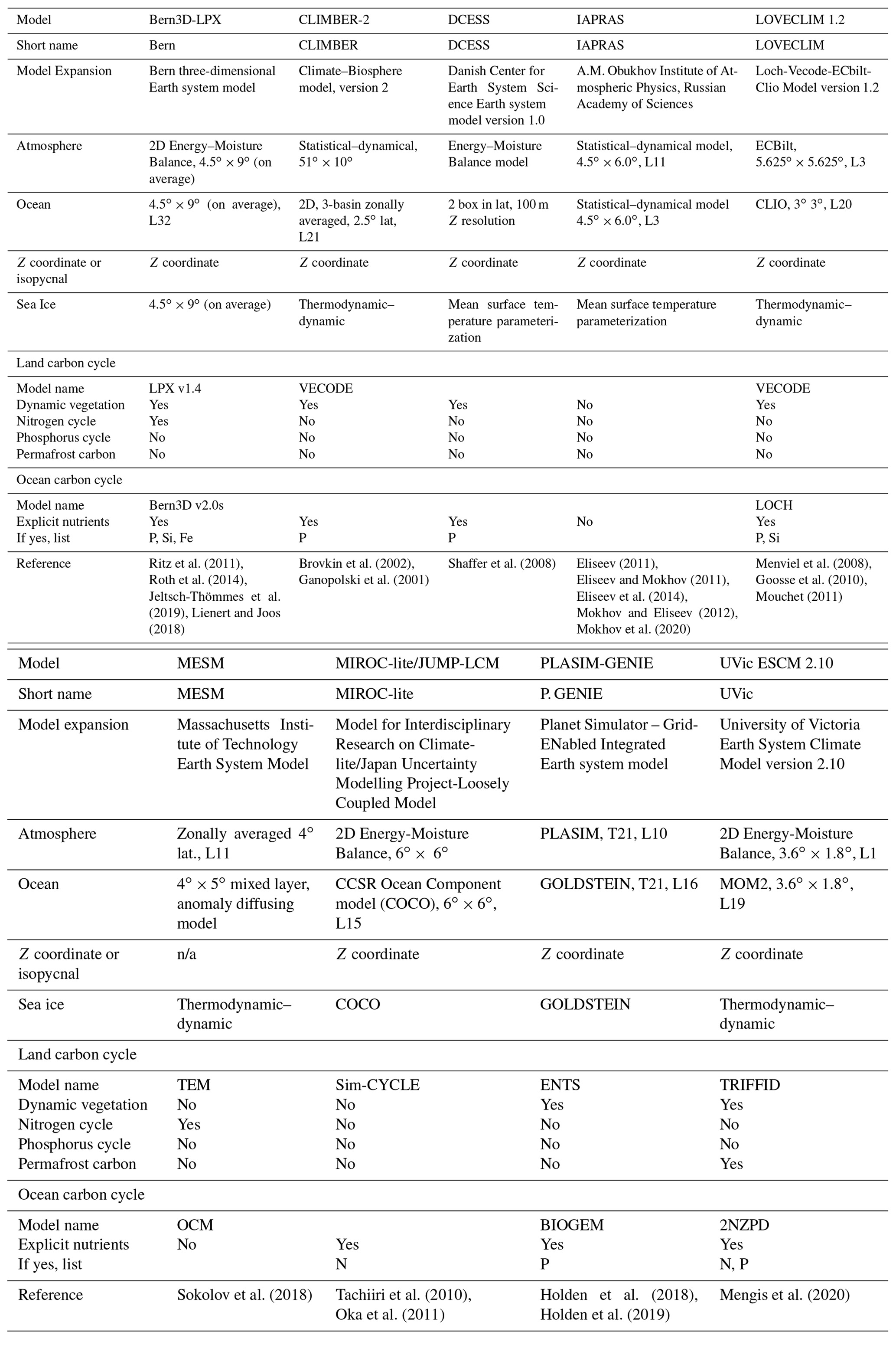
n/a – not applicable.
A key question for this study is explaining why some models have positive ZECs and some models have negative or close to zero ZECs. From elementary theory we understand that the sign of ZEC will depend on the pathway of atmospheric CO2 concentration and ocean heat uptake following cessation of emissions. Complicating this dynamic is that atmospheric CO2 change has contributions both from ocean carbon uptake and the net flux from the terrestrial biosphere. Here we devise a simple method for partitioning the contribution to ZEC from the ocean carbon flux, net land carbon flux, and the ocean heat uptake.
We begin with the forcing response equation (Wigley and Schlesinger, 1985):
where F (W m−2) is radiative forcing, N (W m−2) is planetary heat uptake, ϵ (dimensionless) is the efficacy of planetary heat uptake, λ (W m−2 K−1) is the climate feedback parameter, and T (K) is the change in global temperature (relative to pre-industrial). This equation can be re-written as follows:
To compute the rate of change of temperature we take the derivative of Eq. (B2) in time giving the following equation:
Radiative forcing from CO2 can be approximated using the classical logarithmic relationship (Myhre et al., 1998):
where R (W m−2) is the radiative forcing from an e-fold increase in atmospheric CO2 concentration, CA (PgC) is atmospheric CO2 burden, and CAo (PgC) is the original atmospheric CO2 burden. Recalling the derivative of , the derivative of Eq. (B4) is as follows:
which simplifies to
After emissions cease atmospheric CO2 concentration can be expressed as follows:
where Cze (PgC) is atmospheric CO2 burden at the time emissions reach zero, CO (PgC) is the carbon content of the ocean, and CL (PgC) is the carbon content of land. COze (PgC) is the carbon content of the ocean at the time emissions reach zero and CLze (PgC) is the carbon content of land when emissions reach zero. Thus, the derivative of CA is as follows:
where is the flux of carbon into the ocean fO, and is the flux of carbon into land fL.
Substituting Eq. (B9) in Eq. (B6) we find:
which can be split into
which can be substituted into Eq. (B3):
If we integrate Eq. (B12) from time emissions that reach zero, we get the following equation:
where TZEC (K) is ZEC, Nze (W m−2) is the planetary heat uptake when emissions cease.The integrals and can be computed numerically from ZECMIP output. Therefore, we define the following terms:
and
and thus
Table C1Temperature anomaly relative to the year that emissions ceased, averaged over a 20-year time window centred on the 25th, 50th, and 90th year following the cessation of anthropogenic CO2 emissions (ZEC25, ZEC50, and ZEC90, respectively) for the A2 (750 PgC 1 %) experiment.

Table C2Temperature anomaly relative to the year that emissions ceased averaged over a 20-year time window centred on the 25th, 50th, and 90th year following the cessation of anthropogenic CO2 emissions (ZEC25, ZEC50, and ZEC90, respectively) for the A3 (2000 PgC 1 %) experiment.
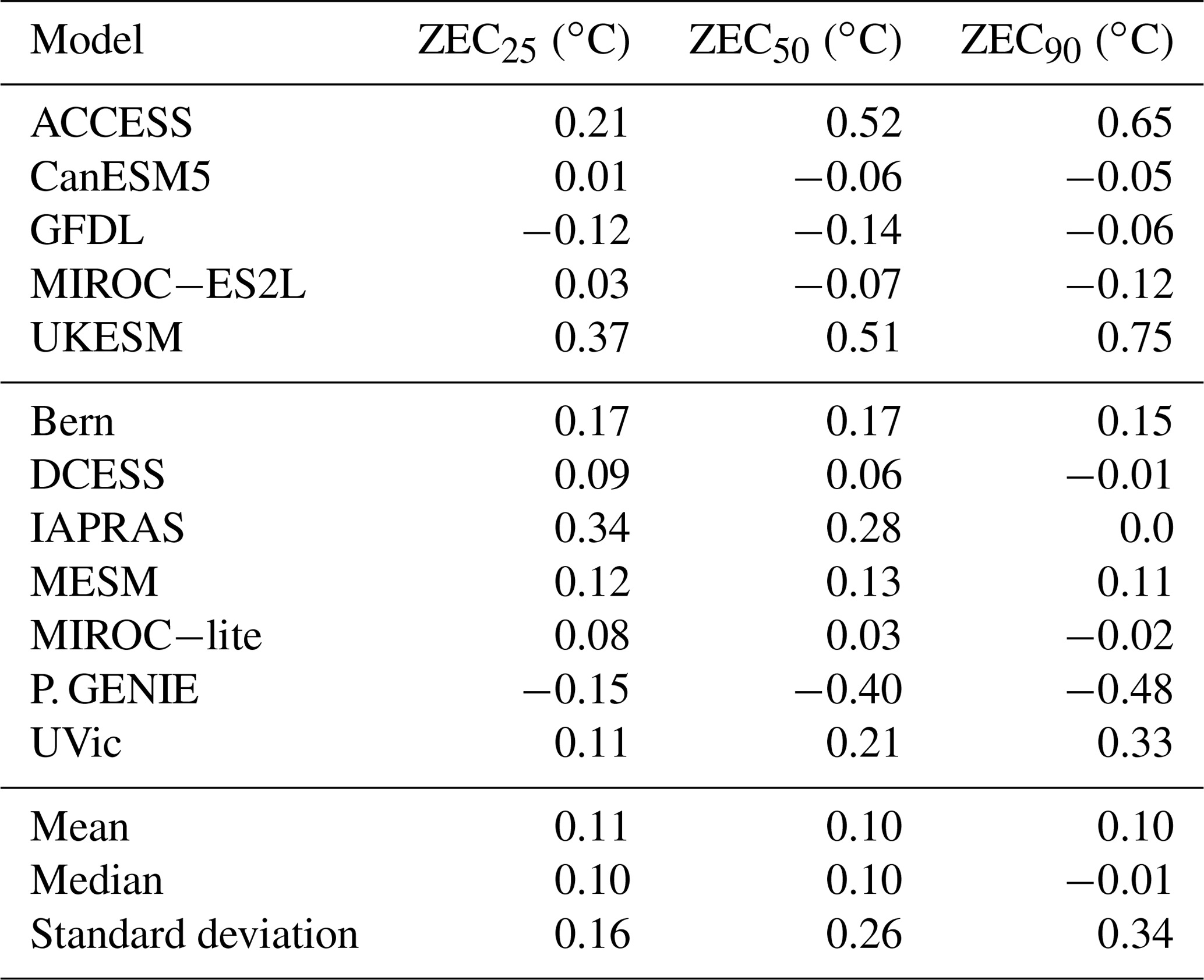
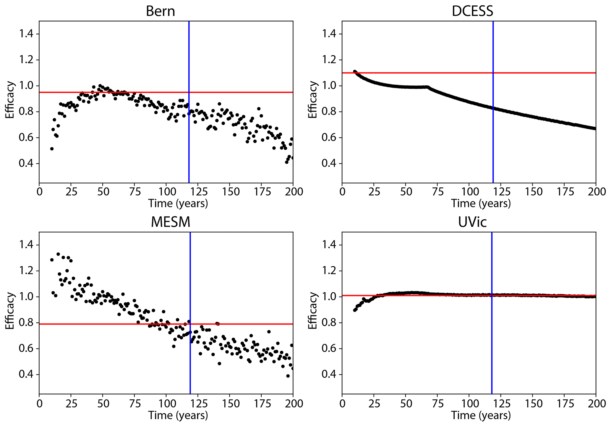
Figure D1Evolution of efficacy for the four EMICs without substantial internal variability. The red horizontal line is the efficacy value estimated from the 1pctCO2 experiment, and the vertical blue line marks 50 years after emissions cease.
ESM data are published and freely available as per CMIP6 data policy on the Earth System Grid Federation (https://esgf-node.llnl.gov/projects/cmip6/, World Climate Research Program, 2020). EMIC data are published and freely available on a dedicated server (http://terra.seos.uvic.ca/ZEC, Eby, 2020). The annual global mean variables used for the present analysis will also be made available on the server.
CDJ, TLF, AHM, JR, HDM, and KZ initiated the research. CDJ and AHM coordinated the project. AHM, VKA, VB, FAB, AVE, TH, PBH, AJT, CK, NM, LM, MM, IIM, RS, GS, JT, JS, TZ, KT, and AO carried out model simulations. AHM, CDJ, TLF, JR, HDM, and KZ contributed to the analysis. ME and NJB contributed critical technical support and programming. AHM, HDM, VKA, and JR contributed significantly to the writing of the paper.
Alexey V. Eliseev is a member of the journal Editorial Board. All other authors declare no competing interests.
Andrew H. MacDougall, Micheal Eby, H. Damon Matthews, and Kirsten Zickfeld are all grateful for support from the National Science and Engineering Research Council of Canada Discovery Grants program. Thomas L. Frölicher, Friedrich A. Burger, and Aurich Jeltsch-Thömmes acknowledge support from the Swiss National Science Foundation. Thomas L. Frölicher, Friedrich A. Burger, Joeri Rogelj, Roland Séférian, and Martine Michou acknowledge support from the EU Horizon 2020 Research and Innovation Programme. Chris D. Jones, Andrew Wiltshire, Victor Brovkin, Roland Séférian and Martine Michou acknowledge the EU Horizon 2020 CRESCENDO project. Chris D. Jones and Andrew Wiltshire acknowledge the Joint UK BEIS–Defra Met Office Hadley Centre Climate Programme. Alexey V. Eliseev and Igor I. Mokhov were supported by the Russian Foundation for Basic Research. Tomohiro Hajima and Kaoru Tachiiri acknowledge support from “Integrated Research Program for Advancing Climate Models” by the Ministry of Education, Culture, Sports, Science, and Technology of Japan. Philip B. Holden was funded by LC3M, a Leverhulme Trust Research Centre Award. Aurich Jeltsch-Thömmes acknowledges support from the Oeschger Centre for Climate Change Research. Gary Shaffer was supported by FONDECYT. Laurie Menviel acknowledges support from the Australian Research Council. Jerry Tjiputra and Jörg Schwinger acknowledge Research Council of Norway funded projects KeyClim and IMPOSE.
Andrew H. MacDougall is thankful to Compute Canada. GFDL ESM2M simulations were performed at the Swiss National Supercomputing Centre (CSCS). Victor Brovkin is grateful to Thomas Raddatz and Veronika Gayler for their assistance with the MPI-ESM experimental setup. Roland Séférian and Martine Michou acknowledge supercomputing time provided by the Météo-France/DSI supercomputing centre.
The authors thank all participants of the expert workshop on carbon budgets, co-organized with the support of the Global Carbon Project, the CRESCENDO project, the University of Melbourne, and Simon Fraser University, for discussions that initiated the authors' thinking about ZECMIP.
We thank Ric Williams and an anonymous reviewer for their helpful comments.
This research has been supported by the Natural Sciences and Engineering Research Council of Canada, the Swiss National Science Foundation (grant nos. PP00P2-170687, 200020, and 172476), the European Union's Horizon 2020 Research and Innovation Programme (grant nos. 821003, 820829, and 641816), the Joint UK BEIS–Defra Met Office Hadley Centre Climate Programme (grant no. GA01101), the EU Horizon 2020 CRESCENDO (grant no. 641816), the Russian Foundation for Basic Research (grant nos. 18-05-00087 and 19-17-00240), the Integrated Research Program for Advancing Climate Models, the Fondos de Desarrollo de la Astronomía Nacional (grant no. 1190230), the Australian Research Council (grant no. FT180100606), the Leverhulme Trust Research Centre Award (grant no. RC-2015-029), and the Research Council of Norway (grant nos. 295046 and 294930).
This paper was edited by Carolin Löscher and reviewed by Ric Williams and one anonymous referee.
Allen, M. R., Dube, O. P., Solecki, W., Aragón-Durand, F., Cramer, W., Humphreys, S., Kainuma, M., Kala, J., Mahowald, N., Mulugetta, Y., Perez, R., Wairiu, M., and Zickfeld, K.: Framing and Context, in: Global warming of 1.5 ∘C. An IPCC Special Report on the impacts of global warming of 1.5 ∘C above pre-industrial levels and related global greenhouse gas emission pathways, in the context of strengthening the global response to the threat of climate change, sustainable development, and efforts to eradicate poverty, World Meteorological Organization, Cambridge, UK and New York, NY, USA, 2018. a, b, c, d, e
Andrews, T., Gregory, J. M., and Webb, M. J.: The dependence of radiative forcing and feedback on evolving patterns of surface temperature change in climate models, J. Climate, 28, 1630–1648, 2015. a, b, c
Archer, D. and Brovkin, V.: The millennial atmospheric lifetime of anthropogenic CO2, Climatic Change, 90, 283–297, 2008. a
Archer, D., Eby, M., Brovkin, V., Ridgwell, A., Cao, L., Mikolajewicz, U., Caldeira, K., Matsumoto, K., Munhoven, G., Montenegro, A., and Tokos, K.: Atmospheric lifetime of fossil fuel carbon dioxide, Annu. Rev. Earth Pl. Sc., 37, 117–134, 2009. a
Arora, V. K., Boer, G. J., Friedlingstein, P., Eby, M., Jones, C. D., Christian, J. R., Bonan, G., Bopp, L., Brovkin, V., Cadule, P., Ilyina, T. H., Lindsay, K., Tjiputra, J. F., and Wu, T.: Carbon-Concentration and Carbon-Climate Feedbacks in CMIP5 Earth System Models, J. Climate, 26, 5289–5314, 2013. a
Arora, V. K., Katavouta, A., Williams, R. G., Jones, C. D., Brovkin, V., Friedlingstein, P., Schwinger, J., Bopp, L., Boucher, O., Cadule, P., Chamberlain, M. A., Christian, J. R., Delire, C., Fisher, R. A., Hajima, T., Ilyina, T., Joetzjer, E., Kawamiya, M., Koven, C., Krasting, J., Law, R. M., Lawrence, D. M., Lenton, A., Lindsay, K., Pongratz, J., Raddatz, T., Séférian, R., Tachiiri, K., Tjiputra, J. F., Wiltshire, A., Wu, T., and Ziehn, T.: Carbon-concentration and carbon-climate feedbacks in CMIP6 models, and their comparison to CMIP5 models, Biogeosciences Discuss., https://doi.org/10.5194/bg-2019-473, in review, 2019. a, b, c
Banks, H. T. and Gregory, J. M.: Mechanisms of ocean heat uptake in a coupled climate model and the implications for tracer based predictions of ocean heat uptake, Geophys. Res. Lett., 33, L07608, https://doi.org/10.1029/2005GL025352, 2006. a
Best, M. J., Pryor, M., Clark, D. B., Rooney, G. G., Essery, R. L. H., Ménard, C. B., Edwards, J. M., Hendry, M. A., Porson, A., Gedney, N., Mercado, L. M., Sitch, S., Blyth, E., Boucher, O., Cox, P. M., Grimmond, C. S. B., and Harding, R. J.: The Joint UK Land Environment Simulator (JULES), model description – Part 1: Energy and water fluxes, Geosci. Model Dev., 4, 677–699, https://doi.org/10.5194/gmd-4-677-2011, 2011. a
Brovkin, V., Bendtsen, J., Claussen, M., Ganopolski, A., Kubatzki, C., Petoukhov, V., and Andreev, A.: Carbon cycle, vegetation, and climate dynamics in the Holocene: Experiments with the CLIMBER-2 model, Global Biogeochem. Cy., 16, 86–1, 2002. a
Burger, F. A., Frölicher, T. L., and John, J. G.: Increase in ocean acidity variability and extremes under increasing atmospheric CO2, Biogeosciences Discuss., https://doi.org/10.5194/bg-2020-22, in review, 2020. a
Byrne, B. and Goldblatt, C.: Radiative forcing at high concentrations of well-mixed greenhouse gases, Geophys. Res. Lett., 41, 152–160, 2014. a
Cao, L., Eby, M., Ridgwell, A., Caldeira, K., Archer, D., Ishida, A., Joos, F., Matsumoto, K., Mikolajewicz, U., Mouchet, A., Orr, J. C., Plattner, G.-K., Schlitzer, R., Tokos, K., Totterdell, I., Tschumi, T., Yamanaka, Y., and Yool, A.: The role of ocean transport in the uptake of anthropogenic CO2, Biogeosciences, 6, 375–390, https://doi.org/10.5194/bg-6-375-2009, 2009. a
Charney, J., Arakawa, A., Baker, D., Bolin, B., Dickinson, R., Goody, R., Leith, C., Stommel, H., and Wunsch, C.: Carbon dioxide and climate: a scientific assessment: report of an ad hoc study group on carbon dioxide and climate, woods hole, Massachusetts, July 23–27, 1979 to the climate research board, assembly of mathematical and physical sciences, National Research Council, National Academy of Sciences, Climate Research Board, Washington, DC, USA, 1979. a
Clark, D. B., Mercado, L. M., Sitch, S., Jones, C. D., Gedney, N., Best, M. J., Pryor, M., Rooney, G. G., Essery, R. L. H., Blyth, E., Boucher, O., Harding, R. J., Huntingford, C., and Cox, P. M.: The Joint UK Land Environment Simulator (JULES), model description – Part 2: Carbon fluxes and vegetation dynamics, Geosci. Model Dev., 4, 701–722, https://doi.org/10.5194/gmd-4-701-2011, 2011. a
Danabasoglu, G., Lamarque, J.-F., Bacmeister, J., Bailey, D. A., DuVivier, A. K., Edwards, J., Emmons, L. K., Fasullo, J., Garcia, R., Gettelman, A., Hannay, C., Holland, M. M., Large, W. G., Lawrence, D. M., Lenaerts, J. T. M., Lindsay, K., Lipscomb, W. H., Mills, M. J., Neale, R., Oleson, K. W., Otto-Bliesner, B., Phillips, A. S., Sacks, W., Tilmes, S., van Kampenhout, L., Vertenstein, M., Bertini, A., Dennis, J., Deser, C., Fischer, C., Fox-Kemper, B., Kay, J. E., Kinnision, D., Kushner, P. J., Long, M. C., Mickelson, S., Moore, J. K., Nienhouse, E., Polvani, L., Rasch, P. J., and Strand, W. G.: The Community Earth System Model 2 (CESM2), J. Adv. Model. Earth Sy., in review, 2020. a
Davis, S. J. and Socolow, R. H.: Commitment accounting of CO2 emissions, Environ. Res. Lett., 9, 084018, https://doi.org/10.1088/1748-9326/9/8/084018, 2014. a
Davis, S. J., Caldeira, K., and Matthews, H. D.: Future CO2 emissions and climate change from existing energy infrastructure, Science, 329, 1330–1333, 2010. a
Decharme, B., Delire, C., Minvielle, M., Colin, J., Vergnes, J.-P., Alias, A., Saint-Martin, D., Séférian, R., Sénési, S., and Voldoire, A.: Recent Changes in the ISBA-CTRIP Land Surface System for Use in the CNRM-CM6 Climate Model and in Global Off-Line Hydrological Applications, J. Adv. Model. Earth Sy., 11, 1207–1252, https://doi.org/10.1029/2018MS001545, 2019. a
Delire, C., Séférian, R., Decharme, B., Alkama, R., Carrer, D., Joetzjer, E., Morel, X., and Rocher, M.: The global land carbon cycle simulated with ISBA, J. Adv. Model. Earth Sy., https://doi.org/10.1029/2019MS001886, online first, 2020. a
Dunne, J. P., John, J. G., Adcroft, A. J., Griffies, S. M., Hallberg, R. W., Shevliakova, E., Stouffer, R. J., Cooke, W., Dunne, K. A., Harrison, M. J., Krasting, J. P., Malyshev, S. L., Milly, P. C. D., Phillipps, P. J., Sentman, L. T., Samuels, B. L., Spelman, M. J., Winton, M., Wittenberg, A. T., and Zadeh, N.: GFDL's ESM2 global coupled climate-carbon earth system models. Part I: Physical formulation and baseline simulation characteristics, J. Climate, 25, 6646–6665, 2012. a
Dunne, J. P., John, J. G., Shevliakova, E., Stouffer, R. J., Krasting, J. P., Malyshev, S. L., Milly, P., Sentman, L. T., Adcroft, A. J., Cooke, W., Dunne, K. A., Griffies, S. M., Hallberg, R. W., Harrison, M. J., Levy, H., Wittenberg, A. T., Phillips, P. J., and Zadeh, N.: GFDL's ESM2 global coupled climate-carbon earth system models. Part II: carbon system formulation and baseline simulation characteristics, J. Climate, 26, 2247–2267, 2013. a
Eby, M.: Zero Emissions Commitment Model Intercomparison Project, Globally averaged data and EMIC data repository, University of Victoria, available at: http://terra.seos.uvic.ca/ZEC, last access: June 2020. a
Eby, M., Zickfeld, K., Montenegro, A., Archer, D., Meissner, K. J., and Weaver, A. J.: Lifetime of Anthropogenic Climate Change: Millennial Time Scales of Potential CO2 and Surface Temperature Perturbations, J. Climate, 22, 2501–2511, https://doi.org/10.1175/2008JCLI2554.1, 2009. a
Ehlert, D. and Zickfeld, K.: What determines the warming commitment after cessation of CO2 emissions?, Environ. Res. Lett., 12, 015002, https://doi.org/10.1088/1748-9326/aa564a, 2017. a, b, c, d
Eliseev, A.: Estimation of changes in characteristics of the climate and carbon cycle in the 21st century accounting for the uncertainty of terrestrial biota parameter values, Izvestiya, Atmos. Ocean. Phys., 47, 131, https://doi.org/10.1134/S0001433811020046, 2011. a
Eliseev, A. V. and Mokhov, I. I.: Uncertainty of climate response to natural and anthropogenic forcings due to different land use scenarios, Adv. Atmos. Sci., 28, 1215, https://doi.org/10.1007/s00376-010-0054-8, 2011. a
Eliseev, A. V., Mokhov, I. I., and Chernokulsky, A. V.: An ensemble approach to simulate CO2 emissions from natural fires, Biogeosciences, 11, 3205–3223, https://doi.org/10.5194/bg-11-3205-2014, 2014. a
Enting, I. G., Wigley, T., and Heimann, M.: Future emissions and concentrations of carbon dioxide: key ocean/atmosphere/land analyses, CSIRO, Australia, 1994. a
Etminan, M., Myhre, G., Highwood, E., and Shine, K.: Radiative forcing of carbon dioxide, methane, and nitrous oxide: A significant revision of the methane radiative forcing, Geophys. Res. Lett., 43, 12614–12623, 2016. a
Eyring, V., Bony, S., Meehl, G. A., Senior, C. A., Stevens, B., Stouffer, R. J., and Taylor, K. E.: Overview of the Coupled Model Intercomparison Project Phase 6 (CMIP6) experimental design and organization, Geosci. Model Dev., 9, 1937–1958, https://doi.org/10.5194/gmd-9-1937-2016, 2016. a, b, c
Friedlingstein, P., Cox, P., Betts, R., Bopp, L., von Bloh, W., Brovkin, V., Cadule, P., Doney, S., Eby, M., Fung, I., Bala, G., John, J., Jones, C., Joos, F., Kato, T., Kawamiy, M., Knorr, W., Lindsay, K., Matthews, H. D., Raddatz, T., Rayner, P., Reick, C., Roeckner, E., Schnitzler, K. G., Schnur, R., Strassmann, K., Weaver, A. J., Yoshikawa, C., and Zeng, N.: Climate–Carbon Cycle Feedback Analysis: Results from the C4MIP Model Intercomparison, J. Climate, 19, 3337–3353, 2006. a
Frölicher, T. L. and Joos, F.: Reversible and irreversible impacts of greenhouse gas emissions in multi-century projections with the NCAR global coupled carbon cycle-climate model, Clim. Dynam., 35, 1439–1459, 2010. a, b, c, d
Frölicher, T. L. and Paynter, D. J.: Extending the relationship between global warming and cumulative carbon emissions to multi-millennial timescales, Environ. Res. Lett., 10, 075002, https://doi.org/10.1088/1748-9326/10/7/075002, 2015. a, b, c, d, e
Frölicher, T. L., Winton, M., and Sarmiento, J. L.: Continued global warming after CO2 emissions stoppage, Nat. Clim. Change, 4, 40–44, 2014. a, b
Frölicher, T. L., Sarmiento, J. L., Paynter, D. J., Dunne, J. P., Krasting, J. P., and Winton, M.: Dominance of the Southern Ocean in anthropogenic carbon and heat uptake in CMIP5 models, J. Climate, 28, 862–886, 2015. a, b
Ganopolski, A., Petoukhov, V., Rahmstorf, S., Brovkin, V., Claussen, M., Eliseev, A., and Kubatzki, C.: CLIMBER-2: a climate system model of intermediate complexity. Part II: model sensitivity, Clim. Dynam., 17, 735–751, 2001. a
Geden, O.: An actionable climate target, Nat. Geosci., 9, 340, https://doi.org/10.1038/ngeo2699, 2016. a
Gillett, N., Arora, V., Zickfeld, K., Marshall, S., and Merryfield, W.: Ongoing climate change following a complete cessation of carbon dioxide emissions, Nat. Geosci., 4, 83–87, 2011. a, b
Goll, D. S., Winkler, A. J., Raddatz, T., Dong, N., Prentice, I. C., Ciais, P., and Brovkin, V.: Carbon–nitrogen interactions in idealized simulations with JSBACH (version 3.10), Geosci. Model Dev., 10, 2009–2030, https://doi.org/10.5194/gmd-10-2009-2017, 2017. a
Goodwin, P., Williams, R. G., Follows, M. J., and Dutkiewicz, S.: Ocean–atmosphere partitioning of anthropogenic carbon dioxide on centennial timescales, Global Biogeochem. Cy., 21, GB1014, https://doi.org/10.1029/2006GB002810, 2007. a
Goodwin, P., Williams, R. G., and Ridgwell, A.: Sensitivity of climate to cumulative carbon emissions due to compensation of ocean heat and carbon uptake, Nat. Geosci., 8, 29–34, 2015. a
Goosse, H., Brovkin, V., Fichefet, T., Haarsma, R., Huybrechts, P., Jongma, J., Mouchet, A., Selten, F., Barriat, P.-Y., Campin, J.-M., Deleersnijder, E., Driesschaert, E., Goelzer, H., Janssens, I., Loutre, M.-F., Morales Maqueda, M. A., Opsteegh, T., Mathieu, P.-P., Munhoven, G., Pettersson, E. J., Renssen, H., Roche, D. M., Schaeffer, M., Tartinville, B., Timmermann, A., and Weber, S. L.: Description of the Earth system model of intermediate complexity LOVECLIM version 1.2, Geosci. Model Dev., 3, 603–633, https://doi.org/10.5194/gmd-3-603-2010, 2010. a
Gregory, J., Ingram, W., Palmer, M., Jones, G., Stott, P., Thorpe, R., Lowe, J., Johns, T., and Williams, K.: A new method for diagnosing radiative forcing and climate sensitivity, Geophys. Res. Lett., 31, L03205, https://doi.org/10.1029/2003GL018747, 2004. a, b, c
Gregory, J. M., Andrews, T., and Good, P.: The inconstancy of the transient climate response parameter under increasing CO2, Philos. T. R. Soc. A, 373, 20140417, https://doi.org/10.1098/rsta.2014.0417, 2015. a, b
Haites, E., Yamin, F., and Höhne, N.: Possible Elements of a 2015 Legal Agreement on Climate Change, IDDRI SciencesPo Working Paper, 1–24, available at: http://theredddesk.org/sites/default/files/resources/pdf/Possible Elements of a 2015 Legal Agreement on Climate Change.pdf (last access: 10 June 2020), 2013. a
Hajima, T., Watanabe, M., Yamamoto, A., Tatebe, H., Noguchi, M. A., Abe, M., Ohgaito, R., Ito, A., Yamazaki, D., Okajima, H., Ito, A., Takata, K., Ogochi, K., Watanabe, S., and Kawamiya, M.: Development of the MIROC-ES2L Earth system model and the evaluation of biogeochemical processes and feedbacks, Geosci. Model Dev., 13, 2197–2244, https://doi.org/10.5194/gmd-13-2197-2020, 2020. a
Hare, B. and Meinshausen, M.: How much warming are we committed to and how much can be avoided?, Climatic Change, 75, 111–149, 2006. a, b, c
Holden, P. B., Edwards, N. R., Ridgwell, A., Wilkinson, R., Fraedrich, K., Lunkeit, F., Pollitt, H., Mercure, J.-F., Salas, P., Lam, A., Knobloch, F., Chewpreecha, U., and Viñuales, J. E.: Climate–carbon cycle uncertainties and the Paris Agreement, Nat. Clim. Change, 8, 609–613, https://doi.org/10.1038/s41558-018-0197-7, 2018. a
Holden, P. B., Edwards, N. R., Rangel, T. F., Pereira, E. B., Tran, G. T., and Wilkinson, R. D.: PALEO-PGEM v1.0: a statistical emulator of Pliocene–Pleistocene climate, Geosci. Model Dev., 12, 5137–5155, https://doi.org/10.5194/gmd-12-5137-2019, 2019. a
Ilyina, T., Six, K. D., Segschneider, J., Maier-Reimer, E., Li, H., and Núñez-Riboni, I.: Global ocean biogeochemistry model HAMOCC: Model architecture and performance as component of the MPI-Earth system model in different CMIP5 experimental realizations, J. Adv. Model. Earth Sy., 5, 287–315, 2013. a
IPCC: Summary for Policymakers, in: Working Group I Contribution to the Intergovernmental Panel on Climate Change Fifth Assessment Report Climate Change 2013: The Physical Science Basis, edited by: Alexander, L., Allen, S., Bindoff, N. L., Bréon, F.-M., Church, J., Cubasch, U., Emori, S., Forster, P., Friedlingstein, P., Gillett, N., Gregory, J., Hartmann, D., Jansen, E., Kirtman, B., Knutti, R., Kanikicharla, K. K., Lemke, P., Marotzke, J., Masson-Delmotte, V., Meehl, G., Mokhov, I., Piao, S., Plattner, G.-K., Dahe, Q., Ramaswamy, V., Randall, D., Rhein, M., Rojas, M., Sabine, C., Shindell, D., Stocker, T. F., Talley, L., Vaughan, D., and Xie, S.-P., Cambridge University Press, Cambridge, UK and New York, NY, USA, 2013. a
Jeltsch-Thömmes, A., Battaglia, G., Cartapanis, O., Jaccard, S. L., and Joos, F.: Low terrestrial carbon storage at the Last Glacial Maximum: constraints from multi-proxy data, Clim. Past, 15, 849–879, https://doi.org/10.5194/cp-15-849-2019, 2019. a
Jenkinson, D., Adams, D., and Wild, A.: Model estimates of CO2 emissions from soil in response to global warming, Nature, 351, 304–306, 1991. a
Jones, C. D., Frölicher, T. L., Koven, C., MacDougall, A. H., Matthews, H. D., Zickfeld, K., Rogelj, J., Tokarska, K. B., Gillett, N. P., Ilyina, T., Meinshausen, M., Mengis, N., Séférian, R., Eby, M., and Burger, F. A.: The Zero Emissions Commitment Model Intercomparison Project (ZECMIP) contribution to C4MIP: quantifying committed climate changes following zero carbon emissions, Geosci. Model Dev., 12, 4375–4385, https://doi.org/10.5194/gmd-12-4375-2019, 2019. a, b, c, d
Joos, F., Roth, R., Fuglestvedt, J. S., Peters, G. P., Enting, I. G., von Bloh, W., Brovkin, V., Burke, E. J., Eby, M., Edwards, N. R., Friedrich, T., Frölicher, T. L., Halloran, P. R., Holden, P. B., Jones, C., Kleinen, T., Mackenzie, F. T., Matsumoto, K., Meinshausen, M., Plattner, G.-K., Reisinger, A., Segschneider, J., Shaffer, G., Steinacher, M., Strassmann, K., Tanaka, K., Timmermann, A., and Weaver, A. J.: Carbon dioxide and climate impulse response functions for the computation of greenhouse gas metrics: a multi-model analysis, Atmos. Chem. Phys., 13, 2793–2825, https://doi.org/10.5194/acp-13-2793-2013, 2013. a
Knutti, R., Rugenstein, M. A., and Hegerl, G. C.: Beyond equilibrium climate sensitivity, Nat. Geosci., 10, 727–736, https://doi.org/10.1038/ngeo3017, 2017. a
Law, R. M., Ziehn, T., Matear, R. J., Lenton, A., Chamberlain, M. A., Stevens, L. E., Wang, Y.-P., Srbinovsky, J., Bi, D., Yan, H., and Vohralik, P. F.: The carbon cycle in the Australian Community Climate and Earth System Simulator (ACCESS-ESM1) – Part 1: Model description and pre-industrial simulation, Geosci. Model Dev., 10, 2567–2590, https://doi.org/10.5194/gmd-10-2567-2017, 2017. a
Lawrence, D. M., Fisher, R. A., Koven, C. D., Oleson, K. W., Swenson, S. C., Bonan, G., Collier, N., Ghimire, B., van Kampenhout, L., Kennedy, D., Kluzek, E., Lawrence, P. J., Li, F., Li, H., Lombardozzi, D., Riley, W. J., Sacks, W. J., Shi, M., Vertenstein, M., Wieder, W. R., Xu, C., Ali, A. A., Badger, A. M., Bisht, G., van den Broeke, M., Brunke, M. A., Burns, S. P., Buzan, J., Clark, M., Craig, A., Dahlin, K., Drewniak, B., Fisher, J. B., Flanner, M., Fox, A. M., Gentine, P., Hoffman, F., Keppel‐Aleks, G., Knox, R., Kumar, S., Lenaerts, J., Leung, L. R., Lipscomb, W. H., Lu, Y., Pandey, A., Pelletier, J. D., Perket, J., Randerson, J. T., Ricciuto, D. M., Sanderson, B. M., Slater, A., Subin, Z. M., Tang, J., Thomas, R. Q., Val Martin, M., and Zeng, X.: The Community Land Model version 5: Description of new features, benchmarking, and impact of forcing uncertainty, J. Adv. Model. Earth Sy., 11, 4245–4287, https://doi.org/10.1029/2018MS001583, 2019. a
Lienert, S. and Joos, F.: A Bayesian ensemble data assimilation to constrain model parameters and land-use carbon emissions, Biogeosciences, 15, 2909–2930, https://doi.org/10.5194/bg-15-2909-2018, 2018. a
Lowe, J. A., Huntingford, C., Raper, S. C. B., Jones, C. D., Liddicoat, S. K., and Gohar, L. K.: How difficult is it to recover from dangerous levels of global warming?, Environ. Res. Lett., 4, 014012, https://doi.org/10.1088/1748-9326/4/1/014012, 2009. a
MacDougall, A. H.: The oceanic origin of path-independent carbon budgets, Sci. Rep.-UK, 7, 10373, https://doi.org/10.1038/s41598-017-10557-x, 2017. a
MacDougall, A. H.: Limitations of the 1 % experiment as the benchmark idealized experiment for carbon cycle intercomparison in C4MIP, Geosci. Model Dev., 12, 597–611, https://doi.org/10.5194/gmd-12-597-2019, 2019. a
Maier-Reimer, E. and Hasselmann, K.: Transport and storage of CO2 in the ocean: an inorganic ocean-circulation carbon cycle model, Clim. Dynam., 2, 63–90, 1987. a
Matthews, H. and Weaver, A.: Committed climate warming, Nat. Geosci., 3, 142–143, 2010. a, b
Matthews, H. and Zickfeld, K.: Climate response to zeroed emissions of greenhouse gases and aerosols, Nat. Clim. Change, 2, 338–341, 2012. a, b, c, d
Matthews, H. D.: A growing commitment to future CO2 emissions, Environ. Res. Lett., 9, 111001, https://doi.org/10.1088/1748-9326/9/11/111001, 2014. a
Matthews, H. D. and Caldeira, K.: Stabilizing climate requires near–zero emissions, Geophys. Res. Lett., 35, L04705, https://doi.org/10.1029/2007GL032388, 2008. a, b, c, d
Matthews, H. D. and Solomon, S.: Irreversible does not mean unavoidable, Science, 340, 438–439, 2013. a, b
Mauritsen, T. and Pincus, R.: Committed warming inferred from observations, Nat. Clim. Change, 7, 652, https://doi.org/10.1038/nclimate3357, 2017. a, b, c
Mauritsen, T., Bader, J., Becker, T., Behrens, J., Bittner, M., Brokopf, R., Brovkin, V., Claussen, M., Crueger, T., Esch, M., Fast, I., Fiedler, S., Fläschner, D., Gayler, V., Giorgetta, M., Goll, D. S., Haak, H., Hagemann, S., Hedemann, C., Hohenegger, C., Ilyina, T., Jahns, T., Jimenéz‐de‐la‐Cuesta, D., Jungclaus, J., Kleinen, T., Kloster, S., Kracher, D., Kinne, S., Kleberg, D., Lasslop, G., Kornblueh, L., Marotzke, J., Matei, D., Meraner, K., Mikolajewicz, U., Modali, K., Möbis, B., Müller, W. A., Nabel, J. E. M. S., Nam, C. C. W., Notz, D., Nyawira, S.-S., Paulsen, H., Peters, K., Pincus, R., Pohlmann, H., Pongratz, J., Popp, M., Raddatz, T. J., Rast, S., Redler, R., Reick, C. H., Rohrschneider, T., Schemann, V., Schmidt, H., Schnur, R., Schulzweida, U., Six, K. D., Stein, L., Stemmler, I., Stevens, B., von Storch, J.-S., Tian, F., Voigt, A., Vrese, P., Wieners, K.-H., Wilkenskjeld, S., Winkler, A., and Roeckner, E.: Developments in the MPI-M Earth System Model version 1.2 (MPI-ESM1. 2) and Its Response to Increasing CO2, J. Adv. Model. Earth Sy., 11, 998–1038, 2019. a
Meehl, G. A., Washington, W. M., Collins, W. D., Arblaster, J. M., Hu, A., Buja, L. E., Strand, W. G., and Teng, H.: How much more global warming and sea level rise?, Science, 307, 1769–1772, 2005. a
Meehl, G. A., Stocker, T. F., Collins, W. D., Friedlingstein, P., Gaye, T., Gregory, J. M., Kitoh, A., Knutti, R., Murphy, J. M., Noda, A., Raper, S., Watterson, I., Weaver, A., and Zhao, Z.-C.: Global climate projections, in: Climate Change 2007: The Physical Science Basis. Contribution of Working Group I to the Fourth Assessment Report of the Intergovernmental Panel on Climate Change, edited by: Solomon, S., Qin, D., Manning, M., Chen, Z., Marquis, M., Averyt, K., Tignor, M., and Miller, H., Cambridge University Press, Cambridge, UK and New York, NY, USA, 2007. a
Mengis, N., Keller, D. P., MacDougall, A., Eby, M., Wright, N., Meissner, K. J., Oschlies, A., Schmittner, A., Matthews, H. D., and Zickfeld, K.: Evaluation of the University of Victoria Earth System Climate Model version 2.10 (UVic ESCM 2.10), Geosci. Model Dev. Discuss., https://doi.org/10.5194/gmd-2019-373, in review, 2020. a
Menviel, L., Timmermann, A., Mouchet, A., and Timm, O.: Meridional reorganizations of marine and terrestrial productivity during Heinrich events, Paleoceanography, 23, PA1203, https://doi.org/10.1029/2007PA001445, 2008. a
Mokhov, I. and Eliseev, A.: Modeling of global climate variations in the 20th–23rd centuries with new RCP scenarios of anthropogenic forcing, in: Doklady Earth Sciences, 443, p. 532, Springer Science & Business Media, Moscow, Russian Federation, 2012. a
Mokhov, I., Eliseev, A., and Guryanov, V.: Model estimates of global and regional climate changes in the Holocene, Doklady Earth Sci., 490, 23–27, https://doi.org/10.1134/S1028334X20010067, 2020. a
Mouchet, A.: A 3D model of ocean biogeochemical cycles and climate sensitivity studies, PhD thesis, Université de Liège, Lìege, Belgium, http://hdl.handle.net/2268/98995 (last access: 10 June 2020), 2011. a
Myhre, G., Highwood, E. J., Shine, K. P., and Stordal, F.: New estimates of radiative forcing due to well mixed greenhouse gases, Geophys. Res. Lett., 25, 2715–2718, 1998. a, b
Oka, A., Tajika, E., Abe-Ouchi, A., and Kubota, K.: Role of the ocean in controlling atmospheric CO2 concentration in the course of global glaciations, Clim. Dynam., 37, 1755–1770, 2011. a
Planton, S.: Annex III: Glossary, in: Climate Change 2013: The Physical Science Basis. Contribution of Working Group I to the Fifth Assessment Report of the Intergovernmental Panel on Climate Change, Cambridge University Press, Cambridge, UK and New York, NY, USA, 2013. a, b, c
Plattner, G.-K., Knutti, R., Joos, F., Stocker, T., Von Bloh, W., Brovkin, V., Cameron, D., Driesschaert, E., Dutkiewicz, S., Eby, M., Edwards, N. R., Fichefet, T., Hargreaves, C., Jones, C. D., Loutre, M. F., Matthews, H. D., Mouchet, A., Möller, S. A., Nawrath, S., Price, A., Sokolov, A., Strassmann, K. M., and Weaver, A. J.: Long-term climate commitments projected with climate–carbon cycle models, J. Climate, 21, 2721–2751, 2008. a, b
Ritz, S. P., Stocker, T. F., and Joos, F.: A coupled dynamical ocean–energy balance atmosphere model for paleoclimate studies, J. Climate, 24, 349–375, 2011. a
Rogelj, J., Schaeffer, M., Meinshausen, M., Knutti, R., Alcamo, J., Riahi, K., and Hare, W.: Zero emission targets as long-term global goals for climate protection, Environ. Res. Lett., 10, 105007, https://doi.org/10.1088/1748-9326/10/10/105007, 2015. a
Rogelj, J., den Elzen, M., Höhne, N., Fransen, T., Fekete, H., Winkler, H., Schaeffer, R., Sha, F., Riahi, K., and Meinshausen, M.: Paris Agreement climate proposals need a boost to keep warming well below 2 ∘C, Nature, 534, 631–639, https://doi.org/10.1038/nature18307, 2016. a
Rogelj, J., Shindell, D., Jiang, K., Fifita, S., Forster, P., Ginzburg, V., Handa, C., Kheshgi, H., Kobayashi, S., Kriegler, E., Mundaca, L., Seferian, R., and Vilarino, M. V.: Mitigation pathways compatible with 1.5 ∘C in the context of sustainable development, in: Global warming of 1.5 ∘C. An IPCC Special Report on the impacts of global warming of 1.5 ∘C above pre-industrial levels and related global greenhouse gas emission pathways, in the context of strengthening the global response to the threat of climate change, sustainable development, and efforts to eradicate poverty, World Meteorological Organization, Cambridge, UK and New York, NY, USA, 2018. a, b, c, d
Rogelj, J., Forster, P. M., Kriegler, E., Smith, C. J., and Séférian, R.: Estimating and tracking the remaining carbon budget for stringent climate targets, Nature, 571, 335–342, https://doi.org/10.1038/s41586-019-1368-z, 2019a. a, b
Rogelj, J., Huppmann, D., Krey, V., Riahi, K., Clarke, L., Gidden, M., Nicholls, Z., and Meinshausen, M.: A new scenario logic for the Paris Agreement long-term temperature goal, Nature, 573, 357–363, https://doi.org/10.1038/s41586-019-1541-4, 2019b. a
Rose, B. E., Armour, K. C., Battisti, D. S., Feldl, N., and Koll, D. D.: The dependence of transient climate sensitivity and radiative feedbacks on the spatial pattern of ocean heat uptake, Geophys. Res. Lett., 41, 1071–1078, 2014. a, b, c, d
Roth, R., Ritz, S. P., and Joos, F.: Burial-nutrient feedbacks amplify the sensitivity of atmospheric carbon dioxide to changes in organic matter remineralisation, Earth Syst. Dynam., 5, 321–343, https://doi.org/10.5194/esd-5-321-2014, 2014. a
Rugenstein, M. A., Gregory, J. M., Schaller, N., Sedláček, J., and Knutti, R.: Multiannual ocean–atmosphere adjustments to radiative forcing, J. Climate, 29, 5643–5659, 2016. a
Sabine, C. L., Feely, R. A., Gruber, N., Key, R. M., Lee, K., Bullister, J. L., Wanninkhof, R., Wong, C., Wallace, D. W., Tilbrook, B., Millero, F. J., Peng, T.-H., Kozyr, A., Ono, T., and Rios, A. F.: The oceanic sink for anthropogenic CO2, Science, 305, 367–371, 2004. a
Sarmiento, J. L. and Gruber, N.: Ocean biogeochemical dynamics, Princeton University Press, Princeton, New Jersey, USA, and Oxford, UK, 2006. a
Sarmiento, J. L., Orr, J. C., and Siegenthaler, U.: A perturbation simulation of CO2 uptake in an ocean general circulation model, J. Geophys. Res.-Oceans, 97, 3621–3645, 1992. a
Schuur, E., McGuire, A., Schädel, C., Grosse, G., Harden, J., Hayes, D., Hugelius, G., Koven, C., Kuhry, P., Lawrence, D., Natali, S. M., Olefeldt, D., Romanovsky, V. E., Schaefer, K., Turetsky, M. R., Treat, C. C., and Vonk, J. E.: Climate change and the permafrost carbon feedback, Nature, 520, 171–179, 2015. a
Séférian, R., Nabat, P., Michou, M., Saint-Martin, D., Voldoire, A., Colin, J., Decharme, B., Delire, C., Berthet, S., Chevallier, M., Sénési, S., Franchisteguy, L., Vial, J., Mallet, M., Joetzjer, E., Geoffroy, O., Guérémy, J.-F., Moine, M.-P., Msadek, R., Ribes, A., Rocher, M., Roehrig, R., Salas‐y‐Mélia, D., Sanchez, E., Terray, L., Valcke, S., Waldman, R., Aumont, O., Bopp, L., Deshayes, J., Éthé, C., and Madec, G.: Evaluation of CNRM Earth-System model, CNRM-ESM 2-1: role of Earth system processes in present-day and future climate, J. Adv. Model. Earth Sy., 11, 4182–4227, https://doi.org/10.1029/2019MS001791, 2019. a
Sellar, A. A., Jones, C. G., Mulcahy, J., Tang, Y., Yool, A., Wiltshire, A., O'Connor, F. M., Stringer, M., Hill, R., Palmieri, J., Woodward, S., de Mora, L., Kuhlbrodt, T., Rumbold, S. T., Kelley, D. I., Ellis, R., Johnson, C. E., Walton, J., Abraham, N. L., Andrews, M. B., Andrews, T., Archibald, A. T., Berthou, S., Burke, E., Blockley, E., Carslaw, K., Dalvi, M., Edwards, J., Folberth, G. A., Gedney, N., Griffiths, P. T., Harper, A. B., Hendry, M. A., Hewitt, A. J., Johnson, B., Jones, A., Jones, C. D., Keeble, J., Liddicoat, S., Morgenstern, O., Parker, R. J., Predoi, V., Robertson, E., Siahaan, A., Smith, R. S., Swaminathan, R., Woodhouse, M. T., Zeng, G., and Zerroukat, M.: UKESM1: Description and evaluation of the UK Earth System Model, J. Adv. Model. Earth Sy., 11, 4513–4558, https://doi.org/10.1029/2019MS001739, 2019. a
Shaffer, G., Malskær Olsen, S., and Pepke Pedersen, J. O.: Presentation, calibration and validation of the low-order, DCESS Earth System Model (Version 1), Geosci. Model Dev., 1, 17–51, https://doi.org/10.5194/gmd-1-17-2008, 2008. a
Siegenthaler, U. and Joos, F.: Use of a simple model for studying oceanic tracer distributions and the global carbon cycle, Tellus B, 44, 186–207, 1992. a
Smith, C. J., Forster, P. M., Allen, M., Fuglestvedt, J., Millar, R. J., Rogelj, J., and Zickfeld, K.: Current fossil fuel infrastructure does not yet commit us to 1.5 ∘C warming, Nat. Commun., 10, 101, https://doi.org/10.1038/s41467-018-07999-w, 2019. a, b, c, d
Sokolov, A., Kicklighter, D., Schlosser, A., Wang, C., Monier, E., Brown-Steiner, B., Prinn, R., Forest, C., Gao, X., Libardoni, A., and Eastham, S.: Description and evaluation of the MIT Earth System Model (MESM), J. Adv. Model. Earth Sy., 10, 1759–1789, 2018. a
Solomon, S., Plattner, G.-K., Knutti, R., and Friedlingstein, P.: Irreversible climate change due to carbon dioxide emissions, P. Natl. Acad. Sci., 106, 1704–1709, 2009. a, b
Swart, N. C., Cole, J. N. S., Kharin, V. V., Lazare, M., Scinocca, J. F., Gillett, N. P., Anstey, J., Arora, V., Christian, J. R., Hanna, S., Jiao, Y., Lee, W. G., Majaess, F., Saenko, O. A., Seiler, C., Seinen, C., Shao, A., Sigmond, M., Solheim, L., von Salzen, K., Yang, D., and Winter, B.: The Canadian Earth System Model version 5 (CanESM5.0.3), Geosci. Model Dev., 12, 4823–4873, https://doi.org/10.5194/gmd-12-4823-2019, 2019. a
Tachiiri, K., Hargreaves, J. C., Annan, J. D., Oka, A., Abe-Ouchi, A., and Kawamiya, M.: Development of a system emulating the global carbon cycle in Earth system models, Geosci. Model Dev., 3, 365–376, https://doi.org/10.5194/gmd-3-365-2010, 2010. a
Tjiputra, J. F., Schwinger, J., Bentsen, M., Morée, A. L., Gao, S., Bethke, I., Heinze, C., Goris, N., Gupta, A., He, Y.-C., Olivié, D., Seland, Ø., and Schulz, M.: Ocean biogeochemistry in the Norwegian Earth System Model version 2 (NorESM2), Geosci. Model Dev., 13, 2393–2431, https://doi.org/10.5194/gmd-13-2393-2020, 2020. a
Tong, D., Zhang, Q., Zheng, Y., Caldeira, K., Shearer, C., Hong, C., Qin, Y., and Davis, S. J.: Committed emissions from existing energy infrastructure jeopardize 1.5 ∘C climate target, Nature, 572, 373–377, 2019. a
UNEP: The Emissions Gap Report 2018, Report, UNEP, Nairobi, Kenya, ISBN 978-92-807-3726-4, 2018. a
United Nations: Paris Agreement: Twenty-first conference of the parties of the United Nations Framework Convention on Climate Change, United Nations, Geneva, Switzerland, 2015. a, b
Wigley, T. M.: The climate change commitment, Science, 307, 1766–1769, 2005. a
Wigley, T. M. and Schlesinger, M. E.: Analytical solution for the effect of increasing CO2 on global mean temperature, Nature, 315, 649–652, 1985. a, b, c
Williams, R. G., Roussenov, V., Frölicher, T. L., and Goodwin, P.: Drivers of continued surface warming after cessation of carbon emissions, Geophys. Res. Lett., 44, 10633–10642, 2017. a, b, c, d, e
Winton, M., Takahashi, K., and Held, I. M.: Importance of ocean heat uptake efficacy to transient climate change, J. Climate, 23, 2333–2344, 2010. a, b, c, d
Winton, M., Adcroft, A., Griffies, S. M., Hallberg, R. W., Horowitz, L. W., and Stouffer, R. J.: Influence of ocean and atmosphere components on simulated climate sensitivities, J. Climate, 26, 231–245, 2013. a
World Climate Research Program: Coupled Model Intercomparison Project, Phase 6, United States Department of Energy, available at: https://esgf-node.llnl.gov/projects/cmip6/, last access: June 2020. a
Xie, P. and Vallis, G. K.: The passive and active nature of ocean heat uptake in idealized climate change experiments, Clim. Dynam., 38, 667–684, 2012. a
Yool, A., Popova, E. E., and Anderson, T. R.: MEDUSA-2.0: an intermediate complexity biogeochemical model of the marine carbon cycle for climate change and ocean acidification studies, Geosci. Model Dev., 6, 1767–1811, https://doi.org/10.5194/gmd-6-1767-2013, 2013. a
Zanna, L., Khatiwala, S., Gregory, J. M., Ison, J., and Heimbach, P.: Global reconstruction of historical ocean heat storage and transport, P. Natl. Acad. Sci. USA, 116, 1126–1131, 2019. a
Zickfeld, K., Eby, M., Weaver, A. J., Alexander, K., Crespin, E., Edwards, N. R., Eliseev, A. V., Feulner, G., Fichefet, T., Forest, C. E., Friedlingstein, P., Goosse, H., Holden, P. B., Joos, F., Kawamiya, M., Kicklighter, D., Kienert, H., Matsumoto, K., Mokhov, I. I., Monier, E., Olsen, S. M., Pedersen, J. O. P., Perrette, M., Philippon-Berthier, G., Ridgwell, A., Schlosser, A., Schneider Von Deimling, T., Shaffer, G., Sokolov, A., Spahni, R., Steinacher, M., Tachiiri, K., Tokos, K. S., Yoshimori, M., Zeng, N., and Zhao, F.: Long-Term Climate Change Commitment and Reversibility: An EMIC Intercomparison, J. Climate, 26, 5782–5809, https://doi.org/10.1175/JCLI-D-12-00584.1, 2013. a
Ziehn, T., Chamberlain, M., Law, R., Lenton, A., Bodman, R., Dix, M., Stevens, L., Wang, Y.-P., and Srbinovsky, J.: The Australian Earth System Model: ACCESS-ESM1.5, Journal of Southern Hemisphere Earth Systems Science, in review, 2020. a
- Abstract
- Introduction
- Methods
- Results
- Discussion
- Conclusions
- Appendix A: Model description tables
- Appendix B: Analytical framework
- Appendix C: ZEC values for A2 and A3 experiments
- Appendix D: Efficacy evolution
- Data availability
- Author contributions
- Competing interests
- Acknowledgements
- Financial support
- Review statement
- References
The requested paper has a corresponding corrigendum published. Please read the corrigendum first before downloading the article.
- Article
(3890 KB) - Full-text XML
- Abstract
- Introduction
- Methods
- Results
- Discussion
- Conclusions
- Appendix A: Model description tables
- Appendix B: Analytical framework
- Appendix C: ZEC values for A2 and A3 experiments
- Appendix D: Efficacy evolution
- Data availability
- Author contributions
- Competing interests
- Acknowledgements
- Financial support
- Review statement
- References