the Creative Commons Attribution 4.0 License.
the Creative Commons Attribution 4.0 License.
 | 30 Jan 2020
A global end-member approach to derive aCDOM(440) from near-surface optical measurements
Stanford B. Hooker
Atsushi Matsuoka
Raphael M. Kudela
Youhei Yamashita
Henry F. Houskeeper
This study establishes an optical inversion scheme for deriving the absorption coefficient of colored (or chromophoric, depending on the literature) dissolved organic material (CDOM) at the 440 nm wavelength, which can be applied to global water masses with near-equal efficacy. The approach uses a ratio of diffuse attenuation coefficient spectral end-members, i.e., a short- and long-wavelength pair. The global perspective is established by sampling “extremely” clear water plus a generalized extent in turbidity and optical properties that each span 3 decades of dynamic range. A unique data set was collected in oceanic, coastal, and inland waters (as shallow as 0.6 m) from the North Pacific Ocean, the Arctic Ocean, Hawaii, Japan, Puerto Rico, and the western coast of the United States. The data were partitioned using subjective categorizations to define a validation quality subset of conservative water masses (i.e., the inflow and outflow of properties constrain the range in the gradient of a constituent) plus 15 subcategories of more complex water masses that were not necessarily evolving conservatively. The dependence on optical complexity was confirmed with an objective methodology based on a cluster analysis technique. The latter defined five distinct classes with validation quality data present in all classes, but which also decreased in percent composition as a function of increasing class number and optical complexity. Four algorithms based on different validation quality end-members were validated with accuracies of 1.2 %–6.2 %, wherein pairs with the largest spectral span were most accurate. Although algorithm accuracy decreased with the inclusion of more subcategories containing nonconservative water masses, changes to the algorithm fit were small when a preponderance of subcategories were included. The high accuracy for all end-member algorithms was the result of data acquisition and data processing improvements, e.g., increased vertical sampling resolution to less than 1 mm (with pressure transducer precision of 0.03–0.08 mm) and a boundary constraint to mitigate wave-focusing effects, respectively. An independent evaluation with a historical database confirmed the consistency of the algorithmic approach and its application to quality assurance, e.g., to flag data outside expected ranges, identify suspect spectra, and objectively determine the in-water extrapolation interval by converging agreement for all applicable end-member algorithms. The legacy data exhibit degraded performance (as 44 % uncertainty) due to a lack of high-quality near-surface observations, especially for clear waters wherein wave-focusing effects are problematic. The novel optical approach allows the in situ estimation of an in-water constituent in keeping with the accuracy obtained in the laboratory.
- Article
(6114 KB) - Full-text XML
- BibTeX
- EndNote


The colored (or chromophoric, depending on the literature) dissolved organic matter (CDOM) spectral absorption coefficient, aCDOM(λ), where λ is wavelength, is widely used to investigate terrestrial and oceanic biogeochemical processes, as summarized in the review by Nelson and Siegel (2013). The selection of aCDOM(440) as the parameter of interest is a consequence of the relationships between CDOM and the solar illumination of aquatic ecosystems, as follows. (a) CDOM protects microorganisms from harmful ultraviolet (UV) radiation, albeit while reducing photosynthetically available radiation (Nelson and Siegel, 2013). (b) CDOM affects the heat content of a water mass, e.g., causing stratification for brown lakes (Houser, 2006). (c) CDOM supplies inorganic nutrients, i.e., ammonium (Bushaw et al., 1996), and can be a source of labile organic substances (Mopper et al., 1991) through photochemical degradation and mineralization processes. (d) CDOM is a potentially useful parameter to distinguish and trace water masses in the coastal zone and open ocean (Nelson et al., 2007; Tanaka et al., 2016).
This study evaluates whether a proposed algorithm (Hooker et al., 2013) for deriving aCDOM(440) from a ratio of diffuse attenuation coefficient spectral end-members, Kd(λ1)∕Kd(λ2), with the shortest wavelength denoted λ1 and the longest denoted λ2, can be applied to global water masses with equal efficacy. Typically, aCDOM(440) is determined in the laboratory using an optical instrument and a water sample obtained in situ. In this study, the water sample is collected in temporal close proximity to in-water optical sampling used to derive Kd(λ) from vertical profiles starting sufficiently close to the water surface to accurately derive the widest range of Kd wavelengths.
The Hooker et al. (2013) aCDOM(440) algorithm is based on a straightforward principal, as follows: if a water mass is studied optically in a homogeneous near-surface interval of the water column, optical data products can be derived for all wavelengths and the most sensitive parts are the spectral end-members. The end-members exhibit the greatest range in values as a function of the absorption and scattering processes responsible for the attenuation of light and can be inverted to derive typical constituents as a function of changes in attenuation properties.
Although an ability to derive an in-water constituent from optical measurements provides a follow-on opportunity for airborne or satellite synoptic surveys, this is not a principal objective of this study. The reason for de-emphasizing remote sensing is the remote sensing instruments typically available do not provide the spectral range used herein, although a legacy pair of wavelengths are considered below. In addition, the principal parameter used here is not measured directly by a remote sensor. Although Kd(λ) can be derived from remote sensing data for part of the needed spectrum (Cao et al., 2014), the inversion is incomplete and the introduced inaccuracies compromise a principal objective, which is to determine aCDOM(λ) in situ with an accuracy commensurate with laboratory analyses. Finally, despite the success with high-spatial-resolution remote sensing platforms for studying coastal and inland waters (Palmer et al., 2015; Mouw et al., 2015), this study includes water bodies too small to be studied by such platforms, and the reduced spectral resolution or range, coupled with the methods for characterizing aCDOM(λ), have proved inadequate even within relatively large, lacustrine water bodies (Kutser et al., 2015).
The global perspective refers to a generalized concept of sampling a multitude of geographical areas and watersheds wherein three broad categories are sampled: open ocean, coastal zone (e.g., shelf waters, bays, estuaries, lagoons), and inland water bodies (e.g., rivers, lakes, reservoirs, wetlands and marshes). The near-surface viewpoint is not driven exclusively by the desire to produce data products at all wavelengths. The other reasons for sampling and deriving data products close to the water surface are as follows.
-
(a) Establish a technique that can ultimately support remote sensing objectives as the technologies advance, wherein the spaceborne and airborne approaches obtain data products directly from the sea surface signal.
-
(b) Apply the same protocols for sampling and deriving data products for all water masses, so the widest dynamic range in water properties can be considered (the shallowest water depth sampled was 0.6 m).
-
(c) Improve the use of the global solar irradiance observations (obtained with a separate solar reference) in setting a constraint for the fitting procedures used to derive the in-water data products (Antoine et al., 2013), the effectiveness of which is related to how close the extrapolation interval is to the surface.
The use of a homogeneous near-surface interval to derive all data products ensures the spectral interrelationships coincide with the same water used to determine the in-water constituents by laboratory analysis. The perspectives of natural changes and typical properties are also important, because some water bodies are not automatically assumed to have typical water properties. For example, endorheic lakes are enclosed, so ground seepage and evaporation are the principal outflow mechanisms with evaporation continuously concentrating constituents (Yapiyev et al., 2017). Over time, a narrowly defined ecosystem evolves to withstand the increasingly extreme conditions, and in some cases, higher-order life ceases to exist, e.g., in the Dead Sea (Bodaker et al., 2010).
Endorheic lakes are an endpoint in the expression of water masses, because the range in the temporal gradient of a constituent, e.g., salt, is somewhat unbounded and the water body does not evolve conservatively due to the significant outflow versus inflow imbalance. For purposes exclusive to this discussion, a conservative water body is defined to have an inflow and outflow of properties that constrain the range in the gradient of a constituent. This natural range is usually established by seasonal factors, although unnatural or atypical stressors can add optical complexities, which may or may not be seasonal. Examples of the latter are anthropogenic sources (e.g., pollution or agricultural water diversion) and severe weather (e.g., typhoon-induced bottom resuspension in coastal ecosystems).
Consequently, other water bodies subjected to an unexpected stressor that allows an unbounded gradient in a constituent, e.g, long-term drought, are anticipated to not evolve conservatively, and the constituents might be expressed as extreme values as a function of time. Once the stressor is no longer applied, the water mass evolves semiconservatively, wherein the atypical properties are diluted or removed, and at some point in time the water body reverts to a conservative evolution; i.e., the gradient in the constituent is within an expected or natural range.
A global perspective is constructed with overlapping ranges in the natural gradient of the constituent and the optical inversion parameters within conservative water masses (Lee and Hu, 2006). If the assembled dynamic range extends across a sufficiently dense sampling of clear to turbid water masses, an explicit sampling of every possible global water mass is not deemed necessary. The turbid-water endpoint of the dynamic range is somewhat undefined because of present limitations in obtaining in-water optical measurements in extremely shallow or turbid waters (a case in point, White Lake, is presented below), but the clear-water endpoint is defined by the pure-water limit, i.e., no constituents (Morel, 1974). Consequently, the dynamic range herein can only be extended in one direction and any turbid additions involve necessarily small volumes, so the global perspective is at most only marginally incomplete.
Based on the degree of complexity for a water mass not evolving conservatively, it is anticipated that such water masses are questionable for validating a global algorithm established to invert the optical properties of conservative waters. Whether a validation site is inappropriate is a function of the severity of the stressor creating the nonconservative evolution. For example, a short-term water diversion from a lake is expected to create a short-term complexity, whereas a long-term drought likely creates a time series of increasingly extreme values (Vazquez et al., 2011; Guarch-Ribot and Butturini, 2016). Consequently, the sampling objective used here was to obtain measurements in conservative water masses plus water bodies subjected to one or more stressors. To assess performance, both subjective and objective classifications of water mass complexity are included in the algorithm evaluation process.
The Hooker et al. (2013) study excluded lacustrine water bodies; the largest inland water masses were tidal estuaries. Consequently, the new validation data set includes a large variety of lakes and reservoirs, wherein some were selected precisely because compliance with the original (Hooker et al., 2013) algorithm was not anticipated. These nonconservative water bodies provide an important test of the algorithmic approach, because if they do not appear as outliers with respect to the original algorithm, the principles behind the algorithm are challenged.
To improve the quality of optical measurements obtained in near-surface waters, which is essential for studying shallow ecosystems, methodological advancements were included for this study. Consequently, the methods described herein are distinguished with respect to the original Hooker et al. (2013) research as follows: (a) a significantly enlarged study area with new water body types (e.g., lakes and reservoirs, more numerous rivers, the marginal ice zone) and (b) the use of more advanced optical technologies to improve sampling efficiency and data quality.
2.1 Optical instrumentation
The optical instrument suite deployed for this study is a handheld, free-falling Compact-Optical Profiling System (C-OPS), as first described by Morrow et al. (2010), that measures the downward irradiance and upwelled radiance, Ed(z,λ) and Lu(z,λ), respectively, where z is depth. An above-water reference, sited to avoid shadows and reflections, simultaneously measures the global solar irradiance, , where 0+ indicates above the water surface. This configuration was deployed by Hooker et al. (2013), except the study documented herein used advanced radiometers with three gain stages rather than two. The majority of profiles were obtained with the Compact-Propulsion Option for Profiling Systems (C-PrOPS) plus a conductivity sensor for improved water mass characterization. The former uses two small digital thrusters to maneuver the backplane (Hooker et al., 2018a) beyond the influence of platform perturbations, which does not remove the self-shading effect, thus necessitating an Lu(λ) correction (Gordon and Ding, 1992). Hooker (2014) provides the negative consequences of common positioning alternatives.
A transparent drawing of the next-generation C-OPS with C-PrOPS is presented in Fig. 1. When the weak thrust holding the (slightly) negatively buoyant profiler at the surface is removed, one or more bladders in the hydrobaric buoyancy chamber slowly compress and increase the near-surface loitering of the profiler, which results in a vertical sampling resolution (VSR) to within 1 cm or less. The VSR is defined as the vertical extent of the extrapolation interval used to derive the data products, e.g., Kd(λ), divided by the number of retained data points in the interval, wherein retention requires planar orientation to within 5∘ of vertical. For coastal and inland waters, the average VSR was 6.0 mm, but for very shallow or turbid waters, the average VSR was 0.9 mm. In comparison, the Hooker et al. (2013) study had a VSR of approximately 10.0 mm. For the open ocean, the average VSR was 12.9 mm, because open-ocean profiles were in a more turbulent wave field, so the profiler was ballasted to sink faster and descend deeper. The open-ocean deep mixed layers mean a slightly coarser vertical resolution is not a limitation.
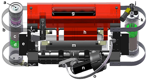
Figure 1The principal components of the next-generation C-OPS backplane with C-PrOPS (roll is the long axis and pitch is the short axis into or out of the page), as follows: (a) irradiance cosine collector; (b) radiometer bumper; (c) array of 19 microradiometers; (d) aggregator and support electronics; (e) rotating V-block for pitch adjustment; (f) two-point harness attachment; (g) hydrobaric buoyancy chamber, which accommodates up to 3 compressible bladders; (h) slotted flotation and (i) bronze weights for buoyancy and roll adjustment; (j) water temperature probe and (k) pressure transducer port on the radiance end cap; (l) conductivity sensor; (m) electronics module; (n) digital thruster (one of two, on each side); and (o) thruster guard. The aggregator and support electronics control the 19 microradiometers as a single device. The side bumpers and thruster guards protect the radiometers and digital thrusters from unanticipated side impacts, respectively.
The two digital thrusters have the same cant angle with respect to the vertical, which directs the weak turbulence from the thrusters downward and below the irradiance instrument, thereby ensuring both light apertures are observing undisturbed water; the opposite occurs if thrust is reversed. To steer the backplane like a remotely operated vehicle, differential thrust is applied to the two thrusters (Hooker et al., 2018a) and allows for real-time positioning adjustments, which is a significant advantage in shallow waters, e.g., away from a shoreline or within a wetland.
Once the profiler reaches the desired position for obtaining a vertical profile of measurements, or cast, it is kept in position by maintaining weak forward thrust. While at the surface, the pressure transducer measures atmospheric pressure right before a profile commences, which allows a pressure tare for every cast and improves the accuracy of depth measurements (Hooker, 2014). The pressure transducers used herein have a depth resolution, in terms of precision, of 0.03–0.08 mm in all water masses. When thrust is removed, the thruster-induced bias in the roll axis relaxes (the pitch angle is negligible, because prior thrust aligns the backplane with almost no pitch angle), and the profiler descends with stable tilts (Hooker et al., 2018a). Unlike rocket-shaped profilers (Hooker et al., 2001), the profiler has no significant righting moment and the planar orientation of the radiometers is maintained from the start of data acquisition, which significantly improves the VSR. In deep waters, the thrusters are used at the bottom of the cast to reduce the time between casts; in very shallow waters, the profiler was hauled closer to the surface before the thrusters were used to prevent resuspension of bottom material. All profiles were obtained in waters wherein the 10 % light level was above the bottom depth to ensure all data products were uncontaminated by bottom reflections.
Seven different instrument suites including a next-generation hybrid-spectral profiler with fixed wavelength and hyperspectral detector components plus a C-PrOPS (Hooker et al., 2018b) were used for this study. The fixed-wavelengths of the radiometers had similar configurations such that all measured the same nine spectral end-members from 320 to 412 and from 670 to 780 nm, plus six common wavelengths (Table 1). All optical instruments were calibrated at the same manufacturer facility with traceability to the National Institute of Standards and Technology (NIST) as described by Hooker et al. (2018b). NIST traceability is a requirement of the NASA Ocean Optics Protocols (hereafter, the protocols). The protocols set the standards for calibration and validation activities (Mueller and Austin, 1992), which were revised (Mueller and Austin, 1995) and updated over time (Mueller, 2000, 2002, 2003).
Table 1The nominal fixed wavelengths in nanometers, all with 10 nm bandwidths, for each optical profiling system as distinguished by serial number. The number of casts obtained is differentiated between backplanes without (C-OPS) and with (C-PrOPS) digital thrusters (note system 021 had both), wherein boldface numbers indicate the 15 wavelengths common to all profiling systems, e.g., 320 and 780 nm.
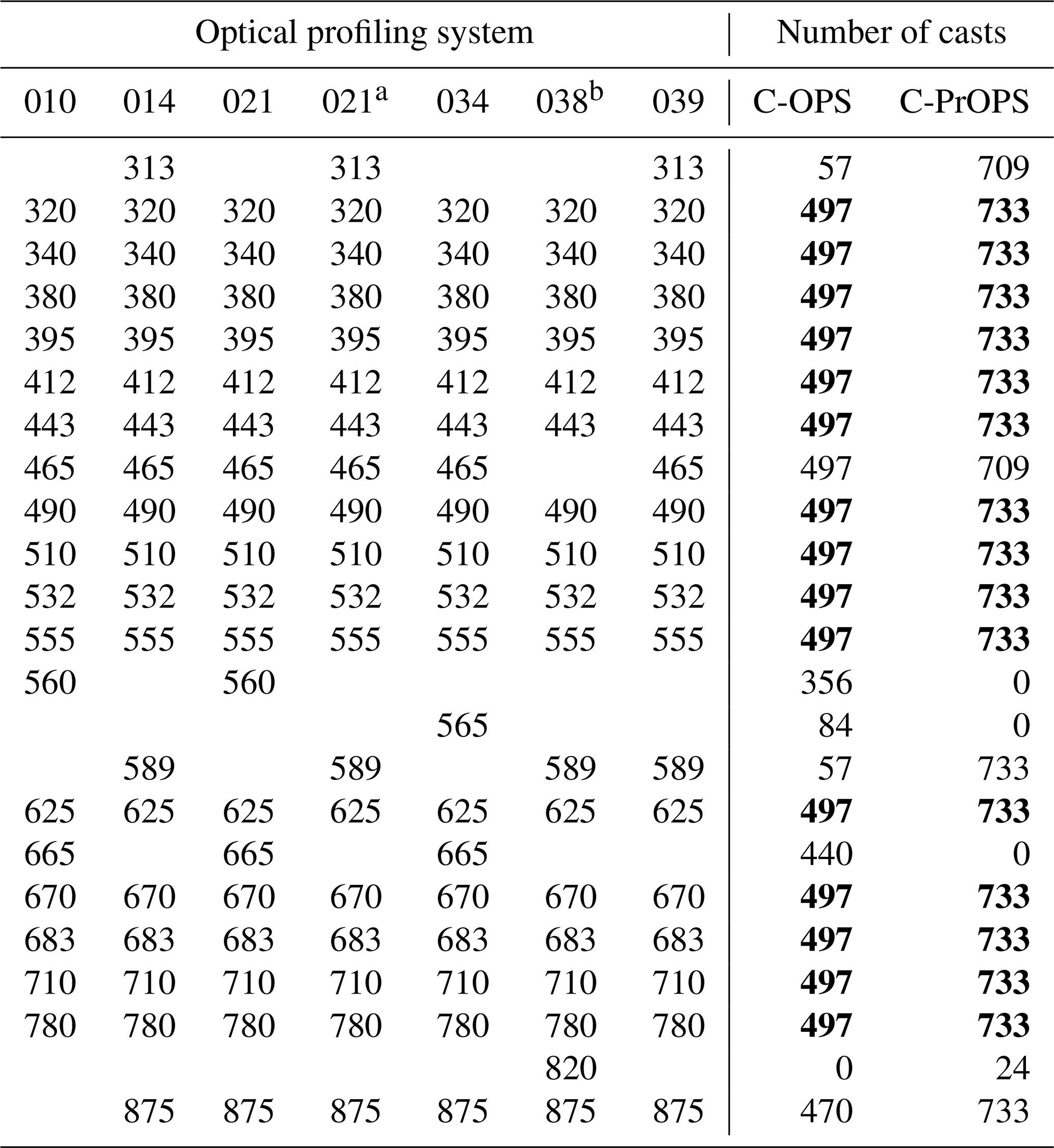
a Upgraded with C-PrOPS, a conductivity sensor, and new wavelengths. b Hybrid spectral and equipped with C-PrOPS.
A comparison of C-OPS acquisition with and without thrusters (Hooker et al., 2018a) verified the former improved efficiency in all waters by a factor of 2 or more, and either no or minor adjustments to the extrapolation interval used to derive data products for replicate casts were needed (thrusters minimize the negative influences of heterogeneity across all wavelengths). The improved efficiency yields a closer temporal matchup between the collection of optical profiles and the water sample. Approximately 98 % of water samples were obtained from the surface using a bucket. For some inland waters, the profiler was launched from a shoreline or dock, for example, when the boat ramp was out of service (due to drought, flooding, invasive species regulations, etc.). If a water sample could not be otherwise retrieved from the profiling location, the Compact-Profiler Underway Measurement Pumping System (C-PUMPS) was used (Hooker et al., 2018a). C-PUMPS provides a 20 mL s−1 flow rate from the profiler and fills a 1 L container in less than 1 min.
2.2 Field sampling
The Hooker et al. (2013) study area was the Beaufort Sea in proximity to the Mackenzie River outflow, the Gulf of Maine, and the vicinity, including major portions of its inland watershed plus minor watershed drainage from smaller rivers and a saltwater marsh. A validation data set from observations made in US coastal waters within the southern Mid-Atlantic Bight was also used. Neither of the two data sets included typical lacustrine water masses. The new sampling area for the study herein included the western US (i.e., California, Oregon, Washington, Nevada, Utah, and Idaho), Hawaii, Puerto Rico, Japan, the western North Pacific Ocean (e.g., the Kuroshio and Oyashio currents), the central North Pacific Ocean, the Bering Sea, the Chukchi Sea, and the Beaufort Sea (Fig. 2). The last is the only region that slightly overlaps the Hooker et al. (2013) study. The new data set includes sampling in a wide diversity of inland rivers, lakes, and reservoirs, including hypersaline and alkaline lakes.
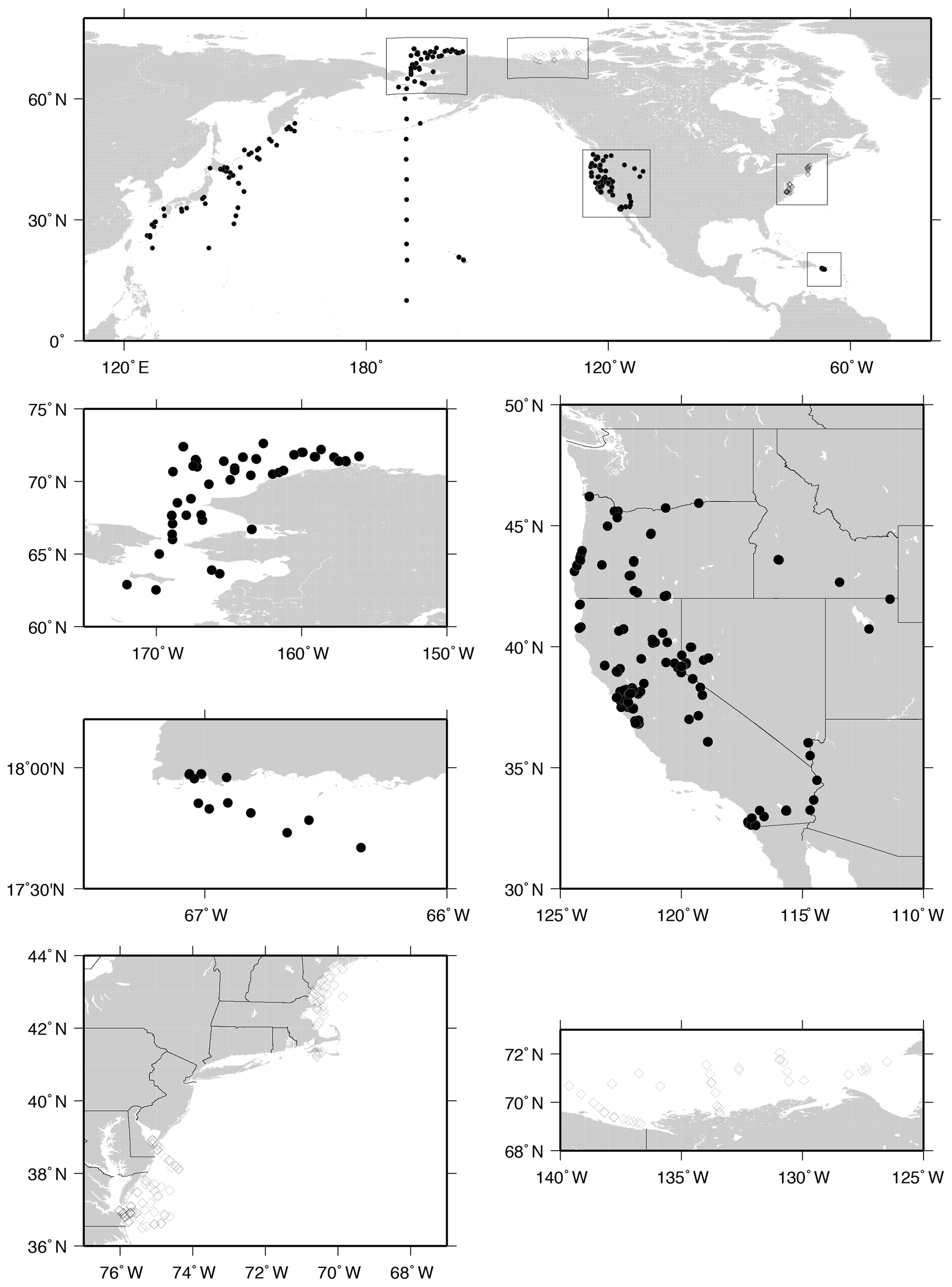
Figure 2The geographical distribution of the original Canadian Arctic and US east coast data (open diamonds) used in Hooker et al. (2013) versus the new data used herein (solid circles).
The new field data are divided into the aforementioned three primary categories according to whether or not the sampling station was in the open ocean, coastal zone, or inland waters. The open ocean is defined as offshore waters with a water depth exceeding 200 m. The coastal zone includes nearshore bathymetry of 200 m or less, wherein the adjacent saline waters and shoreland strongly influence each other, and includes islands, bays, deltas, transitional and intertidal areas, salt marshes, wetlands, beaches, etc. Inland waters are all other water bodies landward of the coastal low-water line, which are predominantly – but not exclusively – fresh lacustrine and riverine ecosystems.
Twenty-five campaigns spanning from 29 April 2013 to 25 January 2017 were conducted with 318 stations occupied and 1230 vertical profiles obtained, which were executed as a minimum of three sequential casts at each station. A majority of the optical data (733 casts) were obtained with C-PrOPS (Table 1) in all three primary categories, whereas optical sampling without thrusters (497 casts) was almost exclusively in the open ocean and coastal bays with minimal heterogeneity and deep mixed layers. Duplicate, and sometimes triplicate, water samples were collected at each C-PrOPS station. For open-ocean campaigns in the Pacific Ocean and Arctic, which included some coastal waters, a single seawater sample was usually collected. A selected volume of each water sample was filtered through a 0.22 µm filter under a gentle vacuum and collected in appropriate (e.g., pre-combusted) clean glass vials or bottles. Typically, CDOM absorption was measured within a few hours after sampling. In some cases when this was not possible, samples were stored at −20 ∘C or less until subsequent laboratory analysis at a shore facility (Sect. 2.4). While Fellman et al. (2008) reported that freezing changed the chemical composition of DOC for freshwater (stream) samples, Hancke et al. (2014) found no such effect for Arctic marine samples, nor was any systematic bias observed between the subset of frozen samples compared to the full suite of samples used for this analysis.
The surface water sample was obtained as quickly as possible after three optical casts were performed. In some cases when the heterogeneity or turbulence of the water mass was considered to be excessive, an additional three optical casts were executed immediately after the water sample was collected. The determination of excessive conditions was based on the stability achieved in optical variables (e.g., the average vertical tilt in the upper 2 m of the water column, changes in the 10 % light level depth) during data acquisition for the first three casts.
2.3 Optical data processing
All optical data products discussed herein, e.g., Kd(λ), were estimated in a near-surface interval of the water column with homogeneous properties as confirmed with physical data and analysis of the linearity of extrapolations provided by the processing scheme. The processor used here is based on a well-established methodology (Smith and Baker, 1984) that Hooker et al. (2001) showed is capable of agreement at the 1 % level within an international round-robin, when the processing options are as similar as possible and both data acquisition and processing strictly adhere to the protocols. Summary details of the data acquisition and processing capabilities are provided in Antoine et al. (2013), Hooker (2014), and Hooker et al. (2018a, b, c), so only brief overviews are presented herein.
In-water radiometric parameters in physical units are normalized with respect to separate, but simultaneous, measurements, with t expressing time dependence. After solar normalization and ±5∘ tilt filtering, a near-surface homogeneous portion of Ed(z,λ) centered at depth z0 and extending from and is established separately for the blue–green and red wavelengths; the UV and near-infrared (NIR) wavelengths are included in the blue–green and red intervals, respectively. Both intervals begin at the same shallowest depth, but the blue–green interval is allowed to extend deeper if the extrapolation linearity, as determined statistically, is thereby improved (this only occurs in oligotrophic, optically simple waters with deep mixed layers). The negative value of the regression slope yields Kd(λ), which is used to extrapolate the fitted Ed profile to null depth ().
A principal benefit of profile data with a high VSR is that the aliasing caused by wave-focusing effects (Zaneveld et al., 2001) can be significantly reduced during data processing. The separately obtained above- and in-water Ed values at and , respectively, can be compared using
where the constant 0.97 represents the applicable air–sea transmittance, Fresnel reflectances, and the irradiance reflectance (Morel et al., 2007). The distribution of light measurements at depth z influenced by wave-focusing effects does not follow a Gaussian distribution, especially during clear-sky conditions, wherein the amplitude of the brightened signals exceeds the companion darkened signals. Consequently, arithmetic averaging is not appropriate and linear fitting of Ed in a near-surface layer is poorly constrained, especially if the number of samples is small.
The appropriateness of the Ed extrapolation interval, initially established by z1 and z2, is evaluated by determining if Eq. (1) is satisfied to within the 2.3 %–2.7 % uncertainty (k=2 coverage factor) of the optical calibrations (Hooker et al., 2018b); if not, z1 and z2 are redetermined – while keeping the selected depths within the shallowest homogeneous layer possible – until the disagreement is minimized (usually to within 5 % to include some inevitable variance from natural processes to the calibration uncertainty). In this procedure, selection of the near-surface extrapolation interval uses a boundary condition or constraint (Antoine et al., 2013), wherein the central tendency of the distribution of data within the extrapolation interval, which are typically subjected to wave-focusing effects, satisfies Eq. (1).
The linear decay of all light parameters in the selected near-surface layer is then evaluated, and if linearity is acceptable, the entire process is repeated on a cast-by-cast basis. Subsurface quantities at null depth are obtained from the slope and intercept given by the least-squares linear regression versus z within the extrapolation interval specified by z1 and z2. A secondary benefit of profile data with a high VSR is that the extrapolation interval can have a restricted vertical extent, but still have sufficient data to satisfy Eq. (1) and produce data products at all wavelengths. This is an important advantage in optically complex water masses, which are frequently turbid and shallow.
2.4 Water sample processing
For the Pacific Ocean samples and approximately half of the Arctic samples, the absorption spectrum of CDOM was determined using a spectrophotometer (Shimadzu UV-1800) according to Yamashita et al. (2013). Briefly, after the water sample was thawed and reached room temperature, the spectral absorbance was measured from 200 to 800 nm at 0.5 nm intervals with a 10 cm quartz-windowed cell. Absorbance spectra of a blank (Milli-Q water) and samples were obtained against air, and a blank spectrum was subtracted from each sample spectrum. The blank-corrected absorbance spectrum was baseline-corrected by subtracting average values ranging from 590 to 600 nm (Yamashita and Tanoue, 2009) and then converted to the absorption coefficient (Green and Blough, 1994). A single absorbance analysis was generally carried out for the open-ocean samples, with an average accuracy from replicates of 2.5 %.
For the other Arctic samples, CDOM absorption coefficients were determined using an UltraPath liquid waveguide (Matsuoka et al., 2012, 2017). Briefly, CDOM absorbance for a filtrate (less than 0.2 µm) was measured relative to a reference water within a few hours after sampling. The reference water was prepared in advance using pre-combusted pure salt (450 ∘C for 4 h) with Milli-Q water to adjust salinity within ±2 between a sample and a reference to correct for the refractive index effect. A 2 m optical path was used for all waters except some coastal sites wherein a 0.1 m path was used (Matsuoka et al., 2012, 2014). After baseline correction, absorbance was converted into absorption coefficients by including the optical path length. The detection limit was within 0.001 m−1 (Matsuoka et al., 2017).
For the western US coastal and inland waters, water samples were passed through a 0.2 µm syringe filter (Whatman GD/X), and absorbance of CDOM was measured on either a Cary Varian 50 spectrophotometer using a 10 cm quartz cell or an UltraPath liquid waveguide spectrometer with a 2 m path length. The syringe filter was rinsed with sample prior to collection, with the sample stored in an amber, acid-washed, and combusted (450 ∘C for 4 h) glass vial with Teflon septa and kept in the dark at 4 ∘C until analysis. Absorption spectra of the filtered samples were measured using ultrapure water from a Millipore Milli-Q A10 pure water system with UV to reduce total organic carbon to less than 10 ppb. The absorption coefficient (calculated as absorbance divided by path length, multiplied by 2.303 to convert to natural log units) at 440 nm representing CDOM abundance was estimated using the single exponential model (SEM) for absorption from 300 to 700 nm as described by Twardowski et al. (2004). The three different methods used in this study for determining CDOM absorption do not influence the results (see a sensitivity analysis in Sect. 4). For all the CDOM data – regardless of the collection and processing method – the spectral slope for the wavelength range 350–500 nm was calculated by fitting a nonlinear least-squares model to aCDOM(λ).
2.5 Data subcategories
Algorithm validation requires an assessment prior to data collection whether or not the sampling violates the assumptions made to create the algorithm. For this study, water masses wherein the evolution of aCDOM(440) or Kd(λ) was considered conservative, i.e., within the likely range in the gradient of such properties because no stressors to challenge that perspective were evident, are considered validation quality with primary categories of open ocean, coastal zone, or inland waters. Those water masses thought to contradict the algorithmic approach, because one or more stressors challenging the conservative evolution perspective were evident prior to sampling, were subcategorized to exclusively assess algorithm performance as more complex water masses are included in validation, as follows.
-
Waters closer to an ice field contain meltwater properties, which freshen the neighboring water body and can result in additional particles or compounds not usually found in the parent water mass.
-
Waters farther from an ice field, but within proximity, contain lesser amounts of meltwater properties.
-
Resuspension occurs naturally when a sufficient flow (e.g., an ebb or flood tide) or turbulent wave field (e.g., created by sufficiently strong winds) interacts with shallow bottom sediment to create concentrations of constituents that would otherwise not be present; it occurs unnaturally when a boat propeller (or other mechanical device) churns up shallow bottom sediment (e.g., in a harbor, marina, or navigation channel).
-
A refilled lake experiences a rapid inflow of alluvium (e.g., gravel, sand, silt, and clay) from riverbeds and eroding banks, plus floating and partially submerged debris, which can also resuspend bottom sediment. If the refilled lake is a controlled reservoir and exceeds the normally maintained fill level, new lake bottom is added, which can be a source for additional, perhaps atypical, water constituents in terms of type or concentration.
-
A drought-stricken lake has a longer residence time (the amount of time for the time-elapsed outflow to equal the lake volume) than normal, because once the water level remains below the overflow elevation, evaporation and ground seepage are the primary outflows. Increased residence time can concentrate constituents, plus dried and exposed bottom material can be resuspended into the shrinking lake volume due to wind or rain.
-
A harbor (or marina) is a docking facility, usually in shallow water, for vessels of varying sizes. Such facilities can be a source of pollutants and bottom resuspension and typically include structures (breakwaters, jetties, piers, etc.) for shelter from severe weather, which can alter residence times by restricting water exchange.
-
A harmful algal bloom (HAB) is a toxic or noxious algae in a concentration producing a deleterious effect on humans or the environment. HABs are usually influenced by chemical, physical, and biological factors.
-
A wetland (plus marsh or mangrove) filters dissolved and suspended water constituents (e.g., from tidal cycles, weather events) through settling and plant consumption but might not completely remove them.
-
A polluted water mass is contaminated from an anthropogenic source that alters the natural water properties.
-
An alkaline (or soda) lake has limited biodiversity due to an elevated pH of 9–12 with high carbonate and complex salt concentrations affecting the solubility and toxicity of chemicals and heavy metals (Grant, 2006).
-
A hypersaline lake contains high concentrations of sodium chloride (or other salts) surpassing seawater, which limits biodiversity to organisms tolerating high saline levels (e.g., Mono Lake had a salinity of about 50).
-
A river mouth is where significant amounts of alluvium are deposited into a larger water body (e.g., a delta).
-
An atypical bloom is a generic case of high biomass based on local reports evaluated with respect to typical temporal and spatial conditions, which may involve weather effects (e.g., wind) concentrating algae advectively.
-
An invasive species is an introduced plant, fungus, or animal that is not native to a water body and is anticipated to alter the heretofore established properties and perhaps with a significantly negative outcome (e.g., damage to the environment, economy, or health of organisms, including humans).
-
A parent water mass modifier is a localized alteration of water properties, e.g., a creek inflow into a lake, and demonstrates the sensitivity of the methods used herein to distinguish small changes.
The above 15 subcategories plus the original validation quality category results in 16 categorizations, and as the former more complex waters are incrementally added to the latter, quantitative cause-and-effect validation scenarios are created (Sect. 4). If a sample was applicable to more than one subcategory, e.g., a wetland can experience resuspension from tidal currents, a dominant subcategory was selected based on observations prior to sampling. Categorization ambiguities are not worrisome, because complex water masses are a small fraction of global ecosystems.
The proximity to ice (farther and closer) subcategories is based on the relative position of safely operating a small vessel in and around an ice field. Sampling was usually as close to the ice as possible and then as far from the ice within line of sight of the larger ship the small boat was launched from. In comparison, categorizing a refilled lake is a straightforward comparison of the water level datum available from local authorities with respect to the outflow elevation and historical norms. All refilled lakes were at 100 % capacity or more; for example, Washoe Lake was overfilled.
The categorization of bottom resuspension is primarily based on visual evidence, wherein resuspended particles are visible and produce a significant change in water color (e.g., Akkeshi Bay after the passage of typhoon Vongfong). Although a subset of sampling obtained in harbors could be classified as resuspension stations, a harbor (or marina) is identified based on local identification of such facilities. Similarly, wetlands (plus marshes and mangroves) are identified based on navigation charts, maps, and local descriptions. Hypersaline (endorheic) lakes are similarly categorized by state and local authorities (e.g., Mono Lake, Great Salt Lake, and Salton Sea), as are alkaline lakes (e.g., Mono Lake, with dual classification, plus Borax Lake and Soda Lake).
Categorizing drought-stricken lakes relies on local authorities reporting lake elevations and inflow water volumes with respect to historical norms. Examples from 2015 are as follows: (a) Shasta Lake water storage was 56 % below normal, (b) Lake Almanor was 118.5 ft (36.1 m) below normal elevation, (c) the Truckee River flow into Pyramid Lake (Nevada) was near historical lows and was dry for 3 d prior to sampling, and (d) Eagle Lake had a water level of 5091.5 ft (1551.9 m), which was within 0.5 ft (0.2 m) of the lowest level recorded in 1935.
The categorization of a river mouth is a combination of the geographical location (e.g., the Columbia River) and evidence of the presence of the water mass the river flows into (e.g., salt water intrusion from the nearshore bay). The inflow of smaller rivers, streams, and creeks into a larger water body (e.g., Ward Creek flowing into Lake Tahoe) is not classified as river mouths, but rather as parent water mass modification from a creek inflow. The creek designation is to ensure the understanding that the inflow volume is small, but the expectation is changes in water properties are nonetheless discernible because of the enhanced sensitivity (e.g., VSR) of the methods used.
The categorization of a water mass subjected to pollution, an atypical bloom, HAB, or an invasive species relied principally on eutrophic chlorophyll concentrations plus historical reporting or on-site local representatives. The latter are frequently present at boat ramps to oversee measures to mitigate health concerns or prevent the spread of invasive species, which is presently a significant and escalating problem throughout the western US.
2.6 NOMAD archive
The NASA bio-Optical Marine Algorithm Dataset (NOMAD) v2.a (Werdell and Bailey, 2005) is a small, quality-controlled subset of a larger data repository established early in the Sea-viewing Wide Field-of-view Sensor (SeaWiFS) satellite mission (Hooker and Esaias, 1993) called the SeaWiFS Bio-Optical Archive and Storage System (SeaBASS) and is described by Hooker et al. (1994). The NOMAD database does not include applicable aCDOM(440) measurements with contemporaneous UV and NIR spectral end-members as used in this study. Consequently, the Hooker et al. (2013) algorithmic approach, which is based on UV and NIR end-members, cannot be evaluated.
The NOMAD database, however, does include Kd(λ) with legacy visible (VIS) wavelengths plus a matching dissolved (gelbstoff) spectral absorption coefficient at 443 nm, ag(443), which is functionally equivalent to aCDOM(443) following Röttgers and Doerffer (2007). The consequences of the 3 nm shift in ag(443) with respect to aCDOM(440) are considered negligible for a generalized inquiry involving legacy optical data, because the fixed wavelengths involved have 10 nm bandwidths and there are multiple sources of uncertainties in the derived data products of equal or greater importance (Hooker et al., 2013), e.g., pressure tares, aperture offsets, dark currents, wave focusing.
2.7 Alternative classification scheme
The subcategory scheme (Sect. 2.5) included factual knowledge combined with careful inspection regarding one or more significant constituents or stressors influencing water mass complexity. Previous studies applied fuzzy c-means (FCM) classification to ocean color algorithm development (Moore et al., 2001) or uncertainty estimation (Moore et al., 2015), thereby demonstrating the usefulness of the FCM over a crisp or hard (e.g., k-means) classification. Application of the FCM classification is to log-transformed Kd(λ) data based on the Calinski and Harabasz (1974) index (Matsuoka et al., 2013). All of the reported FCM classes are based on the water masses sampled herein, except the first class includes the influence of the Kd values of pure seawater, denoted Kw (Morel and Maritorena, 2001).
All data not categorized as one of the 15 subcategories prior to data collection (Sect. 2.5) are retained in the open ocean, coastal zone, and inland water primary categories to yield the following number of validation quality observations, respectively: 190, 223, and 196. This new filtered data set of 609 observations is reasonably balanced, because each primary category contains approximately 200 observations. These data are used to initially evaluate the global applicability of the original Hooker et al. (2013) aCDOM(440) algorithm. The comparison of the new validation quality data (i.e., data not part of the 15 subcategories) with respect to the original algorithm is presented in Fig. 3. The enhanced global sampling of the new data set with respect to Hooker et al. (2013) yields the following distinctions: (a) the addition of lacustrine water bodies (including Lake Shikotsu in Hokkaido, Japan), which almost span the entire 3 decades of dynamic range (e.g., Crater Lake to Pinto Lake), and (b) the expansion of the dynamic range to include clearer and more turbid water masses, which also means deeper and shallower waters.

Figure 3The new validation quality data from the primary open ocean, coastal zone, and inland water (blue, green, and red circles, respectively) categories, which are used to evaluate the original Hooker et al. (2013) algorithm (gray circles). The location names of a subset of observations are explicitly identified as a function of the approximately 3 decades of dynamic range in both axes. A ±7.5 % dispersion is approximately represented by the larger algorithm symbol size; i.e., from one edge of a gray circle to the opposite edge represents a total of approximately 15.0 % dispersion. The headwaters of the San Francisco Bay Redwood Creek (RWC) channel, which is surrounded by wetlands, is the most turbulent coastal water mass and has the highest aCDOM(440) value.
Given the diversity of sampling in this study, it is unlikely that the more than 3 decades in aCDOM(440) data (Fig. 3) might nonetheless exhibit similar chemical composition; i.e., the quantity of CDOM varies but the type remains constant. To reject the latter, the Fig. 3 CDOM spectral slope, S, values were compared to a global compilation of marine CDOM estimates from over 500 oceanographic campaigns (Aurin et al., 2018). The new study reported a comparable spectral range (350–600 nm) and a median S of 0.0167 nm−1 with a range of 0.0090–0.0208 nm−1. In comparison, Fig. 3 data have a similar median of 0.0175 nm−1 and a slightly larger range of 0.0095–0.0410 nm−1. In addition, Grunert et al. (2018) compiled similar statistics by marine province, with a comparable result in spectral range (350–550 nm) and an approximate range in S of 0.01–0.05 nm−1. Consequently, the range of S presented in this study is comparable to similar recent global analyses spanning the majority of marine waters.
The new validation quality data significantly adhere to the original algorithm, as evidenced by how the red, green, and blue circles in Fig. 3 are well contained within the approximately ±15 % gray boundaries that denote the dispersion in the original algorithm. The category that spans the largest percentage of the dynamic range for both axes is the inland water data, although the coastal zone is somewhat similar because of the clear Hawaiian coastal waters that were sampled. The open-ocean category has the smallest dynamic range, but this does not diminish the importance of this category because it represents the greatest surface area and volume of water on the planet.
The new data values, Vn, are compared to the corresponding algorithm value, with the latter being the reference values, Vr, in the comparison calculation. The relative percent difference (RPD) between the new data and the algorithm is computed as RPD and is expressed as a percent. The average RPD for all the new data is 0.02 %; i.e., the new data show a negligible bias with respect to the original algorithm. The absolute percent difference (APD), which provides an estimate of the dispersion of differences between the new data and the algorithm, is the absolute value of the RPD. The average APD value for all the new data is 3.9 %; i.e., the new validation quality data are usually to within 5 % of the original algorithm (as visually confirmed by Fig. 3).
3.1 Drought-stricken, alkaline, hypersaline, and refilled lakes
The new lacustrine data are presented in Fig. 4. Data from the hypersaline and alkaline (endorheic) lakes do not conform with the algorithm. Drought-stricken lakes exhibit a wider range of departure, with the most significant occurring for the most depleted water bodies, e.g., Lake Almanor and Shasta Lake. Endorheic drought-stricken lakes, e.g., Eagle Lake and Pyramid Lake, are the most extreme. Refilled lakes also do not conform with the algorithm, and refilled drought-stricken lakes exhibit an increase in CDOM and turbidity, e.g., Shasta Lake and Pyramid Lake.
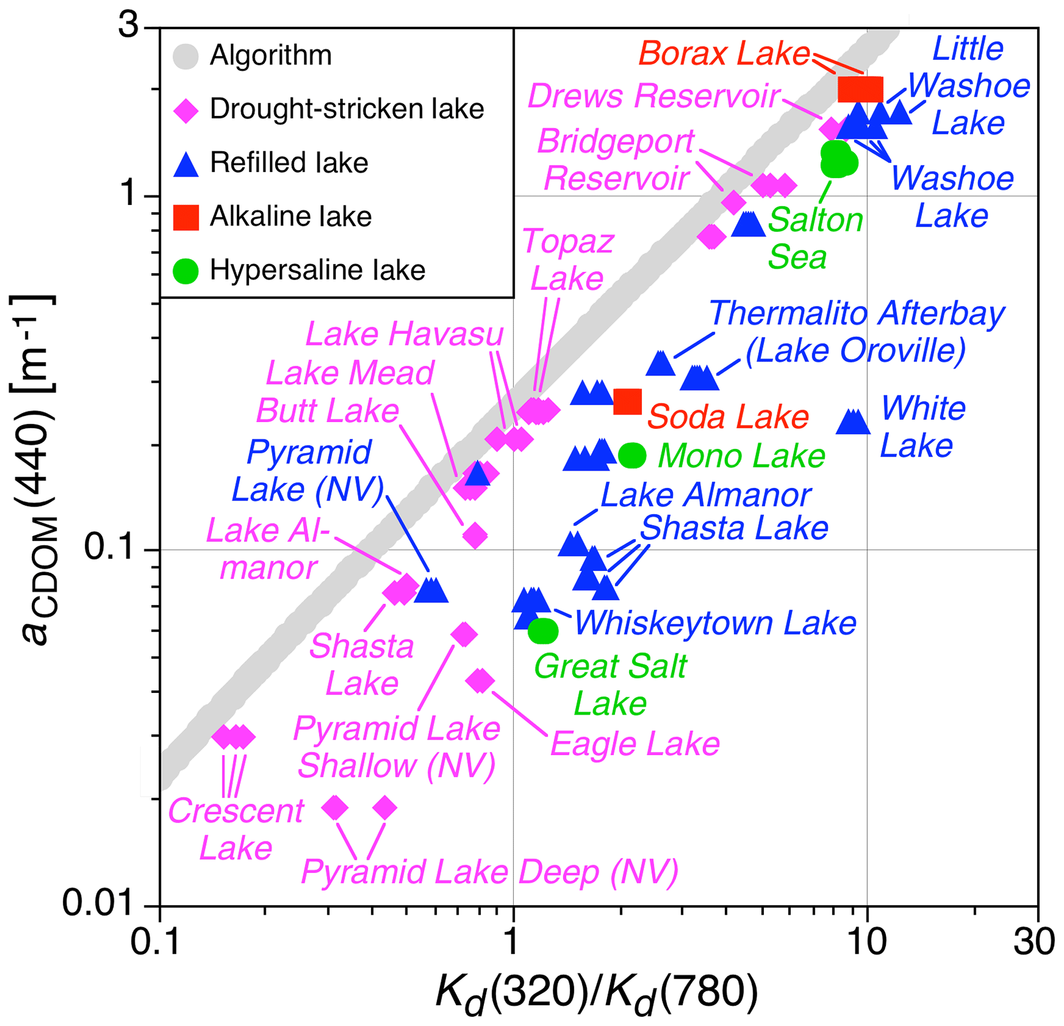
Figure 4The new data from lacustrine water bodies that were drought-stricken (magenta diamonds), refilled after drought (blue triangles), alkaline (red squares), or hypersaline (green circles) in relation to the original algorithm (gray circles). Each data point represents a single water sample with multiple optical casts for each, which results in a series of results (typically three to six) along the x axis.
The refilled lakes in Fig. 4 are frequently more different with respect to the algorithm than hypersaline or alkaline lakes, especially in terms of turbidity as determined by the Kd ratio. This is because some of the refilled lakes are overfilled, wherein the shore of the lake extends beyond the normal acreage of the lake (e.g., Washoe Lake and Little Washoe Lake). In overfilled lakes, land that is not normally flooded is added as new lake bottom, and the new acreage is a source of atypical constituents, in either composition or concentration (e.g., atypical constituents from land-use activities can be added when a lake overfills, because these activities are not possible in the water mass). The refilling of a normally dry endorheic basin, e.g., White Lake, wherein the flood waters and the reclaimed lake bottom provide the maximum areal and volumetric source of dissolved and suspended constituents, results in some of the most extreme results, in terms of both turbidity and the algorithm.
The discharge from overfilled reservoirs also has significant deviations with respect to the algorithm. Thermalito Afterbay receives the discharge from Lake Oroville and was sampled after the overfilling of the parent water mass during the drought-breaking California 2016–2017 winter. Data were obtained in two locations, with higher CDOM data obtained in a shallow marsh. The ability to distinguish small localized differences establishes the sensitivity of the methods used herein. For example, the three refilled Shasta Lake samplings in Fig. 4 were conducted in different locations subjected to the inflow of a creek, as well as a large floating and partially submerged debris field.
3.2 River mouth, resuspension, and ice edge proximity
The inflow of dissolved and suspended constituents to a parent water mass is explored further by considering a variety of sources that can add to water mass complexity. The new data are shown in Fig. 5 and were obtained in river mouths, water bodies with known suspension or visible resuspension, plus samples obtained closest to or farthest from the ice edge within an oceanic ice field. Water bodies with known suspension or visible resuspension are primarily from tidal and riverine flows, which are shown in Fig. 5 as triangles. Almost all of the resuspension data were obtained at peak tidal flow to ensure safe navigation in the necessarily shallow waters. The Akkeshi Bay data were obtained the day after the passage of typhoon Vongfong, wherein the shallow bay waters were a distinctly different color than normal. The Sacramento River data were obtained after heavy rains, wherein the boat ramp to be used was closed due to flood waters. The difference between the flooded Sacramento River with respect to the inland riverine data in Fig. 3 not in flood conditions (i.e., as conservative water masses) shows the classification of the Sacramento River is appropriate and the subjective classification approach has merit.
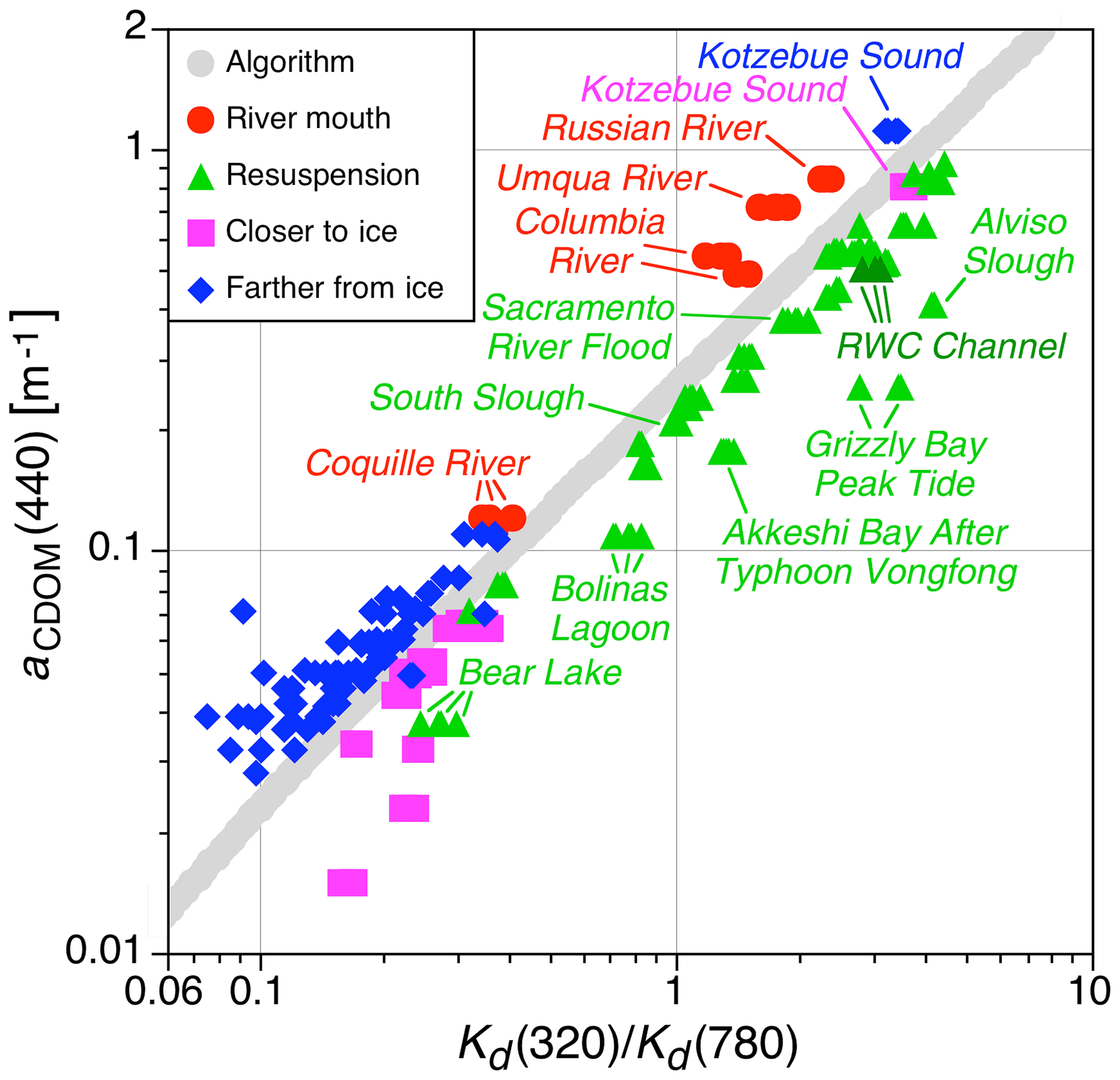
Figure 5The new data obtained in river mouths (red circles), water bodies with known suspension or visible resuspension (green triangles), plus samples obtained closer to (magenta squares) or farther from (blue diamonds) the ice edge within an ice field. The San Francisco RWC channel headland waters are depicted in Fig. 3 as are the Columbia and Umpqua river data that are upstream of the river mouth.
The resuspension data in Fig. 5 also include Bear Lake (which straddles the Utah–Idaho border) plus the effects of a large ship docking in the shallow RWC channel with the aid of a tugboat. The latter involved the churning up of bottom material that significantly changed the color of the water. The resuspension sampling occurred shortly after the ship was docked. The Bear Lake scattering anomaly is created primarily through groundwater seepage, which is rich in calcium carbonate particles (Davis and Milligan, 2011). The groundwater is nutrient poor and the small amount of riverine input to the lake is through a swamp and wetlands, wherein plants consume the nutrients and sediments settle out. Consequently, the Bear Lake data represent a significant clear-water scattering anomaly.
The other clear-water data in Fig. 5 were obtained principally in proximity to Arctic oceanic ice fields and are distinguished as being closer to, or farther from, the ice. These data are displaced above or below the algorithm, even in the turbid waters of Kotzebue Sound. The majority of these data were obtained using a small boat launched from a larger ice breaker, so the data obtained closer to the ice are as safely close to the ice as possible while being beyond the shading of the water mass by the ice field. The classification of closer to and farther from is qualitative, and in complicated ice fields misclassification is possible. The Fig. 5 data show only two farther from points that are likely not classified correctly, and this category is the most vulnerable to a qualitative error.
In regards to the resuspension data, which all cluster below the algorithm in Fig. 5, river mouth data are the opposite – the data cluster above, but the number of such observations is much smaller. The reduced number is due to the difficulty of operating a small boat on a trailer in a shallow river and then safely navigating the vessel out into the river mouth through a frequently narrow channel, wherein the higher sea state of the coastal ocean can be significantly amplified, and boat traffic can make station work hazardous. Within the plume of a river mouth, two usually rather different water masses meet and mix over short timescales. Under those conditions, short-term deviations, with respect to the algorithm, can emerge, as shown in the Fig. 5 data.
3.3 Atypical blooms, invasive species, and harbors
The presence of an atypical bloom, particularly a HAB, is anticipated to create additional optical complexity, because one or more significant stressors are frequently involved, e.g., an overabundance of nutrients, which can be anthropogenic in origin (Heisler et al., 2008). In a generic context, an atypical bloom includes the concentration of biomass to artificial levels (Kudela et al., 2015), perhaps due to local weather, (e.g., advective processes from winds and waves). Invasive species and harbors are also expected to increase optical complexity.
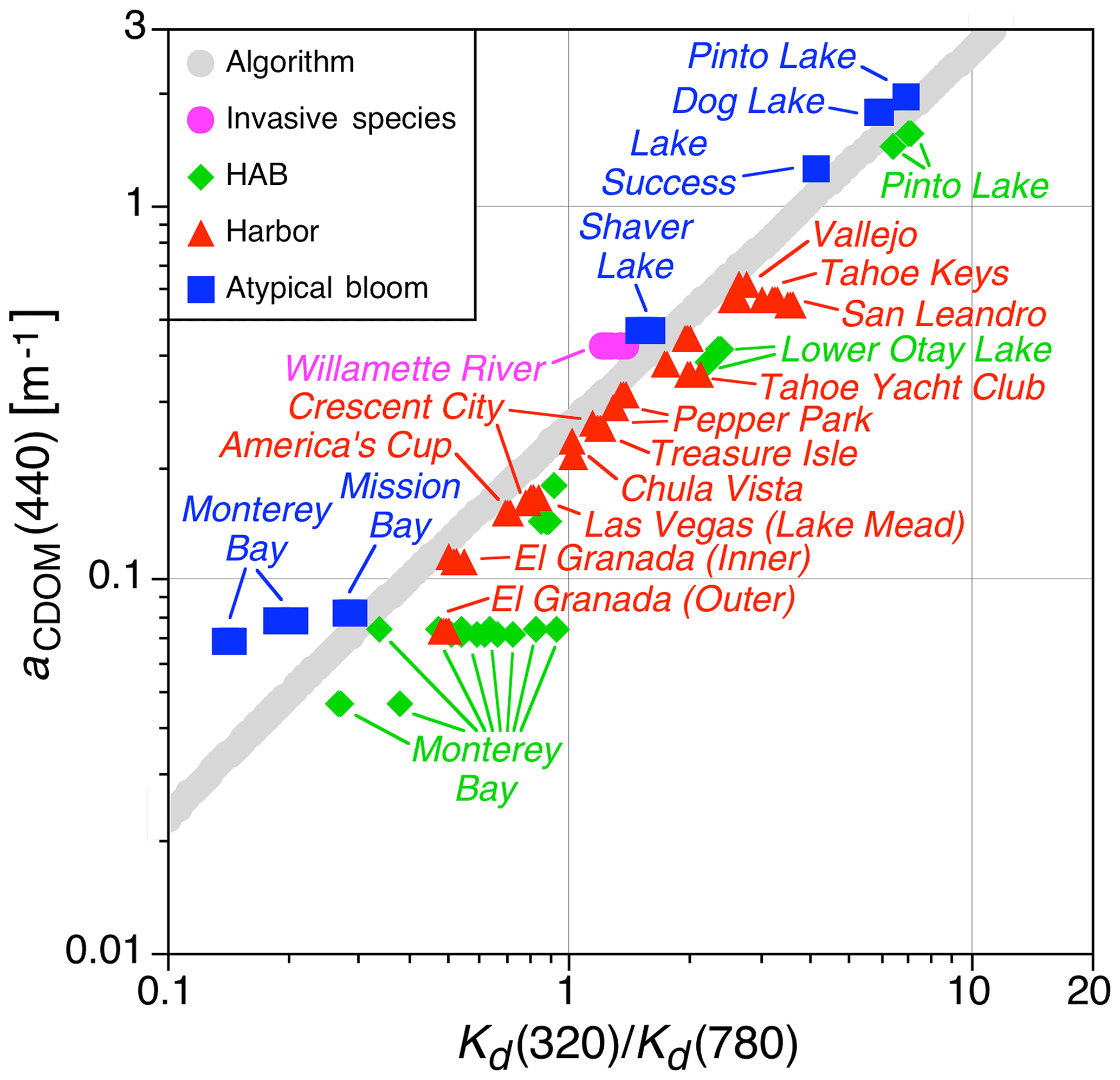
Figure 6The new data obtained in a harbor (or marina), plus water bodies experiencing an invasive species, HAB, or atypical bloom.
The new data obtained in harbors and water bodies experiencing an invasive species, or atypical bloom, including a HAB, are shown in Fig. 6. Some of these data could have had two classifications. For example, the Tahoe Keys and Tahoe Yacht Club were both infested with an invasive aquatic plant. Limited presence in one and mechanical removal in the other implied a harbor subcategory was appropriate. The Willamette River data were from an invasive aquatic species area (Bierly et al., 2015), and the algorithmic relationship is opposite that of the Lake Tahoe harbors. The latter suggests the Lake Tahoe harbor classifications, which cluster with the other harbors, are likely appropriate.
Almost all harbors exhibit elevated aCDOM(440) values with respect to the adjacent parent water mass, e.g., Chula Vista, Treasure Isle, San Leandro, and America's Cup. The relationship of harbors with respect to the algorithm has few extreme values, which is expected because harbors exchange water with the parent water mass. San Leandro and El Granada have the largest expression, but San Leandro is in a heavily urbanized area immediately south of Oakland International Airport in the San Francisco Bay area, so significant anthropogenic sources are anticipated.
Like some coastal harbors, El Granada vessels are moored in an inner shallow harbor protected by an outer deeper area, with both perimeter breakwaters and narrow channels. The two harbor areas cannot exchange water completely (i.e., a portion of the water volume is trapped during each tidal cycle) and are more turbid than the parent water mass, Half Moon Bay. The inner harbor is a likely and persistent anthropogenic source with a longer residence time, so it is anticipated to have an aCDOM(440) value exceeding the neighboring bay. The increased residence time and reduced exchange rates through the narrow channels are a possible mechanism to increase aCDOM(440). Other harbors wherein a protected moorage has elevated aCDOM(440) include Las Vegas (Lake Mead) and Crescent City.
The HAB data in Fig. 6 were frequently obtained opportunistically and, thus, were not necessarily from the peak of the phenomenon. Also, a bloom is heterogeneous and navigation within the bloom is mostly based on visual observations, so the relationship with respect to the algorithm is not always extreme. The Monterey Bay HAB data are the most extensive, because there was the opportunity for scheduling some of the data collection during a time period when a HAB was likely to occur. In all cases, a HAB observation has a larger Kd ratio than the algorithm predicts, and this is principally caused by an increase in the Kd(320) value, i.e., increased attenuation in the UV, which might indicate the presence of mycosporine-like amino acids (Jessup et al., 2009; Kwon et al., 2018).
An atypical bloom is primarily a combination of local reporting, and a heterogeneous eutrophic water mass, i.e., chlorophyll concentration exceeds 1 mg m−3, with some water bodies having concentrations greater than 10 mg m−3. Consequently, the lack of sophistication and specificity related to explaining this subcategory does not exclude a simpler explanation. For example, local wind conditions could elevate the values associated with a typical bloom into atypical concentrations. This phenomenon was observed in more than one lake, e.g., Pyramid Lake and Upper Klamath Lake. The majority of the atypical blooms are in rather close agreement with the algorithm.

Figure 7The new data obtained in a wetland or polluted water mass plus comparisons between a parent water mass and a creek inflow or another source of water properties.
3.4 Wetlands, pollution, and water mass modifiers
The new data obtained in wetlands or polluted waters are presented in Fig. 7. The former are almost all marsh grass except two, which are labeled according to their types. The two unlabeled types at the top of the plot are from Cutoff Slough in California and are marsh grass. All wetlands exhibit the same relationship; that is, they are all displaced above the algorithm, although four are in rather close agreement with the algorithm. The polluted water masses are associated with agricultural (Upper Klamath Lake and upper Elkhorn Slough) or mining (Clear Lake) runoff, with the latter being the most severe. For both Upper Klamath Lake and Clear Lake, blue–green algae were plainly visible with extreme maximum chlorophyll concentrations of 1.117 and 1.420 g m−3. The chlorophyll concentrations in upper Elkhorn Slough were less, but are still extreme with a maximum value exceeding 100 mg m−3.
Figure 7 also includes examples of a small inflow from a creek or another source modifying the neighboring parent water mass. These data provide a measure of the sensitivity of the data acquisition, processing, and analysis techniques used herein. Although other sensitivity examples are documented above, e.g., the distinction between sampling closer to, or farther from, the ice edge (Fig. 5), the Fig. 7 examples span diverse spatial scales, e.g., creek inflows, a fish kill in the Salton Sea, and a large floating and partially submerged debris field in Shasta Lake. In all cases, the anticipated algorithmic relationships appear different than the parent water mass. The water properties of the creek inflow are not known, because access to the source from a small boat was problematic.
The generalized properties of the inflowing creek waters, determined visually, are as follows: (a) the Lake Tahoe inflow was turbid, milky meltwater from snow and ice melting on shoreland; (b) the Shasta Lake inflow was from rocky, tree-covered terrain and was significantly clearer than the lake water (the water pooled into a small pond before flowing into the lake and was easily observed); (c) the Donner Lake inflow was from a rocky, tree-lined canyon; (d) the Mono Lake inflow was across a mostly barren, rock-strewn shore with loose soil and was notably brown compared to the green lake; and (e) the Pinto Lake inflow was from a densely vegetated buffer zone adjacent to farmland. The displacement of the modified waters with respect to the parent water mass is in keeping with these observations; i.e., the waters subjected to turbid or clear inflows had larger or smaller Kd(320)∕Kd(780) ratios.
3.5 Alternative spectral end-members
The end-member wavelengths used in alternative Kd(λ1)∕Kd(λ2) ratios, hereafter , follow the combinations first used by Hooker et al. (2013), i.e., the UV–NIR pair, as well as the VIS pair. Shortly after the start of this study, C-OPS system 021 was upgraded (Table 1), so the pair is also available and provides the widest spectral span (562 nm) between end-members. A plot of the end-member combinations is presented in Fig. 8, which also includes the linear fits and the root-mean-square error (RMSE) of the data with respect to the fits. The data in Fig. 8 are only those observations provided in Fig. 3; i.e., all 15 subcategories established in Sect. 2.5 (Figs. 4–7) are excluded. The consequences of using an increasing number of all the observations are presented in Sect. 4.
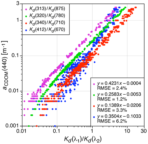
Figure 8Four end-member algorithms to derive aCDOM(440) from in-water optical observations with the accuracy of each (considering only a linear perspective) estimated using RMSE statistics.
The fits in Fig. 8 show the end-member pair with the best accuracy is , although the and fits are within the calibration uncertainty of the radiometers plus inevitable environmental variance, i.e., within 5 %. The slope of the fit is within 1.1 % of the original Hooker et al. (2013) algorithm (). As end-member wavelengths are brought spectrally closer together, the variance increases and reaches a maximum for the pair, which degrades accuracy (nonlinearity and RMSE generally increase with decreasing spectral separation of end-members). The RMSE is a little larger than for and a little less for . Fewer data creates gaps in the data distribution, which partially explains why these data do not yield the lowest RMSE.
The Fig. 8 data show the variance also increases after the transition from more turbid to clear waters, i.e., aCDOM(440)=0.02 m−1, and continues to increase with increasing water clarity. The larger variance as a function of water clarity is caused by the increasing importance of wave-focusing effects coupled with increasing NIR attenuation. Both problems are tractable for , but contribute to the difficulty of deriving data products and ultimately producing a stable . The increased and variances are not restricted to the problems described for . As end-members are brought spectrally closer together, the range of expression available to distinguish two similar but optically different water masses decreases. Consequently, choosing the extrapolation interval is more sensitive to small changes in the parameters that ultimately determine the fit for the extrapolation interval. For legacy end-members, clear waters have a lesser range of expression and turbid waters have the greatest, so this problem decreases as turbidity increases, which is seen in the and Fig. 8 data.
3.6 Legacy data archive
From the full set of 4459 NOMAD stations, 227 include end-members and ag(443) observations, hereafter aCDOM(440), but two are duplicates. Application of data to the corresponding algorithm in Fig. 8 results in 13 observations with negative (predicted) aCDOM(440) values, which are removed to leave 212 unique stations. This process demonstrates how end-member algorithms can be used to quality assure optical data in archives, although only a linear perspective is considered herein to maintain consistency with the algorithm. Of the 212 retained NOMAD stations, 189 are located within the Chesapeake Bay and its outflow into the southern Mid-Atlantic Bight; i.e., 89 % of the data are from a restricted geographic area. For the remainder, 13 are off the mouth of Delaware Bay, 9 are from Massachusetts Bay, and 1 is in the open ocean northeast of South America. The southern Mid-Atlantic Bight and parts of Massachusetts Bay were used by Hooker et al. (2013), so data from these areas are anticipated to be compliant with the end-member algorithm. The average depth of Chesapeake Bay is relatively shallow (6.4 m) with a significant portion (over 24 %) less than 2 m deep. Given the extensive contribution of rivers, tributaries, and tides to bay dynamics, resuspension is a likely source of bias in optical inversions for some bay stations (Fig. 5).
The retained NOMAD data are separated into two regimes: north Chesapeake Bay (NCB) and all other water masses, which consist of 106 stations for each. The dividing line for the NCB is the latitude of the Wicomico River in the Eastern Shore of Maryland (slightly north of the Potomac River mouth). The separation is arbitrary and is used to compare the 106 NCB observations from NOMAD with 174 C-OPS Kd ratios and aCDOM(440) data pairs obtained in the NCB (not shown in Fig. 2), albeit at different times and locations than the NOMAD data. During data collection, the C-OPS sampling was with system 021 (Table 1) and included notations about in situ conditions useful for establishing a resuspension subcategory, but the procedures predated and were not as rigorous as Sect. 2.5.
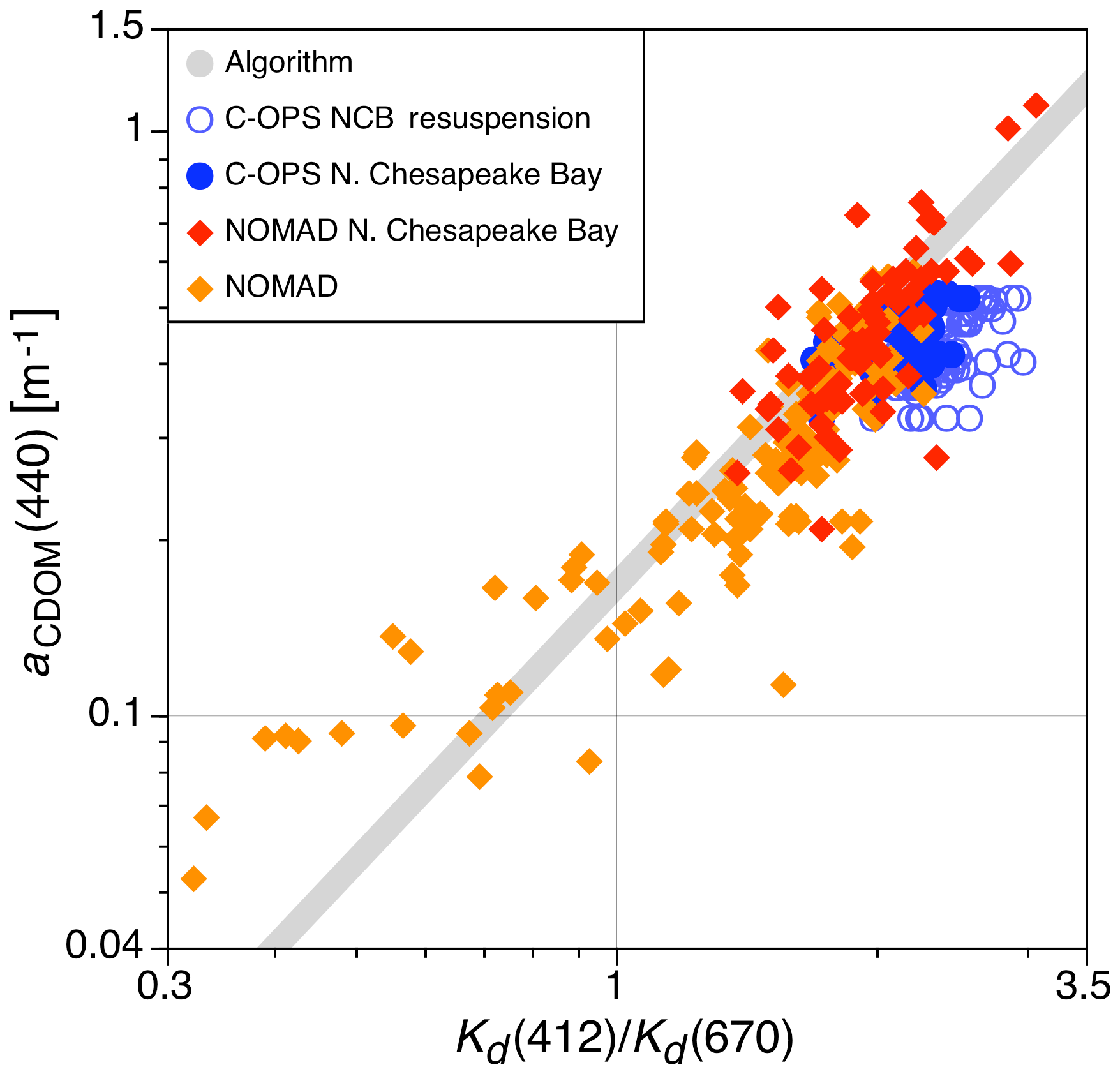
Figure 9The adherence of NOMAD archival data to the legacy (VIS) Kd(412)∕Kd(670) algorithm shown in Fig. 8 (gray solid circles) for the NCB and other Mid-Atlantic Bight locations (red and orange solid diamonds, respectively), recalling that only a linear perspective consistent with the relationship is considered herein. The NOMAD NCB data are compared to C-OPS NCB data obtained at different times and locations with the latter separated into two categories, wherein one is likely subjected to bottom resuspension (light blue open circles) and the other is not (dark blue solid circles).
The C-OPS and NOMAD data plotted in Fig. 9 show general agreement (linearity) of the NOMAD data with respect to the algorithm, which independently confirms the Hooker et al. (2013) algorithmic approach (and as evaluated in more detail herein). Within the narrower turbidity range of the NOMAD and C-OPS NCB data without likely resuspension, there is improved agreement. The C-OPS NCB resuspension data appear properly categorized because of their relationship to the algorithm (Fig. 5). There is evidence the C-OPS data considered free of resuspension effects nonetheless include some resuspension (e.g., some solid circles in Fig. 9 extend into the open circles as part of shallow-to-deep transects, thereby indicating the transect point in which resuspension effects were assumed absent was likely premature). The NOMAD data exhibit a higher variance with respect to the algorithm, which results in an increased RMSE of 37.8 % (or 44.1 % if the 13 omitted observations are included) compared to the 6.2 % value determined with C-OPS data (Fig. 8). The more extreme NOMAD values suggest a subcategorization methodology that could be applied to archival data would improve agreement with the algorithm (already demonstrated with the removal of 13 observations using the algorithm in Fig. 8).
If the NOMAD data are partitioned into turbid and clear subsets, using aCDOM(440)>0.2 and aCDOM(440)≤0.2 as thresholds, respectively, the fit equation for the turbid data is . The slope of this turbid NOMAD fit is similar to the corresponding end-member fit presented in Fig. 8 for which and agrees to within 1.9 %. The fit for the clear NOMAD data (which include the 13 stations which were removed out of the 225 NOMAD stations) is , which is significantly different at the 78.4 % level. With respect to the algorithm, the increased bias, variance, and 13 negative derived values obtained with NOMAD data in clearer waters suggest that the linear perspective for end-member analysis is challenged by the reduction in spectral distance between end-member pairs and that the legacy data are degraded by sampling artifacts, e.g., wave-focusing effects (because of the slower sampling rates), coarser VSR (because of faster descent rates), and deeper extrapolation intervals (because of near-surface data loss from large vertical tilts and large aperture depth offsets). Although some legacy data problems are absent from C-OPS data (e.g., because there is no righting moment when C-OPS sampling begins and C-PrOPS stabilizes the planar orientation of all apertures), some aspects of these limitations are present in the Fig. 8 data, but they are not significant; i.e., they result in a small increase in variance, which slightly degrades algorithm performance. Inclusion of the C-OPS NCB data without resuspension to derive the algorithm (Fig. 8) results in rather small changes to the fit coefficients. The slope is within 4.3 % and the intercept is within 4.6 % (both within the net 5 % uncertainty for calibration and environmental variance).
3.7 Objective versus subjective classification
The data set established herein has an extensive number of observations directly suitable for validation exercises (Figs. 3 and 9) plus 15 subcategories (Sect. 2.5) of more complex, and thus potentially (but not automatically) questionable, water bodies (Figs. 4–7), with the latter determined subjectively. The combination yields 16 categorizations of data spanning an arguably global sampling of open ocean, coastal zone, and inland water masses in terms of a generalized perspective of the dynamic range in water properties (Figs. 3–8). The NOMAD search (Sect. 3.6), however, showed archival data provided a significantly less global data set in terms of spectral expanse and dynamic range as used herein. Archival data usually do not include a subcategory parameter for the observations; e.g., NOMAD has no applicable keyword. Although some subcategories could be determined from geolocation, temporal, and survey information (e.g., a harbor, wetland, alkaline lake), other influences are not usually established without an observer (e.g., atypical bloom or resuspension caused by a vessel). Consequently, a subcategorization based on the optical measurements alone might be advantageous to the validation process, particularly for archival data.
The subcategory approach is evaluated using Kd(λ) spectra for the aforementioned 16 subcategories of data, which can be described objectively based on spectral shapes and magnitudes. A small number of observations are excluded to ensure consistency in the determination of all Kd(λ) values; e.g., the White Lake data had estimated values in the UV domain, Bear Lake is a unique scattering anomaly created by calcium carbonate particles, and ship-induced resuspension is anthropogenic in origin. With the additional restriction of wavelength commonality spanning 320–780 nm (Table 1), a total of 1171 spectra are used for the objective classification analysis.
Application of the FCM classification to log-transformed Kd(λ) data for the 16 subcategorizations successfully classifies all Kd(λ) spectra into five classes based on the Calinski and Harabasz (1974) index (Sect. 2.7). Spectral shapes, as well as their magnitudes, uniquely vary between the five classes and span a continuum of water masses from oceanic and lacustrine case-1 to extreme case-2 inland waters. The continuum of water mass composition is summarized by the centered spectra for the five FCM classes shown in Fig. 10, where Ni is the class number set by index i. The diversity achieved in sampling lacustrine water masses is revealed in Fig. 10 by the range of Kd(λ) spectra for the example drought-stricken and refilled lakes shown, which are compared with Crater Lake and Kw. The refilled lakes are shown to emphasize the complex relationships presented in Figs. 4–7 are not detectable by Kd(λ) alone, but require an understanding of the applicable end-member ratio and the aCDOM(440) value.
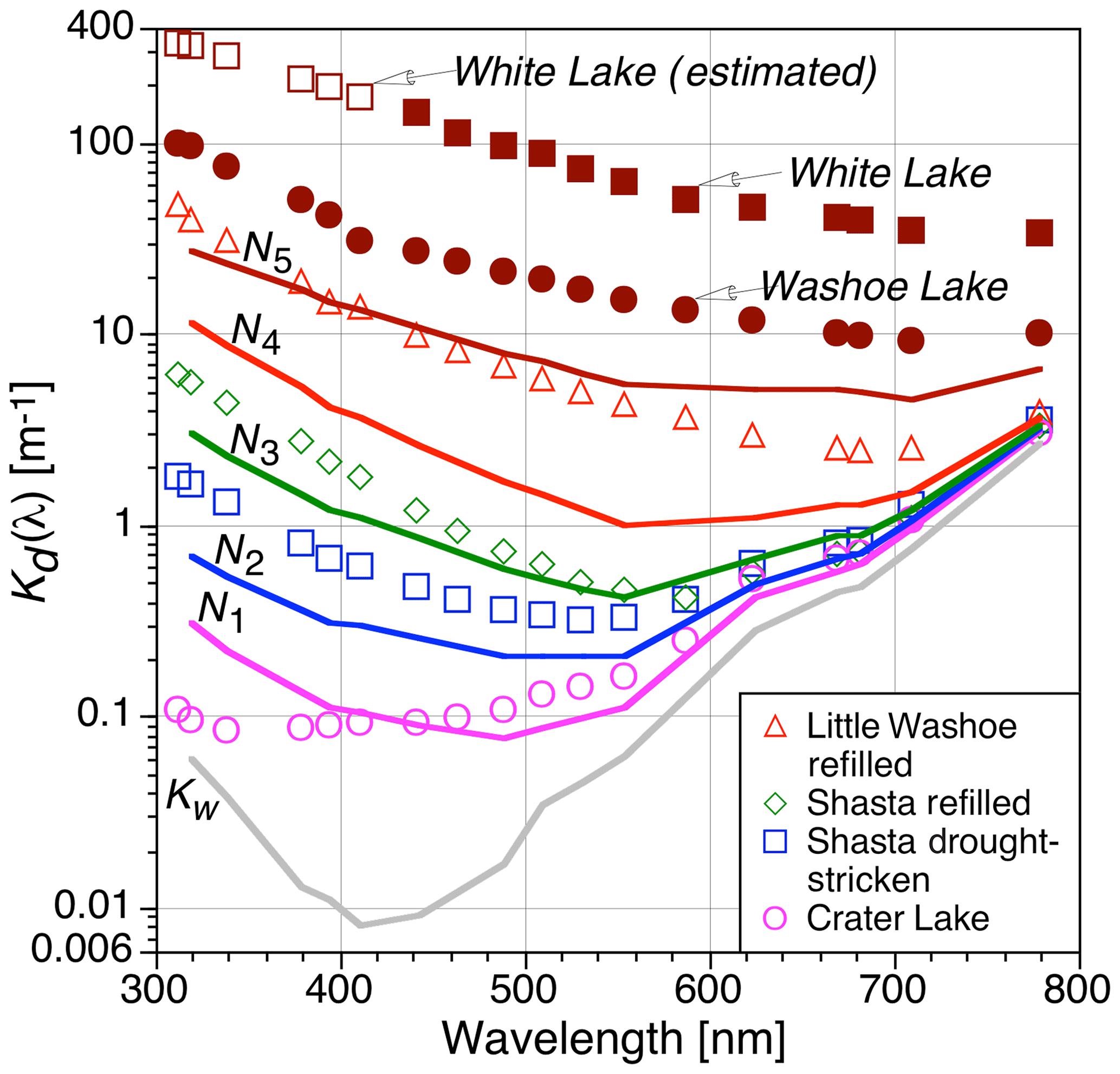
Figure 10The centered Kd(λ) spectra of the five classes (Ni) determined from an objective FCM classification of the data presented in Figs. 3–8 with a few omissions for data consistency (e.g., White Lake, Bear Lake, ship-induced resuspension) and shown with respect to Kw. Example Kd spectra from drought-stricken and refilled lakes plus Crater Lake, obtained by averaging the results from multiple optical casts, are also shown to demonstrate the more than 3 decades of dynamic range in turbidity that were sampled. The shorter wavelengths for White Lake (open dark red squares) required individual wavelength processing to provide the estimated Kd values, whereas all other data were obtained with a single processing.
The two lakes at the bottom and top of the dynamic range in Fig. 10 are Crater Lake and White Lake, respectively, with the latter having the largest displacement with respect to the algorithm in Figs. 4–7. Using the inverse of Kd(λ) as a proxy for the vertical scale that must be properly sampled (i.e., a sufficient number of observations must be obtained within the vertical scale to derive data products), the vertical scale in Fig. 10 ranges from meters (Crater Lake) to millimeters (White Lake), with the latter only being possible with unprecedented VSR. The shorter wavelengths for White Lake are shown as “estimated” because these wavelengths had to be processed with individual extrapolation intervals to provide the Kd(λ) estimates, which is not in keeping with all the other data products.
The average Kd(313) value obtained for deep water (586 m) sampling in Crater Lake was 0.072 m−1 and the coefficient of variation from the six casts was 1.1 %. According to Morel et al. (2007) criteria, Crater Lake is “extremely” clear water, and the CV shows exceptional reproducibility, i.e., 1 % radiometry. Note that as shown in Fig. 3, Crater Lake was sampled twice. A station with higher aCDOM(440) values was conducted in shallower water above submerged moss that grows in large, dense mats. The constituent properties of the water were anticipated to be influenced by the moss mats, and the aCDOM(440) values are elevated with respect to the deeper station.
Table 2The objective FCM classification of the data in Figs. 3–8 with a few omissions to ensure consistent data quality (e.g., White Lake, Bear Lake, ship-induced resuspension). The five classes Ni, where i is the class number index, are shown with the number of Kd(λ) spectra, Ns, within each class in parentheses, as well as the percent composition of the original 16 subjective subcategories equalling or exceeding a 1 % contribution threshold for each class. The principal subcategories in each class, i.e., the most numerous (approximately 5 % contribution or more), are shown in bold. Below the subcategories, the number of principal subcategories (Np) and the number of all subcategories (Na) with a 1 % composition or more are summarized in slanted typeface followed by the percent composition from all the principal subcategories. The extent of the dynamic range in percent for the optical and biogeochemical data is shown in the last two lines as a function of applying successive class numbers.
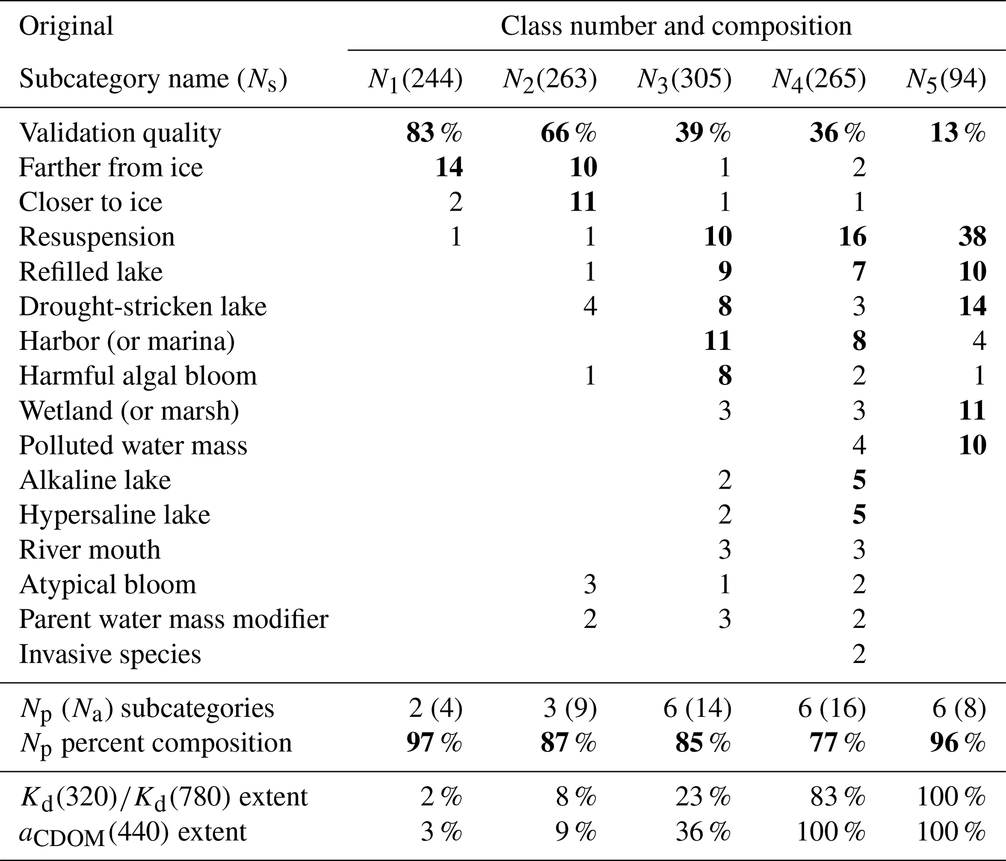
The proportionate composition of each FCM class in Fig. 10 as a function of the original subjective subcategories, wherein contributions less than 5 % are reported but not considered significant, is presented in Table 2. Using Fig. 10 and Table 2, the corresponding principal class characteristics are as follows.
- N1
-
The first is the smallest contributor to the dynamic ranges, although arguably accounting for most of the pixels in a global CDOM image, with the Kd(λ) maximum in the NIR and the minimum in the blue domain (400–490 nm). The spectral shape is consistent with typical case-1 waters (Morel and Maritorena, 2001). The proportional makeup is dominated by the validation quality subcategory (Figs. 3 and 8) at 83 % with data farther from ice (Fig. 5), which are almost exclusively from slightly modified case-1 waters, contributing an additional 14 %.
- N2
-
The Kd(λ) maximum in the NIR is similar to case-1 waters, and the minimum is shifted to longer wavelengths (490–565 nm) from case-1 modifications, principally from proximity to ice effects. The validation quality proportion decreases to 66 % and is supplanted with proximity to ice subcategories (Fig. 5).
- N3
-
The Kd(λ) minimum is near the middle of the green domain (555–565 nm) due to increasing optical complexity as case-2 constituents appear in larger proportions. The UV domain values are the same as, or slightly lower than, the NIR domain. The validation quality proportion decreases to 39 % while case-2 subcategories increase significantly, i.e., resuspension, drought-stricken and refilled lakes, harbors, and HABs.
- N4
-
The aCDOM(440) dynamic range is established with the Kd(λ) minimum shifted into the green–red domains (555–625 nm) and maximum values in the UV exceeding the NIR. Optical complexity reaches a maximum, because all 16 categorizations contribute at the 1 % level or more. The validation quality proportion is the most abundant but is decreased to 36 %. The resuspension, harbor, and refilled lake subcategories provide net increases in case-2 waters with additional extreme contributions from alkaline and hypersaline lakes.
- N5
-
The last are extreme waters that only extend the optical dynamic range, with the Kd(λ) minimum in the NIR domain (710 nm), and maximum values compared to N1–N4 that peak in the UV. The resuspension subcategory is dominant at 38 %, followed by drought-stricken lakes at 14 %, and the validation quality subcategory is reduced to 13 %. The remaining principal contributors are wetlands, refilled lakes, and polluted water bodies.
The decrease in the percent composition of the validation quality data as a function of increasing class number (N1–N5) is an indicator of the difficulty of validating an algorithm within increasingly complex waters. The recurring contribution of a relatively small number of principal subjective subcategories to the gradient in optical complexity confirms the subcategory approach has merit and reveals the cause-and-effect relationships of the subcategories.
Table 2 also indicates the resolution or granularity for the 15 subcategories of more complex water masses was more nuanced than required. For example, alkaline and hypersaline lakes could be one subcategory, as could refilled and drought-stricken lakes. Combining subcategories does not ensure an eventual convergence with the objective FCM classification, because the latter partitions the processes present in the subcategories into varying degrees of contribution for each identified class. This partitioning involves both direct and indirect evidence, which is perhaps best realized with the original granularity of the 15 subcategories as revealed by considering resuspension processes.
The direct evidence of resuspension is provided by the resuspension subcategory (created for this phenomenon). Indirect resuspension is present or likely in multiple subcategories, however. For example, meltwater releases particles at the ice edge, bottom deposits in harbors are stirred up by boat propellers, wind and rain redeposit exposed bottom material into drought-stricken lakes, refilled lakes contain suspended material from riverine inflow, and tidal and wave action suspend material in shallow wetlands. Table 2 data show the percent contribution of direct and indirect suspension increases with increasing class number: N1 (17 %) to N3 (46 %) to N5 (77 %). Thus a significant part of the cascade towards complexity is correlated with water masses not evolving conservatively, e.g., due to resuspension.
A small number of principal subcategories (Np) significantly determine the Kd(λ) classification spectra, although the paucity of observations for some subcategories, in part opportunistic or planned, depending on the subcategory, is a largely unknown mitigating factor. Nonetheless, if refilled and drought-stricken lakes plus hypersaline and alkaline lakes are considered one subcategory rather than two, which appears reasonable based on Fig. 4, five or fewer principal subcategories determine 97 %, 92 %, 85 %, 80 %, and 96 % of the composition for N1–N5, respectively.
Without the subcategory scheme, the importance of direct or indirect resuspension would not have emerged with the clarity provided in Table 2. The composition of the FCM classes confirms the applicability of subcategories while revealing which ones are important to each class and which ones are marginally or not important. For the latter, the parent water mass modifier is not significant, as expected, because this small subcategory was created to demonstrate the sensitivity of the in situ optical and laboratory methods. Other subcategories might appear insignificant because of the difficulty of obtaining the sample (e.g., river mouth data are underrepresented) or the paucity of opportunities to collect a sample (e.g., local restrictions to prevent the spread of invasive species).
Because metadata to subcategorize NOMAD data are unavailable, the objective classification scheme was applied to NOMAD and to determine the number of data in each class, as follows: N1 6, N2 13, N3 135, N4 49, N5 0, and nine were unclassified. All the turbid data are in classes N3 and N4; the clear data are in classes N1 and N2, and nine are unclassified. This means the slope of the aforementioned clear partition (Sect. 3.6) had 19 points that were classified and nine that were not, and this likely accounts for the degraded performance with respect to the algorithm. It also suggests the measurements were the issue with the NOMAD data, because some spectra could not be classified.
The optical data herein had a near-surface VSR less than 1 mm, which allowed data products spanning 313–875 nm while encompassing a global perspective of water masses as described by approximately 3 decades of generalized water properties. The validation approach was based on the concept that water masses evolving conservatively (i.e., free from stressors that might alter the natural range in the gradient of a constituent) are suitable for validating the original Hooker et al. (2013) inversion algorithm for deriving aCDOM(440) from Kd(λ) spectral end-members.
The identification of 15 subcategories that were likely not evolving conservatively yielded 609 validation quality data points spanning extremely clear to highly turbid waters sampled within the open ocean, coastal zone, and inland waters. The new data adhered to the original algorithm (Fig. 3) with an RPD of 0.02 % and an APD of 3.86 %. Alternative spectral end-members (e.g., , , and ) had increasingly larger RMSE values but were within the calibration uncertainty of the radiometers plus inevitable environmental variance (i.e., a net uncertainty within 5 %) except for the narrowest spectral span of legacy end-members, which was 6.2 % for (Fig. 8) due to increased variance in data products plus increasing algorithmic nonlinearity for spectrally closer end-members.
Although no archive exists with the spectral and spatial coverage used herein, NOMAD data showed general agreement (of derived coefficients) with respect to the original Hooker et al. (2013) algorithm and independently confirmed the algorithmic approach. There was also general agreement between the NOMAD NCB data and the corresponding C-OPS NCB data without likely resuspension, wherein the C-OPS NCB resuspension data appeared properly categorized because of their relationship with the algorithm (Fig. 5). The near-surface VSR is quantitative evidence of the successful mitigation of a variety of sampling difficulties (e.g., large aperture offsets, righting moment instabilities, wave-focusing effects). The C-OPS VSR resulted in an increased sampling sensitivity in turbid waters with vertical scales on the order of millimeters (Fig. 10) and allowed small localized changes in a parent water mass to be distinguished (Figs. 5 and 7). The laboratory analyses were similarly sensitive, so the optical determinations of in-water constituents using field measurements were commensurately as effective as laboratory analyses. The ability to distinguish small differences in water properties ensured the discrimination of 15 subcategories, wherein each represented a more complex water mass not evolving conservatively and not automatically used for validation.
Plots of the aCDOM(440) and relationships for the 15 subcategories of more complex water bodies revealed some data were significantly different with respect to the original algorithm and others were not (Figs. 4–7). The wide range in complexity is largely the result of the substantial effort that was made to adopt a global perspective and sample the greatest diversity of water bodies possible, some of which were very difficult to access and sometimes required shoreline launches of the optical instrumentation that C-PrOPS made possible, e.g., severely drought-stricken and refilled lakes (high and dry, flooded, or debris-blocked boat ramps) plus hypersaline and soda lakes (Mono Lake, Salton Sea, Borax Lake, and Soda Lake had no boat ramps).
The accuracy of the algorithm as a function of including increasing proportions of the 15 subcategories of more complex water masses not necessarily appropriate for validation exercises (Figs. 4–7), because they were likely not evolving conservatively, is explored by expanding the 609 validation quality observations of end-members (Figs. 3 and 8) to include the following subcategories (hereafter referred to as the second data set): inflows to a parent water mass that are not hypersaline or drought-stricken lakes, closer to or farther from ice edge proximity, river mouth, resuspension (but not including Bear Lake and the ship-induced RWC channel resuspension), atypical blooms, HABs, and wetlands. This second data set has 930 observations, the linear fit is , the RMSE is 5.7 %, and the new slope is within 1.7 % of the original value presented by Hooker et al. (2013), i.e., .
The reason the slope for the second data set is not significantly different than the original fit coefficients is the data that were added are situated above and below the distribution of the validation quality data set, as shown in Figs. 4 and 5. The C-OPS NCB data without resuspension cluster on or below the algorithmic relationship (Fig. 9). If these data are added to the second data set used to derive the algorithm (the 320 and 780 nm wavelengths were always part of system 021 as shown in Table 1), the resulting slope and intercept is , which is within 2.0 % of the slope determined for the second data set ().
If a third data set is created by adding drought-stricken and refilled lakes to the second data set, but not including White Lake (which had some estimated data products), this third data set has 1044 observations. The linear fit is , the RMSE is 6.8 %, and the new slope is reduced (as expected, because the added data are all below the algorithmic relationship and primarily turbid; Fig. 4), but still within 10.4 % of the original value presented by Hooker et al. (2013). The exclusion of White Lake, as well as hypersaline, alkaline, and polluted water bodies, from the third data set is for a practical reason: they are, or have significant characteristics of, extreme water masses and White Lake rarely exists.
There are other lacustrine water bodies presented herein that can be considered extreme, e.g., other endorheic lakes (e.g., Pyramid Lake, Eagle Lake), plus shallow lakes in high wind areas wherein bottom material is resuspended almost continuously (e.g., Washoe Lake and Little Washoe Lake). If all subcategories, except extreme lacustrine water bodies, are used to create a fourth data set, it has 1086 observations, i.e., almost 90 % of the 1230 maximum and 93 % of the data used in Table 2 to create the five objective FCM classifications. The linear fit of this fourth, more comprehensive data set is , the RMSE is 6.2 %, and the new slope is not reduced as much as in the third data set and is within 6.9 % of the original value presented by Hooker et al. (2013).
A fifth data set, using classes N1–N4 spans the entire aCDOM(440) dynamic range (Table 2). This alternative for an arguably global algorithm yields a linear fit of ; the RMSE is 5.3 %, and the slope is within 9.3 % of the original Hooker et al. (2013) value. This result is significantly similar to the subjective results of the fourth data set (the slopes agree within 2.7 %). Consequently, the robustness of the algorithm is directly supported by the combination of subjective and objective classifications, with the latter using FCM.
With the exception of the third data set that added primarily turbid data exclusively below the algorithmic relationship (drought-stricken and refilled lakes), all of the results from the expanded data sets are rather indistinguishable from the original fit provided by Hooker et al. (2013), wherein , or the separate validation quality data set presented in Fig. 8, for which . Ignoring the third data set, the x intercept for the expanded data sets is approximately equal to what can be expected for pure water, i.e., 0.02. The close agreement of the various expanded data sets with adherence to the pure-water limit is another significant confirmation of the algorithmic approach using spectral end-members.
The robustness is further established by creating a so-called universal algorithm, which is assumed to mean that any water mass wherein an optical profiler can be deployed is expected to be part of the evaluation of the end-member approach. In this case, the universal algorithm is constructed from all the data from all subcategories and is distinguished from the global perspective in that the universal data set includes a far greater proportion of complex water types than exist globally. The linear fit of this universal data set is , the RMSE is 7.5 %, and the new slope is within 13.7 % of the original value presented by Hooker et al. (2013). The removal of data that are, or have significant characteristics of, extreme water masses improves performance. For example, if hypersaline, alkaline, and polluted lakes are removed, the linear fit of this sixth comprehensive data set is , the RMSE is 6.8 %, and the new slope is within 12.0 % of the original value presented by Hooker et al. (2013).
This study used three different laboratory methods to determine aCDOM(440) from water samples and seven different optical instrument suites to determine Kd(λ). Despite the agreement between the fits and their x intercepts, the possibility the results come from an unidentified stochastic process has not been addressed. The latter is not likely for the optical data, because the radiometers were calibrated at one facility and deployed with strict adherence to the protocols using the same acquisition software. Furthermore, data products were derived using the same processing software with one operator, and the variance in optical data products is shown in Figs. 3–8.
The capabilities of the above- and in-water radiometers for C-OPS systems 021 (with C-PrOPS) and 039 (without C-PrOPS) were intercompared to next-generation hybrid-spectral instruments (Hooker et al., 2018c) containing a hyperspectral detector system plus 18 fixed wavelengths (system 038 in Table 1). The comparisons showed an agreement of 4.2 %–4.8 %, which is within the calibration uncertainty (2.3 %–2.7 %) plus natural variability (i.e., a net uncertainty within 5 %), as long as the stability threshold for a backplane without thrusters or the noise limit of the hyperspectral sensor was not exceeded (Hooker et al., 2018b, c).
Although field data demonstrate small changes in parent water mass modifications can be discriminated (Figs. 5 and 7), the laboratory methods and instruments were not systematically intercalibrated to establish an overall uncertainty. In addition, the laboratory methods included different temperature controls and storage procedures for the water samples as well as application of null-point corrections in different spectral ranges. A lack of systematic intercalibration is not a significant detraction, because it is a common difficulty when combining observations from databases (e.g., NOMAD data), and methods exist to nonetheless determine the efficacy of the combined data.
Following the technique established by Matsuoka et al. (2017), a statistical sensitivity analysis is used to examine the uncertainty of the combined aCDOM(440) values from the three different laboratory methods used in Figs. 3–8. Briefly, for each optical and water sampling, normality of distribution for aCDOM(440) was created using the measured value as the mean (μ) and 7 % of the measured value as the standard deviation (σ). Similarly, normality of distribution for was created using the measured value as μ and 5 % as σ. A lower σ percentage was used for the latter, because the original data set retained each optical cast whereas only one water sample was obtained, so the variability of the optical data was already significantly represented (Figs. 3–8).
For each original data pair, 105 variations were prepared for both and aCDOM(440). Of these data, 103 were randomly selected and the mean computed for each and aCDOM(440) pair. This exercise was repeated 103 times (bootstrap) and an overall μ and σ were obtained. For the different combinations of applying μ±σ to bound the dispersion of the original data, the resulting linear fits showed the new algorithm slopes changed by 0.3 %–1.1 % with respect to the validation quality data set in Fig. 8. For all combinations of μ±σ, the maximum RMSE was 1.1 %, which is similar to the 1.2 % value for in Fig. 8. Consequently, the use of three different laboratory methods to determine aCDOM(440), which was not intercalibrated, does not significantly influence the results presented here.
The state-of-the-art (approximately 1 %) accuracy achieved with the end-members (Fig. 8) is, therefore, due to the strict adherence to sampling and processing protocols coupled with an unprecedented VSR of the optical data. This combination also resulted in all end-member pairs – including the legacy (VIS) pair – having a superior accuracy compared to many common global inversion algorithms. For example, aCDOM(λ) algorithms based on the water-leaving radiance, LW(λ), and its normalized forms have an RMSE exceeding 10 % or more (Mannino et al., 2008, 2014), and the ocean color (OC) chlorophyll a variants that use band ratios (O'Reilly et al., 1998, 2000) typically exceed 20 % or more while generally excluding complex and inland waters as used herein.
The robustness of the end-member approach is further confirmed by how the expanded data sets (up to six), which had increased amounts of optically complex water masses that were not evolving conservatively, nonetheless yielded fits with RMSE values outperforming the aforementioned LW(λ) algorithms. With regards to which of the variants best represents a global perspective, the pairs in Fig. 8 are considered appropriate. Screening of newly collected or archival data, e.g., NOMAD data (Sect. 3.7), with respect to a selected algorithm can be accomplished by initially flagging data points more than 12 % from the expected relationship and then more carefully examining those points using both objective and subjective criteria (based on available metadata) to determine whether the results are expected or are more likely to indicate a problem with data collection procedures.
If an algorithm is to be applied to a water mass that is not evolving conservatively, an individualized relationship between aCDOM(λ) and should be established, especially for an extreme water mass, e.g., drought-stricken. This maintains the accuracy of the global relationship while providing a mechanism for improving the study of nonconservative waters. Identification of water masses not evolving conservatively can likely be determined using Kd(λ) values determined from in-water optical (e.g, C-OPS) data without a need for laboratory analyses (Fig. 9). With additional research to produce Kd(λ) for all wavelengths, e.g., expanding upon Cao et al. (2014), the identification of water masses evolving conservatively or not can be made from above-water observations. This determination provides a sensitive indicator of water masses subjected to stresses influencing water quality, e.g., drought. The onset of next-generation satellites, e.g., the Japanese Second-generation Global Imager (SGLI) mission (Honda et al., 2012), offers unique opportunities for such monitoring because of the expanded spatial and spectral domain, with the latter allowing improved algorithm accuracy with respect to legacy missions, e.g., Moderate Resolution Imaging Spectroradiometer (MODIS). While planned high-spectral-resolution sensors, such as the Plankton, Aerosol, Cloud, ocean Ecosystem (PACE) and Surface Biology and Geology (SBG) missions, may support more sophisticated retrievals of parameters like CDOM, the simplified approach provided by end-member analysis can be used with both legacy and next-generation sensors, thereby providing continuity in space and time as well as a capability to generate high-quality in-water data with a simplified measurement approach (assuming strict adherence to the protocols).
The underlying research data presented in this study are available from the first corresponding author by request.
Conceptualization of the study was done by SBH, AM, and RMK; the methodology was established by SBH, AM, RMK, YY, and HFH; the software was implemented by SBH and AM; validation was done by SBH, AM, RMK, and HFH; formal analysis of the data was done by SBH, AM, RMK, and HFH; the investigation of hypotheses was done by SBH, AM, RMK, YY, KS, and HFH; resources were obtained by SBH, AM, RMK, and KS; data collection was obtained by SBH, AM, RMK, YY, KS, and HFH; the original draft was prepared by SBH, AM, RMK, YY, and HFH; review and editing was done by SBH, AM, RMK, YY, KS, and HFH; visualization of the results was done by SBH, AM, RMK, and HFH; supervision of the study was done by SBH, AM, and RMK; project administration was done by SBH, AM, RMK, YY, and KS; funding acquisition was done by SBH, AM, RMK, YY, and KS.
The authors declare that they have no conflict of interest.
This work was principally supported by the National Aeronautics and Space Administration (NASA) as part of planning for the Aerosol, Cloud, Ecosystems (ACE) satellite remote sensing mission. The next-generation perspective benefitted from the anticipated calibration and validation activities of the SGLI, ACE, and PACE missions. The high level of success achieved in the fieldwork established a foundation of understanding that was the direct consequence of contributions from individuals who contributed unselfishly to the work involved (e.g., calibration, acquisition, processing, and sampling). The scientists included (alphabetically) James Brown, Bruce Hargreaves, Toru Hirawake, Tomonori Isada, Randall Lind, John Morrow, Kendra Negrey, and Jun Nishioka; their dedicated contributions are gratefully acknowledged.
This research has been supported by the NASA ACE Mission Office. Additional field sampling opportunities were provided by the following NASA projects: Hyperspectral Infrared Imager (HyspIRI), Coastal and Ocean Airborne Science Testbed (COAST), Coastal High Acquisition Rate Radiometers for Innovative Environmental Research (C-HARRIER), and Hybridspectral Alternative for Remote Profiling of Optical Observations for NASA Satellites (HARPOONS). Part of this study was supported by the Japan Aerospace Exploration Agency (JAXA) Global Change Observation Mission-Climate (GCOM-C) project to A. Matsuoka (principal investigator ER2GCF310).
This paper was edited by Maria Tzortziou and reviewed by two anonymous referees.
Antoine, D., Hooker, S. B., Bélanger, S., Matsuoka, A., and Babin, M.: Apparent optical properties of the Canadian Beaufort Sea – Part 1: Observational overview and water column relationships, Biogeosciences, 10, 4493–4509, https://doi.org/10.5194/bg-10-4493-2013, 2013.
Aurin, D., Mannino, A., and Lary, D. J.: Remote Sensing of CDOM, CDOM Spectral Slope, and Dissolved Organic Carbon in the Global Ocean, Appl. Sci., 8, 2687, https://doi.org/10.3390/app8122687, 2018.
Bierly, K., Burgess, P., Fetcho, K., Gregory, S., Graham-Hudson, B., Hudson, W., Hulse, D., Moore, K., Mullan, A., Wallick, R., Welch, D., and Wiley, P.: Tracking Progress in Restoring the Willamette River Floodplain, Habitat Technical Team Pub., Oregon Department of Fish and Wildlife, Salem, Oregon, 13 pp., 2015.
Bodaker, I., Sharon, I., Suzuki, M. T., Feingersch, R., Shmoish, M., Andreishcheva, E., Sogin, M. L., Rosenberg, M., Maguire, M. E., Belkin, S., and Oren, A.: Comparative community genomics in the Dead Sea: an increasingly extreme environment, ISME J., 4, 399–407, 2010.
Bushaw, K. L., Zepp, R. G., Tarr, M. A., Schultz-Jander, D., Bourbonniere, R. A., Hodson, R. E., Miller, W. L., Bronk, D. A., and Moran, M. A.: Photochemical release of biologically available nitrogen from aquatic dissolved organic matter, Nature, 381, 404–407, 1996.
Calinski, T. and Harabasz, J.: A dendrite method for cluster analysis, Commun. Stat., 3, 1–27, 1974.
Cao, F., Fichot, C. G., Hooker, S. B., and Miller, W. L.: Improved algorithms for accurate retrieval of UV/visible diffuse attenuation coefficients in optically complex, inshore waters, Remote Sens. Environ., 144, 11–27, 2014.
Davis, J. and Milligan, M.: Why is Bear Lake so Blue? And Other Commonly Asked Questions, Public Information Series 96, Utah Geological Survey, Salt Lake City, Utah, 42 pp., 2011.
Fellman, J. B., D'Amore, D. V., and Hood, E.: An evaluation of freezing as a preservation technique for analyzing dissolved organic C, N and P in surface water samples, Sci. Total Environ., 392, 305–312, 2008.
Gordon, H.R., and Ding, K.: Self shading of in-water optical instruments Limnol. Oceanogr., 37, 491–500, 1992.
Grant, W. D.: Extremophilies – Alkaline Environments and Biodiversity, in: Encyclopedia of Life Support Systems (EOLSS), edited by: Gerday, C. and Glansdorff, N., Eolss Publishers, Oxford, United Kingdom, 20 pp., 2006.
Green, S. A. and Blough, N. V.: Optical absorption and fluorescence properties of chromophoric dissolved organic matter in natural waters, Limnol. Oceanogr., 39, 1903–1916, 1994.
Grunert, B. K., Mouw, C. B., and Ciochetto, A. B.: Characterizing CDOM spectral variability across diverse regions and spectral ranges, Global Biogeochem. Cy., 32, 57–77, 2018.
Guarch-Ribot, A. and Butturini, A.: Hydrological conditions regulate dissolved organic matter quality in an intermittent headwater stream. From drought to storm analysis, Sci. Total Environ., 571, 1358–1369, 2016.
Heisler, J., Glibert, P., Burkholder, J., Anderson, D., Cochlan, W., Dennison, W., Gobler, C., Dortch, Q., Heil, C., Humphries, E., Lewitus, A., Magnien, R., Marshall, H., Sellner, K., Stockwell, D., Stoecker, D., and Suddleson, M.: Eutrophication and harmful algal blooms: A scientific consensus, Harmful Algae, 8, 3–13, 2008.
Hancke, K., Hovland, E. K., Volent, Z., Pettersen R., Johnsen G., Moline M., and Sakshaug E.: Optical properties of CDOM across the Polar Front in the Barents Sea: Origin, distribution and significance, J. Mar. Sys., 130, 219–227, 2014.
Honda, Y., Kajiwara, K., Sharma, R., Ono, A., Imaoka, K., Murakami, H., Hori, M., Ono, Y., and Rostand, D.: Overview of GCOM-C1/SGLI science, Proc. SPIE, 8528, https://doi.org/10.1117/12.977772, 2012.
Hooker, S. B.: Mobilization Protocols for Hybrid Sensors for Environmental AOP Sampling (HySEAS) Observations, NASA Tech. Pub. 2014–217518, NASA Goddard Space Flight Center, Greenbelt, Maryland, 105 pp., 2014.
Hooker, S. B. and Esaias, W. E.: An overview of the SeaWiFS project, Eos, Trans. Amer. Geophys. Union, 74, 241–246, 1993.
Hooker, S. B., McClain, C. R., Firestone, J. K., Westphal, T. L., Yeh, E.-N., and Ge, Y.: The SeaWiFS Bio-Optical Archive and Storage System (SeaBASS), Part 1, NASA Tech. Memo. 104566, Vol. 20, edited by: Hooker, S. B. and Firestone, E. R., NASA Goddard Space Flight Center, Greenbelt, Maryland, 40 pp., 1994.
Hooker, S. B., Zibordi, G., Berthon, J.-F., D'Alimonte, D., Maritorena, S., McLean, S., and Sildam, J.: Results of the Second SeaWiFS Data Analysis Round Robin, March 2000 (DARR-00), NASA Tech. Memo. 2001–206892, Vol. 15, edited by: Hooker, S. B. and Firestone, E. R., NASA Goddard Space Flight Center, Greenbelt, Maryland, 71 pp., 2001.
Hooker, S. B., Morrow, J. H., and Matsuoka, A.: Apparent optical properties of the Canadian Beaufort Sea – Part 2: The 1 % and 1 cm perspective in deriving and validating AOP data products, Biogeosciences, 10, 4511–4527, https://doi.org/10.5194/bg-10-4511-2013, 2013.
Hooker, S. B., Lind, R. N., Morrow, J. H., Brown, J. W., Suzuki, K., Houskeeper, H. F., Hirawake, T., and Maúre, E. R.: Advances in Above- and In-Water Radiometry, Vol. 1: Enhanced Legacy and State-of-the-Art Instrument Suites, NASA Tech. Pub. 2018-219033, Vol. 1, NASA Goddard Space Flight Center, Greenbelt, Maryland, 60 pp., 2018a.
Hooker, S. B., Lind, R. N., Morrow, J. H., Brown, J. W., Kudela, R. M., Houskeeper, H. F., and Suzuki, K.: Advances in Above- and In-Water Radiometry, Vol. 2: Autonomous Atmospheric and Oceanic Observing Systems, NASA Tech. Pub. 2018-219033, Vol. 2, NASA Goddard Space Flight Center, Greenbelt, Maryland, 69 pp., 2018b.
Hooker, S. B., Lind, R. N., Morrow, J. H., Brown, J. W., Kudela, R. M., Houskeeper, H. F., and Suzuki, K.: Advances in Above- and In-Water Radiometry, Vol. 3: Hybridspectral Next-Generation Optical Instruments, NASA Tech. Pub. 2018-219033, Vol. 3, NASA Goddard Space Flight Center, Greenbelt, Maryland, 39 pp., 2018c.
Houser, J. N.: Water color affects the stratification, surface temperature, heat content, and mean epilimnetic irradiance of small lakes, Can. J. Fish. Aquat. Sci., 63, 2447–2455, 2006.
Jessup, D. A., Miller, M. A., Ryan, J. P., Nevins, H. M., Kerkering, H. A., Mekebri, A., Crane, D. B., Johnson, T. A., and Kudela, R. M.: Mass stranding of marine birds caused by a surfactant-producing red tide, PLoS One, 4, e4550, https://doi.org/10.1371/journal.pone.0004550, 2009.
Kudela, R. M., Palacios, S. L., Austerberry, D. C., Accorsi, E. K., Guild, L. S., and Torres-Perez, J.: Application of hyperspectral remote sensing to cyanobacterial blooms in inland waters, Remote Sens. Environ., 167, 196–205, 2015.
Kutser, T., Verpoorter, C., Paavel, B., and Tranvik, L.J.: Estimating lake carbon fractions from remote sensing data, Remote Sens. Environ., 157, 138–146, 2015.
Kwon, H. K., Kim, G., Lim, W. A., and Park, J. W.: In-situ production of humic-like fluorescent dissolved organic matter during Cochlodinium polykrikoides blooms, Estuar. Coast. Shelf Sci., 203, 119–126, 2018.
Lee, Z. and Hu, C.: Global distribution of Case-1 waters: An analysis from SeaWiFS measurements, Remote Sens. Environ., 101, 270–276, 2006.
Mannino, A., Russ, M. E., and Hooker, S. B.: Algorithm development and validation for satellite-derived distributions of DOC and CDOM in the U.S. Middle Atlantic Bight, J. Geophys. Res., 113, C07051, https://doi.org/10.1029/2007JC004493, 2008.
Mannino, A., Novak, M., Hooker, S. B., Hyde, K., and Aurin, D.: Algorithm development and validation of CDOM properties for estuarine and continental shelf waters along the northeastern US coast, Remote Sens. Environ., 152, 576–602, 2014.
Matsuoka, A., Bricaud, A., Benner, R., Para, J., Sempéré, R., Prieur, L., Bélanger, S., and Babin, M.: Tracing the transport of colored dissolved organic matter in water masses of the Southern Beaufort Sea: relationship with hydrographic characteristics, Biogeosciences, 9, 925–940, https://doi.org/10.5194/bg-9-925-2012, 2012.
Matsuoka, A., Hooker, S. B., Bricaud, A., Gentili, B., and Babin, M.: Estimating absorption coefficients of colored dissolved organic matter (CDOM) using a semi-analytical algorithm for southern Beaufort Sea waters: application to deriving concentrations of dissolved organic carbon from space, Biogeosciences, 10, 917–927, https://doi.org/10.5194/bg-10-917-2013, 2013.
Matsuoka, A., Babin, M., Doxaran, D., Hooker, S. B., Mitchell, B. G., Bélanger, S., and Bricaud, A.: A synthesis of light absorption properties of the Arctic Ocean: application to semianalytical estimates of dissolved organic carbon concentrations from space, Biogeosciences, 11, 3131–3147, https://doi.org/10.5194/bg-11-3131-2014, 2014.
Matsuoka, A., Boss, E., Babin, M., Boss, L.-K., Hafez, M., Chekalyuk, A., Proctor, C. W., Werdell, J., and Bricaud, A.: Pan-Arctic optical characteristics of colored dissolved organic matter: Tracing dissolved organic carbon in changing Arctic waters using satellite ocean color data, Remote Sens. Environ., 200, 89–101, 2017.
Moore, T. S., Campbell, J. W., and Feng, H.: A fuzzy logic classification scheme for selecting and blending satellite ocean color algorithms, IEEE Trans. Geosci. Remote Sens., 39, 1764–1776, 2001.
Moore, T. S., Campbell, J. W., and Feng, H.: Characterizing the uncertainties in spectral remote sensing reflectance for SeaWiFS and MODIS-Aqua based on global in situ matchup data sets, Remote Sens. Environ., 159, 14–27, 2015.
Mopper, K., Zhou, X., Kieber, R. J., Kieber, D. J., Sikorski, R. J., and Jones, R. D.: Photochemical degradation of dissolved organic carbon and its impact on the oceanic carbon cycles, Nature, 353, 60–62, 1991.
Morel, A.: Optical Properties of Pure Water and Pure Sea Water, in: Optical Aspects of Oceanography, edited by: Jerlov, N. G. and Nielsen, E. S., Academic Press, New York, 1–24, 1974
Morel, A. and Maritorena, S.: Bio-optical properties of oceanic waters: a reappraisal, J. Geophys. Res., 106, 7163–7180, 2001.
Morel, A., Gentili, B., Claustre, H., Babin, M., Bricaud, A., Ras, J., and Tièche, F.: Optical properties of the “clearest” natural waters, Limnol. Oceanogr., 52, 217–229, 2007.
Morrow, J. H., Hooker, S. B., Booth, C. R., Bernhard, G., Lind, R. N., and Brown, J. W.: Advances in Measuring the Apparent Optical Properties (AOPs) of Optically Complex Waters, NASA Tech. Memo. 2010–215856, NASA Goddard Space Flight Center, Greenbelt, Maryland, 80 pp., 2010.
Mouw, C. B., Greb, S., Aurin, D., DiGiacomo, P. M., Lee, Z., Twardowski, M., Binding, C., Hu, C., Ma, R., Moore, T., and Moses, W.: Aquatic color radiometry remote sensing of coastal and inland waters: Challenges and recommendations for future satellite missions, Remote Sens. Environ., 160, 15–30, 2015.
Mueller, J. L.: Overview of Measurement and Data Analysis Protocols, in: Ocean Optics Protocols for Satellite Ocean Color Sensor Validation, edited by: Fargion, G. S. and Mueller, J. L., Revision 2, NASA Tech. Memo. 2000–209966, NASA Goddard Space Flight Center, Greenbelt, Maryland, 87–97, 2000.
Mueller, J. L.: Overview of Measurement and Data Analysis Protocols, in: Ocean Optics Protocols for Satellite Ocean Color Sensor Validation, edited by: Mueller, J. L. and Fargion, G. S., Revision 3, Volume 1. NASA Tech. Memo. 2002–210004/Rev3–Vol1, NASA Goddard Space Flight Center, Greenbelt, Maryland, 123–137, 2002.
Mueller, J. L.: Overview of Measurement and Data Analysis Methods, in: Ocean Optics Protocols for Satellite Ocean Color Sensor Validation, edited by: Mueller, J. L., Fargion, G. S., and McClain, C. R., Revision 4, Volume III: Radiometric Measurements and Data Analysis Protocols, NASA Tech. Memo. 2003–211621/Rev4–Vol.III, NASA Goddard Space Flight Center, Greenbelt, Maryland, 1–20, 2003.
Mueller, J. L. and Austin, R. W.: Ocean Optics Protocols for SeaWiFS Validation, NASA Tech. Memo. 104566, Vol. 5, edited by: Hooker, S. B. and Firestone, E. R., NASA Goddard Space Flight Center, Greenbelt, Maryland, 43 pp., 1992.
Mueller, J. L. and Austin, R. W.: Ocean Optics Protocols for SeaWiFS Validation, Revision 1, NASA Tech. Memo. 104566, Vol. 25, edited by: Hooker, S. B., Firestone, E. R., and Acker, J. G., NASA Goddard Space Flight Center, Greenbelt, Maryland, 66 pp., 1995.
Nelson, N. B. and Siegel, D. A.: The global distribution and dynamics of chromophoric dissolved organic matter, Annu. Rev. Mar. Sci., 5, 447–476, 2013.
Nelson, N. B., Siegel, D. A., Carlson, C. A., Swan, C. M., Smethie Jr., W. M., and Khatiwala, S.: Hydrography of chromophoric dissolved organic matter in the North Atlantic, Deep-Sea Res. I, 54, 710–731, 2007.
O'Reilly, J. E., Maritorena, S., Mitchell, B. G., Siegel, D. A., Carder, K. L., Garver, S. A., Kahru, M., and McClain, C.: Ocean Color chlorophyll algorithms for SeaWiFS, J. Geophys. Res., 103, 24937–24953, 1998.
O'Reilly, J. E., Maritorena, S., O'Brien, M. C., Siegel, D. A., Toole, D., Menzies, D., Smith, R. C., Mueller, J. L., Mitchell, B. G., Kahru, M., Chavez, F. P., Strutton, P., Cota, G. F., Hooker, S. B., McClain, C. R., Carder, K. L., Müller-Karger, F., Harding, L., Magnuson, A., Phinney, D., Moore, G. F., Aiken, J., Arrigo, K. R., Letelier, R., and Culver, M.: SeaWiFS Postlaunch Calibration and Validation Analyses, Part 3, NASA Tech. Memo. 2000–206892, Vol. 11, edited by: Hooker, S. B. and Firestone, E. R., NASA Goddard Space Flight Center, Greenbelt, Maryland, 9–23, 2000.
Palmer, S. C., Kutser, T., and Hunter, P. D.: Remote sensing of inland waters: challenges, progress and future directions, Remote Sens. Environ., 157, 1–8, 2015.
Röttgers, R. and Doerffer, R.: Measurements of optical absorption by chromophoric dissolved organic matter using a point-source integrating-cavity absorption meter, Limnol. Oceanogr.-Method., 5, 126–135, 2007.
Smith, R. C. and Baker, K. S.: The analysis of ocean optical data, Ocean Optics VII, edited by: Blizard, M., SPIE, 478, 119–126, 1984.
Tanaka, K., Takesue, N., Nishioka, J., Kondo, Y., Ooki, A., Kuma, K., Hirawake, T., and Yamashita, Y.: The conservative behavior of dissolved organic carbon in surface waters of the southern Chukchi Sea, Arctic Ocean, during early summer, Sci. Rep., 6, 34123, https://doi.org/10.1038/srep34123, 2016.
Twardowski, M. S., Boss, E., Sullivan, J. M., and Donaghay, P. L.: Modeling the spectral shape of absorption by chromophoric dissolved organic matter, Mar. Chem., 89, 69–88, 2004.
Vazquez, E., Amalfitano, S., Fazi, S., and Butturini, A.: Dissolved organic matter composition in a fragmented Mediterranean fluvial system under severe drought conditions, Biogeochemistry, 102, 59–72, 2011.
Werdell, P. J. and Bailey, S. W.: An improved in-situ bio-optical data set for ocean color algorithm development and satellite data product validation, Remote Sens. Environ., 98, 122–140, 2005.
Yamashita, Y. and Tanoue, E.: Basin scale distribution of chromophoric dissolved organic matter in the Pacific Ocean, Limnol. Oceanogr., 54, 598–609, 2009.
Yamashita, Y., Nosaka, Y., Suzuki, K., Ogawa, H., Takahashi, K., and Saito, H.: Photobleaching as a factor controlling spectral characteristics of chromophoric dissolved organic matter in open ocean, Biogeosciences, 10, 7207–7217, https://doi.org/10.5194/bg-10-7207-2013, 2013.
Yapiyev, V., Sagintayev, Z., Inglezakis, V., Samarkhanov, K., and Verhoef, A.: Essentials of endorheic basins and lakes: A review in the context of current and future water resource management and mitigation activities in Central Asia, Water, 9, 798–819, 2017.
Zaneveld, J. R. V., Boss, E., and Barnard, A.: Influence of surface waves on measured and modeled irradiance profiles, Appl. Opt., 40, 1442–1449, 2001.
nonconservativewater masses. The influence of subcategories was confirmed with an objective cluster analysis.