the Creative Commons Attribution 4.0 License.
the Creative Commons Attribution 4.0 License.
 | 18 Feb 2020
Influence of oceanic conditions in the energy transfer efficiency estimation of a micronekton model
Audrey Delpech
Anna Conchon
Olivier Titaud
Patrick Lehodey
Micronekton – small marine pelagic organisms around 1–10 cm in size – are a key component of the ocean ecosystem, as they constitute the main source of forage for all larger predators. Moreover, the mesopelagic component of micronekton that undergoes diel vertical migration (DVM) likely plays a key role in the transfer and storage of CO2 in the deep ocean: this is known as the “biological pump”. SEAPODYM-MTL is a spatially explicit dynamical model of micronekton. It simulates six functional groups of vertically migrant (DVM) and nonmigrant (no DVM) micronekton, in the epipelagic and mesopelagic layers. Coefficients of energy transfer efficiency between primary production and each group are unknown, but they are essential as they control the production of micronekton biomass. Since these coefficients are not directly measurable, a data assimilation method is used to estimate them. In this study, Observing System Simulation Experiments (OSSEs) are used at a global scale to explore the response of oceanic regions regarding energy transfer coefficient estimation. In our experiments, we obtained different results for spatially distinct sampling regions based on their prevailing ocean conditions. According to our study, ideal sampling areas are warm and productive waters associated with weak surface currents like the eastern side of tropical oceans. These regions are found to reduce the error of estimated coefficients by 20 % compared to cold and more dynamic sampling regions.
- Article
(4551 KB) - Full-text XML
- BibTeX
- EndNote


Micronekton organisms are at the midtrophic level of the ocean ecosystem and have thus a central role, as prey of larger predator species such as tuna, swordfish, turtles, sea birds or marine mammals, and as a potential new resource in the blue economy (St John et al., 2016). Diel vertical migration (DVM) characterizes a large biomass of the mesopelagic (inhabiting the twilight zone, 200–1000 m) component of micronekton of the world ocean. This migration of biomass occurs when organisms move up from a deep habitat during daytime to a shallower habitat at night. DVM is generally related to a trade-off between the need for food and predator avoidance (Benoit-Bird et al., 2009) and seems to be triggered by sunlight (Zaret and Suffern, 1976). Through these daily migrations, the mesopelagic micronekton potentially contributes to a substantial transfer of atmospheric CO2 to the deep ocean, after its metabolization by photosynthesis and export through the food chain (Davison et al., 2013). The understanding and quantification of this mechanism, called the “biological pump”, are crucial in the context of climate change (Zaret and Suffern, 1976; Volk and Hoffert, 1985; Benoit-Bird et al., 2009; Davison et al., 2013; Giering et al., 2014; Ariza et al., 2015). However, there is a lack of comprehensive datasets at a global scale to properly estimate micronekton biomass and composition. The few existing estimates of global biomass of mesopelagic micronekton vary considerably between less than 1 and ∼20 Gt (Gjosaeter and Kawaguchi, 1980; Irigoien, 2014; Proud et al., 2018), so micronekton has been compared to a “dark hole” in the studies of marine ecosystems (St John et al., 2016). Therefore, a priority is to collect observations and develop methods and models needed to simulate and quantify the dynamics and functional roles of these species' communities.
Observations and biomass estimations of micronekton rely traditionally on net sampling and active acoustic sampling (e.g., Handegard et al., 2009; Davison, 2011). Each method has limitations. Micronekton species can detect approaching fishing trawls, and part of them can move away to avoid the net. This phenomenon leads to biomass underestimation from net trawling (Kaartvedt et al., 2012). Conversely, acoustic signal intensity may overestimate biomass due to presence of organisms with strong acoustic target strength, e.g., species that have gas inclusion inducing strong resonance (Davison, 2011; Proud et al., 2017). Improvements in biomass estimation are expected in the coming years thanks to the combined use of different measurement techniques: multiple acoustic frequencies, traditional net sampling and optical techniques (Kloser et al., 2016; Davison et al., 2015). The accuracy of biomass estimates is predicted to benefit from this combination of techniques and from the developments of algorithms that can attribute the acoustic signal to biological groups.
While these techniques for collecting observational estimates of biomass are progressing, new developments are also achieved in the modeling of the micronekton components of the ocean ecosystem. SEAPODYM (Spatial Ecosystem And Population Dynamics Model) is an Eulerian ecosystem model that includes one lower- (zooplankton) and six midtrophic (micronekton) functional groups and detailed fish populations (Lehodey et al., 1998, 2008, 2010). Given the structural importance of DVM, the micronekton functional groups are defined based on the daily migration behavior of organisms between three broad epi- and mesopelagic bioacoustic layers (Lehodey et al., 2010, 2015). In addition to DVM, the horizontal dynamics of biomass in each group is driven by ocean dynamics, while a diffusion coefficient accounts for local random movements. The source and sink for the micronekton biomass are the recruitment from the potential production of micronekton at a given age and the natural mortality, respectively. The recruitment time and the natural mortality of organisms are linked to the temperature in the vertical layers inhabited by each functional group during day or night. These mechanisms are simulated with a system of advection–diffusion–reaction equations (Lehodey et al., 2008). The equations governing the model are detailed in Appendix A. Primary production is the source of energy distributed to each group according to a coefficient of energy transfer efficiency. Eleven parameters control the biological processes: a diffusion coefficient, six coefficients of energy transfer from primary production toward each midtrophic functional group, and four parameters for the relationship between water temperature and times of development (two parameters for the life expectancy and two parameters for the recruitment time) (Lehodey et al., 2010). The latter four parameters were estimated from a compilation of data found in the scientific literature (Lehodey et al., 2010). Therefore, the largest uncertainty remains on the energy transfer efficiency coefficients that control the total abundance of each functional group.
A method to estimate the model parameters has been developed using a maximum likelihood estimation (MLE) approach (Senina et al., 2008). A first study has shown that this method can be used to estimate the parameters using relative ratios of the observed acoustic signal and predicted biomass in the three vertical layers during daytime and nighttime (Lehodey et al., 2015). However, this study was conducted for a single transect in the very idealized framework of twin experiments. While improved estimates of micronekton biomass are expected to become available in the coming years, this will likely still require costly operations at sea. Therefore, it is important to assess realistically and more systematically how well observations can estimate parameters before deploying any observational system.
For this purpose, we use Observing System Simulation Experiments (OSSEs, Arnold and Dey, 1986). This method allows for simulating synthetic observations in places where real observations do not exist and allows us to examine how useful the information they would provide is. The objective of the present study is to identify sampling regions, characterized by different oceanic variables, at a global scale, in which micronekton biomass observations provide the most useful information for the model energy transfer coefficient estimation. A set of synthetic observations is generated with SEAPODYM using a reference parameterization. Then, the set of parameter values is changed, and an error is added to the forcing field in order to simulate more realistic conditions for parameter estimation. The MLE is used to estimate the set of parameters from the set of synthetic observations. The difference between the reference and estimated parameters provides a metric to select the best sampling zones. A method based on the clustering (Jain et al., 1999) of four oceanic variables of interest (temperature, current velocity, stratification and productivity) is presented to investigate the sensitivity of the parameter estimation to the oceanographic conditions of the observation regions. This method aims at determining which conditions are the most favorable for collecting observations in order to estimate the energy transfer efficiency coefficients.
The paper is organized as follows: Sect. 2 describes the model setup and forcings as well as the method developed to characterize regions of observations and the metrics used to evaluate the parameter estimation. Section 3 describes the outcome of the clustering method to define oceanographic regimes and synthesizes the main results of our estimation experiments. The results are then discussed in Sect. 4 in the light of biological and dynamical processes. Some applications and limitations of our study are also identified along with suggestions for possible future research.
2.1 The SEAPODYM-MTL model
SEAPODYM-MTL (midtrophic levels) simulates six functional groups of micronekton in the epipelagic and upper and lower mesopelagic layers at a global scale. These layers encompass the upper 1000 m of the ocean. The euphotic depth (zeu) is used to define the depth boundaries of the vertical layers. These boundaries are defined as follows (an approximate average depth is given in brackets): (∼50–100 m), (∼150–300 m), and (∼350–700m), where zeu is given in meters. The six functional groups are called (1) epi (for organisms permanently inhabiting the epipelagic layer), (2) umeso (for organisms permanently inhabiting the upper mesopelagic layer), (3) ummeso (for migrant umeso, organisms inhabiting the upper mesopelagic layer during the day and the epipelagic layer at night), (4) lmeso (for organisms permanently inhabiting the lower mesopelagic layer), (5) lmmeso (for migrant lmeso, organisms inhabiting the lower mesopelagic layer during the day and the upper mesopelagic layer at night) and (6) lhmmeso (for highly migrant lmeso, organisms inhabiting the lower mesopelagic layer during the day and the epipelagic layer at night). The model is forced by current velocities, temperature and net primary production (see Appendix A for detailed equations).
This work is based on a 10-year (2006–2015) simulation of SEAPODYM-MTL, hereafter called the nature run (NR). Euphotic depth, horizontal velocity and temperature fields come from the ocean dynamical simulation FREEGLORYS2V4 produced by Mercator Ocean. FREEGLORYS2V4 is the global, nonassimilated version of the GLORYS2V4 (http://resources.marine.copernicus.eu/documents/QUID/CMEMS-GLO-QUID-001-025.pdf, last access: 7 January 2020) simulation that aims at generating a synthetic mean state of the ocean and its variability for oceanic variables (temperature, salinity, sea surface height, currents speed, sea-ice coverage). It is produced using the numerical model NEMO (https://www.nemo-ocean.eu/, last access: 7 January 2020) with the ORCA025 configuration (eddy-permitting grid with 0.25∘ horizontal resolution and 75 vertical levels; see Barnier et al., 2006) and forced with the ERA-Interim atmospheric reanalysis from the ECMWF (https://www.ecmwf.int/, last access: 7 January 2020). The net primary production is estimated using the Vertically Generalized Production Model (VGPM) of Behrenfeld and Falkowski (1997) with satellite-derived chlorophyll-a concentration. This product is available at the Ocean Productivity home page of the Oregon State University (http://www.science.oregonstate.edu/ocean.productivity/, last access: 7 January 2020). Due to high computational demand, the original resolution of the simulation of 0.25∘ × week has been degraded to 1∘ × month. Temperature, horizontal velocity and primary production fields are depth-averaged over the water column of each of the three layers defined by z1, z2 and z3, ending with a set of three-layered forcings fields. Initial conditions of SEAPODYM-MTL come from a 2-year spinup based on a monthly climatology simulation. Reference values of SEAPODYM-MTL parameters are those published in Lehodey et al. (2010). Overall the simulation reproduces the dynamics of the ocean well, but due to the low 1∘ horizontal resolution, mesoscale features like eddies are not represented. The simulation captures the main temporal variability with a seasonal cycle in primary production and DVM cycle for micronekton.
2.2 Clustering approach to characterize potential sampling regions
We define the spatiotemporal discrete observable space Ω as the set of the grid points belonging to SEAPODYM-MTL discrete domain. Each observation point is characterized by four indicators which are based on the following environmental variables: the depth-averaged temperature 𝒯, a stratification index 𝒮, the surface velocity norm 𝒱 and a bloom index ℬ, for which different regimes of intensity are defined. The averaged temperature 𝒯 over the water column is defined as
where Tk is the depth-averaged temperature over the kth trophic layer of the model. The stratification index 𝒮 is defined as the absolute difference of temperature between the surface and subsurface layers:
The surface velocity norm 𝒱 is defined as
where u1 and v1 are the zonal and meridional components of the depth-averaged velocity, respectively, in the first layer of the model. The phytoplankton bloom index ℬ is defined following Siegel et al. (2002) and Henson and Thomas (2007) as a Boolean: 1 for bloom regions and 0 for no-bloom regions based on temporal variations of primary production exceeding a threshold based on its annual median. More precisely, we define
where is the temporal median of the primary production at point (x,y). Note that, contrary to the previous indicator variables, the bloom index does not depend on time. For each indicator variable we define several ordered value-based regimes. The number of regimes and regime boundary values are obtained by partitioning the set GN of the values of the indicator variable 𝒢 at N observable locations constituting an ensemble SN⊂Ω.
The partition of GN is computed using k-means clustering (Kanungo et al., 2002). The k-means clustering method separates N points in a given number of cluster by minimizing the distance of each point to the mean (called the center) of each cluster. The number n of clusters is chosen according to the elbow score (Kodinariya and Makwana, 2013; Tibshirani et al., 2001). The k-means method produces n clusters (Γk)k∈{1…n} (called indicator variable regimes) that satisfy the following properties:
where μl is the mean of values in Γl. Note that Γk depends on the variable 𝒢. In the following, we make this dependence explicit by denoting Γk(𝒢). The k-means clustering method allows for size-varying clusters compared to more classical statistical analyses that would consist, for example, of defining the regimes as the quantile of the variable distributions. The latter could lead to underestimating (or overestimating) some identified regimes. The same kind of problem would arise from a classification defined by traditional ecoregions (Longhurst, 1995; Sutton et al., 2017), which would not account for the specificity of our forcing fields. This is why performing a clustering to determine the different regimes associated with the forcing fields seems a more rigorous approach here.
We define a configuration as the intersection of a selection of regimes of given indicator variables. For i∈{1…n𝒯}, j∈{1…n𝒮}, k∈{1…n𝒱} and l∈{1…nℬ}, the configuration C is defined as
where n𝒢 is the number of clusters for the indicator variable 𝒢. For the sake of simplicity we may also say that an observation point belongs to a configuration when the values of the indicator variables at this point belong to the corresponding regimes of the configuration. Each configuration corresponds to a subset SM⊂SN of observable points.
2.3 OSSE system configuration
To perform realistic OSSEs, a rigorous protocol needs to be followed (Hoffman and Atlas, 2016). Here, we describe the different steps. A scheme summarizing the OSSE methodology is given in Fig. 1.

Figure 1A schematic view of the OSSE system. The synthetic observations are generated using the simulation with the reference configuration (nature run). The control run is used to perform the estimation experiments. The evaluation of the OSSE is done by comparing the estimated parameters with the reference parameters.
2.3.1 Nature and control runs and assimilation module
The nature run (NR) used to perform the OSSE is generated using the reference configuration of SEAPODYM-MTL described in Sect. 2.1. The NR is used to compute synthetic observations. The goal is then to retrieve the reference energy transfer coefficients of the six micronekton functional groups by assimilating the synthetic observations into a different simulation of SEAPODYM-MTL, called the control run.
Table 1SEAPODYM-MTL parameters used for the two different simulations: the nature run (NR) and the control run (CR). E is the energy transferred by net primary production to intermediate trophic levels, λ is the mortality coefficient, τr is the minimum age to be recruited in the midtrophic functional population, and D is the diffusion rate that models the random dispersal movement of organisms. are the redistribution energy transfer coefficients to the six components of the micronekton population. The parametrization of the NR is called the reference parametrization and is taken from Lehodey et al. (2010).
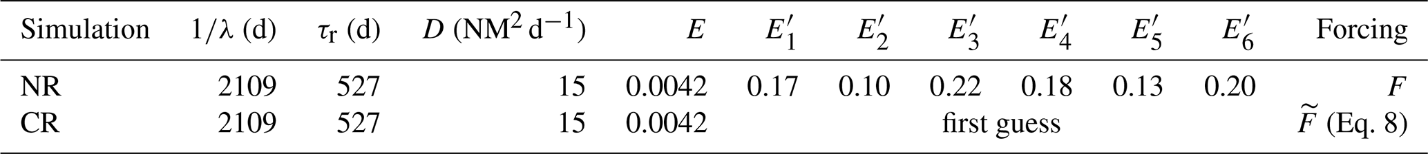
The control run (CR) used to perform the parameter estimate is generated using perturbed forcing fields (Fig. 1). A perturbation is added to the reference forcing fields in order to consider more realistically the discrepancy between the real state of the ocean (represented here by the NR) and the simplified representation of this state by numerical models. The reference forcing fields are perturbed with a white noise whose maximal amplitude is a fraction of the averaged fields. Let F be the considered forcing field and let be its global average (in space and time); we define the perturbed field as
where is the amplitude of the perturbation and is a uniformly distributed random number. The amplitude α is set to 0.1 for all experiments except in Sect. 3.4, where α varies. For small values of F, this perturbation can induce a sign reversal of the forcing. This does not matter for the temperature (degree Celsius; see also Eqs. A5 and A6) or the current velocities (meter per second); primary production (millimoles of carbon per squared meter per day) has however been constrained to positive values. White noise has been preferred to more realistic perturbation to avoid any geographical bias pattern. The implications of this choice are further discussed in Sect. 4.3. Its amplitude, fixed to 10 % of error, is however representative of the mean error estimated for ocean circulation models (Lellouche et al., 2013; Garric and Parent, 2017). The parameters are randomly sampled between 0 and 1. This first guess is used as initialization of the optimization scheme. We run each experiment several times with a different randomly sampled first guess in order to ensure that the inverse model is not sensitive to the initial parameters. The setup of the NR and CR simulations is summarized in Table 1.
A MLE is used as an assimilation module, used here to estimate model parameters from observations. Its implementation is based on an adjoint technique (Errico, 1997) to iteratively optimize a cost function that represents the discrepancy between model outputs and observations. This approach conforms to current practices. More details about the implementation of this approach in SEAPODYM can be found in Senina et al. (2008) and Lehodey et al. (2015).
2.3.2 Synthetic observations
In the framework of OSSE, we perform estimation experiments with different sets of synthetic observation points of size Ne=400. The synthetic observations are sampled from the different configurations introduced in the previous section. Let M be the number of points in a given configuration. If M<Ne, we consider that the configuration is too singular to be relevant for our study and it is ignored. If M>Ne, we randomly extract a subsample of observation points. In order to study the influence of one indicator at a time, we compare experiments for which the regime of the studied indicator varies and the regime of the other indicator variables remains fixed. In the following we call primary variable the studied indicator variable and secondary variables the ones whose regimes are fixed. For a given group of experiments, we check that the configurations are comparable to each other by ensuring that the distribution of all secondary variables is similar (see marginal distribution plots in Sect. 3.2.1). If this not the case, they are not reported. A random sampling of observations within each configuration is preferred to a more realistic observation network to avoid any geographical bias. But this choice is discussed in Sect. 3.4, where realistic networks are tested. The coverage in terms of observation numbers is however quite realistic. We use 400 observations in our experiments, which at the resolution of the model ( month) correspond, for example, to the deployment of six moorings during 5 years.
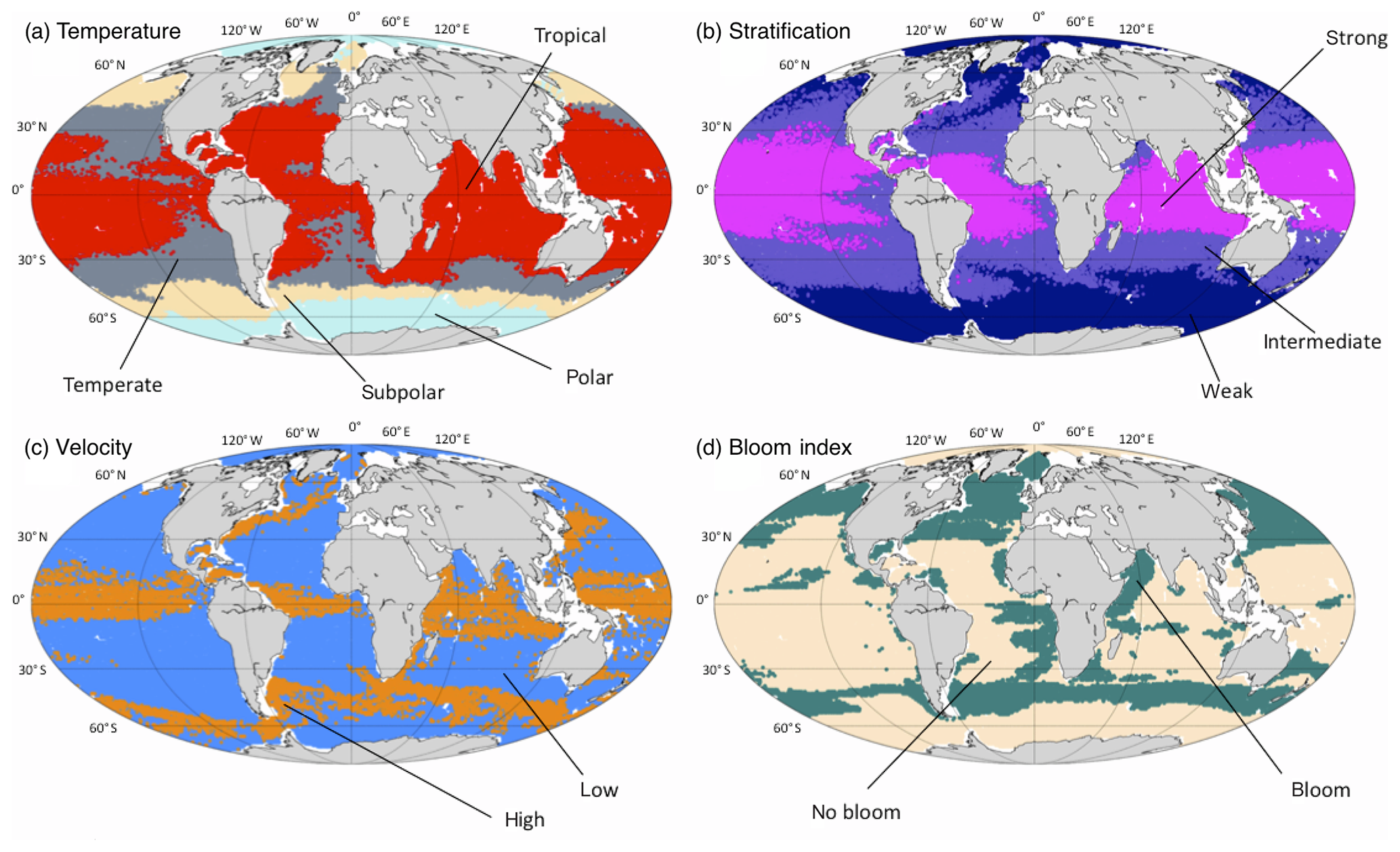
Figure 2Spatial division of the different regimes as defined in Table 2. (a) Temperature: polar (pale blue), subpolar (yellow), temperate (gray) and tropical (red). (b) Stratification: weak (dark blue), intermediate (purple) and strong (magenta). (c) Current velocities: low (blue) and high (orange). (d) Bloom index: bloom (green) and no bloom (beige). Each point of the subset SN has been plotted at its spatial location with a color corresponding to the regime it belongs to.
2.4 OSSE system evaluation metrics
The estimation experiments are evaluated using three metrics: (i) the performance of the estimation, (ii) its accuracy and (iii) its convergence speed.
- (i)
The performance is measured with the mean relative error between the estimated coefficients and the reference coefficients as defined in Lehodey et al. (2015) (Eq. 9).
- (ii)
The accuracy is measured by the residual value of the likelihood which provides a good estimate of the discrepancy between the estimated and the observed biomass.
- (iii)
The convergence speed is measured by the iteration number of the optimization scheme.
The residual likelihood and iteration number metrics are provided by the Automatic Differentiation Model Builder (ADMB) algorithm (Fournier et al., 2012) that is used to implement the MLE. Each metric provides different and independent information. For example, it is possible to obtain good performance and bad accuracy with an experiment that estimates correctly the energy transfer parameters for the different functional groups but over- or underestimates the total amount of biomass. The performance is generally used to discriminate between the different experiments since the aim of the study is to find the networks that better estimate energy transfer coefficients and thus directly minimize the error Er (Eq. 9). However, the accuracy and precision of the experiment are also discussed below. The convergence is necessary to ensure that the optimization problem is well defined.
3.1 Environmental regimes clustering
The number of points per regime, obtained from the clustering (Sect. 2.2) and defined for each environmental variable (Table 2), shows a large variability. Some regimes represent a larger amount of observable points. For instance, the tropical-temperature regime covers 31 % of the observable points. Almost 50 % of the observable points show a weak stratification and only 10 % of them have a positive bloom index or high velocities. When they are shown on a map (Fig. 2) these regimes reproduce classical spatial patterns described in the scientific literature (Fieux and Webster, 2017). The regimes of the temperature variable (𝒯) show a latitudinal distribution. The polar regime (𝒯1) is located south of the polar front (Southern Hemisphere) and in the Arctic Ocean. The subpolar regime is located between the polar front and the south tropical front (Southern Ocean), in the subpolar gyre region (North Atlantic), and in the Bering Sea (North Pacific). The temperate regime covers the subtropical zones of the Southern Atlantic, Indian and Pacific oceans, located north of the south tropical front, and extends as well in the eastern part of the Atlantic and Pacific Ocean. The tropical regime covers most of the tropical ocean and the Indian Ocean. The regimes of the stratification variable (𝒮) are also structured according to the latitude, as stratification depends on the temperature. The stratification decreases from the tropical oceans (where the surface waters are warm compared to the deep waters) to the pole (where the surface waters are almost as cold as the deep waters). The regimes of the surface velocity norm (𝒱) highlight the main energetic structures of the oceanic circulation. The high-surface-current regime thus covers the intense jet-structured equatorial currents, the western boundary currents (the Gulf Stream in the Atlantic and the Kuroshio in the Pacific), the Agulhas Current along the South African coast and the Antarctic Circumpolar Current in the Southern Ocean. The regimes of the bloom index (ℬ) separate mostly the productive regions (North Atlantic and North Pacific, Southern Ocean, eastern side of the tropical Atlantic, along the African coast) from the nonproductive regions (center of subtropical gyres mostly, as well as coastal regions of the Arctic and Antarctic).
Table 2Outcome of the clustering method (Sect. 2.2). For each indicator variable (temperature 𝒯, stratification 𝒮, velocity 𝒱 and bloom index ℬ), the number n of clusters, and the center and size (no. observable) of each cluster (regimes) are given, as well as the proportion of all observable points it represents.
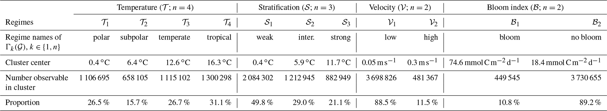
Based on these results, we construct all possible configurations, using the methodology described in Sect. 2.2. Then the configurations are selected to perform the OSSEs presented in Sect. 2.3. The choice of the configuration is limited by the number of observation points available in each of them. Among the 48 possible configurations, 21 of them are nearly empty as they contain less than 0.5 % of all observable points. They are thus considered nonexistent. In addition, we study the influence of the primary variable by selecting only groups of configurations whose distributions along secondary variables are similar. This leads to a selection of seven groups of experiments (Table 3). The purpose of the first three groups of Experiment 1a–b, c–d and e–f is to study the influence of the velocity regimes 𝒱1 and 𝒱2. The group of Experiment 2a–d is used to study the influence of the temperature regimes 𝒯1, 𝒯2, 𝒯3 and 𝒯4. The group Experiment 3a–c is used to investigate the influence of the stratification index regimes 𝒮1, 𝒮2 and 𝒮3. Finally, Experiment 4a–b and c–d evaluate the impact of the bloom index regimes ℬ1 and ℬ2.
3.2 Estimation performance with respect to environmental conditions
Table 3 shows the selected configurations for each experiment (usually abbreviated as Exp. in the following) as well as their evaluation metrics. All experiments converged after 16 to 28 iterations. This confirms that the optimization problem is well defined. Since the number of iterations is partially dependent on the random initial first guess, it is not used as a criterion of discrimination between experiments.

Figure 3Mean relative error (Er in %, Eq. 9) on each coefficients for (a) Exp. 1c and d, which present the following tested regimes: high versus low velocities in temperate temperatures, weak-stratification regimes and bloom regimes; (b) Exp. 2a, 2b, 2c and 2d, which compares polar, subpolar, temperate and tropical temperatures in weak-stratification, low-velocity and bloom regimes; (c) Exp. 3a, b and c, which compares weak, intermediate and high stratification in tropical-temperature, low-velocity and no-bloom regimes; and (d) Exp. 4c and d: bloom versus no-bloom regimes in tropical temperatures, strong stratification and low velocities.
3.2.1 Influence of the horizontal current velocity
The influence of the current velocity regimes (high-current-velocity system or low-current-velocity system) on the performance of the parameter estimation is studied considering three groups of experiments (Table 3, Exp. 1a to f). The observation points are randomly sampled in a subset of the considered configuration for which the primary variable is the current velocity norm 𝒱.
From these sets of experiments, it appears that the performance of the parameter estimation decreases with higher current velocity at the observation points. This conclusion is valid regardless of the regime of the secondary variables: either low or high temperatures, positive or null bloom index, and weak or strong stratification (Table 3). Lower velocity reduces the error on the estimated energy transfer coefficients for functional groups that are impacted by currents in the epipelagic and upper mesopelagic layers. The currents decrease with depth and are almost uniform over the different regions in the lower mesopelagic layer (not shown). Consequently, the estimate of the parameters for the nonmigrant lower mesopelagic (lmeso) group is not sensitive to the regime of currents (Fig. 3a). Conversely, the estimation is the most sensitive for the epipelagic group, whose dynamics are entirely driven by the surface currents.
Note that the influence of low and high velocities is not explored for all secondary-variable fixed regimes. Indeed, even within fixed regimes, the secondary-variable distribution along observation points might not be statistically comparable between two experiments. This could lead to a potential bias introduced by a secondary variable, which is not the target of the study. For instance, the influence of velocity in a polar temperature regime can be investigated by comparing the configurations (low velocity) and (high velocity). The corresponding estimation experiments (Exp. 1′ and Exp. 1′′) give relative errors of 48 % and 10 % respectively. This result seems contradictory to the conclusions drawn from Exp. 1a–f. But looking at the distributions of the observations along the secondary variables, we can notice that the temperatures are different between the two configurations. While both configurations are considered to be in the polar regime, the temperature in configuration C′ (−0.7 ∘C) is on average lower than the temperature of configuration C′′ (2.1 ∘C) (Fig. 4). Thus Exp. 1′ and Exp. 1′′ measure the combined effect of both velocity and temperature. The lower velocities are coupled with lower temperatures and the higher velocities with higher temperatures. There is a cross-correlation between the velocity (primary variable) and the temperature (secondary variable). Therefore, it is not possible to assess the influence of the velocity on the parameter estimation from these experiments.
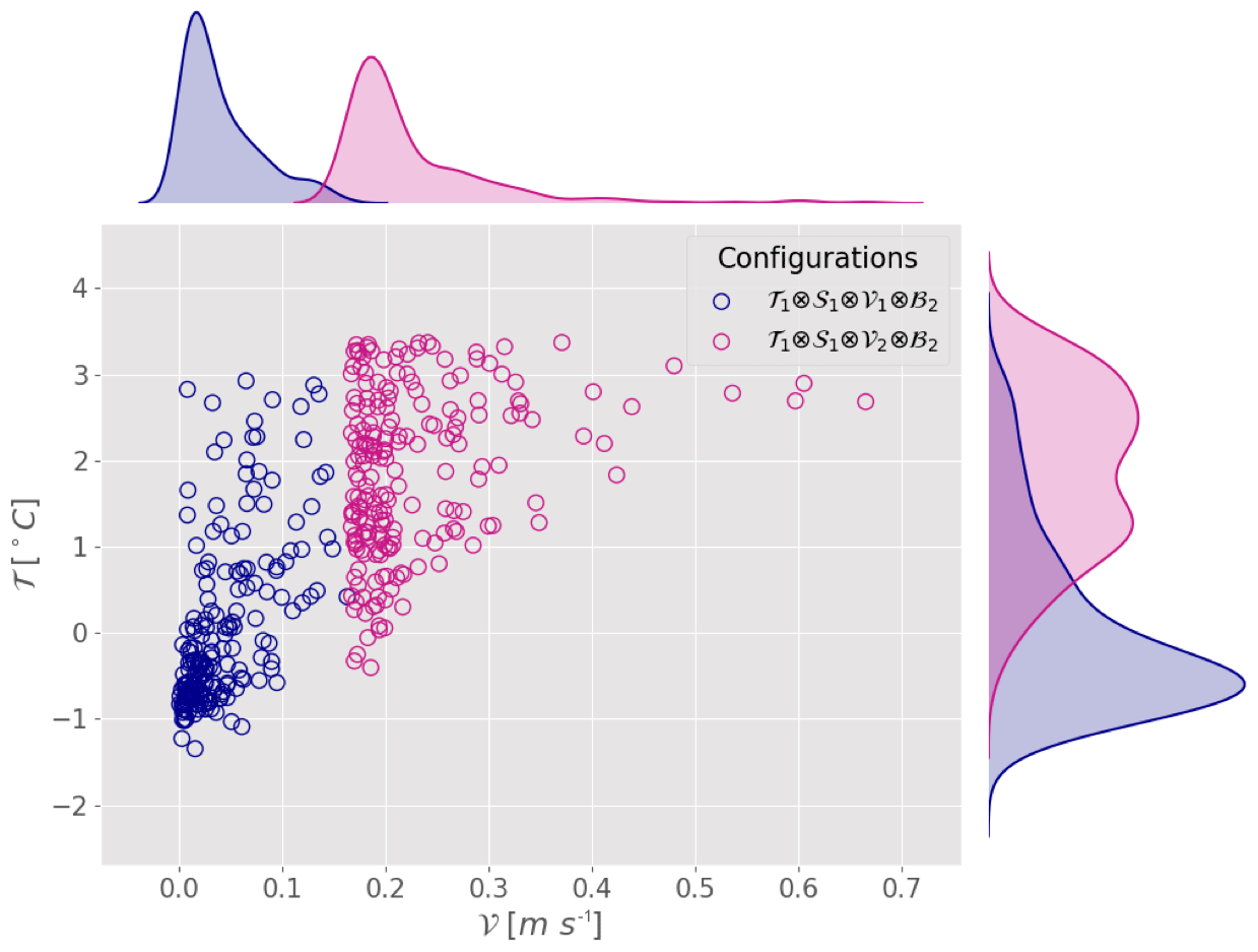
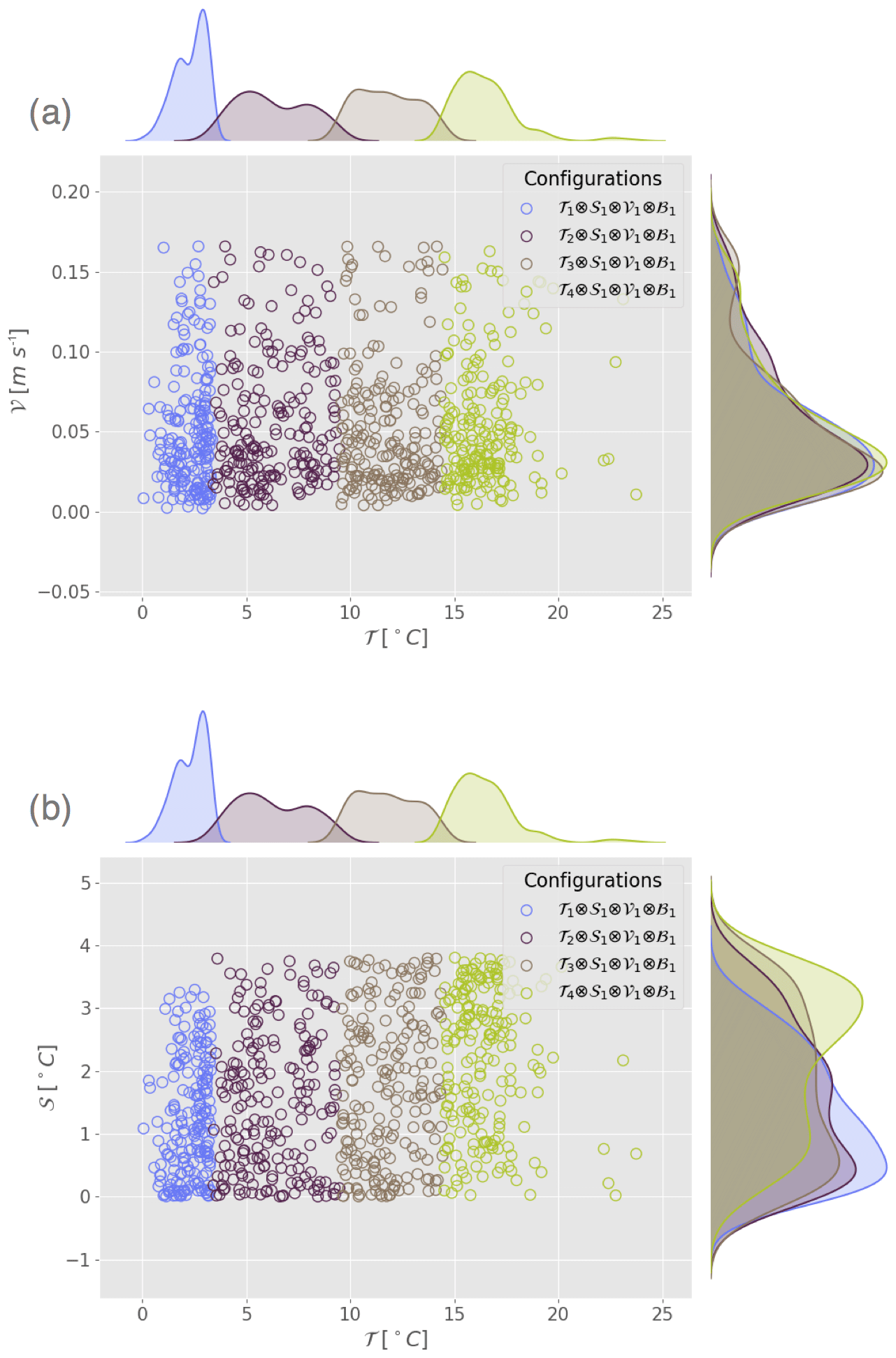
Figure 5Scatter plot and marginal distribution from kernel density estimation in the plane (a) (𝒯,𝒱) and (b) (𝒯,𝒮) for the configurations corresponding to Exp. 3a, b, c and d from Table 3.
Although the distributions of the secondary variables are not always shown in the following experiments, they have been examined to ensure that the OSSE results are not biased by systematic differences in the secondary variables. Experiments with significant cross-correlation between indicator variables are not presented; this concerns 9 out of the 26 possible experiments.
3.2.2 Influence of temperature
In Exp. 2a to d (Table 3), temperature is the primary variable, ranging from polar regime (Exp. 2a) to subpolar (Exp. 2b), temperate (Exp. 2c) and tropical (Exp. 2d) regimes. All other indicator variables (stratification, velocity and bloom index) are secondary variables that are set to weak, low and 1 respectively. Figure 5 shows that the distributions along the secondary variables of each configuration are close enough for the experiments to be compared, avoiding any risk of cross-correlation. The performance of the estimation increases with the temperature (Fig. 3b). The mean error on the parameter estimates decreases respectively from polar (Exp. 2a; 9.1 %) to subpolar (Exp. 2b; 7 %), temperate (Exp. 2c; 3 %) and tropical (Exp. 2d; 1.4 %) configurations (Table 3).
3.2.3 Influence of stratification
The influence of stratification is first investigated with a set of three configurations combining the tropical-temperature regime; low-velocity regime; null bloom index regime; and three regimes of weak (Exp. 3a), intermediate (Exp. 3b) and strong (Exp. 3c) stratification. A marginal distribution plot of observation sets for all experiments (not shown) indicates that the three datasets differ only along the stratification variable (primary variable). The observation points display a temperature between 14 and 17 ∘C, a velocity between 0 and 0.07 m s−1 and a null bloom index for each experiment. The performance decreases with the intensity of stratification (Fig. 3c and Table 3). The mean error is 3.5 % for a weak stratification and a vertical gradient of about 0.4 ∘C (Exp. 3a), 5.9 % for an intermediate stratification with a gradient of about 5.9 ∘C (Exp. 3b) and 8 % for a strong stratification around 11.7 ∘C (Exp. 3c). A strong stratification seems to deteriorate the estimate for all migrant groups (Fig. 3c). These results are not specific to the choice of regimes for the secondary variables. Similar experiments were carried out in a temperate regime (not shown), and, even though the mean error on the estimated parameters is higher on average, the result does not change: weak stratification again leads to a better estimation than strong stratification. The comparison was not fully possible in other temperature or velocity regimes because these configurations are not sufficiently represented.
Table 3Experiment table. List of conducted experiments, their corresponding configurations and the evaluation diagnostics: mean relative error on the coefficients, residual likelihood and number of iterations. The tested regime (primary variable) is specified in the first column, the number of observable belonging to each configuration is indicated in the fourth column, with their relative proportion in brackets. Note that, even if the number of observable points differs for each configuration, the experiments were conducted with 400 observations randomly chosen among the ones belonging to the configuration. The section that describes each experiment is mentioned in the last column.

3.2.4 Influence of primary production
In order to investigate the influence of primary production on the performance of the estimation, we compare the results of estimation in configurations with different bloom index regimes (primary variable). Temperature, stratification index and velocity have been fixed (secondary variables) to subpolar, weak, and low regimes respectively (Exp. 4a and b) and to tropical, strong, and low regimes for Exp. 4c and d. Distributions of the observation points along the secondary variables indicate that the experiments are not biased by secondary variables, as the distributions present similar modes centered at 5 ∘C for the temperature; at 0.5 ∘C for the stratification index; at 0.04 m s−1 for the velocity (Exp. 4a and b); and at 15.5, 11 ∘C and 0.05 m s−1 respectively for Exp. 4c and d (not shown).
Both Exp. 4a and b result in an averaged error of 7 % on the estimated parameters (Table 3). Experiment 4d (averaged error of 8 %) gives a similar value to Exp. 4b. Indeed, Exp. 4d (𝒯4 regime) has a higher temperature than Exp. 4b (𝒯2 regime), but it also has a higher stratification index (the 𝒮3 regime for Exp. 4d and the 𝒮1 regime for Exp. 4b). Following the conclusions from the two previous sections, better performance is achieved when temperature increases, though increasing stratification has the opposite effect. So, the two effects might compensate in this case and result in a similar estimation. However, when considering bloom regions (Exp. 4c), the estimation error falls to 1.5 % on average. In addition, this experiment estimates the energy transfer coefficients for migrant micronekton groups with less than 1 % error (Fig. 3d). According to our results, the primary production and the regimes of the bloom index do not always play a role in the performance of the parameter estimation. A positive bloom index appears to improve the performance of the estimation at high temperatures only.
3.3 Global map of parameter estimation errors
When considering all possible experiments, and given the fact that all these configurations are associated with specific locations and times, it is possible to represent a global map of averaged estimation errors (Eq. 9). This map (Fig. 6) shows that, on average, the error increases from the Equator towards the poles. The lowest performances (errors >40 %) are mostly found in the Arctic and Southern Ocean. Low performances are also found at some specific locations (e.g., along the main currents). The signature of the Antarctic Circumpolar Current is found in the Southern Ocean with an error over 10 %. Similarly, the signature of the North Atlantic Drift can be seen with a patch of high errors between Canada and Ireland (Figs. 2c and 6). The patch of high errors in the North Pacific Ocean, however, is difficult to interpret. The equatorial regions show interesting patterns that are similar across the three oceans. In the vicinity of the Equator, good performances are observed (mean error ∼2 %). On both the northern and southern sides of this low error band, the performance is decreased, with errors reaching about 8 %. The equatorial regions are characterized by strong currents and warm surface waters. As described above, these environmental features have opposite effects on the performance of the estimation. Therefore, a possible explanation of this distribution of errors is that water temperature is high enough to overcome the effect of currents in the equatorial band, but when moving poleward the temperature decreases cannot compensate anymore for the negative effect of currents, which is still quite strong. It should be noted that the map presented in Fig. 6 was obtained for a given set of forcing fields (temperature, velocity, primary production). It is thus dependent on the simulation that is used. The regime dependence of the estimation performance is however independent of the simulation.

3.4 Testing realistic networks
The above experiments are based on random selection of observation points within a large subset. This technique was chosen to avoid any bias related to the temporal or spatial potential autocorrelation of observation networks. However, sampling at sea is rarely randomly distributed and can generate correlations. To relax this strong assumption, we perform experiments based on positions from real acoustic transects (underway ship measurements). Two regions are compared using the transects from the PIRATA cruises in the equatorial Atlantic (Bourlès et al., 2019) and those from the British Antarctic Survey (BAS) close to the Antarctic Peninsula (Fig. 7).
The same forcing, method and initial parameterization were used with a random noise amplitude (α) increasing from 0 to 0.2. Subsets of Ne=400 observations were selected along the transects to run the experiments. The resulting averaged relative error on the coefficients is shown as a function of the amplitude of perturbation (Fig. 8a) for both networks. It appears that the estimation error increases with the amplitude of the error introduced on the forcing field. Also, regardless of the intensity of the perturbation, the estimation error is always lower when using PIRATA observation networks than BAS observation networks. These results are fully consistent with the previous results indicating that networks located in tropical warm waters, as for PIRATA, give better estimates than the ones located in cold waters, as for the BAS (Fig. 8b). This should give confidence in the fact that our results are robust when the random sampling hypothesis used in the previous section is relaxed and that more realistic sampling designs are considered. Here in particular, the temporal autocorrelation of the different samplings is very strong since PIRATA and BAS are both underway ship measurements taken from 2-month cruises, repeated annually. The results seem much less dependent on the exact design of the samplings and the seasonality of the measurements than on their actual geographical location. Oceanic conditions of the observations (correlated to their geographical location) are the first order of sensitivity. In this sense, the PIRATA network is thus a very promising observatory for the micronekton, especially since it already includes a complete set of various physical and biogeochemical parameter measurements (Foltz et al., 2019).
In the following, we will discuss a possible theoretical interpretation of the outcome of the estimation experiments (Sect. 4.1) and a potential application of our results (Sect. 4.2). Section 4.3 closes this discussion examining the particular framework used to conduct this study and opening some perspectives for future work.
4.1 An interpretation of the performance in terms of observability
The differences in the performance of parameter estimation can be interpreted in the light of the characteristic timescales of physical and biological processes. The parameters we want to estimate () control the energy transfer efficiency between the primary production (PP) and micronekton production (P) (Eq. A3; Appendix A). These parameters are thus directly related to the relative amount (Pi) of P in each functional group i at age τ=0, and we have
where EPP is the total energy transfer from the primary production to the midtrophic level (all functional groups together) and c a conversion coefficient (see Appendix A). It is possible to rewrite the initial condition (Eq. A3) as a system of six equations involving the energy transfer coefficients.
where , with ρ defined as , is the ratio of age 0 potential micronekton production in the layer , at the time of the day (for day and night).
The predicted micronekton biomass at a given time and location (grid cell) results from two main mechanisms. First, the potential production (P) evolves in time from age τ=0 and is redistributed by advection and diffusion until the recruitment time τr when it is transferred into biomass (B). Second, the biomass is built by the accumulation of recruitment over time in each grid cell and is lost due to a temperature-dependent mortality rate, while the currents redistribute the biomass spatially. The observations correspond to the relative amount of biomass in each layer, i.e., the ratios of biomass (Eq. A7), where to is the time at which the observation is collected. Therefore, the observation will contain more information about the energy transfer parameters we want to estimate if is close to (Eq. 11). This requires that the integrated mixing and redistribution of biomass during the elapsed time between age 0 of potential production and the time of observation (i.e., at least the recruitment time) are as weak as possible. This can be achieved in two ways: either (i) the currents are weak so that the advection of biomass is also weak (but the diffusion will still remain) or (ii) the temperature is high, leading to a short recruitment time with a reduced period of transport, mixing and redistribution of biomass (Eq. A5). These two mechanisms can explain why warm temperatures and weak currents were found to improve the estimations compared to cold temperatures and high velocities (Sect. 3.2.1 and 3.2.2). An additional effect of warm temperature is that it induces a higher mortality rate (Eq. A6). When warm waters are combined with high primary production (e.g., the equatorial upwelling region), there is a rapid turnover of biomass, and the relative ratios of biomass by layer are closer to the initial ratio of production and thus to the energy transfer efficiency coefficients. Conversely, at cold temperature, the mortality rate is lower; biomass is accumulated from recruitment events and carries with it the integrated mixing and the perturbed ratio structures. This can explain why, at warm temperature, high productivity is needed for a better estimation (Sect. 3.2.4). A side effect is that if temperature is not homogeneous across layers, then the mortality rate λ will differ for each functional group, depending on the layers it inhabits. This will be an additional driver of perturbation on the observed ratios of biomass compared to the initial ratios of potential production. This is consistent with the result that a strong thermal stratification degrades the performance of estimation (Sect. 3.2.3).
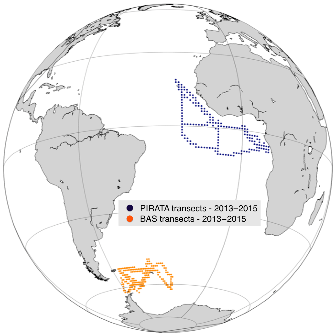
Figure 7Map of PIRATA and BAS ship transects for the years 2013–2015.
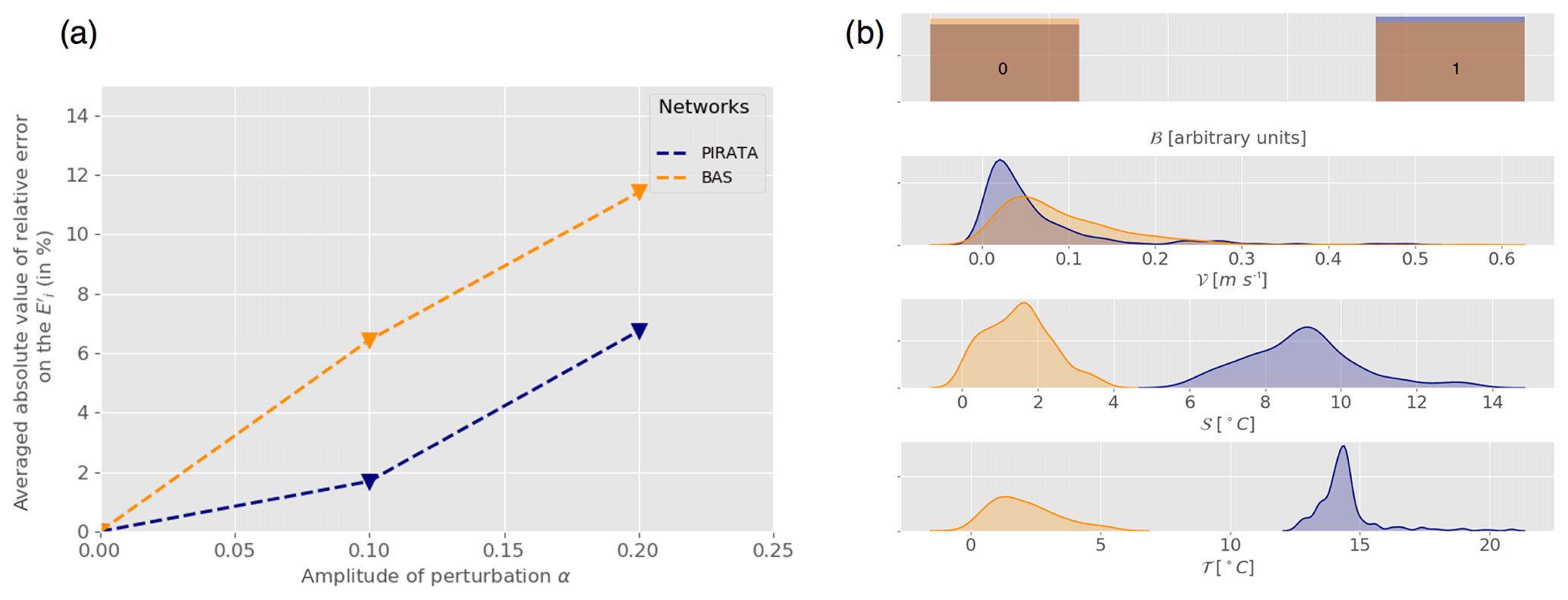
Figure 8(a) Mean relative error on the coefficients Er (in %, Eq. 9) as a function of the perturbation amplitude α (Eq. 8) for PIRATA (blue) and BAS (orange) observation networks. (b) Statistical distribution of all PIRATA (blue) and BAS (orange) observation location indicator variables: bloom index (ℬ), velocity norm (𝒱), stratification index (𝒮) and temperature (𝒯) estimated using kernel density estimation (Silverman, 2018).
An observation will thus be the most effective for the estimation of parameters if it carries the information of the initial distribution of primary production into functional groups. This is the case if the biomass is renewed quickly enough compared to the time it takes for the currents and diffusive coefficient to mix it. This condition can be seen in terms of equilibrium between the biological processes (production, recruitment and mortality) and the physical processes (advection and diffusion). For an observation to be the most useful to the parameter estimation, it is necessary that the characteristic timescale governing biological processes (τβ) is shorter than the one governing physical processes (τϕ) at the location of the observation: τβ≪τϕ.
This interpretation highlights the problem of observability of the parameters from the measurements ρK,Ω(B). The parameters are directly observable at the age τ=0 of the production, but the measurements and the information we can get on the system are available only after a time τr. The observability will then be the better if the observable variables have not changed too much during the time τr (short τr, slow ocean dynamics). This is intrinsically linked to governing equations of the system (Eqs. A1–A3) and therefore should not be dependent on the framework of the study.
4.2 Towards ecoregionalization?
The clustering approach we propose allowed the identification of oceanic regions that provide optimal oceanic characteristics for our parameter estimation. It separates regions where the distribution of biomass is driven by physical processes from regions where it is driven by biological processes. This could be seen as a new definition of ecoregions based on similar ecosystem structuring dynamics. The definition of ocean ecoregions has been proposed based on various criteria (Emery, 1986; Longhurst, 1995; Spalding et al., 2012; Fay and McKinley, 2014; Sutton et al., 2017; Proud et al., 2017). A convergence of these different approaches to identify regions characterized by homogeneous mesopelagic species communities would be of great interest to facilitate the modeling and biomass estimate of the mesopelagic components. Acoustic observation models could be developed and validated at the scale of these regions. Then, the observation models integrated into ecosystem and micronekton models as the one used here would serve to convert their predicted biomass into an acoustic signal to be directly compared to all acoustic observations collected in the selected region. This approach would allow us to account for (and estimate) the sources of biases and errors linked to acoustic observations directly in the data assimilation scheme.
4.3 Limitations and perspectives
We have chosen to model the error between the true state of the ocean and the modeled state by adding a white noise perturbation to the forcings of the NR as input of the CR. Our idealized approach does not take into account the possible spatial distribution of uncertainty and errors of ocean models, and other approaches would be interesting to explore. For instance, implementing an error proportional to the deviation of the climatological field should be more realistic because it would be based on the natural and intrinsic variability of the ocean. Indeed, we expect forcing fields to be less accurate where the ocean has strong variability. However, for the purpose of our study, a spatial homogeneous error was preferable to avoid introducing any bias. Random noise ensures that the results obtained in different locations are directly comparable. Conducing a sensitivity analysis with respect to the choice of forcing error modeling was beyond the scope of this study. In addition to the uncertainty of ocean model outputs, other sources of uncertainties remain to be explored to progress toward more realistic estimation experiments. For instance, we considered that the observation operator (Eq. A7) is perfect but field observations are always tainted by errors. The micronekton biomass estimates at sea require a chain of extrapolation and corrections to account for the sampling gear selectivity and the portion of water layer sampled. For acoustic data, many factors need to be considered sources of potential error: the correction with depth, the target strength of species, and the intercalibration between instruments and the signal processing methods (Handegard et al., 2009, 2012; Kaartvedt et al., 2012; Proud et al., 2018). This is an important research domain that requires the combination of multiple observation systems, including new emerging technologies such as broadband acoustics, optical imagery and environmental DNA to reduce overall bias in estimates of micronekton biomass (e.g., Kloser et al., 2016) and use those estimates to assess, initiate and assimilate into ecosystem models. Finally, the results of the clustering approach need to be confirmed with other ocean circulation model outputs, especially at higher resolution to check the impact of the mesoscale activity on the definition of optimal regions for energy transfer efficiency estimation. In a future study, in addition to testing the impact of introducing noises in the observations, the same approach could be used to also directly estimate the model parameters that control the relationship between the water temperature and the time of development of micronekton organisms. Other perspectives may include a study of the sensitivity to the design of the samplings (the impact of moored instruments in comparison with underway measurements), in the continuity of the work of Lehodey et al. (2015).
Understanding and modeling marine ecosystem dynamics is considerably challenging. It generally requires sophisticated models relying on a certain number of parameterized physical and biological processes. SEAPODYM-MTL provides a parsimonious approach with only a few parameters and a MLE to estimates these parameters from observations. Among them, the energy transfer efficiency coefficients are of great importance because they directly control the biomass of micronekton functional groups, including those that undergo DVM and contribute to the sequestration of carbon dioxide into the deep ocean (Davison et al., 2013; Giering et al., 2014; Ariza et al., 2015). Therefore, a correct assessment of energy transfer coefficients is crucial for climate studies. Given the high cost of observations at sea, the design of optimal observational networks through simulation experiments (OSSEs) is a valuable approach before the deployment of such platforms. Our objective was different from most OSSE studies designed to estimate the impact of an observing system from the difference in the errors made by each experiment (Fujii et al., 2019). Here the objective was to determine the optimal observations to estimate the set of invariant fundamental parameters of the model. This study provides insights for implementing such observations, based on the definition of oceanic regions using only four variables: the depth-averaged temperature, a thermal stratification index, the surface current velocity norm and a bloom index. Experiments that were conducted in these regions with random sampling or based on realistic existing networks have shown that the quality of the MLE for the energy transfer efficiency coefficients is mainly linked to environmental conditions. We found that observations from warm temperature regions (such as temperate or tropical regions) were more effective than those from cold regions. The presence of a bloom at the location of observation also improves the performance of the estimation (especially in warm environment). Conversely, high-temperature stratification and high intensity of currents are both found to deteriorate the estimate. Thus, an optimal combination of environmental factors is found at a global scale for productive, warm and moderately stratified waters, with weak dynamics, such as the eastern side of the tropical oceans. In terms of estimation performance, some functional groups are more affected by the regime variable than other. This is the case for the migrant groups that are very sensitive to the stratification or the bloom index regime for instance. However, no systematic differences between the different groups are noted. The main limitation in this study is certainly the absence of realistic modeling of the different sources of errors: the error between the modeled and the true state of the ocean has been modeled with a white noise perturbation that does not allow for spatially inhomogeneous errors. And the observations have been assumed to be directly proportional to biomass. The absence of a realistic observation model converting the acoustic signal into biomass (Jech et al., 2015) prevents accounting for the different types of observation errors. Future studies should include these missing components. An interpretation of the results in terms of balance between characteristic times of biological and physical processes has been proposed, pointing out a mathematical problem of observability. Hopefully this study will help in the next development of observing networks for micronekton and more generally will provide a useful methodology for future research aiming at investigating the influence of environmental conditions on the observability of some parameters. In any case, we believe it is a next step in the modeling of midtrophic ecosystems, with implications ranging from fisheries management to climate studies.
SEAPODYM-MTL is based on a system of advection–diffusion–reaction equations for each functional group i, i∈{1…6}, involving two state variables: the potential production Pi (expressed in grams of wet weight per squared meter per day, ) and the biomass Bi (expressed in grams of wet weight per squared meter, g WW m−2):
where x and y, t, and τ are the variables for space, time, and age respectively. u,v (m s−1) and T (∘C) are the current velocities and temperature respectively. These variables are integrated over each layer K, K∈{1…3} and weighted by the time each functional group i spends in the layer. D is the diffusion coefficient accounting for both the physical diffusion and the ability of micronekton organisms to swim short distances. τr (days) is the recruitment coefficient corresponding to the age for which the potential production converts into biomass of micronekton. λ (d−1) is the mortality coefficient which accounts for natural mortality. Note that these two last parameters depend on the temperature.
The initial conditions for this system are
where B0 and P0 are obtained by spinup, PP (in millimoles of carbon per cubic meter per day, ) is the net primary production, EPP (adimensional) is the total energy transfer from the primary production to the midtrophic level, (adimensional) is the distribution of this energy into the different functional groups, c is the conversion coefficient between mmol C and g WW and , and zeu is the euphotic depth (in meters).
Following Lehodey et al. (2010), the recruitment and mortality coefficients are parameterized as
with τr0=527 d and d−1.
with and λc=0.125 d−1
Note that these coefficient are also defined for negative temperature values.
A module estimates SEAPODYM-MTL parameters using a variational data assimilation method: a maximum likelihood estimation (MLE) (Senina et al., 2008). This method minimizes a cost function (the likelihood) that measures the distance between the biomass predicted by the model and the observed biomass. As the model outputs and the observations are not directly comparable, they are transformed with an observation model operator ℋ. ℋ is defined for each layer K as
where K(i,ω) denotes the layer that the functional group number i occupies at the time of the day ω. ℋ gives for each layer the relative amount of biomass that we call ratio (Lehodey et al., 2015).
The gradient of the likelihood function is computed using the adjoint state method. The parameters are then estimated using a quasi-Newton algorithm implemented by the Automatic Differentiation Model Builder (ADMB) algorithm (Fournier et al., 2012). SEAPODYM-MTL and the exact formulation of the cost function are described in detail in Lehodey et al. (2015).
Physical oceanographic data of the free GLORYS2V4 ocean circulation simulation are available at the Copernicus Marine Environment Monitoring Service (CMEMS: http://marine.copernicus.eu/services-portfolio/access-to-products/?option=com_csw&view=details&product_id=GLOBAL_REANALYSIS_PHY_001_025; last accessed: 7 January 2020). Satellite derived primary production data (VGPM model) are made available by the Ocean productivity team at Oregon State University (http://orca.science.oregonstate.edu/1080.by.2160.monthly.hdf.vgpm.m.chl.m.sst.php, Behrenfeld and Falkowski, 1997, last accessed: 7 January 2020). The SEAPODYM-MTL simulation is provided as a product of the CMEMS catalogue (http://marine.copernicus.eu/services-portfolio/access-to-products/?option=com_csw&view=details&product_id=GLOBAL_REANALYSIS_BIO_001_033; last accessed: 7 January 2020).
All authors contributed to the design of the study. AD developed the method, conducted the experiments, analyzed the results and wrote the original manuscript. AC and OT contributed to the development of the parameter estimation component of SEAPODYM-MTL. OT prepared the forcing fields and contributed to the revision of the manuscript. PL coordinated the AtlantOS activity at CLS and contributed to the analysis of results and the revision of the manuscript.
The authors declare that they have no conflict of interest.
This study has been conducted using E.U. Copernicus Marine Service Information. The authors thank the Groupe Mission Mercator Coriolis (Mercator Ocean) for providing the ocean general circulation model FREEGLORYS2V4 simulation and Jacques Stum and Benoit Tranchant at Collecte Localisation Satellite for processing satellite primary production and ocean reanalysis data. We also thank Bernard Bourlès and Jérémie Habasque from the Institut de Recherche pour le Développement and Sophie Fielding from the British Antarctic Survey for making the PIRATA (http://www.brest.ird.fr/pirata/pirata, last access: 7 January 2020) and BAS (https://www.bas.ac.uk/project/poets-wcb, last access: 7 January 2020) cruise trajectories available. The authors are also grateful to Susanna Michael and two anonymous reviewers whose comments and suggestions helped improve the paper.
This research has been supported by the Horizon 2020 (grant no. AtlantOS (633211) and MEESO (817669)).
This paper was edited by Stefano Ciavatta and reviewed by Jann Paul Mattern and one anonymous referee.
Ariza, A., Garijo, J., Landeira, J., Bordes, F., and Hernández-León, S.: Migrant biomass and respiratory carbon flux by zooplankton and micronekton in the subtropical northeast Atlantic Ocean (Canary Islands), Prog. Oceanogr., 134, 330–342, 2015. a, b
Arnold, C. P. and Dey, C. H.: Observing-systems simulation experiments: Past, present, and future, B. Am. Meteorol. Soc., 67, 687–695, 1986. a
Barnier, B., Madec, G., Penduff, T., Molines, J.-M., Tréguier, A.-M., Le Sommer, J., Beckmann, A., Biastoch, A., Böning, C. W., Dengg, J., Derval, C., Durand, E., Gulev, S., Rémy, E., Talandier, C., Theetten, S., Maltrud, M. E., McClean, J., and De Cuevas, B.: Impact of partial steps and momentum advection schemes in a global ocean circulation model at eddy-permitting resolution, Ocean Dynam., 56, 543–567, https://doi.org/10.1007/s10236-006-0082-1, 2006. a
Behrenfeld, M. and Falkowski, P.: Photosynthetic rates derived from satellite-based chlorophyll concentration, Limnol. Oceanogr., 42, 1–20, http://orca.science.oregonstate.edu/1080.by.2160.monthly.hdf.vgpm.m.chl.m.sst.php, 1997. a
Benoit-Bird, K., Au, W., and Wisdoma, D.: Nocturnal light and lunar cycle effects on diel migration of micronekton, Limnol. Oceanogr., 54, 1789–1800, 2009. a, b
Bourlès, B., Araujo, M., McPhaden, M. J., Brandt, P., Foltz, G. R., Lumpkin, R., Giordani, H., Hernandez, F., Lefèvre, N., Nobre, P., Campos, E., Saravanan, R., Trotte-Duhà, J., Dengler, M., Hahn, J., Hummels, R., Lübbecke, J. F., Rouault, M., Cotrim, L., Sutton, A., Jochum, M., and Perez, R. C.: PIRATA: A sustained observing system for tropical Atlantic climate research and forecasting, Earth Space Sci., 6, 577–616, 2019. a
Davison, P.: The specific gravity of mesopelagic fish from the northeastern pacific ocean and its implications for acoustic backscatter, J. Mar. Sci., 68, 2064–2074, 2011. a, b
Davison, P., Checkley Jr., D., Koslow, J., and Barlow, J.: Carbon export mediated by mesopelagic fishes in the northeast Pacific Ocean, Prog. Oceanogr., 116, 14–30, 2013. a, b, c
Davison, P. C., Koslow, J. A., and Kloser, R. J.: Acoustic biomass estimation of mesopelagic fish: backscattering from individuals, populations, and communities, ICES J. Mar. Sci., 72, 1413–1424, 2015. a
Emery, W. J.: Global water masses: summary and review, Oceanol. Acta, 9, 383–391, 1986. a
Errico, R. M.: What is an adjoint model?, B. Am. Meteorol. Soc., 78, 2577–2592, 1997. a
Fay, A. R. and McKinley, G. A.: Global open-ocean biomes: mean and temporal variability, Earth Syst. Sci. Data, 6, 273–284, https://doi.org/10.5194/essd-6-273-2014, 2014. a
Garric, G. and Parent, L.: Quality Iinformation Document For Global Ocean Reanalysis Products: GLOBAL-REANALYSIS-PHY-001-025, Issue 3.5, p. 48, 2017. a
Fieux, M. and Webster, F.: The planetary ocean, Current natural sciences, EDP Sciences, 2017. a
Foltz, G. R., Brandt, P. Richter, I., Rodríguez-Fonseca, B., Hernandez, F., Dengler, M., Rodrigues, R. R., Schmidt, J. O. , Yu, L. , Lefevre, N., Cotrim, L., Cunha, D., McPhaden, M. J., Araujo, M., Karstensen, J. , Hahn, J. , Martín-Rey, M., Patricola, C. M., Poli, P., Zuidema, P., Hummels, R., Perez, R. C., Hatje, V., Lübbecke, J. F., Polo, I., Lumpkin, R. , Bourlès, B., Asuquo, F. E., Lehodey, P. , Conchon, A. , Chang, P. , Dandin, P. , Schmid, C. , Sutton, A., Giordani, H. , Xue, Y. , Illig, S. , Losada, T., Grodsky, S. A., Gasparin, F., Lee, T., Mohino, E., Nobre, P., Wanninkhof, R., Keenlyside, N., Garcon, V., Sánchez-Gómez, E., Nnamchi, H. C., Drévillon, M., Storto, A., Remy, E., Lazar, A., Speich, S., Goes, M., Dorrington, T., Johns, W. E., Moum, J. N. , Robinson, C., Perruche, C., de Souza, R. B., Gaye, J. López-Parage, A. T., Monerie, P.- A., Castellanos, P. N., Benson, U., Hounkonnou, M. N., Trotte Duhá, J., Laxenaire, R., and Reul, N.: The tropical atlantic observing system, Front. Mar. Sci., 6, 206, https://doi.org/10.3389/fmars.2019.00206, 2019. a
Fournier, D. A., Skaug, H. J., Ancheta, J., Ianelli, J., Magnusson, A., Maunder, M. N., Nielsen, A., and Sibert, J.: AD Model Builder: using automatic differentiation for statistical inference of highly parameterized complex nonlinear models, Optim. Method. Softw., 27, 233–249, 2012. a, b
Thank you. Fujii, Y., Rémy, E., Zuo, H., Oke, P., Halliwell, G., Gasparin, F., Benkiran, M., Loose, N., Cummings, J., Xie, J., Xue, Masuda, Y. S., Smith, G. C., Balmaseda, M., Germineaud, C., Lea, D. J., Larnicol, G., Bertino, L., Bonaduce, A., Brasseur, P., Donlon, C., Heimbach, P., Kim, Y., Kourafalou, V., Le Traon, P.-Y., Martin, M., Paturi, S., Tranchant, B., and Usui, N.: Observing system evaluation based on ocean data assimilation and prediction systems: on-going challenges and future vision for designing/supporting ocean observational networks, Front. Mar. Sci., 6, 417, https://doi.org/10.3389/fmars.2019.00417, 2019. a
Giering, S., Sanders, R., Lampitt, R., Anderson, T., Tamburini, C., and Boutif, M.: Reconciliation of the carbon budgetin the ocean's twilight zone, Nature, 507, 480–483, 2014. a, b
Gjosaeter, J. and Kawaguchi, K.: A review of the world ressources of mesopelagic fishes, Food Agri. Org., 193–199, 1980. a
Handegard, N., Du Buisson, L., Brehmer, P., Chalmers, S., De Robertis, A., Huse, G., and Kloser, R.: Acoustic estimates of mesopelagic fish: as clear as day and night?, J. Mar. Sci., 66, 1310–1317, 2009. a, b
Handegard, N., Du Buisson, L., Brehmer, P., Chalmers, S., De Robertis, A., Huse, G., and Kloser, R.: Towards an acoustic-based coupled observation and modelling system for monitoring and predicting ecosystem dynamics of the open ocean, Fish Fish., 14, 605–615, 2012. a
Henson, S. A. and Thomas, A. C.: Interannual variability in timing of bloom initiation in the California Current System, J. Geophys. Res.-Ocean., 112, C08007, https://doi.org/10.1029/2006JC003960, 2007. a
Hoffman, R. N. and Atlas, R.: Future observing system simulation experiments, B. Am. Meteorol. Soc., 97, 1601–1616, 2016. a
Irigoien, X.: Large mesopelagic fishes biomass and trophic efficiency in the open ocean, Nat. Commun., 5, 3271, https://doi.org/10.1038/ncomms4271, 2014. a
Jain, A. K., Murty, M. N., and Flynn, P. J.: Data clustering: a review, ACM computing surveys (CSUR), 31, 264–323, 1999. a
Jech, M. J., Horne, J. K., Chu, D., Demer, D. A., Francis, D. T., Gorska, N., Jones, B., Lavery, A. C., Stanton, T. K., Macaulay, G. J., Reeder, D. B., and Sawada, K.: Comparisons among ten models of acoustic backscattering used in aquatic ecosystem research, J. Acoust. Soc. Am., 138, 3742–3764, 2015. a
Kaartvedt, S., Staby, A., and Aksnes, D. L.: Efficient trawl avoidance by mesopelagic fishes causes large underestimation of their biomass, Mar. Ecol. Prog. Ser., 456, 1–6, 2012. a, b
Kanungo, T., Mount, D. M., Netanyahu, N. S., Piatko, C. D., Silverman, R., and Wu, A. Y.: An efficient k-means clustering algorithm: Analysis and implementation, IEEE T. Pattern Anal., 24, 881–892, 2002. a
Kloser, R. J., Ryan, T. E., Keith, G., and Gershwin, L.: Deep-scattering layer, gas-bladder density, and size estimates using a two-frequency acoustic and optical probe, ICES J. Mar. Sci., 73, 2037–2048, 2016. a, b
Kodinariya, T. M. and Makwana, P. R.: Review on determining number of Cluster in K-Means Clustering, Int. J., 1, 90–95, 2013. a
Lehodey, P., Andre, J.-M., Bertignac, M., Hampton, J., Stoens, A., Menkès, C., Mémery, L., and Grima, N.: Predicting skipjack tuna forage distributions in the equatorial Pacific using a coupled dynamical bio-geochemical model, Fish. Oceanogr., 7, 317–325, 1998. a
Lehodey, P., Sennina, I., and Murtugudde, R.: A spatial ecosystem and population dynamics model – modeling of tuna and tuna-like population, Prog. Oceanogr., 78, 304–318, 2008. a, b
Lehodey, P., Murtugudde, R., and Senina, I.: Bridging the gap from ocean models to population dynamics of large marine predators : A model of mid-trophic functional groups, Prog. Oceanogr., 84, 69–84, 2010. a, b, c, d, e, f, g
Lehodey, P., Conchon, A., Senina, I., Domokos, R., Calmettes, B., Jouano, J., Hernandez, O., and Kloser, R.: Optimization of a micronekton model with acoustic data, J. Mar. Sci., 72, 1399–1412, 2015. a, b, c, d, e, f, g
Lellouche, J.-M., Le Galloudec, O., Drévillon, M., Régnier, C., Greiner, E., Garric, G., Ferry, N., Desportes, C., Testut, C.-E., Bricaud, C., Bourdallé-Badie, R., Tranchant, B., Benkiran, M., Drillet, Y., Daudin, A., and De Nicola, C.: Evaluation of global monitoring and forecasting systems at Mercator Océan, Ocean Sci., 9, 57–81, https://doi.org/10.5194/os-9-57-2013, 2013. a
Longhurst, A.: Seasonal cycles of pelagic production and consumption, Prog. Oceanogr., 36, 77–167, 1995. a, b
Proud, R., Cox, M. J., and Brierley, A. S.: Biogeography of the global ocean’s mesopelagic zone, Curr. Biol., 27, 113–119, 2017. a, b
Proud, R., Handegard, N. O., Kloser, R. J., Cox, M. J., and Brierley, A. S.: From siphonophores to deep scattering layers: uncertainty ranges for the estimation of global mesopelagic fish biomass, ICES J. Mar. Sci., 76, 718–733, 2018. a, b
Senina, I., Silbert, J., and Lehodey, P.: Parameter estimation for basin-scale ecosytem-linked population models of large pelagic predators : Application to skipjack tuna, Prog. Oceanogr., 78, 319–335, 2008. a, b, c
Siegel, D., Doney, S., and Yoder, J.: The North Atlantic spring phytoplankton bloom and Sverdrup's critical depth hypothesis, Science, 296, 730–733, 2002. a
Silverman, B. W.: Density estimation for statistics and data analysis, Routledge, 2018. a, b
Spalding, M. D., Agostini, V. N., Rice, J., and Grant, S. M.: Pelagic provinces of the world: a biogeographic classification of the world’s surface pelagic waters, Ocean Coast. Manage., 60, 19–30, 2012. a
St John, M. A., Borja, A., Chust, G., Heath, M., Grigorov, I., Mariani, P., Martin, A. P., and Santos, R. S.: A dark hole in our understanding of marine ecosystems and their services: perspectives from the mesopelagic community, Front. Mar. Sci., 3, 31, https://doi.org/10.3389/fmars.2016.00031, 2016. a, b
Sutton, T. T., Clark, M. R., Dunn, D. C., Halpin, P. N., Rogers, A. D., Guinotte, J., Bograd, S. J., Angel, M. V., Perez, J. A. A., Wishner, K., Haedrichj, R. L., Lindsayk, D. J., Drazenl, J. C., Vereshchakam, A., Piatkowskin, U., Moratoo, T., Błachowiak-Samołykp, K., Robisonq, B. H., Gjerder, K. M., Pierrot-Bultss, A., Bernalt, P., Reygondeauu, G., and Heinov, M.: A global biogeographic classification of the mesopelagic zone, Deep-Sea Res. Pt. I, 126, 85–102, 2017. a, b
Tibshirani, R., Walther, G., and Hastie, T.: Estimating the number of clusters in a data set via the gap statistic, J. R. Stat. Soc. B, 63, 411–423, 2001. a
Volk, T. and Hoffert, M. I.: Ocean carbon pumps: Analysis of relative strengths and efficiencies in ocean-driven atmospheric CO2 changes, The carbon cycle and atmospheric CO2: natural variations Archean to present, 32, 99–110, 1985. a
Zaret, T. and Suffern, J.: Vertical migration in zooplankton as a predator avoidance mechanism, Limnol. Oceanogr., 21, 804–816, 1976. a, b