the Creative Commons Attribution 4.0 License.
the Creative Commons Attribution 4.0 License.
 | 09 Mar 2021
Radium-228-derived ocean mixing and trace element inputs in the South Atlantic
Walter Geibert
E. Malcolm S. Woodward
Neil J. Wyatt
Maeve C. Lohan
Eric P. Achterberg
Gideon M. Henderson
Trace elements (TEs) play important roles as micronutrients in modulating marine productivity in the global ocean. The South Atlantic around 40∘ S is a prominent region of high productivity and a transition zone between the nitrate-depleted subtropical gyre and the iron-limited Southern Ocean. However, the sources and fluxes of trace elements to this region remain unclear. In this study, the distribution of the naturally occurring radioisotope 228Ra in the water column of the South Atlantic (Cape Basin and Argentine Basin) has been investigated along a 40∘ S zonal transect to estimate ocean mixing and trace element supply to the surface ocean. Ra-228 profiles have been used to determine the horizontal and vertical mixing rates in the near-surface open ocean. In the Argentine Basin, horizontal mixing from the continental shelf to the open ocean shows an eddy diffusion of (106 cm2 s−1) and an integrated advection velocity cm s−1. In the Cape Basin, horizontal mixing is (107 cm2 s−1) and vertical mixing Kz = 1.0–1.7 cm2 s−1 in the upper 600 m layer. Three different approaches (228Ra diffusion, 228Ra advection, and ratio) have been applied to estimate the dissolved trace element fluxes from the shelf to the open ocean. These approaches bracket the possible range of off-shelf fluxes from the Argentine Basin margin to be 4–21 (×103) nmol Co m−2 d−1, 8–19 (×104) nmol Fe m−2 d−1 and 2.7–6.3 (×104) nmol Zn m−2 d−1. Off-shelf fluxes from the Cape Basin margin are 4.3–6.2 (×103) nmol Co m−2 d−1, 1.2–3.1 (×104) nmol Fe m−2 d−1, and 0.9–1.2 (×104) nmol Zn m−2 d−1. On average, at 40∘ S in the Atlantic, vertical mixing supplies 0.1–1.2 nmol Co m−2 d−1, 6–9 nmol Fe m−2 d−1, and 5–7 nmol Zn m−2 d−1 to the euphotic zone. Compared with atmospheric dust and continental shelf inputs, vertical mixing is a more important source for supplying dissolved trace elements to the surface 40∘ S Atlantic transect. It is insufficient, however, to provide the trace elements removed by biological uptake, particularly for Fe. Other inputs (e.g. particulate or from winter deep mixing) are required to balance the trace element budgets in this region.
- Article
(3386 KB) - Full-text XML
- BibTeX
- EndNote


Trace elements (TEs) play important roles as micronutrients for marine productivity in the surface ocean (Morel and Price, 2003; Lohan and Tagliabue, 2018). For example, iron, zinc, and cobalt are known to be essential micronutrients for the cellular metabolic enzymes in marine phytoplankton, and hence they co-limit primary productivity in some ocean regions. The southern subtropical convergence (SSTC) in the South Atlantic, near 40∘ S (Fig. 1), is a prominent high-productivity region (0.2–0.3 mg chlorophyll a m−3; Longhurst, 2007) and a transition zone between the nitrate-depleted subtropical gyre and the iron-limited Southern Ocean, creating one of the most dynamic nutrient environments in the global oceans (Moore et al., 2004). However, the trace element sources and fluxes that fuel this region remain poorly constrained. Modelling and experimental studies have both suggested that this region is iron limited or co-limited (Moore et al., 2004; Browning et al., 2014, 2017). It also has the lowest reported dissolved zinc concentrations in the global oceans (Wyatt et al., 2014), and the replacement for zinc by cobalt is crucial for phytoplankton, particularly in low-zinc regions (Price and Morel, 1990). Thus, knowing the sources and fluxes of iron, zinc, and cobalt can improve our understanding of the limiting factors for productivity in this highly productive region.
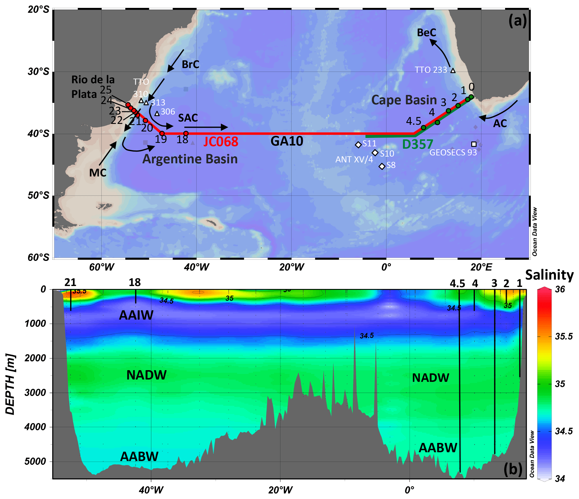
Figure 1(a) Map of cruise tracks, station locations and surface currents. GA10 cruise D357 and JC068 stations are labelled with green and red circles, respectively. Stations of previous Ra studies are labelled with open symbols (Transient Tracers in the Ocean (TTO): Key et al., 1990, 1992a, b; GEOSECS: Ku and Lin, 1976; ANT XV/4: Hanfland, 2002). Surface currents are shown with arrows. (b) Salinity profiles along the cruise track of UK GEOTRACES GA10 are labelled with water masses. Vertical lines indicate the stations where vertical Ra water profiles are available.
Oceanic mixing and advection facilitate the transport of nutrients to the euphotic zone (Oschlies, 2002). The distribution of TEs in the surface ocean is primarily controlled by the inputs from the continental shelves (i.e. rivers, submarine groundwater discharge (SGD), and sediments), deep ocean waters (regeneration, continental slopes, and hydrothermal vents) and aeolian inputs, with these mediated by lateral and vertical mixing (diffusive turbulent mixing), advection, particle scavenging and biological uptake. In particular, deep winter mixing has been shown to be an important mechanism bringing TEs from below the mixed layer to the surface ocean (Tagliabue et al., 2014; Achterberg et al., 2018, 2020; Rigby et al., 2020). Geochemical tracers for ocean mixing can therefore be used to indirectly estimate TE inputs and outputs in the upper ocean, e.g. tritium (3He) (Jenkins, 1988; Schlitzer, 2016) and radium isotopes (228Ra) (Cai et al., 2002; Ku et al., 1995; Nozaki and Yamamoto, 2001; Sarmiento et al., 1990; Moore, 2000; Charette et al., 2007; Sanial et al., 2018).
The four naturally occurring radium isotopes cover a wide range of half-lives (226Ra, years; 228Ra, years; 223Ra, d; 224Ra, d), which enables us to study oceanic processes at different timescales. Ra-228 is continuously produced through the decay of 232Th in shelf sediments, released into seawater, and then transported into the surface open ocean by mixing or advection. The half-life of 228Ra is much shorter than the estimated Ra residence time by removal of ∼500 years (Moore and Dymond, 1991). The distribution of 228Ra in the ocean is therefore mainly controlled by ocean transport and radioactive decay, and can be used to estimate lateral mixing from the coastal shelf or continental slope to the open ocean (Kaufman et al., 1973; Knauss et al., 1978; Yamada and Nozaki, 1986; Sanial et al., 2018). Subsequent downward mixing from the surface can also be used to assess vertical mixing in the upper water column (Charette et al., 2007; Sarmiento et al., 1976; van Beek et al., 2008). Radium-228 has also been used as a conservative tracer to estimate submarine groundwater discharge (SGD) (Windom et al., 2006; Moore et al., 2008; Kwon et al., 2014; Rodellas et al., 2015; Le Gland et al., 2017), river inputs (Vieira et al., 2020), continental shelf (Rutgers van der Loeff et al., 1995; Charette et al., 2016; Sanial et al., 2018; Kipp et al., 2018a) and hydrothermal inputs (Kipp et al., 2018b).
Previous work has assessed TE inputs to the wider South Atlantic from rivers (Vieira et al., 2020), atmospheric dust (Gaiero et al., 2013), shelf sediments (Graham et al., 2015), the Agulhas current (Paul et al., 2015) and hydrothermal vents (Saito et al., 2013). There are also studies of TE distributions and basin-scale inputs in some areas of the South Atlantic (e.g. Chever et al., 2010; Bown et al., 2011; Noble et al., 2012). Two UK GEOTRACES cruises in 2010–2012 provided a significant increase in such observations, focusing particularly on 40∘ S (Homoky et al., 2013; Browning et al., 2014; Wyatt et al., 2014, 2020; Chance et al., 2015; Menzel Barraqueta et al., 2019). These published studies did not assess the fluxes of TEs by ocean mixing and transport. In this study, we address this issue using samples taken on the two 40∘ S Atlantic UK GEOTRACES cruises. We investigate the distributions of 228Ra, as well as 226Ra, in both the Argentine and Cape basins of a 40∘ S latitudinal transect in the Atlantic Ocean. This is also the first exploration of the vertical and horizontal 228Ra distributions reported for the Cape Basin. We investigate the application of seawater 228Ra as a tracer for vertical and horizontal mixing in the surface South Atlantic, to provide estimates of the dissolved TE (dTE) fluxes, with a focus on cobalt, iron, and zinc, in the micronutrient-depleted euphotic zone.
2.1 Hydrographic setting
The study was conducted from the RRS Discovery and RRS James Cook during two UK GEOTRACES cruises, D357 and JC068, along the GA10 40∘ S transect of the Atlantic Ocean (Fig. 1). The surface currents show dynamic interaction and mixing on both the western and eastern sides of this transect. In the Argentine Basin, the Río de la Plata estuary is located on the western margin of the transect. The boundary Brazil Current (BrC) and Malvinas Current (MC) meet between 33 and 45∘ S along the continental margin of South America and these become the South Atlantic Current (SAC) transporting water eastwards along 40∘ S. The water from the BrC is captured between Stn20 and Stn21 with a strong west to east gradient in salinity and other chemical and physical properties, which also suggests a limited exchange of water across the continental shelf break (see below). In the Cape Basin, the SAC turns northeast before reaching the continent of Africa, and the Agulhas Current (AC) adds warm water eddies from the Indian Ocean. The warm and salty water of the AC was sampled in the top 500 m at Stn2 (Fig. 1b). These currents meet and become the Benguela Current (BeC) flowing through the Cape Basin and into the South Atlantic.
2.2 Water sampling
Seawater samples for Ra analysis were collected from 14 stations on the D357 and JC068 cruises (Fig. 1). The first cruise (D357) took place in the SE Atlantic (Cape Basin) between October and November 2010; the second cruise (JC068) took place along the whole 40∘ S transect between December 2011 and January 2012. For radium isotope analyses, the Cape Basin samples were only taken from D357, and the Argentine Basin samples were taken from JC068. For TEs, samples were taken from both D357 and JC068. Stations from these cruises are shown along with those from previous Ra studies (e.g. GEOSECS and TTO) in this region (Fig. 1a).
A total of 48 samples were analysed for 228Ra 226Ra ratio and 228Ra concentration, and 33 samples for 226Ra concentration, collected using three different sampling techniques during the cruise. Surface seawater samples (80–100 L) at 5 m depth were collected via a trace-metal clean seawater supply (fish) using a Teflon bellow pump (Almatec-A15) and acid-cleaned tubing. Samples between 50 and 400 m were collected using a standard conductivity, temperature, and depth (CTD) rosette, typically sampling from four 20 L Niskin bottles. These samples were stored briefly in low-density polyethylene (LDPE) cubitainers and then filtered through Mn-fibre cartridges by gravity (flow rate <0.5 L min−1) on board for the extraction of radium isotopes (Moore et al., 1985; Reid et al., 1979). In addition, large-volume seawater sampling (300–600 L) was carried out using in situ stand-alone pump (SAP) systems, pumping seawater over Mn fibres in polypropylene cartridges (van Beek et al., 2008) at flow rate of 2–5 L min−1 at three selected sampling stations (Stn1, Stn3, and Stn4.5). As the cartridge Ra collection efficiency varies hugely, ranging from 70 % to 128 % (Geibert et al., 2013), all samples collected by these collection techniques (pump, CTD, and SAP) were only used for measurement of 228Ra 226Ra ratios. To address the efficiency issue, for most samples, a separate sample of 250 mL seawater was also collected for measurement of 226Ra concentration. This method provides the advantage of allowing a correction for variable efficiencies during the sample preparation.
Trace element samples were collected using a titanium CTD rosette fitted with trace-metal clean Teflon-coated Niskin bottles and filtered on board through 0.8/0.2 µm polyethersulfone (PES) membrane cartridge filters (AcroPak500™, Pall) before analysis. All the TE data and fluxes reported and discussed in this study refer to the dissolved fraction only. The data of zinc and cobalt were measured and published by Wyatt et al. (2014, 2020). Some of the iron data were determined and published by Browning et al. (2014) and Clough et al. (2016). All the TE data are available on the GEOTRACES Intermediate Data Product (IDP) 2017 (Schlitzer et al., 2018).
All the trace-metal cleaning procedures followed the GEOTRACES sampling protocols (Cutter et al., 2010). In brief, the sample tubing and bottles were rinsed with Milli-Q water and filled with 0.1 M HCl for 1 d. After emptying the acid, the tubing and bottles were rinsed thoroughly with Milli-Q water. The tubing and bottles were also rinsed with open-ocean seawater before sampling.
2.3 Ra isotopes analysis
Mn-fibre samples were first counted on board using a four-channel radium delayed coincidence counting (RaDeCC) system for 224Ra, 223Ra, 228Th, and 227Ac (Moore and Arnold, 1996), but the data for 224Ra, 223Ra, 228Th, and 227Ac are not discussed in this paper. After the counting, Ra was purified using the following procedure for precisely measuring 228Ra 226Ra ratios and 228Ra concentrations by a Nu Instrument multi-collector inductively coupled plasma mass spectrometry (MC-ICP-MS) at the University of Oxford following the procedures established by Hsieh and Henderson (2011). Mn fibres were ashed at 550 ∘C for 6 h and then leached with distilled 6 N HCl to remove Ra from the ashed fibres. Ra was then co-precipitated with Sr(Ra)SO4 in the leached solution, centrifuged, and cleaned with 3 N HCl and pure H2O a few times until the pH was >4. To increase the dissolution rate, Sr(Ra)SO4 was converted to Sr(Ra)CO3 by adding 2 mL 1 M Na2CO3 solution and heated on a hotplate for 3 h. After centrifuging and discarding the supernatant, Sr(Ra)CO3 was finally dissolved in 2 mL 6 N HCl for ion exchange column chemistry, using Bio-Rad AG50-X8 cation exchange resin (to separate Ra and Ba from 228Th and other matrix elements, e.g. Ca, Sr, and Mn) and Eichrom Sr-Spec resin (to separate Ra from Ba to avoid molecular interferences during MC-ICP-MS analysis).
Smaller seawater samples (250 mL) collected for 226Ra were spiked with a 228Ra spike (Hsieh and Henderson, 2011) and the Ra was purified by the precipitation of CaCO3 and processing with ion exchange columns of AG1-X8, AG50-X8, and Sr-Spec resin for the measurement of 226Ra concentrations by MC-ICP-MS (Foster et al., 2004). In general, the contribution of seawater 228Ra (<0.05 attomole) is negligible, compared to the spiked 228Ra signal (≈70 attomole). Assessments of overall chemical blanks were conducted the same way as for the samples throughout the whole chemical procedures, except that there was no added seawater. The blanks were found to contribute less than 1 % of the 226Ra in the sample and were not detectable for 228Ra.
During the MC-ICP-MS analyses, 228Ra and 226Ra were measured simultaneously on two ion counters, and the uranium standard CRM-145 was used to bracket each sample for the mass bias and ion counter gain corrections. Instrumental memories of 228Ra and 226Ra were also detected on ion counters before each measurement. The machine memory was about 0.2±0.1 cps (counts per second) (n=16, 2 SE). The memory correction was insignificant for 226Ra, because the ratio of memory to sample signal is small (). However, the memory correction could be significant for samples with low 228Ra activities and count rates. For instance, the count rate during analysis of 228Ra on the sample collected at 4741 m at Stn4.5 was only 0.5 cps. At this low count rate, instrumental memory contributed ∼40 % of the signal to the sample 228Ra signal and the uncertainty of memory correction becomes substantial. In this study, most of the surface and deep waters in the South Atlantic were measured at count rates >2 cps 228Ra, which provides assurance that the contribution of the instrumental memory uncertainty to the total uncertainty is <10 %.
For samples without accompanied 226Ra measurements, silica data (Table 1) are used to assess 226Ra activities (Appendix A). The Atlantic Ocean 226Ra–Si relationship is based on the GEOTRACES (GA03), GEOSECS, and TTO datasets (Fig. A1 in Appendix A, Ku and Lin, 1976; Key et al., 1990, 1992a, b; Charette et al., 2015). This relationship is used to determine 226Ra activities in the 27 cases where no subsamples were collected for separate 226Ra analysis (such 226Ra estimates are shown in brackets in Table 1). The relationship has a slope of 0.119 dpm 100 L−1 of 226Ra per µmol L−1 of Si and an intercept of 8.8 dpm 100 L−1, which is comparable with the average slope of 0.1 observed by Broecker et al. (1976) in the Atlantic. The Si-extrapolated 226Ra and measured 226Ra activities (data from this study and the TTO) show a relatively consistent result although the extrapolated 226Ra has a larger uncertainty (±11 % 2 SE) than the measured 226Ra uncertainty (±4 %, 2 SE). The paired t test shows a p value of 0.55 (>0.05), suggesting that the differences between the extrapolated 226Ra and the measured 226Ra data are not statistically significant. The uncertainties of 226Ra activity have been used in the error propagation of 228Ra activity; the total uncertainty of 228Ra is typically about 6 %–12 % (2 SE).
Table 1226Ra and 228Ra activities, activity ratios, and silica concentration.
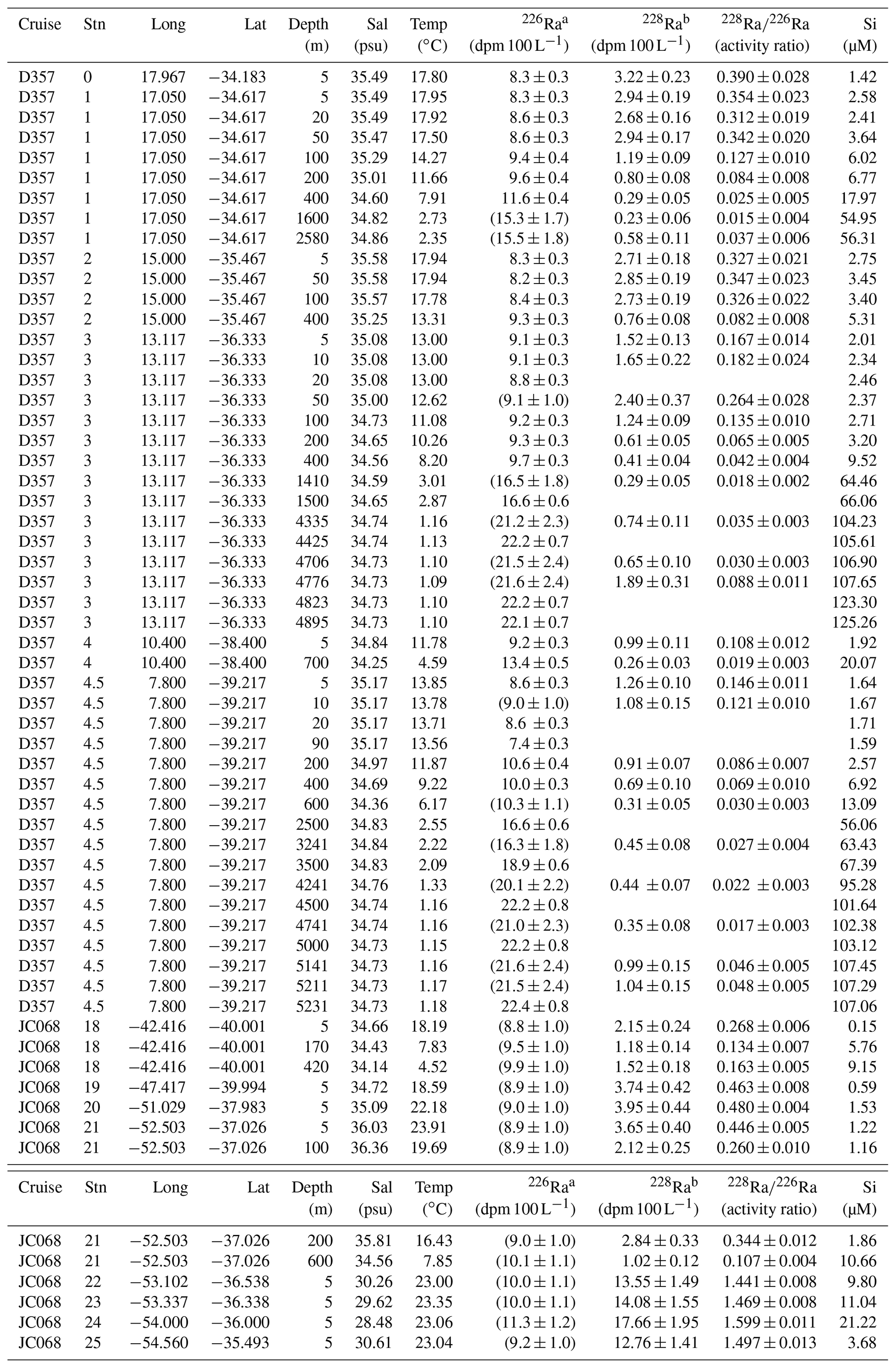
a Ra-226 activity in brackets is extrapolated from the 226Ra–silica relationship in Fig. A1. b Ra-228 activity is calculated from the activity ratio of multiplied by 226Ra activity. All errors are 2 standard errors.
2.4 228Ra-derived 1-D mixing models
The distribution of seawater 228Ra in the ocean is mainly controlled by mixing, advection, radioactive decay, and additional removal/input. It has been widely used as a tracer for measuring diffusion coefficients and advection rates on a basin-wide scale in the surface or at intermediate depths in the ocean (e.g. Cochran, 1992; Ku and Luo, 2008; Sanial et al., 2018). The one-dimensional (1-D) 228Ra advection–diffusion model is commonly expressed by the following formula (e.g. Moore, 2015):
where A is activity of 228Ra, t is time, Kx is horizontal eddy diffusion coefficient, w is advection velocity, x is offshore distance, λ is decay constant ( s−1), and J is additional input or removal of 228Ra.
To use the model to accurately calculate the mixing rates, several assumptions need to be made.
2.4.1 Steady state ()
This assumption requires long-term monitoring of 228Ra activities in the ocean due to the long half-life of 228Ra. Charette et al. (2015) compared the 228Ra data in the North Atlantic from the US GEOTRACES and the TTO programmes, and found that the upper ocean 228Ra inventories have remained constant over the past 30 years. Although 228Ra seasonality in coastal areas may introduce uncertainty to the mixing model, the assumption of steady state is likely to be valid for 228Ra on decadal timescales and at ocean basin scales. The comparison between our 228Ra data and the limited data from the TTO in this region shows good agreement (Fig. 2b), supporting this assumption for the South Atlantic.
2.4.2 No additional input or removal of 228Ra ()
Based on particle removal, Ra residence time is estimated to be ∼500 years in the surface ocean (Moore and Dymond, 1991). However, there is no measurable particle removal of Ra in the surface open ocean at the timescale of 228Ra half-life (5.75 years) (Moore, 2015). In theory, the distribution of seawater 228Ra is controlled by both vertical and horizontal mixing. For example, vertical mixing could potentially introduce additional “removal” of 228Ra from the surface water and affect the horizontal distribution of 228Ra in the surface ocean, which would require 2-D models and a high sample resolution dataset to resolve the problem. However, vertical mixing (∼ 0.1–1 cm2 s−1) is typically 5 to 8 orders of magnitude smaller than horizontal mixing (∼105–107 cm2 s−1), and the sample resolution is not good enough for precise 2-D modelling in this study. Therefore, we only apply the 1-D model to estimate the maximum horizontal mixing rates by neglecting the term of downward mixing.
Similar assumptions need to be made for the 228Ra-derived vertical mixing – the gradient of 228Ra with depth mainly reflects the vertical mixing rates, and the vertical 228Ra distribution is not affected by additional input of horizontal 228Ra below the mixed layer. These assumptions are mostly true in the upper open ocean, where horizonal 228Ra mainly comes from the continental margins (shelf and slope sediments) and there is a lack of other important 228Ra sources in the middle of the ocean. However, if the lateral input becomes important and starts to interfere with the 228Ra vertical profiles (e.g. receiving strong advective shelf water or profiles closer to the seafloor), the 1-D 228Ra-derived vertical mixing rates can be significantly overestimated.
2.4.3 Boundary conditions (A=A0 at x=0 and A=0 at x→∞)
It has been pointed out that the boundary condition of A=0 at x→∞ is incorrect for using 228Ra to determine coastal mixing as the distribution of 228Ra could be controlled by water mass mixing within the coastal distance scale (<50 km) rather than eddy diffusion (Moore, 2000). In theory, this boundary condition may be valid on the ocean basin scale, as the major sink of 228Ra in the ocean is radioactive decay. However, observed seawater 228Ra is still not completely zero in the remote ocean. To avoid this problem, we follow the suggestion of Moore (2015) and define the 228Ra excess (228Raex=228Ra − 228Rabg) by subtracting the background value in the middle of the South Atlantic, 228Rabg: 0.23±0.06 dpm 100 L−1 (1 SE, n=6). This value is determined by the average of the observed values at (1) the remote surface waters in a previous study around the 40∘ S transect (Hanfland, 2002; Fig. 1, ANT XV/4 station S8, S10, and S11); and (2) the water depth between 1000 and 3500 m in this study (except for 2580 m at Stn1 on the continental slope). The mid-depth 228Ra background (1000–3500 m) shares a similar background as the remote surface waters (∼0.2 dpm 100 L−1), suggesting that the 228Ra background needs to be corrected in both horizontal and vertical mixing calculations. For comparison, the central North Atlantic shows a similar mid-depth 228Ra background value (∼0.16 dpm 100 L−1) between 1000 and 3000 m depth from the GEOTRACES GA03 transect (Stn12–20; Charette et al., 2015). However, the surface value in the central North Atlantic (∼2.2 dpm 100 L−1) is significantly higher than that in the South Atlantic (∼0.2 dpm 100 L−1), which has also been observed by Moore et al. (2008). We therefore use a background value of 228Rabg: 0.23±0.06 dpm 100 L−1 determined from the South Atlantic.
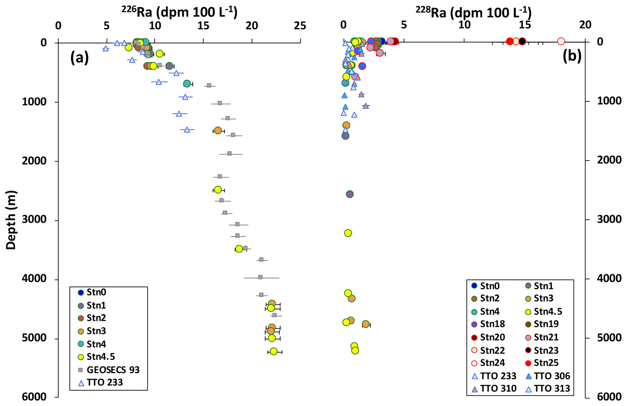
Figure 2Depth profiles of (a) 226Ra and (b) 228Ra activities. The grey squares show Ra data from the previous GEOSECS study (Ku and Lin, 1976); the triangles show Ra data from the TTO programme (Key et al., 1990, 1992a, b). Different water masses are characterised in the (a) 226Ra profile (see details in text). Error bars are ±2 SE.
The boundary condition can now be rewritten as at x=0 and Aex=0 at x=∞. Considering the assumptions discussed above, Eq. (1) can be written as
In this study, we consider two scenarios in the horizontal 228Ra calculations: (1) mixing only (w=0) and (2) advection only (Kx=0). We use these two scenarios to provide independent assessments of chemical fluxes in the surface ocean, to bracket the range of possible TE fluxes that are consistent with the 228Ra data regardless of the combination of mixing and advection in the real ocean. The advection model is only applied to the Argentine Basin data after the shelf break where the advection signal is strong because of the Brazil Current. Although the advection only scenario is an unrealistic one, it provides an end-member for comparisons of TE fluxes under different settings. Using the boundary conditions, at x=0 and Aex=0 at x=∞, Eq. (2) can be solved for diffusive mixing only:
and for advection only:
where Aex_0 is the activity of 228Raex at x=0 (i.e. Stn0 or Stn25); is the distance at which Aex=0.5Aex_0; and is the half-life of 228Ra (5.75 years). The exponential fit of the surface 228Ra data provides the estimate of the maximum diffusion coefficients (Kx) at both ends of the transect, and the linear fit of the surface 228Ra data after the shelf break in the Argentine Basin provides the minimum estimate of the advection water transport (w) along the west end of the transect (see discussion below).
For vertical mixing, the calculation of Kz is based on a situation in which 228Ra is mixed horizontally away from the coast in the surface mixed layer and then down into the subsurface. The 1-D mixing model can therefore be applied to the depth profiles of 228Ra to calculate Kz near the surface ocean. Under similar boundary conditions at z=0 and Aez=0 at z=∞, the diffusion equation can be solved for vertical mixing to fit the vertical 228Ra profiles:
where Aez_0 is the activity of 228Raex at z=0 (i.e. the mixed layer). In the 1-D mixing model, the term for diapycnal advection is generally negligible, as the oceanic vertical advection velocity is usually very small, i.e. 10−3–10−5 cm s−1 (Liang et al., 2017).
2.5 Trace element flux calculations
In this study, we use three different 228Ra approaches to quantify the horizontal and diffusive vertical dTE fluxes in the Cape Basin and Argentine. More details of the calculations are provided in Appendix D.
2.5.1 228Ra-derived diffusive TE fluxes
To calculate both lateral and vertical TE fluxes, the 228Ra-derived diffusion coefficients (Kz or Kx) are applied to Fick's first law of molecular diffusion in the following equation:
where FTE−d is the diffusive flux of the TEs, and or Δz is the gradient of TE concentration over either the horizontal distance x to the coasts or the vertical depth z below the mixed layer, which can be obtained from the linear regression of horizontal and vertical TE profiles (Sect. 3.2).
2.5.2 228Ra-derived advective TE fluxes
Surface water after the boundary of the shelf break and the Brazil Current in the Argentine Basin carries strong offshore advection signals along the SAC towards the open ocean (Fig. 1). Assuming that the mixing of TE is conservative, the advective TE fluxes can be calculated using the following equation:
where FTE−a is the offshore advective flux of TE, w is the net offshore advection velocity along the SAC in the Argentine Basin, and [TE]ave−0 is the average concentrations of dissolved TEs in the initial advective waters around where the Brazil Current merges into the SAC (around Stn21).
2.5.3 Ra-ratio-derived TE fluxes
Previous studies have combined the use of the shelf 228Ra fluxes with the ratios of Ra in the surface waters between continental shelves and open oceans to estimate the shelf–ocean TE inputs from the continental margins to the open oceans (Charette et al., 2016; Sanial et al., 2018; Vieira et al., 2020). This method provides the integrated net fluxes of TEs, considering all the possible inputs (e.g. rivers, SGD, and sediments) and outputs (e.g. particle scavenging, biological uptake, and radioactive decay) of 228Ra and TEs during water mixing between the continental shelf and the open ocean. More details of the method are given in Charette et al. (2016). In brief, assuming that the net shelf–ocean exchange is mainly driven by eddy diffusion, the cross-shelf TE fluxes can be calculated using the following equation:
where F228Ra is the cross-shelf 228Ra flux (Appendix D); TEshelf and 228Rashelf are the average concentrations of the TE and 228Ra in the surface waters on the shelf (GA10W: between Stn23 and Stn25; GA10E: between Stn0 and Stn1), respectively; and TEoecan and 228Raocean are the average concentrations in the open ocean (GA10W: between Stn18 and Stn19; GA10E: between Stn4 and Stn4.5). The ratios of Ra are reported in Table D1 in Appendix D.
3.1 Ra isotope concentrations
The results of 226Ra and 228Ra activities and the activity ratios of 228Ra 226Ra are presented in Table 1 (with ±2 SE). The vertical profiles of measured 226Ra show good agreement with the data from the closest GEOSECS and TTO stations in this region (e.g. Ku and Lin, 1976; Key et al., 1990, 1992a, b) (Fig. 2a). Ra-226 activities range from 8.2 to 22.4 dpm 100 L−1. In this study, the results of 226Ra are mainly used for calculating 228Ra activities, and will not be discussed in further detail.
The activity ratios of 228Ra 226Ra range from 0.017 to 1.599 in the surface water and are comparable with the ratios from 0.080 to 2.810 observed in previous studies in this region (TTO data, Windom et al., 2006; Hanfland, 2002). The vertical profiles of 228Ra activity are shown in Fig. 2b. In surface waters, the activities of 228Ra ranging from 1.02 to 17.66 dpm 100 L−1 in the Argentine Basin are consistent with the observed values from 0.07 to 24.0 dpm 100 L−1 from the previous studies (TTO data and Windom et al., 2006), and the activities of 228Ra ranging from 0.99 to 3.22 dpm 100 L−1 in the Cape Basin are consistent with the observed values from 0.67 to 4.23 dpm 100 L−1 from the previous study (Hanfland, 2002). Between 600 and 4000 m, 228Ra 226Ra ratios decrease to 0.015–0.030 and 228Ra activities decrease to 0.29–0.32 dpm 100 L−1. In the 100 m closest to the ocean floor, the ratios of 228Ra 226Ra increase to 0.048–0.088 and the activities of 228Ra also increase to 1.07–1.94 dpm 100 L−1. This is the first dataset of seawater 228Ra reported in the intermediate and deep waters in the Cape Basin. The 228Ra values in the Cape Basin are noticeably higher than those observed in intermediate (< 0.1 dpm 100 L−1) and deep waters (0.22–0.28 dpm 100 L−1) to the south in the Southern Ocean (Charette et al., 2007; van Beek et al., 2008). The vertical profiles of seawater 228Ra in the Cape Basin are consistent with GEOSECS and TTO observations elsewhere in the South Atlantic Ocean (Moore et al., 1985). The samples collected by pump (fish), CTD, and SAP within the mixed layer at each station show consistent 228Ra and 226Ra results, suggesting that there is no significant difference in the Ra results between these three sampling methods.
3.2 Micronutrient concentrations
Dissolved Co, Fe, and Zn concentration data (Wyatt et al., 2014, 2020; Browning et al., 2014; Clough et al., 2016; Schlitzer et al., 2018) are summarised in Appendix B (Tables B1 and B2). At the continental margins, surface shelf waters show much higher trace element concentrations (Co: 146.2 pM, Fe: 1.53 nM, and Zn: 0.59 nM in the Argentine Basin margin; Co: 46.9 pM, Fe: 0.35 nM, and Zn: 0.14 nM in the Cape Basin margin) than observed in the open-ocean surface waters along the 40∘ S transect (Fig. 3). In the Argentine Basin, the distribution of trace elements generally follows the salinity in the surface waters. The low-salinity waters (<29 psu) around 200 km from the South America coast show high TE concentrations (Co: >80 pM, Fe: >1 nM, and Zn: >0.5 nM). In contrast, the high-salinity waters (>35 psu) in the Brazil Current show much lower TE concentrations (Co: <60 pM, Fe: <0.5 nM, and Zn: <0.2 nM). Similar correlations between trace elements and salinity have been observed along other western boundaries of the Atlantic as well (e.g. the North American shelf; Bruland and Franks, 1983; Noble et al., 2017). In the upper ocean (<600 m), these trace element concentrations are generally low in the surface mixed layer and increase with depth below the mixed layer (Fig. 4). Co concentrations range from 1.6 to 61.2 pM, and Fe and Zn concentrations range from 0.05 to 0.54 and 0.01 to 0.53 nM, respectively. In general, these trace element concentrations (<600 m) are slightly higher in Stn1 than other stations further away from the continental shelf.

Figure 3Dissolved trace elements (dCo, dFe, and dZn) and salinity in the surface water (<10 m) along the 40∘ S Argentine and Cape Basin transects. Red squares show data from cruise JC068, and green circles show data from cruise D357. The orange band indicates the boundary of the BrC in the Argentine Basin transect, highlighted by high salinity and changing TE gradients. [TE]ave−0 is the average concentrations of dissolved TEs in the initial advective waters around where the Brazil Current merges into the SAC (around Stn21; ±1 SD, n=4). The dashed lines show linear regression trends through the TE data (Argentine Basin transect: only data from the shelf to BrC; Cape Basin transect: the whole transect), and the gradient () errors are ±1 SD.
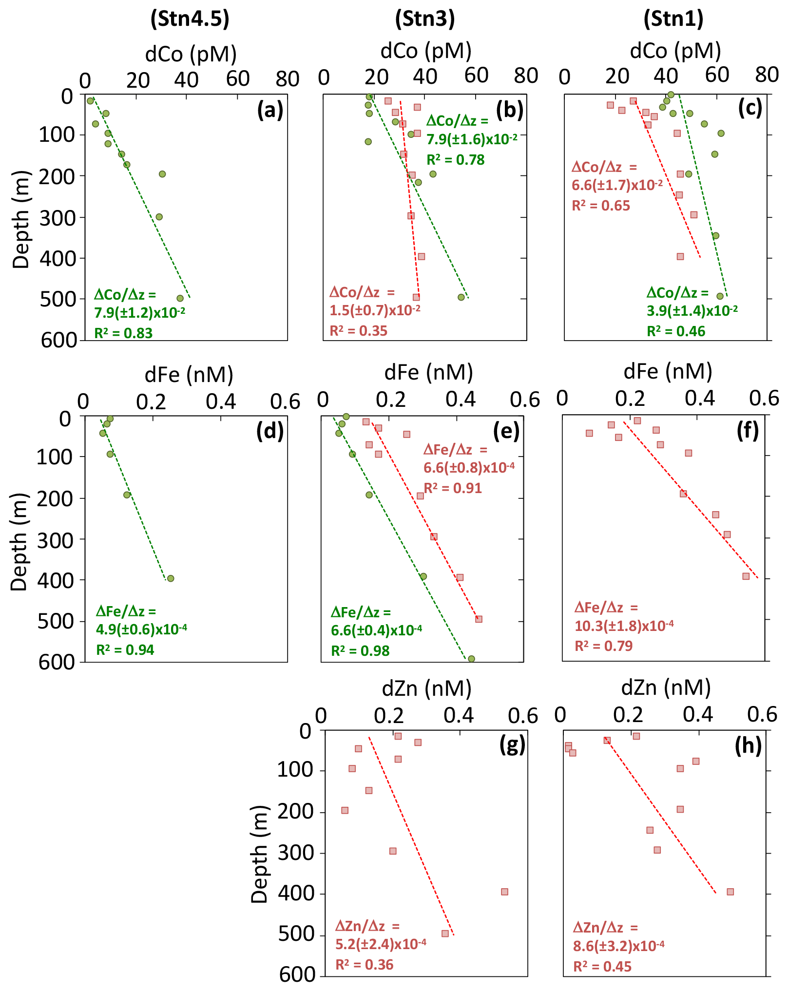
Figure 4Depth profiles of dissolved trace elements (dCo, dFe, and dZn) in the upper ocean (<600 m). Red squares show data from cruise JC068, and green circles show data from cruise D357. The dashed lines show linear regression trends, and the vertical gradient () errors are ±1 SD.
4.1 228Ra-derived horizontal mixing and advection
4.1.1 Argentine Basin
The distribution of 228Raex in the Argentine Basin (GA10W) is controlled by the Rio de la Plata river plume and the Brazil Current (Fig. 5a), and this is supported by a good correlation with salinity (linear regression R2=0.96; Fig. C1 in Appendix C). If we apply the 1-D mixing model (Eq. 3) to fit the 228Raex data between Stn25 and Stn21, across the boundary of the Brazil Current, the gradient of the exponential fit (a) is 0.0047±0.0027 and the estimate of the offshore horizontal diffusion coefficient Kx is cm2 s−1, which is likely to be an overestimate due to the influence of the river plume and the advection of the boundary current. Nevertheless, this estimate is still within the range of other estimates of Kx between 105 and 108 cm2 s−1 in a variety of margin and open-ocean settings (e.g. Kaufman et al., 1973; Knauss et al., 1978; Yamada and Nozaki, 1986).
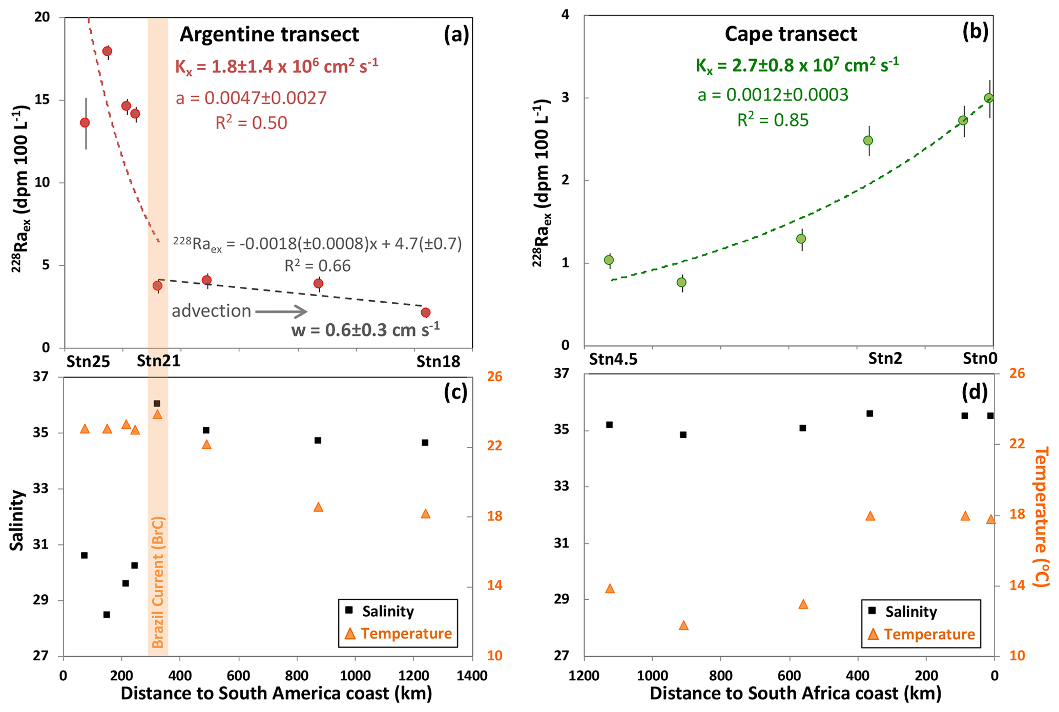
Figure 5Plots of 228Raex in the surface ocean (<10 m) along the (a) Argentine and (b) Cape Basin 40∘ S Atlantic transects, with the distributions of salinity and temperature shown in panels (c) and (d). The orange band indicates the boundary of the BrC in the Argentine Basin transect, highlighted by high salinity and temperature. The dashed red and green lines show exponential regression trends through the 228Raex data (Argentine Basin transect: only to BrC; Cape Basin transect: the whole transect). The gradients of the exponential fit (the a values) are used in Eq. (3) for the Kx calculation. The errors of a and Kx are ±1 SD. The dashed grey line shows a linear regression trend through the 228Raex data from BrC to the open ocean in the Argentine Basin transect, which is used in Eq. (4) to estimate the advection water transport velocity (w).
Across the boundary of the Brazil Current, the advection of the eastward flowing SAC shows a significant impact on the distribution of 228Raex in the surface Argentine Basin (Fig. 5a). If we apply the 1-D advection model (Eq. 4) to fit the data between Stn21 and Stn18 (Fig. 5a), the is 1116±600 km (from Stn 21) and the estimate of average advection velocity w is 0.6±0.3 cm s−1. Although the 228Ra-derived velocity is smaller than the typical velocities (2–4 cm s−1) around the South Atlantic subtropical gyre (Schlitzer, 1996), similar advective 228Ra signals have been previously observed in other surface ocean current systems, including the Peru and Kuroshio currents in the Pacific (Knauss et al., 1978; Yamada and Nozaki, 1986).
4.1.2 Cape Basin
Ra-228 data from the Cape Basin transect (GA10E) are used to calculate the offshore horizontal diffusion coefficient (Kx) in the Cape Basin (Fig. 5b). Applying the simple 1-D mixing model, assuming w=0, to fit the surface 228Raex data in the Cape Basin (Fig. 5b), the gradient of the exponential fit (a) is 0.0012±0.0003 and the estimate of Kx is cm2 s−1, which is an order of magnitude higher than the value observed in the Argentine Basin (see above) but within the range of other observed values in the oceans (105–108 cm2 s−1).
The horizontal diffusion coefficient Kx is likely to be overestimated in the Cape Basin due to the influence of episodic water advection. The Agulhas Current leakage (ACL) is known for transporting water from the Indian Ocean into the South Atlantic and episodically introduces eddies (Agulhas rings) into the Cape Basin (Beal et al., 2011). However, the signals of mixing and advection cannot be easily separated with the 228Ra data alone (Fig. 5b). For example, the distribution of 228Raex in the surface Cape Basin shows elevated values (Stn2 and Stn4.5) above the fitted curve and coincides with the elevated salinity and temperature data (Fig. 5d), which indicates that the elevated 228Raex is likely to come from an advective signal (e.g. ACL). The ACL signal has also been identified with a distinct Pb isotope signature in the upper water column at Stn2 (Paul et al., 2015). The application of a 1-D mixing model may actually be biased by the addition of these high 228Raex waters; therefore, the horizontal diffusion coefficient Kx is likely to be a maximum estimate for the Cape Basin. Nevertheless, the overall gradient of 228Raex, decreasing along the distance away from the shore, is driven by the loss of 228Ra through both water mixing and radioactive decay.
Despite uncertainty in the diffusion coefficients due to advection of other sources, the 228Ra data do place bounds on maximum horizontal mixing in the surface ocean away from the eastern and western boundaries of the Atlantic at 40∘ S. These bounds can be used to quantify the trace element inputs from the continental margins to the South Atlantic (see Sect. 4.3).
4.2 228Ra-derived vertical mixing
Vertical diffusion coefficients (Kz) are calculated at six stations where the depth profiles of 228Raex are available (Stn1, Stn2, Stn3, Stn4.5, Stn18, and Stn21). The best-fit exponential curve gradients (a) from the depth (z) profiles of 228Raex activities below the surface mixed layer are used in the same 1-D mixing model (Eq. 5) to calculate the vertical mixing coefficient Kz for the upper ≈600 m of each station in both the Argentine and Cape basins (Fig. 6), and resulting Kz values range from 1 to 53 cm2 s−1 at these stations. It should be noted that Stn2 only has one Ra data point below the mixed layer, and hence it is not considered in the vertical TE input calculations (Sect. 4.3), but the estimate of Kz shows a similar value as other stations with more data points. The high Kz values of 53 cm2 s−1 and 7 cm2 s−1 at Stn18 and Stn21, respectively, are most likely biased by the lateral inputs of 228Ra below the mixed layer (see later discussion). Excluding the values of Stn18 and Stn21, the range of Kz values from 1.0 to 1.7 cm2 s−1 is broadly comparable to the average Kz of 1.5 cm2 s−1 assessed from tritium measurements in the South Atlantic (Li et al., 1984). These estimates are also consistent with the range of observed vertical mixing from 0.1 to 10 cm2 s−1 using different methods (e.g. 7Be, SF6 dye release and microstructure shear probe methods) in different ocean basin settings (Kunze and Sanford, 1996; Ledwell et al., 1993; Martin et al., 2010; Painter et al., 2014; Kadko et al., 2020).

Figure 6Depth profiles of (a–f) seawater 228Raex activity in red (Argentine Basin) and green (Cape Basin) circles and density (sigma-t) shown in dashed grey lines, and (g–i) density and temperature in the upper ocean shown at Stn1, 2, 3, 4.5, 18, and 21. Depths of the mixed layer are labelled with the horizontal dashed orange lines, defined by the sigma-t and temperature profiles. The dashed red and green lines show exponential regression trends through the 228Raex data below the mixed layer (including the average value of the mixed layer). The gradients of the exponential fit (the a values) are used in Eq. (5) for the Kz calculation (errors ±1 SD).
Given that the calculation of Kz is based on the vertical gradients of 228Ra driven by vertical mixing and radioactive decay only, it therefore relies on the assumption that the vertical gradients are not dominated by lateral input of 228Ra at depths below the surface mixed layer. This assumption is supported by an inspection of horizontal 228Ra gradients at depths below the mixed layer (Fig. 7). Due to the sample resolution, detailed inspection is only available for the Cape Basin. Here, unlike the exponential change seen in the surface layer, 228Raex activities at 50 m and deeper do not show an increasing gradient towards the continental margin. This therefore argues against lateral mixing away from the shore as the major mechanism driving subsurface 228Ra concentrations in the Cape Basin. In addition, the distribution of 228Ra on an isopycnal surface (≈200 m depth) is largely constant and shows no lateral gradient (Fig. 7). Studies using theoretical models to simulate seawater 228Ra distribution have also shown that the horizontal eddy mixing (Kx) has little effect on the vertical distribution of 228Ra (Lamontagne and Webster, 2019).
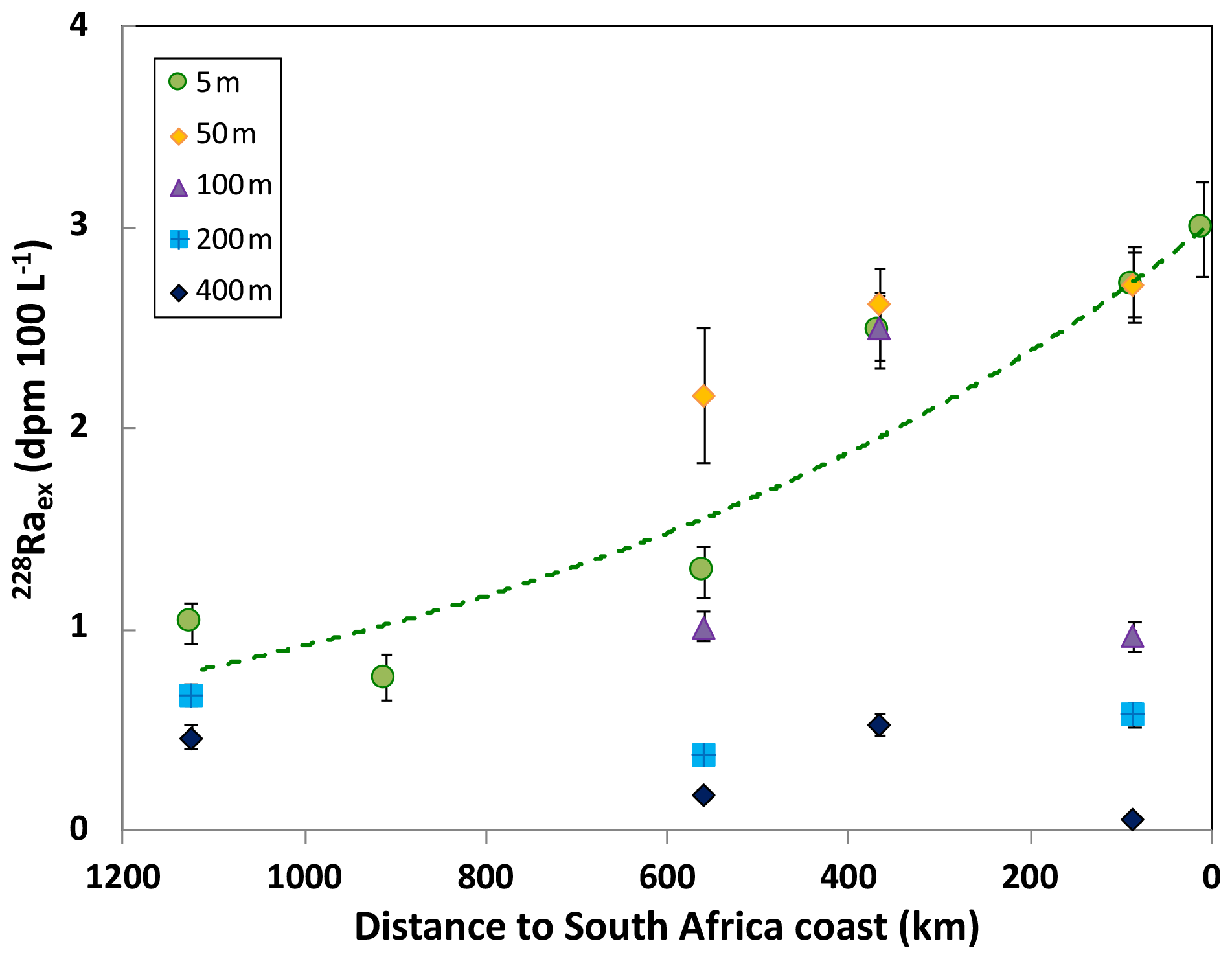
Figure 7Plots of 228Raex activity at water depths of 5, 50, 100, 200, and 400 m versus distance to the coast of Cape Town in South Africa. The dashed line shows an exponential regression line through the data at 5 m.
The depth profiles of 228Raex in the Argentine Basin show evidence of advective 228Ra below the mixed layer, potentially from the nearer-shore shelf waters. For example, elevated 228Raex values are seen around 400 m at Stn18 and 200 m at Stn21 (Fig. 6a and b) and these may explain the extremely high Kz values at these stations. Although the possibility of lateral inputs cannot be entirely excluded, particularly in the Argentine Basin, the vertical variation of 228Ra near the surface mixed layer still provides the first estimates of maximum vertical mixing and the upper limits of trace element inputs from vertical mixing to the surface ocean along the 40∘ S transect.
4.3 Trace element inputs in the South Atlantic
TEs are important micronutrients for marine productivity in the surface ocean. Atmospheric dust deposition is an important source of TEs to the surface ocean. The soluble atmospheric dust deposition fluxes to the surface 40∘ S Atlantic transect have been assessed from the same cruise as this study: these are 0.02–0.05 nmol Co m−2 d−1, 1.6–5.2 nmol Fe m−2 d−1 and 0.6–6 nmol Zn m−2 d−1 (Chance et al., 2015). However, other inputs of these TEs to the euphotic zone in the South Atlantic are still unknown (e.g. shelf–ocean and vertical mixing). In this study, we consider three different 228Ra approaches to quantify the horizontal and vertical TE fluxes in the Cape Basin and Argentine Basin along the 40∘ S transect: (1) 228Ra-derived diffusive, (2) 228Ra-derived advective, and (3) -ratio-derived TE fluxes (Sect. 2.5 and Appendix D). The results of the TE fluxes are summarised in Table 2 (shelf–ocean, horizontal) and Table 3 (vertical). For comparison, the horizontal TE fluxes are normalised to the areas of shelf–ocean cross section (Table D2; Urien and Ewing, 1974; Nelson et al., 1998; Emery, 1966; Windom et al., 2006; Carr and Botha, 2012; Hooker et al., 2013; Vieira et al., 2020) (illustrated in Fig. 8) unless otherwise specified.
Table 2228Ra-derived shelf–ocean dTE fluxes along the 40∘ S Atlantic transect*.

* Fluxes are normalised to the area of the cross-shelf section. All errors are ± 1 SD.
Table 3228Ra-derived vertical dTE fluxes along the 40∘ S Atlantic transect*.
* Fluxes are normalised to the surface area. All errors are ±1 SD.
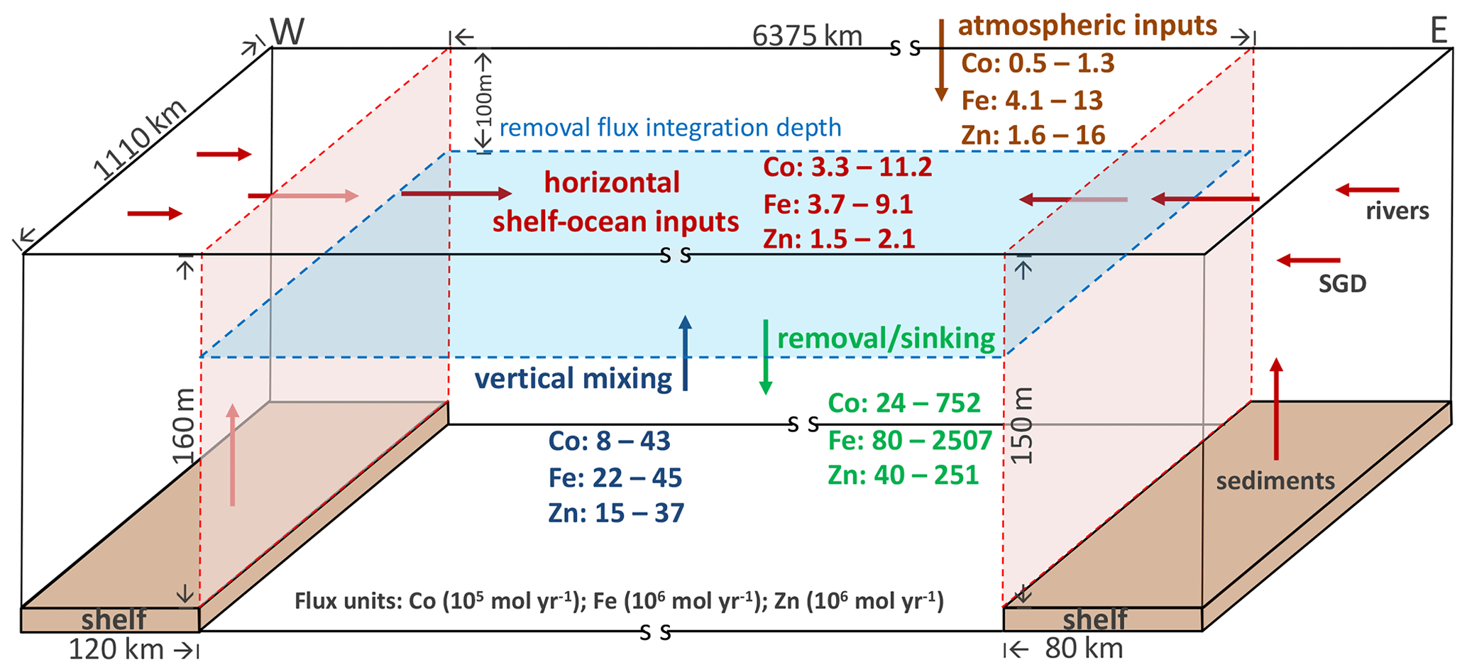
Figure 8Schematic diagram of dissolved trace element inputs and outputs in the high-productivity zone in the open ocean along the surface 40∘ S Atlantic transect. The approximate dimensions of the high-productivity zone and continental shelves are labelled, assuming that the zone spans across the latitude from 35 to 45∘ S (∼1110 km) and the longitude from 55∘ W to 20∘ E (∼6375 km) with a removal flux integration depth of 100 m. The arrows indicate different TE inputs and outputs in this region. The TE fluxes from Table 4 are shown and colour coded according to the sources. The vertical red cross sections are used to normalise the shelf–ocean TE and 228Ra fluxes. The net shelf–ocean TE fluxes represent the total inputs from rivers, SGD, and shelf sediments, and the outputs by particle or biological removal between the shelf–ocean mixing from both sides of the continental margins. The blue surface area is used to estimate the net TE inputs from dust and vertical mixing, and the red cross section above the mixed layer is used to estimate the net shelf–ocean TE fluxes (Table 4).
Surprisingly, the estimates of shelf–ocean TE fluxes show relatively good agreements (within uncertainties) between these three approaches (Table 2), given the limitations of the 1-D 228Ra-mixing model (Moore, 2015). A similar observation has also been found in the 228Ra study in the Peruvian continental shelf (Sanial et al., 2018), which suggests that the assumptions made for the 1-D 228Ra-mixing model are reasonable. In addition, the TE fluxes show consistent results between the D357 and JC068 data in the Cape Basin. These observations are likely to be a result of the gradients of 228Ra and TEs representing a long-term average at an ocean basin scale and being closer to a steady-state condition in the upper water column (e.g. the 228Ra and TEs in the North Atlantic; Charette et al., 2015).
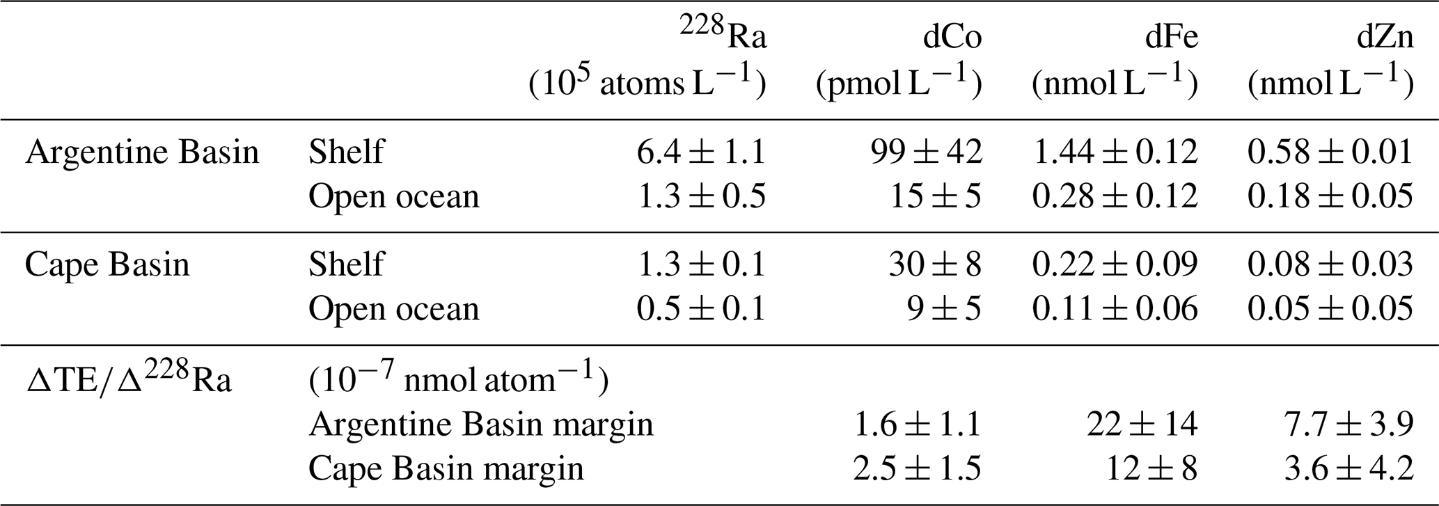
The 228Ra-derived shelf–ocean Co fluxes range from 4 to 21×103 nmol m−2 d−1 in the Argentine Basin margin and from 4.3 to 6.2×10³ nmol m−2 d−1 in the Cape Basin margin of the 40∘ S transect in the South Atlantic. In comparison, previous studies have applied the approach to estimate the shelf Co fluxes in several continental margins: the western North Atlantic (1.6×10⁵ nmol m−2 d−1; Charette et al., 2016), the Peruvian shelf (1.4×10⁵ nmol m−2 d−1, Sanial et al., 2018) and the Congo offshelf 3∘ S (2.8×10⁶ nmol m−2 d−1; Vieira et al., 2020). Although these fluxes are about 1 and 2 orders of magnitude, respectively, higher than the estimates in the South Atlantic, these regions are also associated with low oxygen which increases dissolution of Mn and Fe oxides in sediments and is prone to result in higher Co fluxes (e.g. Hawco et al., 2016). A low shelf–ocean Co flux has been reported in the eastern South Atlantic continental shelf (11–18×103 nmol m−2 d−1; Bown et al., 2011), which is very close to this study region in the Cape Basin.
Along the 40∘ S transect, the 228Ra-derived shelf–ocean Fe fluxes range from 8 to 19×104 nmol m−2 d−1 in the Argentine Basin margin and from 1.2 to 3.1×10⁴ nmol m−2 d−1 in the Cape Basin margin, which are slightly lower than the estimates of the shelf–ocean Fe flux (4.5×10⁵ nmol m−2 d−1) in the western North Atlantic (Charette et al., 2016). However, these fluxes are significantly lower than those high Fe fluxes observed in regions with river plumes (e.g. Congo River; 4.1×10⁸ nmol m−2 d−1; Vieira et al., 2020), submarine groundwater discharge (1.3×10⁸ nmol m−2 d−1, Windom et al., 2006) and the oxygen minimum zone (2.1×10⁶ nmol m−2 d−1, Sanial et al., 2018).
Lastly, the 228Ra-derived shelf–ocean Zn fluxes range from 2.7 to 6.3×10⁴ nmol m−2 d−1 in the Argentine and from 0.9 to 1.2×10⁴ nmol m−2 d−1 in the Cape Basin margins. When compared with the only available shelf–ocean Zn flux value (1.8×10⁶ nmol m−2 d−1) in the western North Atlantic (Charette et al., 2016), the Zn fluxes from this study indicate low Zn inputs in the South Atlantic. The different shelf–ocean Zn inputs between the North and South Atlantic require more detailed study to understand the processes supplying and removing Zn in the shelf waters and the influence of anthropogenic Zn. Nevertheless, the low Zn inputs support the previous observation that surface water along the 40∘ S transect has some of the lowest reported dissolved Zn concentrations in the global oceans (Wyatt et al., 2014).
From below the mixed layer, the vertical dissolved TE fluxes range from 0.1 to 1.2 nmol Co m−2 d−1, from 6 to 9 nmol Fe m−2 d−1, and from 5 to 7 nmol Zn m−2 d−1 along the 40∘ S transect (Table 3). These fluxes are consistent with previous estimates of Co in the South Atlantic (0.04–0.46 nmol m−2 d−1, Bown et al., 2011; 0.1–4 nmol m−2 d−1, Rigby et al., 2020) and in the high-latitude North Atlantic (0.15–0.5 nmol m−2 d−1, Achterberg et al., 2020), of Fe in the North Atlantic (0.14–21.1 nmol m−2 d−1; Painter et al., 2014), South Atlantic (1–27 nmol m−2 d−1; Rigby et al., 2020), and the Southern Ocean (3–31 nmol m−2 d−1, Blain et al., 2007; 2.3–14 nmol m−2 d−1, Charette et al., 2007), and of Zn in the Atlantic (2.7–137 nmol m−2 d−1, Rigby et al., 2020; Achterberg et al., 2020). However, the vertical diffusive Fe fluxes are smaller than some other vertical fluxes estimated in the Southern Ocean (27–135 nmol m−2 d−1; Dulaiova et al., 2009) and the winter mixing fluxes in the high-latitude North Atlantic (e.g. 27.3–103 nmol m−2 d−1; Achterberg et al., 2018). It is also worth mentioning that the TE fluxes estimated by Blain et al. (2007), Bown et al. (2011), and Painter et al. (2014) use the Kz values derived from the vertical density profiles instead of 228Ra.
4.4 Mass-balance budgets for trace elements in the South Atlantic
The mass-balance budgets of dissolved TEs from different sources (horizontal shelf inputs, vertical upward mixing, and atmospheric dust deposition) and sinks (exported fluxes) in the surface South Atlantic (40∘ S transect) are calculated and summarised in Table 4 and Fig. 8. The vertical upward mixing appears to be a more important source supplying TEs to the surface water at 40∘ S compared to atmospheric dust and continental shelf inputs. However, the dominant source or seasonal variation of the vertical TE inputs cannot be identified in this study. Apart from the internal regeneration, TEs from a subsurface lateral input from the continental margin can subsequently be brought to the surface by vertical mixing (e.g. Rijkenberg et al., 2014). Deep winter convective mixing has also been shown as an important source of TEs to the surface ocean (e.g. Achterberg et al., 2018, 2020; Rigby et al., 2020).
Table 4Net dTE fluxes in the 40∘ S Atlantic open-ocean high-productivity zone*.
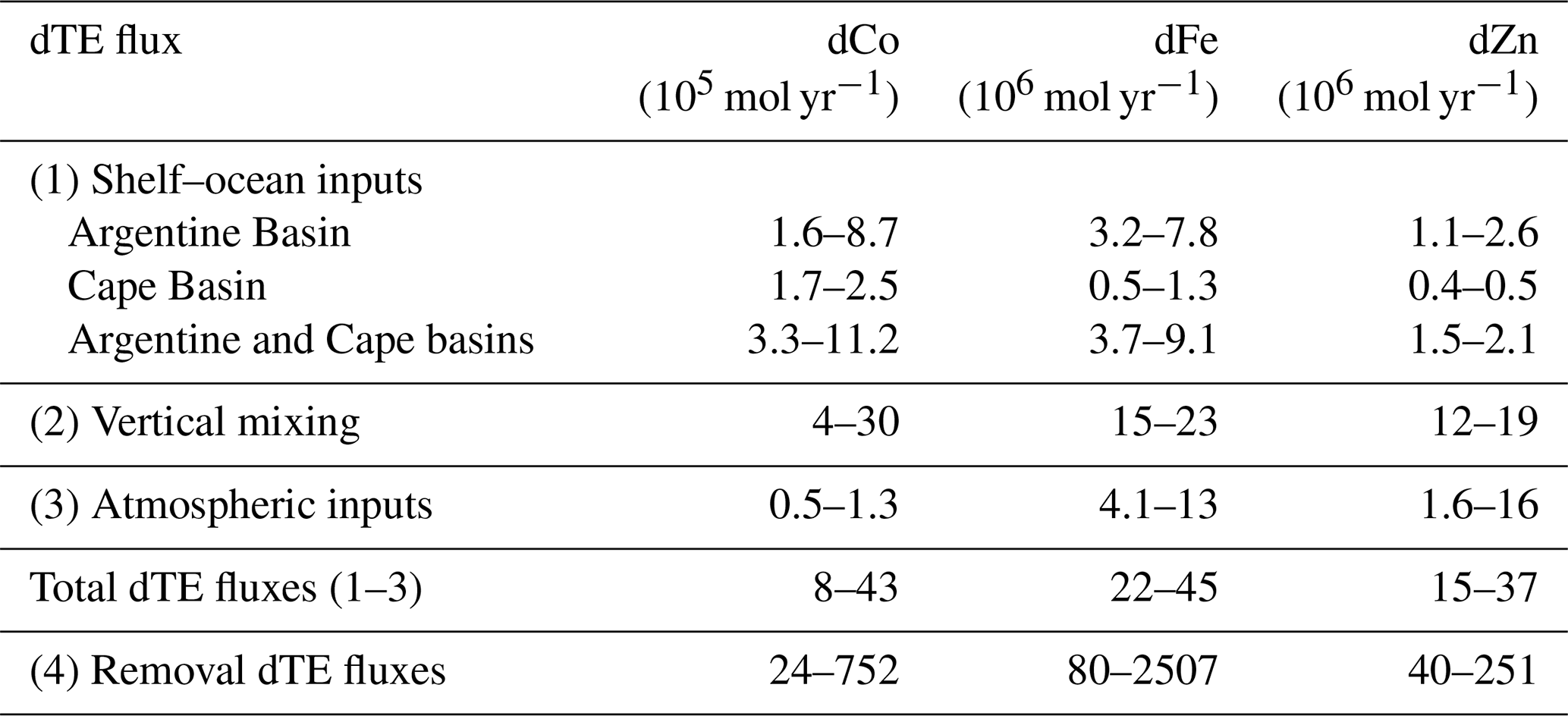
* The high-productivity zone is illustrated in Fig. 8. The net dTE fluxes of (1) shelf–ocean inputs (Table 2) are multiplied by the area of cross-shelf section above the removal flux integration depth (100 m). The net TE fluxes of (2) vertical mixing (Table 3), (3) atmospheric inputs (Chance et al., 2015), and (4) the exported fluxes (assessed from the 234Th–POC fluxes and ratios) are multiplied by the surface area.
A bulk estimate of the dissolved TE exported fluxes from the surface ocean, supported by new production biological uptake, can be made using a sinking particulate organic carbon (POC) flux and an estimated uptake ratio. In this study region, previous studies have reported the 234Th-derived POC fluxes ranging from 3.1 to 9.7 mmol C m−2 d−1 in the top 100 m integration depth (7.0±2.2 mmol C m−2 d−1; Thomalla et al., 2006; 6.4±3.3 mmol C m−2 d−1; Owens et al., 2015). The estimates of cellular ratios are 0.3–3, 10–100, and 5–10 µmol mol−1 for Co C, Fe C, and Zn C, respectively, based on the measurements in marine phytoplankton under different TE concentrations in surface waters (e.g. Co: 10−12 to 10−11 mol L−1, Sunda and Huntsman, 1995; Fe: 10−8 to 10−7 mol L−1, Sunda and Huntsman, 1997; Zn: 10−11 to 10−10 mol L−1, Sunda and Huntsman, 2000). These concentrations were chosen to represent the ranges of TE concentrations found in the surface waters of this region. Multiplying the POC fluxes with the ratios, the exported fluxes of Co, Fe, and Zn are 1–29, 31–970, and 16–97 nmol m−2 d−1, respectively. The results agree with the estimates of particulate TE removal fluxes in the North Atlantic (e.g. Co: 0.27–6.8 and Fe: 274–2740 nmol m−2 d−1; Hayes et al., 2018), even though the North Atlantic assessments have accounted for both biological uptake and particle scavenging fluxes by directly using TE 234Th ratios.
In general, the exported TE fluxes are higher than the net dissolved TE inputs that we have identified in this study (Table 4). Taking Fe as an example, the total dissolved Fe inputs (22–45 × 106 mol yr−1) only contribute 1 %–56 % of the biological consumption of dissolved Fe, which is not enough to balance the iron budget in the surface ocean. This could imply that (1) the spatial and temporal variability in 234Th-derived POC flux is crucial (given the mean life of 234Th is 35 d); (2) much lower ratios are required; or (3) other sources of TEs need to be considered (e.g. lateral-transport particulate TE or winter deep mixing).
In the calculations of TE removal fluxes, we have considered a reasonable range of 234Th-derived POC fluxes and the ratios, which helps to bring the lower end of the TE removal fluxes closer to the upper end of the total TE input fluxes. This may be enough to explain the offsets of Zn and Co budgets, considering the uncertainties, but it is still not enough to explain the offset of Fe. The range of observed phytoplankton ratios in the global oceans can vary widely (e.g. : 0.00047–25.6 µmol mol−1; : 2.1–258 µmol mol−1; : 0.02–110 µmol mol−1; Moore et al., 2013). Direct measurements of the ratios in the suspended particles in the South Atlantic are required to constrain the removal TE fluxes. The Fe released from lateral-transport particles has been suggested as a potential source to explain the high dissolved Fe concentration observed in the upper 800 m waters in the Southwest Atlantic (Rijkenberg et al., 2014). It is not possible to evaluate this flux or to provide more discussion at this stage. Further studies are needed to understand the sources and the TE concentrations of these particles and the mechanism releasing TEs from these particles in the ocean.
This study investigates the distribution of 228Ra in the 40∘ S Atlantic transect and provides constraints on ocean mixing and dissolved TE fluxes (Co, Fe, and Zn) to the high-productivity region in the South Atlantic. Although the 228Ra 1-D mixing model shows some limitations in the assumptions, the 228Ra data do place bounds on maximum mixing rates in this study and the estimates are within the range of observed values in the global oceans. Three different 228Ra approaches (1-D diffusion, advection, and ratio) have been applied to estimate the dissolved TE fluxes to the 40∘ S Atlantic transect, and the results are comparable to each other. The net dissolved TE fluxes suggest that vertical upward mixing is more important than atmospheric dust deposition and continental shelf supply as the main source supplying dissolved TEs to the surface 40∘ S Atlantic transect. However, considering the biological uptake, these dissolved TE inputs are generally not enough to balance the TE budgets in the surface ocean of this region, particularly for Fe. Apart from vertical upward mixing, continental shelves, and atmospheric dust inputs, other TE inputs (e.g. particulate or winter deep mixing) may need to be considered to improve our understanding of micronutrient limitations in the high-productivity region in the South Atlantic.
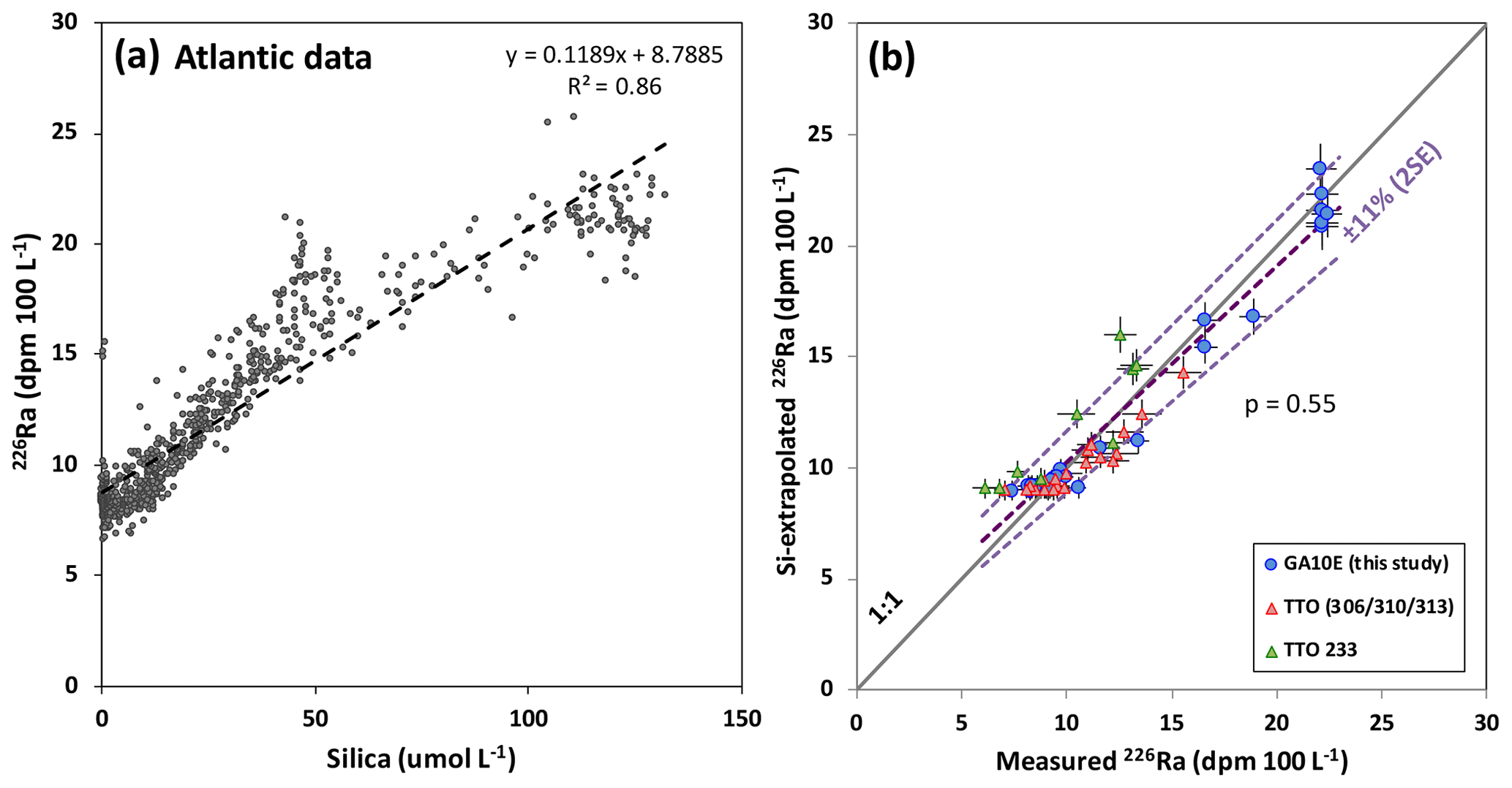
Figure A1(a) Relationship between the Atlantic seawater 226Ra activity and silica concentration (GEOTRACES GA03, GEOSECS, and TTO datasets; Ku and Lin, 1976; Key et al., 1990, 1992a, b; Charette et al., 2015). The dashed line shows a linear regression through all the data. (b) Plots of Si-extrapolated 226Ra against measured 226Ra in this study and the TTO programme. The paired t test shows a p value of 0.55 (>0.05). The solid line is 1 : 1, and the dashed purple lines show the linear regressions with the error bars of ±11 % (2 SE).
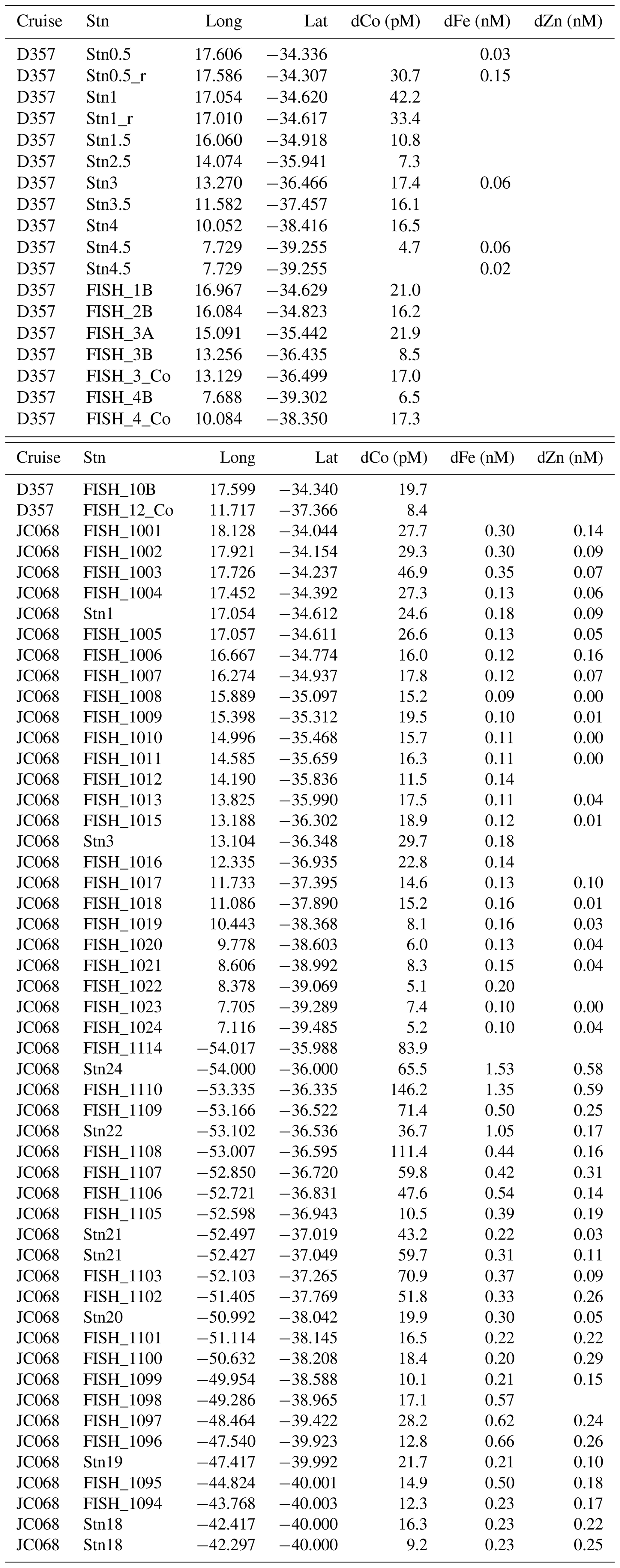

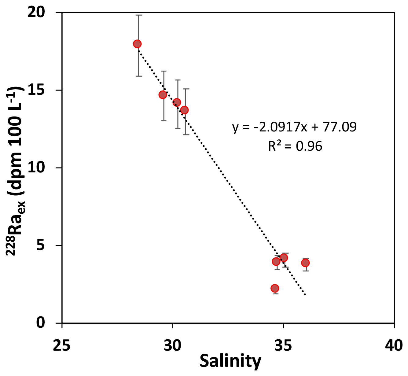
Figure C1Relationship between seawater 228Raex activity and salinity in the Argentine Basin. The dashed line shows the linear regression. The error bars of 228Raex activity are 2 SE.
D1 228Ra-derived diffusive TE fluxes
To calculate both lateral and vertical TE fluxes, the 228Ra-derived diffusion coefficients (Kz or Kx) are applied to Eq. (6) with the gradient of TE concentration ( or Δz) over either the horizontal distance x to the coasts or the vertical depth z below the mixed layer, which can be obtained from the linear regression of horizontal and vertical TE profiles in Figs. 3 and 4, respectively. In the Argentine Basin, the cross-shelf horizontal gradients of TEs (Fig. 3a, c, and e) and 228Ra-derived Kx (Fig. 5a) have been used to assess the TE fluxes cross the shelf break and the Brazil Current. In the Cape Basin, where the TE gradients (Co and Fe) from both cruises (D357 and JC068) are used for comparison (Fig. 3b and d), the differences are generally less than 20 % (except for the vertical gradient of Co at Stn3). As the vertical gradients and 228Ra-derived Kz in the Argentine Basin are likely to be biased by lateral inputs, the vertical TE fluxes are not assessed in the western transect here. The 228Ra-derived diffusive TE fluxes are summarised in Table 2 (horizontal) and Table 3 (vertical).
D2 228Ra-derived advective TE fluxes
The advective TE fluxes after the boundary of the shelf break and the Brazil Current in the Argentine Basin can be calculated using Eq. (7) with the net offshore advection velocity ( cm s−1) along the SAC in the Argentine Basin and the average concentrations of dissolved TEs in the initial advective waters around where the Brazil Current merges into the SAC (around Stn21; Fig. 3): [Co] pM; [Fe] nM; [Zn] nM (1 SD, n=4). The calculated advective TE fluxes are summarised in Table 2 for comparison. As the advective signals cannot be easily separated from the mixing in the Cape Basin, the advective TE fluxes are not assessed in the eastern transect here.
D3 -ratio-derived TE fluxes
The cross-shelf -ratio-derived TE fluxes can be calculated using Eq. (8) with the Ra ratios reported in Table D1 and the estimates of shelf 228Ra flux (F228Ra) based on the inverse models using the global seawater 228Ra database and inventory (Kwon et al., 2014; Le Gland et al., 2017). In the South Atlantic, the average shelf 228Ra flux is atoms m2 yr−1 around the Uruguayan and South African continental margins (normalised to shelf area; Charette et al., 2016). For comparison, the flux is converted to the shelf–ocean cross-sectional flux by multiplying the average continental shelf widths (Cape Basin: 80 km; Argentine Basin: 120 km) and then dividing by the water depths at the shelf break (Cape Basin: 150 m; Argentine Basin: 160 m) (Urien and Ewing, 1974; Nelson et al., 1998; Carr and Botha, 2012). The shelf length is shared between the two surfaces (the shelf horizontal plane and vertical section in Fig. 8) and cancelled out during the calculation (Table D2). The cross-shelf 228Ra flux (F228Ra) becomes atoms m2 yr−1 in the Argentine Basin and atoms m2 yr−1 in the Cape Basin. The calculated TE fluxes are summarised in Table 2.
It is important to remember that when considering the sources of 228Ra and TEs in the ocean, TEs may have their maximum source term at a different depth than 228Ra. Whereas 228Ra has a clear maximum from the continental shelf in the surface mixed layer, redox-sensitive, more particle-bound or hydrothermal-related TEs may see a maximum at deeper levels, due to particle resuspension, low oxygen saturation, or hydrothermal activity. In this sense, our model calculations provide the estimates of lateral TE inputs in the surface mixed layer with a clear source from the continental shelf. The vertical TE inputs, however, do not separate the TE inputs between internal cycling, hydrothermal, or lateral transport from the continental margin at greater depths. Nevertheless, all these inputs would only become relevant for productivity if they reach the surface mixed layer later, e.g. by vertical mixing as quantified here.
Table D1Shelf and open-ocean average dTE and 228Ra concentrations and Ra ratios*.
* Only JC068 TE data are used. All errors are ±1 SD.
Table D2Average shelf width and shelf-break water depth for shelf–ocean dTE flux normalisationa.
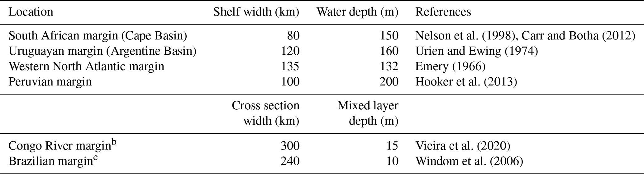
a Shelf–ocean TE or 228Ra fluxes presented in this study are normalised to the area of shelf–ocean cross section (by default, the cross section at shelf break is equal to shelf length multiplied by the shelf-break water depth). To convert the shelf TE or 228Ra flux (usually normalised by shelf area) from previous studies, the shelf fluxes are multiplied by the shelf width and length, and then divided by the area of the cross section. Shelf length should drop off from the flux conversion. a Congo River margin TE fluxes are divided by a defined cross section (the width of river plume multiplied by the mixed layer depth). b Brazilian margin Fe flux is divided by a defined cross section (the width of a defined coastline multiplied by the mixed layer depth).
All the original and supporting data are shown in the paper. The data are also available publicly at the GEOTRACES IDP2017 (https://www.bodc.ac.uk/geotraces/data/idp2017/, Schlitzer et al., 2018).
YTH, WG, and GMH designed the radium projects. YTH conducted the Ra-228 and Ra-226 analyses. EMSW conducted the Si measurements. NJW, MCL, and EPA contributed the TE data and interpretation. YTH prepared the manuscript with contributions from all co-authors.
The authors declare that they have no conflict of interest.
The authors wish to thank the officers and crew of the RRS Discovery and RRS James Cook for their assistance on the UK GEOTRACES GA10 cruises (D357 and JC068). We would like to thank Alex Thomas, Andrew Mason, and Steve Wyatt for assistance with mass spectrometry and laboratory support. We would also like to thank Willard Moore, Will Homoky, Yves Plancherel, and Christian Schlosser for feedback and discussion at different stages of the manuscript preparation. This study was funded by grants from the UK Natural Environment Research Council for the UK GEOTRACES GA10 cruises NE/H008497/1 to Walter Geibert, NE/F017316/1 to Gideon M. Henderson, NE/H004475/1 to Maeve C. Lohan and Neil J. Wyatt, and NE/H004394/1 to Eric P. Achterberg.
This research has been supported by the Natural Environment Research Council (grant nos. NE/H008497/1 to Walter Geibert, NE/F017316/1 to Gideon M. Henderson, NE/H004475/1 to Maeve C. Lohan and Neil J. Wyatt, and NE/H004394/1 to Eric P. Achterberg).
This paper was edited by Markus Kienast and reviewed by two anonymous referees.
Achterberg, E. P., Steigenberger, S., Marsay, C. M., LeMoigne, F. A. C., Painter, S. C., Baker, A. R., Connelly, D. P., Moore, C. M., Tagliabue, A., and Tanhua, T.: Iron biogeochemistry in the high latitude North Atlantic Ocean, Sci. Rep., 8, 1283, https://doi.org/10.1038/s41598-018-19472-1, 2018.
Achterberg, E. P., Steigenberger, S., Klar, J. K., Browning, T. J., Marsay, C. M., Painter, S. C., Vieira, L., Baker, A. R., Hamilton, D. S., Tanhua, T., and Moore, C. M.: Trace element biogeochemistry in the high latitude North Atlantic Ocean; seasonal variations and volcanic inputs, Global Biogeochem. Cy., e2020GB006674, https://doi.org/10.1029/2020GB006674, online first, 2020.
Beal, L. M., De Ruijter, W. P. M., Biastoch, A., Zahn, R., and the SCOR/WCRP/IAPSO Working Group 136: On the role of the Agulhas system in ocean circulation and climate, Nature, 472, 429–436, https://doi.org/10.1038/nature09983, 2011.
Blain, S., Quéguiner, B., Armand, L., Belviso, S., Bombled, B., Bopp, L., Bowie, A., Brunet, C., Brussaard, C., Carlotti, F., Christaki, U., Corbière, A., Durand, I., Ebersbach, F., Fuda, J.-L., Garcia, N., Gerringa, L., Griffiths, B., Guigue, C., Guillerm, C., Jacquet, S., Jeandel, C., Laan, P., Lefèvre, D., Monaco, C. L., Malits, A., Mosseri, J., Obernosterer, I., Park, Y.-H., Picheral, M., Pondaven, P., Remenyi, T., Sandroni, V., Sarthou, G., Savoye, N., Scouarnec, L., Souhaut, M., Thuiller, D., Timmermans, K., Trull, T., Uitz, J., van Beek, P., Veldhuis, M., Vincent, D., Viollier, E., Vong, L., and Wagener T.: Effect of natural iron fertilization on carbon sequestration in the Southern Ocean, Nature, 446, 1070–1074, https://doi.org/10.1038/nature05700, 2007.
Bown, J., Boye, M., Baker, A., Duvieilbourg, E., Lacan, F., Le Moigne, F., Planchon, F., Speich, S., and Nelson, D. M.: The biogeochemical cycle of dissolved cobalt in the Atlantic and the Southern Ocean south off the coast of South Africa, Mar. Chem., 126, 193–206, https://doi.org/10.1016/j.marchem.2011.03.008, 2011.
Broecker, W. S., Goddard, J., and Sarmiento, J. L.: Distribution of Ra-226 in Atlantic Ocean, Earth Planet. Sci. Lett., 32, 220–235, https://doi.org/10.1016/0012-821X(76)90063-7, 1976.
Browning, T. J., Bouman, H. A., Moore, C. M., Schlosser, C., Tarran, G. A., Woodward, E. M. S., and Henderson, G. M.: Nutrient regimes control phytoplankton ecophysiology in the South Atlantic, Biogeosciences, 11, 463–479, https://doi.org/10.5194/bg-11-463-2014, 2014.
Browning, T. J., Achterberg, E. P., Yong, J. C., Rapp, I., Utermann, C., and Moore, C. M.: Iron limitation of microbial phosphorus acquisition in the tropical North Atlantic, Nat. Commun., 8, 15465, https://doi.org/10.1038/ncomms15465, 2017.
Bruland, K. W. and Franks, R. P.: Mn, Ni, Cu, Zn and Cd in the Western North Atlantic, in: Trace Metals in Sea Water, edited by: Wong, C. S., Boyle, E., Bruland, K. W., Burton, J. D., and Goldberg, E. D., Springer, Boston, MA, USA, 395–414, https://doi.org/10.1007/978-1-4757-6864-0_23, 1983.
Cai, P., Huang, Y., Chen, M., Guo, L., Liu, G., and, Qiu, Y.: New production based on Ra-228-derived nutrient budgets and thorium-estimated POC export at the intercalibration station in the South China Sea, Deep-Sea Res., 49, 53–66, https://doi.org/10.1016/S0967-0637(01)00040-1, 2002.
Carr, A. S. and Botha, G. A.: Coastal Geomorphology, in: Southern African Geomorphology: Recent Trends and New Directions, edited by: Holmes, P. and Meadows, M. E., Sun Press, Bloemfontein, South Africa, 269–303, 2012.
Chance, R., Jickells, T. D., and Baker, A. R.: Atmospheric trace metal concentrations, solubility and deposition fluxes in remote marine air over the south-east Atlantic, Mar. Chem., 177, 45–56, https://doi.org/10.1016/j.marchem.2015.06.028, 2015.
Charette, M. A., Gonneea, M. E., Morris, P. J., Statham, P., Fones, G., Planquette, H., Salter, I., and Garabato, A. N.: Radium isotopes as tracers of iron sources fueling a Southern Ocean phytoplankton bloom, Deep-Sea Res., 54, 1989–1998, https://doi.org/10.1016/j.dsr2.2007.06.003, 2007.
Charette, M. A., Morris, P. J., Henderson, P. B., and Moore, W. S.: Radium isotope distributions during the US GEOTRACES North Atlantic cruises, Mar. Chem., 177, 184–195, https://doi.org/10.1016/j.marchem.2015.01.001, 2015.
Charette, M. A., Lam, P. J., Lohan, M. C., Kwon, E. Y., Hatje, V., Jeandel, C., Shiller, A. M., Cutter, G. A., Thomas, A., Boyd, P. W., Homoky, W. B., Milne, A., Thomas, H., Andersson, P. S., Porcelli, D., Tanaka, T., Geibert, W., Dehairs, F., and Garcia-Orellana, J.: Coastal ocean and shelf-sea biogeochemical cycling of trace elements and isotopes: lessons learned from GEOTRACES, Philos. T. R. Soc. A, 374, 20160076, https://doi.org/10.1098/rsta.2016.0076, 2016.
Chever, F., Bucciarelli, E., Sarthou, G., Speich, S., Arhan, M., Penven, P., and Tagliabue, A.: Physical speciation of iron in the Atlantic sector of the Southern Ocean along a transect from the subtropical domain to the Weddell Sea Gyre, J. Geophys. Res.-Oceans, 115, C10059, https://doi.org/10.1029/2009JC005880, 2010.
Clough, R., Floor, G. H., Quétel, C. R., Milne, A., Lohan, M. C., and Worsfold, P. J.: Measurement uncertainty associated with shipboard sample collection and filtration for the determination of the concentration of iron in seawater, Anal. Methods, 8, 6711–6719, https://doi.org/10.1039/C6AY01551D, 2016.
Cochran, J. K.: The oceanic chemistry of the uranium- and thorium-series nuclides, in: Uranium-Series Disequilibrium: Applications to Earth, Marine, and Environmental Sciences, edited by: Ivanovich, M. and Harmon R. S., Clarendon Press, Oxford, UK, 334–391, 1992.
Cutter, G, Andersson, P., Codispoti, L, Croot, P., Francois, R., Lohan, M. C., Obata, H., and Rutgers van der Loeff, M.: Sampling and sample-handling protocols for GEOTRACES cruises, available at: http://www.geotraces.org/libraries/documents/Intercalibration/Cookbook.pdf (last access: 10 January 2021), 2010.
Dulaiova, H., Ardelan, M. V., Henderson, P. B., and Charette, M. A.: Shelf-derived iron inputs drive biological productivity in the southern Drake Passage, Global Biogeochem. Cy., 23, GB4014, https://doi.org/10.1029/2008GB003406, 2009.
Emery, K. O.: Atlantic continental shelf and slope of the United States: U.S. Geological Survey Professional Papers, 529, 1–23, 1966.
Foster, D. A., Staubwasser, M., and Henderson, G. M.: Ra-226 and Ba concentrations in the Ross Sea measured with multicollector ICP mass spectrometry, Mar. Chem., 87, 59–71, https://doi.org/10.1016/j.marchem.2004.02.003, 2004.
Gaiero, D. M., Simonella, L., Gassó, S., Gili, S., Stein, A. F., Sosa, P., Becchio, R., Arce, J., and Marelli, H.: Ground/satellite observations and atmospheric modeling of dust storms originating in the high Puna- Altiplano deserts (South America), implications for the interpretation of paleo-climatic archives, J. Geophys. Res.-Atmos., 118, 3817–3831, https://doi.org/10.1002/jgrd.50036, 2013.
Geibert, W., Rodellas, V., Annett, A., van Beek, P., Garcia-Orellana, J., Hsieh, Y.-T., and Masque, P.: 226Ra determination via the rate of 222Rn ingrowth with the Radium Delayed Coincidence Counter (RaDeCC), Limnol. Oceanogr.-Meth., 11, 594–603, https://doi.org/10.4319/lom.2013.11.594, 2013.
Graham, R. M., De Boer, A. M., van Sebille, E., Kohfeld, K. E., and Schlosser, C.: Inferring source regions and supply mechanisms of iron in the Southern Ocean from satellite chlorophyll data, Deep Sea Res., 104, 9–25, https://doi.org/10.1016/j.dsr.2015.05.007, 2015.
Hanfland, C.: Radium-226 and Radium-228 in the Atlantic sector of the Southern Ocean, PhD thesis, Alfred Wegener Institut fur Polar und Meeresforschung, Bremerhaven, Germany, 135 pp., 2002.
Hawco, N. J., Ohnemus, D. C., Resing, J. A., Twining, B. S., and Saito, M. A.: A dissolved cobalt plume in the oxygen minimum zone of the eastern tropical South Pacific, Biogeosciences, 13, 5697–5717, https://doi.org/10.5194/bg-13-5697-2016, 2016.
Hayes, C. T., Black, E. E., Anderson, R. F., Baskaran, M., Buesseler, K. O., Charette, M. A., Cheng, H., Cochran, J. K., Edwards, R. L., Fitzgerald, P., Lam, P. J., Lu, Y., Morris, S. O., Ohnemus, D. C., Pavia, F. J., Stewart, G., and Tang, Y.: Flux of Particulate Elements in the North Atlantic Ocean Constrained by Multiple Radionuclides, Global Biogeochem. Cy., 32, 1738–1758, 2018.
Homoky, W., John, S. G., Conway, T. M., and Mills, R. A.: Distinct iron isotopic signatures and supply from marine sediment dissolution, Nat. Commun., 4, 2143, https://doi.org/10.1038/ncomms3143, 2013.
Hooker, Y., Prieto-Rios, E., and Solís-Marín, F. A.: Echinoderms of Peru, in: Echinoderm research and diversity in Latin America, edited by: Alvarado-Barrientos, J. J. and Solís-Marín, F. A., Springer, Berlin, Germany, 277–299, 2013.
Hsieh, Y.-T. and Henderson, G. M.: Precise measurement of ratios and Ra concentrations in seawater samples by multi-collector ICP mass spectrometry, J. Anal. Atom. Spect., 26, 1338–1346, https://doi.org/10.1039/C1JA10013K, 2011.
Jenkins, W. J.: Nitrate Flux into the Euphotic Zone near Bermuda, Nature, 331, 521–523, https://doi.org/10.1038/331521a0, 1988.
Kadko, D., Aguilar-Islas, A., Buck, C. S., Fitzsimmons, J. N., Landing, W. M., Shiller, A., Till, C. P., Bruland, K. W., Boyle, E. A., and Anderson, R. F.: Sources, fluxes and residence times of trace elements measured during the U.S. GEOTRACES East Pacific Zonal Transect, Mar. Chem., 222, 103781, https://doi.org/10.1016/j.marchem.2020.103781, 2020.
Kaufman, A., Trier, R., Broecker, W. S., and Feely, H. W.: Distribution of 228Ra in the world ocean, J. Geophys. Res., 78, 8827–8848, https://doi.org/10.1029/JC078i036p08827, 1973.
Key, R. M., Rotter, R. J., McDonald, G. J., and Slater, R. D.: Western Boundary Exchange Experiment Final Data Report for large volume samples 228Ra, 226Ra, 9Be, and 10Be Results, Technical Report 90-1, Ocean Tracer Laboratory, Department of Geology and Geophysics, Princeton University, Princeton, USA, 298 pp., 1990.
Key, R. M., Moore, W. S., and Sarmiento, J. L.: Transient Tracers in the Ocean North Atlantic Study Final Data Report for 228Ra and 226Ra, Technical Report 92-2, Ocean Tracer Laboratory, Department of Geology and Geophysics, Princeton University, Princeton, USA, 193 pp., 1992a.
Key, R. M., Moore, W. S., and Sarmiento, J. L.: Transient Tracers in the Ocean Tropical Atlantic Study Final Data Report for 228Ra and 226Ra, Technical Report 92-3, Ocean Tracer Laboratory, Department of Geology and Geophysics, Princeton University, Princeton, USA, 298 pp., 1992b.
Kipp, L. E., Charette, M. A., Moore, W. S., Henderson, P. B., and Rigor, I. G.: Increased fluxes of shelf-derived materials to the central Arctic Ocean, Sci. Adv., 4, eaao1302, https://doi.org/10.1126/sciadv.aao1302, 2018a.
Kipp, L. E., Sanial, V., Henderson, P. B., van Beek, P., Reyss, J.-L., Hammond, D. E., Moore, W. S., and Charette, M. A.: Radium isotopes as tracers of hydrothermal inputs and neutrally buoyant plume dynamics in the deep ocean, Mar. Chem., 201, 51–65, https://doi.org/10.1016/j.marchem.2017.06.011, 2018b.
Knauss, K. G., Ku, T. L., and Moore, W. S.: Radium and Thorium Isotopes in Surface Waters of East Pacific and Coastal Southern-California, Earth Planet. Sci. Lett., 39, 235–249, https://doi.org/10.1016/0012-821X(78)90199-1, 1978.
Ku, T. L. and Lin, M. C.: Ra-226 Distribution in Antarctic Ocean, Earth Planet. Sci. Lett., 32, 236–248, https://doi.org/10.1016/0012-821X(76)90064-9, 1976.
Ku, T. L. and Luo, S.: Ocean circulation/mixing studies with decay-series isotopes, in: U-Th Series Nuclides in Aquatic Systems, edited by: Krishnaswami, S. and Cochran, J. K., Elsevier, Oxford, UK, 307–344, 2008.
Ku, T. L., Luo, S. D., Kusakabe, M., and Bishop, J. K. B.: Ra-228-Derived Nutrient Budgets in the Upper Equatorial Pacific and the Role of New Silicate in Limiting Productivity, Deep-Sea Res., 42, 479–497, https://doi.org/10.1016/0967-0645(95)00020-Q, 1995.
Kunze, E. and Sanford, T. B.: Abyssal mixing: Where it is not, J. Phys. Oceanogr., 26, 2286–2296, https://doi.org/10.1175/1520-0485(1996)026<2286:AMWIIN>2.0.CO;2, 1996.
Kwon, E. Y., Kim, G., Primeau, F., Moore, W. S., Cho, H.-M., DeVries, T., Sarmiento, J. L., Charette, M. A., and Cho, Y.-K.: Global estimate of submarine groundwater discharge based on an observationally constrained radium isotope model, Geophys. Res. Lett., 41, 8438–8444, https://doi.org/10.1002/2014GL061574, 2014.
Lamontagne, S. and Webster, I. T.: Theoretical assessment of the effect of vertical dispersivity on coastal seawater radium distribution, Front. Mar. Sci., 6, 357, https://doi.org/10.3389/fmars.2019.00357, 2019.
Ledwell, J. R., Watson, A. J., and Law, C. S.: Evidence for slow mixing across the pycnocline from an open-ocean tracer-release experiment, Nature, 364, 701–703, https://doi.org/10.1038/364701a0, 1993.
Le Gland, G., Mémery, L., Aumont, O., and Resplandy, L.: Improving the inverse modeling of a trace isotope: how precisely can radium-228 fluxes toward the ocean and submarine groundwater discharge be estimated?, Biogeosciences, 14, 3171–3189, https://doi.org/10.5194/bg-14-3171-2017, 2017.
Li, Y. H., Peng, T. H., Broecker, W. S., and Ostlund, H. G.: The Average Vertical Mixing Coefficient for the Oceanic Thermocline, Tellus B, 36, 212–217, https://doi.org/10.3402/tellusb.v36i3.14905, 1984.
Liang, X., Spall, M., and Wunsch, C.: Global ocean vertical velocity from a dynamically consistent ocean state estimate, J. Geophys. Res.-Oceans, 122, 8208–8224, https://doi.org/10.1002/2017JC012985, 2017.
Lohan, M. C. and Tagliabue, A.: Oceanic Micronutrients: trace metals that are essential for marine life, Elements, 14, 385–390, https://doi.org/10.2138/gselements.14.6.385, 2018.
Longhurst, A. R.: Ecological Geography of the Sea, Academic Press, Burlington, VT, USA, https://doi.org/10.1016/B978-0-12-455521-1.X5000-1, 2007.
Martin, A. P., Lucas, M. I., Painter, S. C., Pidcock, R., Prandke, H., Prandke, H., and Stinchcombe, M. C.: The supply of nutrients due to vertical turbulent mixing: a study at the Porcupine Abyssal Plain study site (49∘50′ N 16∘30′ W) in the Northeast Atlantic, Deep-Sea Res., 57, 1293–1302, https://doi.org/10.1016/j.dsr2.2010.01.006, 2010.
Menzel Barraqueta, J.-L., Klar, J. K., Gledhill, M., Schlosser, C., Shelley, R., Planquette, H. F., Wenzel, B., Sarthou, G., and Achterberg, E. P.: Atmospheric deposition fluxes over the Atlantic Ocean: a GEOTRACES case study, Biogeosciences, 16, 1525–1542, https://doi.org/10.5194/bg-16-1525-2019, 2019.
Moore, C. M., Mills, M. M., Arrigo, K. R., Berman-Frank, I., Bopp, L., Boyd, P. W., Galbraith, E. D., Geider, R. J., Guieu, C., Jaccard, S. L., Jickells, T. D., La Roche, J., Lenton, T. M., Mahowald, N. M., Earanon, E., Marinov, I., Moore, J. K., Nakatsuka, T., Oschlies, A., Saito, M. A., Thingstad, T. F., Tsuda, A., and Ulloa, O.: Processes and patterns of oceanic nutrient limitation, Nat. Geosci., 6, 701–710, https://doi.org/10.1038/ngeo1765, 2013.
Moore, J. K., Doney, S. C., and Lindsay, K.: Upper ocean ecosystem dynamics and iron cycling in a global three-dimensional model, Global Biogeochem. Cy., 18, GB4028, https://doi.org/10.1029/2004GB002220, 2004.
Moore, W. S.: Determining coastal mixing rates using radium isotopes, Cont. Shelf Res., 20, 1993–2007, https://doi.org/10.1016/S0278-4343(00)00054-6, 2000.
Moore, W. S.: Inappropriate attempts to use distributions of 228Ra and 226Ra in coastal waters to model mixing and advection rates, Cont. Shelf Res., 105, 95–100, https://doi.org/10.1016/j.csr.2015.05.014, 2015.
Moore, W. S. and Arnold, R.: Measurement of Ra-223 and Ra-224 in coastal waters using a delayed coincidence counter, J. Geophys. Res.-Oceans, 101, 1321–1329, https://doi.org/10.1029/95JC03139, 1996.
Moore, W. S. and Dymond, J.: Fluxes of Ra-226 and Barium in the Pacific-Ocean – the Importance of Boundary Processes, Earth Planet. Sci. Lett., 107, 55–68, https://doi.org/10.1016/0012-821X(91)90043-H, 1991.
Moore, W. S., Key, R. M., and Sarmiento, J. L.: Techniques for Precise Mapping of Ra-226 and Ra-228 in the Ocean, J. Geophys. Res.-Oceans, 90, 6983–6994, https://doi.org/10.1029/JC090iC04p06983, 1985.
Moore, W. S., Sarmiento, J. L., and Key, R. M.: Submarine groundwater discharge revealed by 228Ra distribution in the upper Atlantic Ocean, Nat. Geosci., 1, 309–311, https://doi.org/10.1038/ngeo183, 2008.
Morel, F. M. M. and Price, N. M.: The biogeochemical cycles of trace metals in the oceans, Science, 300, 944–947, https://doi.org/10.1126/science.1083545, 2003.
Nelson, G., Boyd, A. J., Agenbag, J. J., and Duncombe Rae, C. M.: An upwelling filament north-west of Cape Town, South Africa, S. Afr. J. Marine Sci., 19, 75–88, https://doi.org/10.2989/025776198784126953, 1998.
Noble, A. E., Lamborg, C. H, Ohnemus, D. C., Lam, P. J., Goepfert, T. J., Measures, C. I., Frame, C. H., Casciotti, K. L., DiTullio, G. R., Jennings, J., and Saito, M. A.: Basin-scale inputs of cobalt, iron, and manganese from the Benguela-Angola front to the South Atlantic Ocean, Limnol. Oceanogr., 57, 989–1010, https://doi.org/10.4319/lo.2012.57.4.0989, 2012.
Noble, A. E., Ohnemus, D. C., Hawco, N. J., Lam, P. J., and Saito, M. A.: Coastal sources, sinks and strong organic complexation of dissolved cobalt within the US North Atlantic GEOTRACES transect GA03, Biogeosciences, 14, 2715–2739, https://doi.org/10.5194/bg-14-2715-2017, 2017.
Nozaki, Y. and Yamamoto, Y.: Radium 228 based nitrate fluxes in the eastern Indian Ocean and the South China Sea and a silicon-induced “alkalinity pump” hypothesis, Global Biogeochem. Cy., 15, 555–567, https://doi.org/10.1029/2000GB001309, 2001.
Oschlies, A.: Nutrient supply to the surface waters of the North Atlantic: A model study, J. Geophys. Res.-Oceans, 107, 3046, https://doi.org/10.1029/2000JC000275, 2002.
Owens, S. A., Pike, S., and Buesseler, K. O.: Thorium-234 as a tracer of particle dynamics and upper ocean export in the Atlantic Ocean, Deep Sea Res., 116, 42–59, https://doi.org/10.1016/j.dsr2.2014.11.010, 2015.
Painter, S. C., Henson, S. A., Forryan, A., Steigenberger, S., Klar, J., Stinchcombe, M. C., Rogan, N., Baker, A. R., Achterberg, E. P., and Moore, C. M.: An assessment of the vertical diffusive flux of iron and other nutrients to the surface waters of the subpolar North Atlantic Ocean, Biogeosciences, 11, 2113–2130, https://doi.org/10.5194/bg-11-2113-2014, 2014.
Paul, M., Van De Flierdt, T., Rehkämper, M., Khondoker, R., Weiss, D., Lohan, M. C., and Homoky, W. B.: Tracing the Agulhas leakage with lead isotopes, Geophys. Res. Lett., 42, 8515–8521, https://doi.org/10.1002/2015GL065625, 2015.
Price, N. M. and Morel, F. M. M.: Cadmium and cobalt substitution for zinc in a marine diatom, Nature, 344, 658–660, 1990.
Reid, D. F., Key, R. M., and Schink, D. R.: Radium, Thorium and Actinium extraction from seawater using an improved manganese-oxide-coated fiber, Earth Planet. Sci. Lett., 43, 223–226, https://doi.org/10.1016/0012-821X(79)90205-X, 1979.
Rigby, S. J., Williams, R. G., Achterberg, E. P., and Tagliabue, A.: Resource availability and entrainment are driven by offsets between nutriclines and winter mixed-layer depth, Global Biogeochem. Cy., 34, e2019GB006497, https://doi.org/10.1029/2019GB006497, 2020.
Rijkenberg, M. J. A., Middag, R., Laan, P., Gerringa, L. J. A., van Aken, H. M., Schoemann, V., de Jong, J. T. M., and de Baar, H. J. W.: The distribution of dissolved iron in the west Atlantic Ocean, PLoS One, 9, e101323, https://doi.org/10.1371/journal.pone.0101323, 2014.
Rodellas, V., Garcia-Orellana, J., Masqué, P., Feldman, M., and Weinstein, Y.: Submarine groundwater discharge as a major source of nutrients to the Mediterranean Sea, P. Natl. Acad. Sci., 12, 3926–3930, https://doi.org/10.1073/pnas.1419049112, 2015.
Rutgers van der Loeff, M. M., Key, R. M., Scholten, J., Bauch, D., and Michel, A.: 228Ra as a tracer for shelf water in the arctic ocean, Deep. Sea Res., 42, 1533–1553, https://doi.org/10.1016/0967-0645(95)00053-4, 1995.
Saito, M. A., Noble, A. E., Tagliabue, A., Goepfert, T. J., Lamborg, C. H., and Jenkins, W. J.: Slow-spreading submarine ridges in the South Atlantic as a significant oceanic iron source, Nat. Geosci., 6, 775–779, https://doi.org/10.1038/ngeo1893, 2013.
Sanial, V., Kipp, L. E., Henderson, P. B., van Beek, P., Reyss, J.-L., Hammond, D. E., Hawco, N., Saito, M. A., Resing, J. A., Sedwick, P. N., Moore, W. S., and Charette, M. A.: Radium-228 as a tracer of dissolved trace element inputs from the Peruvian continental margin, Mar. Chem., 201, 20–34, https://doi.org/10.1016/j.marchem.2017.05.008, 2018.
Sarmiento, J. L., Feely, H. W., Moore, W. S., Bainbridge, A. E., and Broecker, W. S.: Relationship between Vertical Eddy Diffusion and Buoyancy Gradient in Deep-Sea, Earth Planet. Sci. Lett., 32, 357–370, https://doi.org/10.1016/0012-821X(76)90076-5, 1976.
Sarmiento, J. L., Thiele, G., Key, R. M., and Moore, W. S.: Oxygen and Nitrate New Production and Remineralization in the North-Atlantic Subtropical Gyre, J. Geophys. Res.-Oceans, 95, 18303–18315, https://doi.org/10.1029/JC095iC10p18303, 1990.
Schlitzer, R.: Mass and Heat Transport in the South Atlantic Derived from Historical Hydrographie Data, edited by: Wefer, G., Berger, W. H., Siedler, G., and Webb, D. J. , in: The South Atlantic, Springer, Berlin and Heidelberg, Germany, 305–323, https://doi.org/10.1007/978-3-642-80353-6_17, 1996.
Schlitzer, R.: Quantifying He fluxes from the mantle using multi-tracer data assimilation, Philos. T. R. Soc. A, 374, 20150288, https://doi.org/10.1098/rsta.2015.0288, 2016.
Schlitzer, R., Anderson, R. F., Dodas, E. M., Lohan, M., Geibert, W., Tagliabue, A., Bowie, A., Jeandel, C., Maldonado, M. T., Landing, W. M., Cockwell, D., Abadie, C., Abouchami, W., Achterberg, E. P., Agather, A., Aguliar-Islas, A., van Aken, H. M., Andersen, M., Archer, C., Auro, M., de Baar, H. J., Baars, O., Baker, A. R., Bakker, K., Basak, C., Baskaran, M., Bates, N. R., Bauch, D., van Beek, P., Behrens, M. K., Black, E., Bluhm, K., Bopp, L., Bouman, H., Bowman, K., Bown, J., Boyd, P., Boye, M., Boyle, E. A., Branellec, P., Bridgestock, L., Brissebrat, G., Browning, T., Bruland, K. W., Brumsack, H.-J., Brzezinski, M., Buck, C. S., Buck, K. N., Buesseler, K., Bull, A., Butler, E., Cai, P., Cámara Mor, P., Cardinal, D., Carlson, C., Carrasco, G., Casacuberta, N., Casciotti, K. L., Castrillejo, M., Chamizo, E., Chance, R., Charette, M. A., Chaves, J. E., Cheng, H., Chever, F., Christl, M., Church, T. M., Closset, I., Colman, A., Conway, T. M., Cossa, D., Croot, P., Cullen, J. T., Cutter, G. A., Daniels, C., Dehairs, F., Deng, F., Dieu, H. T., Duggan, B., Dulaquais, G., Dumousseaud, C., Echegoyen-Sanz, Y., Edwards, R. L., Ellwood, M., Fahrbach, E., Fitzsimmons, J. N., Flegal, A. R., Fleisher, M. Q., van de Flierdt, T., Frank, M., Friedrich, J., Fripiat, F., Fröllje, H., Galer, S. J. G., Gamo, T., Ganeshram, R. S., Garcia-Orellana, J., Garcia-Solsona, E., Gault-Ringold, M., George, E., Gerringa, L. J. A., Gilbert, M., Godoy, J. M., Goldstein, S. L., Gonzalez, S. R., Grissom, K., Hammerschmidt, C., Hartman, A., Hassler, C. S., Hathorne, E. C., Hatta, M., Hawco, N., Hayes, C. T., Heimbürger, L.-E., Helgoe, J., Heller, M., Henderson, G. M., Henderson, P. B., van Heuven, S., Ho, P., Horner, T. J., Hsieh, Y.-T., Huang, K.-F., Humphreys, M. P., Isshiki, K., Jacquot, J. E., Janssen, D. J., Jenkins, W. J., John, S., Jones, E. M., Jones, J. L., Kadko, D. C., Kayser, R., Kenna, T. C., Khondoker, R., Kim, T., Kipp, L., Klar, J. K., Klunder, M., Kretschmer, S., Kumamoto, Y., Laan, P., Labatut, M., Lacan, F., Lam, P. J., Lambelet, M., Lamborg, C. H., Le Moigne, F. A. C., Le Roy, E., Lechtenfeld, O. J., Lee, J.-M., Lherminier, P., Little, S., López-Lora, M., Lu, Y., Masque, P., Mawji, E., Mcclain, C. R., Measures, C., Mehic, S., Barraqueta, J.-L. M., van der Merwe, P., Middag, R., Mieruch, S., Milne, A., Minami, T., Moffett, J. W., Moncoiffe, G., Moore, W. S., Morris, P. J., Morton, P. L., Nakaguchi, Y., Nakayama, N., Niedermiller, J., Nishioka, J., Nishiuchi, A., Noble, A., Obata, H., Ober, S., Ohnemus, D. C., van Ooijen, J., O'Sullivan, J., Owens, S., Pahnke, K., Paul, M., Pavia, F., Pena, L. D., Peters, B., Planchon, F., Planquette, H., Pradoux, C., Puigcorbé, V., Quay, P., Queroue, F., Radic, A., Rauschenberg, S., Rehkämper, M., Rember, R., Remenyi, T., Resing, J. A., Rickli, J., Rigaud, S., Rijkenberg, M. J. A., Rintoul, S., Robinson, L. R., Roca-Martí, M., Rodellas, V., Roeske, T., Rolison, J. M., Rosenberg, M., Roshan, S., Rutgers van der Loeff, M. M., Ryabenko, E., Saito, M. A., Salt, L. A., Sanial, V., Sarthou, G., Schallenberg, C., Schauer, U., Scher, H., Schlosser, C., Schnetger, B., Scott, P., Sedwick, P. N., Semiletov, I., Shelley, R., Sherrell, R. M., Shiller, A. M., Sigman, D. M., Singh, S. K., Slagter, H. A., Slater, E., Smethie, W. M., Snaith, H., Sohrin, Y., Sohst, B., Sonke, J. E., Speich, S., Steinfeldt, R., Stewart, G., Stichel, T., Stirling, C. H., Stutsman, J., Swarr, G. J., Swift, J. H., Thomas, A., Thorne, K., Till, C. P., Till, R., Townsend, A. T., Townsend, E., Tuerena, R., Twining, B. S., Vance, D., Velazquez, S., Venchiarutti, C., Villa-Alfageme, M., Vivancos, S. M., Voelker, A. H. L., Wake, B., Warner, M. J., Watson, R., van Weerlee, E., Weigand, M. A., Weinstein, Y., Weiss, D., Wisotzki, A., Woodward, E. M. S., Wu, J., Wu, Y., Wuttig, K., Wyatt, N., Xiang, Y., Xie, R. C., Xue, Z., Yoshikawa, H., Zhang, J., Zhang, P., Zhao, Y., Zheng, L., Zheng, X.-T., Zieringer, M., Zimmer, L. A., Ziveri, P., Zunino, P., and Zurbrick, C.: The GEOTRACES Intermediate Data Product 2017, Chem. Geol., 493, 210–223, https://doi.org/10.1016/j.chemgeo.2018.05.040, 2018 (data available at: https://www.bodc.ac.uk/geotraces/data/idp2017/, last access: 1 September 2020).
Sunda, W. G. and Huntsman, S. A.: Cobalt and zinc interreplacement in marine phytoplankton: Biological and geochemical implications, Limnol. Oceanogr., 40, 1404–1417, https://doi.org/10.4319/lo.1995.40.8.1404, 1995.
Sunda, W. G. and Huntsman, S. A.: Interrelated influence of iron, light and cell size on marine phytoplankton growth, Nature, 390, 389–392, https://doi.org/10.1038/37093, 1997.
Sunda, W. G. and Huntsman, S. A.: Effect of Zn, Mn and Fe on Cd accumulation in phytoplankton: Implications for oceanic Cd cycling, Limnol. Oceanogr., 45, 1501–1516, https://doi.org/10.4319/lo.2000.45.7.1501, 2000.
Tagliabue, A., Sallee, J. B., Bowie, A. R., Levy, M., Swart, S., and Boyd, P. W.: Surface-water iron supplies in the Southern Ocean sustained by deep winter mixing, Nat. Geosci., 7, 314–320, https://doi.org/10.1038/Ngeo2101, 2014.
Thomalla, S., Turnewitsch, R., Lucas, M., and Poulton, A.: Particulate organic carbon export from the North and South Atlantic gyres: the 234Th/238U disequilibrium approach, Deep Sea Res., 53, 1629–1648, https://doi.org/10.1016/j.dsr2.2006.05.018, 2006.
Urien, C. M. and Ewing, M.: Recent Sediments and Environment of Southern Brazil, Uruguay, Buenos Aires, and Rio Negro Continental Shelf, in: The Geology of Continental Margins, edited by: Burk, C. A. and Drake, C. L., Springer, Berlin and Heidelberg, Germany, 157–177, https://doi.org/10.1007/978-3-662-01141-6_12, 1974.
van Beek, P., Bourquin, M., Reyss, J.-L., Souhaut, M., Charette, M. A., and Jeande, C.: Radium isotopes to investigate the water mass pathways on the Kerguelen Plateau (Southern Ocean), Deep-Sea Res., 55, 622–637, https://doi.org/10.1016/j.dsr2.2007.12.025, 2008.
Vieira, L. H., Krisch, S., Hopwood, M. J., Beck, A. J., Scholten, J., Liebetrau, V., and Achterberg, E. P.: Unprecedented Fe delivery from the Congo River margin to the South Atlantic Gyre, Nat. Commun., 11, 556, https://doi.org/10.1038/s41467-019-14255-2, 2020.
Windom, H. L., Moore, W. S., Niencheski, L. F. H., and Jahnke, R. A.: Submarine groundwater discharge: a large, previously unrecognized source of dissolved iron to the South Atlantic Ocean, Mar. Chem., 102, 252–266, https://doi.org/10.1016/j.marchem.2006.06.016, 2006.
Wyatt, N. J., Milne, A., Woodward, E. M. S., Rees, A. P., Browning, T. J., Bouman, H. A., Worsfold, P. J., and Lohan, M. C.: Biogeochemical cycling of dissolved zinc along the GEOTRACES South Atlantic transect GA10 at 40∘S, Global Biogeochem. Cy., 28, 44–56, https://doi.org/10.1002/2013GB004637, 2014.
Wyatt, N. J., Milne, A., Achterberg, E. P., Browning, T. J., Bouman, H. A., Woodward, E. M. S., and Lohan, M. C.: Seasonal cycling of zinc and cobalt in the Southeast Atlantic along the GEOTRACES GA10 section, Biogeosciences Discuss. [preprint], https://doi.org/10.5194/bg-2020-42, in review, 2020.
Yamada, M. and Nozaki, Y.: Radium Isotopes in Coastal and Open Ocean Surface Waters of the Western North Pacific, Mar. Chem., 19, 379–389, https://doi.org/10.1016/0304-4203(86)90057-5, 1986.
- Abstract
- Introduction
- Study sites and methods
- Results
- Discussion
- Conclusions
- Appendix A: Seawater 226Ra and silica concentrations
- Appendix B: TE data
- Appendix C: Relationship between seawater 228Raex and salinity in the Argentine Basin
- Appendix D: TE flux calculations
- Data availability
- Author contributions
- Competing interests
- Acknowledgements
- Financial support
- Review statement
- References