Effects of spatial variability on the exposure of fish to hypoxia: a modeling analysis for the Gulf of Mexico

The hypoxic zone in the northern Gulf of Mexico varies spatially (area, location) and temporally (onset, duration) on multiple scales. Exposure of fish to hypoxic dissolved oxygen (DO) concentrations (< 2 mg L⁻¹) is often lethal and avoided, while exposure to 2 to 4 mg L⁻¹ occurs readily and often causes the sublethal effects of decreased growth and fecundity for individuals of many species. We simulated the movement of individual fish within a high-resolution 3-D coupled hydrodynamic water quality model (FVCOM-WASP) configured for the northern Gulf of Mexico to examine how spatial variability in DO concentrations would affect fish exposure to hypoxic and sublethal DO concentrations. Eight static snapshots (spatial maps) of DO were selected from a 10 d FVCOM-WASP simulation that showed a range of spatial variation (degree of clumpiness) in sublethal DO for when total sublethal area was moderate (four maps) and for when total sublethal area was high (four maps). An additional case of allowing DO to vary in time (dynamic DO) was also included. All simulations were for 10 d and were performed for 2-D (bottom layer only) and 3-D (allows for vertical movement of fish) sets of maps. Fish movement was simulated every 15 min with each individual switching among three algorithms: tactical avoidance when exposure to hypoxic DO was imminent, strategic avoidance when exposure had occurred in the recent past, and default (independent of DO) when avoidance was not invoked. Cumulative exposure of individuals to hypoxia was higher under the high sublethal area snapshots compared to the moderate sublethal area snapshots but spatial variability in sublethal concentrations had little effect on hypoxia exposure. In contrast, relatively high exposures to sublethal DO concentrations occurred in all simulations. Spatial variability in sublethal DO had opposite effects on sublethal exposure between moderate and high sublethal area maps: the percentage of fish exposed to 2–3 mg L⁻¹ decreased with increasing variability for high sublethal area but increased for moderate sublethal area. There was also a wide range of exposures among individuals within each simulation. These results suggest that averaging DO concentrations over spatial cells and time steps can result in underestimation of sublethal effects. Our methods and results can inform how movement is simulated in larger models that are critical for assessing how management actions to reduce nutrient loadings will affect fish populations.

1 Introduction

Hypoxia is expanding at locations with historical hypoxia and is appearing in new locations in the global ocean and associated coastal waters (Breitburg et al., 2018). The hypoxic zone in the northern Gulf of Mexico (GOM) is one of the world's largest areas (up to ∼ 23 000 km²) of seasonal coastal hypoxia (Rabalais et al., 2007; Rabalais and Turner, 2019). Hypoxia is often defined as a dissolved oxygen (DO) concentration less than 2 mg L⁻¹ (Rabalais et al., 2001). In the GOM, hypoxia generally occurs between April and October (Turner and Rabalais, 1991). The formation of hypoxia is influenced by the high river discharges in the spring from the Mississippi and Atchafalaya rivers that bring nutrients and freshwater to the shelf that then trigger increased primary productivity and water column stratification. The layer of fresh river water, weak tides, and weak winds during the spring and summer all contribute to strong stratification (Rabalais et al., 2001, 2002). Organic matter resulting from nutrient-enhanced surface primary production sinks to the bottom layer where it is respired. Because of the strong stratification during summertime, oxygen supply is generally lower than respiration, thus creating conditions favorable for hypoxia development (Justic et al., 1996; Rabalais et al., 2002). Hypoxia is broken up in the fall by increased winds associated with cold fronts and cooling of surface waters. Annual summertime (late July) surveys since 1985 have documented a highly variable hypoxic area whose extent during 1985 to 2011 varied from 700 to 23 200 km² (Table S2 in Obenour et al., 2013). The areal extent of hypoxia is expected to increase under future climate change scenarios (Justic et al., 2003, 2016; Sperna Weiland et al., 2012; Lehrter et al., 2017; Rabalais and Turner, 2019). The interannual variation in hypoxic area in the GOM has been extensively analyzed using regression and simplified semi-empirical (e.g., box model) methods (Obenour et al., 2015; Scavia et al., 2017; Del Giudice et al., 2019), as well as with more complex three-dimensional coupled hydrodynamic–biogeochemical models (e.g., Fennel et al., 2013; Justić and Wang, 2014).

In addition to interannual variation, the hypoxic zone within the GOM varies spatially during the summer depending on the interaction of various physical and biological factors, local bathymetry, wind forcing, hydrodynamics, solar radiation, river freshwater and nutrient inputs, phytoplankton productivity, and zooplankton grazing (Bianchi et al., 2010). The hypoxic zone typically includes a core area that is hypoxic over most summers with outer regions where DO concentrations are typically more variable in time and space (Rabalais et al., 2007; DiMarco et al., 2010). Continuous DO measurements at fixed locations often show rapid changes (on the order of ± 1–3 mg L⁻¹ h⁻¹) in bottom DO concentrations (Babin and Rabalais, 2009; Bianchi et al., 2010; Rabalais et al., 2010; Babin, 2012). Such temporal variations have also been documented for other coastal systems (e.g., Sanford et al., 1990; Booth et al., 2014; Kraus et al., 2015). These temporal variations are caused by the combined effects of local DO dynamics and the transport of DO via the movement of water and therefore imply some degree of spatial variation. Spatial analysis of DO measured synoptically at multiple locations in the GOM shows various degrees of patchiness in hypoxia on kilometer scales (Zhang et al., 2009), and such spatial variation is common in other estuarine systems (e.g., Muller et al., 2016). Hypoxia in the GOM also varies in the vertical dimension. For example, the thickness of the hypoxic zone varied from less than a meter to 20 m over the historical record (Fig. S2 in Obenour et al., 2013). Rose et al. (2018b) summarized continuous measurements of DO obtained using a towed vehicle (Scanfish) that undulated between 2 m below the surface and 2 m above the bottom (Roman et al., 2012; Zhang et al., 2014), and documented that bottom DO can frequently change by about 0.5 mg L⁻¹ min⁻¹ on the scale of tens of meters. It seems that the more we look, the more we find that low DO varies on increasingly finer temporal and spatial scales. Understanding these finer scales is relevant for quantifying the exposure of mobile organisms such as fish.

Individual fish are affected both directly and indirectly by hypoxia. Direct effects of hypoxia on fish include mortality, and the sublethal effects of reduced fecundity and growth (Shimps et al., 2005; Stierhoff et al., 2006; Rose et al., 2009; Thomas and Rahman, 2012; Limburg and Casini, 2018, 2019). Fish and other organisms change their movement behavior to avoid lethal levels of DO (Eby and Crowder, 2002; Bell and Eggleston, 2005; Pollock et al., 2007; Craig, 2012). However, while many species avoid hypoxia (< 2 mg L⁻¹), they are still exposed to low DO concentrations (2 to 4.5 mg L⁻¹) that cause sublethal effects (Vaquer-Sunyer and Duarte, 2009; Hrycik et al., 2017). Indirect effects of hypoxia on fish include changes in mortality, growth, and fecundity that result from avoidance of low DO, causing fish to experience less suitable habitat in their new locations, as well as by direct effects of low DO on their prey and predators. Hypoxia avoidance can result in fish being forced out of preferred habitat to one where there are fewer suitable prey and less shelter from predators (Eby and Crowder, 2002). Hypoxia can also affect the size, growth, energy demands, and behavior of predators (Pollock et al., 2007; Breitburg et al., 2009) and the productivity, distribution, and composition of their zooplankton and benthic prey (Baustian et al., 2009; Levin et al., 2009; Roman et al., 2019). While effects on individuals have been well documented in the laboratory under known and fixed exposures, major challenges remain to estimate exposure of fish to dynamically changing DO in two and three dimensions (Rose et al., 2009; LaBone et al., 2019), and to translate these time-varying exposures to growth, mortality, and reproduction effects (Neilan and Rose, 2014).

The fine-scale temporal and spatial dynamics of DO have been simulated in the GOM using high-resolution, three-dimensional (3-D) coupled hydrodynamic–biogeochemical models (Fennel et al., 2016; Rose et al., 2017). These include the FVCOM-WASP (Finite Volume Coastal Ocean Model - Water Quality Analysis Simulation Program) model (Justić and Wang, 2014) and an implementation of the ROMS (Regional Ocean Modeling System) model coupled with a water quality and NPZ model (Fennel et al., 2013). FVCOM is an open-source, unstructured grid ocean circulation model (Chen et al., 2011). WASP is a water quality model with a number of modules, including one for eutrophication (Wool et al., 2006). We have previously used the FVCOM-WASP model and added the capability to simulate the fine-scale movement of individual fish (Justić and Wang, 2014; Rose et al., 2014). The same model setup used here was previously used to compare the effects of different movement algorithms (LaBone et al., 2017) and 2-D versus 3-D avoidance movement on fish exposure to hypoxia (LaBone et al., 2019).

In this paper, we build upon the analysis of LaBone et al. (2017, 2019) and quantify fish exposure to hypoxia and sublethal DO concentrations under different levels of spatial variability in DO on static maps. For comparison, we also include the dynamic DO map from which we extracted the static maps as snapshots. Spatial variability in DO on the static maps was summarized statistically to ensure that contrasting levels of spatial variability were selected for the analysis. FVCOM-WASP was used to generate the dynamic DO fields within which the individual fish moved and experienced static or dynamic (hourly changing) DO concentrations. Movement of individual fish was modeled every 15 min for 10 d on the static and dynamic maps of DO within the same grid as used by FVCOM-WASP. Effects of spatial variability in DO concentrations on exposure were compared for fish with poor versus good avoidance capabilities and with and without an option for vertical avoidance. The results for the 2-D (bottom layer) and 3-D (vertical avoidance allowed) analyses were similar, so here we focus on the 2-D results; the 3-D results are summarized in the Supplement. Our overarching hypothesis was that more spatially variable DO conditions should result in higher hypoxia and sublethal exposures. However, our results showed that the relationship between spatial variability and exposure is complex; the effects of spatial variability on sublethal exposures are highly dependent on the areal extent of sublethal DO levels.

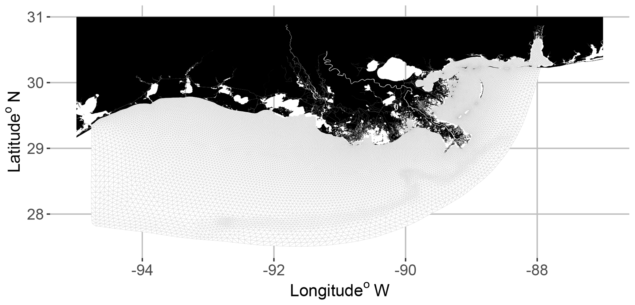
Figure 1 Planar view of the FVCOM-WASP model grid. There were also 30 vertical sigma layers.

Table 1 Areas (hypoxic, sublethal, and normoxic; km² and percent of grid) and AUC (area under the curve) values for eight snapshots selected from the hourly DO maps generated by FVCOM-WASP simulation of 10 d (20–30 August 2002). Sublethal DO was defined as 2–4 mg L⁻¹. Based on the sublethal area and AUC values, each snapshot was labeled by category of total sublethal area (S. area; high or moderate) and by category of AUC (minimum, mean, or maximum).

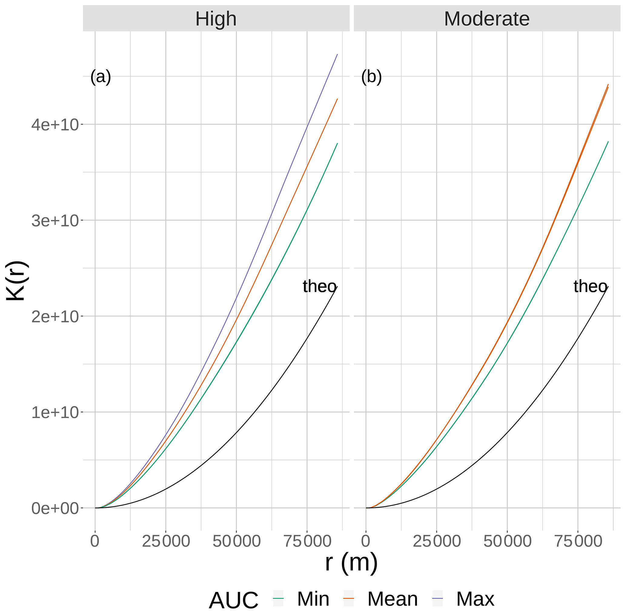
Figure 2 The results of Ripley's K function versus the neighborhood size (r) for eight static 2-D snapshot maps of DO from the bottom layer of the FVCOM-WASP simulation of 20–30 August 2002. The snapshots are defined in Table 1. Ripley's K values (lines) are shown for maps split into high (a) and moderate (b) sublethal areas and by AUC values with each panel. There are lines for the two minimum and single mean and maximum AUC values for the high sublethal area and for the minimum and to mean AUC areas for the moderate sublethal area. Some of the curves overlap and are not easily distinguished. The line labeled “theo” represents the relationship between Ripley's K and r for the theoretical condition when the spatial variability in sublethal DO cells is homogeneous.

2 Methods

2.1 FVCOM-WASP

Output from the coupled FVCOM-WASP model (Justić and Wang, 2014) was used with the FVCOM particle tracking module that was modified to simulate behavioral movement of individual fish. Individual fish were followed within the same 3-D grid that was used for hydrodynamics and the water quality modeling. The model domain covered the coastal GOM from Mobile Bay, Alabama, to Galveston Bay, Texas, and extended offshore to a depth up to 300 m with the water column divided into 30 sigma layers (Fig. 1, Wang and Justic, 2009). Sigma layers vary in their thickness across the model domain because the same number of layers are used from shallow to deep waters; individual fish locations are also available by depth that is computed from the sigma layers. The unstructured model grid allows higher resolution along the coast and an accurate representation of the GOM coastline. The FVCOM-WASP model has been previously calibrated to accurately represent the circulation and stratification on the shelf (Wang and Justic, 2009). Hourly DO from a 10 d simulation (20–30 August 2002) was used as the source for the 2-D and 3-D static and dynamic DO maps. The 20–30 August 2002 time period had a large hypoxic zone (∼ 16 000 km²) that showed variation at fixed locations on hourly and daily timescales. The bottom sigma layer from the 3-D FVCOM-WASP model output was used to create 2-D DO maps for simulating fish movement so that the DO values in the bottom layer were identical for the 2-D and 3-D maps.

2.2 Movement algorithms

Fish movement was simulated within the FVCOM-WASP grid by using a suite of algorithms that determined the velocities of individual fish in the horizontal plane (u and v) for 2-D and additionally using the vertical velocity (w) for the 3-D simulations (Rose et al., 2014; LaBone et al., 2019). The changes in fish position were calculated by updating their previous time step's positions on the grid with the newly computed velocities to obtain the new positions of the fish (Watkins and Rose, 2013; Rose et al., 2014). In 2-D, the equations are

$$\begin{array}{}\text{(1)}& {\displaystyle }x(t+\mathrm{\Delta }t)=x\left(t\right)+\mathit{u}\left(t\right)\cdot \mathrm{\Delta }t,\text{(2)}& {\displaystyle }y(t+\mathrm{\Delta }t)=y\left(t\right)+\mathit{v}\left(t\right)\cdot \mathrm{\Delta }t,\end{array}$$

where x and y were the fish positions on the model grid (distance in meters from bottom left-hand corner of grid), u and v are the velocities in the x and y directions, and Δt is the time step (15 min). The velocities u and v were calculated each time step as

$$\begin{array}{}\text{(3)}& {\displaystyle }\mathit{u}\left(t\right)=\text{ss}\cdot \cos \left(\mathit{\theta }\right(t\left)\right),\text{(4)}& {\displaystyle }\mathit{v}\left(t\right)=\text{ss}\cdot \sin \left(\mathit{\theta }\right(t\left)\right),\end{array}$$

where ss was the swimming speed (m s⁻¹) and θ was the swimming angle (radians) relative to the x axis. The swimming speed and swimming angle were computed differently among the algorithms, and which algorithm to use was selected based on the DO concentrations experienced by the fish. The collection of algorithms to model fish movement and exposure to DO were the same as used in previous analyses (LaBone et al., 2017, 2019).

2.2.1 Event-based movement

An event-based algorithm was used to choose among the various algorithms that computed swim speed and angle. There were four possible algorithms that an individual fish could use on a time step: neighborhood search (NS), Sprint, correlated random walk (CRW), and Cauchy CRW (CCRW). On each time step, two cues for DO-related movement were computed (e1 and e2), and these were used to select among three avoidance algorithms (NS, Sprint, and CRW) depending on the severity of hypoxia exposure. When none of the three DO-related algorithms for avoidance were selected, the individual used the default movement algorithm (CCRW) that was unrelated to DO conditions. The cuing variables e1 and e2 were binary variables (zero or one) computed on each time step (every 15 min) for each individual, with e1 being triggered when the DO concentration in the cell (exposure now) was less than 2 mg L⁻¹, and e2 was triggered when an individual's cumulative exposure to DO < 2 mg L⁻¹ exceeded a continuous 48 h. Thus, each individual had its own evolving time series of zero or one values for each cue (e1 and e2).

2.2.2 Neighborhood search

When the NS algorithm was selected by the event-based algorithm it was considered a tactical (immediate and urgent) response because the individual fish was about to be exposed to DO < 2 mg L⁻¹. The individual then searched the surrounding cells for the one with the lowest DO value and moved in the opposite direction at a swim speed twice the baseline (default) speed. The angle and swimming speed were calculated as

$$\begin{array}{}\text{(5)}& {\displaystyle }\begin{array}{rl}& \mathit{\theta }\left(t\right)=\mathrm{atan}\mathrm{2}\left(y\right(t)-yl(t),x(t)-xl(t\left)\right)\\ & +\mathrm{0.15}\cdot \mathrm{2}\mathit{\pi }(\mathrm{2}\cdot \text{ran}-\mathrm{1}),\end{array}\text{(6)}& {\displaystyle }\text{ss}=\mathrm{2}\cdot {\text{ss}}_{\mathrm{0}}\pm {\text{ss}}_{\mathrm{0}}\cdot \text{ran},\end{array}$$

where x(t) and y(t) are the current x and y coordinates, xl(t) and yl(t) are the coordinates of the center of the cell with the lowest DO, ss₀ is the default swim speed, and ran is a uniform random number. The first part of Eq. (5) (atan2), calculates the angle and the second part of the equation calculates a random component that adds some variability to the angle. The NS algorithm is efficient at avoiding hypoxia, but fish could get stuck in local maxima that were still hypoxic. The random component added to the swimming angle prevented most, but not all, fish from getting stuck at local hypoxic cells that were also the local maximum DO concentration.

2.2.3 Sprint

The Sprint algorithm was also considered a tactical response to hypoxia exposure and was selected when an individual fish spent too long in the hypoxic waters, often the result of being stuck at local hypoxic maxima from which the NS algorithm could not successfully move fish to non-hypoxic waters. If the fish spent more than 48 continuous hours in hypoxic conditions, the fish would swim quickly (3 times the default speed) in a straight line out of the hypoxic zone going in the direction the fish last traveled. The angle and swimming speed were calculated as

$$\begin{array}{}\text{(7)}& {\displaystyle }\mathit{\theta }\left(t\right)=\mathit{\theta }(t-\mathrm{\Delta }t),\text{(8)}& {\displaystyle }\text{ss}=\mathrm{3}\cdot {\text{ss}}_{\mathrm{0}}.\end{array}$$

The fish used Sprint on successive time steps until it exited the hypoxic zone, when its continuous exposure to hypoxia was reset back to zero.

2.2.4 CRW

CRW was a biased random walk algorithm (Kareiva and Shigesada, 1983) used for a strategic response to hypoxia. A strategic response is considered a response to hypoxia exposure but when the exposure is not immediate (like with tactical) but rather had occurred in the recent past. CRW, as a strategic response, typically followed the tactical NS response because once the immediate threat of exposure was gone, there was still some memory of the immediate exposure and the individual was likely in an area where there was hypoxia. The CRW algorithm had fish continue to swim away (at the relatively slower default speed) from hypoxic areas after NS enabled the fish to exit hypoxic conditions. CRW used the velocities from the previous time step to calculate the angle and calculated a random speed:

$$\begin{array}{}\text{(9)}& {\displaystyle }\begin{array}{rl}& \mathit{\theta }\left(t\right)=\mathrm{atan}\mathrm{2}\left(\mathit{v}\right(t-\mathrm{\Delta }t),\mathit{u}(t-\mathrm{\Delta }t\left)\right)\\ & +\mathrm{0.05}\cdot \mathrm{2}\mathit{\pi }\cdot (\mathrm{2}\cdot \text{ran}-\mathrm{1}),\end{array}\text{(10)}& {\displaystyle }\text{ss}={\text{ss}}_{\mathrm{0}}\pm \mathrm{0.3}\cdot {\text{sss}}_{\mathrm{0}}\cdot \text{ran}.\end{array}$$

The first half of Eq. (9) (atan2( )), are the velocities from the previous time step and the second part of the equation is a random component to add variation to the angle.

2.2.5 Default

CCRW was the random walk algorithm used as a default movement in the model and is a more complicated biased random walk than CRW (Wu et al., 2000). The magnitude and direction of the bias can be controlled by choosing the turning angle from a non-uniform, wrapped Cauchy distribution. The turning angle and swimming speed were calculated by

$$\begin{array}{}\text{(11)}& \begin{array}{rl}& \mathit{\theta }\left(t\right)=\mathit{\theta }(t-\mathrm{\Delta }t)+\mathrm{2}\cdot \mathrm{atan}\\ & \left[{\displaystyle \frac{(\mathrm{1}-\mathit{ϵ})}{(\mathrm{1}+\mathit{ϵ})}}\cdot \tan \left(\right(\text{ran}-\mathrm{0.5})\cdot \mathit{\pi })\right]+{\mathit{\theta }}_{\mathrm{m}},\end{array}\end{array}$$

$$\begin{array}{}\text{(12)}& \text{ss}={\text{ss}}_{\mathrm{0}}\pm \mathrm{0.3}\cdot {\text{ss}}_{\mathrm{0}}\cdot \text{ran},\end{array}$$

where ϵ determines the shape of the wrapped Cauchy distribution and θ_m determines the center of the distribution. θ(t-Δt) is the previous angle and the 2⋅atan[] + θ_m is the turning angle. Higher values of ϵ result in more correlation and less randomness to the direction of the fish. The value assigned to θ_m determined the bias in whether the individual tended to turn left or right.

2.2.6 Reflective boundary

Reflective boundary was an application of the NS algorithm used to reflect fish back into the model domain. Reflective boundary was used outside of the event-based algorithm and was applied after all of the other algorithms for fish movement were applied and the individual was placed in its new location. The reflective boundary algorithm would be triggered when a fish was determined to have moved outside of the model domain. The fish was moved back to its position at the start of the time step, and then the surrounding cells were searched and the fish moved to the cell with the fewest boundaries. The angle was calculated as

$$\begin{array}{}\text{(13)}& \begin{array}{rl}& \mathit{\theta }\left(t\right)=\mathrm{atan}\mathrm{2}\left(yl\right(t)-y(t),xl(t)-x(t\left)\right)\\ & +\mathrm{0.15}\cdot \mathrm{2}\mathit{\pi }\cdot (\mathrm{2}\cdot \text{ran}-\mathrm{1}),\end{array}\end{array}$$

where the values are the same as Eq. (5). The only change in the calculation of θ as compared to NS was the order of coordinate values in the atan2 function. Speed was calculated using the default swim speed (ss₀).

2.3 Algorithm selection

The event-based algorithm chooses the movement algorithm that has the highest utility for each time step. Utilities are used to represent the costs and benefits that a particular behavior has on an animal's fitness (Anderson, 2002). For our purposes of avoidance of low DO, we only considered that avoiding hypoxia was critical to fitness. In evaluating the different algorithms, we did not factor in the costs of avoiding hypoxia or how decisions would affect growth, mortality, or reproduction. We computed three utility values for each time step based on the probabilities of two events indicative of immediate (e1) and prolonged (e2) exposure occurring:

$$\begin{array}{}\text{(14)}& {\displaystyle }{U}_{\text{NS}}\left(t\right)={\text{util}}_{\text{NS}}\cdot {\text{prob}}_{\text{NS}}\left(t\right),\text{(15)}& {\displaystyle }{U}_{\text{sprint}}\left(t\right)={\text{util}}_{\text{sprint}}\cdot {\text{prob}}_{\text{sprint}}\left(t\right),\text{(16)}& {\displaystyle }{U}_{\text{CRW}}\left(t\right)={\text{util}}_{\text{CRW}}\cdot {\text{prob}}_{\text{CRW}}\left(t\right),\end{array}$$

where util_i is the intrinsic utility and prob_i is the probability of a triggered event. The intrinsic utility is the weight each algorithm has in the utility calculation. Tactical algorithms have a higher weight than default or strategic algorithms and thus are preferentially chosen. The probability of an event being triggered was calculated for NS and CCRW using the event of immediate exposure (e1):

$$\begin{array}{}\text{(17)}& {\displaystyle }\begin{array}{rl}& {\text{prob}}_{\text{NS}}\left(t\right)=(\mathrm{1.0}-{\text{mem}}_{\text{NS}})\cdot \text{e1}\left(t\right)\\ & +{\text{mem}}_{\text{NS}}\cdot {\text{prob}}_{\text{NS}}(t-\mathrm{\Delta }t),\end{array}\text{(18)}& {\displaystyle }\begin{array}{rl}& {\text{prob}}_{\text{CRW}}\left(t\right)=(\mathrm{1.0}-{\text{mem}}_{\text{CRW}})\cdot \text{e1}\left(t\right)\\ & +{\text{mem}}_{\text{CRW}}\cdot {\text{prob}}_{\text{CRW}}(t-\mathrm{\Delta }t).\end{array}\end{array}$$

The probability for Sprint used event two (e2):

$$\begin{array}{}\text{(19)}& \begin{array}{rl}& {\text{prob}}_{\text{sprint}}\left(t\right)=(\mathrm{1.0}-{\text{mem}}_{\text{sprint}})\cdot e\mathrm{2}\left(t\right)\\ & +{\text{mem}}_{\text{sprint}}\cdot {\text{prob}}_{\text{sprint}}(t-\mathrm{\Delta }t).\end{array}\end{array}$$

The three probabilities are running averages of present and recent past hypoxia exposures and allow for the fish to have some memory of past events. The utilities on each time step were then compared and the algorithm with the largest utility value that exceeded a minimum threshold was selected. If none of the calculated utilities were larger than the threshold (hypoxia exposure was not imminent and had not occurred in the recent past), then the default behavior was used. Parameters for Eqs. (14) to (19) are given in Table 2.

Table 2 Parameter values for the four movement algorithms used to simulate avoidance of low DO and the default behavior of individual fish.

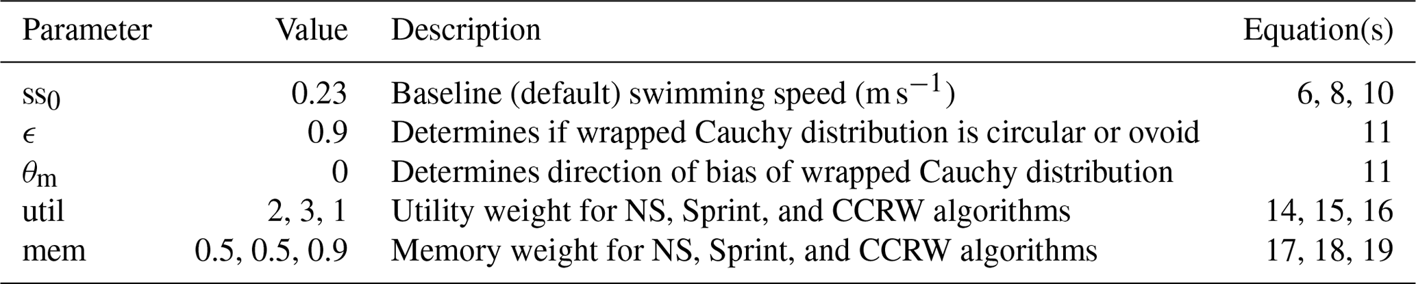
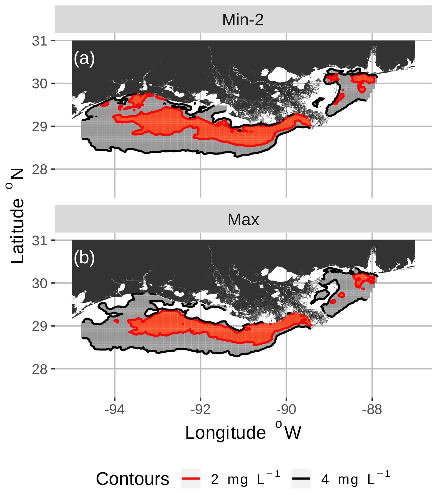
Figure 3 Spatial maps of bottom DO showing the 2 and 4 mg L⁻¹ contours for two of the eight snapshots from the FVCOM-WASP simulation of 20–30 August 2002. The snapshots are defined in Table 1. Snapshot Min-2 (a; row 2 in the Table) is moderate sublethal area and minimum AUC, and snapshot Max (b; row 8 in the Table) is high sublethal area and maximum AUC. Areas in white outside the 4 mg L⁻¹ line are normoxic.

2.4 Selection of static DO snapshots

Eight static DO snapshots were selected from the 240 hourly snapshots simulated during the 10 d (20–30 August 2002) FVCOM-WASP simulation (Table 1). For each snapshot, a 2-D map and a 3-D map of DO were created. The snapshots were selected based on a combination of the total area of sublethal DO and the degree of spatial variability in DO on each of the 240 2-D maps. Area based on the full range of sublethal concentrations (DO of 2–4 mg L⁻¹), and also the hypoxic area (DO < 2 mg L⁻¹) and normoxic area (DO > 4 mg L⁻¹) for reference and comparison, were computed for each hourly time step. Also for each of the 240 time steps (spatial maps of DO), Ripley's K function (Kest in R; https://www.rdocumentation.org/packages/spatstat/versions/1.63-3/topics/Kest, last access: 29 November 2020), with isotropic edge correction, was computed, which resulted in the plots of the statistic K versus r. Ripley's K is an estimation of the K function that accounts for maps with finite area and includes edge corrections. In our case, we have a 2-D spatial map of cells that are either hypoxic, sublethal, or normoxic. We computed the Ripley's K based on whether cells were sublethal or not. Ripley's K measures the number of extra sublethal cells (above that expected under randomly distributed sublethal cells) within a fixed distance (r, in meters) of a randomly chosen cell. Thus, Ripley's K used here is a method for quantifying the spatial distribution of sublethal cells on a map compared to the sublethal cells showing complete spatial randomness (CSR). As an aid in interpretation, our computed Ripley's K was compared to the theoretical value expected if the sublethal cells were spatially homogenous (K_theo; Fig. 2). If our computed K is less than K_theo, then the sublethal cells are spatially dispersed and sublethal cells are, on average, farther apart than expected compared to a random distribution. If our computed K for a map is greater than K_theo, then there is clustering of sublethal cells and sublethal cells generally occur closer together (clumped) than expected under randomness (Brunsdon and Comber, 2015). To obtain a single value for a map as an indicator of spatial variability so we could easily compare spatial variability across the 240 maps, we used the area under the curve (AUC) relating Ripley's K to r for each map. By using AUC that summarizes over a wide range of neighborhood sizes, larger AUC values imply the map has greater spatial variability (more clumpiness) in its distribution of sublethal DO concentrations.

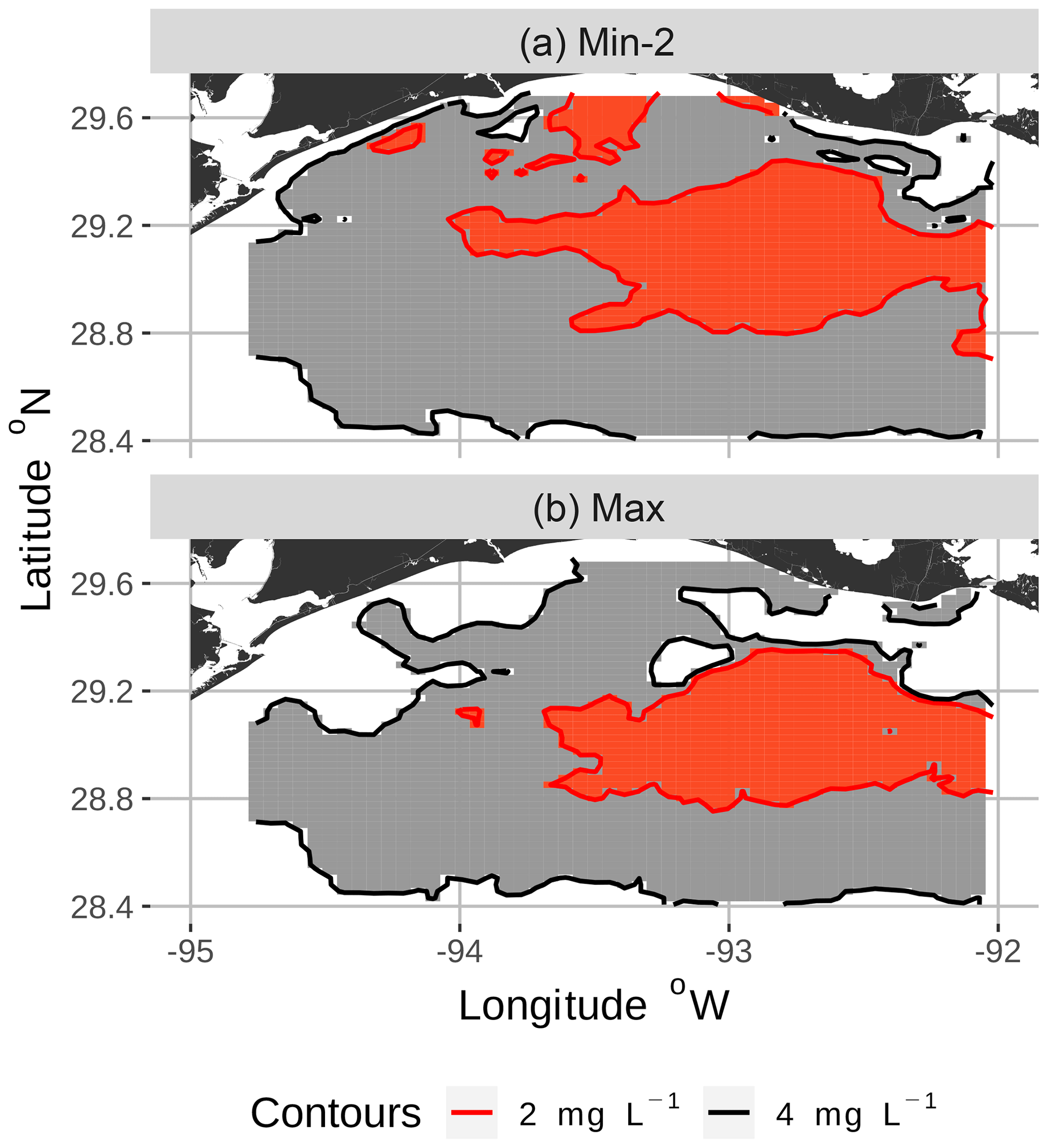
Figure 4 Zoomed-in view of spatial maps of bottom DO showing the 2 and 4 mg L⁻¹ contours for two of the eight snapshots from the FVCOM-WASP simulation of 20–30 August 2002. The snapshots are defined in Table 1. Snapshot Min-2 (a; row 2 in the Table) is moderate sublethal area and minimum AUC, and snapshot Max (b; row 8 in the Table) is high sublethal area and maximum AUC. Areas in white outside the 4 mg L⁻¹ line are normoxic.

To select the eight snapshots, we plotted AUC versus sublethal area and identified eight snapshots with moderate and high sublethal areas that corresponded to the minimum, mean, and maximum AUC values (Table 1). For moderate sublethal areas we selected two snapshots with minimum AUC and two snapshots with mean AUC; the maximum AUC was similar to the mean so no maximum was selected. For the high sublethal area case, two snapshots were matched with minimum AUC and single snapshots with mean and maximum AUC values (Fig. 2). The duplicate snapshots for a given AUC provide information on the variability of simulation results when two different maps have similar sublethal areas and AUC values. Figure 3 illustrates the spatial variability in DO using maps of sublethal DO for one of the minimum AUC (Min-2) snapshots for the moderate sublethal area and another for the maximum AUC (Max) with the high sublethal area. The larger area of sublethal concentrations is seen by the larger area of gray in Fig. 3b versus Fig. 3a. When we visually compared maps of low versus high AUC for the same sublethal area (high or moderate), differences in the degree of clustering of sublethal areas between low and high AUC values were not obvious. Figure 4 shows a blown-up area that illustrates the higher clumpiness and patchiness in sublethal DO when the AUC value is higher. The gray area in Fig. 4b (AUC of 1.67×109) shows more irregular boundaries, especially in the top left and right portions of the sublethal area, versus Fig. 4a (AUC of 1.33×109).

2.5 Design of simulations

Movement, and the associated exposure to DO, was simulated using 913 individual fish for 10 d on each of the eight static maps and the dynamic version. The number of fish was determined by placing a regular grid of fish locations onto the model domain and removing any that were assigned to land cells. The starting positions of the individuals were determined by using an algorithm that had fish move towards a preferred temperature (LaBone et al., 2017). Fish movement was simulated for several days until the temperature-seeking movement algorithm reached steady state with fish gathered along the 26 ^∘C contour line that was specified as their optimal temperature. This enabled initial starting locations to be spread out over the domain while preserving a relatively realistic initial spatial distribution expected without hypoxia. Simulations were done for the 2-D and 3-D maps and for good and poor avoidance competency. Good avoidance used the NS as described, while poor avoidance competency was achieved by changing the 0.15 value in Eq. (5) to 0.5, resulting in a much wider randomly generated direction of movement during avoidance. Fish positions were updated every 15 min, and DO in the dynamic maps changed every hour. We present the results for the 2-D set of maps; similar patterns of spatial variability of effects on exposure were obtained for the 3-D set of maps (Supplement). Movement parameters were set to values typical for croaker and related species (Table 2). Croaker is an abundant demersal-oriented fish in coastal waters of the northern GOM, especially in coastal waters off of Louisiana where hypoxia occurs annually. Extensive laboratory and field data available for DO effects on croaker have been previously used to specify realistic values for movement-related parameters (Rose et al., 2018b, a; LaBone et al., 2017, 2019).

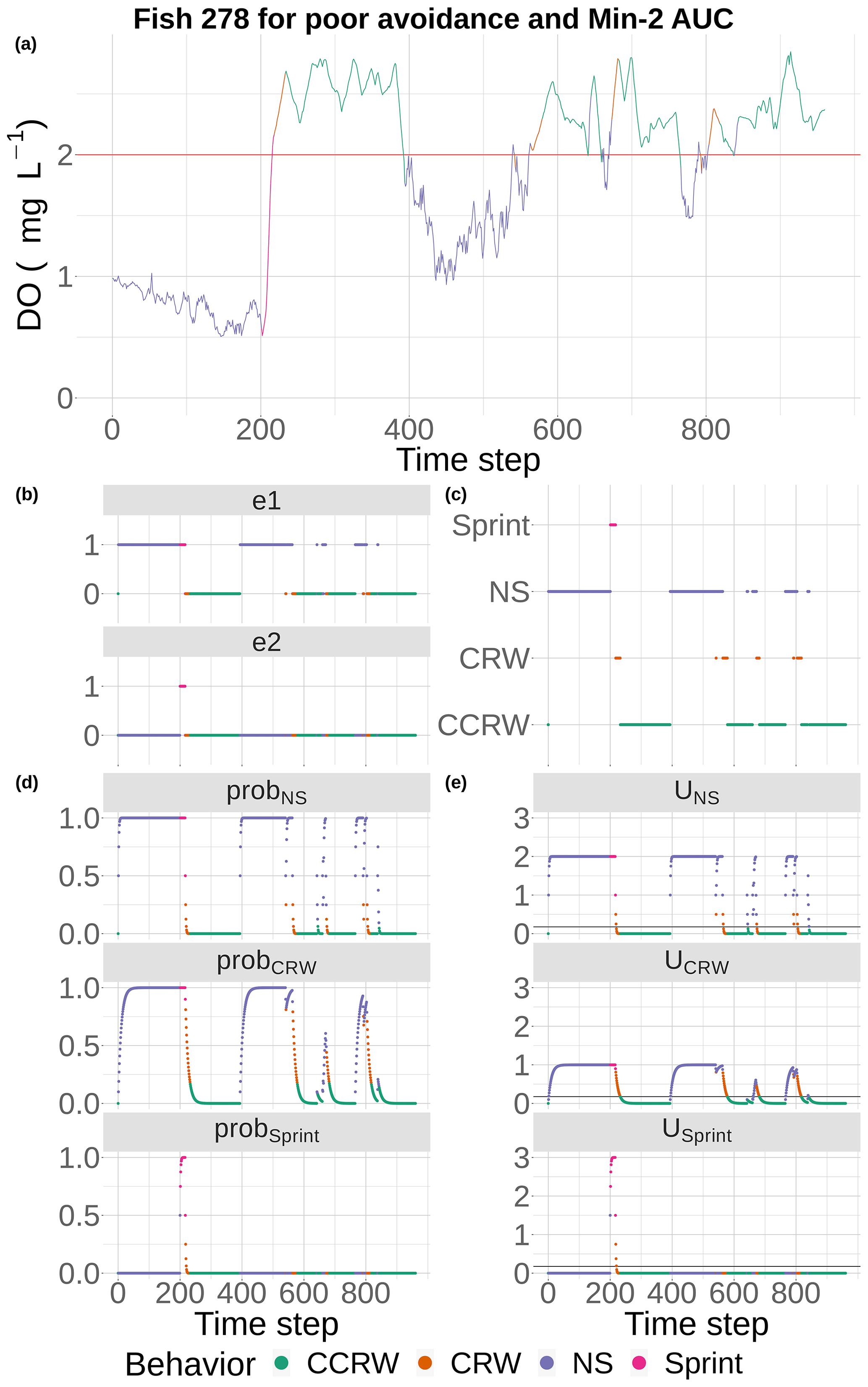
Figure 5 DO experienced and the component calculations used by the event-based algorithm to select movement algorithms at every 15 min time step for fish 278 under the conditions of poor competency and minimum AUC (Min-2) maps with moderate sublethal area. DO is used each time step (a) to determine e1 and e2 (b), with e1 used to compute the probabilities for NS (tactical) and CRW (strategic) avoidance and e2 used to compute the probability for Sprint (d). These probabilities are used to compute utilities for the three algorithms each time step, (e) and the algorithm with highest utility above a minimum threshold is selected to be used for movement for that time step (c). If none of the three avoidance-related algorithms are selected, then a fourth algorithm (CCRW) that is unrelated to DO concentration is used.

Model outputs of fish locations and DO experienced every 15 min were analyzed to determine how spatial variability in DO affected exposure to hypoxia and sublethal DO concentrations. To illustrate the movement behavior, we show the detailed movement calculations (e1, e2, and the three probabilities and utilities) for a single fish for poor competency on a single static map (Min-2 of moderate sublethal area) and the movement tracks and DO experienced for four individual fish for good and poor avoidance on two of the static DO snapshots. The DO experienced was color coded to show which movement algorithm was being used over time.

Exposure of all individuals was summarized over the 10 d for each fish by their cumulative exposure, which was calculated as the sum of the number of 15 min time steps (expressed as days) each fish was exposed to DO less than 2 mg L⁻¹. Cumulative exposure to sublethal conditions was calculated the same as the exposure to hypoxia, except the overall sublethal range of 2–4 mg L⁻¹ (sublethal) was subdivided into 2–3 mg L⁻¹ and 3–4 mg L⁻¹, and each of these was considered the “exposed”. We show plots of the cumulative exposure of all individual fish and also boxplots that summarize cumulative exposures over all fish. Outlier values were displayed in the box plots as points beyond the whiskers of the plot and were identified as values outside 1.5 ⋅ IQR (interquartile range). The outliers are considered extreme but usable values, as they were not questionable or suspicious “outlier” values in the statistical sense, and were therefore included in all analysis of model outputs. Another summary of the exposure output was the percentage of fish on each time step between 2–3 mg L⁻¹. We focus on the 2–3 mg L⁻¹ range for the sublethal analysis in this paper because it would have the most ecological effects on individuals (just above lethality) and the results for 3–4 mg L⁻¹ were consistent with 2–3 mg L⁻¹ but showed less overall variation and so the patterns were less clear. R was used for all statistical analysis and graphs (R Core Team, 2019).

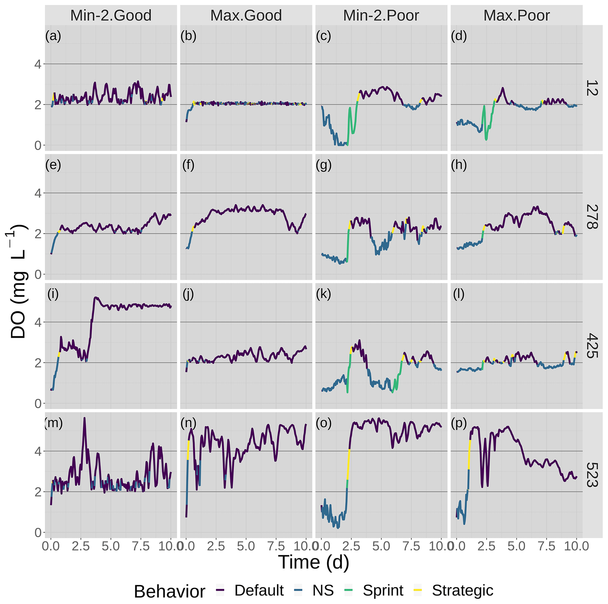
Figure 6 Time series of DO experienced by the four fish shown in Fig. 7 over the 10 d of the model for good and poor avoidance and the two snapshot DO maps (Min-2 for moderate sublethal and Max for high sublethal area). The color of the lines denotes the movement algorithm that each individuals was using. Black lines denote the thresholds for hypoxia (2 mg L⁻¹) and the upper value (4 mg L⁻¹) considered for sublethal concentrations.

3 Results

3.1 Hypoxia avoidance in 2-D

Fish movement was a mix of the different behaviors, depending on the DO conditions they encountered (Figs. 5 and 6). Our example fish (Fig. 5) was immediately exposed to hypoxia that triggered the NS tactical avoidance (via e1) and also showed a slower rising utility for the CRW (strategic) as the fish’s past exposure was considered. When the fish was unable to avoid waters with DO < 2 mg L⁻¹ for 2 d (time step = 192, Fig. 5a), Sprint got invoked (Fig. 5b, c). Once the fish entered waters with DO > 2 mg L⁻¹ using Sprint, the utilities for both NS and CRW avoidance movement quickly returned to zero as exposures to DO > 2 mg L⁻¹ accumulated (Fig. 5e). The fish then used default (CCRW) while moving among cells with DO > 2 mg L⁻¹ (Fig. 5c). At time step 400, the fish wandered into water with DO < 2 mg L⁻¹, causing the utilities for NS and CRW to rise (Fig. 5e) and triggering NS for an extended time period (time steps 475 to 600, Fig. 5c) as the fish moved around trying unsuccessfully to avoid waters with DO < 2 mg L⁻¹. Once NS enabled the fish to move to waters with DO > 2 mg L⁻¹, CRW would briefly get triggered because of its history of exposure (Fig. 5c). Several more times the pattern of NS and CRW (both avoidance) were triggered (Fig. 5c, e), mostly keeping the fish in waters with DO > 2 mg L⁻¹, except for a few brief time periods (Fig. 5a). While the fish generally avoided hypoxia after the initial exposure and during the one extended period of hypoxia exposure (time steps 475 to 600), the fish was then always exposed to sublethal levels (2–4 mg L⁻¹) throughout the 10 d.

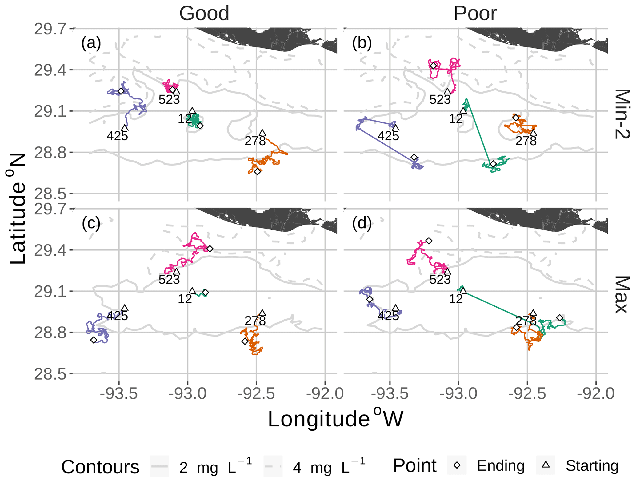
Figure 7 Movement tracks taken by four fish for good and poor hypoxia avoidance (left versus right) and two snapshots (Min-2 for moderate sublethal area and max AUC for high sublethal area). All four fish start (triangle symbol) in the hypoxic zone. These are the same maps as shown in Fig. 3, but here they only show a portion of the model grid.

DO experienced and fish trajectories (Figs. 6 and 7) illustrated how a fish with good avoidance used NS (mostly straight path with some randomness) to escape the hypoxic zone, while several of the fish with poor avoidance (higher randomness) had to use Sprint (perfectly straight path) after spending 48 h in hypoxic conditions. Several of the selected fish used a mix of all four algorithms (all fish in Min-2 with poor competency), while other individuals used two or fewer algorithms that were dominated by default movement. The exposure patterns and variability in DO experienced also varied among individuals, even though these were maps with fixed spatial distributions of low DO. For example, individual no. 12 (Fig. 6b), after escaping hypoxia exposure, was exposed to DO just above 2 mg L⁻¹ throughout, while other individuals on certain maps (e.g., 425 on Min-2 with good competence, Fig. 6i) eventually went to waters with DO > 4 mg L⁻¹.

3.2 Hypoxia exposure

Cumulative exposure of individuals to hypoxia was higher under the high sublethal area snapshots compared to the moderate sublethal snapshots, with good competence showing the greater difference between moderate and high. With good avoidance competency, almost all fish showed exposures of about 1–2 d for maps with high sublethal area (Fig. 8a), which were further reduced to almost no exposure to hypoxia for moderate sublethal area maps (Fig. 9a). Sublethal area was positively correlated with hypoxic area, while both were somewhat negatively related to normoxic area (Table 1). Poor avoidance resulted in much more similar exposures between high and moderate sublethal conditions (Figs. 8b and 9b), which reflected that the fish have more randomness to their avoidance movement that masks some of the differences between the moderate and high sublethal area maps. Because of the effects of Sprint being triggered after the first 48 h for some fish under poor competency, we also examined the results using days 3 through 10 (Supplement). The patterns in the results described for hypoxia exposure were less pronounced for the good competency results because there was little exposure to hypoxia after the first 48 h when fish moved out of hypoxia and were effective at avoiding further exposure. However, removing the effects of the initial triggering of Sprint for poor competency simulations only slightly lowered overall hypoxic exposure, as fish continued to be exposed to hypoxia intermittently but with similar percentage of individuals throughout the 10 d.

The effects of different degrees of spatial variability on hypoxia exposure were small. There was a weak suggestion that exposure to hypoxia decreased with increasing variability with the high sublethal area maps but increased with increasing variability for moderate sublethal area maps. This is seen by the tendency for exposure to decrease from left to right in each panel of Fig. 8, while exposure tended to increase from left to right in each panel of Fig. 9. This pattern of opposite effects of spatial variability on hypoxia exposure being dependent on the degree of sublethal area, which is weak here, will become more apparent when sublethal exposure is examined.

3.3 Sublethal exposure

The effects of spatial variability on cumulative sublethal exposure to 2–3 mg L⁻¹ of individuals showed higher exposure for high sublethal area (as expected – simply more possibility of exposure) and a tendency for opposite effects of variability between high and moderate sublethal areas. For poor avoidance and especially for good avoidance competency, there was a subtle but consistent shifting to lower exposures with increasing variability for high sublethal area (points shifting to lower values from top to bottom in Fig. 10), while there was a shifting to higher exposures for the moderate sublethal area maps (less open space near top of each plot, except for dynamic, in Fig. 11). The pattern of fish with ID values greater than 750 having higher exposures to sublethal DO in Figs. 10 and 11 was due to the how individuals were numbered in the simulation and how they related to where they were initially placed on the grid. High-numbered individuals were generally located closer to hypoxia and sublethal concentrations at the start of the simulations.

This opposite effect of variability was more apparent when the exposures of fish to 2–3 mg L⁻¹ was examined as the percent of all individuals. Under high sublethal area, the percent of fish exposed to 2–3 mg L⁻¹ decreased with increasing variability for both good competency (Fig. 12a) and poor competency (Fig. 12b). The green lines (min AUC, low variability) had the highest exposure, while the purple lines (max) and magenta lines (dynamic map) had the lowest exposures. For good competency, the averaged percent of individuals exposed to 2–3 mg L⁻¹ over the 10 d was 46 % and 47 % for the two min variability maps, 39 % for the mean map, and 37 % for the max map. A similar range (maximum minus minimum) of averaged percent exposed of about 8 % occurred with poor competency: 37 % and 38 % for min variability, 32 % for mean, and 30 % for the max map. In both cases, the percent exposure for the dynamic maps were within the values of their respective static maps (38 % for the good competency and 29 % for poor competency).

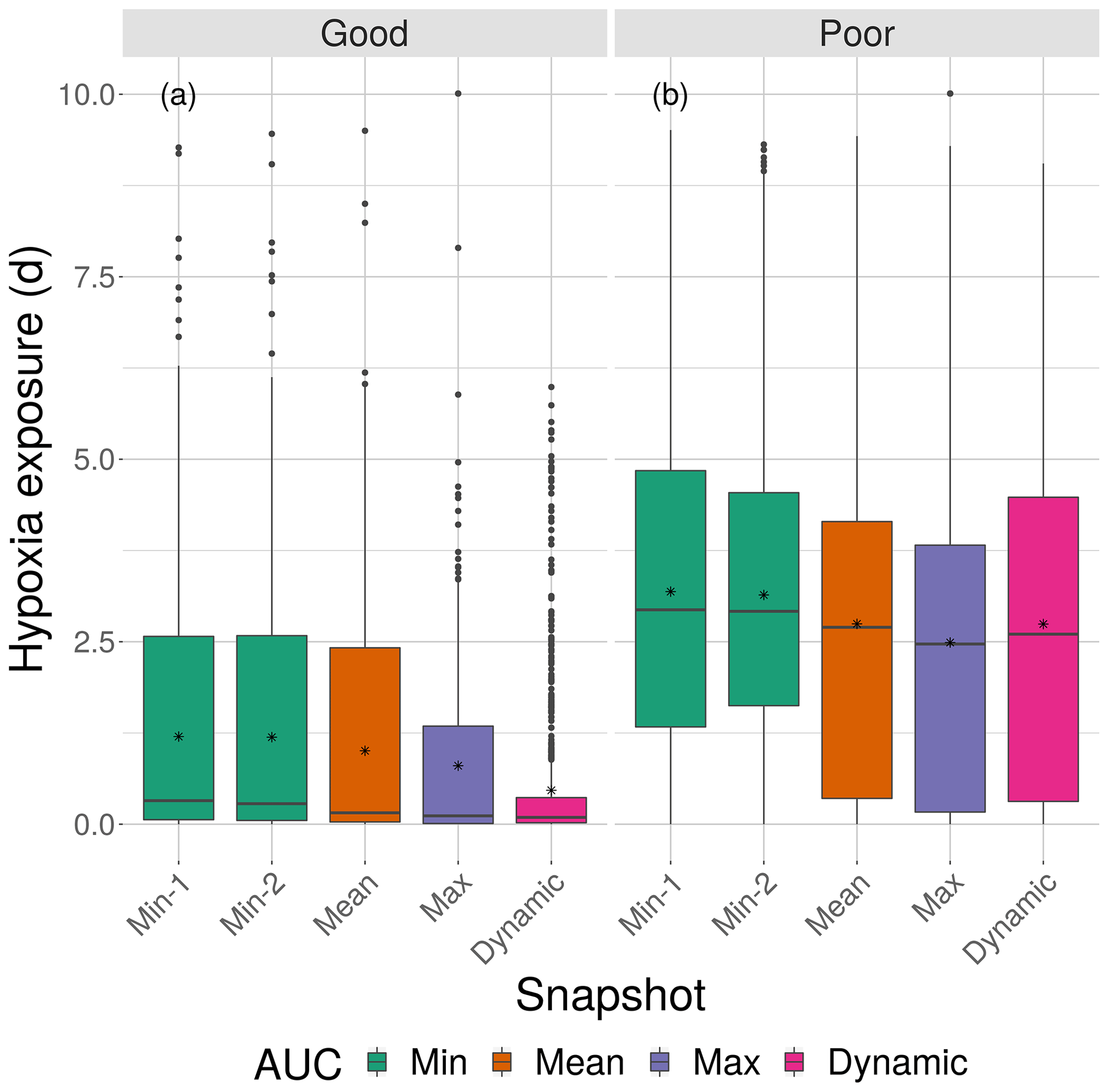
Figure 8 Boxplots of cumulative hypoxia exposure of all individuals (days) for good and poor competency on the four DO snapshot maps with high sublethal area. The cumulative exposure for the simulation using the dynamic map is also shown. The lower and upper lines of the boxplots show the 25th and 75th percentile value of cumulative exposure and the center line is the median. Individual fish values flagged as extreme values are shown as individual points. The star symbol denotes the mean.

The opposite pattern was predicted for the moderate sublethal area conditions (Fig. 13); percent exposed to 2–3 mg L⁻¹ increased, rather than decreased, with increasing variability. In Fig. 13, the green lines (2 min AUC maps) showed the lowest exposures while the orange line (mean AUC) and magenta line (dynamic) showed the highest exposures. For good competency, the averaged percent of individuals exposed to 2–3 mg L⁻¹ was 36 % for the two min variability maps and 40 % and 43 % for the mean maps, a range of about 8 %. For poor competency, there was little difference in percent exposed from min and mean maps: 28 % for the two min maps and 29 % for the two mean maps. This lack of a difference was also due to the inclusion of the first 2 d when exposure was similarly low on all of the maps due to Sprint, but the differences after day 2 were still not strong.

The opposite effects of spatial variability between moderate and high sublethal areas were maintained for 3-D simulations, and the effects were maintained, but smaller, for exposure to 3–4 mg L⁻¹. The patterns for exposure to 2–3 mg L⁻¹ were maintained after the first 48 h of exposures, so that Sprint was not overly influential on the patterns, and also under 3-D conditions, demonstrating the results were robust to including an option for vertical avoidance (see the Supplement). For both moderate and high sublethal areas, the opposite effects of spatial variability were similar but less apparent for exposure to 3–4 mg L⁻¹ because exposures in general showed less variation among simulations for 3–4 mg L⁻¹ (results not shown).

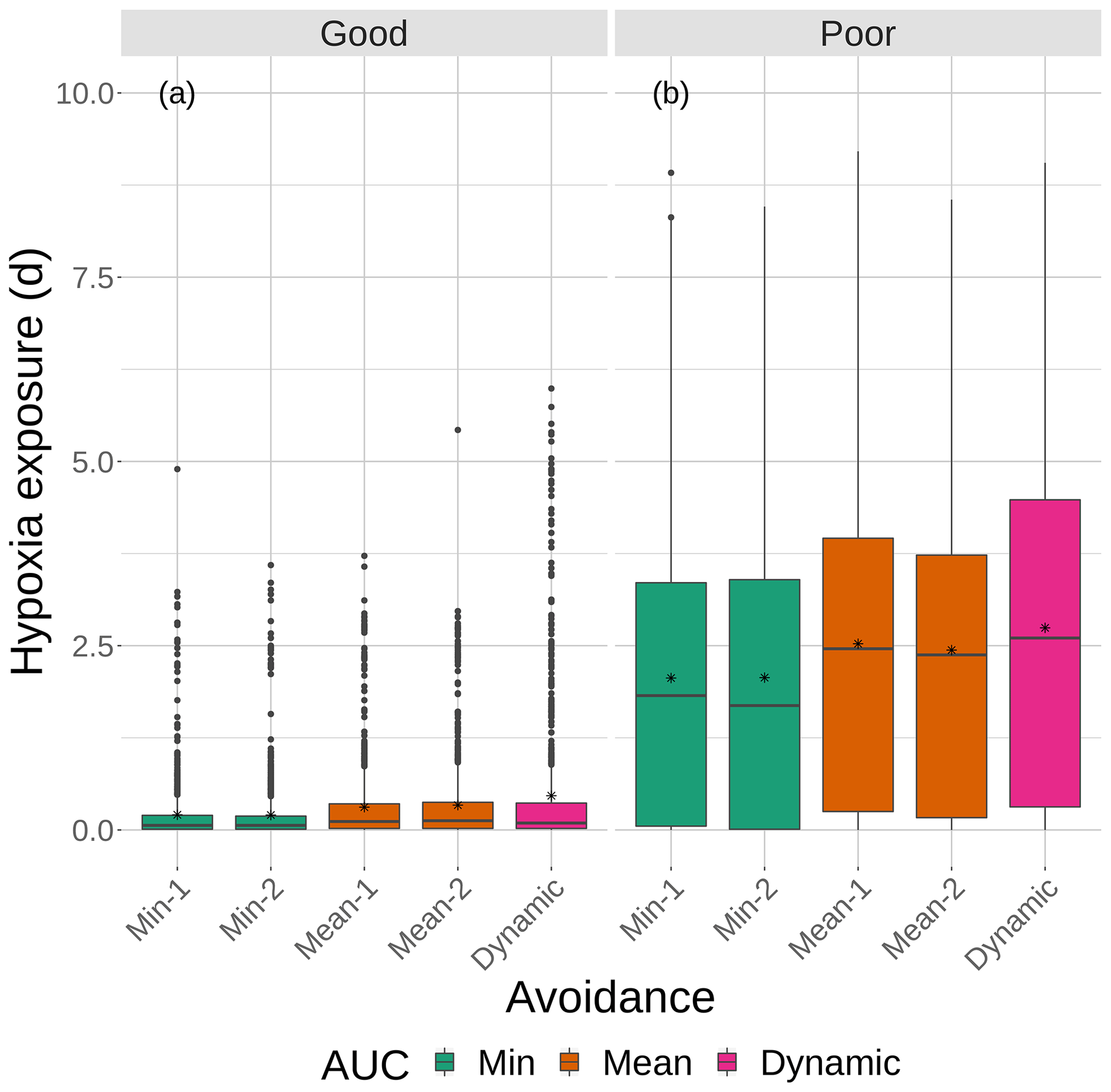
Figure 9 Boxplots of cumulative hypoxia exposure of all individuals (days) for good and poor competency on the four snapshot DO maps with moderate sublethal area. The cumulative exposure for the simulation using the dynamic map is also shown. The lower and upper lines of the boxplots show the 25th and 75th percentile value of cumulative exposure, and the center line is the median. Individual fish values flagged as extreme values are shown as individual points. The star symbol denotes the mean.

4 Discussion

The spatial variability of DO in the Gulf of Mexico, and likely in other places with chronic river-driven seasonal hypoxia, is patchier than we envisioned. As measurements become more resolved and hydrodynamic water quality models become more detailed, what was once considered a continuous area of hypoxia now reveals itself to have a much more spatial structure. The persistence at a location, the dissipation and reforming of hypoxia in response to weather events, local bathymetric influences (e.g., Virtanen et al., 2019), and other factors, all contribute to the spatial variability in the hypoxic and sublethal DO concentrations (Bianchi et al., 2010; Rabalais and Turner, 2019). The rather smooth looking earlier annual spatial maps obtained from monitoring data (e.g., Rabalais et al., 2001) are continually evolving into more irregular shapes with highly dynamic boundaries and patchiness (Zhang et al., 2009; Obenour et al., 2013; Justić and Wang, 2014). Further, while we focus on the hypoxic waters, most mobile organisms show avoidance behavior, making the dynamics of sublethal concentrations (often not avoided) highly relevant ecologically. Hypoxia causes mortality, which is a major consideration at the population level, but the population effects also depend on the fraction of the population that is exposed. Reduced growth, lowered fecundity, and indirect effects from displacement may have a less obvious influence on the population than mortality, but if a much larger percent of the population are exposed, these sublethal effects can lead to ecologically significant population-level responses that, in some cases, can exceed the effects from direct mortality (Rose et al., 2009). Fish movement, spatial variability in DO, and exposure to hypoxia and sublethal concentrations are complicated. However, knowing exposure is critical in order to make accurate predictions of the effects of low DO on individuals, which then can be scaled to the responses of populations and food webs (Rose et al., 2009, 2018b, a; De Mutsert et al., 2016). In this paper, we are using simulation methods to explore this issue of how spatial variability in DO would affect exposure of fish to hypoxia and sublethal concentrations of DO.

4.1 Exposure to sublethal DO

Our a priori intuitive thinking was that more spatially variable DO would lead to higher exposure to hypoxia. A fixed stable hypoxic area would allow most fish to avoid the area and minimize exposure once they have adjusted to the initial encounter. Patchy or clustered locations of hypoxia would mean that fish would have to continually deal with possible exposure and there would be many more opportunities for swimming into low DO water. We also assumed that because waters with sublethal DO levels would be associated (loosely adjacent) with hypoxia, more avoidance of hypoxia would also result in higher exposure to sublethal DO. If the patchiness was also dynamic in time, then that would seem to further increase the chances of encountering low DO water and thereby increase exposure even more. Our analysis reveals important details, nuances, and incorrect aspects of this intuitive (conceptual-level) view of how spatial variability in DO would affect fish exposure.

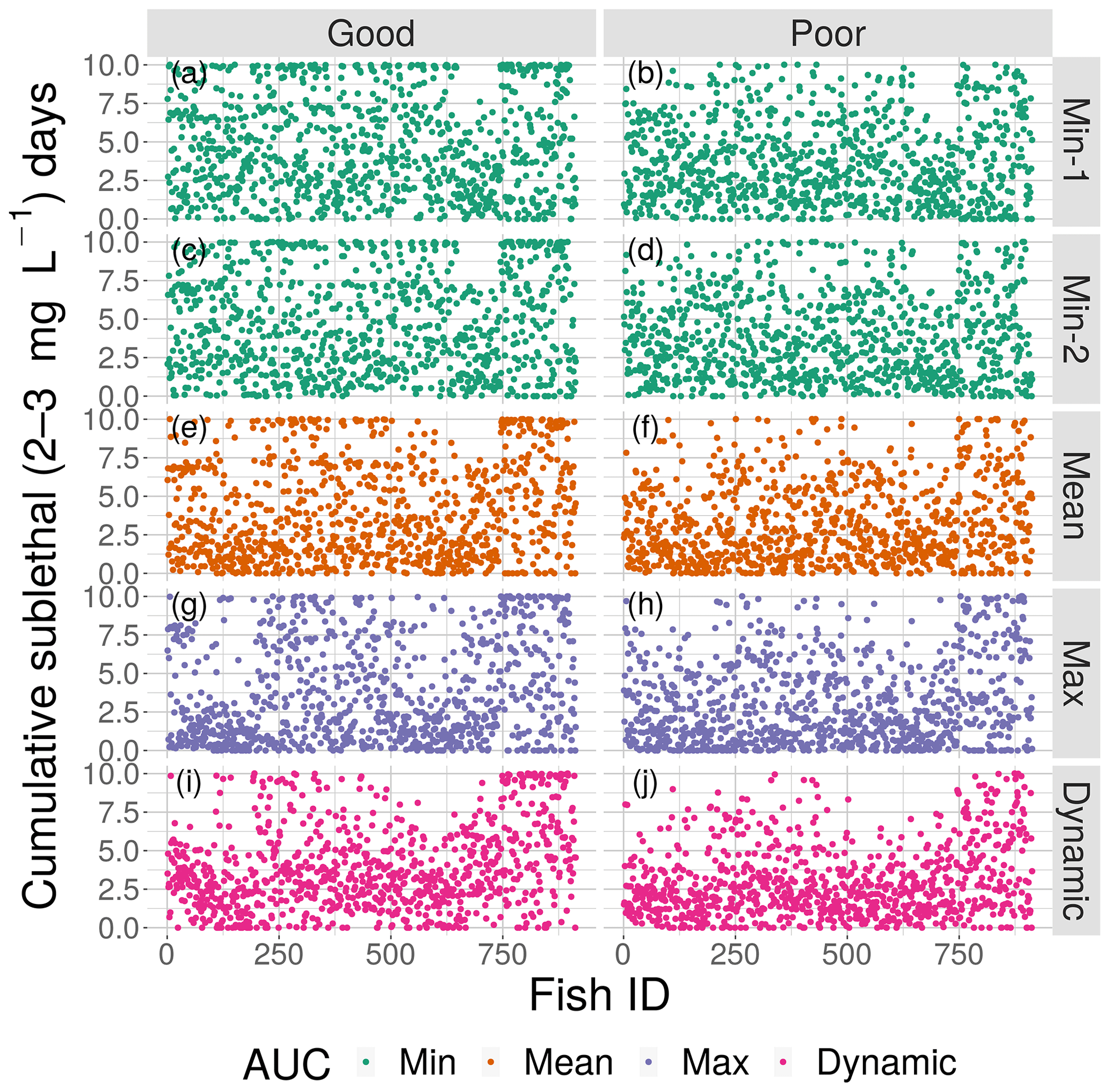
Figure 10 Cumulative exposure (days) of each individual fish to DO concentrations of 2–3 mg L⁻¹ for good (left) and poor (right) competency for each of the four snapshot DO maps with high sublethal area and the dynamic version. Maps within the same AUC category (the two “Min” maps) are shown with the same color.

Our refined view of how spatial variability affects exposure distinguishes between hypoxia and sublethal exposures and shows that effects of spatial variability on sublethal exposure can reverse depending on the areal extent of low DO waters. Model simulations showed that exposure to hypoxia was, as expected, greatly influenced by the swimming avoidance competency assumed for the fish. Given other conditions were the same, good competency (little randomness to avoidance response) resulted in less exposure to hypoxia than poor competency (left versus right panels in Figs. 8 and 9). Further, good competency essentially eliminated exposure to hypoxic conditions. Almost all exposure to hypoxia occurred in the first 24 to 48 h, and this was generally low (Fig. 8a). Beyond the initial exposures (i.e., using days 3–10), good competency resulted in near-zero exposure to hypoxia (see the Supplement). In contrast, exposure to hypoxia with poor competency showed persistent and relatively high exposure to hypoxia that occurred throughout the 10 d of the simulations (results not shown). Such persistent exposure occurred even when the effects of initial use of Sprint in the first 48 hours were eliminated (see the Supplement).

Despite the differences in exposure to hypoxia with good versus poor competency, both resulted in relatively high exposures to sublethal DO concentrations. Roughly, 30 % to 50 % of the individuals were exposed to 2–3 mg L⁻¹ and this occurred, except for the 48 h that triggered Sprint, throughout the 10 d of almost all of the simulations (Figs. 12 and 13). Interestingly, the percent of individuals exposed to 2–3 mg L⁻¹ was often somewhat higher (about 5 %–10 %) for good competency compared to poor competency. The reason is that good competency resulted in fewer individuals being exposed to hypoxia and so more individuals were available to be exposed to sublethal concentrations. If an individual was successful at avoiding hypoxia, they likely were then exposed to sublethal concentrations. Our results do not support the idea that fish with good avoidance behavior ameliorate the ecological effects of low DO. Rather, even fish with good avoidance abilities are exposed to sublethal concentrations and good avoidance may shift individuals from hypoxia to sublethal exposures rather than to no-effects. Our results also showed that this occurred when the fish were given the option to swim vertically to avoid hypoxia (see the Supplement). We need to accurately predict avoidance behavior in order to quantify the effects of hypoxia exposure on mortality and the effects of exposure to sublethal concentrations on growth and reproduction.

Figure 11 Cumulative exposure (days) of each individual fish to DO concentrations of 2–3 mg L⁻¹ for good (left) and poor (right) competency for each of the four snapshot DO maps with moderate sublethal area and the dynamic version. Maps within the same AUC category (min and mean) are shown with the same color.

The effects of spatial variability in DO on sublethal exposure were opposite depending on the degree of sublethal area. Exposure to 2–3 mg L⁻¹ decreased with increasing variability for maps with high sublethal area but increased with variability for maps with moderate sublethal area (reverse ordering of line colors between Figs. 12 and 13). One possibility is that our measure of spatial variability (Ripley's K, Fig. 2) did not capture variability but rather reflected some other feature of the DO concentrations (e.g., co-occurrence of sublethal with hypoxic areas) related to high versus moderate sublethal areas. Spatial maps of DO for different degrees of spatial variability did not show obvious and dramatic differences in the spatial patterns of sublethal DO concentrations (Fig. 3). Furthermore, we used an aggregate measure (area under the curve) to further summarize the Ripley's K values, which generates a series of values for increasing spatial neighborhoods (K versus r in Fig. 2). With our maps, showing Ripley's K values above the theoretical value for our maps implies the “patches” of sublethal DO concentrations are all more clustered than randomly distributed. If our summarization of Ripley's K values is valid, then higher AUC values suggest that the patches of sublethal concentrations are more clustered over a range of spatial scales. The similarity of exposures for “replicate” maps (i.e., similar AUC values) show that our patterns of exposure with variability are robust. If the AUC values reflect overall spatial variability, then our results clearly demonstrate that quantifying exposure is a complicated overlaying of spatial DO with moving fish that depends on relatively subtle differences in the amount of low DO area, its spatial distribution, and the avoidance abilities assumed for the fish movement behavior.

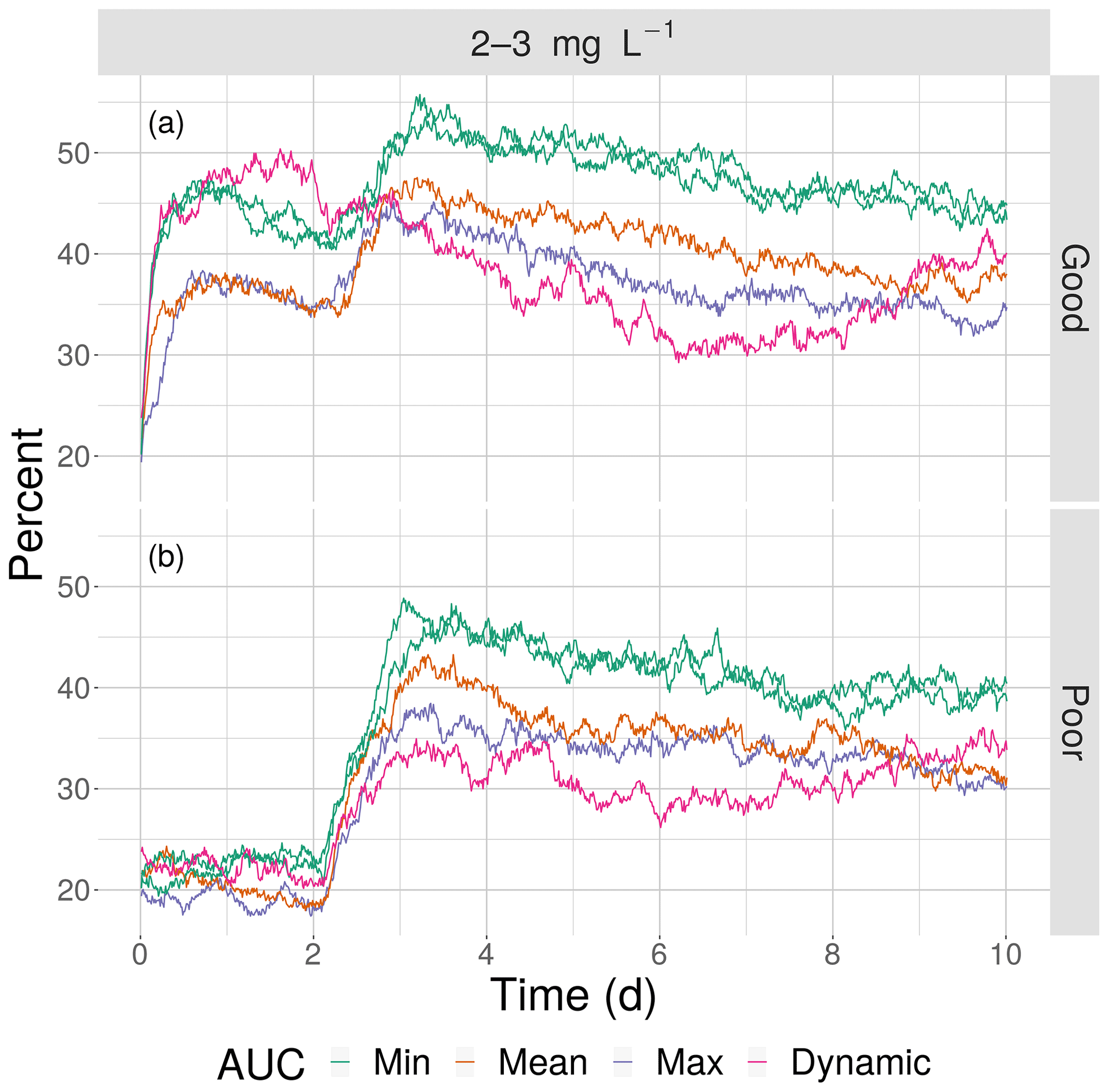
Figure 12 The percentage of fish exposed to DO of 2–3 mg L⁻¹ for good (a) and poor (b) competency for the four snapshot maps with high sublethal area and the dynamic version. Maps within the same AUC category (“Min”) are shown with the same color.

We hypothesize that spatial variability in DO has opposite effects on exposure depending on the degree of sublethal area due to effects of how individuals encounter the patches of sublethal concentrations as a result of avoidance of hypoxia. With high sublethal area there is also high hypoxic area (Table 1) and thus individuals frequently used avoidance. Normoxia was always greater than 55 % of the area, compared with 12 %–15 % for hypoxia and 23 %–30 % for sublethal. These active individuals avoid hypoxia, but with higher clustering of sublethal areas there are locations (refuge areas adjacent to hypoxic areas) to move to that are normoxic (i.e., not sublethal). With relatively low Ripley's K (lower spatial variability), the patches of sublethal concentrations are more evenly distributed, and thus fish avoiding hypoxia are more likely to encounter a sublethal patch.

The opposite pattern for moderate sublethal area is also about encounters. Rather than clustering creating refuges when there is high degree of sublethal area, clustering with moderate sublethal area creates more opportunities for individuals to encounter the relatively rare sublethal concentrations. With relatively low Ripley's K values, the same moderate sublethal area consists of dispersed patches. This creates many opportunities for individuals that avoid hypoxia to locate in high DO cells. We might expect that higher spatial variability in the case of moderate sublethal area results in a subset of individuals inhabiting areas with hypoxia associated with sublethal concentrations, and thus some individuals should show persistent exposure to sublethal concentrations. Our hypothesis is speculative and should be investigated further using designed simulation experiments and by following the DO experienced over time across many individuals. Additional statistical analysis of the spatial heterogeneity in sublethal areas beyond Ripley's K is also needed to better understand the spatial features that drive the changes in exposure between high and moderate sublethal area maps.

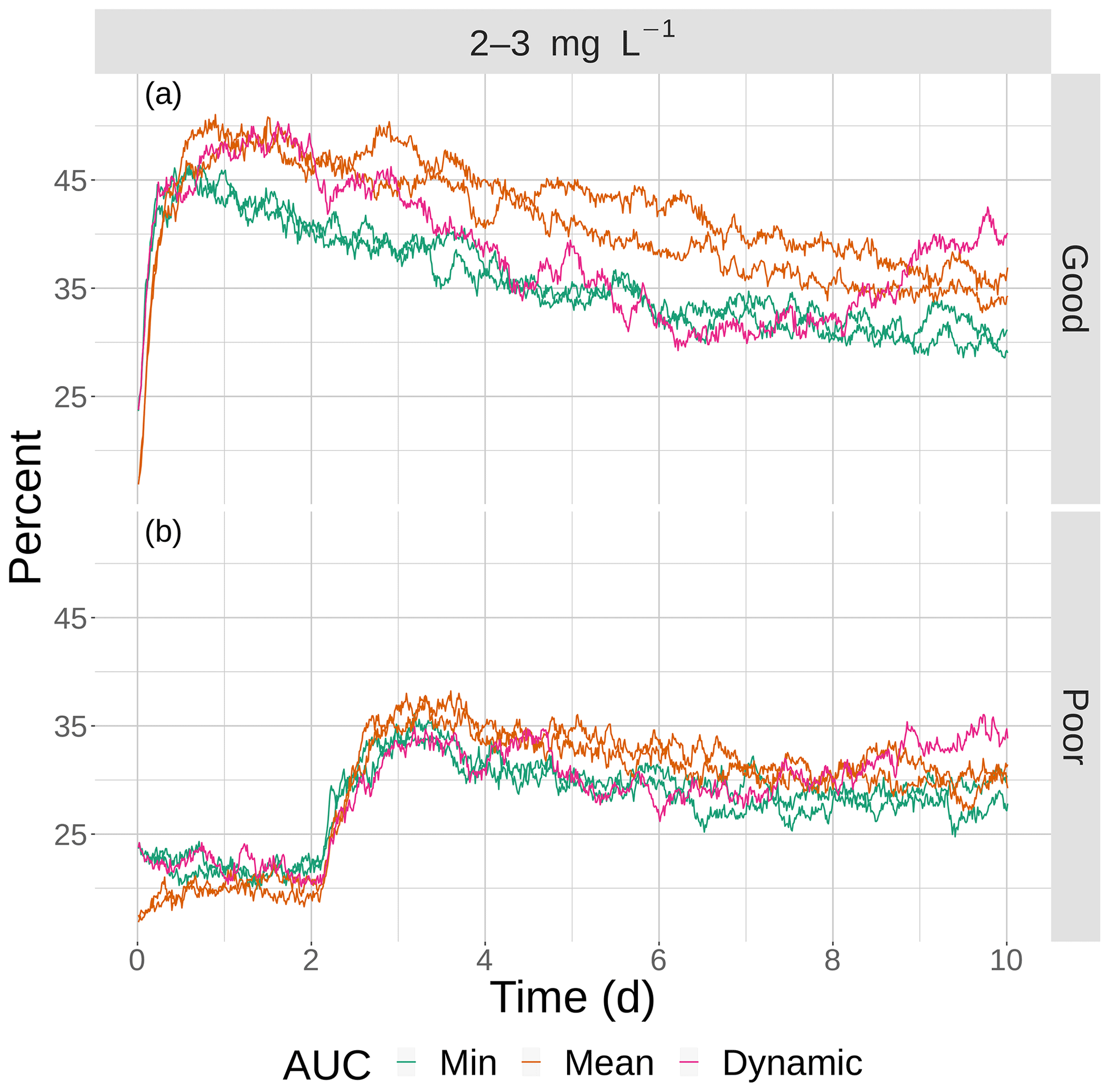
Figure 13 The percentage of fish exposed to DO of 2–3 mg L⁻¹ for good (a) and poor (b) competency for the four snapshot maps with moderate sublethal area and the dynamic version. Maps within the same AUC category (min and max) are shown with the same color.

We initially considered that the dynamic map would generate exposure results acting as the most spatially variable map. Not only were there differences among cells in the dynamic maps, but the DO in each cell also changed every hour. Sublethal exposure with the dynamic maps did, as expected, have the lowest exposure for the high sublethal area (magenta lines in Fig. 12) that continued the trend of decreasing exposure with increasing variability. However, the sublethal exposure for the dynamic maps with the moderate sublethal area was inconclusive (Fig. 13). The line for the dynamic map crossed several times with the lines for min and mean AUC maps in both the good and poor competency simulations. When viewed more generally, the sublethal exposures with the dynamic maps were all generally within the range of exposures predicted over the static maps, confirming that our results for static maps also apply to the more realistic situation of temporally and spatially varying DO maps. Our results are not sufficient to determine how temporally dynamic DO combines with the spatial variability in DO to affect sublethal exposures. However, it is encouraging that our results suggest that knowing about spatial variability of low DO concentrations can enable realistic estimation of exposure even under temporally dynamic conditions. Additional simulations that use DO seascapes with known combinations of spatial and temporal variation are needed to further untangle the effects of spatial and temporal variation in DO on exposure.

Another result from our analysis that complicates quantifying exposure to hypoxia and sublethal DO concentrations is the very high level of variability in exposure predicted among individuals (Figs. 10 and 11). Given simulations were for 10 d with individuals released within a region of the hypoxic zone and with static DO maps, one might expect exposure (either low or high) would be similar among individuals. Yet, even under these conditions of exposure with an assumed competency and static DO conditions, inter-individual variation in exposure was substantial. The effects of constant and time-varying exposures on growth and fecundity can be nonlinear (e.g., threshold or accelerating effects) at the level of individual (McNatt and Rice, 2004; Neilan and Rose, 2014) and hypoxia effects can be interactive with other factors and stressors (McBryan et al., 2013; Breitburg et al., 2019). Thus, using an exposure averaged over individuals (and/or averaged over time such as weekly) to assess ecological responses will likely underestimate effects that occur with exposures to low DO. Coiro et al. (2000) showed that the growth reduction in grass shrimp with fluctuating exposures was less than if the minimum DO of the cycle was used but had larger effects than if the time-averaged DO concentration was used.

Using our simulation results, we can illustrate the potential for spatial averaging to generate inaccurate predictions of exposure that lead to underestimation of sublethal effects. We selected the exposure of the 913 individuals for the 24 h of day 5 for one of the 10 d simulations (high sublethal area, good competency, Fig. 12a) to illustrate the effects of averaging. We can link exposure to the sublethal effect of reduced growth by using the equation from Neilan and Rose (2014):

$$\begin{array}{}\text{(20)}& f=\mathrm{1.0}-\mathrm{110.78}{\displaystyle \frac{(\mathrm{3.35}-{\text{DO}}_t{)}^{\mathrm{2}}}{(\mathrm{3.35}-{\text{DO}}_t{)}^{\mathrm{2}}+{\mathrm{21.06}}^{\mathrm{2}}}},\end{array}$$

where DO_t is the exposure DO concentration of an individual at time t. This equation is used for DO concentrations less than 3.35 mg L⁻¹, above which f equals 1. The equation was estimated using laboratory experiments on low DO effects on growth and generates the reduction from normoxic growth from the DO concentration experienced by an individual. We used this equation in earlier simulations of hypoxia effects on croaker (Rose et al., 2018b, a). Using the first 15 min time step of hour 1 of day 5 only, we grouped fish into increasingly larger cells (and used averaged DO and f values for each cell) to mimic the spatial resolution typical of population and food web models. High resolution data (100 m to 1 km cells) show similar exposure DO concentrations and f values (mean, median, percentiles) as compared to using each fish as an individual value because the DO maps showed spatial correlation on the kilometer scale and nearby fish had similar exposures. At 10 km by 10 km resolution, we obtained 285 values with cells having between 0 and 10 individuals. The 25th percentile exposure DO was 2.64 versus 2.54 mg L⁻¹ and the 5th percentile was 2.11 versus 2.05 mg L⁻¹. The 25th percentile for the f value was 0.88 versus 0.84 and the 5th was 0.62 versus 0.58. This effect increased as we used coarser resolutions. For example, for 50 km resolution (31 cells with fish), the 5th percentile of the f values becomes 0.8 versus 0.58 for all fish treated separately. Another way is to summarize the underestimation is the percent of fish (each individual or individuals averaged by cell) below an f value of 0.75: 18 % for all individuals, 16 % for 10  km cells, and 3 % for 50 km cells. Similar mis-estimation can occur with temporal averaging. Models that attempt to scale hypoxic and sublethal DO effects to higher levels such as the population must carefully consider the effects of aggregation (e.g., modeling total biomass rather than individuals), the spatial scales of variation in the DO map, and the effects of temporal and spatial averaging of DO within cells that then determine exposure.

4.2 Design of simulation experiment

The most direct approach to a simulation experiment designed to evaluate the effects of spatial variability in DO on fish exposure would be to define the levels of variability in DO explicitly by doing known manipulations (e.g., adding 1 mg L⁻¹ to all cells) of the DO spatial maps. This conforms to an ANOVA-like experimental design, with factors and levels of each factor (Kelton and Barton, 2003; Kleijnen, 2018; Peck, 2004); in our case, the factors are the degree of spatial variability in sublethal DO and the total area of sublethal DO. Such an experimental design allows for attributing differences in model predictions of fish exposure to specific aspects of how spatial variability in sublethal DO was adjusted across the levels. There are many examples of such designed simulation experiments, such as using a new average temperature or adding or subtracting a fixed temperature from the historical temperature inputs (often month-specific, sometimes with forced daily variability) as part of climate change scenarios used with fish-related models (Wilby et al., 2004; Clark et al., 2003; Hare et al., 2010; Hardiman and Mesa, 2014; Chambers et al., 2017). Despite the attraction of the simplicity of using simple adjustments like offsets, there has been much discussion about how to alter or maintain properties (e.g., spatial and temporal variability) beyond the average temperature (Kreyling and Beier, 2013; Katz and Brown, 1992; Vasseur et al., 2014), as many ecological responses are nonlinearly related to the mean, extremes, and variance of temperature and other environmental variables (Monaco and Helmuth, 2011; Rosenfeld, 2017; Harley et al., 2017). Cowan et al. (1993) used a design with four factors, with each at either at two or three levels, which also included combinations of factors together that generated the most extreme responses, to analyze a model of striped bass recruitment responses to multiple environmental variables. Belarde and Railsback (2016) examined pikeminnow survival (June to December) with an individual based model (IBM) under all possible combinations of six levels of flow fluctuations (within-day pattern systematically altered) and six levels of the density of the invader species red shiner.

In our situation, we opted for an alternative to a manipulation design, and we used many spatial maps of DO generated by the FVCOM-WASP model to find a subset that provided contrasting values of variability (as measured by Ripley's K) in combination with different levels of the total area of sublethal DO. We screened 240 hourly DO spatial maps to identify the eight used in our analysis (Table 1). Because the spatial variability in sublethal DO and how avoidance of hypoxia also affected sublethal exposure was our main focus, it was critical to define different levels of spatial variability and total sublethal area that realistically captured the complicated spatial patterns among hypoxia, sublethal DO, and normoxic concentrations. These spatial patterns of DO are not amenable to simple manipulation. Simply adding an offset to the mean DO concentrations on our maps would not result in realistic spatial distributions of hypoxia, sublethal, and normoxic concentrations. One could apply a geospatial model to the spatial maps from FVCOM-WASP and try to manipulate the coefficients in the statistical model in a systematic manner. But the few models fit to date to such spatial data are quite complicated in order to capture the spatial variability (Obenour et al., 2013), and therefore not easily manipulated (via their coefficients) in an intuitive manner to control spatial variability and total sublethal area.

Our approach has been used by others in a similar situation as ours when the levels of a factor involved complicated patterns that are not amendable to simple manipulation. For example, Kimmerer and Rose (2018), rather than attempting to systematically manipulate the daily densities of six zooplankton groups over a year in 12 spatial boxes that show a complicated spatial and temporal covariance, used early years of daily zooplankton densities (with the covariance maintained) to substitute into an IBM of delta smelt. Goto et al. (2015) used 17-year daily hydrological and temperature records as input to the sturgeon IBM and then grouped results according to years of low, normal, and wet conditions to compare the effects of discharge on sturgeon recruitment, population abundance, and mean length. The challenge with these simulation experiments that opportunistically use historical information as levels of a factor is in the interpretation of the results because the levels of the factor are not simple differences. In our analysis here, we partially addressed this issue by using two maps with similar total sublethal area and similar measures of spatial variability for most of the levels so that we got an idea of how the spatial variability we considered to be similar (like replicates) affected model predictions of exposure.

4.3 Generality of results

Our results should be generally applicable to many situations of fish exposure to low DO and to other spatially varying environmental variables (e.g., temperature, contaminants). First, our spatial maps of DO can be considered to have a high degree of realism, as we used a well-tested hydrodynamics–water quality model (Wang and Justic, 2009; Justić and Wang, 2014; Fennel et al., 2016) with fine spatial and temporal resolution that is specifically designed and tested for its ability to generate spatial distributions of DO concentrations. Also, such spatial variation of DO on the scale of tens of meters, as simulated here, has been observed, to various degrees, in freshwater and other marine systems (Tortell, 2005; Atkinson et al., 1987; Stanev et al., 2014; Crawford and Winslow, 2015). Our FVCOM-WASP generated maps that look very similar to bottom DO maps generated by applying geostatistical analysis to the multi-transect cruise data for the end of July in the GOM (Obenour et al., 2013). Muller et al. (2016) also used geospatial statistics to generate meter-scale weekly DO maps of two shallow estuaries in the Chesapeake Bay system and confirmed the highly irregular edges of various oxyclines characteristic of our maps.

Second, while we used a specific set of movement algorithms in our analysis, the results apply to many other situations. With the historical and continued use of random walk-based algorithms (Tang and Bennett, 2010; Smouse et al., 2010; Bailey et al., 2018) and the rapidly advancing cognitive algorithms from movement ecology (Nathan et al., 2008; DeAngelis and Diaz, 2019), summarizing how specific algorithms fit into the broader arena of movement approaches is challenging. Our movement algorithms were a mix of random walk-based and simple behavioral algorithms (neighborhood search) that represent, in a general way, many presently used algorithms (McLane et al., 2011; McClintock et al., 2012; DeAngelis and Diaz, 2019; Nonaka and Holme, 2007). Our earlier analyses using the identical FVCOM-WASP grid and movement algorithms showed that the choice of the default algorithm did not affect exposure (LaBone et al., 2017), and that exposure was also insensitive to how vertical avoidance was done in 3-D (LaBone et al., 2019). However, our approach of using event-based approach based on an individual’s past experience with DO concentrations as way to dynamically switch among different behaviors was not typical of many movement modeling analyses whose algorithms were more often fixed or switched with simple rules (e.g., foraging versus predator avoidance if a predator is nearby). Event-based methods were originally developed by Anderson (2002) for fish foraging and used by Goodwin et al. (2006) for simulating fine-scale movements of fish around hydropower dams. In addition to our earlier analyses (LaBone et al., 2017, 2019), a similar approach was also used for simulating fine-scale movement responses to spatial and temporal variation in salinity (Rose et al., 2014) and event-based algorithms showed good performance that was comparable to other algorithms when tested with fixed and dynamic 2-D maps with single and multiple cues (Watkins and Rose, 2013, 2014, 2017). Because the dynamic selection of alternative algorithms with event-based methods is not typical, it should be examined further, and results with fixed rules for selecting behaviors (which is more typical) should be used in simulations to confirm the generality of the results using event-based selection. In addition, unlike some other movement modeling, we did not include any social interactions among individuals (DeAngelis and Diaz, 2019; Bonnell et al., 2013) and did not consider the energetics involved in individuals using different behaviors such as different swimming costs (Brady et al., 2009).

Third, certain aspects of the modeling important in determining exposure were also indicative of many fish species and demonstrated the robustness of our results. Our assumed swim speeds will affect exposure and our use of 1–3 BL (body length) s⁻¹ (ss_o = 0.23 m s⁻¹; typical length is 250 mm; 2× in avoidance and 3× in Sprint) is representative of prolonged (∼200 min) swim speeds of many juvenile and adult fish (Videler and Wardle, 1991; Peake, 2008; Wolter and Arlinghaus, 2004). Use of a hard threshold of 2.0 mg L⁻¹ to trigger avoidance, while having inter-species and inter-individual variability, is a good approximation for many species (Bell and Eggleston, 2005; Hrycik et al., 2017; Eby and Crowder, 2002; Craig, 2012). In addition, we showed that 2-D and 3-D (allowing for vertical movement) versions and temporally dynamic versions of our spatial maps also generated similar results.

Finally, our simulated exposures of fish to sublethal DO are realistic based on the limited information available on exposure of fish from other analyses and thus should be generally applicable to other species and systems. Most examples under field conditions use indirect measurements to show exposure of fish to hypoxia at some time in the past. These indirect methods include chemical tracers (Limburg et al., 2015; Altenritter and Walther, 2019), molecular indicators (Brouwer et al., 2005), and biomarkers (Thomas et al., 2007). Relatively few analyses report on the detailed recording of exposure of fish as they move within dynamic DO fields. Some empirical evidence for the within-day fluctuating oxygen exposures predicted in our modeling was described by Priede et al. (1988) using telemetry transmitters. Brady and Targett (2013) overlaid tracks of fish with DO spatial maps (upstream–downstream versus time) under diurnal DO cycling and also showed hourly scale variation of ±1 mg L⁻¹. Hasler and Tufts (2009) showed that largemouth bass in a lake avoided habitats with oxygen less than 2 mg L⁻¹ but were found in places where DO was between 2 and 5 mg L⁻¹. Zhang et al. (2009) used field data maps of DO and spatial maps of zooplankton and fish detected with acoustic methods along four transects in the GOM and showed that fish generally avoided very low DO but were co-located on the maps where DO was greater than 2.0 mg L⁻¹. Ludsin et al. (2009) used similar methods and also showed fish located in sublethal waters for Chesapeake Bay.

5 Conclusions

We used 2-D and 3-D simulations of individual fish movement within a FVCOM-WASP coupled hydrodynamics–water quality model to show how spatial variability in DO affects exposure of fish to hypoxia and to sublethal DO concentrations. Our results showed that accurate estimation of exposure depends on both the degree of clumpiness of sublethal DO concentrations and the total area of sublethal DO. Exposure to sublethal concentrations occurred under all conditions examined regardless of the fish’s ability to avoid hypoxia, including good and poor competency of fish for avoidance and allowing for vertical avoidance movement (3-D). Accurate estimation of exposure, especially to sublethal DO concentrations, is critical for assessing how increasing or reducing hypoxic zones in coastal waters will affect ecological effects of low DO (e.g., reduced growth) on fish. Simulating individual fish within high-resolution 3-D coupled hydrodynamic biogeochemical models enables the movement behavior of fish to be combined with spatially and temporally varying DO concentrations to obtain a realistic estimation of exposures. As the measurement methods for documenting fish movement trajectories and estimation of DO exposure of fish in the field continue to be refined, we will very soon be able to rigorously challenge the realism and skill of coupled biophysical models such as those used here with empirical data. Isolated testing of fish movement using short-term static DO maps is necessary for understanding how the movement algorithms operate and provides the basis for then using these algorithms in more complicated population dynamics and food web models that simulate dynamic environmental and biological conditions.