the Creative Commons Attribution 4.0 License.
the Creative Commons Attribution 4.0 License.
 | 28 Feb 2022
Ignoring carbon emissions from thermokarst ponds results in overestimation of tundra net carbon uptake
Lutz Beckebanze
David Holl
Christian Wille
Charlotta Mirbach
Lars Kutzbach
Arctic permafrost landscapes have functioned as a global carbon sink for millennia. These landscapes are very heterogeneous, and the omnipresent water bodies within them act as a carbon source. Yet, few studies have focused on the impact of these water bodies on the landscape carbon budget. We deepen our understanding of carbon emissions from thermokarst ponds and constrain their impact by comparing carbon dioxide and methane fluxes from these ponds to fluxes from the surrounding tundra. We use eddy covariance measurements from a tower located at the border between a large pond and semi-terrestrial tundra.
When we take the open-water areas of thermokarst ponds into account, our results show that the estimated summer carbon uptake of the polygonal tundra is 11 % lower. Further, the data show that open-water methane emissions are of a similar magnitude to polygonal tundra emissions. However, some parts of the pond's shoreline exhibit much higher emissions. This finding underlines the high spatial variability in methane emissions. We conclude that gas fluxes from thermokarst ponds can contribute significantly to the carbon budget of Arctic tundra landscapes. Consequently, changes in the water body distribution of tundra landscapes due to permafrost degradation may substantially impact the overall carbon budget of the Arctic.
- Article
(12292 KB) - Full-text XML
- BibTeX
- EndNote


Water bodies make up a significant part of the Arctic lowlands with an areal coverage of about 17 % (Muster et al., 2017) and act as an important carbon source in a landscape that is an overall carbon sink (Kuhn et al., 2018). Intensified permafrost thaw in the warming Arctic will change the distribution of water bodies and thereby change their contribution (Andresen and Lougheed, 2015; Bring et al., 2016) to the landscape carbon budget (Kuhn et al., 2018) of tundra landscapes. However, data on greenhouse gas emissions from Arctic water bodies are still sparse, especially data with a high temporal resolution and from non-Yedoma regions (Vonk et al., 2015).
Our study site in the Lena River delta, Siberia, is located on an island mostly characterized by non-Yedoma polygonal tundra (Fig. 1). This landscape features many ponds; we define ponds as water bodies with an area of less than 8×10⁴ m2, following Ramsar Convention Secretariat (2016) and Rehder et al. (2021). Within our area of interest, ponds cover about the same area as lakes (Abnizova et al., 2012; Muster et al., 2012). The ponds on Samoylov Island have formed almost exclusively through thermokarst processes: the soil has a high ice content, so when the ice melts, the ground subsides, and thermokarst ponds form (Ellis et al., 2008). These thermokarst ponds are often only as large as one polygon (polygonal ponds). When several polygons are inundated, this can cause larger shallow thermokarst ponds to form, which we term merged polygonal ponds (Rehder et al., 2021). Holgerson and Raymond (2016) as well as Wik et al. (2016) report that ponds emit more greenhouse gases per unit area than lakes, defined here as water bodies with an area larger than 8×10⁴ m2. Thus, in our study area, they have greater potential than lakes to counterbalance the carbon uptake of the surrounding tundra (McGuire et al., 2012; Jammet et al., 2017; Kuhn et al., 2018). To better understand the impact of thermokarst ponds on the landscape carbon flux, we compare carbon dioxide (CO2) and methane (CH4) fluxes from thermokarst ponds to fluxes from the semi-terrestrial tundra. The semi-terrestrial tundra consists of wet and dry tundra and overgrown shallow water, which are the terrestrial land-surface types used by Muster et al. (2012) to classify Samoylov Island.
The main geophysical and biochemical processes that drive CH4 fluxes are different to the ones that drive CO2 fluxes. The microbial decomposition of dissolved organic carbon, which is introduced laterally into the aquatic system through rain and meltwater (Neff and Asner, 2001), dominates aquatic CO2 production. When supersaturated with dissolved CO2, ponds emit CO2 into the atmosphere through diffusion. While photosynthetic CO2 uptake has been observed in some clear Arctic water bodies (Squires and Lesack, 2003), most Arctic water bodies are net CO2 sources (Kuhn et al., 2018). Estimates of CO2 emissions range from close to zero (0.028 g m2 d−1 by Treat et al., 2018, and 0.059 g m2 d−1 by Jammet et al., 2017) to substantial (1.4–2.2 g m2 d−1 by Abnizova et al., 2012).
Within just one site, CH4 emissions from a water body can vary by up to 5 orders of magnitude: 0.5–6432 mg m2 d−1 (Bouchard et al., 2015). The CH4 that ponds emit is mostly produced in sub-aquatic soils and anoxic bottom waters (Conrad, 1999; Hedderich and Whitman, 2006; Borrel et al., 2011). Additionally, CH4 might also be produced in the oxic water column (Bogard et al., 2014; Donis et al., 2017), though this location of methanogenesis is only significant in large water bodies (Günthel et al., 2020). Moreover, there is still ongoing debate as to whether methanogenesis occurs in oxic waters at all (Encinas Fernández et al., 2016; Peeters et al., 2019). CO2 is also formed as a byproduct of the methanogenesis process (Hedderich and Whitman, 2006). Water bodies emit CH4 produced in their benthic zone through diffusion, ebullition (sudden release of bubbles), or plant-mediated transport. The varying contributions of these three local methane emissions pathways lead to high spatial variability between water bodies and within a single water body (Sepulveda-Jauregui et al., 2015; Jansen et al., 2019). In particular, local seep ebullition causes high spatial variance of CH4 emissions within one water body (Walter et al., 2006). Variability in the coverage and composition of vascular plant communities in a water body can also increase CH4 variability because CH4 transport efficiency can be species-specific (Knoblauch et al., 2015; Andresen et al., 2017).
To study spatial and temporal patterns of carbon emissions from thermokarst ponds, we analyzed land–atmosphere CO2 and CH4 flux observations from an eddy covariance (EC) tower on Samoylov Island, Lena River delta, Russia. We set up the EC tower within the polygonal tundra landscape at the border between a large merged polygonal pond and the surrounding semi-terrestrial tundra for 2 months in summer 2019. The polygonal structures were still clearly visible along the shore and underwater, and most of the pond was shallow (Rehder et al., 2021). Due to the tower's position, fluxes from the merged polygonal pond were the dominant source of the observed EC fluxes under easterly winds. From other wind directions, the observed EC fluxes were dominated by semi-terrestrial polygonal tundra with only a low influence from small polygonal ponds. This paper aims to deepen the understanding of carbon emissions from thermokarst ponds and constrain their impact on the landscape carbon balance. We (1) examine the temporal and spatial patterns of net ecosystem exchange (NEE) and the spatial pattern of CH4 flux from semi-terrestrial tundra and thermokarst ponds and (2) investigate the influence of the thermokarst ponds on the landscape NEE of CO2 during the months June to September 2019. To this end, we use a footprint model and model NEE of CO2 using the footprint weights of semi-terrestrial tundra and thermokarst ponds.
2.1 Study site
Samoylov Island (72∘22′ N, 126∘28′ E) is located in the southern part of the Lena River delta (Fig. 1b). It is approximately 5 km2 in size and consists of two geomorphologically different components. The western part of the island (∼ 2 km2) is a floodplain, which is flooded annually during the spring. The eastern part of the island (∼ 3 km2), a Late Holocene river terrace, is characterized by polygonal tundra. The partially degraded polygonal tundra at this study site features high spatial heterogeneity on a scale of a few meters in several aspects, including vegetation, water table height, and soil properties. Dry and wet vegetated parts of the semi-terrestrial tundra are interspersed with small and large thermokarst ponds (1 to 10 000 m2) and with larger lakes (up to 0.05 km2; Boike et al., 2015a; Kartoziia, 2019). The island is surrounded by the Lena River and sandy floodplains, creating additional spatial heterogeneity on a larger scale.
This study focuses on a merged polygonal pond (Figs. 1d and A1) on the eastern part of the island. This merged polygonal pond has a size of 0.024 km2 with a maximum depth of 3.4 m and a mean depth of 1.2 m (Rehder et al., 2021; Boike et al., 2015a). In an aerial image of the pond, the polygonal structures are clearly visible under the water's surface (Boike et al., 2015c). The vegetated shoreline of this merged polygonal pond is dominated by Carex aquatilis, but it also features Carex chordorrhiza, Potentilla palustris, and Aulacomnium spp. These plants grow in the water near the shore, while the deeper parts of the merged polygonal pond are vegetation-free.
2.2 Instruments
We measured gas fluxes using an eddy covariance (EC) tower between 11 July and 10 September 2019. The EC tower was located on the eastern part of Samoylov Island, directly on the western shore of the merged polygonal pond (Fig. 1d). The EC instruments were mounted on a tripod at a height of 2.25 m (Fig. A1). The tower was equipped with an enclosed-path CO2–H2O sensor (LI-7200, LI-COR Biosciences, USA), an open-path CH4 sensor (LI-7700, LI-COR Biosciences, USA), and a 3D ultrasonic anemometer (R3-50, Gill Instruments Limited, UK). All instruments had a sampling rate of 20 Hz. We also installed radiation-shielded temperature and humidity sensors at the EC tower (HMP155, Vaisala, Finland) and used data from a photosynthetically active radiation (PAR) sensor mounted on a tower approximately 500 m to the west of the EC tower (SKP 215, Skye Instruments, UK). Additional meteorological data for Samoylov Island were provided by Boike et al. (2019).
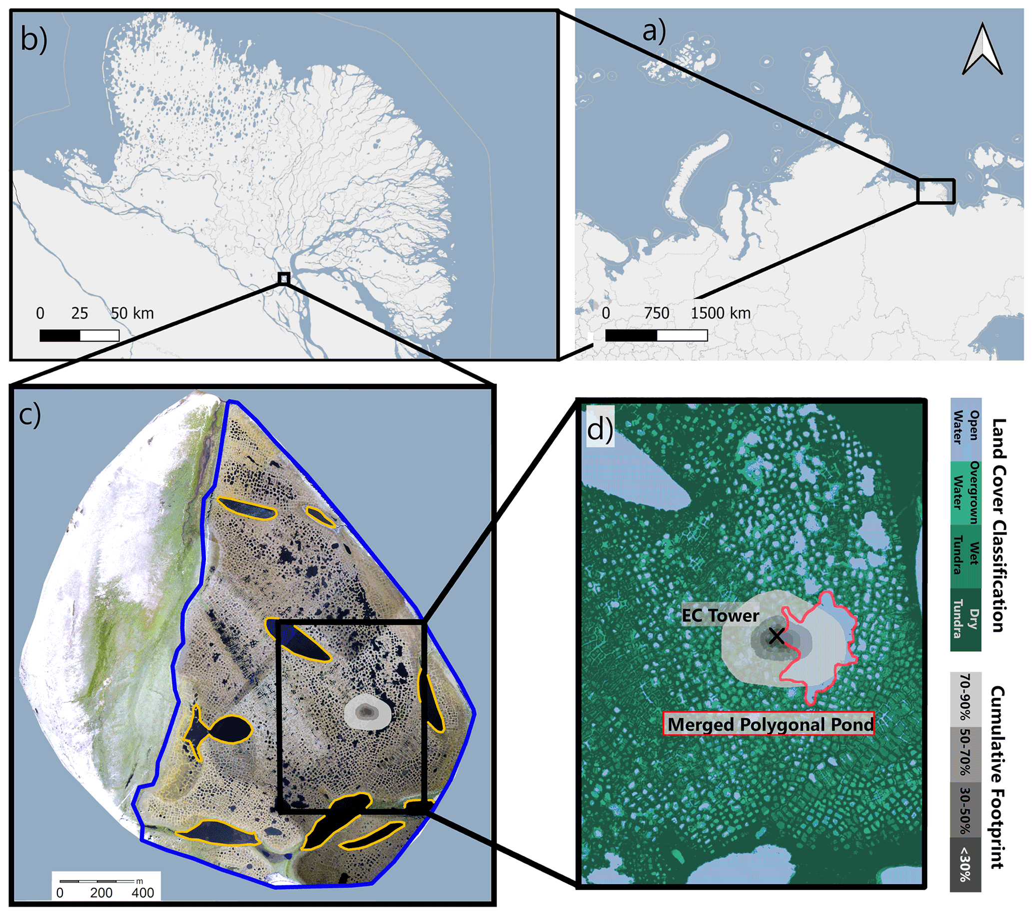
Figure 1The location of the study site in Russia is shown in (a), and the location of Samoylov Island within the Lena River delta is shown in (b). Samoylov Island is shown in (c); the surrounding Lena River appears in light blue. The outline of the river terrace land-cover classification (Sect. 2.4.1) is indicated by the blue line. We focus on the polygonal tundra; however, large lakes are excluded (circled in yellow). In (d), the land-cover classification is drawn in blue (open water) and green (dark green: dry tundra; medium green: wet tundra; light green: overgrown water) shades. The merged polygonal pond studied here is outlined in red. The location of the EC tower is marked by a black cross. The cumulative footprint (see Sect. 2.4.2) is shown in gray shades. Of the flux, 30 % likely originated from within the dark gray area, 50 % from within the medium dark gray area, 70 % from within the medium light gray area, and 90 % from within the light gray area. Map data from © OpenStreetMap contributors 2020, distributed under the Open Data Commons Open Database License (ODbL) v1.0 (a, b) and modified based on Boike et al. (2012) (c, d).
2.3 Data processing
We performed the raw data processing and computation of half-hourly fluxes for open-path and enclosed-path fluxes (CO2, CH4, and H2O) using EddyPro 7.0.6 (LI-COR, 2019). The convention of this software is that positive fluxes are fluxes from the surface to the atmosphere, while negative fluxes indicate a flux from the atmosphere downwards. Raw data screening included spike detection and removal according to Vickers and Mahrt (1997) (1 % maximum accepted spikes and a maximum of three consecutive outliers). Additionally, we applied statistical tests for raw data screening, including tests for amplitude resolution, skewness and kurtosis, discontinuities, angle of attack, and horizontal wind steadiness. All of these tests' parameters were set to EddyPro default values. We rotated the wind-speed axis to a zero-mean vertical wind speed using the “double rotation” method of Kaimal and Finnigan (1994). Further, we applied linear de-trending to the raw data following Gash and Culf (1996) before performing flux calculations. We compensated for time lags via automatic time lag optimization using a time lag assessment file from a previous EddyPro run. In this previous time lag assessment, the time lags for all gases were detected using covariance maximization (Fan et al., 1990), resulting in time lags between 0 and 0.4 s for CO2 and between −0.5 and +0.5 s for CH4. For H2O, the time lag was humidity-dependent and was calculated for 10 humidity classes. We compensated for air-density fluctuations due to thermal expansion and contraction and varying water-vapor concentrations, following Webb et al. (1980). This correction depends on accurate measurements of the latent and sensible heat flux and was applied to the open-path data of the LI-7700. For the LI-7700 in particular, the correction term can be larger than the flux itself, but the correction was derived from the underlying physical equations. Because we used well-calibrated instruments as well as EddyPro, which uses an up-to-date implementation of the correction, we were confident that the LI-7700 would provide accurate CH4 flux estimates. For enclosed-path data, we performed a sample-by-sample conversion into mixing ratios to account for air-density fluctuations (Ibrom et al., 2007b; Burba et al., 2012). Flux losses occurred in the low- and high-frequency spectral range due to different filtering effects. We compensated for flux losses in the low-frequency range in accordance with Moncrieff et al. (2004) and in the high-frequency range in accordance with Fratini et al. (2012). For the high-frequency range compensation method, a spectral assessment file was created using the method of Ibrom et al. (2007a). The spectral assessment resulted in cutoff frequencies of 3.05 and 1.67 Hz for CO2 and CH4, respectively. For H2O, we found a humidity-dependent cutoff frequency between 1.25 Hz (relative humidity, RH, of 5 %–45 %) and 0.21 Hz (RH 75 %–95 %). We performed a quality check on each half-hourly flux following the 0–1–2 system proposed by Mauder and Foken (2004). In this quality check, flux intervals with the lowest quality received the flag “2” and were excluded from further analysis.
2.4 Data analysis
2.4.1 Land-cover classification
The land-cover classification covers the Late Holocene river terrace of Samoylov Island (3.0 km2, area within the blue line in Fig. 1c). It is based on high-resolution near-infrared (NIR) orthomosaic aerial imagery obtained in the summer of 2008 (Boike et al., 2015b). We used a subset of the existing classification of Muster et al. (2012) as a training dataset to perform semi-supervised land-cover classification using the maximum likelihood algorithm in ArcMap Version 10.8 (Esri Inc., USA). We then applied the ArcMap majority filter tool to the new classification. The land-cover classification has a resolution of 0.17 m × 0.17 m,. It is projected onto WGS 84 UTM Zone 52N, and the land-cover classes include open water (15.7 %), overgrown water (7.0 %), dry tundra (65.1 %), and wet tundra (12.1 %), as defined by Muster et al. (2012). We summarize the classes overgrown water, dry tundra, and wet tundra in the land-cover type of semi-terrestrial tundra. The river terrace consists of this semi-terrestrial tundra, large lakes, and thermokarst ponds. Since small ponds are an integral part of the polygonal tundra, we use the term “polygonal tundra” to refer to the area of the river terrace covered by semi-terrestrial tundra and by thermokarst ponds.
2.4.2 Footprint model
In deploying an EC measurement tower, the tower's location and sensor height are crucial parameters. A lower measurement height results in a smaller footprint. The tower's footprint describes the source area of the flux within the surrounding landscape. As we installed sensors at a height of 2.25 m next to the merged polygonal pond, we expected to observe substantial flux signals from the adjacent water body as well as from the surrounding semi-terrestrial tundra. Each land-cover type's contribution to the flux signal depended on the wind direction and turbulence characteristics. We implemented the analytical footprint model proposed by Kormann and Meixner (2001) in MATLAB (2019). We combined the footprint model with land-cover classification data described in Sect. 2.4.1 to estimate the contribution of each land-cover type to each half-hourly flux (from now on referred to as the weighted footprint fraction). The model accounted for the stratification of the atmospheric boundary layer and required a height-independent crosswind distribution and horizontal homogeneity of the surface. The input data required stationarity of atmospheric conditions during the flux intervals of 30 min.
We derived the vertical power-law profiles for the eddy diffusivity and the wind speed for each 30 min flux depending on the atmospheric stratification (see Eq. 6 in Kormann and Meixner, 2001). We used an analytical approach to find the closest Monin–Obukhov (M–O) similarity profile (see Eq. 36 in Kormann and Meixner, 2001). Next, we calculated a two-dimensional probability density function of the source area for each flux (from Eqs. 9 and 21 in Kormann and Meixner, 2001). We combined each probability density function with the land-cover classification of Samoylov Island's river terrace with its four land-cover types (see Sect. 2.4.1). The resolution of the footprint model was set to the land-cover classification resolution of 0.17 m × 0.17 m. Hence, we were able to estimate how much a given grid cell contributed to each 30 min flux. We also knew each grid cell's dominant land-cover type from the land-cover classification. We combined both pieces of information for each grid cell and calculated the sum of the fraction fluxes within the source area for each of the four land-cover types (dry tundra, wet tundra, overgrown water, and open water) and determined the contribution of each land-cover type with respect to each 30 min flux (adry tundra, awet tundra, aovergrown water, and aopen water). We refer to this contribution of each land-cover type as the weighted footprint fraction.
We also summed all 30 min two-dimensional probability density functions over the entire deployment time. This sum is referred to as the cumulative footprint (gray-shaded area in Fig. 1c–d).
2.4.3 Gap-filling the CO2 flux
To gap fill the net ecosystem exchange (NEE) fluxes of CO2, we used the bulk-NEE model proposed by Runkle et al. (2013). The model is specifically designed to model NEE in Arctic regions: it takes impacts of the polar day into account by allowing both respiration and photosynthesis to occur simultaneously throughout the day. The bulk-NEE model uses the sum of total ecosystem respiration (TER) and gross primary production (GPP) to describe NEE, our target variable:
where TER and GPP are in units of µmol m−2 s−1. TER is approximated as an exponential function of air temperature Tair:
where Tref=15 ∘C and γ=10 ∘C are constant, independent parameters. Rbase (µmol m−2 s−1) describes the basal respiration at the reference temperature Tref, and Q10 (dimensionless) describes the sensitivity of ecosystem respiration to air temperature changes.
GPP is described as a rectangular hyperbolic function of PAR (µmol m−2 s−1):
where α (µmol µmol−1) is the initial canopy quantum use efficiency (slope of the fitted curve at PAR =0) and Pmax (µmol m−2 s−1) is the maximum canopy photosynthetic potential for PAR →∞.
The parameters Rbase, Q10, Pmax, and α were fitted simultaneously. To account for seasonal changes in plant physiology, we fitted the parameters for 5 d running windows as proposed in Holl et al. (2019).
We split the datasets into training (70 %) and validation (30 %) datasets to test model performance. We implemented the bulk-NEE model in MATLAB 2019b (MATLAB, 2019) using the fit function with the NonLinearLeastSquares fitting method. We used the coeffvalues function to estimate the four parameters (Rbase, Q10, Pmax, and α) and the confint function to estimate their 95 % confidence bounds. All partitioned fluxes were converted into CO2–C fluxes in units of g m−2 d−1 before data analysis.
2.4.4 Separating CO2 fluxes from semi-terrestrial tundra and water bodies
We wanted to extract fluxes from thermokarst ponds and semi-terrestrial tundra to analyze the influence of thermokarst ponds on the carbon balance of a polygonal tundra landscape. However, due to the strong heterogeneity of the landscape and the relatively small size of the merged polygonal pond compared to the EC footprint, we measured a mixed signal from all wind directions. In other words, each flux that was measured with the EC method contained information from different land-cover types. We divided the footprint into two classes – semi-terrestrial tundra and thermokarst ponds – to assess the impact of thermokarst ponds on the carbon balance.
Similar approaches of analyzing heterogeneous eddy covariance fluxes in Arctic environments have been conducted for CO2 and CH4 (e.g., Rößger et al., 2019a, b; Tuovinen et al., 2019). Rößger et al. (2019a, b) extracted CO2 and CH4 fluxes from two different land-cover classes on a floodplain, while Tuovinen et al. (2019) separated CH4 fluxes from nine individual land-cover classes, including water, and combined them into four source classes (with no separate class for water). All three studies differentiate between fluxes from different vegetation types. Our method is dedicated to distinguishing between fluxes from semi-terrestrial tundra and water bodies.
To estimate CO2 fluxes from the merged polygonal pond (Fpond), we first fitted the bulk-NEE model to training data, excluding fluxes from the direction of the merged polygonal pond (30∘ < WD < 150∘, where WD denotes wind direction). We obtained a dataset consisting of information about as much semi-terrestrial tundra as possible. We performed this step since we expected little to no photosynthetic activity in the open-water part of the merged polygonal pond. This gap-filled CO2 flux (hereinafter Fmodeled,mix) represents the polygonal tundra surrounding the EC tower, meaning the flux is dominated by semi-terrestrial tundra, but also includes polygonal ponds from the wind directions of north, west, and south. In the model input, we excluded 30 min CO2 fluxes with an absolute value of more than 4 g m−2 d−1. In 38 windows of 5 d duration, we found an R2 above 0.9 between the model output and the validation set. In 18 cases, we obtained an R2 between 0.8–0.9; in six instances, we obtained an R2 below 0.7. The final RMSE between the model input and the gap-filled NEE had a value of 0.29 g m−2 d−1.
We assumed that the total observed flux was a linear combination of the fluxes from the land-cover types weighted by their respective contribution to the footprint. Thus, we postulated that the observed CO2 flux (Fobs,mix, not gap-filled) was the sum of the individual land-cover type fluxes (Fmodeled,mix and the merged polygonal pond Fpond) each multiplied with their weighted footprint fraction (amix and apond), with aopen water=apond, , and asum being the sum over all land-cover classes:
To improve data quality, we excluded 30 min fluxes of Fpond when apond<50 %. Then, we used the median of Fpond for further calculations, and we assumed that all thermokarst ponds in the EC footprint emitted the same amount of CO2.
As mentioned above, the observed CO2 flux from the wind directions of north, west, and south (Fobs,mix) was influenced by polygonal ponds to a small degree. Since our aim was to assess the impact of thermokarst ponds (both polygonal ponds and merged polygonal ponds) on NEE, we needed to eliminate the influence of polygonal ponds from our NEE estimate. To extract uncontaminated CO2 flux data from the semi-terrestrial tundra (Fmodeled,tundra), we subtracted the previously estimated pond CO2 flux Fpond from the observed CO2 flux Fobs,mix:
We then used this estimated CO2 flux from the semi-terrestrial tundra Fmodeled,tundra as the regressand variable for the bulk-NEE model to obtain a gap-filled dataset regarding CO2 flux from the semi-terrestrial tundra. This gap-filling modeling of CO2–C flux had an RMSE of 0.31 g m−2 d−1.
To evaluate the impact of thermokarst ponds on landscape CO2 flux, we estimated a polygonal tundra landscape–CO2 flux from the Late Holocene river terrace of Samoylov Island (Flandscape) by combining thermokarst ponds and semi-terrestrial tundra linearly:
where Fpond describes the CO2 emissions from the open-water areas of thermokarst ponds (Eq. 4), Fmodeled,tundra describes the modeled CO2 flux from the semi-terrestrial tundra (Eq. 5), Apond=0.07 is the fraction of the river terrace area of Samoylov Island that is covered by thermokarst ponds (from the land-cover classification; see Sect. 2.4.1), and is the fraction of the entire river terrace area that consists of other land-cover types. We did not account for larger or deeper lakes in this upscaling approach as we expected different greenhouse gas emission dynamics from these lakes and there were no lakes in our footprint and therefore within our observation range. Thus, we scaled the above numbers to , which results in Apond=0.076 and Atundra=0.924.
2.4.5 CH4 flux partitioning
The data show that the CH4 emissions from the heterogeneous landscape around the tower were less spatially uniform than the CO2 emissions. Therefore, we could not use a gap-filling model for CH4 that was similar to the bulk model we used for CO2, so we investigated CH4 emissions in a different way. Based on preliminary results from our analysis and the aerial image of the study site, we focused on four wind sectors instead of extracting the fluxes from the land-cover types:
-
Tundra. At least half of the footprint consisted of dry tundra, and the wind direction was larger than 170∘.
-
Shore 50∘ (denoted shore). Less than 40 % of the footprint consisted of dry tundra, and water comprised at least 30 % of the footprint. The wind direction range was 30∘ < WD < 65∘.
-
Pond. At least half of the footprint consisted of open water, and the wind direction range was 65∘ < WD < 110∘.
-
Shore 120∘ (denoted shore). Less than 40 % of the footprint consisted of dry tundra, and water comprised at least 30 % of the footprint. The wind direction range was 110∘ < WD < 130∘.
2.4.6 CH4 permutation test
To evaluate whether the differences in flux medians between the four wind sectors were significant, we applied a permutation test (Edgington and Onghena, 2007). In this test, we randomly assigned each 30 min flux to one of two groups and calculated both groups' medians and the differences between the group's medians. We conducted six tests in total, using all possible combinations of pairs with the four wind sectors. After repeating this step 10 000 times, we plotted the resulting differences in medians in a histogram and performed a one-sample t test to evaluate whether the observed difference in medians differed significantly (p<0.01) from the randomly generated differences.
3.1 Meteorological conditions
During the measurement period between 11 July and 10 September 2019, half-hourly air temperatures range from −0.5 to 27.6 ∘C with a mean temperature of 8.7 ∘C (Fig. A2a). The maximum wind speed measured at the EC tower at a height of 2.25 m is 8.9 m s−1 (Fig. A2b). PAR reaches values of up to 1419 µmol m−2 s−1 with decreasing maximum values during the measurement period (Fig. A2c). Throughout the measurement period, there are 28 cloudy days, determined by identifying days with low PAR values (maximum values below ∼ 500 µmol m−2 s−1).

Figure 2Polar plot of observed 30 min CO2–C fluxes with respect to the wind direction. Negative values (inside of the dashed black line) represent CO2 uptake, while positive values (outside of the dashed black line) represent CO2 emissions. The values −4, −2, 0, and 2 indicate the magnitude of the CO2–C flux in g m−2 d−1. The color of each point on the plot represents the percentage the point comprises of the total open-water weighted footprint fraction in each 30 min flux. The red boxes indicate the mean CO2 flux of 5∘ wind direction intervals during the 2-month observation period (red lines indicate the first standard deviation).
3.2 CO2 fluxes
When inspecting the relation between observed CO2 fluxes and wind direction (Fig. 2), we find that CO2 fluxes exhibit high temporal variability between positive and negative CO2 fluxes from most wind directions. In the wind sector between 60–120∘, the flux source area is dominated by the merged polygonal pond. The CO2–C fluxes from this pond sector show smaller absolute variability ( g m−2 d−1, median) than the fluxes from all other wind directions ( g m−2 d−1, median). Additionally, we observe a lower respiration rate from the merged polygonal pond than from the semi-terrestrial tundra. Figure 3 shows the observed nighttime CO2 fluxes plotted against the respective weighted footprint fraction of open water. We define nighttime as having PAR < 20 µmol m−2 s−1; we expect that there would only be respiration and no photosynthesis during the nighttime. We find that the fluxes decrease as the pond area contribution increases. Thus, the strength of CO2 respiration shows a dependence on the contribution of open water. We also find that low air temperatures are mostly associated with low respiration rates.
Another aspect of CO2 flux variability stems from the diurnal cycle. We compare the diurnal cycle of the CO2 fluxes from the merged polygonal pond (estimated in accordance with Eq. 4) and the semi-terrestrial tundra (Eq. 5, Fig. 4). The results show a less pronounced diurnal CO2 cycle from the direction of the merged polygonal pond (blue) compared to the diurnal CO2 cycle from the semi-terrestrial tundra (green). We combine all data from the merged polygonal pond (Fpond in Eq. 4), which results in a CO2–C flux of g m−2 d−1 (median).
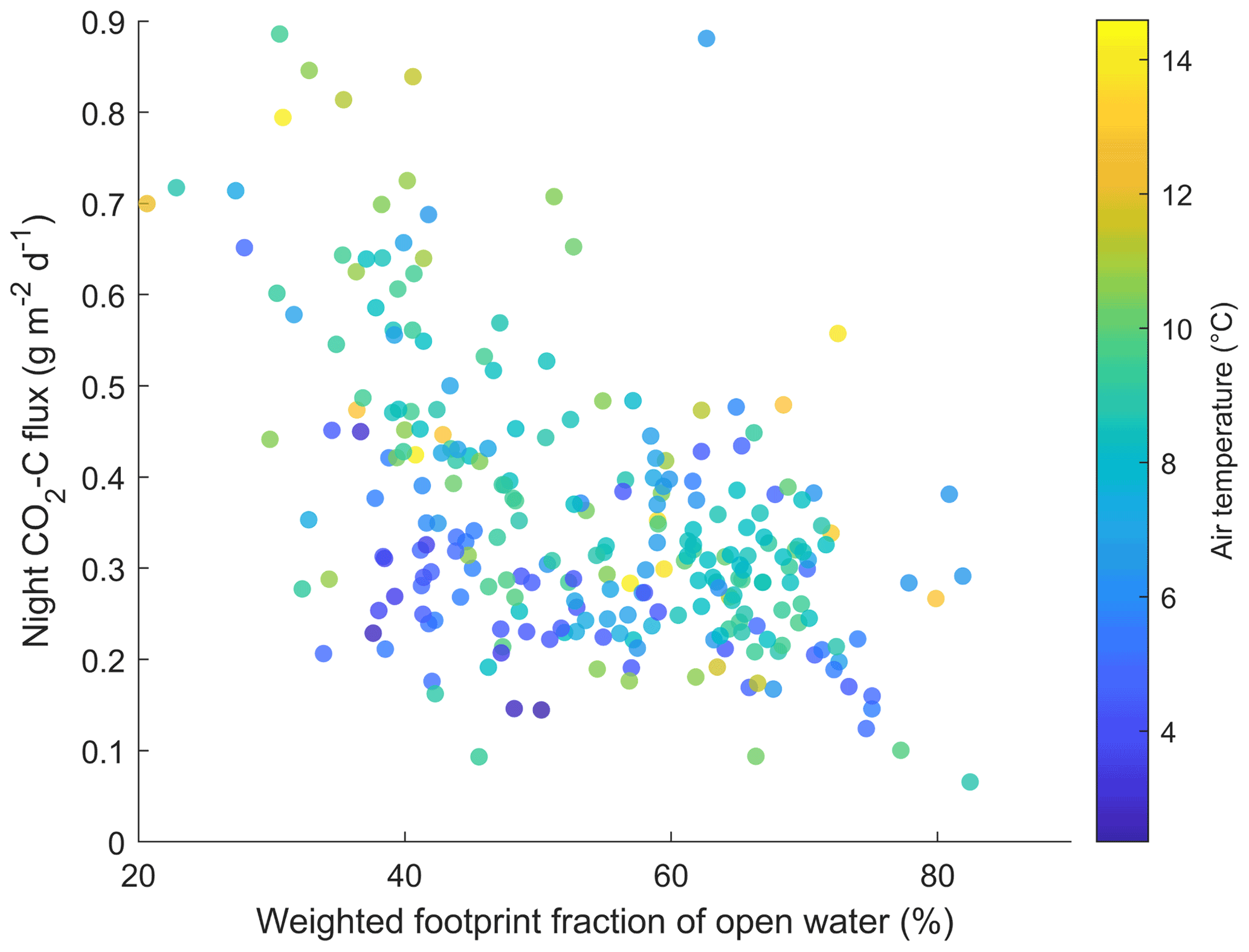
Figure 3Scatterplot of observed CO2 fluxes against the weighted footprint fraction of open water during each 30 min flux. The air temperature is represented through color. Only fluxes observed in the nighttime (PAR < 20 µmol m−2 s−1) are shown.
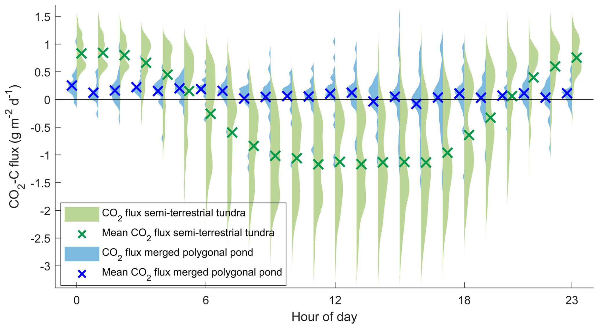
Figure 4Diurnal cycle of modeled CO2–C based on observations flux from the merged polygonal pond (blue, Eq. 4) and the semi-terrestrial tundra (green, Eq. 5) as violin plots for each half-hour flux. Blue and green crosses mark the mean CO2–C flux during each half-hour flux. A violin plot shows the distribution of measurements along the y axis – the width of the curves indicates how frequently a certain y value occurred.
3.3 CH4 fluxes
We plot the observed CH4 fluxes against wind direction (Fig. 5). The results show that the CH4 emissions peak at , where fluxes from one shoreline of the merged polygonal pond contribute to the observed flux (Fig. 1d, from now on shore). We do not observe a similar peak of CH4 emissions in the direction of the second shoreline towards (shore). These peaks did not correlate with a specifically large contribution of one of the land-cover classes to the footprint.
To further investigate the peak at shore, we compare the CH4 emissions from the different wind sectors (shore, shore, pond, and tundra; Sect. 2.4.5). We find the following fluxes from the wind sectors: (shore), (shore), (pond), and mg m−2 d−1 (tundra, median). Fluxes from shore have a higher median than fluxes from the other three wind sectors (Fig. 6).
We investigated the impact of wind speed and air temperature on the CH4 fluxes by excluding flux intervals with high wind speed (greater than 5 m s−1) and high air temperature (warmer than 12 ∘C). The randomization test (Sect. 2.4.6) provided evidence of a significant difference between CH4 emissions from shore and the other three wind sector classes at low wind speeds (top row in Fig. A4) and no significant difference between the CH4 emissions from the classes pond–tundra and shore–tundra. The difference between the classes pond and shore is significant; however, it is much smaller than the previously described differences (see central graph in Fig. A4). Note that the CH4 emissions from pond and tundra have a similar magnitude under moderate wind-speed conditions. The results are very similar for moderate temperatures: we find evidence of a significant difference between the CH4 emissions from shore and the CH4 emissions from the other three wind sector classes (top row in Fig. A5). The differences in medians between the pond and shore and between the pond and tundra are significant. However, this difference is much smaller (second row in Fig. A5). In summary, neither high wind speed nor high temperatures act as a driver for the high CH4 emissions from shore. In contrast, the peak at 180–190∘ can be explained reasonably well using air temperature and friction velocity in multiple linear regression (R2=0.44). Using the same predictors results in an R2 of 0.20 for the peak at shore.
The ratio of CO2–C to CH4–C emissions at night (PAR < 20 µmol m−2 s−1) has a value of CH4 CO for fluxes with an open-water weighted footprint fraction of more than 60 %, whereas the ratio amounts to CH4 CO (median) for fluxes with an open-water weighted footprint fraction of less than 20 %.
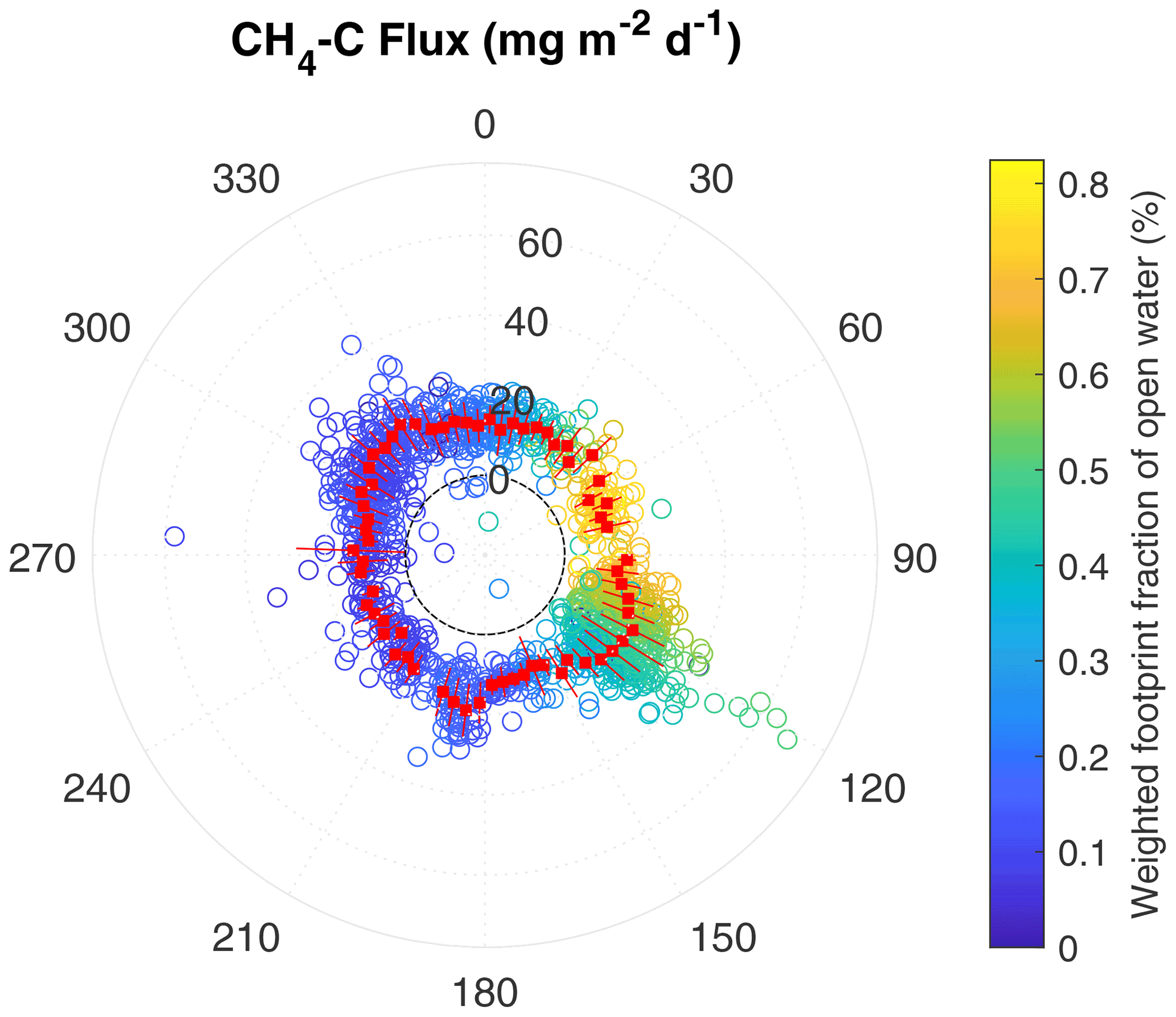
Figure 5Polar plot of 30 min observed CH4–C flux with respect to the wind direction at the EC tower. Positive values outside the dashed black line represent CH4 emissions, while values inside the line represent CH4 uptake during one half-hour period. The values 0, 20, 40, and 60 indicate the magnitude of the CH4–C flux in mg m−2 d−1. The color of each point on the plot represents the percentage the point comprises of the total open-water weighted footprint fraction in each 30 min flux. The red boxes indicate the mean CH4 flux of 5∘ wind direction intervals during the 2-month observation period (red lines indicate the first standard deviation).
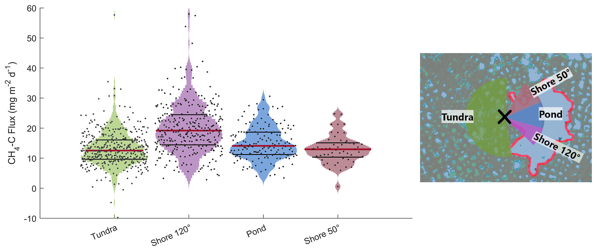
Figure 6Violin plots of observed CH4 emissions at the EC tower separated into four different wind sector classes. A violin plot shows the distribution of measurements along the y axis – the width of the shapes indicates how frequently a certain y value occurred. Medians of CH4 emission distributions are shown as red lines, and 75th and 25th percentile are shown as black lines. On the right, the wind sectors with the eddy covariance tower in the center (black cross) are shown.
3.4 Upscaled CO2 flux
We use the estimated open-water CO2 flux from the merged polygonal pond and the modeled CO2 flux from the semi-terrestrial tundra to linearly upscale the CO2 flux for the polygonal tundra of Samoylov Island (excluding larger lakes, the method described in Sect. 2.4.4). As we have not obtained estimates for the CH4 fluxes from tundra and pond land-cover types, we only upscale CO2.
We estimate that when one includes the CO2 flux from thermokarst ponds, the river terrace landscape's CO2 uptake is ∼ 11 % lower than the uptake of semi-terrestrial tundra without ponds. The modeled CO2–C flux from the semi-terrestrial tundra (without consideration of thermokarst pond fluxes) accumulated to −16.29 ± 0.43 g m−2 during the observation period (60.5 d). If separated into months, the modeled CO2–C flux from the semi-terrestrial tundra amounts to −15.01 ± 0.26, −3.56 ± 0.33, and +2.35 ± 0.11 g m−2 in July (19.8 d), August (31 d), and September (9.7 d), respectively. When one includes the CO2 flux from the merged polygonal pond to represent all thermokarst ponds on Samoylov Island, the resulting estimate of the landscape CO2 flux amounts to −14.47 ± 0.40 g m−2 (60.5 d), with monthly fluxes of −13.75 ± 0.24, −2.99 ± 0.31, and +2.27 ± 0.10 g m−2 in July (19.8 d), August (31 d), and September (9.7 d), respectively. Thus, the results show that thermokarst ponds have the largest impact on the landscape's CO2 flux in August. In September, accounting for thermokarst ponds leads to a 3.5 % lower estimate of landscape CO2 emissions.
4.1 CO2 flux
Only a limited number of EC CO2 flux studies from permafrost-affected ponds and lakes are available (studies with “EC” in Table 1). Estimates of open-water EC CO2–C flux range from 0.059 (Jammet et al., 2017) to 0.11 (Eugster et al., 2003) to 0.22 g m−2 d−1 (Jonsson et al., 2008). Our estimate of g m−2 d−1 is, therefore, well within the range of open-water CO2–C fluxes observed with the EC method. Other studies using different methods report a wider range of open-water CO2 fluxes in Arctic regions. These fluxes range from a minor CO2–C uptake (−0.14 g m−2 d−1; Bouchard et al., 2015) to substantial emissions of CO2–C (up to 2.2 g m−2 d−1; Abnizova et al., 2012). A modeling study involving multiple lakes in northeast European Russia found that they produce almost zero emissions (0.028 g m−2 d−1; Treat et al., 2018).
Abnizova et al. (2012)Jammet et al. (2017)Jonsson et al. (2008)Eugster et al. (2003)Jansen et al. (2019)Bouchard et al. (2015)Sepulveda-Jauregui et al. (2015)Treat et al. (2018)Sieczko et al. (2020)Ducharme-Riel et al. (2015)Repo et al. (2007)Lundin et al. (2013)Kling et al. (1992)Table 1Daily mean water–atmosphere CO2 and CH4 fluxes from different study sites. TBL is the abbreviation for thin boundary layer model, EC for eddy covariance, CH for chamber measurement, MOD for modelled fluxes, STO for storage fluxes, and NEW for the method used in this study. All fluxes are given ± standard deviation, except fluxes from this study are given as median.

Strikingly, our estimates of open-water CO2 emissions are approximately 12–18 times smaller than those that have been previously reported for open-water CO2 emissions at the same study site (Abnizova et al., 2012). One reason for the divergent results might be the different methods used. In Abnizova et al. (2012), the thin boundary layer (TBL) model, following Liss and Slater (1974), was applied to estimate CO2 emissions from CO2 concentrations. However, one other study found good agreement between the EC method and the TBL one (Eugster et al., 2003). In addition, in contrast to the larger merged polygonal pond we focus on, Abnizova et al. (2012) measured two polygonal ponds (they took 46 water samples in August and September 2008). These two ponds might have had exceptionally high CO2 concentrations and might not be representative of polygonal ponds in our study area. If the polygonal ponds in the footprint of our EC measurements emitted CO2 in the quantities suggested by Abnizova et al. (2012), we would expect to see their signal more clearly in our measurements.
Our approach of combining a footprint model with land-cover classification to extract fluxes from different land-cover classes allows us to determine the thermokarst pond CO2 flux. We report an uncertainty range with respect to the thermokarst pond CO2 flux; however, identifying the full uncertainty in this flux is not possible using this approach due to the footprint analysis' unknown degree of uncertainty. Still, the results with respect to the thermokarst pond CO2 flux are plausible and on the expected order of magnitude for two reasons. First, reduced diurnal variability is observed when the merged polygonal pond influences the flux signal (Fig. 4). This reduction indicates that the respiration rate from the merged polygonal pond is lower than the respiration rate from the semi-terrestrial tundra, where ample oxygen is available in the upper soil layer. Additionally, since the thermokarst ponds have a lower vegetation density than the tundra, there is less photosynthesis. Second, when focusing on nighttime fluxes, when only respiration occurs (i.e., no carbon is taken up), there is a decrease in CO2 emissions with an increasing weighted footprint fraction of open water (Fig. 3); this also indicates that there is reduced decomposition in the merged polygonal pond. Overall, based on the data, the finding that thermokarst ponds have lower CO2 emissions than the semi-terrestrial tundra is reasonable.
4.2 CH4 flux
We observe large differences in CH4 emissions from the four wind sectors. CH4 emissions from shore are significantly higher than from shore, pond, and tundra (Sect. 3.3). Notably, we tested the dependence of these higher fluxes on wind speed and air temperature. We expect high wind speeds to enhance turbulent mixing of the water column and diffusive CH4 outgassing at the water–atmosphere interface. High wind speeds are also associated with pressure pumping, which potentially fosters the ebullition of CH4. On the other hand, peak temperatures can lead to peak CH4 production and emissions due to enhanced biological activity. However, the high emissions from shore do not coincide with either of two key meteorological conditions, high wind speeds and high temperatures, which would especially favor high emissions. Thus, the difference in methane flux dynamics between shore and shore is astounding since the shorelines share many other characteristics.
Both shorelines extend radially (in a fairly straight line) from the EC tower (Fig. 1), thus contributing similarly to the EC flux. The underwater topography does not vary significantly between the two shorelines. Meters away from the shore, both shorelines have a water depth of a few centimeters and a few decimeters (see data from Boike et al., 2015a). As previously described in Sect. 2.1, both shorelines are dominated by Carex aquatilis, and from visual inspection, we could not identify differences in shoot density. We, therefore, assume that the characteristics of the emergent vegetation do not play a major role in explaining the differences between the CH4 emissions from shore and shore. We also examine the evolution of the shorelines at the merged polygonal pond to check whether erosion along the shoreline could cause the high CH4 emissions. We compare an image from 1965 (Earth Resources Observation and Science (EROS) Center, 2018) with the current (2019) shoreline, yet we cannot identify signs of recent erosion. Furthermore, high-resolution aerial images of this pond from 2008 (Boike et al., 2015b, resolution > 0.33 m) and 2015 (Boike et al., 2015c, resolution > 0.33 m) show no signs of erosion. We therefore assume that past erosion is unlikely is unlikely to have been a factor that caused the high levels of CH4 emissions we observed in 2019.
Local ebullition of the merged polygonal pond could lead to high CH4 emissions from shore. We applied the method proposed by Iwata et al. (2018) to check for signs of ebullition events. This method uses the 20 Hz raw CH4 concentration data to detect short-term peaks in CH4 that originate from ebullition events. However, we cannot detect ebullition events in the 20 Hz raw data.
In summary, meteorological conditions (wind speed and temperature), characteristics of emergent vegetation, coastal erosion, and intense ebullition events are unlikely to be the main driving factors of the increased CH4 emissions we observed. Another possible driver of higher CH4 emissions from shore is a small but steady seep ebullition hot spot close to this shoreline (such as ebullition class kotenok in Walter et al., 2006). Seep ebullition hot spots have been reported to occur heterogeneously in clusters in Alaskan lakes (Walter Anthony and Anthony, 2013). Unfortunately, seep ebullition has not previously been reported in water bodies in our study area, so we did not include measurements targeting this process in our measurement campaign. In future studies, visual inspection of trapped CH4 bubbles in the ice column during wintertime, as proposed by Vonk et al. (2015), could reveal more information about the cause of the higher CH4 emissions from shore, as could funnel or chamber measurements with high spatial coverage.
The results show that the merged polygonal pond emits a similar magnitude of CH4 to the polygonal tundra surface under similar meteorological conditions and when excluding the high emissions from shore. However, substrate availability and temperature dynamics differ substantially. Additionally, in dense soils, methane diffuses slowly enough through soil layers containing oxygen for the methane to be oxidized before reaching the surface. In contrast, methane emitted in ponds can reach the surface quickly through ebullition or plant-mediated transport in addition to diffusion. Therefore, we expect to see larger differences between the CH4 emissions from the merged polygonal pond and the polygonal tundra, more akin to the differences that have been detected in a subarctic lake and fen by Jammet et al. (2017). However, we see no significant difference in the CH4 emissions from the open-water areas of the merged polygonal pond and the polygonal tundra surface (Figs. 6 and A4).
Since many other thermokarst ponds in our study area are smaller than the merged polygonal pond (making them unsuitable to study using the EC method) and since smaller ponds tend to be greater emitters of methane (Holgerson and Raymond, 2016; Wik et al., 2016), our measurements might provide a lower limit of overall thermokarst pond CH4 emissions.
We estimate a CH4–C flux of mg m−2 d−1 () from the merged polygonal pond and – mg m−2 d−1 from the shores of this pond. This is higher than the fluxes measured by Jammet et al. (2017) from a subarctic lake (Table 1). The authors report a mean annual CH4–C flux of 13.42 ± 1.64 mg m−2 d−1 and a mean ice-free-season CH4–C flux of 7.58 ± 0.69 mg m−2 d−1. A study focusing on 32 non-Yedoma thermokarst lakes in Alaska found CH4–C emissions similar to our results (16.80 ± 8.61 mg m−2 d−1; Sepulveda-Jauregui et al., 2015). Also, a synthesis of 149 thermokarst water bodies north of N reports CH4–C emissions on the same order of magnitude (27.57 ± 14.77 mg m−2 d−1; Wik et al., 2016). However, other recent studies have reported considerably lower CH4–C emissions of 2.95 ± 0.75 mg m−2 d−1 in northern Sweden (Sieczko et al., 2020), and, in contrast, a study found CH4–C emissions of up to 6432 mg m−2 d−1 in northeast Canada (Bouchard et al., 2015). The wide range of water-body methane emissions militates in favor of caution when generalizing our results, even for Samoylov Island, especially since the emissions within the merged polygonal pond have been shown to be heterogeneous. Instead, after finding a hot spot in CH4 emissions at the pond shore, we would like to highlight that the gathering of additional measurements – for example employing funnel traps or counting bubbles in ice – will help to better constrain thermokarst pond CH4 dynamics in their full complexity. Nevertheless, our measurements provide a robust lower limit of thermokarst pond CH4 emissions.
4.3 Upscaling the CO2 flux
We upscale the CO2 emissions for the river terrace on Samoylov, an area for which we have access to high-resolution land-cover classification. We find that we overestimate the carbon dioxide uptake of the polygonal tundra by 11 % when we do not account for the thermokarst ponds' CO2 emissions. A similar approach by Abnizova et al. (2012) found a potential increase of 35 %–62 % in the estimate of CO2 emissions from the Lena River delta when including small ponds and lakes in the landscape CO2 emission calculation. If we were to follow the upscaling approach by Abnizova et al. (2012) and consider overgrown water as part of the thermokarst ponds, the estimate of the landscape CO2 uptake would decrease by 19 %. Kuhn et al. (2018) also found water bodies in Arctic regions to be an important source of carbon, which could outbalance the carbon dioxide uptake of the semi-terrestrial tundra in a future climate. In summary, our results demonstrate that open-water CO2 emissions can substantially influence the summer carbon balance of the polygonal tundra. With respect to the night time emissions, we find that per gram CO2–C thermokarst ponds emit 0.06 g CH4–C whereas the semi-terrestrial tundra only emits 0.02 g CH4–C. This finding underlines again that, especially when considering thermokarst ponds, CH4 emissions are of significant interest. Even though mean CH4 emissions from the semi-terrestrial tundra and open water are of similar magnitude, we expect that the impact of thermokarst ponds on the carbon balance would be even greater when accounting for CH4 due to locally high emissions.
Our results suggest that future studies that aim to capture a representative landscape flux should pay extra attention to the water bodies in their footprint. The CO2 flux from thermokarst ponds has the opposite sign (CO2 emissions) to the semi-terrestrial tundra (CO2 uptake) during the observation period. Consequently, thermokarst ponds should cover about as much area in the measurement as they do in the landscape area of interest. In this way, the chances of capturing CH4 hot spots, which can be investigated more closely, are also greater.
We find that thermokarst ponds are a carbon source. At the same time, the surrounding semi-terrestrial tundra in our study area acts as a carbon sink during the summer period (July–September), which is in agreement with prior studies (Abnizova et al., 2012; Jammet et al., 2017), despite us observing much lower open-water CO2 fluxes compared to previous work at the same study site (Abnizova et al., 2012). Using our approach to disentangle the EC fluxes from different land-cover classes, we posit that during the measurement period, we would overestimate the carbon dioxide uptake of the polygonal tundra by 11 % if thermokarst ponds were not accounted for. We expect lakes to have a similar effect on the carbon budget, though a smaller one, since lakes (a) cover a similar amount of surface area as the thermokarst ponds in our study site (Abnizova et al., 2012; Muster et al., 2012) and (b) are weaker emitters of greenhouse gases than ponds (Holgerson and Raymond, 2016; Wik et al., 2016).
In contrast to CO2 emissions, which are spatially more homogeneous, small-scale heterogeneity in CH4 emissions makes it difficult to find drivers of CH4 emissions. We cannot pinpoint the drivers behind the high emissions along parts of the coastline, which we surmise were potentially caused by seep ebullition. Thus, we cannot estimate the impact of this heterogeneity on the landscape scale and, therefore, refrain from upscaling CH4 emissions. Additionally, the open-water fluxes presented in this paper originate from a single merged polygonal pond since the other polygonal ponds surrounding the EC tower are too small to extract their fluxes using the footprint method applied here. Thus, we do not account for the spatial variability in CH4 emissions between thermokarst ponds, which can be substantial (Rehder et al., 2021; Wik et al., 2016). However, we note that open-water fluxes were of a similar magnitude to the polygonal tundra fluxes. Consequently, the main impact that thermokarst ponds have on the landscape CH4 budget might occur through plant-mediated transport and local ebullition.
While being ill-suited for the study of smaller ponds, we underline that the EC method is appropriate for observing greenhouse gas fluxes from thermokarst ponds as small as 0.024 km2. The EC method has a higher temporal resolution than the TBL method. It does not disturb exchange processes like the chamber flux method, which eliminates the wind at the water surface. Especially when combining an EC footprint with land-cover classification, one can distinguish between the contribution of different land-cover classes effectively and also study the fluxes from thermokarst ponds.
We conclude that thermokarst ponds contribute significantly to the landscape carbon budget. Changes in Arctic hydrology and the concomitant changes in the water-body distribution in permafrost landscapes may cause these landscapes to change from being overall carbon sinks to overall carbon sources.
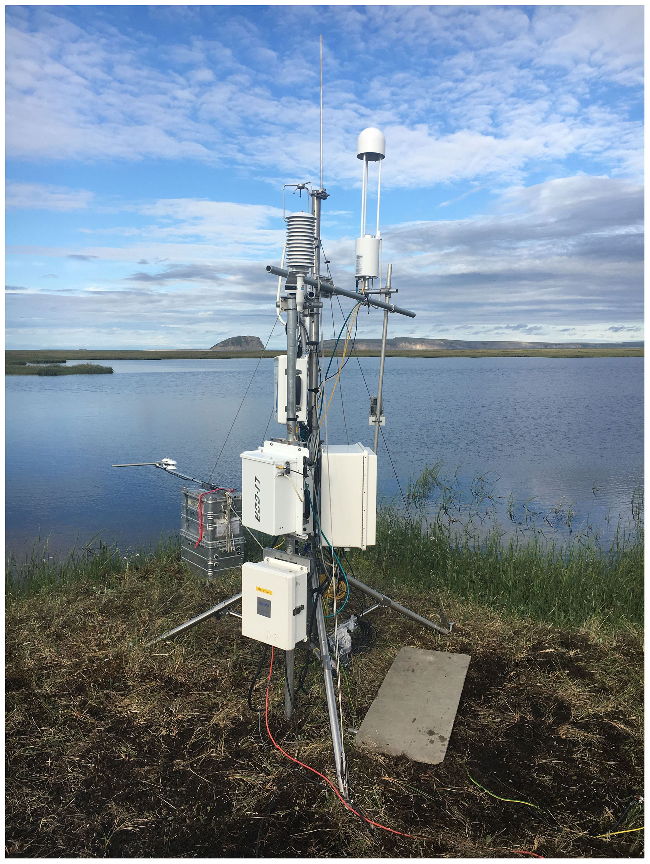
Figure A1Picture of the eddy covariance tower with the merged polygonal pond in the background. Picture taken on 11 July 2019 by Zoé Rehder.
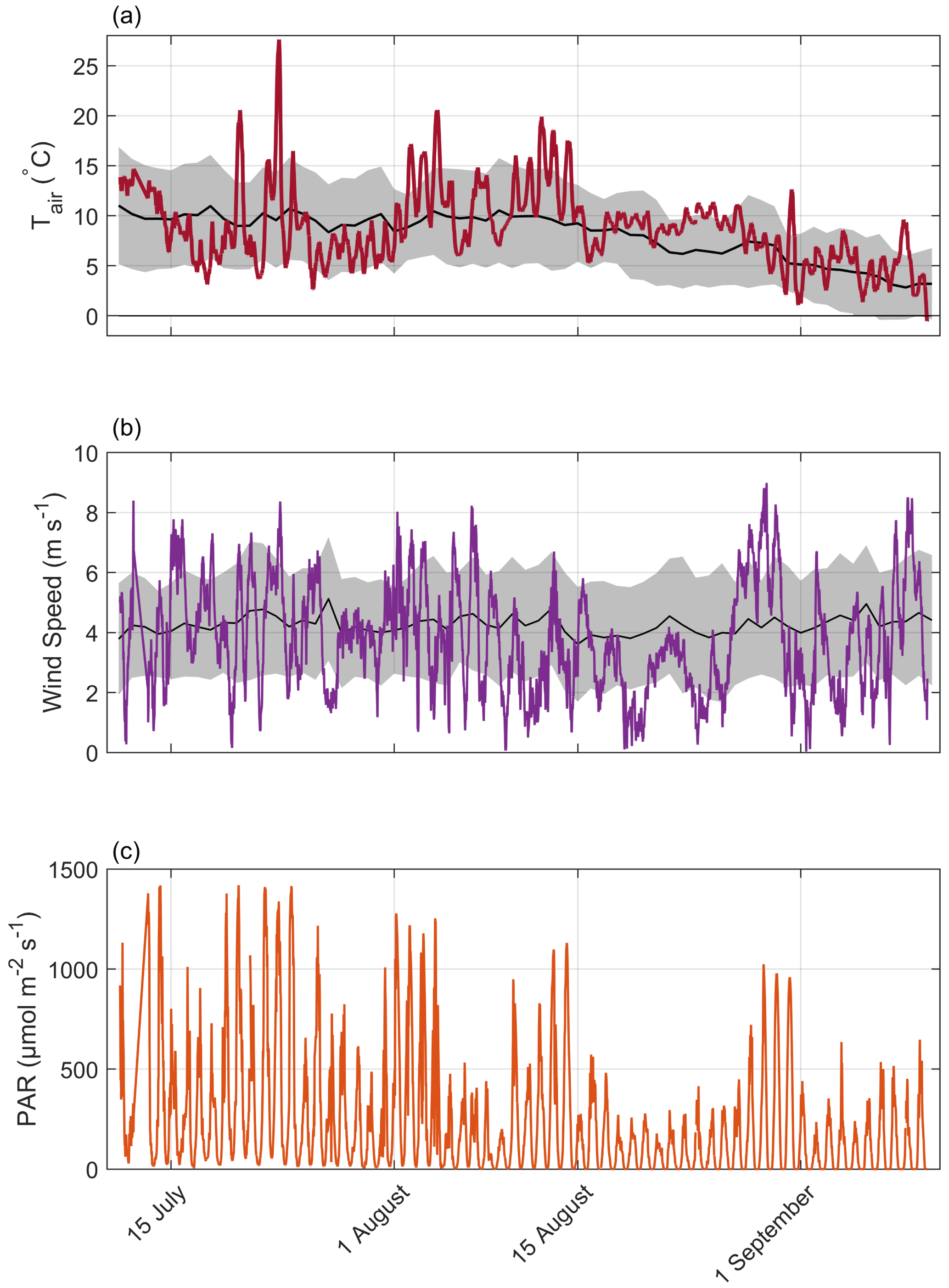
Figure A2Timeline of observed meteorological conditions during the observation period (2019) with air temperature at 2 m height (a), wind speed at 3 m height (b), and photosynthetically active radiation (PAR) (c). Mean values and standard deviation of observations during the past 16 years are plotted as black lines and gray areas.
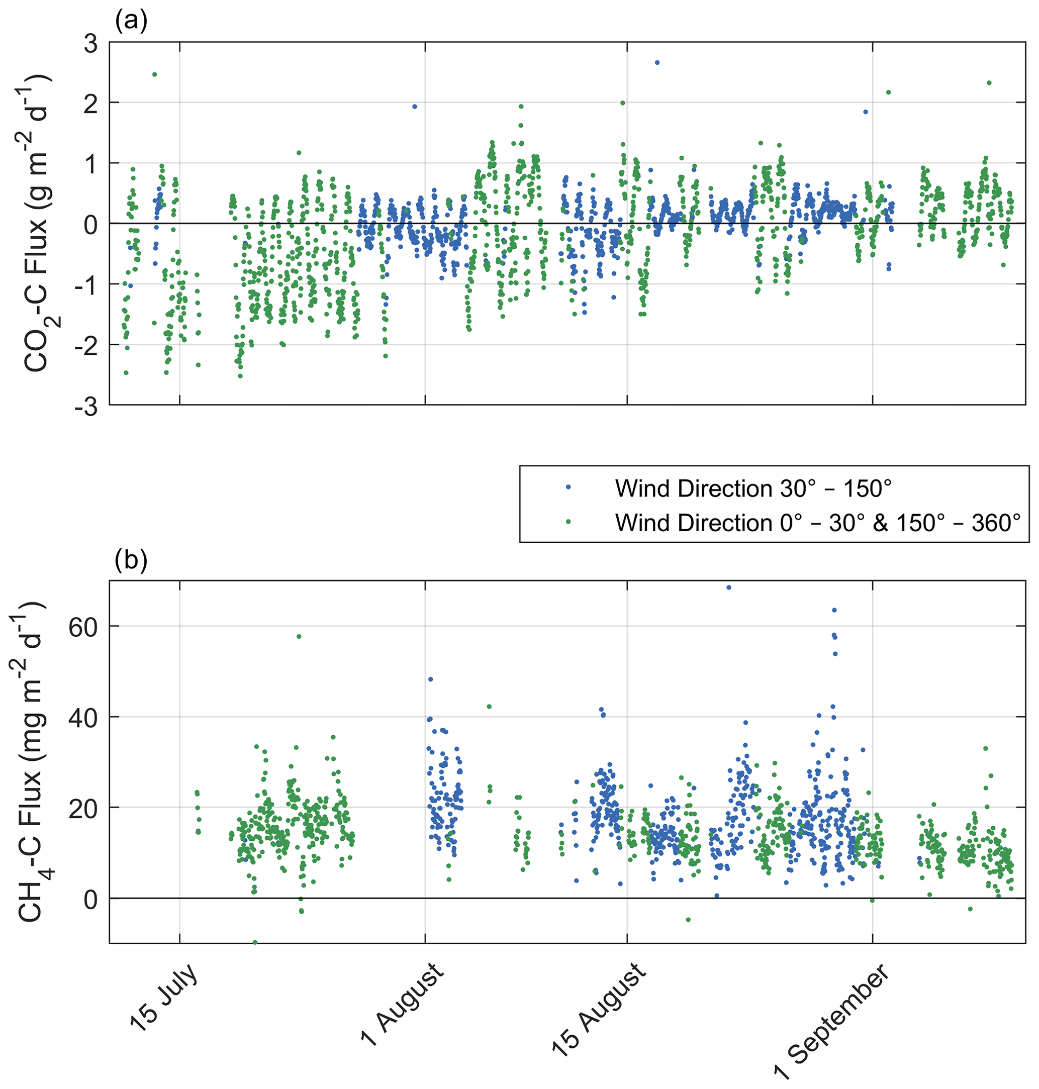
Figure A3Time series of 30 min observed CO2–C flux intervals (a) and CH4–C flux (b) with a quality flag of 0 or 1. The blue color represents fluxes originating from the wind direction of the merged polygonal pond (30–150∘ wind direction, mostly mixed signals from semi-terrestrial tundra and the surface of the merged polygonal pond), and the green color represents fluxes originating from all other wind directions.
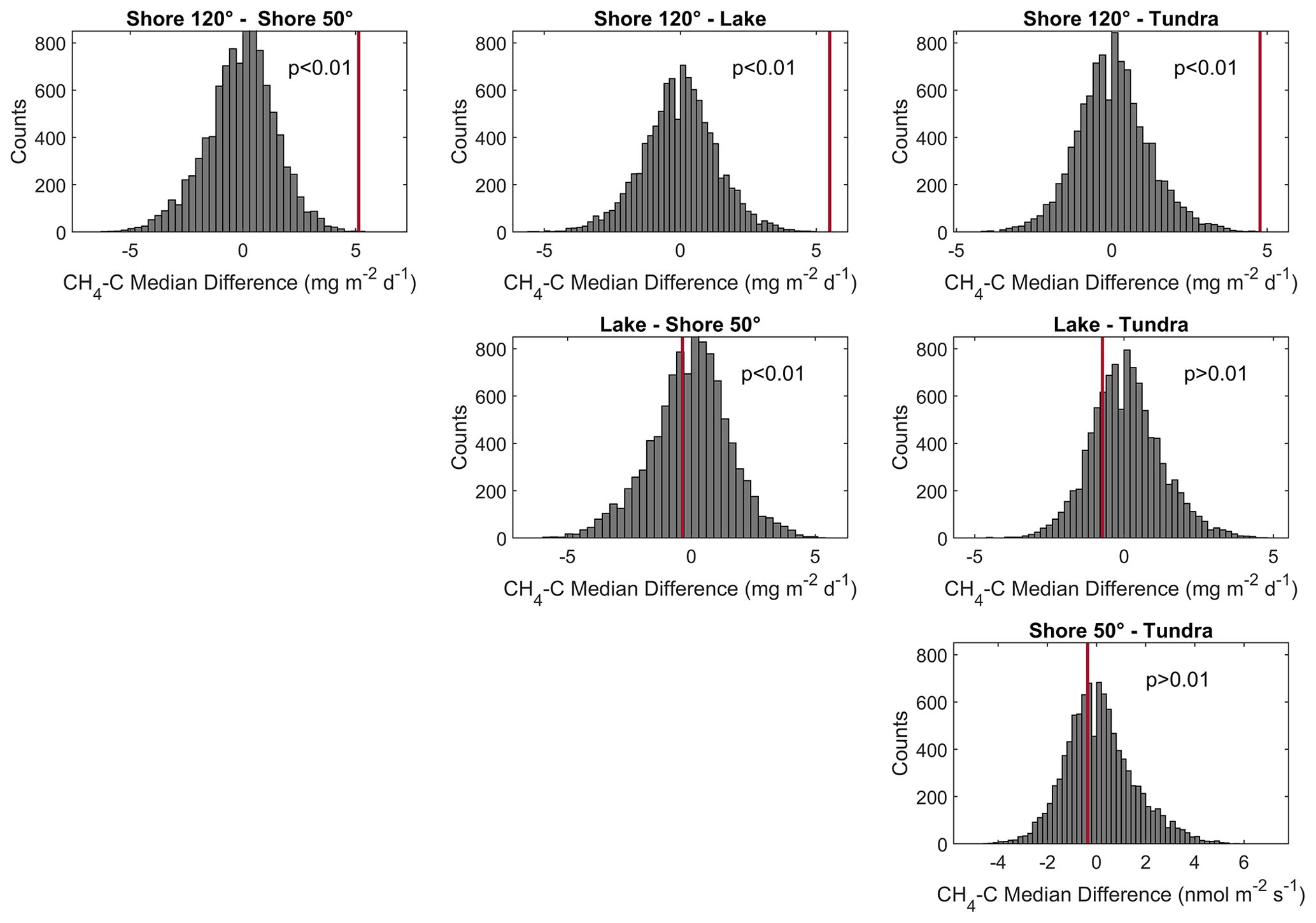
Figure A4Histogram of permutation tests between the medians of CH4 emissions from different wind direction classes in Fig. 6. All medians from flux observations during moderate wind-speed conditions. The observed differences in medians between the different wind direction classes are shown in red vertical bars in each plot.
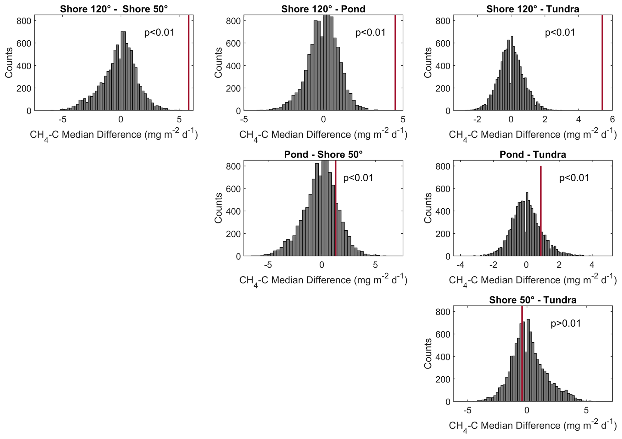
Figure A5Histogram of permutation tests between the medians of CH4 emissions from different wind direction classes in Fig. 6. All medians from flux observations during moderate air temperature conditions. The observed differences in medians between the different wind direction classes are shown in red vertical bars in each plot.
The data have been published at PANGAEA (https://doi.org/10.1594/PANGAEA.937594, Beckebanze et al., 2021). Code can be requested from the authors.
ZR and LK designed the experiments; ZR and LB carried out the fieldwork. ZR, LB, and LK developed the idea for the analysis, and CW and LB prepared the data. The formal analysis and data visualization were performed by LB and ZR with supervision by DH and LK. Resources (land-cover classification) have been provided by CM. LB and ZR prepared the manuscript with contributions from all co-authors.
The contact author has declared that neither they nor their co-authors have any competing interests.
Publisher’s note: Copernicus Publications remains neutral with regard to jurisdictional claims in published maps and institutional affiliations.
The authors thank Norman Rüggen for his tireless support before and remotely during the fieldwork; Anna Zaplavnova, Andrei Astapov, and Waldemar Schneider for their equally tireless support in the field; Andrei Astapov and Katya Abramova for additional pictures in the field; Volkmar Assmann and the station crew of Samoylov Island for their logistical support; and Sarah Wiesner, Leonardo Galera, and Tim Eckahardt for fruitful discussions during the data analysis. Also, the authors thank the reviewers.
This study was funded by the Deutsche Forschungsgemeinschaft (DFG, German Research Foundation) under Germany's Excellence Strategy – EXC 2037 “CLICCS – Climate, Climatic Change, and Society” – Project Number: 390683824, contribution to the Center for Earth System Research and Sustainability (CEN) of Universität Hamburg, and by the Bundesministerium für Bildung und Forschung KoPf project (grant 03F0764A).
This paper was edited by Andreas Ibrom and reviewed by two anonymous referees.
Abnizova, A., Siemens, J., Langer, M., and Boike, J.: Small ponds with major impact: The relevance of ponds and lakes in permafrost landscapes to carbon dioxide emissions, Global Biogeochem. Cy., 26, GB2041, https://doi.org/10.1029/2011gb004237, 2012. a, b, c, d, e, f, g, h, i, j, k, l, m
Andresen, C. G. and Lougheed, V. L.: Disappearing Arctic tundra ponds: Fine-scale analysis of surface hydrology in drained thaw lake basins over a 65 year period (1948–2013), J. Geophys. Res.-Biogeo., 120, 466–479, https://doi.org/10.1002/2014jg002778, 2015. a
Andresen, C. G., Lara, M. J., Tweedie, C. E., and Lougheed, V. L.: Rising plant-mediated methane emissions from arctic wetlands, Glob. Change Biol., 120.3, 466–479, https://doi.org/10.1111/gcb.13469, 2017. a
Beckebanze, L., Rehder, Z., Norman, R., Holl, D., Mirbach, C., Wille, C., and Kutzbach, L.: Eddy-covariance and meteorological measurements of large pond and polygonal tundra in Lena River Delta, Siberia (summer 2019), PANGAEA [data set], https://doi.org/10.1594/PANGAEA.937594, 2021. a
Bogard, M. J., del Giorgio, P. A., Boutet, L., Chaves, M. C. G., Prairie, Y. T., Merante, A., and Derry, A. M.: Oxic water column methanogenesis as a major component of aquatic CH4 fluxes, Nat. Commun., 5, 5350, https://doi.org/10.1038/ncomms6350, 2014. a
Boike, J., Grüber, M., Langer, M., Piel, K., and Scheritz, M.: Orthomosaic of Samoylov Island, Lena Delta, Siberia, PANGAEA, https://doi.org/10.1594/PANGAEA.786073, 2012. a
Boike, J., Georgi, C., Kirilin, G., Muster, S., Abramova, K., Fedorova, I., Chetverova, A., Grigoriev, M. N., Bornemann, N., and Langer, M.: Temperature, water level and bathymetry of thermokarst lakes in the continuous permafrost zone of northern Siberia – Lena River Delta, Siberia, PANGAEA, https://doi.org/10.1594/PANGAEA.846525, 2015a. a, b, c
Boike, J., Veh, G., Stoof, G., Grüber, M., Langer, M., and Muster, S.: Visible and near-infrared orthomosaic and orthophotos of Samoylov Island, Siberia, summer 2008, with links to data files, PANGAEA, https://doi.org/10.1594/PANGAEA.847343, 2015b. a, b
Boike, J., Veh, G., Viitanen, L.-K., Bornemann, N., Stoof, G., and Muster, S.: Visible and near-infrared orthomosaic of Samoylov Island, Siberia, summer 2015 (5.3 GB), PANGAEA, https://doi.org/10.1594/PANGAEA.845724, 2015c. a, b
Boike, J., Nitzbon, J., Anders, K., Grigoriev, M. N., Bolshiyanov, D. Y., Langer, M., Lange, S., Bornemann, N., Morgenstern, A., Schreiber, P., Wille, C., Chadburn, S., Gouttevin, I., and Kutzbach, L.: Meteorologic data at station Samoylov (2002–2018, level 2, version 201908), PANGAEA, https://doi.org/10.1594/PANGAEA.905232, 2019. a
Borrel, G., Jézéquel, D., Biderre-Petit, C., Morel-Desrosiers, N., Morel, J.-P., Peyret, P., Fonty, G., and Lehours, A.-C.: Production and consumption of methane in freshwater lake ecosystems, Res. Microbiol., 162, 832–847, https://doi.org/10.1016/j.resmic.2011.06.004, 2011. a
Bouchard, F., Laurion, I., Preskienis, V., Fortier, D., Xu, X., and Whiticar, M. J.: Modern to millennium-old greenhouse gases emitted from ponds and lakes of the Eastern Canadian Arctic (Bylot Island, Nunavut), Biogeosciences, 12, 7279–7298, https://doi.org/10.5194/bg-12-7279-2015, 2015. a, b, c, d
Bring, A., Fedorova, I., Dibike, Y., Hinzman, L., Mard, J., Mernild, S. H., Prowse, T., Semenova, O., Stuefer, S. L., and Woo, M. K.: Arctic terrestrial hydrology: A synthesis of processes, regional effects, and research challenges, J. Geophys. Res.-Biogeo., 121, 621–649, https://doi.org/10.1002/2015jg003131, 2016. a
Burba, G., Schmidt, A., Scott, R. L., Nakai, T., Kathilankal, J., Fratini, G., Hanson, C., Law, B., Mcdermitt, D. K., Eckles, R., Furtaw, M., and Velgersdyk, M.: Calculating CO2 and H2O eddy covariance fluxes from an enclosed gas analyzer using an instantaneous mixing ratio, Glob. Change Biol., 18, 385–399, https://doi.org/10.1111/j.1365-2486.2011.02536.x, 2012. a
Conrad, R.: Contribution of hydrogen to methane production and control of hydrogen concentrations in methanogenic soils and sediments, FEMS Microbiol. Ecol., 28, 193–202, https://doi.org/10.1016/S0168-6496(98)00086-5, 1999. a
Donis, D., Flury, S., Stöckli, A., Spangenberg, J. E., Vachon, D., and McGinnis, D. F.: Full-scale evaluation of methane production under oxic conditions in a mesotrophic lake, Nat. Commun., 8, 1661, https://doi.org/10.1038/s41467-017-01648-4, 2017. a
Ducharme-Riel, V., Vachon, D., del Giorgio, P. A., and Prairie, Y. T.: The relative contribution of winter under-ice and summer hypolimnetic CO2 accumulation to the annual CO2 emissions from northern lakes, Ecosystems, 18, 547–559, https://doi.org/10.1007/s10021-015-9846-0, 2015. a
Edgington, E. and Onghena, P.: Randomization tests, CRC Press, ISBN 9780367577711, 2007. a
Ellis, C. J., Rochefort, L., Gauthier, G., and Pienitz, R.: Paleoecological evidence for transitions between contrasting landforms in a polygon-patterned high arctic wetland, Arct. Antarct. Alp. Res., 40, 624–637, https://doi.org/10.1657/1523-0430(07-059)[ELLIS]2.0.CO;2, 2008. a
Encinas Fernández, J., Peeters, F., and Hofmann, H.: On the methane paradox: Transport from shallow water zones rather than in situ methanogenesis is the major source of CH4 in the open surface water of lakes, J. Geophys. Res.-Biogeo., 121, 2717–2726, https://doi.org/10.1002/2016JG003586, 2016. a
Eugster, W., Kling, G., Jonas, T., McFadden, J. P., Wüest, A., MacIntyre, S., and Chapin, F. S.: CO2 exchange between air and water in an Arctic Alaskan and midlatitude Swiss lake: Importance of convective mixing, J. Geophys. Res.-Atmos., 108, 4362, https://doi.org/10.1029/2002JD002653, 2003. a, b, c
Fan, S.-M., Wofsy, S. C., Bakwin, P. S., Jacob, D. J., and Fitzjarrald, D. R.: Atmosphere-biosphere exchange of CO2 and O3 in the central Amazon Forest, J. Geophys. Res.-Atmos., 95, 16851–16864, https://doi.org/10.1029/JD095iD10p16851, 1990. a
Fratini, G., Ibrom, A., Arriga, N., Burba, G., and Papale, D.: Relative humidity effects on water vapour fluxes measured with closed-path eddy-covariance systems with short sampling lines, Agr. Forest Meteorol., 165, 53–63, https://doi.org/10.1016/j.agrformet.2012.05.018, 2012. a
Gash, J. H. C. and Culf, A. D.: Applying a linear detrend to eddy correlation data in realtime, Bound.-Lay. Meteorol., 79, 301–306, https://doi.org/10.1007/bf00119443, 1996. a
Günthel, M., Klawonn, I., Woodhouse, J., Bižić, M., Ionescu, D., Ganzert, L., Kümmel, S., Nijenhuis, I., Zoccarato, L., Grossart, H.-P., and Tang, K. W.: Photosynthesis-driven methane production in oxic lake water as an important contributor to methane emission, Limnol. Oceanogr., 65, 2853–2865, https://doi.org/10.1002/lno.11557, 2020. a
Hedderich, R. and Whitman, W. B.: Physiology and biochemistry of the methane-producing Archaea, Springer New York, New York, NY, 1050–1079, https://doi.org/10.1007/0-387-30742-7_34, 2006. a, b
Holgerson, M. A. and Raymond, P. A.: Large contribution to inland water CO2 and CH4 emissions from very small ponds, Nat. Geosci., 9, 222–226, https://doi.org/10.1038/ngeo2654, 2016. a, b, c
Holl, D., Pancotto, V., Heger, A., Camargo, S. J., and Kutzbach, L.: Cushion bogs are stronger carbon dioxide net sinks than moss-dominated bogs as revealed by eddy covariance measurements on Tierra del Fuego, Argentina, Biogeosciences, 16, 3397–3423, https://doi.org/10.5194/bg-16-3397-2019, 2019. a
Ibrom, A., Dellwik, E., Flyvbjerg, H., Jensen, N. O., and Pilegaard, K.: Strong low-pass filtering effects on water vapour flux measurements with closed-path eddy correlation systems, Agr. Forest Meteorol., 147, 140–156, https://doi.org/10.1016/j.agrformet.2007.07.007, 2007a. a
Ibrom, A., Dellwik, E., Larsen, S. E., and Pilegaard, K.: On the use of the Webb-Pearman-Leuning theory for closed-path eddy correlation measurements, Tellus B, 59, 937–946, https://doi.org/10.1111/j.1600-0889.2007.00311.x, 2007b. a
Iwata, H., Hirata, R., Takahashi, Y., Miyabara, Y., Itoh, M., and Iizuka, K.: Partitioning eddy-covariance methane fluxes from a shallow lake into diffusive and ebullitive fluxes, Bound.-Lay. Meteorol., 169, 413–428, https://doi.org/10.1007/s10546-018-0383-1, 2018. a
Jammet, M., Dengel, S., Kettner, E., Parmentier, F.-J. W., Wik, M., Crill, P., and Friborg, T.: Year-round CH2 and CO2 flux dynamics in two contrasting freshwater ecosystems of the subarctic, Biogeosciences, 14, 5189–5216, https://doi.org/10.5194/bg-14-5189-2017, 2017. a, b, c, d, e, f, g
Jansen, J., Thornton, B. F., Jammet, M. M., Wik, M., Cortés, A., Friborg, T., MacIntyre, S., and Crill, P. M.: Climate-sensitive controls on large spring emissions of CH4 and CO2 from northern lakes, J. Geophys. Res.-Biogeo., 124, 2379–2399, https://doi.org/10.1029/2019JG005094, 2019. a, b
Jonsson, A., Åberg, J., Lindroth, A., and Jansson, M.: Gas transfer rate and CO2 flux between an unproductive lake and the atmosphere in northern Sweden, J. Geophys. Res.-Biogeo., 113, 1–13, https://doi.org/10.1029/2008JG000688, 2008. a, b
Kaimal, J. C. and Finnigan, J. J.: Atmospheric boundary layer flows: their structure and measurement, Oxford University Press, https://doi.org/10.1093/oso/9780195062397.001.0001, 1994. a
Kartoziia, A.: Assessment of the ice wedge polygon current state by means of UAV imagery analysis (Samoylov Island, the Lena Delta), Remote Sens., 11, 1627, https://doi.org/10.3390/rs11131627, 2019. a
Kling, G. W., Kipphut, G. W., and Miller, M. C.: The flux of CO2 and CH4 from lakes and rivers in arctic Alaska, Hydrobiologia, 240, 23–36, https://doi.org/10.1007/BF00013449, 1992. a
Knoblauch, C., Spott, O., Evgrafova, S., Kutzbach, L., and Pfeiffer, E. M.: Regulation of methane production, oxidation, and emission by vascular plants and bryophytes in ponds of the northeast Siberian polygonal tundra, J. Geophys. Res.-Biogeo., 120, 2525–2541, https://doi.org/10.1002/2015jg003053, 2015. a
Kormann, R. and Meixner, F. X.: An analytical footprint model for non-neutral stratification, Bound.-Lay. Meteorol., 99, 207–224, https://doi.org/10.1023/A:1018991015119, 2001. a, b, c, d
Kuhn, M., Lundin, E. J., Giesler, R., Johansson, M., and Karlsson, J.: Emissions from thaw ponds largely offset the carbon sink of northern permafrost wetlands, Sci. Rep., 8, 1–7, https://doi.org/10.1038/s41598-018-27770-x, 2018. a, b, c, d, e
LI-COR: EddyPro Version 7.0.6, https://www.licor.com/env/support/EddyPro/home.html (last access: 10 June 2020), 2019. a
Liss, P. S. and Slater, P. G.: Flux of gases across the Air-Sea interface, Nature, 247, 181–184, https://doi.org/10.1038/247181a0, 1974. a
Lundin, E. J., Giesler, R., Persson, A., Thompson, M. S., and Karlsson, J.: Integrating carbon emissions from lakes and streams in a subarctic catchment, J. Geophys. Res.-Biogeo., 118, 1200–1207, https://doi.org/10.1002/jgrg.20092, 2013. a
MATLAB: MATLAB Software 2019b, the MathWorks, Natick, MA, USA, https://mathworks.com, 2019. a, b
Mauder, M. and Foken, T.: Documentation and instruction manual of the eddy covariance software package TK2, Univ, Bayreuth, Abt. Mikrometeorol., Universität Bayreuth, Abt. Mikrometeorologie, ISSN 161489166.26, 26–42, 2004. a
McGuire, A. D., Christensen, T. R., Hayes, D., Heroult, A., Euskirchen, E., Kimball, J. S., Koven, C., Lafleur, P., Miller, P. A., Oechel, W., Peylin, P., Williams, M., and Yi, Y.: An assessment of the carbon balance of Arctic tundra: Comparisons among observations, process models, and atmospheric inversions, Biogeosciences, 9, 3185–3204, https://doi.org/10.5194/bg-9-3185-2012, 2012. a
Moncrieff, J., Clement, R., Finnigan, J., and Meyers, T.: Averaging, detrending, and filtering of eddy covariance time series, in: Handbook of micrometeorology, Springer, 7–31, https://doi.org/10.1007/1-4020-2265-4_2, 2004. a
Muster, S., Langer, M., Heim, B., Westermann, S., and Boike, J.: Subpixel heterogeneity of ice-wedge polygonal tundra: a multi-scale analysis of land cover and evapotranspiration in the Lena River Delta, Siberia, Tellus B, 64, 17301, https://doi.org/10.3402/tellusb.v64i0.17301, 2012. a, b, c, d, e
Muster, S., Roth, K., Langer, M., Lange, S., Cresto Aleina, F., Bartsch, A., Morgenstern, A., Grosse, G., Jones, B., Sannel, A. B. K., Sjöberg, Y., Günther, F., Andresen, C., Veremeeva, A., Lindgren, P. R., Bouchard, F., Lara, M. J., Fortier, D., Charbonneau, S., Virtanen, T. A., Hugelius, G., Palmtag, J., Siewert, M. B., Riley, W. J., Koven, C. D., and Boike, J.: PeRL: a circum-Arctic Permafrost Region Pond and Lake database, Earth Syst. Sci. Data, 9, 317–348, https://doi.org/10.5194/essd-9-317-2017, 2017. a
Neff, J. C. and Asner, G. P.: Dissolved organic carbon in terrestrial ecosystems: Synthesis and a model, Ecosystems, 4, 29–48, https://doi.org/10.1007/s100210000058, 2001. a
Peeters, F., Encinas Fernandez, J., and Hofmann, H.: Sediment fluxes rather than oxic methanogenesis explain diffusive CH4 emissions from lakes and reservoirs, Sci. Rep., 9, 243, https://doi.org/10.1038/s41598-018-36530-w, 2019. a
Ramsar Convention Secretariat: An introduction to the ramsar convention on wetlands (previously The Ramsar Convention Manual), Ramsar Convention Secretariat, Gland, Switzerland, https://www.ramsar.org/sites/default/files/documents/library/handbook1_5ed_introductiontoconvention_e.pdf (last access: 22 February 2022), 2016. a
Rehder, Z., Zaplavnova, A., and Kutzbach, L.: Identifying drivers behind spatial variability of methane concentrations in East Siberian ponds, Front. Earth Sci., 9, 617662, https://doi.org/10.3389/feart.2021.617662, 2021. a, b, c, d, e
Repo, M. E., Huttunen, J. T., Naumov, A. V., Chichulin, A. V., Lapshina, E. D., Bleuten, W., and Martikainen, P. J.: Release of CO2 and CH4 from small wetland lakes in western Siberia, Tellus B, 59, 788–796, https://doi.org/10.1111/j.1600-0889.2007.00301.x, 2007. a
Rößger, N., Wille, C., Holl, D., Göckede, M., and Kutzbach, L.: Scaling and balancing carbon dioxide fluxes in a heterogeneous tundra ecosystem of the Lena River Delta, Biogeosciences, 16, 2591–2615, https://doi.org/10.5194/bg-16-2591-2019, 2019a. a, b
Rößger, N., Wille, C., Veh, G., Boike, J., and Kutzbach, L.: Scaling and balancing methane fluxes in a heterogeneous tundra ecosystem of the Lena River Delta, Agr. Forest Meteorol., 266/267, 243–255, https://doi.org/10.1016/j.agrformet.2018.06.026, 2019b. a, b
Runkle, B. R., Sachs, T., Wille, C., Pfeiffer, E. M., and Kutzbach, L.: Bulk partitioning the growing season net ecosystem exchange of CO2 in Siberian tundra reveals the seasonality of it carbon sequestration strength, Biogeosciences, 10, 1337–1349, https://doi.org/10.5194/bg-10-1337-2013, 2013. a
Sepulveda-Jauregui, A., Walter Anthony, K. M., Martinez-Cruz, K., Greene, S., and Thalasso, F.: Methane and carbon dioxide emissions from 40 lakes along a north-south latitudinal transect in Alaska, Biogeosciences, 12, 3197–3223, https://doi.org/10.5194/bg-12-3197-2015, 2015. a, b, c
Sieczko, A. K., Duc, N. T., Schenk, J., Pajala, G., Rudberg, D., Sawakuchi, H. O., and Bastviken, D.: Diel variability of methane emissions from lakes, P. Natl. Acad. Sci. USA, 117, 21488–21494, https://doi.org/10.1073/pnas.2006024117, 2020. a, b
Squires, M. M. and Lesack, L. F.: The relation between sediment nutrient content and macrophyte biomass and community structure along a water transparency gradient among lakes of the Mackenzie Delta, Can. J. Fish. Aquat. Sci., 60, 333–343, https://doi.org/10.1139/f03-027, 2003. a
Treat, C. C., Marushchak, M. E., Voigt, C., Zhang, Y., Tan, Z., Zhuang, Q., Virtanen, T. A., Räsänen, A., Biasi, C., Hugelius, G., Kaverin, D., Miller, P. A., Stendel, M., Romanovsky, V., Rivkin, F., Martikainen, P. J., and Shurpali, N. J.: Tundra landscape heterogeneity, not interannual variability, controls the decadal regional carbon balance in the Western Russian Arctic, Glob. Change Biol., 24, 5188–5204, https://doi.org/10.1111/gcb.14421, 2018. a, b, c
Tuovinen, J.-P., Aurela, M., Hatakka, J., Räsänen, A., Virtanen, T., Mikola, J., Ivakhov, V., Kondratyev, V., and Laurila, T.: Interpreting eddy covariance data from heterogeneous Siberian tundra: land-cover-specific methane fluxes and spatial representativeness, Biogeosciences, 16, 255–274, https://doi.org/10.5194/bg-16-255-2019, 2019. a, b
Earth Resources Observation and Science (EROS) Center: USGS EROS Archive – Declassified Data – Declassified Satellite Imagery – 1, https://www.usgs.gov/centers/eros/science/usgs-eros-archive-declassified-data-declassified-satellite-imagery-1?qt-science_center_objects=0#science (last access: 15 June 2020), 2018. a
Vickers, D. and Mahrt, L.: Quality control and flux sampling problems for tower and aircraft data, J. Atmos. Ocean. Technol., 14, 512–526, https://doi.org/10.1175/1520-0426(1997)014<0512:QCAFSP>2.0.CO;2, 1997. a
Vonk, J. E., Tank, S. E., Bowden, W. B., Laurion, I., Vincent, W. F., Alekseychik, P., Amyot, M., Billet, M. F., Canário, J., Cory, R. M., Deshpande, B. N., Helbig, M., Jammet, M., Karlsson, J., Larouche, J., Macmillan, G., Rautio, M., Walter Anthony, K. M., and Wickland, K. P.: Reviews and syntheses: Effects of permafrost thaw on Arctic aquatic ecosystems, Biogeosciences, 12, 7129–7167, https://doi.org/10.5194/bg-12-7129-2015, 2015. a, b
Walter, K. M., Zimov, S. A., Chanton, J. P., Verbyla, D., and Chapin, F. S.: Methane bubbling from Siberian thaw lakes as a positive feedback to climate warming, Nature, 443, 71–75, https://doi.org/10.1038/nature05040, 2006. a, b
Walter Anthony, K. M. and Anthony, P.: Constraining spatial variability of methane ebullition seeps in thermokarst lakes using point process models, J. Geophys. Res.-Biogeo., 118, 1015–1034, https://doi.org/10.1002/jgrg.20087, 2013. a
Webb, E. K., Pearman, G. I., and Leuning, R.: Correction of flux measurements for density effects due to heat and water vapour transfer, Quarterly J. Roy. Meteorol. Soc., 106, 85–100, https://doi.org/10.1002/qj.49710644707, 1980. a
Wik, M., Varner, R. K., Anthony, K. W., MacIntyre, S., and Bastviken, D.: Climate-sensitive northern lakes and ponds are critical components of methane release, Nat. Geosci., 9, 99–105, https://doi.org/10.1038/ngeo2578, 2016. a, b, c, d, e