the Creative Commons Attribution 4.0 License.
the Creative Commons Attribution 4.0 License.
 | 05 Apr 2022
Examining the role of environmental memory in the predictability of carbon and water fluxes across Australian ecosystems
Martin G. De Kauwe
Gab Abramowitz
Jamie Cleverly
Nina Hinko-Najera
Mark J. Hovenden
Yao Liu
Andy J. Pitman
Kiona Ogle
The vegetation's response to climate change is a significant source of uncertainty in future terrestrial biosphere model projections. Constraining climate–carbon cycle feedbacks requires improving our understanding of both the immediate and long-term plant physiological responses to climate. In particular, the timescales and strength of memory effects arising from both extreme events (i.e. droughts and heatwaves) and structural lags in the systems (such as delays between rainfall and peak plant water content or between a precipitation deficit and down-regulation of productivity) have largely been overlooked in the development of terrestrial biosphere models. This is despite the knowledge that plant responses to climatic drivers occur across multiple timescales (seconds to decades), with the impact of climate extremes resonating for many years.
Using data from 12 eddy covariance sites, covering two rainfall gradients (256 to 1491 mm yr−1) in Australia, in combination with a hierarchical Bayesian model, we characterised the timescales and magnitude of influence of antecedent drivers on daily net ecosystem exchange (NEE) and latent heat flux (λE). By focussing our analysis on a single continent (and predominately on a single genus), we reduced the degrees of variation between each site, providing a novel chance to explore the unique characteristics that might drive the importance of memory. Model fit varied considerably across sites when modelling NEE, with R2 values of between 0.30 and 0.83. λE was considerably more predictable across sites, with R2 values ranging from 0.56 to 0.93. When considered at a continental scale, both fluxes were more predictable when memory effects (expressed as lagged climate predictors) were included in the model. These memory effects accounted for an average of 17 % of the NEE predictability and 15 % for λE. Consistent with prior studies, the importance of environmental memory in predicting fluxes increased as site water availability declined (, p<0.01 for NEE, , p<0.05 for λE). However, these relationships did not necessarily hold when sites were grouped by vegetation type. We also tested a model of k-means clustering plus regression to confirm the suitability of the Bayesian model for modelling these sites. The k-means approach performed similarly to the Bayesian model in terms of model fit, demonstrating the robustness of the Bayesian framework for exploring the role of environmental memory. Our results underline the importance of capturing memory effects in models used to project future responses to climate change, especially in water-limited ecosystems. Finally, we demonstrate a considerable variation in individual-site predictability, driven to a notable degree by environmental memory, and this should be considered when evaluating model performance across ecosystems.
- Article
(383 KB) - Full-text XML
-
Supplement
(307 KB) - BibTeX
- EndNote


Ecosystems respond to climate at a wide range of timescales: stomata respond to changes in humidity within seconds (Fanjul and Jones, 1982), while extreme droughts can impact plant growth for up to 5 or more years after the event (Anderegg et al., 2015; Vanoni et al., 2016). There is growing interest in better understanding these timescales over which vegetation responds to environmental conditions, particularly when considering the projected rate of future climate change and threats this poses to ecosystem stability (Mottl et al., 2021). An increasing number of studies have demonstrated the importance of past events such as fires (Sun et al., 2020), land management (Seabloom et al., 2020), and droughts (Anderegg et al., 2015; Kannenberg et al., 2020) on current ecosystem behaviour, in many cases, over time spans of years.
It is important to differentiate between what shall be referred to as “legacy” and “lag” effects. The ongoing impacts of climate extremes are an example of the former – they leave a persistent yet diminishing “legacy” from their single occurrence. A “lagged” effect differs in that it is an ongoing, constant delay in reaction to current conditions. The differing response times of vegetation to stimuli mean that lags exist associated with climate and the exchange of heat, energy, and carbon fluxes between ecosystems and the atmosphere. For instance, current grassland soil respiration can be strongly influenced by antecedent moisture from the prior 2 weeks, with the importance of longer lags decreasing sharply despite cumulative lag effects showing for up to 6 weeks (Cable et al., 2013). These response timescales are affected by ecosystem characteristics, such as vegetation structure. Cable et al. (2013) also found that, relative to grasslands, shrublands had a much longer cumulative lag effect in soil respiration of up to 10 weeks, with the first 4 weeks being most important.
The timescale of responses also differs among ecosystem processes. Feldman et al. (2021) found a lag of 5 d between a pulse of rainfall and peak plant water content in semi-arid grasslands, which in turn is likely to affect plant water status and hence carbon uptake. In arid and semi-arid ecosystems, soil respiration can respond immediately to a rainfall pulse and remain elevated for up to 2 d, while net ecosystem exchange (NEE) rates have a lagged response of up to a week (Huxman et al., 2004; Cleverly et al., 2013). Cleverly et al. (2016) found a variety of lags for phenological and photosynthetic responses in central Australia, ranging from immediate to 6 weeks. Antecedent climate is yet another factor that influences ecosystem response timescales. Repeated droughts in one growing season can negatively affect a plant's investment in biomass in comparison to a single event (Lemoine et al., 2018). In semi-arid and arid regions, NDVI (normalised difference vegetation index, a measure of vegetation greenness) responds to precipitation with lags of up to 7 months, while less arid areas tend to have shorter response times (Liu et al., 2018). From a study over the entire state of Kansas, Wang et al. (2003) found shorter lags between NDVI and precipitation, with the strongest correlation being at a 4-week lag. In fact, antecedent conditions could even be more important than concurrent conditions when measuring ecosystem productivity (Sala et al., 2012). Clearly, there is a diverse range of lagged responses to climate found within terrestrial ecosystems. Confounding factors, such as differing vegetation characteristics (including the proportion of woody vegetation, rooting depth, and varying allocation strategies), prevailing climate, interacting processes, and prior extreme events, all influence the magnitude and timescale of these lags and their impact on ecosystem fluxes.
Despite increasing attention on the impact of these lags within ecosystems, they are poorly captured within terrestrial biosphere models (TBMs) (Anderegg et al., 2015; Frank et al., 2015; Ogle and Barber, 2016; Kannenberg et al., 2020). For example, TBMs usually have an instantaneous coupling between photosynthetic uptake and growth in plants, while in reality carbon is first allocated to non-structural carbohydrates, allowing it to sustain growth and respiratory demands during periods of lower photosynthetic activity (Fatichi et al., 2014; Smith and Dukes, 2013; Jones et al., 2020). Anderegg et al. (2015) similarly found that earth system models are generally weak at predicting the impact of droughts on productivity during the drought recovery period. Models generally overestimate the immediate impact and underestimate the recovery times for extreme events (Kolus et al., 2019; Huang et al., 2016; Ukkola et al., 2016a). Recent satellite observations have also indicated that models fail to capture the impact of water stored in reservoirs with longer response times to climate (such as deeper soil moisture, groundwater, and surface water), resulting in models being more dominated by anomalies at shorter timescales than observations (Humphrey et al., 2018). Such model failures may in part be due to incorrect rooting depths, poor soil profile characterisation, or a lack of representation of these long-term storage pools such as groundwater or wetlands. Implementing these “lagged effects” into the models used to predict the carbon cycle is key to improving their performance (Keenan et al., 2012).
To better incorporate the role of lags in model process representations, we first need to determine which physical processes are affected and then quantify the timescales at which lags persist. Frequently, autoregressive methods are used in studies looking at specific pre-determined timescales, such as the current year's productivity and/or the previous year's rainfall and productivity (Sala et al., 2012) or the prior 6 months of climate (Zhang et al., 2015). Many studies have however indicated that intra-annual rainfall patterns are more important to productivity than total annual rainfall (Hovenden et al., 2014, 2018). Overcoming these subjective constraints and still providing freedom to explore sensitivity to shorter (sub-yearly) lags seems key to revealing any unexpected behaviour and detailing the full extent of memory effects, including any potential interaction between climate drivers.
To address this issue of strictly prescribed lags, new statistical approaches have been developed that allow for more flexible estimation of timescales of influences and magnitudes of lag effects (Ogle et al., 2015). Such methods have identified a key role of memory effects in many ecosystem processes, including soil and ecosystem respiration (Ryan et al., 2015; Cable et al., 2013; Barron-Gafford et al., 2014) and gross primary production (Ryan et al., 2017). NEE and latent heat flux (λE) have also been shown to be influenced by these memory effects (Samuels-Crow et al., 2020), which are often stronger at drier sites (Liu et al., 2019).
Here we use the stochastic antecedent modelling (SAM) framework of Liu et al. (2019) to probe lagged flux responses in individual ecosystems across two environmental gradients in Australia. We explore whether a relationship between site aridity and importance of antecedent conditions holds when viewed at a smaller spatial scale or whether such a relationship is confounded by other site characteristics, such as vegetation structure or extreme weather conditions. By focusing on a number of intensively studied sites within a single continent and examining the relative contributions of various predictors in each environment, we aim to reduce these potential confounding factors. We include the sites of the North Australian Tropical Transect (NATT) as an explicit case study since this “living laboratory” covers a steep rainfall gradient without a correspondingly strong change in vegetation (Hutley et al., 2011). By applying the SAM framework to λE in addition to NEE, we explore how the timescales of response vary between these coupled fluxes, which can improve our understanding of the processes involved in environmental memory. Our second aim is to explore whether assessing the importance of environmental memory at a site can offer insights into TBM evaluation. If sites are more predictable or have a greater dependence on antecedent conditions (and therefore are traditionally less predictable), this should be taken into account when critically analysing TBM performance across sites. Finally, we examine an alternative statistical approach for antecedent modelling to test whether structural assumptions in the SAM framework notably affect inferences about environmental lags. In addition to highlighting sites with more complex lagged environmental behaviour (a tougher test for TBMs), explicit identification of individual lagged site mechanisms can highlight key processes missing from TBMs more broadly.
2.1 Datasets
2.1.1 Flux data
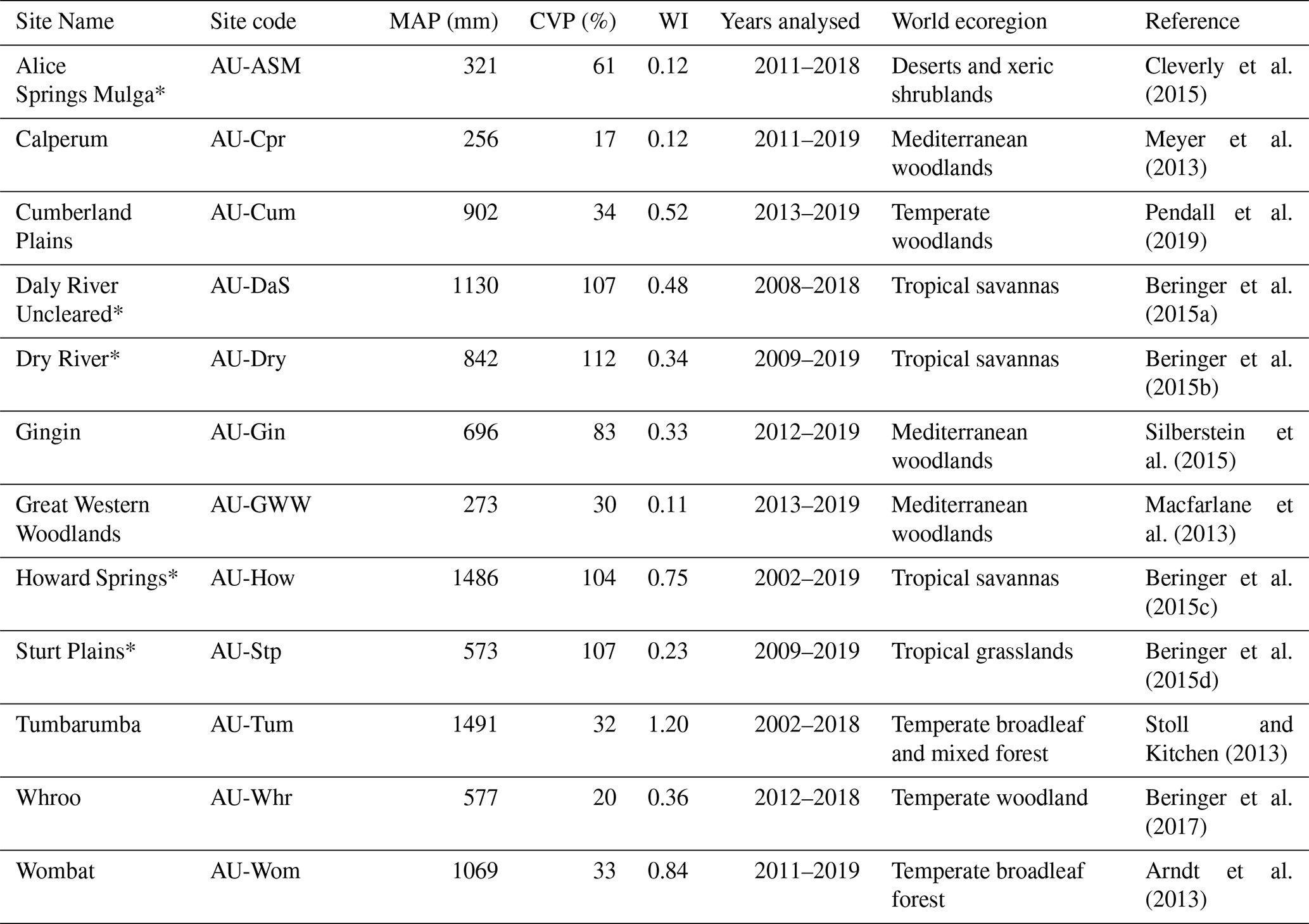
Meteorological and flux data were taken from the OzFlux data repository for 12 eddy covariance towers (see Table 1 for site details). The sites were selected to cover a variety of vegetation types and fall into two overarching groups. Firstly, sites comprising the North Australia Tropical Transect (NATT) were included. These vary from tropical grasslands to semi-arid shrublands and savannahs (International Geosphere–Biosphere Programme – IGBP – classifications of grassland, savannah, and woody savannah) along a steep rainfall gradient (321 to 1486 mm annual precipitation) running from north to south in the Northern Territory, Australia. Secondly, we grouped the southern Australian woodland sites (SAWSs). These were selected as sites with a greater proportion of woody vegetation than the NATT sites (IGBP classifications of savannah, woody savannah, and evergreen broadleaf forest) while still covering a broad range of climate types (256 to 1491 mm annual precipitation). While the vegetation differences between the groups are less distinguished at the drier sites, the NATT sites are considered “savannah” sites, and the SAWS sites are referred to as “woodland” sites.
Cleverly et al. (2015)Meyer et al. (2013)Pendall et al. (2019)Beringer et al. (2015a)Beringer et al. (2015b)Silberstein et al. (2015)Macfarlane et al. (2013)Beringer et al. (2015c)Beringer et al. (2015d)Stoll and Kitchen (2013)Beringer et al. (2017)Arndt et al. (2013)Table 1Site information for all sites included in the analysis. MAP is the mean annual precipitation at the site. CVP is the coefficient of variation in precipitation. WI is a wetness index of MAP over mean annual reference evapotranspiration. MAP, CVP, and WI are calculated from the WorldClim dataset, which covers 1970–2000 (Fick and Hijmans, 2017; Trabucco and Zomer, 2018). “Years analysed” corresponds to the full years of data available for analysis, inclusive. “World ecoregion” is the biome classification of each site, which is based on climatic regime and ecological structure, among other criteria (Olson et al., 2001; Beringer et al., 2016). Asterisks indicate sites that are part of the NATT. Litchfield was initially included in the analysis but was discarded due to the short time series available. All other sites are grouped as the SAWS. Data were obtained from the OzFlux Data Portal (http://data.ozflux.org.au, last access: 21 September 2020).
In this analysis we used observations of daily NEE and λE fluxes. NEE is a direct measurement of carbon exchange which represents the balance of carbon uptake and losses and is favoured over flux-derived gross primary productivity due to issues with respiration partitioning (Renchon et al., 2021). λE measures all evaporation, including contributions from soil and vegetation. Although carbon (uptake) and water fluxes are non-linearly coupled (De Kauwe et al., 2015a), NEE and λE are expected to exhibit a degree of independence in their responses to environmental conditions (including differing timescales) since they contain contributions from different components of the system (e.g. soil or understorey vs. canopy).
The fluxes were modelled using meteorological observations, which included mean downward short-wave radiation, mean air temperature, mean vapour pressure deficit (VPD), and precipitation. All OzFlux data were extracted at a half-hourly time step, aggregated to daily data, screened to only include complete calendar years, and then mean-centred. Sites were also screened to ensure that at least 5 years of good-quality data were available, which excluded five sites that have previously been included in the NATT (Adelaide River, Daly River Pasture, Fogg Dam, Litchfield, and Ti Tree East). Details on the data processing and quality control of OzFlux data can be found in Isaac et al. (2017). Here, we used the L6 data, which are quality-checked and gap-filled.
Normalised difference vegetation index (NDVI), a proxy for vegetation greenness, was obtained for each site from the global MODIS daily albedo data product at a 500 m resolution via the Google Earth Engine interface (Schaaf and Wang, 2015; Gorelick et al., 2017). This dataset is calculated at a daily time step based on a 16 d composite of observations. This is used in the Bayesian model as a measure of whether the sites were in a “growing” (higher greenness) or “dormant” (lower greenness) state (see below).
General site characteristics including the mean annual precipitation (MAP) and the coefficient of variation in precipitation (CVP) were obtained from the WorldClim dataset (Fick and Hijmans, 2017), while the wetness index (WI) was calculated from these data as MAP divided by mean annual potential evapotranspiration (Trabucco and Zomer, 2018; Zomer et al., 2007, 2008). This WI assumes that lower values indicate more water-limited locations, while higher values are locations with a greater proportion of precipitation to potential evaporation. These data were used in preference to meteorological data from individual sites as they cover a significantly long time period.
2.2 Analysis
2.2.1 Statistical analysis of memory and lags
Following previous work by Liu et al. (2019) in the application of the SAM framework, we separately model NEE and λE using a non-linear mixed-effect Bayesian model at each site. The same formulation was used to model both fluxes at the 12 sites, and so the following description of the NEE model is also applicable to λE modelling.
While the exact distribution of flux errors is site-dependent and can vary between superimposed Gaussian distributions (Lasslop et al., 2008) or Student's t distribution (Weber et al., 2018), daily NEE is assumed to be Laplace-distributed (Richardson et al., 2006) with mean μNEE and variance σ2 in line with Liu et al. (2019); μNEE at time t is modelled as per Eq. (1).
Gn and Dn represent two sets of coefficients, corresponding to “growing” and “dormant” behaviours, respectively. These two behaviours are a function of NDVI, which we used to capture a site's growing seasons. Growing season differences were accounted for in our statistical modelling because at many of the sites growth is restricted by water availability (e.g. following rain), which in Australia is not strictly related to a specific growth period during the year; ϕ(t) is a function that partitions between these two behaviours based on NDVI such that Dn is 1, and Gn is 0 at minimum NDVI and vice versa at maximum NDVI:
A uniform prior on the interval [−1, 1] is assigned to ϕ*. This ensures that ϕ(t) increases monotonically with increasing NDVI. The ϕ* value modifies this function, allowing either a one-to-one linear relationship (when ϕ* is equal to 0) or varying non-linear relationships. In this manner, the proportion of time steps assigned to predominately “growing” or “dormant” behaviour (when ϕ(t) takes a value greater than 0.5 or less than 0.5, respectively) is modified during the model fitting.
CLIMATEn(t) is a weighted sum of daily climate measurements with various lags, where n indicates various variables as follows. When n=1, CLIMATEn(t)=1 at all time steps t and is therefore an intercept term. Where n=2, 3, 4, or 5, CLIMATEn(t) represents the contribution of each of the short-term climate predictors (e.g. short-wave radiation, air temperature); n=6, …, 9 are the quadratic interactions of these predictors, and n=10, …,15 are the remaining pairwise interactions; n=16 is the contribution of long-term precipitation. Equation (3) is the generic form for a short-term climate predictor, where represents the weights assigned to the lagged climate observations CLIMn(t−lag). The CLIMATEn(t) terms for each n are summarised in Table 2.
Long-term precipitation (mean rainfall calculated over varying periods, up to 365 d prior; Table 3) is included as it is possible for the vegetation at these sites to be drawing on water reservoirs from deeper within the soil profile than would be recharged by short-term precipitation. This is especially true for the monsoonal sites along the NATT which experience prolonged dry seasons. In comparison, radiation, temperature, and VPD are assumed not to influence the fluxes at time spans longer than 14 d and so are restricted to the shorter timescale (Ryan et al., 2017).
Each CLIMATEn(t) term has a unique set of weights, which were assigned a Dirichlet prior. This ensures that each individual weight is constrained between 0 and 1, and the sum of the weights within each CLIMATEn(t) term is equal to 1. As such, each weight is indicative of the relative importance of the specific climate variable at the corresponding lag period.
To reduce the number of parameters estimated in the model, the lagged time steps in the short-term CLIMATEn(t) sums were grouped into blocks, with each lag in a block assigned the same weight, as shown in Table 3. For instance, the same weight is assigned to observations from 7 and 8 d prior. The decreasing resolution further into the past is due to the expectation that the importance of the driving variable on consecutive days becomes increasingly difficult to distinguish as the lag time increases. This reduction in the number of individual weights being estimated improves the model computation time and convergence.
Table 2Formulas for the CLIMATEn(t) term in the model for μNEE(t) for each n. TAS is mean air temperature, SWR is incoming short-wave radiation, VPD is vapour pressure deficit, and PPT is rainfall. The lag term in the sums is in days; i.e. at lag = 3, TAS(t−lag) is the mean air temperature from 3 d prior. Note that the lags in are larger periods than the daily lags for the short-term predictors, and PPT is here taken as the mean daily rainfall in these lagged periods; is the weight assigned to each lag period and is different for each of the five climate variables.
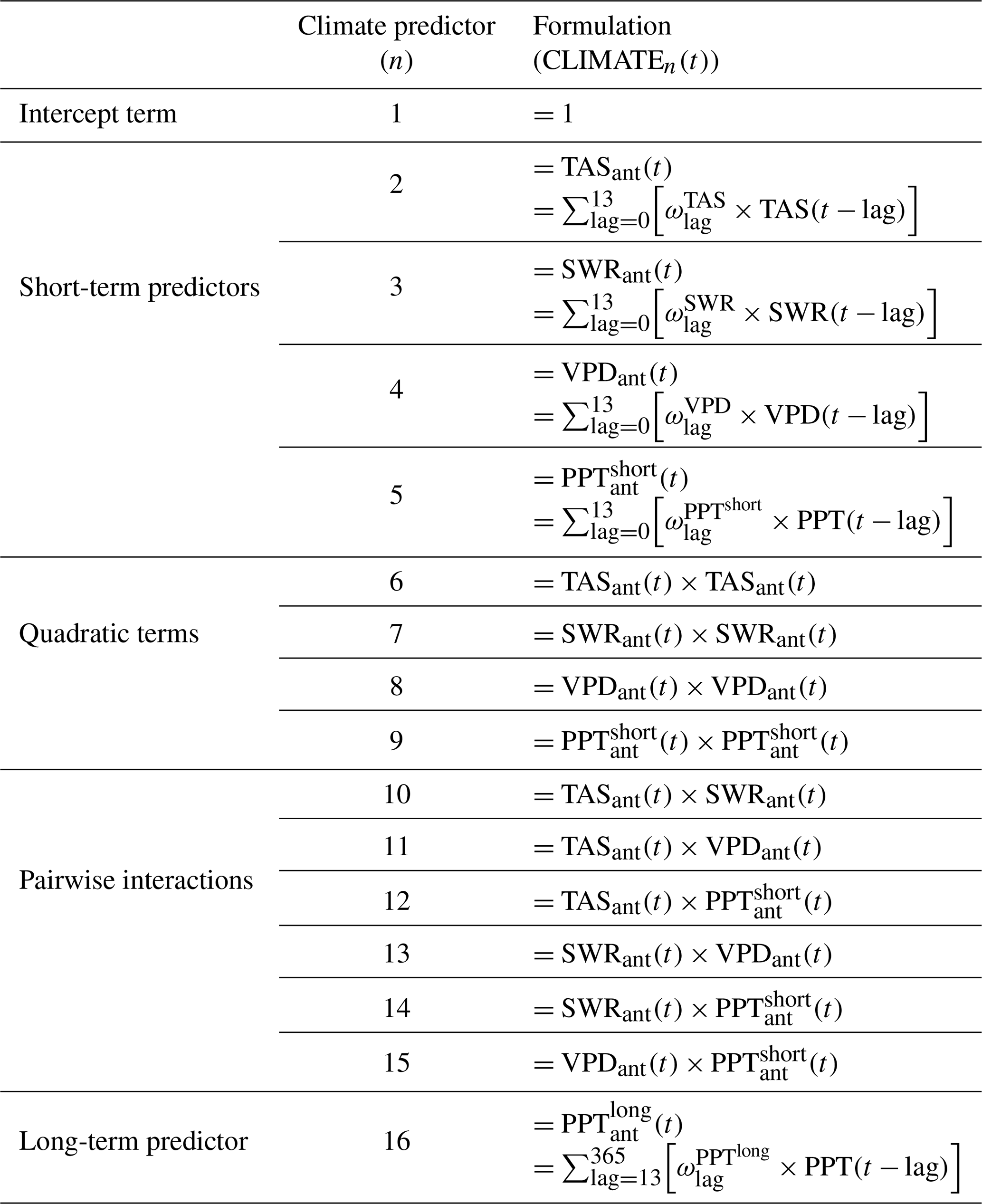
Table 3Assignment of weights to lagged periods. The same weight is applied to multiple lag periods for the short-term predictors. Grouping of lags is necessary to reduce the number of parameters being estimated by the Bayesian framework, which improves model computing performance and reduces the risk of overfitting.
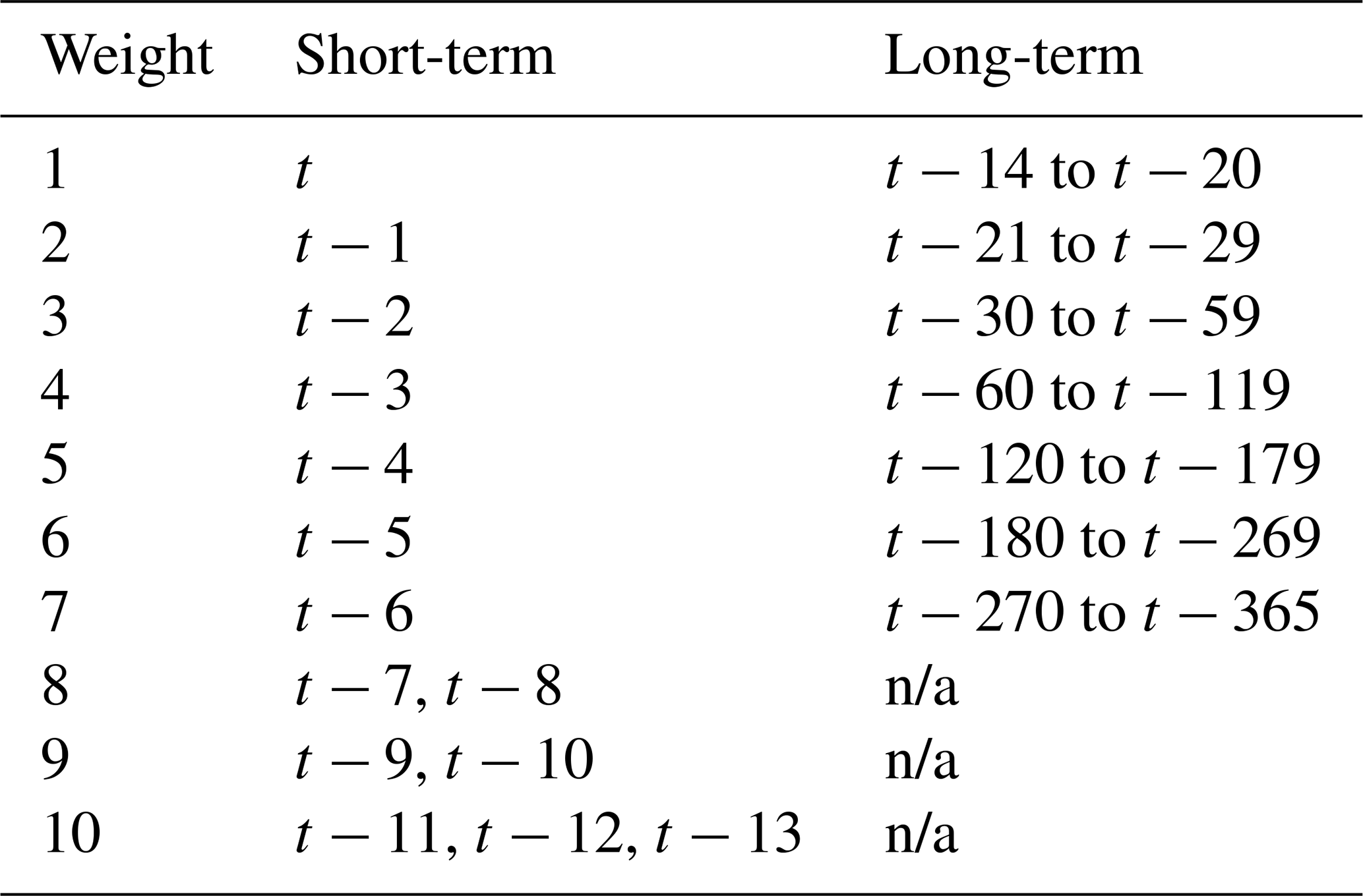
n/a: not applicable.
Significant changes between Liu et al. (2019) and our model include the removal of soil moisture, the introduction of shorter precipitation lags (<14 d), and min–max normalisation of NDVI on a per-site basis. We excluded soil moisture from our analysis due to inconsistencies in the data record at some sites as well as varying measurement depths across sites. Additionally, the soil moisture data are typically collected from relatively shallow depths of the soil profile and, as such, may not accurately reflect the root zone soil moisture in woody ecosystems. For instance, Eucalyptus species are known to have dimorphic rooting profiles with deep tap roots able to access water from below the shallow root zone (Knight, 1999). To account for short-term impacts of water availability following the removal of soil moisture, precipitation lags at the shorter timescales were introduced. Finally, NDVI is normalised to vary from 0 at minimum NDVI to 1 at maximum observed NDVI at each site for two reasons. Firstly, this ensures that each site spans the full range of ϕ values between “growing” (1) and “dormant” (0) periods. The similarity between the individual Gn and Dn coefficients was then able to indicate any differences between these two behaviours. Secondly, it was hypothesised that totally excluding coefficients of one behaviour at minimum NDVI (and the other at maximum NDVI) would improve convergence towards well-defined parameter values during model fitting.
The Bayesian model was implemented in JAGS via R, using the r2jags package and Markov chain Monte Carlo (MCMC) simulations (Plummer, 2003; R Core Team, 2020; Su and Yajima, 2020). Convergence of the MCMC chains was confirmed visually with trace plots and analytically with the Gelman–Rubin and Geweke diagnostic values as calculated with the coda package (Plummer et al., 2006). The MCMC iterations were set high enough to minimise the number of parameters with an “effective sample size” of less than 10 000, which ensured the parameters' posterior distributions were sufficiently sampled (Kruschke, 2015; Harms and Roebroeck, 2018).
Once converged, model performance was assessed using five metrics: coefficient of determination (R2), correlation coefficient (CCO), standard deviation difference (SDD), mean bias error (MBE), and normalised mean error (NME) (Haughton et al., 2016). These were calculated between the daily time series of the observed and modelled flux. Together, these metrics capture a broad range of potential model performance measures relative to the observations.
The model was first run in a “current climate only” configuration, referred to as the “CC model”, where the weights were set to 0 for all but the current-day climate (which were therefore assigned a weight of 1). This restriction was removed for a second set of model runs to utilise the full SAM framework. This second set of runs introduces “environmental memory” to the flux predictions, and so this model configuration is referred to as the “EM model”. Finally, in an attempt to capture any remaining predictability in the observations, the residuals from the EM models were themselves modelled using a standard autoregressive process with a time lag of 1 d, which is an AR(1) model. This effectively allows a correction of the predicted flux based on the prior error in the prediction. While previously this has been referred to as capturing a “biological memory” component, there are various plausible effects that this AR(1) model can be considered to represent (Liu et al., 2019). As such we do not claim it represents a specific memory process but rather a lower bound on site predictability, and it is simply referred to as the “AR model”.
2.2.2 Additional modelling
For comparison and confirmation of the SAM method, site NEE and λE were also modelled using an approach of k-means clustering plus regression (Abramowitz, 2012; Best et al., 2015). The k-means approach is an alternative in-sample empirical model, providing a direct comparison to the SAM approach. The clustering is performed on the environmental predictor variables, and the time steps that belong within each cluster are determined. For each cluster, a linear regression between the climate predictors and the flux at the time steps within the cluster is performed. This allows assessment of the degree to which SAM results are indicative of site behaviour as opposed to resulting from the inherent structure of the SAM model. Seven different cluster-plus-regression models were implemented. Firstly, fluxes were modelled as a linear combination of concurrent-only climate variables. Five additional models were then run, where each model included concurrent climate but was further expanded with one individual climate predictor including potential lags (see Table 3 for lag timescales for each of the predictors). Finally, clustering and regression were performed for a model including all concurrent and lagged climate variables. As such, this final model contains the same information as that of the EM SAM model. The NbClust package (Charrad et al., 2014) indicated that for the majority of sites and models, four or fewer clusters were preferred for model parsimony. While increasing the number of clusters would increase the R2 values reported, we found that clusters began to contain fewer than a reasonable number of observations for the linear regression (fewer than ∼260 observations, which is 4 times the number of parameters in the k-means model containing every lag). As such, we repeated the k-means clustering for each site and model, with the number of clusters ranging from two to eight, and the median R2 value taken as the measure of performance.
For further comparison, we also consider the performance of a TBM in simulating site NEE. The TBM used was the CSIRO Atmosphere Biosphere Land Exchange (CABLE) model (Kowalczyk et al., 2006), a land surface scheme that can be run offline with prescribed meteorological forcing (De Kauwe et al., 2015b; Decker et al., 2017; Haverd et al., 2018; Ukkola et al., 2016b; Wang et al., 2011) or fully coupled (Lorenz et al., 2014; Pitman et al., 2011) within the Australian Community Climate Earth System Simulator (ACCESS; Kowalczyk et al., 2013). CABLE models the exchange of carbon, energy, and water fluxes at the land surface, representing the vegetation with a single-layer, two-leaf (sunlit or shaded) canopy model (Wang and Leuning, 1998) and a detailed treatment of within-canopy turbulence (Raupach, 1994; Raupach et al., 1997). Soil water and heat conduction are numerically integrated over six soil layers (to 4.6 m depth) following the Richards equation. CABLE can be run with interactive biogeochemistry (Wang et al., 2011) and vegetation demography (Haverd et al., 2014), but both were switched off as leaf area index was prescribed on a per-site basis. CABLE is a state-of-the-art TBM that performs similarly to other TBMs used in global coupled modelling (Best et al., 2015). At each site, we applied CABLE with the parameterisation taken from the assumed dominant plant functional type (PFT) at the flux tower location. CABLE’s reported performance at the 12 sites in this study is then essentially the performance one might expect if CABLE were run in a global coupled model; unlike the empirical models it is being compared to, it is not calibrated with site data, so in some sense this is not a fair comparison. Nevertheless, there are strong indicators that local calibration of TBMs offers relatively minor performance increases (i.e. that structural inadequacies remain) and that empirical approaches benefit to a much greater degree by the inclusion of local calibration information (Abramowitz et al., 2007). There is also compelling evidence that TBMs share biases (Haughton et al., 2016). We suggest therefore that this comparison should highlight how much more appropriate empirical approaches are for investigating ecosystem memory effects than TBMs with additional parameterisations, where existing structural inadequacies in TBMs could cloud the interpretation of the inclusion of lagged effects. Effectively, these CABLE model runs represent a lower bound on the possible performance of TBMs at each of these sites, and so the comparison between the statistical approaches and CABLE provides insight into the role of underlying site predictability (including environmental memory) in model–observation evaluations.
3.1 Model performance
The ability of the CC (“current climate”), EM (“environmental memory”), and AR (“autoregressive”) models to capture the temporal variability in NEE varied considerably among the 12 OzFlux sites (Fig. 1). In general, as sites became drier, their NEE fluxes became more predictable for the EM and AR models (p values < 0.05). The introduction of lagged memory effects (EM model) consistently improved model performance across sites. The smallest improvement was at AU-Tum, where the R2 increased from 0.23 to 0.25. AU-GWW experienced the greatest improvement, with memory effects increasing R2 from 0.37 to 0.53. The improvement in model performance when introducing memory effects was true across all model performance metrics considered, apart from MBE, which saw small increases at some sites (see Fig. S1 in the Supplement). The increase in site predictability associated with environmental memory was also correlated with the MAP at the sites (Spearman's , p<0.01). However this relationship between memory and MAP was only significant when all sites were considered together and was not apparent when either site grouping (NATT or SAWS) was considered in isolation, albeit the sample size is smaller when considering transects separately (n=12 vs. n=5 and 7). Among the savannah sites, the role of lag effects increased as the precipitation regime became more seasonal (relative improvement in EM compared to CC, correlated with the coefficient of variation in precipitation (CVP) at the sites, ρ=0.98, p<0.01). By contrast, at the woodland sites, the importance of memory was instead correlated with mean annual temperature, with hotter sites exhibiting a greater lag influence (relative improvement in EM compared to CC, ρ=0.83, p<0.05).

Figure 1Model performance for (a) NEE and (b) λE. Sites are on the y axis, ordered by descending mean annual precipitation, with AU-Tum having the highest annual rainfall. The x axis is the cumulative coefficient of determination, R2. Yellow bars indicate the performance of the current-climate-only model (CC model), the turquoise bars are the improvement when memory effects were introduced with the SAM model (EM model), and the purple bar is the performance when the SAM residuals were further modelled with an AR1 process (AR model). Asterisks indicate sites belonging to the NATT.
The remaining predictability captured by the AR model was correlated with the seasonality of precipitation, as expressed by CVP. Introducing the AR1 process had a greater influence on absolute improvement in model performance at sites with greater precipitation variability (purple bar in Fig. 1, ρ=0.70, p<0.05). The relative improvement from the AR model compared to the EM model (cf. purple bar relative to the combined yellow and turquoise bars) was also correlated with CVP, but to a lesser extent (ρ=0.65, p<0.05). When the NATT sites were considered in isolation, this correlation was no longer significant. Instead, there was a strong correlation between the relative improvement from the EM to the AR models and measures of site winter rainfall (ρ=0.90, p<0.05). There were no significant relationships between the AR model performance at SAWS sites and climate metrics.
By contrast to NEE, the λE flux was more predictable, with total R2 values once all memory effects were included ranging from 0.56–0.93, compared to R2=0.3–0.83 for NEE (Fig. 1b). As with the NEE fluxes, the improvement in λE model performance as additional memory components were introduced was maintained across all model performance metrics and sites (see Fig. S2 in the Supplement). The addition of environmental memory improved R2 values at all sites but by varying amounts. AU-DaS saw R2 improve from 0.79 to 0.81, while R2 values for AU-GWW increased from 0.55 to 0.73. The improvement in model performance from the introduction of lagged effects (turquoise bar, Fig. 1) was correlated to the wetness index of the site (, p<0.05). The four wettest sites (MAP > 1000 mm yr−1) had an R2 improvement of between 0.02 and 0.05, while the four driest sites varied from 0.09 to 0.19. Interestingly, the results did not show any clear difference in memory importance between the savannah and woodland sites.
The improvement in performance of the AR1 process for λE fluxes was not correlated with any of the climate metrics under consideration. This was true both when all sites were considered at once and when sites were partitioned into the savannah or woodland subsets.
3.2 Sensitivity to climate predictors
To explore the impact of individual climate predictors on NEE, the Gn and Dn coefficients from the EM model were summed and normalised by the standard deviation, as shown in Fig. 2 (see also Fig. S3 in the Supplement). For NEE (Fig. 2a), most climate variables significantly impacted the flux. Air temperature, short-term precipitation, and VPD each did not significantly affect NEE at two sites. AU-Dry was the only site where more than one climate variable was not significant. The sensitivity magnitude was generally greater for the short-term variables (past 14 d) than for long-term precipitation. Short-wave radiation had a mean absolute sensitivity coefficient of 0.74 µmol m−2 s−1, followed by air temperature (0.58 µmol m−2 s−1), short-term precipitation (0.45 µmol m−2 s−1), and VPD (0.37 µmol m−2 s−1). In comparison, mean NEE sensitivity to long-term precipitation was just 0.11 µmol m−2 s−1. For the savannah sites, the NEE flux appeared to display greater sensitivity to environmental conditions as sites became wetter, which was most clear for short-term precipitation. The woodland sites had both a wider range and larger magnitude of sensitivity to the environmental drivers, with short-wave radiation, air temperature, and VPD having a greater impact on NEE than at the savannah sites.
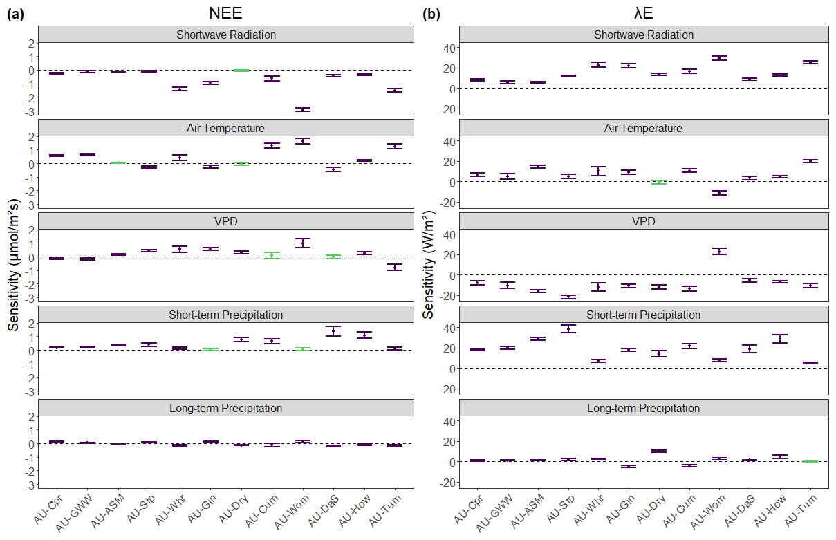
Figure 2Sensitivity of the flux to each climate variable for (a) NEE and (b) λE in the environmental memory models. Sites are on the x axis, ordered by ascending mean annual precipitation. The y axis is the sum of all Gn and Dn coefficients from Eq. (1), where n includes the climate variable, divided by the mean standard deviation of the corresponding weighted sums from Table 2, such that sensitivity values are comparable between variables. Where the range of sensitivity includes 0, those variables are considered to non-significantly affect the flux and are coloured green in the plots.
λE fluxes were sensitive to more climate variables than NEE fluxes. Across all sites and variables, only two climate drivers were not significant in their effect on λE at a site: air temperature at AU-Dry and long-term precipitation at AU-Tum. The lack of significance in long-term precipitation at AU-Tum may be due to this site being the wettest, with a MAP of over 1400 mm yr−1, and one of the sites with the most even rainfall distributions (CVP = 32). The driest year in the AU-Tum data is 2006, with 421 mm of precipitation, which is still greater than the MAP at the four driest sites in this study. Another result of interest is that the response of the λE flux to air temperature and VPD at AU-Wom was the opposite to the relationship at all other sites. AU-Wom exhibited an increase in λE with an increase in VPD and a decrease in the flux as temperature increased.
For both NEE and λE fluxes, there was a correlation between the sites' sensitivity to short-wave radiation and their wetness index (, p<0.05 for NEE; ρ=0.78, p<0.01 for λE). However when this relationship was explored by splitting between the two vegetation groups, it was only significant for the SAWS sites. The correlation was in fact stronger when only the woodland sites are considered ( and 0.86 for NEE and λE, respectively; p<0.05). When the NATT sites were taken in isolation, this relationship between site aridity and sensitivity to short-wave radiation was not apparent.
3.3 Timescales of memory influence
The cumulative weights from the EM model can provide evidence of the relevant timescales at which the significant climate variables affected NEE. These are shown for (a) air temperature and (b) long-term precipitation in Fig. 3. Following Liu et al. (2019), we assumed that the critical lag timescale is when the cumulative weight reached 0.5, indicated by the dashed line. For air temperature, at sites where this climate metric was significant, all but two sites had a lagged response of > 2 d. NEE at AU-Stp and AU-Gin had dependence on prior air temperature at longer timescales, around 4–5 d. The timescales at which precipitation affected NEE were much less consistent across sites. AU-DaS had a very short lag of only 21 d, while AU-Tum required over 270 d of prior rainfall to reach a weight of 0.5. The remaining sites had lags to long-term precipitation falling between these extremes but with no obvious correlation between MAP and response timescale. Similarly, there was no clear relationship between lagged response timescales and the prevalence of woody vegetation at the sites; both NATT and SAWS sites exhibited a range of critical timescales.

Figure 3Cumulative mean weights from the NEE EM model for (a) air temperature and (b) long-term precipitation. Sites are split into the (i) NATT and (ii) SAWS groups for each climate predictor. Within each group, sites are ordered by mean annual precipitation, with darker colours indicating higher MAP. Only sites where the climate variable is significant in Fig. 2a are included. The dashed line at a cumulative weight of 0.5 indicates the threshold for the critical lag period. Where the cumulative weights cross this line is considered the timescale of the environmental memory effect for each site for the climatic driver in question.
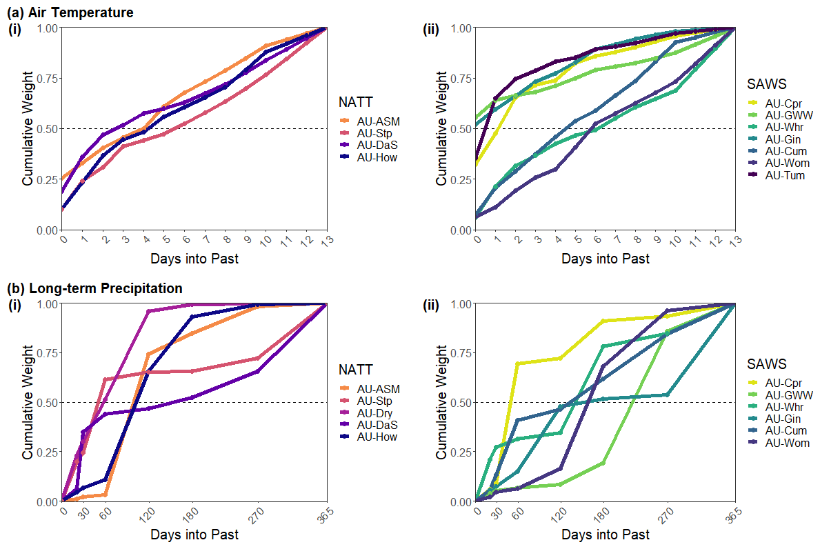
Figure 4Cumulative mean weights from the λE EM model for (a) air temperature and (b) long-term precipitation. Sites are split into the (i) NATT and (ii) SAWS groups for each climate predictor. Within each group, sites are ordered by mean annual precipitation, with darker colours indicating higher MAP. Only sites where the climate variable is significant in Fig. 2b are included. The dashed line at a cumulative weight of 0.5 indicates the threshold for the critical lag period. Where the cumulative weights cross this line is considered the timescale of the environmental memory effect for each site for the climatic driver in question.
Figure 4 shows that the timescale at which the λE flux responded to air temperature is generally longer than that for NEE. This may reflect the contribution of deep soil moisture (and so longer timescales) to transpiration fluxes (driven by VPD associated with higher temperature), whereas the impact of temperature on NEE, via for example heterotrophic respiration, would be controlled by shallower soil moisture (Parton et al., 1988). We found that 7 of the 12 sites responded to the air temperature from 3 to 7 d prior. Notably AU-Gin, which had a relatively long response timeframe for NEE to air temperature, had a strong immediate response for λE, with the critical timescale occurring at no lag. The shapes of the cumulative weight plots were more similar across sites for λE than for NEE, with a consistent increase across each lagged period and a much smaller range of initial weights calculated for the current air temperature.
For long-term precipitation, critical time periods for λE ranged from 60 to 270 d. No obvious relationship existed between site aridity and the timescales at which long-term precipitation affected evapotranspiration, indicating that other site characteristics (for example rooting depth) were influencing the lagged effects of rainfall. While the overall range of lagged responses to long-term precipitation was very similar between NEE and λE, the critical timescales for each flux differed at most sites (see Figs. 3b and 4b). For instance, at AU-Dry and AU-Stp, the critical lagged timescale for λE was 60 d, but for NEE a total lag of 270 d was required for a cumulative weight of over 0.5. Conversely, AU-DaS had a short lagged NEE response to long-term precipitation of 20 d, but the critical weight was reached at 180 d for λE.
3.4 Comparison to alternative modelling approaches
Finally, NEE fluxes were modelled using both an approach of k-means clustering plus regression and the CABLE TBM parameterised by PFT, the results of which are shown in Fig. 5. At every site, the EM SAM model performed better than a current-climate-only k-means model, which is to be expected due to the far greater degrees of freedom in the SAM models. The difference between the median k-means R2 and EM R2 ranges from 0.02 to 0.12. However, the introduction of the lags for individual climate variables to the k-means model generally improved performance, although the EM SAM model outperformed these models in most cases. When all lags were introduced to the k-means model, performance improved at all sites. Performance was comparable to or better than that of the EM SAM model, confirming the applicability of SAM for predicting terrestrial ecosystem fluxes.
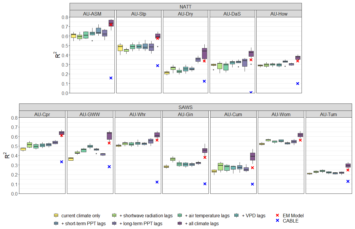
Figure 5R2 values for seven different models of k-means clustering plus regression predicting NEE at the flux sites, split by the two vegetation groups. “Current climate” is the k-means model that only considers concurrent environmental observations for predicting NEE. Each of the five lagged environmental predictors are then introduced separately; “+ all climate lags” is the model where every lagged environmental variable is included and hence utilises exactly the same predictors as the EM SAM model. Boxplots indicate the distribution of the R2 values when these models are run for between two and eight clusters each. The EM SAM model R2 value is indicated by a red cross, and the R2 for a PFT-parameterised TBM (CABLE) is shown with a blue cross. Note that AU-Wom had no available CABLE output. Sites are ordered from left to right by ascending mean annual precipitation within each vegetation group.
The sites were also modelled using the Australian TBM, the Community Atmosphere Biosphere Land Exchange model (CABLE). In these model runs, CABLE was parameterised by assumed PFT, with no site-specific calibration, and thus indicates a lower bound on TBM performance at the sites. As shown in Fig. 5, this consistently underperformed relative to the predictability expected from the empirical methods. R2 values for the TBM predictions against observed NEE ranged from 0 to 0.33, with a mean of 0.16. Performance was generally better at the SAWS sites than at the NATT sites. CABLE performed better as sites became drier within the SAWS group, but this behaviour was not seen for the NATT sites.
Prior to the introduction of the stochastic antecedent modelling framework (Ogle et al., 2015), little work had attempted to explicitly quantify the role and behaviour of these lagged effects. This paper provides further evidence that ecosystem fluxes exhibit complicated responses to antecedent conditions and that these responses are important components of ecosystem functioning and as such need to be further explored if these ecosystems are to be properly understood.
4.1 To what extent does environmental memory matter?
This study shows that understanding the lagged component in ecosystem responses to climate, that is the environmental memory, can significantly improve the ability to model site fluxes empirically. Introducing antecedent climate to the NEE model increased the R2 by an average of 0.08, which is a mean relative improvement of 22 % in model performance, with the relative improvement at individual sites ranging from 7 % to 55 %. For λE, the improvement ranged from 2 % to 49 %, with a mean of 20 %. This is reflective of the generally higher predictability of the λE flux compared to NEE, with more of the variance in the flux explained by current climate only. This improvement in model performance for both fluxes indicates that exploring the role of environmental memory could further substantially improve our understanding of site functioning.
While the EM model results provide a direct indication of the role of antecedent climate, we further modelled the flux residuals with an autoregressive lag-1 model (the AR model). The ensuing R2 value obtained was interpreted as a lower bound on overall site predictability based on prior conditions, contingent on the structural assumption of a lag of one time step. This is because the AR model captures remaining predictability from the previous day's fluxes without identifying the source of this influence. For instance, this dependence on prior-day flux may be affected by seasonal leaf area, delays between photosynthesis and respiration (Mencuccini and Hölttä, 2010), or potential site disturbances. It could also be representing environmental drivers that we have not explicitly accounted for, lagged allocation, or more unique impacts such as insect infestation.
Although eddy covariance analysis is a mature field, relatively little work has been done on quantifying environmental memory. Instead, the focus has been on immediate site responses to disturbance events and meteorological extremes (Ciais et al., 2005; von Buttlar et al., 2018; Teuling et al., 2010; Flach et al., 2018). At the site level, further examination of other controls on carbon and water fluxes (e.g. variability in leaf area, root zone soil moisture, the contribution of non-transpiration components, and the role of non-structural carbohydrates) may unlock explanations for why environmental memory varies both across the precipitation gradients and amongst similar geographic sites. For example, we found that our capacity to simulate NEE fluxes at AU-Cum was seemingly poorly explained by current climate. It is notable that Peters et al. (2021) recently highlighted the high tolerance of drought stress (xylem embolism resistance; p50: −4.07 to −5.82 MPa) of species at AU-Cum, which may explain an apparent decoupling between carbon fluxes and current meteorological conditions. Pinning down the exact mechanistic explanation will remain for future work, but our results motivate the search for hypotheses to explain differences in site behaviour. By characterising the extent of individual-site memory statistically, we hope to stimulate future site measurement campaigns and hypothesis development that examines what drives memory variability and ultimately guide model development. As for which TBM modules would need to be adjusted to fully capture environmental memory, this approach needs to be applied at many more individual sites. This would allow us to identify functional relationships to a greater extent. However, such application needs to be carefully pursued, using not just SAM but other machine learning approaches (such as the k-means clustering plus regression as we have demonstrated) to ensure that any results are process-based and not just structural assumptions from the use of a single modelling approach. By combining multiple empirical studies of environmental memory, we can understand the key lags that aid prediction of ecosystem fluxes and how these vary across site characteristics.
4.2 The benefits of stochastic antecedent modelling
Through the application of stochastic antecedent modelling, we have been able to identify the importance of environmental memory in ecosystem fluxes at a diverse range of Australian sites. Unlike traditional methods of exploring antecedent effects, SAM makes few prior assumptions about critical lag lengths beyond a prescribed maximum lag of interest (i.e. the 14 d window we assigned to the short-term variables). The Bayesian framework also yields the full (joint) posterior distribution for the parameters of interest, from which we can compute summaries such as credible intervals, allowing a critical assessment of the relative significance of various memory drivers. However, the SAM method is computationally intensive and requires long data records, which may reduce its potential applications. In this paper, we also perform similar analysis using the basic machine learning approach of k-means clustering plus regression. The results from the k-means modelling were broadly consistent with those from the SAM approach. Both modelling methodologies produced predictions with similar R2 values (Fig. 5) and saw improved performance when lagged climate effects were introduced. The k-means modelling in this study has provided a novel, independent check on the suitability and performance of the SAM approach. The consistent results increase our confidence in the findings from the SAM model and reduce the likelihood that our findings are influenced by the structural assumptions of the SAM model. Importantly, while computation of k means was significantly faster than SAM, the k-means approach lacks the inherent interpretability of SAM. While SAM is explicitly designed to infer the sensitivity to predictors and the timescales at which lags exist, the approach of k-means clustering plus regression would require further work and modelling to fully explore these aspects of flux responses, which is beyond the scope of this study. Since the k-means clustering plus regression often outperformed the SAM model, we have identified that the SAM approach does not provide an upper bound on the information available from the flux data. As such, our results highlight the need to explore the role of environmental memory using different approaches, including use of alternative machine learning techniques.
This study also showed how the relative influence of different drivers of NEE and λE fluxes can be discerned. By normalising the sensitivity parameters for each environmental driver, we further the work of Liu et al. (2019), allowing the individual climate predictors to be compared between variables and across sites. This increases the information provided by the SAM approach regarding the site behaviour and is a further argument for its use to explore the timescales of ecosystem response. Liu et al. (2019) provided a strong argument that including the influence of environmental memory is key for predicting ecosystem fluxes. Our results suggest that more careful site evaluation is likely to be required to truly understand the impact and source of these memory effects. Fortunately, the SAM approach, together with other machine learning techniques, is well positioned to provide the necessary insights to shine a new light on site dynamics and memory influence.
4.3 The importance of across-site heterogeneity
One of the key conclusions from Liu et al. (2019) was that as sites become more arid, the importance of antecedent effects increases. However, Liu et al. (2019) considered 42 sites from across the globe, incorporating a wide range of biomes and species. As such, there is potential for confounding factors to be influencing the importance of environmental memory at each site. This study reduces some of this uncertainty by limiting its scope to 12 sites, all located within Australia. This means that, as well as limiting the diversity of species and climates studied, a greater understanding of each individual site is possible. Similarly to Liu et al. (2019), these sites were grouped by biome, although we only had two groups: savannahs and grasslands within the NATT and woodlands in the SAWS group. Each biome group contains sites with a range of MAP and WI values. When these sites are viewed together, the importance of memory is strongly correlated with site aridity (improvement in R2 between CC and EM models; , p value <0.01), consistent with the conclusions of Liu et al. (2019). However, when the sites are split by our vegetation groupings, this significant correlation is only seen for the SAWS group (, p value <0.05), again noting that total sample size is reduced when we split by vegetation group. The NATT sites had no correlation between site memory and aridity (, p value =0.23), despite having a very strong rainfall gradient. Note that both groups have ranges of aridity that include sites spanning from “arid” to “humid”, with the WI at NATT sites between 0.12 and 0.75 and at SAWS sites between 0.11 and 1.2 (Trabucco and Zomer, 2018). This result indicates that grouping many sites together to explore relationships based on a single metric can obscure more nuanced understanding of the processes involved or the key site characteristics driving such relationships. For instance, at the savannah sites, we found that NEE sensitivity to short-term precipitation increases as site MAP increases. We hypothesise that this increased sensitivity is driven by the monsoonal nature of rainfall at the NATT sites with greater MAP. Our results also show that the relationship between short-wave radiation and site aridity is only seen in the SAWS grouping, not at the NATT sites. This is potentially due to the greater proportion of woody vegetation at SAWS sites, resulting in a greater rooting depth and less frequent water stress. As such, these sites are likely to be energy-limited, and hence transpiration is linked to days of high photosynthetically active radiation.
We have also found an inverse response of λE to temperature and VPD at AU-Wom to all other sites. It is not clear what the driver is here, and it is unlikely to be related to the correlation between temperature and VPD as this is higher at the other sites which did not exhibit this behaviour (ρ=0.85 at AU-Wom; five other sites have higher ρ values, up to 0.91). One possible cause is that AU-Wom generally has the lowest VPD observations across all sites, with only AU-Tum showing similar but greater values (median VPD = 0.20 kPa; other sites range from 0.31 to 1.94 kPa). While other sites may tend to close their stomata, limiting transpiration as VPD increases, AU-Wom is potentially below the VPD threshold at which stomata begin to limit transpiration. Similarly, Griebel et al. (2020) found that AU-Wom does not limit transpiration during hot temperatures and heatwaves, potentially due to access to deep water reserves. However, the inverse response could also be due to the vegetation composition at AU-Wom, with the potential for this effect to have been caused by photosynthetic inhibition at high temperatures (and high VPD), which would further explain why this opposite response is not seen in the NEE flux. The prevailing wind direction, which is seasonally dependent, heavily influences the flux tower footprint and affects the climate conditions at AU-Wom (Griebel et al., 2016). This could potentially contribute to the inverse behaviour seen if changes in VPD are correlated with significant changes in the vegetated area being measured by the tower. Additional exploration of the lags experienced at the AU-Wom site is probably necessary if this response is to be more precisely attributed.
Many studies have also highlighted how global relationships do not hold at regional, local, or even site level (Knapp and Smith, 2001; Knapp et al., 2017; Lauenroth and Sala, 1992; Ukkola et al., 2021; Wilcox et al., 2016). Such non-transferability is related to the issue of spatial versus temporal relationships and particularly the “vegetation structure constraint” (Lauenroth and Sala, 1992). This is where, due to the slow timescales at which species composition and plant function respond to changes in climate, individual sites are unable to fully utilise any inter-annual variability in climate conditions (Lauenroth and Sala, 1992). Here, we have shown that, within the range of Australian ecosystems analysed, environmental memory is not clearly related to site aridity for savannah sites. In comparison, among woodland sites, the link between environmental memory and site aridity appears to be stronger. Our results point to a need to better understand the role of individual-site characteristics (i.e. root zone water access) in determining predictability of carbon and water fluxes.
4.4 Implications for TBM evaluations
Flux data are routinely used to benchmark and improve TBM performance (Abramowitz, 2012; Abramowitz et al., 2008; Best et al., 2015; Haughton et al., 2016, 2018b; Nearing et al., 2018). In spite of this, relatively few studies have proposed that assessments of TBM performance at flux sites should also consider the underlying site predictability (but see Haughton et al., 2018a). Here, we argue that the confounding effect of baseline predictability is essential when comparing models that may have been tested at different sites and also in determining which ecosystems a model can best represent. Our results indicate that process-based TBMs tested at sites that exhibit greater predictability from simple empirical models, such as SAM or k means, as used in this paper, might be expected to perform better than TBMs tested at those sites which exhibit a lower baseline predictability of fluxes. For instance, Whitley et al. (2016) found that, when modelling gross primary productivity (GPP) and λE fluxes, the performance of a suite of TBMs improved slightly across the NATT sites as the MAP decreased. This is consistent with our findings of higher predictability at more arid sites. Importantly, this performance could be reinterpreted given the baseline predictability calculated using the SAM approach. Across the sites included in both this paper and Whitley et al. (2016), they found that model-averaged correlation coefficients for λE predictions had a maximum difference between sites of 0.08, ranging from 0.56 (AU-Dry) to 0.64 (AU-Stp). Our analysis found a similar difference between correlation coefficients of 0.06 (0.85 at AU-How and 0.91 at AU-Stp). This might show that both empirical models and TBMs perform better at drier sites. However, when we consider the TBM performance relative to the empirical SAM performance, AU-How actually performs better (TBMs capture 70 % of the expected predictability assumed from the SAM model) than the drier AU-Stp site (where TBMs capture 66 %).
Similarly, Barraza et al. (2017) modelled λE across the NATT using various indices of surface conductance and found that the sites with greater Eucalyptus occurrence (i.e. the wetter sites: AU-How, AU-DaS, and AU-Dry) were better represented by their model. However, if the reported R2 values from this study are considered relative to the values found in this study, then their models perform even better at the wet sites compared to the dry. The Eucalyptus-dominated sites have R2 values very similar to those from this study, while at AU-Stp and AU-ASM (the drier sites), the R2 values found in Barraza et al. (2017) are substantially lower.
Additionally, the CABLE model results in Fig. 5 illustrate how the results from empirical models can be used as a baseline for TBM performance. At AU-Cum, AU-Dry, AU-Gin, and AU-Whr, the R2 from CABLE is close to 0.1. However, from the SAM and k-means approaches, it is apparent that AU-Whr is more predictable than the other three sites. The performance of CABLE at AU-Whr is only around 18 % of the empirical models. At AU-Cum, the R2 of CABLE is approximately 25 % and 37 % of the R2 of k means and SAM, respectively. Hence, while initially CABLE appears to perform similarly well at both sites, it can be seen that the TBM is capturing more of the expected predictability at AU-Cum than at AU-Whr. As such, the baseline predictability of sites as calculated from detailed empirical models such as ours clearly provides a framework by which we can reinterpret the predictability of ecosystems and hence how well TBMs are performing.
Our results add to a growing body of research (for example, see Bastos et al., 2020; Ciais et al., 2005; Feldman et al., 2021; Liu et al., 2018; and Ogle et al., 2015) that identifies an important role of ecosystem “memory” in the terrestrial fluxes. This first step, including the characterisation of the timescale of influence, the processes affected (e.g. λE vs. NEE), the controlling environmental driver and site-to-site variability, is critical to improving TBMs. It is widely acknowledged that capturing legacy processes in TBMs is important (e.g. acclimation, recovery from climate extremes, link between carbon uptake and growth, canopy defoliation), but to develop the theory, we first need a strong evidence base against which we can probe model predictions. The challenge now is to link the statistical findings to mechanisms and then demonstrate that capturing these processes in models leads to improvements in site predictions. This second step will require applications of our approach (or similar) to both field and targeted experimental data, with progress likely to be made by linking directly to model–hypothesis testing (e.g. Katul et al., 2001; Mahecha et al., 2010).
Accurate prediction of carbon and water fluxes is key to understanding the role that terrestrial ecosystems will play in a changing climate. This study builds on previous work utilising stochastic antecedent modelling to provide further evidence that environmental memory is a key component of both net ecosystem exchange and latent heat fluxes. In general, the role of this memory effect increases as sites become more arid, yet we have shown that this relationship is confounded by individual-site characteristics and behaviour. By separating the influence of various predictors on NEE and λE fluxes, it becomes clear that despite this broad-scale relationship with aridity, very different mechanisms are at play across sites. The differences we report in site behaviour should motivate a range of new hypotheses in future research to understand the controls on variability in predictability of site fluxes. Finally, we argue that a consideration of both site predictability and environmental memory should form a key part of terrestrial biosphere model evaluation and future process development.
OzFlux data are available from https://www.ozflux.org.au/ (OzFlux Australian and New Zealand Flux Research and Monitoring, 2021). Model codes, example workflows, and select analysis scripts are available at https://doi.org/10.5281/zenodo.6361060 (Cranko Page et al., 2022) and https://github.com/JDCP93/OzFlux_SAM.
The supplement related to this article is available online at: https://doi.org/10.5194/bg-19-1913-2022-supplement.
JCP performed all model runs and code analysis, with input from MGDK, GA, YL, and KO. JCP wrote the manuscript with substantial input from MGDK, GA, MJH, JC, YL, and KO. AJP and NHN provided further input on the manuscript.
At least one of the (co-)authors is a member of the editorial board of Biogeosciences. The peer-review process was guided by an independent editor, and the authors also have no other competing interests to declare.
Publisher’s note: Copernicus Publications remains neutral with regard to jurisdictional claims in published maps and institutional affiliations.
Jon Cranko Page, Martin G. De Kauwe, Gab Abramowitz, and Andy J. Pitman were supported by the Australian Research Council Centre of Excellence for Climate Extremes (CE170100023). Mark J. Hovenden , Martin G. De Kauwe, and Kiona Ogle were supported by the ARC Discovery Grant (grant no. DP190102025). Martin G. De Kauwe received additional support from the ARC Discovery Grant (grant no. DP190101823) and the NSW Research Attraction and Acceleration Program.
This paper was edited by Alexandra Konings and reviewed by two anonymous referees.
Abramowitz, G.: Towards a public, standardized, diagnostic benchmarking system for land surface models, Geosci. Model Dev., 5, 819–827, https://doi.org/10.5194/gmd-5-819-2012, 2012. a, b
Abramowitz, G., Pitman, A., Gupta, H., Kowalczyk, E., and Wang, Y.: Systematic Bias in Land Surface Models, J. Hydrometeorol., 8, 989–1001, https://doi.org/10.1175/JHM628.1, 2007. a
Abramowitz, G., Leuning, R., Clark, M., and Pitman, A.: Evaluating the Performance of Land Surface Models, J. Clim., 21, 5468–5481, https://doi.org/10.1175/2008JCLI2378.1, 2008. a
Anderegg, W. R. L., Schwalm, C., Biondi, F., Camarero, J. J., Koch, G., Litvak, M., Ogle, K., Shaw, J. D., Shevliakova, E., Williams, A. P., Wolf, A., Ziaco, E., and Pacala, S.: Pervasive Drought Legacies in Forest Ecosystems and Their Implications for Carbon Cycle Models, Science, 349, 528–532, https://doi.org/10.1126/science.aab1833, 2015. a, b, c, d
Arndt, S., Hinko-Najera, N., and Griebel, A.: Wombat Wombat State Forest Flux Data Collection Level 6, Terrestrial Ecosystem Research Network (TERN) [data set], https://hdl.handle.net/102.100.100/14237 (last access: 21 September 2021), 2013. a
Barraza, V., Restrepo-Coupe, N., Huete, A., Grings, F., Beringer, J., Cleverly, J., and Eamus, D.: Estimation of Latent Heat Flux over Savannah Vegetation across the North Australian Tropical Transect from Multiple Sensors and Global Meteorological Data, Agr. Forest Meteorol., 232, 689–703, https://doi.org/10.1016/j.agrformet.2016.10.013, 2017. a, b
Barron-Gafford, G. A., Cable, J. M., Bentley, L. P., Scott, R. L., Huxman, T. E., Jenerette, G. D., and Ogle, K.: Quantifying the Timescales over Which Exogenous and Endogenous Conditions Affect Soil Respiration, New Phytol., 202, 442–454, https://doi.org/10.1111/nph.12675, 2014. a
Bastos, A., Ciais, P., Friedlingstein, P., Sitch, S., Pongratz, J., Fan, L., Wigneron, J. P., Weber, U., Reichstein, M., Fu, Z., Anthoni, P., Arneth, A., Haverd, V., Jain, A. K., Joetzjer, E., Knauer, J., Lienert, S., Loughran, T., McGuire, P. C., Tian, H., Viovy, N., and Zaehle, S.: Direct and Seasonal Legacy Effects of the 2018 Heat Wave and Drought on European Ecosystem Productivity, Sci. Adv., 6, eaba2724, https://doi.org/10.1126/sciadv.aba2724, 2020. a
Beringer, J., Hutley, L., and Northwood, M.: Daly Daly Uncleared Flux Data Collection Level 6, Terrestrial Ecosystem Research Network (TERN) [data set], https://hdl.handle.net/102.100.100/14239 (last access: 21 September 2021), 2015a. a
Beringer, J., Hutley, L., and Northwood, M.: Dry River Flux Data Collection Level 6, Terrestrial Ecosystem Research Network (TERN) [data set], https://hdl.handle.net/102.100.100/14229 (last access: 21 September 2021), 2015b. a
Beringer, J., Hutley, L., and Northwood, M.: Howard Springs Flux Data Collection Level 6, Terrestrial Ecosystem Research Network (TERN) [data set], https://hdl.handle.net/102.100.100/14234 (last access: 21 September 2021), 2015c. a
Beringer, J., Hutley, L., and Northwood, M.: Sturt Plains Flux Data Collection Level 6, Terrestrial Ecosystem Research Network (TERN) [data set], https://hdl.handle.net/102.100.100/14230 (last access: 21 September 2021), 2015d. a
Beringer, J., Hutley, L., Hinko-Najera, N., and McHugh, I.: Whroo Flux Data Collection Level 6, Terrestrial Ecosystem Research Network (TERN) [data set], https://hdl.handle.net/102.100.100/14232 (last access: 21 September 2021), 2017. a
Beringer, J., Hutley, L. B., McHugh, I., Arndt, S. K., Campbell, D., Cleugh, H. A., Cleverly, J., Resco de Dios, V., Eamus, D., Evans, B., Ewenz, C., Grace, P., Griebel, A., Haverd, V., Hinko-Najera, N., Huete, A., Isaac, P., Kanniah, K., Leuning, R., Liddell, M. J., Macfarlane, C., Meyer, W., Moore, C., Pendall, E., Phillips, A., Phillips, R. L., Prober, S. M., Restrepo-Coupe, N., Rutledge, S., Schroder, I., Silberstein, R., Southall, P., Yee, M. S., Tapper, N. J., van Gorsel, E., Vote, C., Walker, J., and Wardlaw, T.: An introduction to the Australian and New Zealand flux tower network – OzFlux, Biogeosciences, 13, 5895–5916, https://doi.org/10.5194/bg-13-5895-2016, 2016. a
Best, M. J., Abramowitz, G., Johnson, H. R., Pitman, A. J., Balsamo, G., Boone, A., Cuntz, M., Decharme, B., Dirmeyer, P. A., Dong, J., Ek, M., Guo, Z., Haverd, V., van den Hurk, B. J. J., Nearing, G. S., Pak, B., Peters-Lidard, C., Santanello, J. A., Stevens, L., and Vuichard, N.: The Plumbing of Land Surface Models: Benchmarking Model Performance, J. Hydrometeorol., 16, 1425–1442, https://doi.org/10.1175/JHM-D-14-0158.1, 2015. a, b, c
Cable, J. M., Ogle, K., Barron-Gafford, G. A., Bentley, L. P., Cable, W. L., Scott, R. L., Williams, D. G., and Huxman, T. E.: Antecedent Conditions Influence Soil Respiration Differences in Shrub and Grass Patches, Ecosystems, 16, 1230–1247, https://doi.org/10.1007/s10021-013-9679-7, 2013. a, b, c
Charrad, M., Ghazzali, N., Boiteau, V., and Niknafs, A.: NbClust: An R Package for Determining the Relevant Number of Clusters in a Data Set, J. Stat. Softw., 61, 1–36, https://doi.org/10.18637/jss.v061.i06, 2014. a
Ciais, P., Reichstein, M., Viovy, N., Granier, A., Ogée, J., Allard, V., Aubinet, M., Buchmann, N., Bernhofer, C., Carrara, A., Chevallier, F., De Noblet, N., Friend, A. D., Friedlingstein, P., Grünwald, T., Heinesch, B., Keronen, P., Knohl, A., Krinner, G., Loustau, D., Manca, G., Matteucci, G., Miglietta, F., Ourcival, J. M., Papale, D., Pilegaard, K., Rambal, S., Seufert, G., Soussana, J. F., Sanz, M. J., Schulze, E. D., Vesala, T., and Valentini, R.: Europe-Wide Reduction in Primary Productivity Caused by the Heat and Drought in 2003, Nature, 437, 529–533, https://doi.org/10.1038/nature03972, 2005. a, b
Cleverly, J., Eamus, D., Faux, R., Grant, N., and Li, Z.: Alice Springs Mulga Flux Data Collection Level 5, Terrestrial Ecosystem Research Network (TERN) [data set], https://hdl.handle.net/102.100.100/14217 (last access: 21 September 2021), 2015. a
Cleverly, J., Boulain, N., Villalobos-Vega, R., Grant, N., Faux, R., Wood, C., Cook, P. G., Yu, Q., Leigh, A., and Eamus, D.: Dynamics of Component Carbon Fluxes in a Semi-Arid Acacia Woodland, Central Australia, J. Geophys. Res.-Biogeosci., 118, 1168–1185, https://doi.org/10.1002/jgrg.20101, 2013. a
Cleverly, J., Eamus, D., Restrepo Coupe, N., Chen, C., Maes, W., Li, L., Faux, R., Santini, N. S., Rumman, R., Yu, Q., and Huete, A.: Soil Moisture Controls on Phenology and Productivity in a Semi-Arid Critical Zone, Sci. Total Environ., 568, 1227–1237, https://doi.org/10.1016/j.scitotenv.2016.05.142, 2016. a
Cranko Page, J., De Kauwe, M. G., Abramowitz, G., Liu, Y., and Ogle, K.: OzFlux_SAM, Zenodo [code], https://doi.org/10.5281/zenodo.6361060, 2022. a
De Kauwe, M. G., Kala, J., Lin, Y.-S., Pitman, A. J., Medlyn, B. E., Duursma, R. A., Abramowitz, G., Wang, Y.-P., and Miralles, D. G.: A test of an optimal stomatal conductance scheme within the CABLE land surface model, Geosci. Model Dev., 8, 431–452, https://doi.org/10.5194/gmd-8-431-2015, 2015a. a
De Kauwe, M. G., Zhou, S.-X., Medlyn, B. E., Pitman, A. J., Wang, Y.-P., Duursma, R. A., and Prentice, I. C.: Do land surface models need to include differential plant species responses to drought? Examining model predictions across a mesic-xeric gradient in Europe, Biogeosciences, 12, 7503–7518, https://doi.org/10.5194/bg-12-7503-2015, 2015b. a
Decker, M., Or, D., Pitman, A., and Ukkola, A.: New Turbulent Resistance Parameterization for Soil Evaporation Based on a Pore-Scale Model: Impact on Surface Fluxes in CABLE, J. Adv. Model. Earth Syst., 9, 220–238, https://doi.org/10.1002/2016MS000832, 2017. a
Fanjul, L. and Jones, H. G.: Rapid Stomatal Responses to Humidity, Planta, 154, 135–138, https://doi.org/10.1007/BF00387906, 1982. a
Fatichi, S., Leuzinger, S., and Körner, C.: Moving beyond Photosynthesis: From Carbon Source to Sink-Driven Vegetation Modeling, New Phytol., 201, 1086–1095, https://doi.org/10.1111/nph.12614, 2014. a
Feldman, A. F., Short Gianotti, D. J., Konings, A. G., Gentine, P., and Entekhabi, D.: Patterns of plant rehydration and growth following pulses of soil moisture availability, Biogeosciences, 18, 831–847, https://doi.org/10.5194/bg-18-831-2021, 2021. a, b
Fick, S. E. and Hijmans, R. J.: WorldClim 2: New 1-Km Spatial Resolution Climate Surfaces for Global Land Areas, Int. J. Climatol., 37, 4302–4315, https://doi.org/10.1002/joc.5086, 2017. a, b
Flach, M., Sippel, S., Gans, F., Bastos, A., Brenning, A., Reichstein, M., and Mahecha, M. D.: Contrasting biosphere responses to hydrometeorological extremes: revisiting the 2010 western Russian heatwave, Biogeosciences, 15, 6067–6085, https://doi.org/10.5194/bg-15-6067-2018, 2018. a
Frank, D., Reichstein, M., Bahn, M., Thonicke, K., Frank, D., Mahecha, M. D., Smith, P., van der Velde, M., Vicca, S., Babst, F., Beer, C., Buchmann, N., Canadell, J. G., Ciais, P., Cramer, W., Ibrom, A., Miglietta, F., Poulter, B., Rammig, A., Seneviratne, S. I., Walz, A., Wattenbach, M., Zavala, M. A., and Zscheischler, J.: Effects of Climate Extremes on the Terrestrial Carbon Cycle: Concepts, Processes and Potential Future Impacts, Glob. Change Biol., 21, 2861–2880, https://doi.org/10.1111/gcb.12916, 2015. a
Gorelick, N., Hancher, M., Dixon, M., Ilyushchenko, S., Thau, D., and Moore, R.: Google Earth Engine: Planetary-scale Geospatial Analysis for Everyone, Remote Sens. Environ., 202, 18–27, https://doi.org/10.1016/j.rse.2017.06.031, 2017. a
Griebel, A., Bennett, L. T., Metzen, D., Cleverly, J., Burba, G., and Arndt, S. K.: Effects of Inhomogeneities within the Flux Footprint on the Interpretation of Seasonal, Annual, and Interannual Ecosystem Carbon Exchange, Agr. Forest Meteorol., 221, 50–60, https://doi.org/10.1016/j.agrformet.2016.02.002, 2016. a
Griebel, A., Bennett, L. T., Metzen, D., Pendall, E., Lane, P. N. J., and Arndt, S. K.: Trading Water for Carbon: Maintaining Photosynthesis at the Cost of Increased Water Loss During High Temperatures in a Temperate Forest, J. Geophys. Res.-Biogeosci., 125, e2019JG005239, https://doi.org/10.1029/2019JG005239, 2020. a
Harms, R. L. and Roebroeck, A.: Robust and Fast Markov Chain Monte Carlo Sampling of Diffusion MRI Microstructure Models, Front. Neuroinformatics, 12, 97, https://doi.org/10.3389/fninf.2018.00097, 2018. a
Haughton, N., Abramowitz, G., Pitman, A. J., Or, D., Best, M. J., Johnson, H. R., Balsamo, G., Boone, A., Cuntz, M., Decharme, B., Dirmeyer, P. A., Dong, J., Ek, M., Guo, Z., Haverd, V., van den Hurk, B. J. J., Nearing, G. S., Pak, B., Santanello, J. A., Stevens, L. E., and Vuichard, N.: The Plumbing of Land Surface Models: Is Poor Performance a Result of Methodology or Data Quality?, J. Hydrometeorol., 17, 1705–1723, https://doi.org/10.1175/JHM-D-15-0171.1, 2016. a, b, c
Haughton, N., Abramowitz, G., De Kauwe, M. G., and Pitman, A. J.: Does predictability of fluxes vary between FLUXNET sites?, Biogeosciences, 15, 4495–4513, https://doi.org/10.5194/bg-15-4495-2018, 2018a. a
Haughton, N., Abramowitz, G., and Pitman, A. J.: On the predictability of land surface fluxes from meteorological variables, Geosci. Model Dev., 11, 195–212, https://doi.org/10.5194/gmd-11-195-2018, 2018b. a
Haverd, V., Smith, B., Nieradzik, L. P., and Briggs, P. R.: A stand-alone tree demography and landscape structure module for Earth system models: integration with inventory data from temperate and boreal forests, Biogeosciences, 11, 4039–4055, https://doi.org/10.5194/bg-11-4039-2014, 2014. a
Haverd, V., Smith, B., Nieradzik, L., Briggs, P. R., Woodgate, W., Trudinger, C. M., Canadell, J. G., and Cuntz, M.: A new version of the CABLE land surface model (Subversion revision r4601) incorporating land use and land cover change, woody vegetation demography, and a novel optimisation-based approach to plant coordination of photosynthesis, Geosci. Model Dev., 11, 2995–3026, https://doi.org/10.5194/gmd-11-2995-2018, 2018. a
Hovenden, M. J., Newton, P. C. D., and Wills, K. E.: Seasonal Not Annual Rainfall Determines Grassland Biomass Response to Carbon Dioxide, Nature, 511, 583–586, https://doi.org/10.1038/nature13281, 2014. a
Hovenden, M. J., Newton, P. C. D., and Newton, P. C. D.: Variability in Precipitation Seasonality Limits Grassland Biomass Responses to Rising CO2: Historical and Projected Climate Analyses, Climatic Change; Dordrecht, Climatic Change, 149, 219–231, https://doi.org/10.1007/s10584-018-2227-x, 2018. a
Huang, Y., Gerber, S., Huang, T., and Lichstein, J. W.: Evaluating the Drought Response of CMIP5 Models Using Global Gross Primary Productivity, Leaf Area, Precipitation, and Soil Moisture Data, Global Biogeochem. Cy., 30, 1827–1846, https://doi.org/10.1002/2016GB005480, 2016. a
Humphrey, V., Zscheischler, J., Ciais, P., Gudmundsson, L., Sitch, S., and Seneviratne, S. I.: Sensitivity of Atmospheric CO 2 Growth Rate to Observed Changes in Terrestrial Water Storage, Nature, 560, 628–631, https://doi.org/10.1038/s41586-018-0424-4, 2018. a
Hutley, L. B., Beringer, J., Isaac, P. R., Hacker, J. M., and Cernusak, L. A.: A Sub-Continental Scale Living Laboratory: Spatial Patterns of Savanna Vegetation over a Rainfall Gradient in Northern Australia, Agr. Forest Meteorol., 151, 1417–1428, https://doi.org/10.1016/j.agrformet.2011.03.002, 2011. a
Huxman, T. E., Snyder, K. A., Tissue, D., Leffler, A. J., Ogle, K., Pockman, W. T., Sandquist, D. R., Potts, D. L., and Schwinning, S.: Precipitation Pulses and Carbon Fluxes in Semiarid and Arid Ecosystems, Oecologia, 141, 254–268, https://doi.org/10.1007/s00442-004-1682-4, 2004. a
Isaac, P., Cleverly, J., McHugh, I., van Gorsel, E., Ewenz, C., and Beringer, J.: OzFlux data: network integration from collection to curation, Biogeosciences, 14, 2903–2928, https://doi.org/10.5194/bg-14-2903-2017, 2017. a
Jones, S., Rowland, L., Cox, P., Hemming, D., Wiltshire, A., Williams, K., Parazoo, N. C., Liu, J., da Costa, A. C. L., Meir, P., Mencuccini, M., and Harper, A. B.: The impact of a simple representation of non-structural carbohydrates on the simulated response of tropical forests to drought, Biogeosciences, 17, 3589–3612, https://doi.org/10.5194/bg-17-3589-2020, 2020. a
Kannenberg, S. A., Schwalm, C. R., and Anderegg, W. R. L.: Ghosts of the Past: How Drought Legacy Effects Shape Forest Functioning and Carbon Cycling, Ecol. Lett., 23, 891–901, https://doi.org/10.1111/ele.13485, 2020. a, b
Katul, G., Lai, C.-T., Schäfer, K., Vidakovic, B., Albertson, J., Ellsworth, D., and Oren, R.: Multiscale Analysis of Vegetation Surface Fluxes: From Seconds to Years, Adv. Water Resour., 24, 1119–1132, https://doi.org/10.1016/S0309-1708(01)00029-X, 2001. a
Keenan, T., Baker, I., Barr, A., Ciais, P., Davis, K., Dietze, M., Dragoni, D., Gough, C. M., Grant, R., Hollinger, D., Hufkens, K., Poulter, B., McCaughey, H., Raczka, B., Ryu, Y., Schaefer, K., Tian, H., Verbeeck, H., Zhao, M., and Richardson, A. D.: Terrestrial Biosphere Model Performance for Inter-Annual Variability of Land-Atmosphere CO2 Exchange, Glob. Change Biol., 18, 1971–1987, https://doi.org/10.1111/j.1365-2486.2012.02678.x, 2012. a
Knapp, A. K. and Smith, M. D.: Variation among Biomes in Temporal Dynamics of Aboveground Primary Production, Science, 291, 481–484, 2001. a
Knapp, A. K., Ciais, P., and Smith, M. D.: Reconciling Inconsistencies in Precipitation – Productivity Relationships: Implications for Climate Change, New Phytol., 214, 41–47, https://doi.org/10.1111/nph.14381, 2017. a
Knight, J.: Root Distributions and Water Uptake Patterns in Eucalypts and Other Species, The ways trees use water, Rural Industries Research and Development Corporation, pp. 66–93, ISBN 0-642-57811-7, 1999. a
Kolus, H. R., Huntzinger, D. N., Schwalm, C. R., Fisher, J. B., McKay, N., Fang, Y., Michalak, A. M., Schaefer, K., Wei, Y., Poulter, B., Mao, J., Parazoo, N. C., and Shi, X.: Land Carbon Models Underestimate the Severity and Duration of Drought's Impact on Plant Productivity, Sci. Rep., 9, 2758, https://doi.org/10.1038/s41598-019-39373-1, 2019. a
Kowalczyk, E., Wang, Y., Law, R., Davies, H., Mcgregor, J., and Abramowitz, G.: The CSIRO Atmosphere Biosphere Land Exchange (CABLE) Model for Use in Climate Models and as an Offline Model, CSIRO Mar. Atmos. Res., 13, 1615, https://doi.org/10.4225/08/58615c6a9a51d, 2006. a
Kowalczyk, E., Stevens, L., Law, R., Dix, M., Wang, Y., Harman, I., Haynes, K., Srbinovsky, J., Pak, B., and Ziehn, T.: The Land Surface Model Component of ACCESS: Description and Impact on the Simulated Surface Climatology, Aust. Meteorol. Oceanogr. J., 63, 65–82, https://doi.org/10.22499/2.6301.005, 2013. a
Kruschke, J. K.: Doing Bayesian Data Analysis: A Tutorial with R, JAGS, and Stan, Academic Press, Boston, edition 2 edn., 143–191, ISBN 978-0-12-405888-0, 2015. a
Lasslop, G., Reichstein, M., Kattge, J., and Papale, D.: Influences of Observation Errors in Eddy Flux Data on Inverse Model Parameter Estimation, Biogeosciences, 5, 1311–1324, https://doi.org/10.5194/bg-5-1311-2008, 2008. a
Lauenroth, W. K. and Sala, O. E.: Long-Term Forage Production of North American Shortgrass Steppe, Ecol. Appl., 2, 397–403, https://doi.org/10.2307/1941874, 1992. a, b, c
Lemoine, N. P., Griffin-Nolan, R. J., Lock, A. D., and Knapp, A. K.: Drought Timing, Not Previous Drought Exposure, Determines Sensitivity of Two Shortgrass Species to Water Stress, Oecologia, 188, 965–975, https://doi.org/10.1007/s00442-018-4265-5, 2018. a
Liu, L., Zhang, Y., Wu, S., Li, S., and Qin, D.: Water Memory Effects and Their Impacts on Global Vegetation Productivity and Resilience, Sci. Rep., 8, 2962, https://doi.org/10.1038/s41598-018-21339-4, 2018. a, b
Liu, Y., Schwalm, C. R., Samuels-Crow, K. E., and Ogle, K.: Ecological Memory of Daily Carbon Exchange across the Globe and Its Importance in Drylands, Ecol. Lett., 22, 1806–1816, https://doi.org/10.1111/ele.13363, 2019. a, b, c, d, e, f, g, h, i, j, k, l, m
Lorenz, R., Pitman, A. J., Donat, M. G., Hirsch, A. L., Kala, J., Kowalczyk, E. A., Law, R. M., and Srbinovsky, J.: Representation of climate extreme indices in the ACCESS1.3b coupled atmosphere–land surface model, Geosci. Model Dev., 7, 545–567, https://doi.org/10.5194/gmd-7-545-2014, 2014. a
Macfarlane, C., Prober, S., and Wiehl, G.: Great Western Woodlands Flux Data Collection Level 6, Terrestrial Ecosystem Research Network (TERN) [data set], https://hdl.handle.net/102.100.100/14226 (last access: 21 September 2021), 2013. a
Mahecha, M. D., Reichstein, M., Jung, M., Seneviratne, S. I., Zaehle, S., Beer, C., Braakhekke, M. C., Carvalhais, N., Lange, H., Le Maire, G., and Moors, E.: Comparing Observations and Process-Based Simulations of Biosphere-Atmosphere Exchanges on Multiple Timescales, J. Geophys. Res.-Biogeosci., 115, G02003, https://doi.org/10.1029/2009JG001016, 2010. a
Mencuccini, M. and Hölttä, T.: The Significance of Phloem Transport for the Speed with Which Canopy Photosynthesis and Belowground Respiration Are Linked, New Phytol., 185, 189–203, https://doi.org/10.1111/j.1469-8137.2009.03050.x, 2010. a
Meyer, W., Ewenz, C., Koerber, G., and Lubcke, T.: Calperum Flux Data Collection Level 6, Terrestrial Ecosystem Research Network (TERN) [data set], https://hdl.handle.net/102.100.100/14236 (last access: 21 September 2021), 2013. a
Mottl, O., Flantua, S. G. A., Bhatta, K. P., Felde, V. A., Giesecke, T., Goring, S., Grimm, E. C., Haberle, S., Hooghiemstra, H., Ivory, S., Kuneš, P., Wolters, S., Seddon, A. W. R., and Williams, J. W.: Global Acceleration in Rates of Vegetation Change over the Past 18,000 Years, Science, 372, 860–864, https://doi.org/10.1126/science.abg1685, 2021. a
Nearing, G. S., Ruddell, B. L., Clark, M. P., Nijssen, B., and Peters-Lidard, C.: Benchmarking and Process Diagnostics of Land Models, J. Hydrometeorol., 19, 1835–1852, https://doi.org/10.1175/JHM-D-17-0209.1, 2018. a
Ogle, K. and Barber, J. J.: Plant and Ecosystem Memory, CHANCE, 29, 16–22, https://doi.org/10.1080/09332480.2016.1181961, 2016. a
Ogle, K., Barber, J. J., Barron-Gafford, G. A., Bentley, L. P., Young, J. M., Huxman, T. E., Loik, M. E., and Tissue, D. T.: Quantifying Ecological Memory in Plant and Ecosystem Processes, Ecol. Lett., 18, 221–235, https://doi.org/10.1111/ele.12399, 2015. a, b, c
Olson, D. M., Dinerstein, E., Wikramanayake, E. D., Burgess, N. D., Powell, G. V. N., Underwood, E. C., D'amico, J. A., Itoua, I., Strand, H. E., Morrison, J. C., Loucks, C. J., Allnutt, T. F., Ricketts, T. H., Kura, Y., Lamoreux, J. F., Wettengel, W. W., Hedao, P., and Kassem, K. R.: Terrestrial Ecoregions of the World: A New Map of Life on Earth: A New Global Map of Terrestrial Ecoregions Provides an Innovative Tool for Conserving Biodiversity, BioScience, 51, 933–938, https://doi.org/10.1641/0006-3568(2001)051[0933:TEOTWA]2.0.CO;2, 2001. a
OzFlux Australian and New Zealand Flux Research and Monitoring: https://www.ozflux.org.au/ (last access: 21 September 2021), 2021. a
Parton, W. J., Stewart, J. W. B., and Cole, C. V.: Dynamics of C, N, P and S in Grassland Soils: A Model, Biogeochemistry, 5, 109–131, https://doi.org/10.1007/BF02180320, 1988. a
Pendall, E., Griebel, A., and Barton, C., and Metzen, D.: Cumberland Plain Flux Data Collection Level 6, Terrestrial Ecosystem Research Network (TERN) [data set], https://hdl.handle.net/102.100.100/25164 (last access: 21 September 2021), 2019. a
Peters, J. M. R., López, R., Nolf, M., Hutley, L. B., Wardlaw, T., Cernusak, L. A., and Choat, B.: Living on the Edge: A Continental-Scale Assessment of Forest Vulnerability to Drought, Glob. Change Biol., 27, 3620–3641, https://doi.org/10.1111/gcb.15641, 2021. a
Pitman, A. J., Avila, F. B., Abramowitz, G., Wang, Y. P., Phipps, S. J., and de Noblet-Ducoudré, N.: Importance of Background Climate in Determining Impact of Land-Cover Change on Regional Climate, Nat. Clim. Change, 1, 472–475, https://doi.org/10.1038/nclimate1294, 2011. a
Plummer, M.: JAGS: A Program for Analysis of Bayesian Graphical Models Using Gibbs Sampling, 3rd International Workshop on Distributed Statistical Computing (DSC 2003); Vienna, Austria, 124, 2003. a
Plummer, M., Best, N., Cowles, K., and Vines, K.: CODA: Convergence Diagnosis and Output Analysis for MCMC, R News, 6, 7–11, 2006. a
R Core Team: R: A Language and Environment for Statistical Computing, R Foundation for Statistical Computing, 2020. a
Raupach, M. R.: Simplified Expressions for Vegetation Roughness Length and Zero-Plane Displacement as Functions of Canopy Height and Area Index, Bound.-Lay. Meteorol., 71, 211–216, https://doi.org/10.1007/BF00709229, 1994. a
Raupach, M. R., Finkele, K., and Zhang, L.: SCAM: A Soil-Canopy-Atmosphere Model: Description and Comparisons with Field Data, Technical Report 132, CSIRO Centre for Environmental Mechanics, Canberra, ACT, Australia, 1997. a
Renchon, A. A., Drake, J. E., Macdonald, C. A., Sihi, D., Hinko-Najera, N., Tjoelker, M. G., Arndt, S. K., Noh, N. J., Davidson, E., and Pendall, E.: Concurrent Measurements of Soil and Ecosystem Respiration in a Mature Eucalypt Woodland: Advantages, Lessons, and Questions, J. Geophys. Res.-Biogeosci., 126, e2020JG006221, https://doi.org/10.1029/2020JG006221, 2021. a
Richardson, A. D., Hollinger, D. Y., Burba, G. G., Davis, K. J., Flanagan, L. B., Katul, G. G., William Munger, J., Ricciuto, D. M., Stoy, P. C., Suyker, A. E., Verma, S. B., and Wofsy, S. C.: A Multi-Site Analysis of Random Error in Tower-Based Measurements of Carbon and Energy Fluxes, Agr. Forest Meteorol., 136, 1–18, https://doi.org/10.1016/j.agrformet.2006.01.007, 2006. a
Ryan, E. M., Ogle, K., Zelikova, T. J., LeCain, D. R., Williams, D. G., Morgan, J. A., and Pendall, E.: Antecedent Moisture and Temperature Conditions Modulate the Response of Ecosystem Respiration to Elevated CO2 and Warming, Glob. Change Biol., 21, 2588–2602, https://doi.org/10.1111/gcb.12910, 2015. a
Ryan, E. M., Ogle, K., Peltier, D., Walker, A. P., De Kauwe, M. G., Medlyn, B. E., Williams, D. G., Parton, W., Asao, S., Guenet, B., Harper, A. B., Lu, X., Luus, K. A., Zaehle, S., Shu, S., Werner, C., Xia, J., and Pendall, E.: Gross Primary Production Responses to Warming, Elevated CO2, and Irrigation: Quantifying the Drivers of Ecosystem Physiology in a Semiarid Grassland, Glob. Change Biol., 23, 3092–3106, https://doi.org/10.1111/gcb.13602, 2017. a, b
Sala, O. E., Gherardi, L. A., Reichmann, L., Jobbágy, E., and Peters, D.: Legacies of Precipitation Fluctuations on Primary Production: Theory and Data Synthesis, Philos. T. Roy. Soc. B, 367, 3135–3144, https://doi.org/10.1098/rstb.2011.0347, 2012. a, b
Samuels-Crow, K. E., Ogle, K., and Litvak, M. E.: Atmosphere-Soil Interactions Govern Ecosystem Flux Sensitivity to Environmental Conditions in Semiarid Woody Ecosystems Over Varying Timescales, J. Geophys. Res.-Biogeosci., 125, e2019JG005554, https://doi.org/10.1029/2019JG005554, 2020. a
Schaaf, C. and Wang, Z.: MCD43A3 MODIS/Terra+Aqua BRDF/Albedo Daily L3 Global – 500m V006, NASA EOSDIS Land Processes DAAC, https://doi.org/10.5067/MODIS/MCD43A3.006, 2015. a
Seabloom, E. W., Borer, E. T., and Tilman, D.: Grassland Ecosystem Recovery after Soil Disturbance Depends on Nutrient Supply Rate, Ecol. Lett., 23, ele.13591, https://doi.org/10.1111/ele.13591, 2020. a
Silberstein, R., Lambert, P., Lardner, T., and Macfarlane, C.: Gingin Flux Data Collection Level 6, Terrestrial Ecosystem Research Network (TERN) [data set], https://hdl.handle.net/102.100.100/22677 (last access: 21 September 2021), 2015. a
Smith, N. G. and Dukes, J. S.: Plant Respiration and Photosynthesis in Global-Scale Models: Incorporating Acclimation to Temperature and CO2, Glob. Change Biol., 19, 45–63, https://doi.org/10.1111/j.1365-2486.2012.02797.x, 2013. a
Stoll, J. and Kitchen, M.: Tumbarumba Flux Data Collection Level 6, Terrestrial Ecosystem Research Network (TERN) [data set], https://hdl.handle.net/102.100.100/14241 (last access: 21 September 2021), 2013. a
Su, Y.-S. and Yajima, M.: R2jags: Using R to Run 'JAGS', R package version 0.6-1, 2020. a
Sun, Q., Meyer, W. S., Koerber, G. R., and Marschner, P.: Rapid Recovery of Net Ecosystem Production in a Semi-Arid Woodland after a Wildfire, Agr. Forest Meteorol., 291, 108099, https://doi.org/10.1016/j.agrformet.2020.108099, 2020. a
Teuling, A. J., Seneviratne, S. I., Stöckli, R., Reichstein, M., Moors, E., Ciais, P., Luyssaert, S., van den Hurk, B., Ammann, C., Bernhofer, C., Dellwik, E., Gianelle, D., Gielen, B., Grünwald, T., Klumpp, K., Montagnani, L., Moureaux, C., Sottocornola, M., and Wohlfahrt, G.: Contrasting Response of European Forest and Grassland Energy Exchange to Heatwaves, Nat. Geosci., 3, 722–727, https://doi.org/10.1038/ngeo950, 2010. a
Trabucco, A. and Zomer, R.: Global Aridity Index and Potential Evapotranspiration (ET0) Climate Database v2, figshare [data set], https://doi.org/10.6084/m9.figshare.7504448.v3, 2019. a, b, c
Ukkola, A. M., De Kauwe, M. G., Pitman, A. J., Best, M. J., Abramowitz, G., Haverd, V., Decker, M., and Haughton, N.: Land Surface Models Systematically Overestimate the Intensity, Duration and Magnitude of Seasonal-Scale Evaporative Droughts, Environ. Res. Lett., 11, 104012, https://doi.org/10.1088/1748-9326/11/10/104012, 2016a. a
Ukkola, A. M., Pitman, A. J., Decker, M., De Kauwe, M. G., Abramowitz, G., Kala, J., and Wang, Y.-P.: Modelling evapotranspiration during precipitation deficits: identifying critical processes in a land surface model, Hydrol. Earth Syst. Sci., 20, 2403–2419, https://doi.org/10.5194/hess-20-2403-2016, 2016b. a
Ukkola, A. M., De Kauwe, M. G., Roderick, M. L., Burrell, A., Lehmann, P., and Pitman, A. J.: Annual Precipitation Explains Variability in Dryland Vegetation Greenness Globally but Not Locally, Glob. Change Biol., 27, gcb.15729, https://doi.org/10.1111/gcb.15729, 2021. a
Vanoni, M., Bugmann, H., Nötzli, M., and Bigler, C.: Quantifying the Effects of Drought on Abrupt Growth Decreases of Major Tree Species in Switzerland, Ecol. Evol., 6, 3555–3570, https://doi.org/10.1002/ece3.2146, 2016. a
von Buttlar, J., Zscheischler, J., Rammig, A., Sippel, S., Reichstein, M., Knohl, A., Jung, M., Menzer, O., Arain, M. A., Buchmann, N., Cescatti, A., Gianelle, D., Kiely, G., Law, B. E., Magliulo, V., Margolis, H., McCaughey, H., Merbold, L., Migliavacca, M., Montagnani, L., Oechel, W., Pavelka, M., Peichl, M., Rambal, S., Raschi, A., Scott, R. L., Vaccari, F. P., van Gorsel, E., Varlagin, A., Wohlfahrt, G., and Mahecha, M. D.: Impacts of droughts and extreme-temperature events on gross primary production and ecosystem respiration: a systematic assessment across ecosystems and climate zones, Biogeosciences, 15, 1293–1318, https://doi.org/10.5194/bg-15-1293-2018, 2018. a
Wang, J., Rich, P. M., and Price, K. P.: Temporal Responses of NDVI to Precipitation and Temperature in the Central Great Plains, USA, Int. J. Remote Sens., 24, 2345–2364, https://doi.org/10.1080/01431160210154812, 2003. a
Wang, Y. P. and Leuning, R.: A Two-Leaf Model for Canopy Conductance, Photosynthesis and Partitioning of Available Energy I:: Model Description and Comparison with a Multi-Layered Model, Agr. Forest Meteorol., 91, 89–111, https://doi.org/10.1016/S0168-1923(98)00061-6, 1998. a
Wang, Y. P., Kowalczyk, E., Leuning, R., Abramowitz, G., Raupach, M. R., Pak, B., van Gorsel, E., and Luhar, A.: Diagnosing Errors in a Land Surface Model (CABLE) in the Time and Frequency Domains, J. Geophys. Res.-Biogeosci., 116, G01034, https://doi.org/10.1029/2010JG001385, 2011. a, b
Weber, T. K. D., Gerling, L., Reineke, D., Weber, S., Durner, W., and Iden, S. C.: Robust Inverse Modeling of Growing Season Net Ecosystem Exchange in a Mountainous Peatland: Influence of Distributional Assumptions on Estimated Parameters and Total Carbon Fluxes, J. Adv. Model. Earth Syst., 10, 1319–1336, https://doi.org/10.1029/2017MS001044, 2018. a
Whitley, R., Beringer, J., Hutley, L. B., Abramowitz, G., De Kauwe, M. G., Duursma, R., Evans, B., Haverd, V., Li, L., Ryu, Y., Smith, B., Wang, Y.-P., Williams, M., and Yu, Q.: A model inter-comparison study to examine limiting factors in modelling Australian tropical savannas, Biogeosciences, 13, 3245–3265, https://doi.org/10.5194/bg-13-3245-2016, 2016. a, b
Wilcox, K. R., Blair, J. M., Smith, M. D., and Knapp, A. K.: Does Ecosystem Sensitivity to Precipitation at the Site-Level Conform to Regional-Scale Predictions?, Ecology, 97, 561–568, https://doi.org/10.1890/15-1437.1, 2016. a
Zhang, T., Xu, M., Xi, Y., Zhu, J., Tian, L., Zhang, X., Wang, Y., Li, Y., Shi, P., Yu, G., Sun, X., and Zhang, Y.: Lagged Climatic Effects on Carbon Fluxes over Three Grassland Ecosystems in China, J. Plant Ecol., 8, 291–302, https://doi.org/10.1093/jpe/rtu026, 2015. a
Zomer, R., Bossio, D., Trabucco, A., Yuanjie, L., Gupta, D., and Singh, V.: Trees and Water: Smallholder Agroforestry on Irrigated Lands in Northern India, IWMI Research Report, Colombo, Sri Lanka, 2007. a
Zomer, R., Trabucco, A., Bossio, D., and Verchot, L.: Climate Change Mitigation: A Spatial Analysis of Global Land Suitability for Clean Development Mechanism Afforestation and Reforestation, Agr. Ecosyst. Environ., 126, 67–80, https://doi.org/10.1016/j.agee.2008.01.014, 2008. a