the Creative Commons Attribution 4.0 License.
the Creative Commons Attribution 4.0 License.
 | 25 May 2022
Data-based estimates of interannual sea–air CO2 flux variations 1957–2020 and their relation to environmental drivers
Christian Rödenbeck
Tim DeVries
Judith Hauck
Corinne Le Quéré
Ralph F. Keeling
This study considers year-to-year and decadal variations in as well as secular trends of the sea–air CO2 flux over the 1957–2020 period, as constrained by the pCO2 measurements from the SOCATv2021 database. In a first step, we relate interannual anomalies in ocean-internal carbon sources and sinks to local interannual anomalies in sea surface temperature (SST), the temporal changes in SST (), and squared wind speed (u2), employing a multi-linear regression. In the tropical Pacific, we find interannual variability to be dominated by , as arising from variations in the upwelling of colder and more carbon-rich waters into the mixed layer. In the eastern upwelling zones as well as in circumpolar bands in the high latitudes of both hemispheres, we find sensitivity to wind speed, compatible with the entrainment of carbon-rich water during wind-driven deepening of the mixed layer and wind-driven upwelling. In the Southern Ocean, the secular increase in wind speed leads to a secular increase in the carbon source into the mixed layer, with an estimated reduction in the sink trend in the range of 17 % to 42 %. In a second step, we combined the result of the multi-linear regression and an explicitly interannual pCO2-based additive correction into a “hybrid” estimate of the sea–air CO2 flux over the period 1957–2020. As a pCO2 mapping method, it combines (a) the ability of a regression to bridge data gaps and extrapolate into the early decades almost void of pCO2 data based on process-related observables and (b) the ability of an auto-regressive interpolation to follow signals even if not represented in the chosen set of explanatory variables. The “hybrid” estimate can be applied as an ocean flux prior for atmospheric CO2 inversions covering the whole period of atmospheric CO2 data since 1957.
- Article
(10126 KB) - Full-text XML
-
Supplement
(12947 KB) - BibTeX
- EndNote


The atmospheric CO2 content has risen during the recent decades, primarily due to anthropogenic emissions (IPCC, 2013). However, the actual rise has been co-determined by the exchange of CO2 between the atmosphere and natural systems, notably the ocean and the land vegetation. The uptake of atmospheric CO2 into the ocean is primarily driven by the solution disequilibrium across the sea–air interface. As the surface-ocean carbon content is lagging behind the atmospheric rise, the ocean uptake is, to first order, increasing in parallel with the atmospheric CO2 rise. However, natural climate variability and anthropogenic climate change alter the uptake rate on year-to-year and decade-to-decade timescales as well as in its secular evolution. This leads to a feedback loop: atmospheric CO2 influences the climate via the greenhouse effect, while the climate in turn influences the carbon-relevant natural systems in the ocean and on land. This feedback loop could dampen or accelerate climate change.
In order to understand the future climate trajectory, we therefore need to quantitatively understand the carbon response of the natural systems. For example, how will secular trends towards higher wind speeds in the Southern Ocean affect the sea–air CO2 exchange in this region (Le Quéré et al., 2007; Hauck et al., 2013; and many others)? While the relevant timescale is secular (multi-decadal) trends, year-to-year or decade-to-decade variability in CO2 fluxes can be used as “natural experiments” to understand the climatic controls of the land and ocean carbon cycle. This can be done by quantifying variations in carbon fluxes from suitable observations and statistically relating them to variations in quantities describing relevant environmental conditions. Even though the climate–carbon cycle feedback loop involves the global CO2 fluxes only (because atmospheric CO2 is mixed globally within about 1 year), the statistical analysis needs to be done on a spatial scale fine enough to accommodate the spatial inhomogeneity of the involved processes.
Suitable observational data therefore need to provide sufficient spatial and temporal detail and span several decades. Regarding ocean CO2 fluxes, there are essentially two types of such data: (1) sustained atmospheric CO2 measurements at various locations worldwide (Keeling, 1978; Conway et al., 1994; Francey et al., 2003; and many more) and (2) sustained and spatially extensive measurements of the CO2 partial pressure (pCO2) in the surface ocean (Bakker et al., 2016). As changes and gradients in atmospheric CO2 reflect the sum of the regional CO2 sources and sinks at the surface, atmospheric CO2 data have been combined with simulations of atmospheric tracer transport and inverse techniques to estimate spatial and temporal variations in the CO2 fluxes (“atmospheric inversion”; Newsam and Enting, 1988; Rayner et al., 1999; Bousquet et al., 2000; Rödenbeck et al., 2003; Baker et al., 2006; and many others). Even though most of the atmospheric inversions start in the 1990s or 2000s, when more and more stations became operational, the longest time series of atmospheric CO2 measurements are available from 1957 (as used in Rödenbeck et al., 2018a). However, atmospheric inversions are known to have limited capability to correctly assign signals to land or ocean (Peylin et al., 2013). While the resulting error is relatively small for the land fluxes, it strongly affects the estimated ocean flux variability because the ocean variability is much smaller than the land variability.
Therefore, the surface-ocean pCO2 data (Bakker et al., 2016) currently provide the most detailed information about the spatio-temporal variability in the sea–air CO2 exchange. To cope with the very inhomogeneous distribution of these pCO2 data in space and time, including substantial gaps, several methods have been developed to map (interpolate) the data into continuous spatio-temporal fields of pCO2 (Takahashi et al., 2009; Watson et al., 2009; Valsala and Maksyutov, 2010; Landschützer et al., 2013; Nakaoka et al., 2013; Rödenbeck et al., 2013; Majkut et al., 2014; Iida et al., 2015; Jones et al., 2015; Zeng et al., 2015; Denvil-Sommer et al., 2019; Gregor et al., 2019; and several others). Most of these mappings employ either (i) an auto-regressive interpolation that fills unobserved areas or periods based on the neighbouring data within some prescribed correlation radii in space and time or (ii) a regression of pCO2 against suitable explanatory variables that have been observed more densely and over the entire target period (using linear regression, neural networks, or machine learning). These two types of mappings offer complementary advantages, as regressions against explanatory variables possess predictive skill allowing longer data gaps to be filled (and potentially extrapolation into data-void periods), while auto-regressive mappings can reproduce all signals in the data even if they are not represented in the chosen explanatory variables (Rödenbeck et al., 2015). From the mapped pCO2 fields, the sea–air CO2 flux is then calculated via a gas exchange parameterization. In addition to studying the ocean carbon cycle, these flux estimates have also been used as an interannually varying ocean prior in atmospheric CO2 inversions to potentially improve land CO2 flux estimates (Rödenbeck et al., 2014).
With regard to the aim of understanding how the oceanic carbon cycle may respond to decadal and secular climatic changes as laid out above, however, the current pCO2 mappings have two limitations. As a first limitation, the current pCO2 mappings only provide spatio-temporal variations in the pCO2 field and the sea–air CO2 flux but do not explicitly quantify the relationships between these variations and underlying environmental drivers. This is true even for the regressions against explanatory variables: even though these relationships are implicitly contained in the synaptic weights of neural networks or similar parameters in machine learning algorithms, they are not accessible from these algorithms in interpretable form.
The second limitation arises from the fact that very few pCO2 data exist before the mid-1980s (Bakker et al., 2016). In the equatorial Pacific, critical due to its large variability, sufficient coverage does not start before 1992. Despite their predictive skill, even the available pCO2 regressions against explanatory variables only cover a time period not longer or even shorter than the pCO2 data period, some for example because chlorophyll a data have only been available in the satellite era since 1997. Thus, none of the currently available pCO2 mappings start before 1980. Consequently, they cannot be used as a data-based ocean prior in atmospheric CO2 inversions over the full period of atmospheric data (1957–present). Further, the pCO2 mappings do not cover the 1960–present period considered in ongoing synthesis projects like the annual carbon budget by the Global Carbon Project (GCP) (Friedlingstein et al., 2020), which so far exclusively relies on process model simulations during the first decades.
As a contribution to overcome these two limitations, this study has a 2-fold aim:
-
First, extending the CarboScope pCO2 mapping (Rödenbeck et al., 2013, 2014), we have developed a multi-linear regression explicitly estimating the sensitivities of the carbon sources and sinks in the oceanic mixed layer against the variations in relevant explanatory variables. This allows a data-based view of the processes plausibly underlying year-to-year variability in different parts of the ocean.
-
Second, we have combined this multi-linear regression with an additive auto-regressive correction into a “hybrid” mapping, inheriting the complementary advantages of both auto-regressive and regression-based pCO2 mappings. As the regression extrapolates the variability back to 1957 by only using explanatory variables available throughout the entire time frame, the hybrid mapping yields an observation-based estimate of the spatio-temporal variability in sea–air CO2 fluxes since 1957.
After describing the mapping methods (Sect. 2), we present how the multi-linear regression traces the origin of interannual variations in the oceanic carbon system to the individual environmental quantities used as explanatory variables (Sect. 3.1). We present the spatial patterns in the regression coefficients (sensitivities) and discuss possible underlying mechanisms controlling the oceanic carbon system (Sect. 3.2). We evaluate the predictive skill of the multi-linear regression step as one of its most important requirements (Sect. 3.3). Finally, we present the interannual variations in sea–air CO2 fluxes estimated by the hybrid mapping (Sect. 3.4) and compare it to the variations captured by the multi-linear regression (Sect. 3.5). In the discussion, we consider whether the presented multi-linear regression indeed meaningfully reflects biogeochemical processes (Sect. 4.1), which fraction of interannual variability it is able to capture (Sect. 4.2), to which extent the sensitivities depend on the timescale (Sect. 4.3), and how some uncertainties may affect the result (Sect. 4.4–4.6). In the Appendix, we focus on the global total sea–air CO2 flux estimated by the hybrid mapping in terms of its mean (Sect. A1) and secular trend (Sect. A2), discussing its uncertainty and comparing it with literature values obtained by other methods.
2.1 pCO2 mapping
2.1.1 Overview
The pCO2 mapping schemes used in this study are variants of the CarboScope pCO2 mapping described in Rödenbeck et al. (2013). The estimates are based on the pCO2 data (converted from the original fugacity data; see Table 1) in the SOCAT data collection version v2021 (Bakker et al., 2016, 2020). The elements common to all mapping variants are summarized in the following and illustrated in Fig. 1; for details we refer to Rödenbeck et al. (2013).
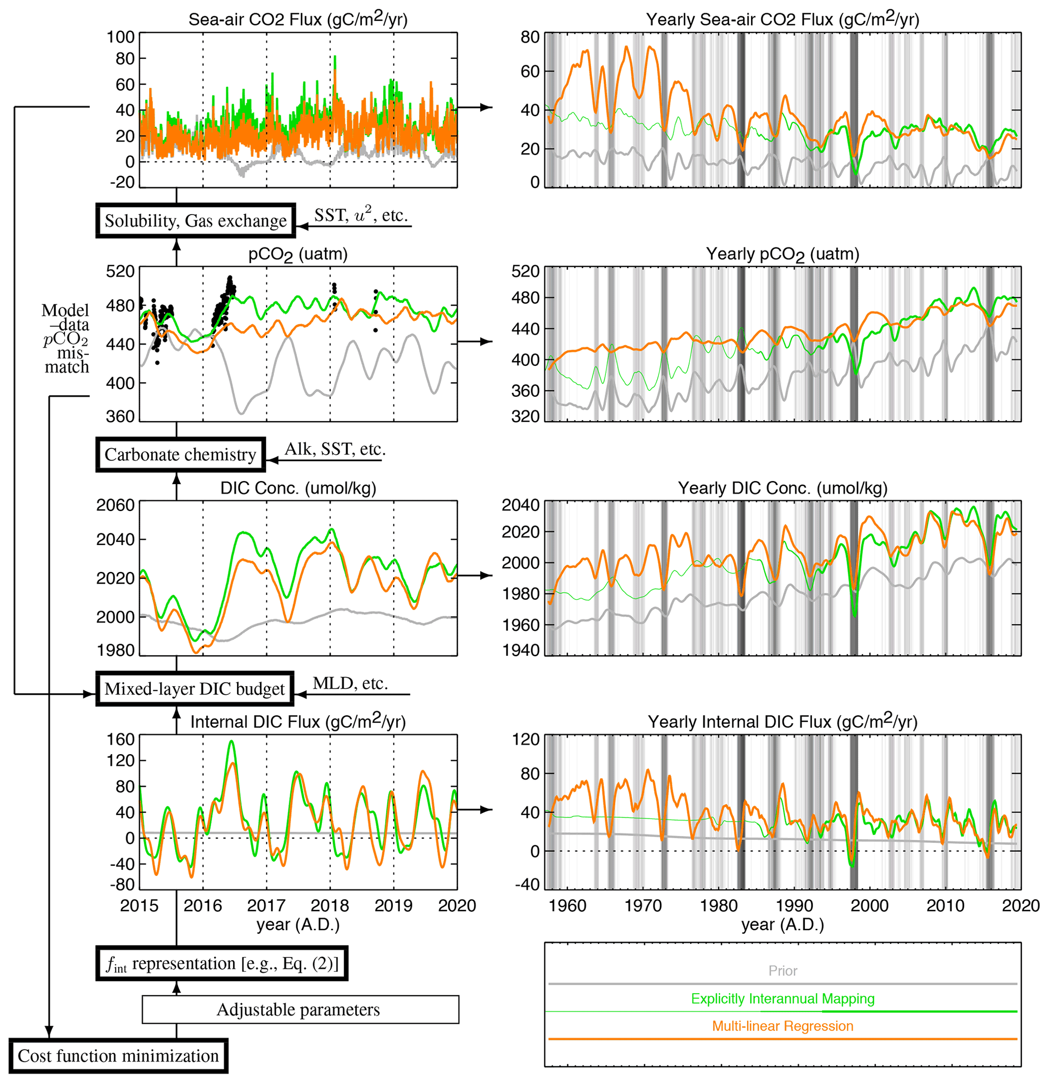
Figure 1Illustration of the quantities involved in the mixed-layer scheme (time series panels) and the calculations done to connect them (thick-framed boxes). At the arrows on the right of each calculation box, we give its most important environmental input fields (see Table 1). The time series represent the example pixel enclosing the TAO140W mooring location (2∘ N, 140∘ W) in the tropical Pacific; they are taken from the results of this study but shown here for illustration only. Left: quantities on the original daily time steps, plotted for five example years. Right: the same quantities displayed as smoothed yearly averages, which is the way all results are shown in this paper. The background shading indicates the El Niño–Southern Oscillation (ENSO) phase (multivariate El Niño index (MEI) by Wolter and Timlin, 1993).
Table 1Input data sets.
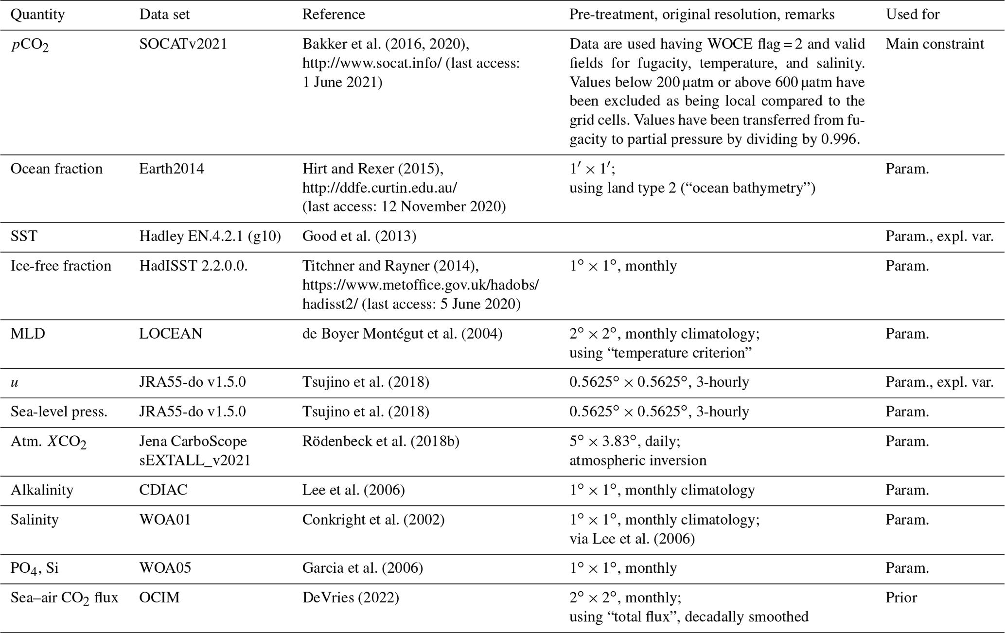
SST: sea surface temperature; MLD: mixed-layer depth; LOCEAN: Laboratoire d'océanographie et du climat: expérimentations et approches numériques; NCEP: National Centers for Environmental Prediction; SOCAT: Surface Ocean CO2 Atlas; WOCE: World Ocean Circulation Experiment; WOA: World Ocean Atlas; param.: parameterizations; expl. var.: explanatory variable.
Parameterizations of sea–air gas exchange (quadratic wind speed dependence as in Wanninkhof, 1992) and solubility (Weiss, 1974), a calculation of the chemical equilibrium of the carbonate chemistry in seawater (Orr and Epitalon, 2015) as well as a mixed-layer budget of dissolved inorganic carbon (DIC) (Rödenbeck et al., 2013), are used to express the pCO2 field and the sea–air CO2 flux field as a function of the ocean-internal flux of DIC, fint (Fig. 1). The ocean-internal DIC flux fint is meant to comprise all sources and sinks of DIC into or out of the oceanic mixed layer, through biological conversion within the mixed layer or through mixing-in of waters with different DIC concentration. It is expressed as the sum of a fixed (a priori) flux field and a set of predefined spatio-temporal patterns of adjustment each scaled by an adjustable parameter (the sets of patterns are detailed for each variant of the mapping below). Then, the mismatch between the calculated pCO2 field (at the respective pixels and time steps containing the SOCAT pCO2 samplings) and the corresponding measured pCO2 values (black dots in the pCO2 panel of Fig. 1) is gauged by a quadratic cost function. The (a posteriori) estimates of the mapping are calculated from those values of the adjustable parameters that minimize this cost function. In the example of Fig. 1, the two estimates (coloured) follow the data points (black dots) more closely than the prior (grey).
Table 2Mapping runs used in this study. The main results are given in bold; the other runs are used to assess uncertainty (“uncertainty cases”; Sect. 2.2), to illustrate specific points of discussion (“test cases”; Sect. 2.2), or to assess predictive skill (“cross-validation”; Sect. 2.3).
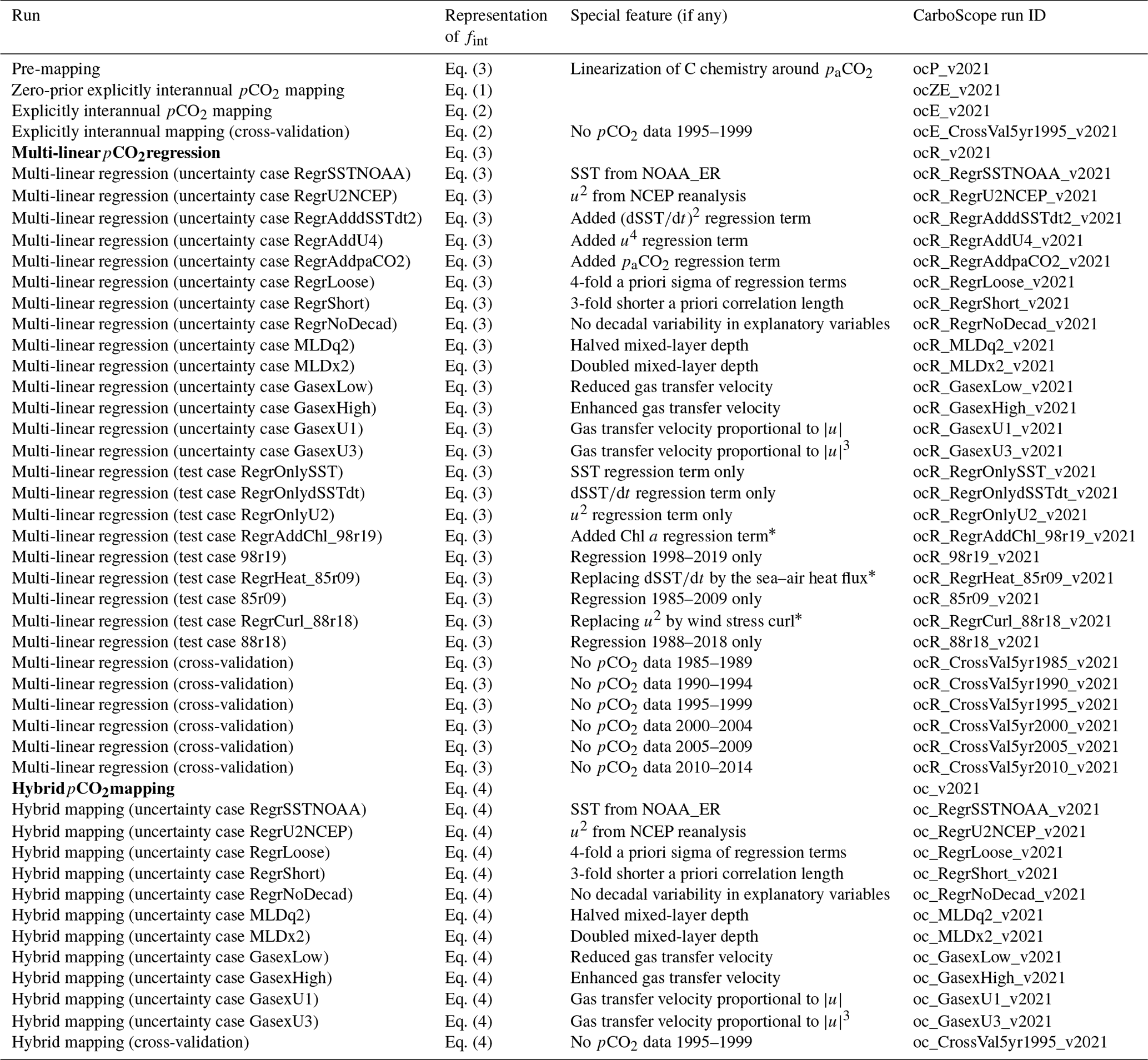
* Regression run only over 1998–2019, 1985–2009, or 1988–2018, respectively.
Spatial and temporal interpolation between the very inhomogeneously sampled data is implemented in the following way. By choosing a set of spatial patterns of adjustment that are centred at all the individual ocean pixels but simultaneously affect the respective neighbouring pixels within some correlation radius (to be detailed below), in conjunction with additional Bayesian terms in the cost function that penalize large adjustments to the adjustable parameters, the parameter fields (the ocean-internal DIC flux field or the fields of sensitivities, respectively; see below) are forced to be smooth. These smoothness constraints spread the information from data-covered pixels to neighbouring unconstrained pixels (see Fig. 5 of Rödenbeck et al., 2013), thereby interpolating spatial data gaps. (The set of patterns of adjustment indirectly defines the Bayesian a priori covariance matrix; see Rödenbeck, 2005, for background.) Interpolation in time is achieved analogously by temporal smoothness constraints (even though, for practical reasons, a mathematically equivalent Fourier formulation is used).
The four mapping variants used here (Table 2) differ in the choices of the prior for fint and the set of spatio-temporal patterns of adjustment. Our development started from a variant (Sect. 2.1.2) essentially identical to Rödenbeck et al. (2013) used as the CarboScope pCO2 mapping before version v2020, except for some technical changes described later (Sect. 2.1.6–2.1.7). As an intermediate modification, we introduced a prior stabilizing the secular trend (Sect. 2.1.3); the result of this variant will be used to help discuss specific aspects. The main results of this study come from the multi-linear regression (Sect. 2.1.4) and the hybrid mapping (Sect. 2.1.5). Figure 2 summarizes the differences and the flow of information between the four variants.
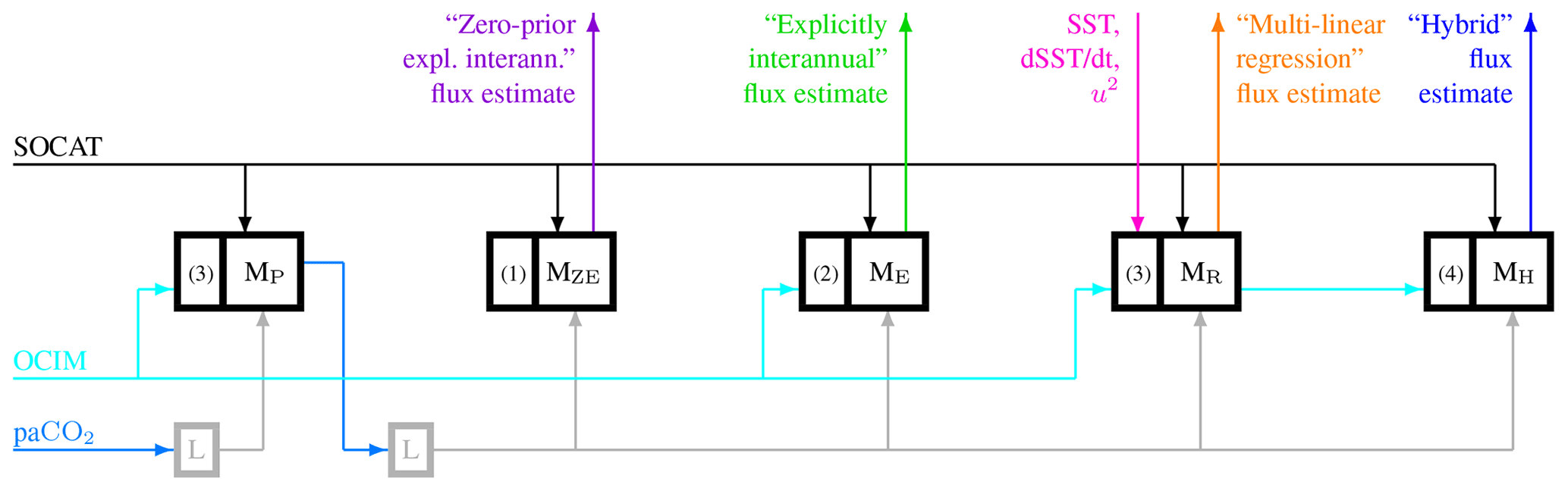
Figure 2Information flow between the presented mapping runs. Thick-framed boxes denote calculations, with arrows denoting their input and output data sets (mostly spatio-temporal fields). The violet, green, orange, and blue arrows represent the spatio-temporal sea–air CO2 fluxes estimated by our main mapping runs MZE, ME, MR, and MH (these same four colours are also used in all line plots in this paper). All mapping runs use the SOCAT database of pCO2 measurements (point data, black) as their primary information source. The runs are algorithmically identical, except for the representation of the ocean-internal DIC sources and sinks (fint) and the corresponding set of adjustable unknowns; this part of the mapping algorithm has therefore been represented explicitly as separate parts of the boxes at their left-hand sides, labelled by the respective equation number. Runs MZE and ME are using the representations with explicit interannual degrees of freedom, either without fint prior (Eq. 1) or using the decadally smoothed OCIM result as fint prior (cyan; Eq. 2). Run MR is using the representation involving regression terms (Eq. 3), which requires the explanatory variables (magenta) as further input fields; it uses the same fint prior as the run ME. The representation of fint in the “hybrid” run MH again has explicit interannual degrees of freedom but no long-term and seasonal degrees of freedom (Eq. 4). Importantly, it uses the ocean-internal DIC sources and sinks estimated by the “multi-linear regression” MR as its fint prior (cyan again). All mapping calculations use the various input fields shown in Fig. 1, which are however omitted here for clarity. More technically, the mappings also need a linearization of the non-linear dependence of pCO2 on DIC, consisting of three fields (the derivatives dpCO2 dDIC as well as reference fields for pCO2 and DIC) together depicted by the grey arrows. Box L denotes the calculation of dpCO2 dDIC and the reference DIC field from a reference pCO2 field (light blue) as described in Sect. 2.1.6 (the further input fields required by this calculation are not depicted). For the main mappings MZE, ME, MR, and MH, the reference pCO2 field comes from the data-based estimate of the pre-mapping MP. The linearization for MP, in turn, uses the atmospheric pCO2 field as pCO2 reference (light blue again).
2.1.2 The “zero-prior explicitly interannual” pCO2 mapping (ZE)
The starting variant has a general set of (many) patterns of adjustment, allowing an arbitrary smooth spatio-temporal internal DIC flux field (Rödenbeck et al., 2013). This field is implemented as the sum of a constant term (subscript “LT” for “long-term”) and terms for seasonal (subscript “Seas”) and interannual anomalies (non-seasonal, subscript “IAV”):
As indicated by the superscript “adj” or “ADJ” (difference explained below), all these terms involve degrees of freedom being adjusted in the cost function minimization sketched above. A priori, all adjustable terms are zero, such that the prior of is zero as well.
The interannual term can represent non-seasonal anomalies on all month-to-month, year-to-year, or decadal timescales, including secular trends. The level of its temporal smoothness corresponds to a priori correlation length scales of about 4 weeks, implemented through a mathematically equivalent Fourier series with dampened higher-frequency components (where Fourier terms dampened to less than 2 % are discarded entirely). This amounts to 722 scalable Fourier terms for our 71-year calculation period 1951–2021. The seasonal term only contains seasonal Fourier components; thus it only depends on the time s within the year and repeats itself every year. Along the seasonal cycle, it has the same temporal correlation length as the interannual term of about 4 weeks, amounting to 10 scalable Fourier terms. The constant term is not time-dependent by definition (1 temporal degree of freedom).
Spatially, the level of smoothness in all three terms corresponds to a priori correlation length scales of about 640 km in longitude and latitude.
As symbolized by the capitalized superscript “ADJ”, the a priori uncertainties in the seasonal Fourier terms of and are chosen to be enlarged relative to the non-seasonal Fourier terms of , corresponding to larger expected amplitudes of seasonal variations in fint compared to non-seasonal ones. In terms of the implied a priori autocorrelation function, these enhanced a priori uncertainties in seasonal variations are equivalent to non-zero temporal correlations between the flux at any given time of year and the same time of year in all other years (in addition to the 4-week decaying correlations mentioned above). Due to these periodic correlations, fint in time periods without data does not fall back to the prior (here zero) but to the mean seasonal cycle as constrained by the data-covered periods.
2.1.3 The “explicitly interannual” pCO2 mapping (E)
In order to stabilize the secular trend in the early decades (as discussed in Sect. A2 below), we now add a fixed (i.e. non-adjustable) term (superscript “fix”):
Consequently, the prior of is given by this fixed term. It is obtained from the sea–air flux product by DeVries (2022), which is based on an abiotic carbon cycle model that captures the rising atmospheric CO2 boundary condition and is embedded in a data-driven model of time-mean ocean circulation (OCIM). The OCIM fluxes have been decadally smoothed (indicated by subscript “Decad”) because the OCIM result originally represents sea–air fluxes including SST-related interannual variations, which are created by our parameterizations already (Fig. 1).
2.1.4 The “multi-linear regression” (R)
In the third variant, the ocean-internal DIC flux is represented as
Compared to Eq. (2), the degrees of freedom representing interannual variations (fint,IAV) are replaced here by a multi-linear function involving three explanatory fields (Vi):
-
sea surface temperature (SST),
-
its temporal change (), and
-
squared wind speed (u2).
There is a 2-fold motivation behind this choice of explanatory variables: (1) variations in carbon-relevant processes (e.g. carbon and nutrient input into the mixed layer, stratification, mixing, entrainment, wind-driven deepening of the mixed layer) are expected to also be related to these variables, and (2) observation-based data sets for SST and u are available over our entire calculation period 1951–2021 (u at least from reanalysis). The specific input data sets used in our base case are given in Table 1.
The simultaneous use of SST and is motivated as it is changes in SST that are related to DIC fluxes (i.e. changes in DIC). Moreover, the sum of SST and mathematically allows a temporal shift between SST and fint for a dominant Fourier mode (similar to sine and cosine terms).
To prevent confusion, we point out that the multi-linear regression as introduced here is set up in terms of the ocean-internal DIC flux fint (see Sect. 2.1.1), not in terms of pCO2 or sea–air flux as done in various other studies in the literature. This also means that important processes (SST dependence of solubility and carbonate chemistry, wind speed dependence of gas exchange) are not included into the regression Eq. (3) but are already taken care of by the parameterizations listed in Sect. 2.1.1 and Fig. 1.
All the explanatory fields Vi are implemented on a monthly timescale, smoothly transformed onto our daily time steps. The scaling factors between the internal DIC flux and these explanatory fields Vi are taken as the adjustable degrees of freedom in the cost function minimization (very analoguous to the “NEE-T inversion” of Rödenbeck et al., 2018b). These unknown scaling factors are allowed to vary spatially (with correlation length of about 2000 km in longitude and 1000 km in latitude, thus more smoothly than the direct adjustments of fint in the explicitly interannual mapping of Sect. 2.1.3), but are constant in time (1 temporal degree of freedom per explanatory field per pixel). All three regression terms are normalized such that the a priori uncertainty in their global integral on 1 July (averaged over the 1 July time steps of all years within the analysis period 1957–2020) is the same as that of fint,IAV in Eq. (2) (1 July is an arbitrary choice, in line with the normalization with respect to the flux in the middle of the final year used in CarboScope so far.)
In order to avoid influences of the spin-up transient on the regression coefficients (estimated sensitivities), the regression terms (first line of Eq. 3) only cover the analysis period 1957–2020, while the remaining years before and after are filled by explicitly interannual degrees of freedom just as in Eq. (2). For clarity, this detail has been omitted from Eq. (3).
2.1.5 The “hybrid” pCO2 mapping (H)
The final variant aims to combine the temporal extrapolation capability of the multi-linear regression (Sect. 2.1.4) and the flexibility to reproduce observed signals of the explicitly interannual mapping (Sect. 2.1.3). Technically being an explicitly interannual mapping itself, its representation of the ocean-internal DIC flux,
is similar to Eq. (2), but with the following two changes:
-
As the essential change, the interannually varying result of the multi-linear regression (Sect. 2.1.4) is used as a prior for the internal DIC flux () instead of the decadally smoothed OCIM result only containing decadal variations and the secular trend.
-
As a merely technical change, the a priori uncertainties in the mean flux and the seasonality are not enhanced with respect to non-seasonal variability any more (indicated by the lower-case superscript “adj” in all three terms) because the prior already contains a long-term mean and a mean seasonal cycle.
In essence, the hybrid mapping thus adds an interannually varying correction to the multi-linear regression. Due to this construction, the hybrid result will fall back to the multi-linear regression during periods without data, but it is nevertheless able to fit pCO2 signals on month-to-month, year-to-year, and decadal timescales that have not yet been reproduced via the explanatory variables of the multi-linear regression.
Methodological note. Mathematically, the hybrid run is equivalent to estimating the additive correction to the multi-linear regression from the pCO2 residuals of the multi-linear regression. That is, the signals being used by the hybrid run are those that could not yet be explained by the multi-linear regression. The hybrid run is thus similar to a hypothetical joint run simultaneously having regression degrees of freedom (like the multi-linear regression) and explicitly interannual degrees of freedom (like the explicitly interannual estimate). We abandoned the concept of such a joint run, however, because it would face two problems: (1) its result would depend on the relative a priori weighting between the two groups of degrees of freedom, for which there is no clear information, and (2) the explicitly interannual degrees of freedom would necessarily also absorb part of the signals actually proportional to the explanatory variables. Running the multi-linear regression and the hybrid step sequentially, as done here, reduces both problems.
2.1.6 The pre-mapping (P): determining the linearization of the carbonate chemistry
In contrast to Rödenbeck et al. (2013), we now allow for the secular trend in the Revelle factor. We deem this necessary due to our longer period of interest 1957–2020, during which the mixed-layer carbon content notably increased, leading to shifts in the relation between variations in the ocean-internal DIC flux (fint) and the sea–air CO2 flux. As our scheme extrapolates the seasonality (and in the “multi-linear regression” also the interannual variations) from the data-constrained recent decades to the almost unconstrained earlier decades through correlations in fint (see the last paragraph of Sect. 2.1.2), the shifting relation has the potential to alter the amplitude of flux variations in the earlier decades.
As in Rödenbeck et al. (2013), the non-linear dependence of pCO2 on DIC is linearized around reference fields and DICRef:
The linearization is needed to be able to use the fast minimization algorithm in the CarboScope software. Previously in Rödenbeck et al. (2013), the reference fields and DICRef were temporally constant and had been taken from observation-based data sets not guaranteed to be mutually consistent, and the derivative had been calculated from these via approximation formulas. In order to now include the secular trend in Revelle factor (and simultaneously to remove the mentioned approximations), we employ the mocsy package (Orr and Epitalon, 2015), which provides routines to accurately calculate pCO2 and from a given field of DIC (and from fields of alkalinity, SST, salinity, silicate, phosphate, and air pressure, which we take from external sources; Table 1). Using an adjusted Newton algorithm calling mocsy iteratively, we obtain an algorithm to calculate (reference) DIC and from a given (reference) pCO2 value at each location and time (box L in Fig. 2). The field is obtained as the posterior pCO2 field of a “pre-mapping” run (P, the leftmost one in Fig. 2). The and fields used in this pre-mapping run, in turn, are calculated from a preliminary reference identical to atmospheric pCO2. This yields a reasonable starting point because the atmospheric pCO2 field does already contain the secular CO2 rise, which is the most important feature in this context.
Potentially, we might expect to need a loop with further pre-mappings, each getting its field from the posterior pCO2 field of the respective previous one. However, we confirmed by explicit testing that the fields are not appreciably altered any more after the first pre-mapping; thus a single pre-mapping is sufficient.
All other mapping runs of this study use the same spatio-temporal linearization fields , DICRef, and as calculated by the pre-mapping.
2.1.7 Technical details common to all variants
As in Rödenbeck et al. (2013), the pCO2 data comprise the individual observations from file https://www.ncei.noaa.gov/data/oceans/ncei/ocads/data/0235360/SOCATv2021.tsv, last access: 1 June 2021, including all observations flagged A–D. The additional file flagged E was not used.
In contrast to Rödenbeck et al. (2013), the analysis period now starts in 1957 (chosen in light of the potential use of the results as a prior in atmospheric inversions). The actual calculation period of all runs starts in 1951. According to explicit tests, this allows the initial transient of the mixed-layer DIC budget equation to decay by 1957.
As in Rödenbeck et al. (2013), the calculation period includes 1 more year (“spin-down”, here 2021) after the valid period constrained by the data (until end of 2020), in order to avoid numerical edge effects.
In order to cover the entire calculation period since 1951, we now use SST from Hadley EN.4.2.1 (Good et al., 2013) and sea ice concentration from HadISST 2.2.0.0. (Titchner and Rayner, 2014, https://www.metoffice.gov.uk/hadobs/hadisst2/data/HadISST.2.2.0.0_sea_ice_concentration.nc.gz, last access: 5 June 2020).
Compared to Rödenbeck et al. (2013), the spatial resolution of all the mapping calculations has been increased to 2.5∘ longitude × 2∘ latitude (previously on the grid of the TM3 atmospheric transport model, 5∘ × 4∘). Moreover, the adjustments are now done over the entire ocean (i.e. we do not fix part of the temporally ice-covered regions any more).
2.2 Uncertainty and test cases
In order to explore how robust the results of the multi-linear regression (Sect. 2.1.4) are, we also perform uncertainty cases where certain set-up parameters are modified within ranges deemed as plausible as the base case (Table 2):
- RegrSSTNOAA
-
– using SST from NOAA_ERSST v5 (Huang et al., 2017) as an alternative data set for the explanatory variables SST and (but no change to any other SST-dependent items such as solubility);
- RegrU2NCEP
-
– using wind speeds from NCEP reanalysis (Kalnay et al., 1996) as an alternative data set for the explanatory variable u2 (but no change to wind-dependent gas exchange);
- RegrAdddSSTdt2
-
– additional regression term based on ()2;
- RegrAddU4
-
– additional regression term based on u4;
- RegrAddpaCO2
-
– additional regression term based on decadally smoothed paCO2;
- RegrNoDecad
-
– removing any decadal variability and secular trends from the explanatory fields Vi, such that the multi-linear regression term only represents interannual variability on a timescale of a few years;
- RegrShort
-
– shorter spatial correlation lengths for the sensitivities (Supplement Fig. S5);
- RegrLoose
-
– a priori uncertainty in the sensitivities increased by a factor of 4 (i.e. the strength of the mathematical regularization is reduced);
- MLDq2
-
– dividing mixed-layer depth by 2;
- MLDx2
-
– multiplying mixed-layer depth by 2 (lacking a clear uncertainty range of mixed-layer depth, MLDq2 and MLDx2 represent a rather strong change, maybe already outside the actual uncertainty);
- GasexLow
-
– weaker gas exchange by scaling the gas transfer velocity field such that its global mean matches the lower limit of the range 16.5±3.2 cm h−1 (Naegler, 2009) rather than the central value;
- GasexHigh
-
– stronger gas exchange (analogously, using upper limit);
- GasexU1
-
– replacing the u2 dependence of gas exchange by a dependence (while keeping the global mean gas transfer velocity the same).
- GasexU3
-
– replacing the u2 dependence of gas exchange by a dependence (while keeping the global mean gas transfer velocity the same).
To help in the discussion of specific aspects, we performed further test cases (not necessarily as plausible as the base case):
- RegrOnlySST, RegrOnlydSSTdt, RegrOnlyU2
-
– the explanatory variables used individually (i.e. the regression terms of the remaining two were omitted);
- RegrAddChl_98r19
-
– addition of Chl a as a further explanatory variable (Fig. S7; chlorophyll concentration has been taken from the GlobColour project (Maritorena et al., 2010), which combined retrievals from the SeaWiFS (NASA), MODIS (NASA), MERIS (ESA), OLCI (ESA), and VIIRS (NOAA/NASA) satellites into a harmonized data set; as the Chl a data are only available for the years 1998–2019, the regression is restricted to this period, plus spin-up and spin-down periods);
- RegrHeat_85r09
-
– replacing with the net sea–air heat flux taken from the OAFlux project (Yu and Weller, 2007); regression period restricted to 1985–2009 according to the availability of the heat flux data set;
- RegrCurl_88r18
-
– replacing u2 with wind stress curl calculated from Cross-Calibrated Multi-Platform (CCMP) v2.0 wind speeds (Atlas et al., 2011); regression period restricted to 1988–2018 according to the availability of CCMP;
- 98r19, 85r09, 88r18
-
– using the same regression terms as in the base case but restricting the time period of regression to the same years as used for RegrAddChl_98r19, RegrHeat_85r09, and RegrCurl_88r18, respectively.
Uncertainties in the hybrid mapping (Sect. 2.1.5) were explored analogously by re-running the hybrid step with several of the uncertainty cases of the regression listed above (Table 2). Part of the involved set-up changes (mixed-layer depth, gas exchange) also affect the hybrid calculation itself.
2.3 Gauging the predictive skill of the multi-linear regression
In order to test whether the multi-linear regression against explanatory variables (Sect. 2.1.4) is actually meaningful, we determine its predictive skill. For this, the multi-linear regression is re-run six times, each time omitting the pCO2 data from one of the 5-year periods 1985–1989, 1990–1994, 1995–1999, 2000–2004, 2005–2009, or 2010–2014. That is, each of the six test runs possesses an artificial data gap of 5 years, a duration chosen to be longer than typical features of year-to-year variability like El Niño. We can then compare the predictions during the data gaps with the results of the completely constrained run.
The main results of this study are of two different types:
-
From the multi-linear regression, we obtain spatial maps of the sensitivities γi (Eq. 3) relating the variations in the surface-ocean carbon system to variations in SST, , and u2 (Sect. 3.2).
-
The hybrid mapping yields a spatio-temporal estimate of the sea–air CO2 flux over 1957–2020, in particular its evolution from year to year (Sect. 3.5).
Further results are presented for illustration and to elucidate the robustness of the main results.
3.1 Origin of interannual variations as estimated by the multi-linear regression
The multi-linear regression attempts to trace the interannual variations in the surface-ocean carbon system (and hence in the sea–air CO2 flux) to the interannual variations in the chosen explanatory variables SST, , and u2. In Fig. 3 (left panels), the estimated contributions of the three explanatory variables to the ocean-internal DIC flux are depicted for a subdivision of the ocean into five latitudinal bands. In the centre panels, the resulting contributions to the sea–air CO2 flux are shown, as calculated by the parameterizations and the budget equation in our mapping scheme (Sect. 2.1.1). These contributions and the prior sum up to the total sea–air CO2 flux, shown in the right panels together with our set of uncertainty results (Sect. 2.2).
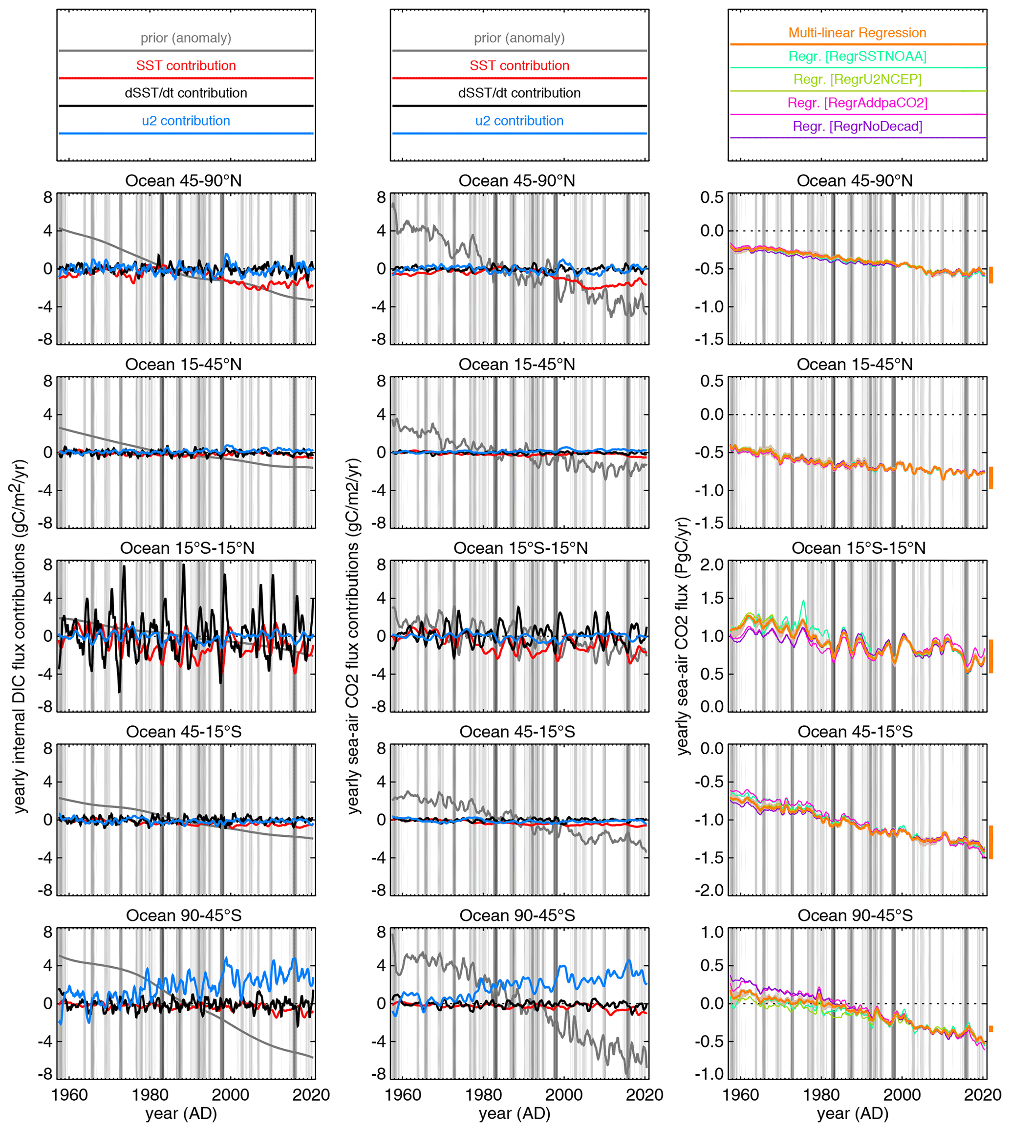
Figure 3Left: estimated contributions of the three explanatory variables in the multi-linear regression (as well as the prior, plotted here without its mean) to the ocean-internal DIC flux in five latitudinal bands (top to bottom). Centre: corresponding contributions to the sea–air CO2 flux. Right: total sea–air CO2 flux estimated by the multi-linear regression (base case, orange) together with the uncertainty cases listed in Sect. 2.2 (the cases with the largest impact on interannual variability – RegrSSTNOAA, RegrU2NCEP, RegrAddpaCO2, RegrNoDecad – are plotted explicitly in different colours; since the cases related to gas exchange – GasexLow, GasexHigh, GasexU1, GasexU3 – shift the long-term mean of the flux, the range of this shift has been indicated by the length of the vertical orange bars just to the right of each panel for clarity; the remaining uncertainty cases having rather small impact – RegrAdddSSTdt2, RegrAddU4, RegrLoose, RegrShort, MLDq2, MLDx2 – have been subsumed into the pale orange band depicting their envelope). All curves show interannual variations. The background shading indicates the El Niño phase according to the multivariate El Niño index (MEI) by Wolter and Timlin (1993). In the left and centre panels, fluxes are given in per-area units to emphasize the local process perspective, while fluxes in the right panels are given as regional integrals to emphasize their share in the total ocean flux.
When disregarding the secular increase in the ocean carbon sink, the largest year-to-year variations in the regionally integrated sea–air carbon flux are found in the tropics (Fig. 3, middle right), in particular the tropical Pacific (Fig. S4). Correspondingly, the year-to-year variations in the ocean-internal carbon flux (fint) from the three terms in the multi-linear regression (Eq. 3) are largest in the tropics as well (Fig. 3, middle left). Of the three explanatory variables, the contribution of year-to-year variability in temporal SST changes (, black) is the largest. Concurrent with the warming (dSST dt>0) at the onset of each El Niño event (grey background stripes), we find a negative carbon flux anomaly (reduction in the carbon source in this region) because smaller amounts of cold, carbon-rich water are upwelling. At the end of each El Niño event, we find an analogous coupling of the cooling (dSST dt<0) and an additional carbon source to the mixed layer. The contribution of year-to-year variability in SST itself (red) is second-largest in the tropics, causing anomalous carbon sinks during El Niño events and anomalous carbon sources during La Niña conditions afterwards. This could be interpreted as a small correction to the contribution: the sum of the and SST contributions (not shown) is similar to the contribution alone but slightly shifted in time by a few months. The smallest contribution to the year-to-year variability in the tropics is estimated for squared wind speed (u2, light blue), with a temporal pattern relatively similar to that of the SST contribution. Due to the co-variation between SST and u2 on a year-to-year timescale, these two explanatory variables could be partly confounded by the regression, though the detailed locations where their respective sensitivities are high do not actually overlap much (see Sect. 3.2 below).
In the high-latitude bands (top and bottom left panels of Fig. 3), the wind speed contribution is estimated to be larger than in the tropics, now on the same order of magnitude as the SST and contributions or even larger. As a notable feature in the Southern Ocean (bottom left), the secular increase in wind speed leads to a secular increase in the carbon source into the mixed layer. Across our set of uncertainty cases (Sect. 2.2), the linear trend of the wind speed contribution over the 1960–2019 period in the ocean south of 45∘ S is estimated in the range 0.002 to (see Supplement Fig. S3, bottom, light-blue bars). As a secular trend in fint (bottom left in Fig. 3) causes a secular trend in sea–air flux of the same size (bottom centre), it represents a reduction by 17 % to 42 % of the trend towards an increasing Southern Ocean sink strength (relative to the trend of estimated by OCIM over 1960–2019). A slowing-down of the Southern Ocean sink increase (compared to the increase expected from rising atmospheric CO2) has also been found in model simulations and attributed to an increase in upwelling of old carbon by the accelerating winds (Le Quéré et al., 2007; Hauck et al., 2013; and many others). We need to note, however, that our multi-linear regression estimates the wind-speed-related trend only indirectly: as the sensitivities are presumably largely constrained by year-to-year variations (because they do not change much if the linear trend of the explanatory variables is removed; see sensitivity case RegrNoDecad, Sect. 4.3), the slope of the secular trend can only be correct to the extent that the sensitivity is identical for year-to-year and secular variations.
The year-to-year anomalies from the fint contributions (Fig. 3, left) carry through to the sea–air CO2 flux (centre) in a delayed and dampened fashion due to the buffer effect of carbonate chemistry in combination with the limited gas exchange. We also note again that the sea–air CO2 flux contains additional year-to-year variability from solubility and gas exchange anomalies as represented by the involved parameterizations (also see Fig. 1 and Sect. 3.2.4 below).
3.2 Patterns of the sensitivity of ocean-internal DIC sources and sinks to interannual variations in SST, , and u2 estimated by the multi-linear regression – which underlying processes do they suggest?
The estimated sensitivities of the ocean-internal DIC flux (fint) against interannual variations in the chosen explanatory variables of the multi-linear regression (sea surface temperature SST, temporal changes in sea surface temperature , and squared wind speed u2) are shown in Fig. 4. Here we consider the most prominent features in these sensitivity patterns and mention oceanic processes that are compatible with these and may thus control surface-ocean biogeochemistry. Even though regression analysis cannot prove causation, we argue later (Sect. 4.1) why such a tentative attribution may be meaningful here. Also see Sect. 4.3–4.6 for further discussion on uncertainties.

Figure 4Estimated sensitivities of the ocean-internal DIC flux fint against interannual variations in the temporal changes in sea surface temperature (a), in the sea surface temperature itself (b), and in squared wind speed (c). Positive (negative) sensitivities mean that increases in the respective explanatory variable are associated with a stronger source (stronger sink) of DIC in the mixed layer.
3.2.1 Sensitivity of fint to
We start with (Fig. 4, top) as the explanatory variable contributing the largest year-to-year variability (Sect. 3.1). Events of decreasing SST are estimated to be associated with more positive ocean-internal DIC fluxes in the tropical Pacific (within a tilted band located around the Equator in the western tropical Pacific and around about 15∘ S in the eastern tropical Pacific) and in most parts of the higher latitudes in both hemispheres (blue and cyan areas in Fig. 4a). Such a correlation would arise from variations in the upwelling of waters that are both colder and more carbon-rich than the mixed layer.
In the rest of the ocean, the absolute value of the sensitivity is small (light blue or light red). We assume that these sensitivities mainly reflect insignificant correlations, especially due to the higher uncertainty in regions of sparse data coverage or in regions where is mainly driven by atmospheric heating or cooling. In particular, positive sensitivities are not compatible with any known oceanic mechanism.
3.2.2 Sensitivity of fint to SST
The estimated sensitivity γSST between the interannual variations in the ocean-internal DIC flux and SST itself is rather patchy, with both positive and negative areas (Fig. 4, middle). This may reflect the fact that various biological processes contribute to fint, depending on temperature in different ways and thus potentially cancelling each other. For example, carbon fixation (net primary productivity, NPP) will invigorate with increasing temperature (until a threshold is reached); as NPP represents a sink (i.e. a negative contribution to fint), it would thus cause negative γSST sensitivities. Carbon export (or export ratio at least) is generally anticorrelated with temperature (Laws et al., 2000), thus causing positive γSST sensitivities, though also the opposite behaviour seems possible.
Positive interannual sensitivity to SST would also be compatible with a nutrient effect. Upwelling and mixing-in from below both decreases SST and increases the availability of nutrients. Thus, negative anomalies in SST tend to be associated with higher biological production and thus enhanced removal of carbon (negative anomalies in fint). However, upwelling also brings up carbon, which is usually assumed to dominate the carbon signal. For example, Hauck et al. (2013) showed that – in the model – in the Southern Ocean south of 55∘ S, there would be more biological export per increase in the Southern Annular Mode (SAM), which goes along with more upwelling. Yet, whether the carbon effect or the opposing nutrient effect dominates the upwelling signal is still controversially discussed.
As the statistical inference by our regression can only respond to the sum of all contributing processes, we therefore cannot draw specific conclusions from the estimated γSST pattern. In addition, the regression may adjust γSST to effectively shift the contribution in time (Sect. 3.1).
3.2.3 Sensitivity of fint to u2
Higher wind speeds are estimated to be associated with more positive ocean-internal DIC fluxes (stronger sources into or weaker sinks out of the mixed layer) along the Equator in the Pacific; in the eastern upwelling zones of the North Pacific, South Pacific, and South Atlantic; and in circumpolar bands in the high latitudes of both hemispheres (red and yellow areas in Fig. 4c). Such a positive sensitivity is compatible with wind-driven deepening of the mixed layer, Ekman pumping, or speeding-up of the wind-driven upwelling, such that more carbon-rich waters are mixed in from below during stronger winds.
In contrast, higher wind speeds tend to be associated with more negative ocean-internal DIC fluxes (i.e. weaker sources or stronger sinks) at the western extratropical fringes of all ocean basins (blue areas). In these regions of mode water formation, higher wind speeds lead to more subduction of anthropogenic CO2 away from the surface into the ocean interior.
3.2.4 Additional variability in the sea–air flux
We note again that the sensitivities discussed here are those of the ocean-internal DIC sources and sinks fint (Fig. 1 bottom or Fig. 3 left). The sea–air CO2 fluxes (Fig. 1 top or Fig. 3 centre) contain additional variability also driven by interannual variations in SST (e.g. via the changes in CO2 solubility and chemical equilibrium) or in wind speed (via the gas transfer velocity of gas exchange). As this additional variability is already generated by the parameterizations contained in our algorithm (Sect. 2.1.1), these processes are, within uncertainties, not reflected in the sensitivities against SST or u2 again.
Even though the sea–air CO2 flux is the quantity most directly relevant to the atmospheric CO2 budget and its consequences for global climate, this additional variability partly disguises the variability caused by ocean-internal processes as those discussed above. This also means that the ocean-internal DIC sources and sinks fint are potentially easier to be related to environmental variables than the sea–air CO2 flux or the pCO2 field traditionally chosen as a target variable of linear or non-linear regressions because it is a directly observed quantity.
3.3 How much predictive skill does the multi-linear regression have?
The results of the multi-linear regression are only meaningful if the regression actually possesses some predictive skill to bridge unconstrained periods. Only then can they be considered to represent generalizing relationships.
In order to test this, we performed runs with artificial data gaps of 5 years length (Sect. 2.3). Figure 5 illustrates this using runs discarding all pCO2 data during 1995–1999. For context, we first consider the explicitly interannual mapping (E), which draws all information about year-to-year variations from the data and therefore does not have any predictive skill. Indeed, it essentially defaults to the prior (having upside-down El Niño response as it misses any variations related to the ocean-internal sources and sinks) during the data gap (Fig. 5a), except for a shift in long-term mean (see Sect. 2.1.2, last paragraph, for explanation). In contrast, the multi-linear regression (Fig. 5b) almost completely reconstructs the 1995–1999 flux variations based on the relationships between the ocean-internal DIC flux and the driving variables learned on the basis of the remaining data outside 1995–1999.
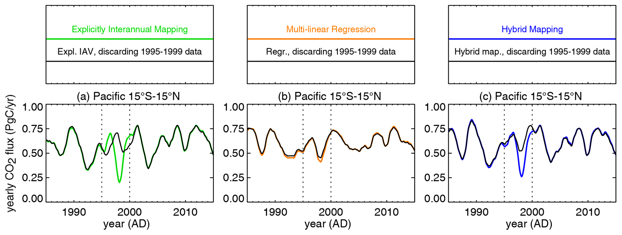
Figure 5Interannual variations in the sea–air CO2 flux in the tropical Pacific estimated by the explicitly interannual mapping (a), the multi-linear regression (b), and the hybrid mapping (c), using either all pCO2 data (base cases, colour) or all data but the ones during 1995–1999 (black).
As demonstrated by Fig. S1 in the Supplement, this predictive skill generally holds for all parts of the ocean and other 5-year data gaps. This means that no particular pCO2 data point is causing features in the variability and the estimated sensitivities (Sect. 3.2 above) by its own.
3.4 Sea–air CO2 flux variations estimated by the hybrid mapping
After presenting the interannual sensitivities from the multi-linear regression, we now turn to interannual flux variations as estimated by the hybrid mapping involving an additional interannually varying correction (Sect. 2.1.5). Figure 6 (blue) shows its estimated interannual (i.e. slower-than-seasonal) variations in the sea–air CO2 flux, subdividing the ocean into basins and latitude bands.
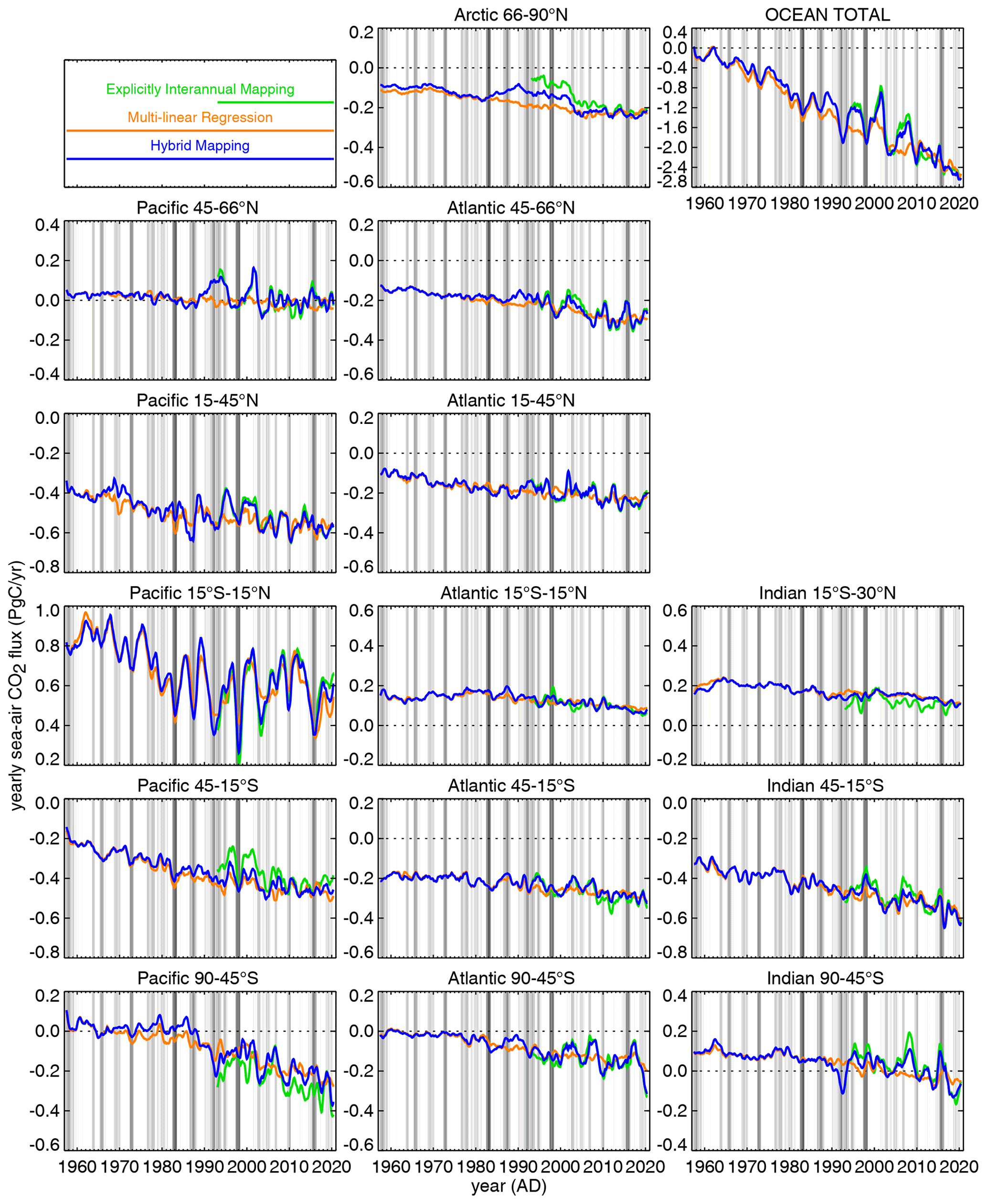
Figure 6Yearly sea–air CO2 flux as estimated from pCO2 data by the explicitly interannual mapping (green; discarded before 1985, when the data constraint is very weak), the multi-linear regression (orange), and the hybrid mapping (blue). Fluxes have been integrated over a set of regions subdividing the ocean into basins (left to right) and latitude bands (top to bottom). For better temporal orientation across panels, the grey vertical background stripes indicate the positive phases of El Niño–Southern Oscillation according to the multivariate El Niño index (MEI) by Wolter and Timlin (1993).
The most prominent feature of interannual variability is the secular trend towards more CO2 uptake in all ocean regions. Considering variations around this secular trend, the tropical Pacific is the region providing the largest contribution to total ocean variability (compare Le Quéré et al., 2000) on both a decadal timescale and a year-to-year timescale. The year-to-year variations are strongly tied to El Niño as indicated by the background stripes (Feely et al., 1999). When considering trends within individual decades, the decadal increase in the CO2 sink slowed down in the 1990s and early 2000s and accelerated again afterwards (Landschützer et al., 2016; DeVries et al., 2019), even though it may be questioned whether such trends over chosen 10-year periods truly represent decadal variations rather than apparent trends arising from high-amplitude anomalies on the faster year-to-year timescale.
3.5 How do the year-to-year sea–air CO2 flux variations estimated by regression and hybrid mapping compare with each other?
In addition to the variations in the sea–air CO2 flux estimated by the hybrid mapping (blue), Fig. 6 also shows those estimated by the multi-linear regression (Sect. 2.1.4, orange) and the explicitly interannual pCO2 mapping (Sect. 2.1.3, green). From the late 1980s onwards, when progressively more pCO2 data are available to constrain interannual variations explicitly, the hybrid mapping (blue) shows some corrections over the multi-linear regression (orange). For the large El Niño-related variability in the tropical Pacific, these corrections are generally small compared to the estimated variations themselves. This indicates that the multi-linear regression already captures a notable fraction of the year-to-year flux variations in this region, even though it underestimates the size of most of these anomalies (the interannual standard deviation between 1985 and 2019 from the multi-linear regression is only about 82 % of that from the hybrid mapping in the tropical Pacific). Figure 7 (dots) confirms that the hybrid mapping fits the pCO2 data closely (the blue dots are located right under the black dots), while the multi-linear regression (orange dots) also follows the variability in the data (black dots) but does not match them as closely as the hybrid mapping.
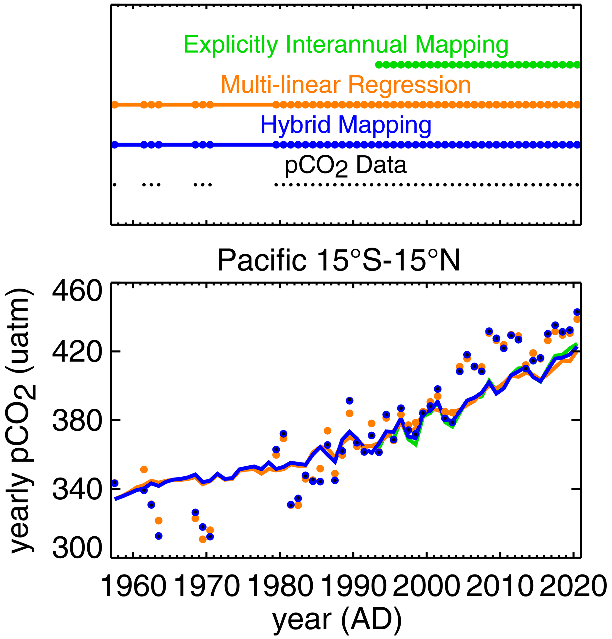
Figure 7Estimated pCO2 in the tropical Pacific, averaged spatially and over calendar years. The coloured lines give full regional averages from the explicitly interannual mapping (green), the multi-linear regression (orange), and the hybrid mapping (blue). The coloured dots are from the same estimates but averaged only over the pixels and time steps covered by pCO2 data in the respective year. The smaller black dots give the corresponding averages over the data. We note that the green, blue, and black dots are not visible individually because they are almost exactly located on top of each other, indicating that the model–data residuals of the explicitly interannual and hybrid mappings are very small. The differences between dots and lines reflect the bias of the incompletely sampled average compared to the full regional average, which the mapping algorithm is trying to address.
In the intermediate and high latitudes (top and bottom panels of Fig. 6), in contrast, the multi-linear regression (orange) does not pick up most of the year-to-year anomalies. This may indicate that the set of explanatory variables used in the regression misses essential modes of variability there. However, some of the variations estimated with explicitly interannual degrees of freedom (green and blue) may also be spurious effects from the temporally very uneven data coverage.
Although the hybrid mapping (blue) has the same interannual degrees of freedom (i.e. the same flexibility) as the explicitly interannual mapping, it does not always bring the fluxes back to the explicitly interannual result (green), especially in the region south of the tropical Pacific (Fig. 6). Since the two estimates are actually very close to each other where data exist (as illustrated in Fig. 7; the green dots are essentially invisible under the co-located blue and black dots, despite the differences between the green and blue lines), the differences in areal averages as in Fig. 6 reflect differences in data-void areas and periods being filled by the mappings. However, while the explicitly interannual mapping falls back to the prior not constrained by pCO2 data, the hybrid mapping falls back to the multi-linear regression, which is at least indirectly constrained via the statistical relationships between the ocean-internal DIC flux and the chosen explanatory variables (Sect. 3.3 above). This may also prevent some undue spatial extrapolation from the tropical Pacific into unconstrained areas by the explicitly interannual scheme. Thus, we expect the hybrid mapping (blue) to be more realistic than the multi-linear regression and the explicitly interannual mapping in terms of their detailed interannual anomalies.
In view of applying the multi-linear regression as a prior of the hybrid mapping, its predictive skill (Sect. 3.3) is only meaningful to the extent that it is actually able to explain all signals in the data. For example, since the regression underestimates the year-to-year anomalies in the tropical Pacific compared to the explicitly interannual estimate as discussed above, it will fill data gaps with somewhat too small an amplitude (Fig. 5c). This indicates that the variability extrapolated into the earlier decades without data will likely be underestimated, too, even though this is still a clear qualitative improvement compared to the explicitly interannual mapping (Fig. 5a).
3.6 What can the pCO2 mappings say about the secular flux trend?
In light of climate change, quantitative information about the secular flux trend is relevant. Unfortunately, as discussed in more detail in the appendix (Sect. A2), the secular trend in our mapping results is mostly determined through the prior derived from the OCIM estimate based on ocean interior data (DeVries, 2022). Due to the lack of pCO2 data in the early decades, the mapping does not add credible information about the secular trend. Due to some slight inconsistency in the use of the prior, the secular trend is even slightly overestimated (Sect. A2); this remains to be addressed in future versions of our flux product.
4.1 How meaningful is the multi-linear regression in terms of biogeochemical processes?
Statistical inferences by multi-linear regression are at the risk of overfitting, i.e. adjustment of coefficients to follow minor signals in the data, or even noise. If that was the case, the estimated sensitivities would not reflect underlying biogeochemical processes. Various findings indicate however that the results of the presented multi-linear regression do reflect actual signals:
-
The patterns of the sensitivities (Fig. 4), at least those with respect to and u2, are quite systematic spatially and in many respects interpretable (Sect. 3.2). This is especially true in the tropical Pacific, but also throughout the entire ocean.
-
Test regression runs only using one of the explanatory variables (RegrOnlySST, RegrOnlydSSTdt, RegrOnlyU2) yield sensitivities very similar to the base case using all explanatory variables (Supplement Fig. S2). This indicates that the regression terms are essentially mutually independent, such that each explanatory variable picks up a more or less unique portion of the signals contained in the data.
-
The regression possesses predictive skill (Sect. 3.3 above), which also means that it does not depend on any particular portion of the pCO2 data or the explanatory fields alone.
-
The estimates are relatively robust against alternative data sets for the explanatory variables (cases RegrSSTNOAA and RegrU2NCEP in Supplement Fig. S4). This corroborates the notion that the regression is likely not dominated by any particular feature in these fields.
-
The regression hardly responds to a 4-fold change in the regularization strength (case RegrLoose in Supplement Fig. S4). In the overfitting regime, one would expect a substantial dampening effect when the regularization is stronger.
-
The regression results are quite robust against further changes in the set-up (Supplement Figs. S4, S5, and S6).
The relatively small set of explanatory variables used here (Sect. 2.1.4) is certainly helpful to avoid overfitting as it means a relatively small number of degrees of freedom (cf. Thacker, 2012). Also the use of temporally constant sensitivity coefficients helps to keep the number of degrees of freedom sufficiently low. For example, in test runs with seasonally resolved sensitivity coefficients, the data could be fitted more closely but the predictive skill deteriorated (not shown).
Clearly, for any given spatial area, the presence of pCO2 data over a sufficient variety of environmental conditions is a prerequisite to estimate meaningful sensitivity coefficients. The “reduction in uncertainty” diagnostic for interannual variations given in Rödenbeck et al. (2014) provides at least a rough indication. A reduction-in-uncertainty diagnostic could also be performed for the sensitivity coefficients directly, which however remains for follow-on work.
4.2 Which fraction of the year-to-year variability can be captured by the multi-linear regression?
As seen in Fig. 6 and quantified explicitly in Fig. 8 (top), the amplitude of year-to-year variability in the global sea–air CO2 flux estimated by our multi-linear regression (orange) is lower than that estimated by the hybrid mapping possessing the degrees of freedom to follow any interannual signals (blue). This indicates that the pCO2 data also contain signals of year-to-year variability that cannot be represented in terms of the variations contained in the set of explanatory variables used in the regression. Possibly, however, the hybrid mapping may also exaggerate the amplitude of signals by spreading them over too large an area in data-poor parts of the ocean.
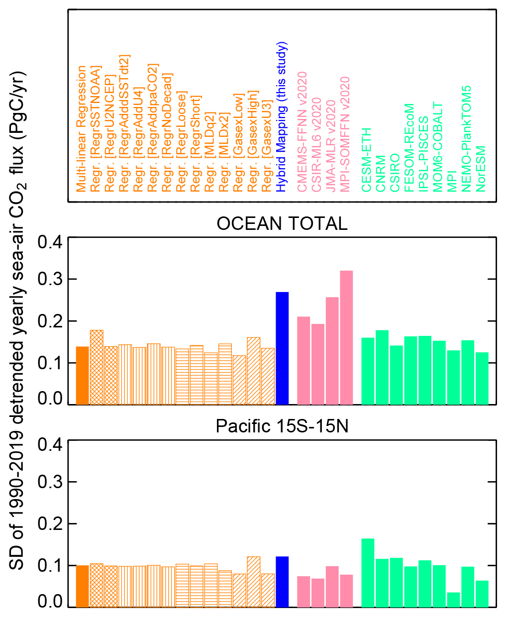
Figure 8Amplitudes of variability in the sea–air CO2 flux on year-to-year timescales around its secular trend, from the multi-linear regression (orange group of bars; solid: base case; hashed: uncertainty cases) and the hybrid mapping (blue), compared to other pCO2 mapping methods (salmon; CMEMS v2020, Denvil-Sommer et al., 2019; CSIR-ML6 v2020, Gregor et al., 2019; JMA-MLR v2020, Iida et al., 2020; and MPI-SOMFFN v2020, Landschützer et al., 2013) as well as the ocean biogeochemical process models collated in Friedlingstein et al. (2020) (mint green). The amplitudes are represented by temporal standard deviations of detrended yearly fluxes over the 1990–2019 period. The top panel gives the global flux, the bottom panel the tropical Pacific.
The situation is different in the tropical Pacific (Fig. 8, bottom). Here, the multi-linear regression (orange) already captures a large part of the variability found in the hybrid mapping (blue). This indicates that our explanatory variables are reasonably suited to represent the ENSO-related variability dominating in this region.
To elucidate the ability of the multi-linear regression to capture year-to-year anomalies, we compare it with other pCO2 mappings based on linear or non-linear regressions of pCO2 (itself) against various sets of explanatory variables (Landschützer et al., 2013; Iida et al., 2020; Denvil-Sommer et al., 2019; Gregor et al., 2019). Globally (Fig. 8, top), the variability obtained by the other pCO2 mappings (salmon) is larger than that from our multi-linear regression (orange). Closer inspection (not shown) reveals that these larger amplitudes mostly reflect variability on multi-year (decade-to-decade) timescales occurring coherently in both northern and southern extratropics, while the multi-linear regression does not involve such globally correlated contributions. Accordingly, when splitting up the global flux into regional contributions, the amplitudes from the other pCO2 mappings and our multi-linear regression are quite comparable. For example, in the tropical Pacific (Fig. 8, bottom) our regression yields year-to-year variability larger than any of the other pCO2 mappings considered. Based on reconstructions of model-based pseudo-data, Gloege et al. (2021) found for one of the other methods included in Fig. 8 that the amplitude of Southern Ocean decadal variability was overestimated by 15 % to 58 %.
Could alternative or additional explanatory variables help to capture a larger fraction of variability by the multi-linear regression?
-
As the explanatory variables of the base case are all physical variables, we tested using chlorophyll a concentration as a biological variable (run RegrAddChl_98r19; Supplement Fig. S7). A practical problem with chlorophyll a is that data sets are only available for the most recent years (from 1998); therefore it is not used in our base case. The test suggests, however, that chlorophyll is not actually adding much information about the year-to-year variations in the sea–air CO2 flux beyond what is already provided by the explanatory variables of the base case (SST, , and u2). A reason may be that chlorophyll variability is already covered in the other variables as nutrients are also a function of upwelling, stratification, etc. It is also important to keep in mind that chlorophyll concentration is not directly observed but only indirectly inferred from optical properties of the seawater. Due to that, part of the variability in the chlorophyll data may originate from processes unrelated to the carbonate system, which makes it less helpful as a predictor in the regression considered here.
-
Conceivably, more general non-linear relationships between pCO2 and the explanatory variables may allow the capturing of signals not represented in linear relationships as used in our base case. Uncertainty cases involving additional regression terms proportional to ()2 (run RegrAdddSSTdt2) and (u2)2 (run RegrAddU4), respectively, only marginally increase year-to-year variability (within the narrow band in Fig. S4). Also from the set of other pCO2 mappings (salmon in Fig. 8), there is no indication that the non-linear regressions (CMEMS-FFNN, CSIR-ML6, and MPI-SOMFFN) would generally capture more variability than the linear ones (JMA-MLR and ours). We conclude that non-linearities in the pCO2 relationships are not essential for explaining year-to-year anomalies in the pCO2 field on a regional scale.
-
Using heat flux as an explanatory variable instead of (RegrHeat_85r09) deteriorates the ability of the multi-linear regression to reproduce ENSO-related variability (Supplement Fig. S8).
-
Replacing u2 by the wind stress curl (RegrCurl_88r18) does not change the flux IAV much (Supplement Fig. S10). A further alternative explanatory variable may be “Ekman pumping”, which however diverges at the Equator and was not tested.
A common methodological feature of all present-day regression-based pCO2 mappings including ours is that the carbon variables are only related to the concurrent values of the explanatory variables, disregarding any dependence on past values of the explanatory variables possible due to memory effects. This might be a serious limitation, but allowing for memory effects is not straightforward. For example, regression terms with lagged explanatory variables would only allow discrete lag times, and using an extensive spectrum of lag times would possibly exceed the number of well-determined degrees of freedom. Theoretically, fitting comprehensive process models to the pCO2 data would include emerging memory effects, but this faces various conceptual and computational challenges (see a recent application of a low-dimensional Green's function approach by Carroll et al., 2020). (Note that the amplitudes simulated by the hindcast ocean biogeochemical models included in Fig. 8 are roughly similar to those from our multi-linear regression and smaller than those from the hybrid scheme.) We notice that our algorithm involves some elements that do represent history effects (the budget equation Eq. A18 in Rödenbeck et al., 2013, accumulating past fint contributions; the seasonal “history flux” Eq. A20 in Rödenbeck et al., 2013; and the use of both SST and as explanatory variables; see Sect. 3.1 above). However, if memory effects are important, they are evidently not yet adequately captured by those elements.
4.3 To which extent do the sensitivities γi depend on the timescale?
In our formulation of the regression (Eq. 3), the sensitivities γi are applied to the fields Vi of the explanatory variables including all their variations on year-to-year, decadal, and secular timescales. Conceivably, however, the relationships between fint and the explanatory variables may differ for year-to-year, decadal, or secular variations. In ocean areas where the data period is long enough to possibly constrain decadal timescales directly, the estimates may therefore reflect some mixture of timescales, which would be hard to interpret.
We assessed this by the uncertainty case RegrNoDecad, where any decadal variability (including any secular trend) has been removed from the three explanatory variables. As this case can only pick up year-to-year signals to constrain the sensitivities, any changes compared to the base case may indicate such potential timescale conflicts. In most regions, this is not evident (Supplement Fig. S6). Exceptions are the southern Pacific and the tropical Indian (for the wind-speed sensitivity ) and the western tropical Pacific (for the SST sensitivity γSST). As the explanatory variable , which dominates the large tropical variability, does not have much secular trend, it is not prone to timescale dependence anyway.
An alternative way to assess the impact of secular trends in the explanatory variables is the uncertainty case RegrAddpaCO2 having an additional regression term proportional to decadally smoothed atmospheric CO2 (paCO2). As paCO2 is rising steadily over the calculation period, this run is able to adjust the secular trend independently of the trends in SST, , or u2, thus breaking any potential timescale conflicts. Indeed, the sensitivities estimated by RegrAddpaCO2 (not shown) are similar to those from the base case as well, and any differences from the base case are similar to those of RegrNoDecad.
We note that in ocean areas with data periods of a few years only, a possible timescale dependence will not affect the sensitivities themselves, but it may still affect secular trends in the fluxes if sensitivities estimated for year-to-year variations are applied to secular trends in the explanatory variable. We do not have a means to detect whether this is the case.
4.4 Spurious effects from uncertainties in the parameterizations
Errors in the sea–air CO2 flux resulting from deficiencies in our chosen parameterizations of solubility and gas exchange lead to compensating spurious contributions to fint because it is the sum of both fluxes which changes the mixed-layer carbon content in our budget equation (see Fig. 1 or Rödenbeck et al., 2013). This will then also lead to spurious contributions to the estimated sensitivities γi. For example, spurious u2 sensitivity may arise if the wind speed dependence of our gas exchange parameterization is not strong enough such that it is reinforced by additional changes in the ocean-internal carbon flux (or vice versa).
Luckily, the interannual variability in the sea–air CO2 flux is much smaller than that of fint due to the buffer effect (see Fig. 1). Therefore, in relative terms, the error in the sea–air CO2 flux translates into a much smaller error in fint and in the sensitivities γi.
4.5 Spurious effects from missing interannual alkalinity variations
The estimated ocean-internal DIC flux fint – and thus the estimated sensitivities γi in the regression – contains some spurious contributions to compensate any errors in our representation of carbonate chemistry because the pCO2 data constrain the pCO2 field rather than the DIC field (Fig. 1). Even though we represent the carbonate chemistry – up to the linearization – by exact equations (Sect. 2.1.6), some error arises because we only use a seasonal alkalinity climatology, while alkalinity also varies interannually due to (1) changing degrees of dilution due to freshwater fluxes (evaporation, precipitation, ice formation, and ice melt) as well as (2) mixing-in of alkalinity-rich deep waters and possibly biological influences.
-
Freshwater fluxes dilute not only alkalinity but also DIC, in equal proportions. At the same time, the sensitivities of pCO2 to changes in alkalinity and DIC are almost equal in absolute value but of opposite sign (Sarmiento and Gruber, 2006). Therefore, the total effect of freshwater fluxes on pCO2 is small compared to that on alkalinity and DIC, respectively. Therefore, as we neglect both the freshwater contributions to fint and the freshwater-related alkalinity variations, the combined error in pCO2 should be small.
-
Alkalinity variations related to mixing from below are linked to DIC variations as well because deep waters are rich in both DIC and alkalinity, compared to the mixed layer. In contrast to the freshwater effects, however, the regression terms γiVi in Eq. (3) do contain mixing contributions to fint, such that the absence of the corresponding alkalinity variations does affect our pCO2 field being matched to the data. On the seasonal timescale (where there is no problem anyway as we are using a monthly alkalinity climatology), alkalinity variations in the tropical and subtropical oceans are dominated by freshwater effects; only at higher latitudes are alkalinity variations increasingly affected by mixing (Lee et al., 2006). For the interannual timescales relevant here, the relative role of mixing is unclear. A better understanding – and hopefully solution – of this problem remains for further work.
We note that the spurious compensatory contributions to fint do not affect the pCO2 field being constrained by the observations. Thus, they essentially do not affect the estimated sea–air CO2 fluxes either.
4.6 Further sources of uncertainty
The interannual variations estimated before the pCO2 data period (i.e. before about 1990) represent extrapolations based on the estimated sensitivities γi and the variations in the explanatory variables. As the data sets used for the explanatory variables are generally based on fewer and more uncertain observations in the earlier decades, the uncertainty in our results is expected to be larger in the earlier decades as well. A meaningful quantification of this uncertainty is deemed impossible.
In this study, we considered the interannual variability in the sea–air CO2 flux over the 1957–2020 period, constrained by the pCO2 measurements from the SOCATv2021 database (Bakker et al., 2016). Extending the pCO2 mapping scheme of Rödenbeck et al. (2013, 2014), we employed (1) a multi-linear regression against interannual anomalies of sea surface temperature (SST), the temporal changes in SST (), and squared wind speed (u2), yielding maps of interannual sensitivities, and (2) a subsequent explicitly interannual additive correction, yielding a “hybrid” estimate of spatio-temporal variations in the contemporary sea–air CO2 flux (formal resolution 2.5∘ longitude × 2∘ latitude × 1 d).
-
According to our multi-linear regression, interannual variability in the tropical Pacific is dominated by a positive correlation of ocean-internal DIC fluxes to , as arising from variations in the upwelling of colder and more carbon-rich waters into the mixed layer.
-
In the eastern upwelling zones as well as in circumpolar bands in the high latitudes of both hemispheres, we find a positive sensitivity to wind speed, compatible with the entrainment of carbon-rich water during wind-driven deepening of the mixed layer. To the extent that this sensitivity inferred from year-to-year variations also applies to secular trends, the wind trend in the Southern Ocean (south of 45∘ S) implies a wind-related reduction in the flux trend by about 17 % to 42 % (weaker increase in sink).
-
As a pCO2 mapping method, the hybrid mapping combines (a) the ability of regression to bridge data gaps and extrapolate into the early decades without much pCO2 data constraint and (b) the ability of an auto-regressive interpolation to follow signals even if not represented in the chosen set of explanatory variables. This way, at least the large contributions of the tropical Pacific to the global year-to-year variability in the oceanic CO2 exchange can be extrapolated over the entire 1957–2020 period, even though the extrapolated variability prior to about 1985 is probably underestimated.
Here we discuss the global total of the sea–air CO2 flux as estimated by the hybrid mapping and compare it to various literature estimates. In order to allow a quantitative comparison, we focus on specific features, namely the mean flux (Sect. A1) and the secular flux trend (Sect. A2).
A1 The mean sink (1994–2007)
Figure A1 shows the contemporary global sea–air CO2 flux estimated by the hybrid mapping (solid blue bar) averaged over the 1994–2007 period. According to the set of uncertainty cases shown (hashed blue bars), the uncertainty in the mean flux from the hybrid mapping is dominated by the uncertainty in gas exchange (cases GasexLow, GasexHigh, GasexU1, and GasexU3; diagonally hashed bars), while all other uncertainty cases do not affect the mean sink estimate very much.

Figure A1Mean global sea–air CO2 flux over 1994–2007 from the hybrid mapping (blue group of bars; solid: base case; hashed: uncertainty cases), compared to other pCO2 mapping methods (salmon; CMEMS v2020, Denvil-Sommer et al., 2019; CSIR-ML6 v2020, Gregor et al., 2019; JMA-MLR v2020, Iida et al., 2020; and MPI-SOMFFN v2020, Landschützer et al., 2013), and the ocean biogeochemical process models collated in Friedlingstein et al. (2020) (not including a river-induced sea–air flux (see Table A1); mint green). To the left of the hybrid mapping, we also give OCIM (DeVries, 2022; total contemporary flux) as well as intermediate results from this study. The long-dashed horizontal line indicates the estimate of from ocean interior data by Gruber et al. (2019) (anthropogenic carbon only) and the dotted line the same estimate shifted by 0.62 PgC yr−1 (average of Jacobson et al., 2007 and Resplandy et al., 2018) as an assumed contribution from outgassing of terrestrial carbon transported to the ocean by rivers. Positive fluxes denote oceanic CO2 outgassing into the atmosphere; negative fluxes denote CO2 sinks into the ocean.
The spread between the flux estimates from other pCO2 mapping methods (group of salmon bars) together with the base case of our hybrid mapping (solid blue bar) only indicates uncertainties due to the mapping algorithms as all the estimates use the same global scaling of the gas transfer velocity from Naegler (2009). Notably, this spread does not exceed the differences due to scaling sea–air gas exchange within the uncertainty range of Naegler (2009) (cases GasexLow, GasexHigh).
The comparison between the results of the hybrid mapping and further literature values is hampered as pCO2 mappings are estimating the total contemporary net CO2 flux (Fnet) through the sea–air interface, while other methods may only include certain components of it. Adopting the notation by Hauck et al. (2020), Table A1 gives the six components of Fnet and their respective inclusion in the literature estimates considered here (note that the terms “anthropogenic” or “contemporary” are also defined differently in part of the literature).
Gruber et al. (2019)Table A1The components of the contemporary net sea–air CO2 flux () according to Hauck et al. (2020) and whether or not they are included in the individual estimates shown in Figs. 8, A1, and A2.
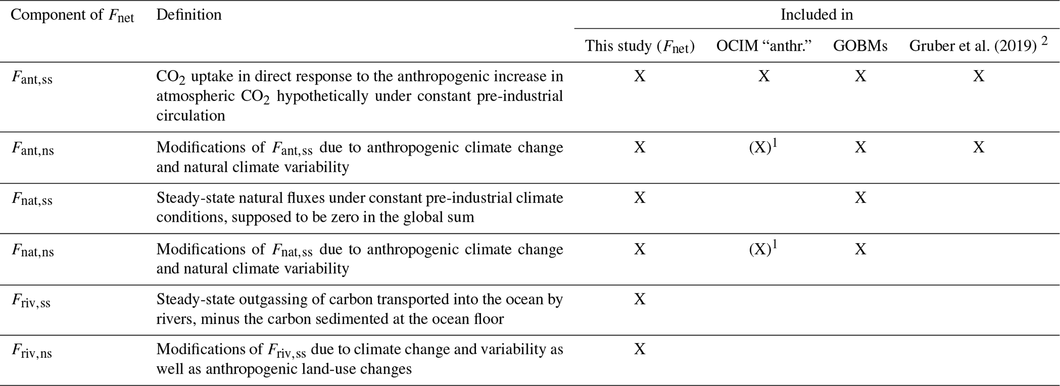
1 For a mean ocean circulation over the industrial era; i.e. the variations are due to temperature and gas transfer velocity variations only. 2 Mean 1994–2007 flux only.
From the increase in the anthropogenic carbon inventory in the ocean between the extensive ocean surveys in 1994 and 2007, Gruber et al. (2019) estimate an anthropogenic CO2 uptake of over the interjacent period, shown in Fig. A1 as a long-dashed line. This estimate conceptually differs from the hybrid mapping by the river-induced flux and the non-steady-state modifications Fnat,ns to the natural sea–air fluxes, while Fnat,ss is zero at the global scale (Table A1). The river-induced flux is very uncertain, with literature estimates ranging between (Jacobson et al., 2007) and (Resplandy et al., 2018), though the real uncertainty may be even larger. If the Gruber et al. (2019) estimate is shifted by a mid-range river-induced value of 0.62 PgC yr−1 (resulting in the dotted line), the base case value from the hybrid estimate is matched more closely. Nevertheless, given the uncertainty ranges of gas exchange, river-induced outgassing, and the Gruber et al. (2019) estimate, we cannot draw any conclusions from the remaining difference.
The CO2 flux difference between the hybrid estimate and the dotted line in Fig. A1 may also contain a contribution from systematic differences between pCO2 in the bulk ocean water (as typically measured at a few metres depth) and pCO2 at the diffusive surface layer (as relevant for gas exchange), arising due to systematic differences in water temperature and salinity (Woolf et al., 2016). Further, the cooler ocean skin temperature translates the atmospheric pCO2 to a different equilibrium DIC concentration than that implicitly calculated based on bulk temperature (Robertson and Watson, 1992). Watson et al. (2020) estimated that the sum of these two effects would shift pCO2-based estimates of the mean global CO2 flux by −0.8 to (stronger sink). So far, however, it is unclear how well the water temperature at the relevant vertical positions can actually be determined (an important source of uncertainty not included in the range of Watson et al., 2020) and how it varies in space and time. In any case, we note that our study mainly considers the variability in the flux, for which the effect of a time-constant correction as in Watson et al. (2020) would cancel out.
Figure A1 further shows the global fluxes simulated by a set of global ocean biogeochemical models (GOBMs) collated in the annual global carbon budget (Friedlingstein et al., 2020; mint green). Like OCIM or Gruber et al. (2019), the GOBMs' results do not include the river-induced flux component, but they do conceptually include the non-steady-state modification Fnat,ns of carbon uptake and natural carbon cycling (Table A1). The range of results covered by the GOBMs slightly exceeds the range of the hybrid estimates due to the gas exchange uncertainty. The medians of the GOBM ensemble and the pCO2 mapping ensemble differ by less than the mid-range river-induced value of 0.62 PgC yr−1.
A2 The secular sink trend (1960–2019)
Regarding the 1960–2019 secular sink trend, our estimate from the hybrid mapping (1) is not able to add much independent information and (2) even slightly overestimates this trend relative to OCIM used in the prior:
-
According to Fig. A2a, the 1960–2019 trend from the base case (solid blue bar) is quite similar to that of the base case prior (open grey bar). Among the uncertainty cases (hashed blue bars), the largest deviations are seen when mixed-layer depth is changed (MLDq2 and MLDx2); these deviations are in fact mostly inherited from their respective priors as well (not shown).
-
Figure A2a further reveals that the prior (open grey bar) has a slightly steeper trend than the OCIM estimate (magenta) even though the prior has been derived from OCIM (Sect. 2.1.3). This discrepancy arises because we are using OCIM's sea–air fluxes as a prior of the ocean-internal flux fint even though these two quantities differ by the carbon accumulation in the mixed layer. Since the carbon accumulation accelerates (following the accelerating increase in atmospheric pCO2), this leads to a difference not only in mean flux (Fig. A1) but also in trend. Due to the lack of information to correct the 1960–2019 secular trend from the pCO2 data as discussed under (1), this issue leads to an overestimation of the trend in the hybrid estimate compared to OCIM. Most GOBMs (mint green) simulate an even flatter 1960–2019 trend than OCIM.
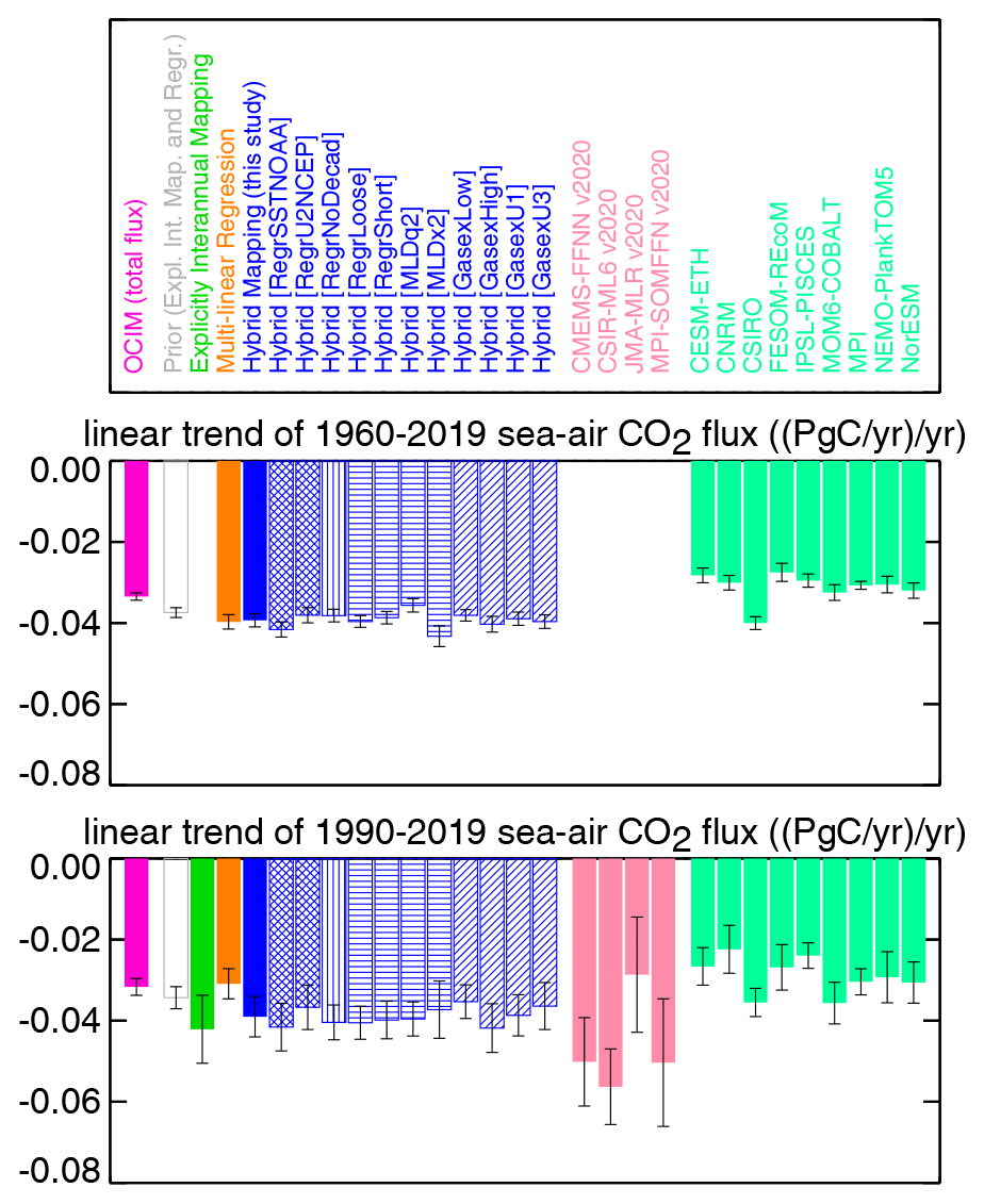
Figure A2Secular linear trend of the global sea–air CO2 flux over 1960–2019 (a) and over the more recent 1990–2019 period better constrained by pCO2 data (b), from the same estimates as in Fig. A1. The error bars give the formal error in the slope calculated from 5-year flux averages; i.e. they reflect the uncertainty due to the pentadal variability around the linear trend, thereby roughly taking into account the serial correlations of the flux, e.g. on the El Niño timescale.
Looking at the linear trend over the better-constrained, more recent period 1990–2019 (Fig. A2c), the estimate from the hybrid mapping becomes more independent from the prior. The pCO2-based hybrid estimates tend to show steeper trends than both OCIM and the GOBM simulations. Most other pCO2 mappings (salmon) estimate the trend to be even more negative than the hybrid mapping. However, given the substantial pentad-to-pentad variations in the global flux (as reflected in the error bars), it is not fully clear how well defined the trend over the 1990–2019 period actually is.
The level of constraint in the trend over the different periods is corroborated by the “zero-prior” mapping not using the secular trend from OCIM as a prior (Fig. A3). Even though the zero-prior explicitly interannual mapping (violet) and the explicitly interannual mapping (green) start from priors with very different secular trends (shown in dark and light grey, respectively), their estimated multi-decadal trends during the recent decades are still very close. In well-constrained regions like the tropical Pacific (bottom panel) they are practically identical, while some deviations occur in poorly constrained regions such as the Indian Ocean, adding up to the slight deviations in the global total flux (top). Only in the early decades where there are hardly any pCO2 data to constrain the estimates do the two mappings stick to the differing multi-decadal trends (and also to the year-to-year variations) of their respective priors.
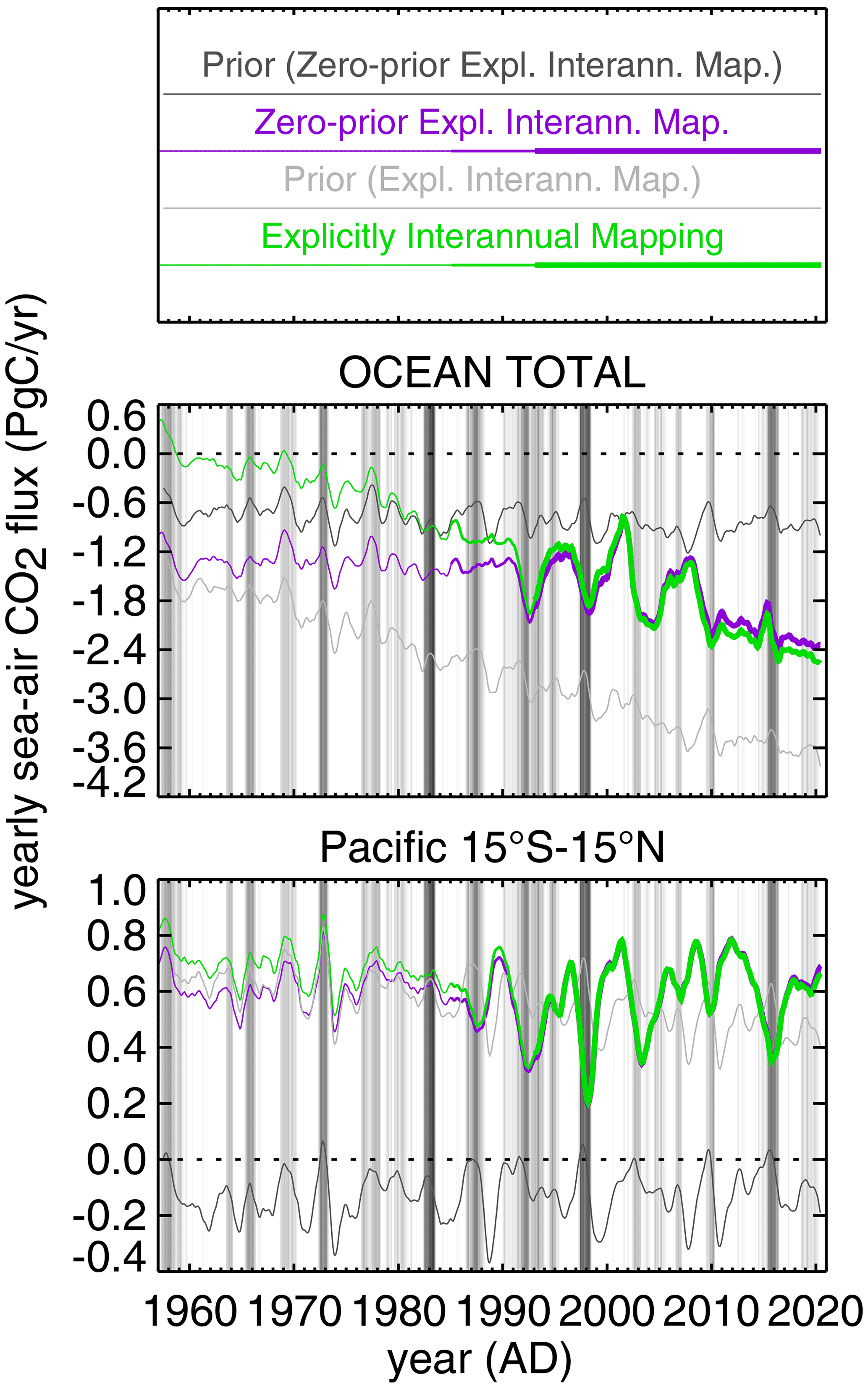
Figure A3Interannually filtered sea–air fluxes as in Fig. 6 (two example panels only) estimated by the zero-prior explicitly interannual pCO2 mapping (violet) and the explicitly interannual pCO2 mapping (green) as well as their respective priors (dark and light grey, respectively; note that the designation “zero-prior” refers to , while the a priori sea–air fluxes shown here are in fact non-zero owing to the rise in atmospheric CO2 and the variations in SST). The line width roughly distinguishes the early period with insufficient data constraint (thin) and the more recent period with better constraint (thick). Vertical background stripes as in Fig. 6.
As the better-constrained trend over the recent decades (after about 1992) is essentially the same as that in the prior of the explicitly interannual mapping, the flat multi-decadal trend of the zero-prior mapping in the early decades is very unlikely to be true. This illustrates that a prior with the correct secular trend (such as the OCIM result used here) is indeed needed to extrapolate the ocean CO2 sink into the data-poor first decades of our extended period of interest 1957–2020.
The sea–air CO2 flux estimates and the mapped pCO2 field of the hybrid mapping are available from http://www.bgc-jena.mpg.de/CarboScope/?ID=oc_v2021 (Jena CarboScope, 2021). Results of all other runs are available by replacing “oc_v2021” in this URL by the respective run IDs as given in Table 2. Auxiliary data can be made available upon request.
The supplement related to this article is available online at: https://doi.org/10.5194/bg-19-2627-2022-supplement.
CR designed and developed the pCO2 mapping algorithm, carried out the estimation runs, and drafted the paper. All other co-authors provided important expertise to interpret the results, reviewed the draft, and gave essential support to finalize the paper.
The contact author has declared that neither they nor their co-authors have any competing interests.
Publisher’s note: Copernicus Publications remains neutral with regard to jurisdictional claims in published maps and institutional affiliations.
We would like to thank all contributors to the SOCAT database, which is the basis of this work. We are grateful to Jim Orr for kindly providing the code of the mocsy package and helping us in its use. We would like to thank Rik Wanninkhof, Val Bennington, and Galen McKinley for helpful community comments and discussions on our manuscript.
Corinne Le Quéré received funding
from the Royal Society (grant no. RP/R1/191063)
and the Natural Environment Research Council Sonata project (NE/P021417/1).
Tim DeVries acknowledges support from NSF grant OCE-1948955.
The article processing charges for this open-access publication were covered by the Max Planck Society.
This paper was edited by Jack Middelburg and reviewed by two anonymous referees.
Atlas, R., Hoffman, R. N., Ardizzone, J., Leidner, S. M., Jusem, J. C., Smith, D. K., and Gombos, D.: A cross-calibrated, multi-platform ocean surface wind velocity product for meteorological and oceanographic applications, Bull. Am. Meteorol. Soc., 92, 157–174, 2011. a
Baker, D. F., Law, R. M., Gurney, K. R., Rayner, P., Peylin, P., Denning, A. S., Bousquet, P., Bruhwiler, L., Chen, Y.-H., Ciais, P., Fung, I. Y., Heimann, M., John, J., Maki, T., Maksyutov, S., Masarie, K., Prather, M., Pak, B., Taguchi, S., and Zhu, Z.: TransCom 3 inversion intercomparison: Impact of transport model errors on the interannual variability of regional CO2 fluxes, 1988–2003, Global Biogeochem. Cy., 20, GB1002, https://doi.org/10.1029/2004GB002439, 2006. a
Bakker, D. C. E., Pfeil, B., Landa, C. S., Metzl, N., O'Brien, K. M., Olsen, A., Smith, K., Cosca, C., Harasawa, S., Jones, S. D., Nakaoka, S.-I., Nojiri, Y., Schuster, U., Steinhoff, T., Sweeney, C., Takahashi, T., Tilbrook, B., Wada, C., Wanninkhof, R., Alin, S. R., Balestrini, C. F., Barbero, L., Bates, N. R., Bianchi, A. A., Bonou, F., Boutin, J., Bozec, Y., Burger, E. F., Cai, W.-J., Castle, R. D., Chen, L., Chierici, M., Currie, K., Evans, W., Featherstone, C., Feely, R. A., Fransson, A., Goyet, C., Greenwood, N., Gregor, L., Hankin, S., Hardman-Mountford, N. J., Harlay, J., Hauck, J., Hoppema, M., Humphreys, M. P., Hunt, C. W., Huss, B., Ibánhez, J. S. P., Johannessen, T., Keeling, R., Kitidis, V., Körtzinger, A., Kozyr, A., Krasakopoulou, E., Kuwata, A., Landschützer, P., Lauvset, S. K., Lefèvre, N., Lo Monaco, C., Manke, A., Mathis, J. T., Merlivat, L., Millero, F. J., Monteiro, P. M. S., Munro, D. R., Murata, A., Newberger, T., Omar, A. M., Ono, T., Paterson, K., Pearce, D., Pierrot, D., Robbins, L. L., Saito, S., Salisbury, J., Schlitzer, R., Schneider, B., Schweitzer, R., Sieger, R., Skjelvan, I., Sullivan, K. F., Sutherland, S. C., Sutton, A. J., Tadokoro, K., Telszewski, M., Tuma, M., van Heuven, S. M. A. C., Vandemark, D., Ward, B., Watson, A. J., and Xu, S.: A multi-decade record of high-quality fCO2 data in version 3 of the Surface Ocean CO2 Atlas (SOCAT), Earth Syst. Sci. Data, 8, 383–413, https://doi.org/10.5194/essd-8-383-2016, 2016. a, b, c, d, e, f
Bakker, D. C. E., Alin, S. R., Bates, N., Becker, M., Castaño-Primo, R., Cosca, C. E., Cronin, M., Kadono, K., Kozyr, A., Lauvset, S. K., Metzl, N., Munro, D. R., Nakaoka, S., O'Brien, K. M., Ólafsson, J., Olsen, A., Pfeil, B., Pierrot, D., Smith, K., Sutton, A. J., Takahashi, T., Tilbrook, B., Wanninkhof, R., Andersson, A., Atamanchuk, D., Benoit-Cattin, A., Bott, R., Burger, E. F., Cai, W.-J., Cantoni, C., Collins, A., Corredor, J. E., Cronin, M. F., Cross, J. N., Currie, K. I., De Carlo, E. H., DeGrandpre, M. D., Dietrich, C., Emerson, S., Enright, M. P., Evans, W., Feely, R. A., García-Ibáñez, M. I., Gkritzalis, T., Glockzin, M., Hales, B., Hartman, S. E., Hashida, G., Herndon, J., Howden, S. D., Humphreys, M. P., Hunt, C. W., Jones, S. D., Kim, S., Kitidis, V., Landa, C. S., Landschützer, P., Lebon, G. T., Lefèvre, N., Lo Monaco, C., Luchetta, A., Maenner Jones, S., Manke, A. B., Manzello, D., Mears, P., Mickett, J., Monacci, N. M., Morell, J. M., Musielewicz, S., Newberger, T., Newton, J., Noakes, S., Noh, J.-H., Nojiri, Y., Ohman, M., Ólafsdóttir, S. R., Omar, A. M., Ono, T., Osborne, J., Plueddemann, A. J., Rehder, G., Sabine, C. L., Salisbury, J. E., Schlitzer, R., Send, U., Skjelvan, I., Sparnocchia, S., Steinhoff, T., Sullivan, K. F., Sutherland, S. C., Sweeney, C., Tadokoro, K., Tanhua, T., Telszewski, M., Tomlinson, M., Tribollet, A., Trull, T., Vandemark, D., Wada, C., Wallace, D. W. R., Weller, R. A., and Woosley, R. J.: Surface Ocean CO2 Atlas Database Version 2020 (SOCATv2020) (NCEI Accession 0210711), NOAA National Centers for Environmental Information, https://doi.org/10.25921/4xkx-ss49, 2020. a, b
Bousquet, P., Peylin, P., Ciais, P., Le Quéré, C., Friedlingstein, P., and Tans, P. P.: Regional changes in carbon dioxide fluxes of land and oceans since 1980, Science, 290, 1342–1346, 2000. a
Carroll, D., Menemenlis, D., Adkins, J. F., Bowman, K. W., Brix, H., and Dutkiewicz, S., Fenty, I., Gierach, M. M., Hill, C., Jahn, O., Landschützer, P., Lauderdale, J. M., Liu, J., Manizza, M., Naviaux, J. D., Rödenbeck, C., Schimel, D. S., Van der Stocken, T., and Zhang, H.: The ECCO-Darwin data-assimilative global ocean biogeochemistry model: Estimates of seasonal to multidecadal surface ocean pCO2 and air-sea CO2 flux, J. Adv. Model. Earth Syst., 12, e2019MS001888, https://doi.org/10.1029/2019MS001888, 2020. a
Conkright, M., Locarnini, R. A., Garcia, H., O'Brien, T., Boyer, T., Stephens, C., and Antonov, J.: World Ocean Atlas 2001: Objective Analyses, Data Statistics, and Figures, CD-ROM Documentation. National Oceanographic Data Center, Silver Spring, MD, 17 pp., 2002. a
Conway, T., Tans, P., Waterman, L., Thoning, K., Kitzis, D., Masarie, K., and Zhang, N.: Evidence for interannual variability of the carbon cycle from the national oceanic and atmospheric administration climate monitoring and diagnostics laboratory global air sampling network, J. Geophys. Res., 99, 22831–22855, 1994. a
de Boyer Montégut, C., Madec, G., Fischer, A. S., Lazar, A., and Iudicone, D.: Mixed layer depth over the global ocean: an examination of profile data and a profile-based climatology, J. Geophys. Res., 109, C12003, https://doi.org/10.1029/2004JC002378, 2004. a
Denvil-Sommer, A., Gehlen, M., Vrac, M., and Mejia, C.: LSCE-FFNN-v1: a two-step neural network model for the reconstruction of surface ocean pCO2 over the global ocean, Geosci. Model Dev., 12, 2091–2105, https://doi.org/10.5194/gmd-12-2091-2019, 2019. a, b, c, d
DeVries, T.: Atmospheric CO2 and sea surface temperature variability cannot explain recent decadal variability of the ocean CO2 sink, Geophys. Res. Lett., 49, e2021GL096 018, https://doi.org/10.1029/2021GL096018, 2022. a, b, c, d
DeVries, T., Le Quéré, C., Andrews, O., Berthet, S., Hauck, J., Ilyina, T., Landschützer, P., Lenton, A., Lima, I. D., Nowick, M., Schwinger, J., and Séférian, R.: Decadal trends in the ocean carbon sink, P. Natl. Acad. Sci., 116, 11646–11651, https://doi.org/10.1073/pnas.1900371116, 2019. a
Feely, R. A., Wanninkhof, R., Takahashi, T., and Tans, P.: Influence of El Niño on the equatorial Pacific contribution to atmospheric CO2 accumulation, Nature, 398, 597–601, 1999. a
Francey, R., Steele, L., Spencer, D., Langenfelds, R., Law, R., Krummel, P., Fraser, P., Etheridge, D., Derek, N., Coram, S., Cooper, L., Allison, C., Porter, L., and Baly, S.: The CSIRO (Australia) measurement of greenhouse gases in the global atmosphere, Report of the 11th WMO/IAEA Meeting of Experts on Carbon Dioxide Concentration and Related Tracer Measurement Techniques, Tokyo, Japan, September 2001, edited by: Toru, S. and Kazuto, S., World Meteorological Organization Global Atmosphere Watch, 97–111, 2003. a
Friedlingstein, P., O'Sullivan, M., Jones, M. W., Andrew, R. M., Hauck, J., Olsen, A., Peters, G. P., Peters, W., Pongratz, J., Sitch, S., Le Quéré, C., Canadell, J. G., Ciais, P., Jackson, R. B., Alin, S., Aragão, L. E. O. C., Arneth, A., Arora, V., Bates, N. R., Becker, M., Benoit-Cattin, A., Bittig, H. C., Bopp, L., Bultan, S., Chandra, N., Chevallier, F., Chini, L. P., Evans, W., Florentie, L., Forster, P. M., Gasser, T., Gehlen, M., Gilfillan, D., Gkritzalis, T., Gregor, L., Gruber, N., Harris, I., Hartung, K., Haverd, V., Houghton, R. A., Ilyina, T., Jain, A. K., Joetzjer, E., Kadono, K., Kato, E., Kitidis, V., Korsbakken, J. I., Landschützer, P., Lefèvre, N., Lenton, A., Lienert, S., Liu, Z., Lombardozzi, D., Marland, G., Metzl, N., Munro, D. R., Nabel, J. E. M. S., Nakaoka, S.-I., Niwa, Y., O'Brien, K., Ono, T., Palmer, P. I., Pierrot, D., Poulter, B., Resplandy, L., Robertson, E., Rödenbeck, C., Schwinger, J., Séférian, R., Skjelvan, I., Smith, A. J. P., Sutton, A. J., Tanhua, T., Tans, P. P., Tian, H., Tilbrook, B., van der Werf, G., Vuichard, N., Walker, A. P., Wanninkhof, R., Watson, A. J., Willis, D., Wiltshire, A. J., Yuan, W., Yue, X., and Zaehle, S.: Global Carbon Budget 2020, Earth Syst. Sci. Data, 12, 3269–3340, https://doi.org/10.5194/essd-12-3269-2020, 2020. a, b, c, d
Garcia, H. E., Locarnini, R. A., Boyer, T. P., and Antonov, J. I.: World Ocean Atlas 2005, Vol. 4, Nutrients (phosphate, nitrate, silicate), edited by: Levitus, S., NOAA Atlas NESDIS 64, U.S. Government Printing Office, Washington, D.C., 396 pp., 2006. a
Gloege, L., McKinley, G. A., Landschützer, P., Fay, A. R., Frölicher, T. L., Fyfe, J. C., Ilyina, T., Jones, St., Lovenduski, N. S., Rodgers, K. B., Schlunegger, S., and Takano, Y.: Quantifying errors in observationally-based estimates of ocean carbon sink variability, Global Biogeochem. Cy., 35, e2020GB006788, https://doi.org/10.1029/2020GB006788, 2021. a
Good, S. A., Martin, M. J., and Rayner, N. A.: EN4: quality controlled ocean temperature and salinity profiles and monthly objective analyses with uncertainty estimates, J. Geophys. Res.-Ocean., 118, 6704–6716, https://doi.org/10.1002/2013JC009067, 2013. a, b
Gregor, L., Lebehot, A. D., Kok, S., and Scheel Monteiro, P. M.: A comparative assessment of the uncertainties of global surface ocean CO2 estimates using a machine-learning ensemble (CSIR-ML6 version 2019a) – have we hit the wall?, Geosci. Model Dev., 12, 5113–5136, https://doi.org/10.5194/gmd-12-5113-2019, 2019. a, b, c, d
Gruber, N., Clement, D., Carter, B. R., Feely, R. A., van Heuven, S., Hoppema, M., Ishii, M., Key, R. M., Kozyr, A., Lauvset, S. K., Lo Monaco, C., Mathis, J. T., Murata, A., Olsen, A., Perez, F. F., Sabine, C. L., Tanhua, T., and Wanninkhof, R.: The oceanic sink for anthropogenic CO2 from 1994 to 2007, Science, 363, 1193–1199, https://doi.org/10.1126/science.aau5153, 2019. a, b, c, d, e, f
Hauck, J., Völker, C., Wang, T., Hoppema, M., Losch, M., and Wolf-Gladrow, D. A.: Seasonally different carbon flux changes in the Southern Ocean in response to the southern annular mode, Global Biogeochem. Cy., 27, 1236–1245, https://doi.org/10.1002/2013GB004600, 2013. a, b, c
Hauck, J., Zeising, M., Quéré, C. L., Gruber, N., Bakker, D. C. E., Bopp, L., Chau, T. T. T., Gürses, Ö., Ilyina, T., Landschützer, P., Lenton, A., Resplandy, L., Rödenbeck, C., Schwinger, J., and Séférian, R.: Consistency and challenges in the ocean carbon sink estimate for the Global Carbon Budget, Front. Mar. Sci., 7, 571720, https://doi.org/10.3389/fmars.2020.571720, 2020. a, b
Hirt, C. and Rexer, M.: Earth2014: 1 arc-min shape, topography, bedrock and ice-sheet models – available as gridded data and degree-10,800 spherical harmonics, Int. J. Appl. Earth Obs., 39, 103–112, https://doi.org/10.1016/j.jag.2015.03.001, 2015. a
Huang, B., Thorne, P. W., Banzon, V. F., Boyer, T., Chepurin, G., Lawrimore, J. H., Menne, M. J., Smith, T. M., Vose, R. S., and Zhang, H.-M.: NOAA Extended Reconstructed Sea Surface Temperature (ERSST), Version 5., NOAA National Centers for Environmental Information, https://doi.org/10.7289/V5T72FNM, 2017 (ftp://ftp.cdc.noaa.gov/Datasets/noaa.ersst.v5/sst.mnmean.nc, last access: 26 June 2020). a
Iida, Y., Kojima, A., Takatani, Y., Nakano, T., Midorikawa, T., and Ishii, M.: Trends in pCO2 and sea-air CO2 flux over the global open oceans for the last two decades, J. Oceanogr., 71, 637–661, https://doi.org/10.1007/s10872-015-0306-4, 2015. a
Iida, Y., Takatani, Y., Kojima, A., and Ishii, M.: Global trends of ocean CO2 sink and ocean acidification: an observation-based reconstruction of surface ocean inorganic carbon variables, J. Oceanogr., 77, 323–358, https://doi.org/10.1007/s10872-020-00571-5, 2020. a, b, c
IPCC: Climate Change 2013: The Physical Science Basis, Contribution of Working Group I to the Fifth Assessment Report of the Intergovernmental Panel on Climate Change, edited by: Stocker, T. F., Qin, D., Plattner, G.-K., Tignor, M., Allen, S. K., Boschung, J., Nauels, A., Xia, Y., Bex, V., and Midgley, P. M., Cambridge University Press, Cambridge, United Kingdom and New York, NY, USA, 1535 pp., 2013. a
Jacobson, A. R., Fletcher, S. E. M., Gruber, N., Sarmiento, J. L., and Gloor, M.: A joint atmosphere-ocean inversion for surface fluxes of carbon dioxide: 2. Regional results, Global Biogeochem. Cy., 21, GB1020, https://doi.org/10.1029/2006GB002703, 2007. a, b
Jena CarboScope: Ocean-Atmosphere CO2 Exchange, http://www.bgc-jena.mpg.de/CarboScope/?ID=oc_v2021, last access: 26 August 2021. a
Jones, S. D., Quéré, C. L., Rödenbeck, C., Manning, A. C., and Olsen, A.: A statistical gap-filling method to interpolate global monthly surface ocean carbon dioxide data, J. Adv. Model. Earth Syst., 7, 1554–1575, https://doi.org/10.1002/2014MS000416, 2015. a
Kalnay, E., Kanamitsu, M., Kistler, R., Collins, W., Deaven, D., Gandin, L., Iredell, M., Saha, S., White, G., Woollen, J., Zhu, Y., Chelliah, M., Ebisuzaki, W., Higgins, W., Janowiak, J., Mo, K. C., Ropelewski, C., Wang, J., Leetmaa, A., Reynolds, R., Jenne, R., and Joseph, D.: The NCEP/NCAR 40-year reanalysis project, Bull. Am. Meteorol. Soc., 77, 437–471, 1996. a
Keeling, C. D.: The Influence of Mauna Loa Observatory on the Development of Atmospheric CO2 Research, in: Mauna Loa Observatory: a 20th anniversary report, edited by: Miller, J., Silver Spring, Md., U.S. Dept. of Commerce, National Oceanic and Atmospheric Administration, Environmental Research Laboratories, 35–54, 1978. a
Landschützer, P., Gruber, N., Bakker, D. C. E., Schuster, U., Nakaoka, S., Payne, M. R., Sasse, T. P., and Zeng, J.: A neural network-based estimate of the seasonal to inter-annual variability of the Atlantic Ocean carbon sink, Biogeosciences, 10, 7793–7815, https://doi.org/10.5194/bg-10-7793-2013, 2013. a, b, c, d
Landschützer, P., Gruber, N., and Bakker, D. C. E.: Decadal variations and trends of the global ocean carbon sink, Global Biogeochem. Cy., 30, 1396–1417, https://doi.org/10.1002/2015GB005359, 2016. a
Laws, E., Falkowski, P., Smith, W., Ducklow, H., and Mccarthy, J.: Temperature effects on export production in the open ocean, Global Biogeochem. Cy., 14, 1231–1246, https://doi.org/10.1029/1999GB001229, 2000. a
Lee, K., Tong, L. T., Millero, F. J., Sabine, C. L., Dickson, A. G., Goyet, C., Park, G.-H., Wanninkhof, R., Feely, R. A., and Key, R. M.: Global relationships of total alkalinity with salinity and temperature in surface waters of the world's oceans, Geophys. Res. Lett., 33, L19605, https://doi.org/10.1029/2006GL027207, 2006. a, b, c
Le Quéré, C., Orr, J. C., Monfray, P., and Aumont, O.: Interannual variability of the oceanic sink of CO2 from 1979 through 1997, Global Biogeochem. Cy., 14, 1247–1265, 2000. a
Le Quéré, C., Rödenbeck, C., Buitenhuis, E. T., Conway, T. J., Langenfelds, R., Gomez, A., Labuschagne, C., Ramonet, M., Nakazawa, T., Metzl, N., Gillett, N., and Heimann, M.: Saturation of the Southern Ocean CO2 Sink Due to Recent Climate Change, Science, 316, 1735–1738, https://doi.org/10.1126/science.1136188, 2007. a, b
Majkut, J. D., Sarmiento, J. L., and Rodgers, K. B.: A growing oceanic carbon uptake: Results from an inversion study of surface pCO2 data, Global Biogeochem. Cy., 28, 335–351, 2014. a
Maritorena, S., d'Andon, O. H. F., Mangin, A., and Siegel, D. A.: Merged satellite ocean color data products using a bio-optical model: Characteristics, benefits and issues, Remote Sens. Environ., 114, 1791–1804, https://doi.org/10.1016/j.rse.2010.04.002, 2010. a
Naegler, T.: Reconciliation of excess 14C-constrained global CO2 piston velocity estimates, Tellus B, 61, 372–384, 2009. a, b, c
Nakaoka, S., Telszewski, M., Nojiri, Y., Yasunaka, S., Miyazaki, C., Mukai, H., and Usui, N.: Estimating temporal and spatial variation of ocean surface pCO2 in the North Pacific using a self-organizing map neural network technique, Biogeosciences, 10, 6093–6106, https://doi.org/10.5194/bg-10-6093-2013, 2013. a
Newsam, G. N. and Enting, I. G.: Inverse problems in atmospheric constituent studies: I. Determination of surface sources under a diffusive transport approximation, Res. Meas. Ap., 4, 1037–1054, 1988. a
Orr, J. C. and Epitalon, J.-M.: Improved routines to model the ocean carbonate system: mocsy 2.0, Geosci. Model Dev., 8, 485–499, https://doi.org/10.5194/gmd-8-485-2015, 2015. a, b
Peylin, P., Law, R. M., Gurney, K. R., Chevallier, F., Jacobson, A. R., Maki, T., Niwa, Y., Patra, P. K., Peters, W., Rayner, P. J., Rödenbeck, C., van der Laan-Luijkx, I. T., and Zhang, X.: Global atmospheric carbon budget: results from an ensemble of atmospheric CO2 inversions, Biogeosciences, 10, 6699–6720, https://doi.org/10.5194/bg-10-6699-2013, 2013. a
Rayner, P., Enting, I., Francey, R., and Langenfelds, R.: Reconstructing the recent carbon cycle from atmospheric CO2, δ13CO2 and O2 N2 observations, Tellus B, 51, 213–232, 1999. a
Resplandy, L., Keeling, R. F., Rödenbeck, C., Stephens, B. B., Khatiwala, S., Rodgers, K. B., Long, M. C., Bopp, L., and Tans, P. P.: Revision of global carbon fluxes based on a reassessment of oceanic and riverine carbon transport, Nat. Geosci., 11, 504–509, https://doi.org/10.1038/s41561-018-0151-3, 2018. a, b
Robertson, J. E. and Watson, A. J.: Thermal skin effect of the surface ocean and its implications for CO2 uptake, Nature, 358, 738–740, 1992. a
Rödenbeck, C.: Estimating CO2 sources and sinks from atmospheric mixing ratio measurements using a global inversion of atmospheric transport, Tech. Rep. 6, Max Planck Institute for Biogeochemistry, Jena, Germany, 2005. a
Rödenbeck, C., Houweling, S., Gloor, M., and Heimann, M.: CO2 flux history 1982–2001 inferred from atmospheric data using a global inversion of atmospheric transport, Atmos. Chem. Phys., 3, 1919–1964, https://doi.org/10.5194/acp-3-1919-2003, 2003. a
Rödenbeck, C., Keeling, R. F., Bakker, D. C. E., Metzl, N., Olsen, A., Sabine, C., and Heimann, M.: Global surface-ocean pCO2 and sea–air CO2 flux variability from an observation-driven ocean mixed-layer scheme, Ocean Sci., 9, 193–216, https://doi.org/10.5194/os-9-193-2013, 2013. a, b, c, d, e, f, g, h, i, j, k, l, m, n, o, p, q, r, s
Rödenbeck, C., Bakker, D. C. E., Metzl, N., Olsen, A., Sabine, C., Cassar, N., Reum, F., Keeling, R. F., and Heimann, M.: Interannual sea–air CO2 flux variability from an observation-driven ocean mixed-layer scheme, Biogeosciences, 11, 4599–4613, https://doi.org/10.5194/bg-11-4599-2014, 2014. a, b, c, d
Rödenbeck, C., Bakker, D. C. E., Gruber, N., Iida, Y., Jacobson, A. R., Jones, S., Landschützer, P., Metzl, N., Nakaoka, S., Olsen, A., Park, G.-H., Peylin, P., Rodgers, K. B., Sasse, T. P., Schuster, U., Shutler, J. D., Valsala, V., Wanninkhof, R., and Zeng, J.: Data-based estimates of the ocean carbon sink variability – first results of the Surface Ocean pCO2 Mapping intercomparison (SOCOM), Biogeosciences, 12, 7251–7278, https://doi.org/10.5194/bg-12-7251-2015, 2015. a
Rödenbeck, C., Zaehle, S., Keeling, R., and Heimann, M.: History of El Nino impacts on the global carbon cycle 1957–2016: A quantification from atmospheric CO2 data, Philos. T. R. Soc. B, 373, 20170303, https://doi.org/10.1098/rstb.2017.0303, 2018a. a
Rödenbeck, C., Zaehle, S., Keeling, R., and Heimann, M.: How does the terrestrial carbon exchange respond to inter-annual climatic variations? A quantification based on atmospheric CO2 data, Biogeosciences, 15, 2481–2498, https://doi.org/10.5194/bg-15-2481-2018, 2018b. a, b
Sarmiento, J. L. and Gruber, N.: Ocean Biogeochemical Dynamics, Princeton Univ. Press, 2006. a
Takahashi, T., Sutherland, S. C., Wanninkhof, R., Sweeney, C., Feely, R. A., Chipman, D. W., Hales, B., Friederich, G., Chavez, F., Sabine, C., Watson, A., Bakker, D. C. E., Schuster, U., Metzl, N., Yoshikawa-Inoue, H., Ishii, M., Midorikawa, T., Nojiri, Y., Kortzinger, A., Steinhoff, T., Hoppema, M., Olafsson, J., Arnarson, T. S., Tillbrook, B., Johannessen, T., Olsen, A., Bellerby, R., Wong, C. S., Delille, B., Bates, N. R., and de Baar, H. J. W.: Climatological mean and decadal change in surface ocean pCO2 and net sea-air CO2 flux over the global oceans, Deep-Sea Res. Pt. II, 56, 554–577, 2009. a
Thacker, W. C.: Regression-based estimates of the rate of accumulation of anthropogenic CO2 in the ocean: A fresh look, Mar. Chem., 132/133, 44–55, https://doi.org/10.1016/j.marchem.2012.02.004, 2012. a
Titchner, H. A. and Rayner, N. A.: The Met Office Hadley Centre sea ice and sea surface temperature data set, version 2: 1. Sea ice concentrations, J. Geophys. Res.-Atmos., 119, 2864–2889, https://doi.org/10.1002/2013JD020316, 2014. a, b
Tsujino, H., Urakawa, S., Nakano, H., Small, R. J., Kim, W. M., Yeager, S. G., Danabasoglu, G., Suzuki, T., Bamber, J. L., Bentsen, M., Boening, C., Bozec, A., Chassignet, E., Curchitser, E., Dias, F. B., Durack, P. J., Griffies, S. M., Harada, Y., Ilicak, M., Josey, S., Kobayashi, C., Kobayashi, S., Komuro, Y., Large, W. G., Le Sommer, J., Marsland, S., Masina, S., Scheinert, M., Tomita, H., Valdivieso, M., and Yamazaki, D.: input4MIPs.CMIP6.OMIP.MRI, https://doi.org/10.22033/ESGF/input4MIPs.10460, 2018. a, b
Valsala, K. V. and Maksyutov, S.: Simulation and assimilation of global ocean pCO2 and air-sea CO2 fluxes using ship observations of surface ocean pCO2 in a simplified Biogeochemical offline model, Tellus B, 62, 821–840, 2010. a
Wanninkhof, R.: Relationship between wind speed and gas exchange over the ocean, J. Geophys. Res.-Ocean., 97, 7373–7382, 1992. a
Watson, A. J., Schuster, U., Bakker, D. C. E., Bates, N. R., Corbiére, A., González-Dávila, M., Friedrich, T., Hauck, J., Heinze, C., Johannessen, T., Körtzinger, A., Metzl, N., Olafsson, J., Olsen, A., Oschlies, A., Padin, X. A., Pfeil, B., Santana-Casiano, J. M., Steinhoff, T., Telszewski, M., Rios, A. F., Wallace, D. W. R., and Wanninkhof, R.: Tracking the Variable North Atlantic Sink for Atmospheric CO2, Science, 326, 1391–1393, 2009. a
Watson, A. J., Schuster, U., Shutler, J. D., Holding, T., Ashton, I. G. C., Landschützer, P., Woolf, D. K., and Goddijn-Murphy, L.: Revised estimates of ocean-atmosphere CO2 flux are consistent with ocean carbon inventory, Nat. Commun., 11, 4422, https://doi.org/10.1038/s41467-020-18203-3, 2020. a, b, c
Weiss, R.: Carbon dioxide in water and seawater: the solubility of a non-ideal gas, Mar. Chem., 2, 203–205, 1974. a
Wolter, K. and Timlin, M.: Monitoring ENSO in COADS with a seasonally adjusted principal component index, Proc. of the 17th Climate Diagnostics Workshop, Norman, OK, NOAA/N MC/CAC, NSSL, Oklahoma Clim. Survey, CIMMS and the School of Meteor., Univ. of Oklahoma, 52–57, 1993. a, b, c
Woolf, D. K., Land, P. E., Shutler, J. D., Goddijn-Murphy, L. M., and Donlon, C. J.: On the calculation of air-sea fluxes of CO2 in the presence of temperature and salinity gradients, J. Geophys. Res.-Ocean., 121, 1229–1248, 2016. a
Yu, L. and Weller, R. A.: Objectively Analyzed air-sea heat Fluxes (OAFlux) for the global oceans, Bull. Am. Meteorol. Soc., 88, 527–539, 2007. a
Zeng, J., Nojiri, Y., Nakaoka, S., Nakajima, H., and Shirai, T.: Surface ocean CO2 in 1990–2011 modelled using a feed-forward neural network, Geosci. Data J., 2, 47–51, 2015. a
- Abstract
- Introduction
- Method
- Results
- Discussion: robustness of the multi-linear regression
- Conclusions
- Appendix A: The global ocean carbon sink estimated by the hybrid mapping
- Data availability
- Author contributions
- Competing interests
- Disclaimer
- Acknowledgements
- Financial support
- Review statement
- References
- Supplement