the Creative Commons Attribution 4.0 License.
the Creative Commons Attribution 4.0 License.
 | 15 Sep 2022
Observation-constrained estimates of the global ocean carbon sink from Earth system models
Thomas L. Frölicher
Fortunat Joos
The ocean slows global warming by currently taking up around one-quarter of all human-made CO2 emissions. However, estimates of the ocean anthropogenic carbon uptake vary across various observation-based and model-based approaches. Here, we show that the global ocean anthropogenic carbon sink simulated by Earth system models can be constrained by two physical parameters, the present-day sea surface salinity in the subtropical–polar frontal zone in the Southern Ocean and the strength of the Atlantic Meridional Overturning Circulation, and one biogeochemical parameter, the Revelle factor of the global surface ocean. The Revelle factor quantifies the chemical capacity of seawater to take up carbon for a given increase in atmospheric CO2. By exploiting this three-dimensional emergent constraint with observations, we provide a new model- and observation-based estimate of the past, present, and future global ocean anthropogenic carbon sink and show that the ocean carbon sink is 9 %–11 % larger than previously estimated. Furthermore, the constraint reduces uncertainties of the past and present global ocean anthropogenic carbon sink by 42 %–59 % and the future sink by 32 %–62 % depending on the scenario, allowing for a better understanding of the global carbon cycle and better-targeted climate and ocean policies. Our constrained results are in good agreement with the anthropogenic carbon air–sea flux estimates over the last three decades based on observations of the CO2 partial pressure at the ocean surface in the Global Carbon Budget 2021, and they suggest that existing hindcast ocean-only model simulations underestimate the global ocean anthropogenic carbon sink. The key parameters identified here for the ocean anthropogenic carbon sink should be quantified when presenting simulated ocean anthropogenic carbon uptake as in the Global Carbon Budget and be used to adjust these simulated estimates if necessary. The larger ocean carbon sink results in enhanced ocean acidification over the 21st century, which further threatens marine ecosystems by reducing the water volume that is projected to be undersaturated towards aragonite by around 3.7×10⁶–7.4×10⁶ km3 more than originally projected.
- Article
(3905 KB) - Full-text XML
- BibTeX
- EndNote


The emissions of anthropogenic carbon (Cant) since the beginning of industrialization through fossil-fuel burning, cement production, and land-use change have altered the global carbon cycle and climate (Friedlingstein et al., 2022). Around 40 % of the additional carbon since 1850 has accumulated in the atmosphere, where it represents the main anthropogenic greenhouse gas (IPCC, 2021). More than half of the emitted Cant has been taken up by the land biosphere (∼ 30 %) and the ocean (∼ 25 %) (Friedlingstein et al., 2022). The remaining ∼ 5 % is the budget imbalance, a mismatch between carbon emissions and sink estimates which cannot be explained yet (Friedlingstein et al., 2022). By each taking up around a quarter of the Cant emissions, the land biosphere and ocean sinks slow down global warming and climate change.
The ocean Cant sink is defined here as a combination of the uptake of newly emitted carbon and the change in the natural carbon inventory in the ocean due to changes in temperatures, winds, and the freshwater cycle caused by climate change (Joos et al., 1999; Frölicher and Joos, 2010; McNeil and Matear, 2013). The uptake rate of Cant on sub-millennial timescales is mainly determined by the ocean circulation and carbonate chemistry and only partly by biology (Sarmiento et al., 1998; Joos et al., 1999; Caldeira and Duffy, 2000; Sabine et al., 2004) despite the overall importance of marine biology for natural carbon fluxes (Falkowski et al., 1998; Steinacher et al., 2010). The rate-limiting process of Cant uptake is the circulation that transports surface waters with high Cant concentrations into the deeper ocean and allows waters with low or no Cant concentrations to upwell back to the ocean surface. The largest part of this ocean upwelling occurs in the Southern Ocean where strong westerlies drive northward Ekman transport of surface waters, which are then replaced by older, deeper water masses (Marshall and Speer, 2012; Talley, 2013; Morrison et al., 2015). These predominantly northward flowing waters take up Cant from the atmosphere and are eventually transferred to mode and intermediate waters that sink back into the ocean interior (Marshall and Speer, 2012; Talley, 2013). This overturning makes the Southern Ocean the largest marine Cant sink (∼ 40 % of global ocean Cant uptake) (Caldeira and Duffy, 2000; Mikaloff Fletcher et al., 2006; Frölicher et al., 2015; Terhaar et al., 2021b). Another region of large uptake rates is the North Atlantic (Caldeira and Duffy, 2000; Mikaloff Fletcher et al., 2006), where the Atlantic Meridional Overturning Circulation (AMOC) transports surface waters with high Cant (Pérez et al., 2013) and subsurface waters with low Cant concentrations northward (Ridge and McKinley, 2020). The subsurface waters outcrop in the subpolar North Atlantic where they take up Cant from the atmosphere (Ridge and McKinley, 2020). These high Cant waters are then ventilated by the AMOC into the deep ocean where the Cant is efficiently stored (Joos et al., 1999; Winton et al., 2013).
While the circulation determines the volume that is transported into the deeper ocean, the Revelle factor (Revelle and Suess, 1957; Sabine et al., 2004) determines the concentration of Cant in these water masses. The Revelle factor describes the biogeochemical capacity of the ocean to take up Cant. This biogeochemical capacity is strongly dependent on the amount of carbonate ions in the ocean that react with CO2 and H2O to form bicarbonate ions (Egleston et al., 2010; Goodwin et al., 2009; Revelle and Suess, 1957). The more CO2 is transferred via this reaction to bicarbonate ions, the more CO2 can be taken up again from the atmosphere. The available amount of carbonate ions for this reaction depends sensitively on the difference between ocean alkalinity and dissolved inorganic carbon (CT) (Fig. A2 in Appendix A) (Egleston et al., 2010; Goodwin et al., 2009; Revelle and Suess, 1957), highlighting the importance of alkalinity for the global ocean carbon uptake (Middelburg et al., 2020). As the buffer factor influences the Cant uptake, it also exerts a strong control on the transient climate response, i.e., the warming per cumulative CO2 emissions (Katavouta et al., 2018; Rodgers et al., 2020).
In addition to slowing global warming, the Cant uptake by the ocean also causes ocean acidification (Orr et al., 2005; Gattuso and Hansson, 2011; Kwiatkowski et al., 2020), i.e., a decline in ocean pH and carbonate ion concentrations. The decline in carbonate ion concentrations has negative effects on the growth and survival of many marine species, especially on calcifying organisms whose shells and skeletons are made up of calcium carbonate minerals (Orr et al., 2005; Fabry et al., 2008; Kroeker et al., 2010, 2013; Doney et al., 2020). Calcium carbonate minerals in the ocean exist mainly in the metastable forms of aragonite and high-magnesium calcite and the more stable form calcite. The stability of calcium carbonate minerals is described by their saturation states (Ω), which describe the product of the concentrations of calcium ([Ca2+]) and carbonate ions ([CO]) divided by their product in equilibrium. Reductions of saturation states of aragonite (Ωarag) and calcite (Ωcalc) have been shown to negatively impact organisms and ecosystems (Langdon and Atkinson, 2005; Kroeker et al., 2010; Bednaršek et al., 2014; Albright et al., 2016). Once saturation states drop below one, the water is undersaturated and actively corrosive towards the respective mineral form.
Accurately quantifying the ocean anthropogenic carbon sink is thus of crucial importance for understanding and quantifying the carbon cycle, global warming, and climate change, as well as ocean acidification. A better knowledge of the size of the historical and future ocean carbon sink and reduced uncertainties will hence not only lead to an improved understanding of the overall carbon cycle and global climate change (IPCC, 2021) but also allow targeted climate and ocean policies (IPCC, 2022). One of the key tools to assess the past, present, and future ocean carbon sink is Earth system models (ESMs). However, the simulated ocean Cant sink varies across the different ESMs (Frölicher et al., 2015; Wang et al., 2016; Bronselaer et al., 2017; Terhaar et al., 2021b), and the model differences grow over time; i.e., ESMs that simulate a small ocean Cant uptake over the last decades also simulate a small uptake over the 21st century (Fig. 1b) (Wang et al., 2016). Therefore, a better knowledge of the ocean Cant sink in the last decades would be one possibility to reduce uncertainties in the simulated ocean carbon from 1850 to 2100.

Figure 1Simulated ocean anthropogenic carbon uptake from Earth system models. (a) Simulated annual mean air–sea Cant fluxes from 17 CMIP6 Earth system models from 1990 to 2020 before (orange line) and after the constraint is applied (blue line). After 2014, results from SSP5-8.5 were chosen as this is the only SSP for which each model provided results, and differences in atmospheric CO2 mixing ratios in SSP5-8.5 (Meinshausen et al., 2020) are small compared to observations until 2020 (maximum difference of 2.5 ppm in 2020) (NOAA/GML, 2022). In addition, mean air–sea Cant fluxes based on multiple observation-based estimates (solid black line) and hindcast simulations (dashed black line) from the Global Carbon Budget 2021 (Friedlingstein et al., 2022) are shown. For readability, the uncertainties of these estimates (on average 0.24 Pg C yr−1 for observation-based estimates and 0.28 Pg C yr−1 for hindcast simulations) are not shown in the figure. (b) Simulated cumulative ocean Cant uptake since 1765 for the historic period until 2014 (17 ESMs) and for the future from 2015 to 2100 under SSP1-2.6 (blue, 14 ESMs), SSP2-4.5 (orange, 16 ESMs), and SSP5-8.5 (red, 17 ESMs). Thin lines show the results from each individual ESM, the dashed lines the multi-model mean, the solid lines the constrained estimate, and the shading the uncertainty around the constrained estimate. Furthermore, the observation-based ocean Cant inventory estimate in 2010 from Khatiwala et al. (2013) is shown. As ESM simulations in CMIP6 start in 1850, the air–sea Cant fluxes were corrected upwards for the late starting date in the constrained estimate following Bronselaer et al. (2017) (see Appendix A, Sect. A1).
The large background concentration of CT in the ocean and the vast ocean volume make it difficult to directly observe the relatively small anthropogenic perturbations in the ocean interior. Therefore, different methods have been developed to estimate the accumulation of Cant in the ocean (Khatiwala et al., 2013), such as the ΔC* method (Gruber et al., 1996; Sabine et al., 2004) or the transient time distribution method (Hall et al., 2002) based on observations of inert tracers, like CFCs. These estimates result in an estimated ocean Cant inventory in 2010 of 155 ± 31 Pg C (Khatiwala et al., 2013) (Fig. 1b, Table 1) but do not or only partly include climate-driven changes in CT.
Further development of the ΔC* method into the eMLR(C*) method (Clement and Gruber, 2018) and more observations through new techniques, such as Biogeochemical-Argo (BGC-Argo) floats (Claustre et al., 2020), and more research cruises (Lauvset et al., 2021) will allow the increase in marine Cant to be quantified on shorter timescales and with reduced uncertainty. The increase in Cant from 1994 to 2007 by the eMLR(C*) method is 34 ± 4 Pg C (12 % uncertainty, Table 1) (Gruber et al., 2019a), again not accounting for potential climate-driven changes in CT. In addition to interior Cant estimates, surface ocean observations of the partial pressure of CO2 (pCO2) and new statistical methods, such as neural networks (Landschützer et al., 2016), have led to a variety of observation-based estimates of the air–sea CO2 flux (Rödenbeck et al., 2014; Zeng et al., 2014; Landschützer et al., 2016; Gregor et al., 2019; Watson et al., 2020; Iida et al., 2021; Gregor and Gruber, 2021; Chau et al., 2022). When subtracting the pre-industrial outflux of CO2 due to riverine carbon fluxes (Sarmiento and Sundquist, 1992; Aumont et al., 2001; Jacobson et al., 2007; Resplandy et al., 2018; Lacroix et al., 2020; Regnier et al., 2022) from these air–sea CO2 flux estimates, the global ocean Cant uptake can be derived (Friedlingstein et al., 2022), resulting in an estimated ocean Cant uptake from 1994 to 2007 of 29 ± 4 Pg C (14 % uncertainty, Table 1).
The difference of 5 Pg C between the interior and surface ocean mean estimates was attributed to outgassing of ocean CO2 caused by a changing climate and climate variability (Gruber et al., 2019a). However, simulations from ESMs of the sixth phase of the Coupled Model Intercomparison Project (CMIP6) estimate the climate-driven and externally forced climate-variability-driven air–sea CO2 flux from 1994 to 2007 to be only −1.6 ± 0.5 Pg C (Table A3). When averaging over an ensemble of ESMs, forced variability (e.g., due to the volcanic eruptions or varying emissions of CO2 and other radiative agents) is still preserved. However, unforced interannual-to-decadal variability is largely removed when averaging over an ensemble of ESMs. Although comparisons suggest that the ocean Cant uptake was low compared to atmospheric CO2 in the 1990s and high in the 2000s (Rödenbeck et al., 2013, 2022), a comparison of different Cant uptake estimates for different decadal-scale periods does not reveal any clear variability-related deviation for the 1994–2007 period (IPCC, 2021, AR6 WGI, chap. 5, Fig. 5.8; Canadell et al., 2021). Overall, uncertainties remain at present too large for any quantitative conclusions, but it seems unlikely that unforced variability causes an air–sea CO2 flux of −3.4 Pg C (difference between −5 Pg C from Gruber et al. (2019a) and −1.6 Pg C from ESMs), twice as large as the simulated flux from forced variability and climate change. It hence remains a challenge to derive the total ocean Cant sink from interior estimates that do not account for climate-driven changes in CT.
An alternative way of estimating the strength of the ocean carbon sink is the use of global ocean biogeochemical models forced with atmospheric reanalysis data (Sarmiento et al., 1992; Friedlingstein et al., 2022). From 1994 to 2007, the ocean biogeochemical hindcast models that participated in the Global Carbon Budget 2021 (Friedlingstein et al., 2022) simulate a Cant uptake of 26 ± 3 Pg C (Table 1). This estimate is 3 Pg C below the surface observation-based estimate, and the difference increases further after 2010 (Fig. 1a). Compared to the interior ocean Cant estimate, the simulated uptake by these hindcast models is 3–6 Pg C (10 %–19 %) smaller depending on the correction term that is used for climate-change-induced outgassing of natural CO2. Such differences between observation-based and simulated ocean Cant uptake could be explained regionally by systematic biases in models (Goris et al., 2018; Terhaar et al., 2020a, 2021a, b), as well as data sparsity (Bushinsky et al., 2019; Gloege et al., 2021).
Overall, the difference between ocean hindcast models, observation-based CO2 flux estimates, and interior ocean Cant estimates, as well as the uncertainties in the climate-driven change in CT and pre-industrial outgassing, indicate that uncertainties of the ocean Cant sink over the last decades remain substantial. The uncertainty of the Cant sink appears larger than the uncertainty typically given for an individual estimate of the Cant sink from a specific data product.
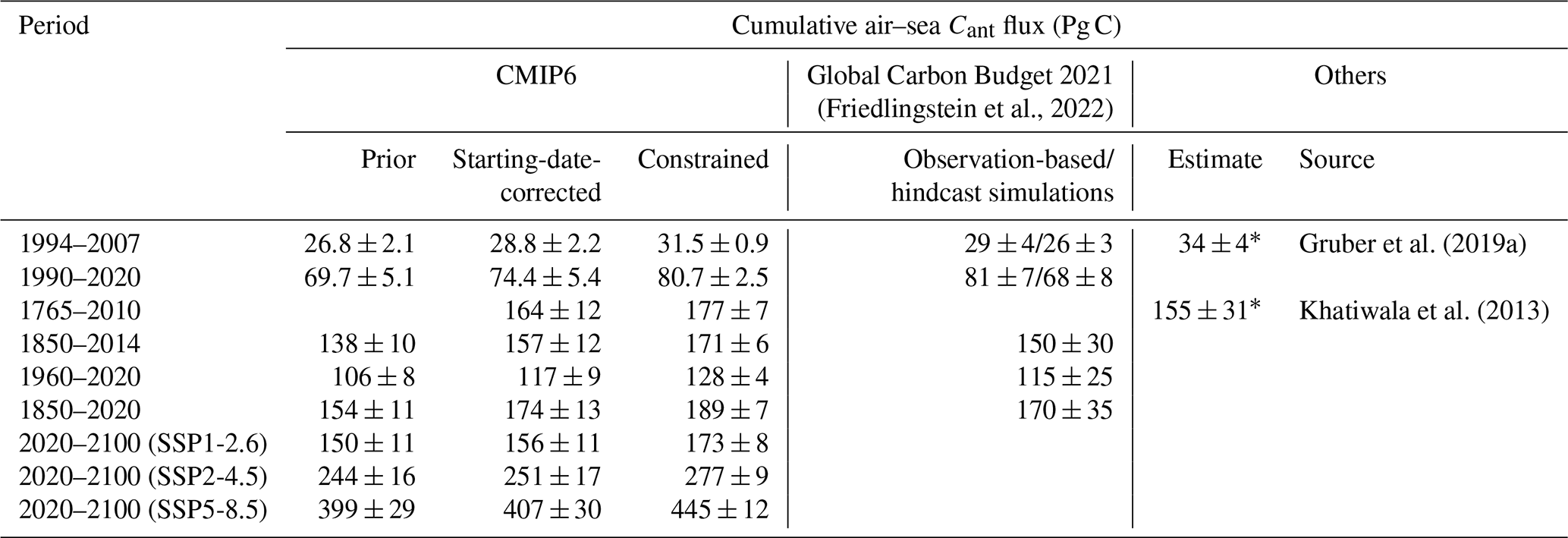
Table 1Global ocean air–sea Cant flux estimates based on 17 ESMs from CMIP6 before and after being starting-date-corrected and constrained, as well as previous estimates over different time periods. Prior uncertainty is the multi-model standard deviation. The uncertainty of the starting-date-corrected values also includes the uncertainty from that correction. The constrained uncertainty is a combination of the starting date correction, the multi-model standard deviation after the constraint is applied, and the uncertainty from the correction itself (see Sects. 3.1 and A1). Uncertainties from the decadal variability on shorter timescales, e.g., for 1994–2007, are not included. The star indicates estimates that do not account for climate-driven changes in the ocean carbon sink.
Another way to constrain the past, present, and future global ocean anthropogenic carbon sink is the use of process-based emergent constraints (Orr, 2002) that identify a relationship across an ensemble of ESMs between a relatively uncertain variable, such as the Cant uptake in the Southern Ocean, and a variable that can be observed with a relatively small uncertainty, such as the sea surface salinity in the subtropical–polar frontal zone in the Southern Ocean. The identified relationship is then combined with observations, in this example the sea surface salinity, to better estimate the uncertain variable, here the Cant uptake in the Southern Ocean (Terhaar et al., 2021b). Such relationships must be explainable by an underlying mechanism (Hall et al., 2019); i.e., higher sea surface salinity in the frontal zone leads to denser sea surface waters and stronger mode and intermediate water formation, which enhances the transport of Cant from the ocean surface to the ocean interior and allows hence for more Cant uptake. In recent years, process-based emergent constraints have successfully reduced uncertainties in simulated processes across ensembles of ESMs (Orr, 2002; Matsumoto et al., 2004; Wenzel et al., 2014; Kwiatkowski et al., 2017; Goris et al., 2018; Eyring et al., 2019; Hall et al., 2019; Terhaar et al., 2020a, 2021a, b; Bourgeois et al., 2022). In the ocean, for example, a bias towards smaller Cant uptake was identified in the Southern Ocean (Terhaar et al., 2021b). Similarly, ESMs from CMIP5 were shown to underestimate the future uptake of Cant in the North Atlantic due to smaller than observed sequestration of Cant into the deeper ocean (Goris et al., 2018). However, the relatively uncertain observation-based estimates of Cant sequestration (see section above) did not allow Goris et al. (2018) to reduce uncertainties. Similarly, the Cant uptake in the tropical Pacific Ocean across ESMs could be reduced with observations of the local surface ocean carbonate ion concentrations (Vaittinada Ayar et al., 2022), which is anti-correlated to the Revelle factor. Despite a better understanding of the regional Cant uptake, uncertainties of the global ocean Cant sink have not been reduced yet.
Here, we identify a mechanistic constraint for the global ocean Cant sink across 17 ESMs from CMIP6 (Table A1 in Appendix A). We demonstrate that a linear combination of three observable quantities, (1) the sea surface salinity in the subtropical–polar frontal zone in the Southern Ocean, (2) the strength of the AMOC at 26.5∘ N, and (3) the globally averaged surface ocean Revelle factor, can successfully predict the strength of the global ocean Cant sink across the CMIP6 ESMs (r2 of 0.87 for the global ocean Cant uptake from 1994 to 2007). The sea surface salinity in the subtropical–polar frontal zone in the Southern Ocean and the AMOC determine the strength of the two most important regions of mode, intermediate, and deep-water formation (Goris et al., 2018, 2022; Terhaar et al., 2021b). In addition, the Revelle factor accounts for biases in the biogeochemical buffer capacity of the ocean, i.e., the relative increase in ocean CT for a given relative increase in ocean pCO2 (Revelle and Suess, 1957). As the Revelle factor quantifies relative increases in ocean CT, the increase in surface ocean Cant depends on the Revelle factor and the natural surface ocean CT. Therefore, the Revelle factor in the ESMs was adjusted for model biases in natural surface ocean CT (see Sect. A1). Compared to observations, CMIP6 models represent the observation-based average strength of the AMOC from 2004 to 2020 (16.91 ± 0.49 Sv) (McCarthy et al., 2020) right but have a large inter-model spread (16.91 ± 3.00 Sv), underestimate the observed inter-frontal sea surface salinity (34.07 ± 0.02) and have a large inter-model spread (33.89 ± 0.13), and overestimate the surface-averaged Revelle factor that was derived by GLODAPv2 (10.45 ± 0.01) by 0.24 (10.73 ± 0.24) with the largest Revelle factor biases in the main Cant uptake regions (Fig. 2). The underestimation of the CT-adjusted Revelle factor by the ESM ensemble is mainly due to a bias towards concentrations of surface ocean carbonate ion concentrations that are smaller than the observed concentrations (Sarmiento et al., 1995), caused by a simulated difference of surface ocean alkalinity and CT that is smaller than the observed difference (Fig. A2).
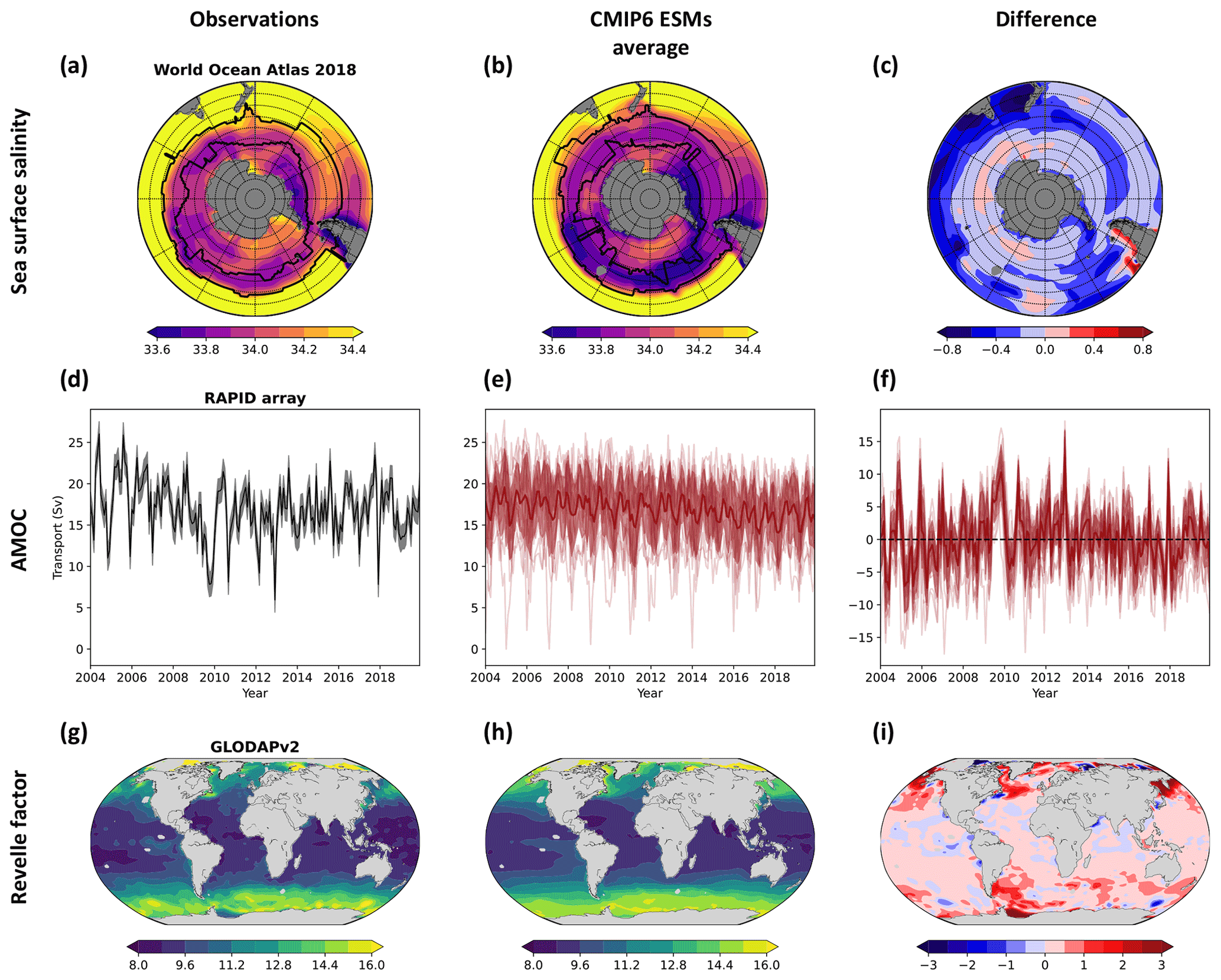
Figure 2Sea surface salinity in the Southern Ocean, the Atlantic Meridional Overturning Circulation, and the Revelle factor at the ocean surface from observations and Earth system models. Annual mean sea surface salinity from the (a) World Ocean Atlas 2018 (Zweng et al., 2018; Locarnini et al., 2018), (b) 17 Earth system models from CMIP6 from 1995 to 2014, and (c) the difference between both. The black lines in (a, b) indicate the annual mean positions of the polar and subtropical fronts. The strength of the monthly-averaged Atlantic Meridional Overturning Circulation, here defined as the maximum of the streamfunction at 26.5∘ N, from 2004 to 2020 (d) as observed by the RAPID array (McCarthy et al., 2020), (e) as simulated by 17 Earth system models from CMIP6, and (f) the difference between both. Each model simulation is shown in (e) and (f) as a thin red line, the multi-model average is shown as a thick red line, and the multi-model standard deviation is shown as red shading. The annual mean sea surface Revelle factor calculated with mocsy2.0 (Orr and Epitalon, 2015) from (g) gridded GLODAPv2 observations that are normalized to the year 2002 (Lauvset et al., 2016), from (h) output of 17 Earth system model simulations from CMIP6 in 2002 and adjusted for biases in the surface ocean CT (see Sect. A1), and (i) their difference.
3.1 Applying the constraint and uncertainty estimation
For the three-dimensional emergent constraint, multi-linear regression was used. First, it was assumed that the ocean Cant uptake for every model M () can be approximated by a linear combination of the inter-frontal sea surface salinity in the Southern Ocean in model M (SSS), the AMOC strength in model M (AMOCM), and the globally averaged surface ocean Revelle factor in model M (Revelle):
The parameters a, b, and c are scaling parameters of the three predictor variables, d is the y intercept, and ε describes the residual between the predicted Cant flux by this multi-linear regression model and the simulated Cant uptake by model M. The free parameters a, b, c, and d were fitted based on the simulated inter-frontal sea surface salinity in the Southern Ocean, AMOC, Revelle factor, and Cant uptake. The three predictors are not statistically correlated (r2=0.00 for salinity and AMOC, r2=0.03 for Revelle factor and AMOC, and r2=0.10 for salinity and Revelle factor) and can hence be used in a multi-linear regression.
The constrained Cant flux is estimated by replacing the simulated inter-frontal sea surface salinity in the Southern Ocean, AMOC, and Revelle factor by the observed ones and by setting ε to zero. As the Revelle factor describes the inverse of the ocean capacity to take up Cant from the atmosphere, Eq. (1) should in principal be used with . However, using facilitates understanding and the presentation of the results and only introduces maximum errors of around 0.1 % for the Revelle factor adjustment for the models that simulate the largest deviations from the observed Revelle factor. To estimate the uncertainty, all model results were first corrected for their biases in the three predictor variables; i.e., if a model has a salinity that is 0.2 smaller than the observed salinity, the simulated Cant uptake by this model is increased by a⋅0.2. The same correction is made for the other two predictor variables (Fig. 3). If the three predictor variables were predicting the Cant flux perfectly, the bias-corrected Cant uptake from all models would be the same. The remaining inter-model standard deviation therefore represents the uncertainty from the multi-linear regression model due to other factors that influence the ocean Cant uptake. The second part of the uncertainty originates from the uncertainty in the observations of the predictor variables that influences the magnitude of the correction. This uncertainty () is calculated as follows:
with , ΔAMOCobs, and being the uncertainty of the three observed predictor variables. Eventually, the overall uncertainty of this constrained Cant flux is estimated as the square root of the sum of the products of the square of both uncertainties.
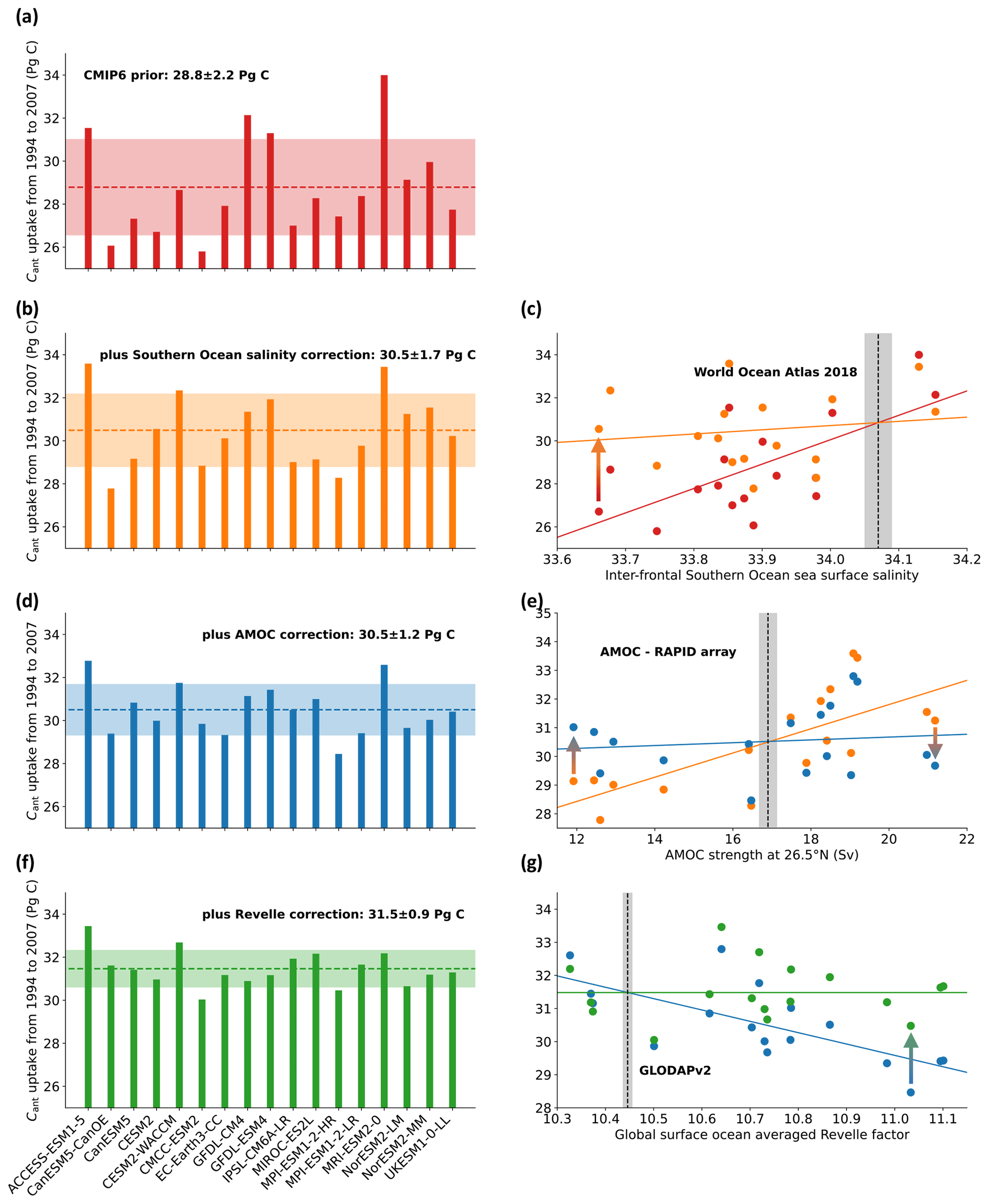
Figure 3Global ocean anthropogenic carbon simulated by Earth system models from CMIP6 corrected for biases in sea surface salinity in the Southern Ocean, the Atlantic Meridional Overturning Circulation, and the Revelle factor. (a) Global ocean anthropogenic carbon (Cant) uptake from 1994 to 2007 as simulated by 17 ESMs from CMIP6 and corrected for the late starting date (Bronselaer et al., 2017). For each ESM, one ensemble member was used, as the difference between ensemble members has been shown to be small compared to the inter-model differences (Terhaar et al., 2020a, 2021b). In the years 1994 and 2007, only half of the annual Cant uptake was accounted for to make it comparable to interior ocean estimates that compare changes in Cant from mid-1994 to mid-2007 and not from the start of 1994 to the end of 2007 (Gruber et al., 2019a). (b) Cant uptake after correcting the simulated Cant uptake from (a) for biases in the Southern Ocean sea surface salinity (Terhaar et al., 2021b) from (c). The dots in (c) represent individual models before (red) and after (orange) the sea surface salinity correction. (d) Cant uptake after correcting sea-surface-salinity-corrected Cant uptake from (b) for biases in the Atlantic Meridional Overturning Circulation from (e). The dots in (e) represent individual models before (orange) and after (blue) the Atlantic Meridional Overturning Circulation correction. (f) Cant uptake after correcting the sea-surface-salinity- and AMOC-corrected Cant uptake from (d) for biases in the global ocean surface Revelle factor from (g). The dots in (g) represent individual models before (blue) and after (green) the Revelle factor correction. The simulated Revelle factor by the ESMs was adjusted for biases in the surface ocean CT (see Sect. A1). The dashed colored lines in (a), (b), (d), and (f) show the multi-model mean, and the shading shows the uncertainty, which is a combination of the multi-model standard deviation after correction and the uncertainty of the correction factor due to the uncertainty of the observational constraint (see Sect. A1). The dashed black lines in (c), (e), and (g) show the observations from the World Ocean Atlas 2018 (Zweng et al., 2018; Locarnini et al., 2018), the RAPID array (McCarthy et al., 2020), and GLODAPv2 (Lauvset et al., 2016) with their uncertainties as grey shading, the colored lines show linear fits, and the arrows illustrate the correction for individual models.
3.2 Exploiting the constraint with observations
By exploiting this multi-variable emergent constraint with observations, the simulated Cant uptake by ESMs from 1994 to 2007 increases from 28.8 ± 2.2 to 31.5 ± 0.9 Pg C (Figs. 1 and 3, Tables 1 and A2). Biases in the Southern Ocean salinity are responsible for around 60 % of the bias in the global ocean Cant uptake in the CMIP6 models, while the bias in the Revelle factor explains the remaining 40 % (Fig. 3). The AMOC, whose multi-model mean in ESMs is similar to observations, does not change the central Cant uptake estimate but allows uncertainties (Fig. 3) to be reduced. The constrained Cant uptake of 31.5 ± 0.9 Pg C is 0.9 Pg C smaller than the interior ocean Cant estimate of 34 ± 4 Pg C based on observations (Gruber et al., 2019a) when subtracting the multi-model mean climate-driven CO2 flux estimate from the CMIP6 models of 1.6 Pg C (Table A3). This difference of 0.9 Pg C is smaller than the uncertainties. Furthermore, the constrained Cant uptake of 31.5 ± 0.9 Pg C is 2.5 Pg C larger than the observation-based air–sea Cant flux estimates from 1994 to 2007 of 29 ± 4 Pg C from the Global Carbon Budget 2021 (Table 1), but both estimates agree within the uncertainties. When comparing a short period, for example the years after 2013, the observation-based air–sea Cant flux estimates can deviate from the constrained CMIP6 ESM estimates (Fig. 1) due to unforced climate-variability-driven CO2 flux. Thus, the small difference between observation-based ocean Cant uptake estimates from 1994 to 2007 and the results provided here may not exist over a longer period of time and be caused by a different timing and magnitude of decadal variabilities in ESMs and the real world (Landschützer et al., 2016; Gruber et al., 2019b; Bennington et al., 2022), as well as uncertainties in the observation-based products (Bushinsky et al., 2019; Gloege et al., 2021, 2022). Indeed, when the entire period for which observation-based air–sea Cant flux estimates from the Global Carbon Budget are available (1990–2020), the constrained estimate of the ocean Cant sink based on ESMs (80.7 ± 2.5 Pg C) is very similar to the observation-based estimate from surface ocean pCO2 observations (81 ± 7 Pg C) (Table 1).
The good agreement between the air–sea Cant flux estimates from ESMs and surface ocean pCO2 observations in combination with interior ocean Cant of a similar magnitude suggests that the air–sea Cant flux from hindcast simulations over the last three decades (68 ± 8 Pg C) and possibly also over the 1994–2007 period (26 ± 3 Pg C) underestimates the ocean Cant uptake (Table 1). Therefore, the Global Carbon Budget 2021 estimate of the ocean Cant uptake over the last decades, which is an average of the estimate of Cant uptake from observation-based methods and hindcast models, should be corrected upwards. Reasons for this underestimation may be an underestimation of the AMOC or the Southern Ocean inter-frontal sea surface salinity, an overestimation of the Revelle factor, a small ensemble of models (8 models) that are biased towards low uptake models, very short spin-up times (Séférian et al., 2016), neglecting the water vapor pressure when calculating the local pCO2 in each ocean grid cell (Hauck et al., 2020) as is done in CMIP models (Orr et al., 2017), or different pre-industrial atmospheric CO2 mixing ratios (Bronselaer et al., 2017; Friedlingstein et al., 2022). However, even after correcting these hindcast simulations upwards by employing the emergent constraint identified here, their corrected estimate may remain below the CMIP-derived estimate for the period from 1994 to 2017 due to the historical decadal variations in the Cant uptake that is not represented with the same phasing in fully coupled ESMs (Landschützer et al., 2016; Gruber et al., 2019b; Bennington et al., 2022). A detailed analysis by the individual modeling teams would be necessary to identify the reason for underestimation in the individual hindcast models, as the output is not openly available.
Over the historical period from 1850 to 2020, the constraint identified here increases the simulated ocean Cant uptake by 15 Pg C (r2=0.80) from 174 ± 13 to 189 ± 7 Pg C (Table 1). The constrained estimate of the Cant agrees within the uncertainties of the estimate from the Global Carbon Budget for the same period (170 ± 35 Pg C) (Friedlingstein et al., 2022), which is a combination of prognostic approaches until 1959 (Khatiwala et al., 2013; DeVries, 2014), and ocean hindcast simulations and observation-based CO2 flux products from 1960 to 2020 (Friedlingstein et al., 2022). However, our new estimate is 19 Pg C larger and could explain around three-quarters of the budget imbalance (BIM) between global CO2 emissions and sinks over the period 1850 to 2020 (25 Pg C) (Friedlingstein et al., 2022) and contribute to answering an important outstanding question in the carbon cycle community.
Overall, this new estimate of the ocean Cant uptake, based on ESMs and constrained by observations, presents an independent and new estimate of the past and present ocean Cant uptake that is around 10 % larger and 42 %–59 % less uncertain than the multi-model average and its standard deviation, respectively. The lower bound of the uncertainty correction is for the past ocean Cant uptake since 1765 in which the late starting date correction introduces an uncertainty that cannot be reduced without running the simulations from 1765 onwards. Towards the end of the 20th century, the uncertainty from this correction becomes smaller so that the emergent constraint can reduce uncertainties by almost 60 %.
3.2.1 Southern Ocean
While the constraints were applied globally, they are also applicable regionally as shown for the inter-frontal sea surface salinity in the Southern Ocean (Terhaar et al., 2021b). Here, we update the regional constraint in the Southern Ocean with the now additionally available ESMs and extend the constraint by adding the basin-wide-averaged Revelle factor in the Southern Ocean as a second variable. For the period from 1765 to 2005, the simulated multi-model mean air–sea Cant flux that is adjusted for the late starting date is 63.5 ± 6.1 Pg C. Please note that the numbers here are for fluxes from 1765 to 2005 and are not the same as in Terhaar et al. (2021b), where fluxes from 1850 to 2005 were reported. The two-dimensional constraint shows a higher correlation coefficient (r2=0.70) than the one-dimensional constraint when only the inter-frontal sea surface salinity is used as a predictor (r2=0.62). Slight differences to Terhaar et al. (2021b) exist due to the additional ESMs that are by now available. When exploiting this relationship with observations of the Southern Ocean Revelle factor (12.19 ± 0.01) and the sea surface salinity, the best estimate of the cumulative air–sea Cant flux from 1765 to 2005 in the Southern Ocean increases to 72.0 ± 3.4 Pg C. In comparison, observation-based estimates for the same period report 69.6 ± 12.4 Pg C (Mikaloff Fletcher et al., 2006) and 72.1 ± 12.6 Pg C (Gerber et al., 2009). The constraint thus reduces the uncertainty not only globally but also in the Southern Ocean by 44 %.
3.2.2 Atlantic Ocean
As for the Southern Ocean, we also apply a two-dimensional constraint to the Atlantic Ocean, using the AMOC and the basin-wide-averaged surface ocean Revelle factor in the North Atlantic as predictors. The unconstrained cumulative air–sea Cant flux from 1765 to 2005 in the North Atlantic adjusted for the late starting date is 21.9 ± 3.3 Pg C. For this period, the two-dimensional constraint results in a relationship with a correlation coefficient of 0.57. If only the AMOC had been used, the correlation factor would have been 0.49. When exploiting this relationship with observations of the North Atlantic Revelle factor and AMOC, the best estimate of the cumulative air–sea Cant flux from 1765 to 2005 in the Atlantic Ocean increases to 22.7 ± 2.2 Pg C. In comparison, observation-based estimates are 20.4 ± 4.9 Pg C (Mikaloff Fletcher et al., 2006) and 20.4 ± 6.5 Pg C (Gerber et al., 2009). The constrained and unconstrained estimates are both above the observation-based estimates but within the uncertainties. The constrained estimate is even higher than the unconstrained one but only by 0.8 Pg C, and its uncertainty is reduced by 33 %.
As the present and future Cant uptake are strongly correlated across ESMs, the relationship identified here can also be used to constrain future projections of the global ocean Cant uptake. The global ocean Cant uptake from 2020 to 2100 increases from 156 ± 11 to 173 ± 8 Pg C (r2=0.56) under the high-mitigation, low-emission Shared Socioeconomic Pathway 1-2.6 (SSP1-2.6) that likely allows us to keep global warming below 2 ∘C (O'Neill et al., 2016; Riahi et al., 2017), from 251 ± 17 to 277 ± 9 Pg C (r2=0.74) under the middle-of-the-road SSP2-4.5, and from 407 ± 30 Pg C to 445 ± 12 Pg C (r2=0.87) under the high-emission, no-mitigation SSP5-8.5 (Fig. 1b). Overall, the future ocean Cant uptake in CMIP6 models is thus 9 %–11 % larger than simulated by ESMs and 32 %–62 % less uncertain depending on the future scenario. The correlation coefficient and hence the uncertainty reduction reduces – but remains still large – when atmospheric CO2 stops increasing (SSP1-2.6, SSP2-4.5). Larger uncertainties for stabilization than for near-exponential growth scenarios are expected, as the reversal of the atmospheric CO2 growth rate will exert a stronger external impact on the magnitude of the ocean carbon sink (McKinley et al., 2020).
The increase in projected uptake of Cant also increases the estimate of future ocean acidification rate. For ocean ecosystems, the threshold for water masses to become undersaturated towards specific calcium carbonate minerals (Ω=1) is of critical importance (Orr et al., 2005; Fabry et al., 2008; Doney et al., 2020), although negative effects for some calcifying organisms can already be observed at saturation states above one (Ries et al., 2009), and some calcifying organisms can even live in undersaturated waters (Lebrato et al., 2016). Over the 21st century, the volume of water masses in the global ocean that remain supersaturated towards the meta-stable calcium carbonate mineral aragonite is projected to decrease in CMIP6 from 283×106 km3 in 2002 (based on GLODAPv2 observations; Lauvset et al., 2016) to 194×106 ± 6×10⁶ km3 under SSP1-2.6, to 143×106 ± 4×10⁶ km3 under SSP2-4.5, and to 97×106 ± 4×10⁶ km3 under SSP5-8.5. The constraint reduces these estimates to 186×106 ± 5×10⁶, 138×106 ± 2×10⁶, and 93×106 ± 2×10⁶ km3, respectively (r2 = 0.31–0.69), resulting in an additional decrease in the available habitat for calcifying organisms of 3.7×10⁶–7.4×10⁶ km3 depending on the scenario. This additionally projected habitat loss is mainly located in the mesopelagic layer between 200 and 1000 m and thus affects organisms that live there permanently or temporarily during diel vertical migration (Behrenfeld et al., 2019). The additionally undersaturated volume corresponds to an area of 1.6–3.1 times the area of the Mediterranean Sea whose mesopelagic layer would be additionally undersaturated towards aragonite. However, the global character of the constraint and the uncertainty of the interior distribution of Cant do not allow us to localize these areas.
Emergent constraints across large datasets such as an ensemble of ESMs with hundreds of variables can always be found and might not necessarily be reliable and robust (Caldwell et al., 2014; Brient, 2020; Sanderson et al., 2021; Williamson et al., 2021). To test the robustness of emergent constraints, three criteria were proposed (Hall et al., 2019). The constraint must be relying on a well-understood mechanism, that mechanism must be reliable, and the constraint must be validated in an independent model ensemble.
Here, the well-understood mechanisms are the fundamental ocean biogeochemical properties such as the Revelle factor (Revelle and Suess, 1957), as well as the Southern Ocean and North Atlantic large-scale ocean circulation features that are known to be the determining factors for the ocean ventilation (Marshall and Speer, 2012; Talley, 2013; Buckley and Marshall, 2016). For the Southern Ocean, the verification of the link between sea surface salinity and Cant uptake was previously done by linking the sea surface salinity to the density and to the volume of intermediate and mode waters in each model. Furthermore, the robustness of the constraint was tested against changes in the definition of the inter-frontal zone (Terhaar et al., 2021b). In addition, other potential predictors were tested, such as the magnitude and seasonal cycle of sea-ice extent, wind curl, and the mixed layer depth, as well as upwelling strength of circumpolar deep waters. All these variables are known to influence air–sea gas exchange, freshwater fluxes, and circulation and, in turn, salinity and Cant uptake. However, none of these factors alone explains biases in the surface salinity and Cant uptake in the Southern Ocean. Therefore, the sea surface salinity that emerges as a result of all these individual processes represents, so far, the best variable in terms of mechanistic explanation and observational uncertainty to bias-correct models for Southern Ocean Cant uptake. Further evidence for the underlying mechanism of the relationship between Southern Ocean sea surface salinity and Cant uptake was provided by a later study that analyzed explicitly the stratification in the water column (Bourgeois et al., 2022). Here, we further showed that the Southern Ocean Cant uptake constrained by the Revelle factor and the inter-frontal sea surface salinity compares much better to observation-based estimates than the unconstrained estimate, further corroborating the identified regional constraint and mechanism (Sect. 3.2.1).
Similarly, it was shown that the transport of Cant by the AMOC is crucial for the Cant uptake in the North Atlantic (Winton et al., 2013; Goris et al., 2018; Brown et al., 2021). As the AMOC is predominantly observed at 26.5∘ N, a change to the definition is not possible. Instead, we replaced the AMOC as a predictor by another indicator for deep-water formation, namely the area of waters in the North Atlantic below which the water column is weakly stratified (see Sect. A1 and Table A4) (Hess, 2022). The results remain almost unchanged, indicating the robustness of the constraint and that the AMOC is indeed a good indicator for the stability of the water column in the North Atlantic and the associated deep-water formation. As for the Southern Ocean, we also made a regional two-dimensional constraint using the AMOC and the regional Revelle factor and compared it to observation-based Cant flux estimates. The good relationship between the AMOC and the North Atlantic Cant uptake improves the confidence in the AMOC as a valid predictor.
Eventually, we also tested the robustness of the biogeochemical predictor by varying the definition of the Revelle factor. First, the Revelle factor was only calculated north of 45∘ N and south of 45∘ S, assuming that the high-latitude regions are responsible for the largest Cant uptake, and second, the global Revelle factor was calculated by weighting the Revelle factor in each cell by the multi-model mean cumulative Cant uptake from 1850 to 2100 in that cell so that the Revelle factor in cells with larger uptake is more strongly weighted. Under both definitions, the results remain almost unchanged (Table A4). Furthermore, the Revelle factor has been shown here to improve the Cant uptake in the Atlantic and Southern Ocean and has been earlier shown to determine the Cant uptake in the tropical Pacific Ocean (Vaittinada Ayar et al., 2022), suggesting that the Revelle factor is a robust predictor of global and regional ocean Cant uptake.
To provide further indication of the importance of the AMOC and the Southern Ocean surface salinity and the three-dimensional constraint in general, we have compared simulated CFC-11, provided by 10 ESMs from CMIP6, with observed CFC-11 from GLODAPv2.2021 (Lauvset et al., 2021) (Sect. A4) and also compared the interior ocean distribution of Cant with observation-based estimates (Sabine et al., 2004; Gruber et al., 2019a) (Sect. A5). The comparison of CFCs demonstrates the importance of the AMOC for the ventilation of the North Atlantic, as ESMs with a low AMOC underestimate the observed subsurface CFC-11 concentrations in the North Atlantic. Similarly, ESMs with a small inter-frontal Southern Ocean surface salinity underestimate observed subsurface (below 200 m) CFC-11 concentrations in the Southern Hemisphere. In addition to the evaluation with observations of CFC, the comparison of the interior ocean Cant distribution demonstrates first that the ESMs on average represent the observation-based distributions within the margins of error (Tables A5 and A6). Only in the Southern Hemisphere does the ESM average remain below, as expected due to the average ESM bias towards inter-frontal sea surface salinities that are too low compared to observed ones, less formation of mode and intermediate waters, and hence relatively little storage of Cant in the Southern Hemisphere. When using the model that represents best the three predictors, GFDL-ESM4 (Geophysical Fluid Dynamics Laboratory ESM4; Dunne et al., 2020; Stock et al., 2020), the comparison to observation-based interior ocean Cant distribution becomes almost identical (Tables A7 and A8), suggesting that a better representation of these parameters indeed improves the simulation of Cant uptake and its distribution in the ocean interior.
To validate the constraint identified here in another model ensemble, we used all six ESMs of the CMIP5 ensemble that provided all necessary output variables (Table A1). As these six ESMs are not sufficient to robustly fit a function with four unknown parameters, we applied the predicted relationship by the CMIP6 models to the CMIP5 models and evaluated how well this relationship allows the simulated historical Cant uptake to be predicted by these models. The CMIP6-derived relationship allows us to predict the simulated Cant uptake with an accuracy of 3 % (± 5 Pg C) for the period from 1850 to 2014 and with an accuracy of 4 % (± 1.3 Pg C) for the period from 1994 to 2007 (Fig. A5). The largest uncertainty stems from the NorESM2-ME (Norwegian Earth System Model version 2) model, which simulates a historical AMOC strength of ∼ 30 Sv, almost twice as large as the observed AMOC strength and ∼ 9 Sv larger than all other CMIP6 ESMs over which the relationship was fitted. For such strong deviations from the observations and other ESMs, the linear relationship might not be applicable anymore. However, despite one out of six ESMs from CMIP5 having a particularly high AMOC, the relationship identified here still allows us to predict the simulated Cant uptake with small uncertainties and hence confirms its applicability.
Despite this robustness, emergent constraints are, by definition, always relying on the existing ESMs and on the processes that are represented by these ESMs. If certain processes are not implemented or implemented in the same way across all ESMs, biases over the entire model ensemble can occur that cannot be corrected by an emergent constraint (Sanderson et al., 2021). Possible non-represented processes in our case are, among others, changing freshwater input from the Greenland and Antarctic ice sheet that may impact the freshwater cycle and circulation in the Southern Ocean or the AMOC, as well as changes in riverine input of carbon over time. However, the expected effect of ice melt on sea surface salinity in the Southern Ocean and on the AMOC is small compared to the model spread (Bakker et al., 2016; Terhaar et al., 2021b), at least on the timescales considered here. Changing riverine carbon fluxes could, however, have a larger effect. So far, only one CMIP6 ESM, the CNRM-ESM2-1 (Séférian et al., 2019), has dynamic carbon riverine delivery that changes with global warming. In this model, carbon riverine delivery increases over the 20th century so that the interior ocean change in Cant in 2000 is around 19 Pg C smaller than the air–sea Cant uptake (Fig. A4). The situation reverses at the beginning of the 21st century so that riverine carbon delivery increases, and the interior ocean change in Cant becomes up to 60 Pg C larger than the air–sea Cant uptake. As such, riverine carbon delivery has the potential to enhance or decrease the ocean Cant inventory in addition to air–sea Cant uptake. This would also question the comparability of Cant inventory and air–sea Cant uptake estimates. However, the present state of the ESMs does not allow a quantitative assessment of this process, and future research is needed.
In addition, parametrizations of non-represented processes such as mesoscale and sub-mesoscale circulation features like small-scale eddies may lead to biases in the model ensemble. For individual models, it has been shown that changes in horizontal resolution and hence a more explicitly simulated circulation change the model physics and biogeochemistry and hence also the ocean carbon and heat uptake (Lachkar et al., 2007, 2009; Dufour et al., 2015; Griffies et al., 2015). However, an increase in resolution does not necessarily lead to improved simulations, and the changes in oceanic Cant uptake may be lower or higher, depending on the model applied. When increasing the NEMO (Nucleus for European Modelling of the Ocean) ocean model from a non-eddying version (2∘ horizontal resolution) to an eddying version (0.5∘), Lachkar et al. (2009) find a decrease in the sea surface salinity of around 0.1 at the Southern Ocean surface that brings the model further away from the observed salinity, a decrease in the volume of Antarctic intermediate water, and a decrease in the Southern Ocean uptake of CFC and hence likely also of Cant. This example corroborates the underlying mechanism of the emergent constraint in the Southern Ocean that higher sea surface salinity directly affects the formation of Antarctic intermediate water and the uptake of Cant. Another example can be found within the ESM ensemble of CMIP6. The MPI-ESM-1-2-HR and MPI-ESM-1-2-LR have a horizontal resolution of 0.4 and 1.5∘, respectively, but the same underlying ocean model. The high-resolution version has an inter-frontal salinity of 33.98, a Southern Ocean surface Revelle factor of 12.82, and a Southern Ocean Cant uptake from 1850 to 2005 of 56.4 Pg C. The coarser-resolution version has an inter-frontal sea surface salinity of 33.92, a Southern Ocean surface Revelle factor of 12.89, and a Southern Ocean Cant uptake of 58.0 Pg C. These differences are much smaller than the inter-model differences (33.66–34.15 for salinity, 12.14–13.11 for the Revelle factor, and 48.8–71.1 Pg C for the Southern Ocean Cant uptake) that result from different ocean circulation and biogeochemical models, sea-ice models, and atmospheric and land biosphere models, as well as the coupling between these models. These examples show that higher resolution does not necessarily lead to better results, affecting potentially the predictor and the predicted variable in the same way, and that differences in the underlying model components and spin-up and initialization strategies lead so far to much larger differences between ESMs than resolution does (Séférian et al., 2020). As long as simulations with higher resolution, which are also spun-up over hundreds of years (Séférian et al., 2016), are not yet available, and potentially important processes such as changing riverine fluxes and freshwater from land ice are not included, it remains speculative if higher resolution would lead to a reduction in inter-model uncertainty or even a better representation of the observations. Moreover, the relationships identified here that are based on the current understanding of physical and biogeochemical oceanography and that were tested for robustness in several ways may likely also exist across ensembles of eddy-resolving models.
The three-dimensional emergent constraint identified here reveals a bias towards an insufficient Cant uptake by the CMIP6 ESM ensemble, reduces uncertainties of the global ocean Cant sink, and leads to an enhanced process understanding of the Cant uptake in ESMs. The constraint was tested for robustness in multiple ways and across different model ensembles. It was evaluated regionally and globally against CFC measurements, against estimates of the interior ocean Cant accumulation, and against observation-based estimates of the air–sea CO2 flux globally and regionally. The constraint demonstrates that the global ocean Cant uptake can be estimated from three observable variables, the salinity in the subtropical–polar frontal zone in the Southern Ocean, the Atlantic Meridional Overturning Circulation, and the global surface ocean Revelle factor. The uncertainties of the regional ocean Cant uptake estimates in the Atlantic and Southern Ocean can also be reduced with the respective regional predictors. Improved or continuing observations of these quantities (Lauvset et al., 2016; Zweng et al., 2018; Locarnini et al., 2018; Claustre et al., 2020; McCarthy et al., 2020) and their representation and evaluation in ESMs and ocean models should therefore be of priority in the next years and decades. Although biogeochemical variables were tuned or calibrated in more ESMs in CMIP6 than in CMIP5 (Séférian et al., 2020), this tuning does not seem to result in better results than in untuned ESMs yet (Fig. A3).
Moreover, biases in these quantities and corrections for the late starting date may well be the reason for offset between models and observations over the last 30 years (Hauck et al., 2020; Friedlingstein et al., 2022). Although the constraints identified here cannot correct for misrepresentation of the unforced decadal variability, such variability likely plays a minor role when averaging results over longer periods. Indeed, we find good agreement between our estimate and the observation-based estimate from the Global Carbon Budget 2021 for the period from 1990 to 2020. This agreement suggests that the hindcast models underestimate the ocean Cant uptake. This underestimation is thus likely the explanation for the difference between models and the observation-based product in the Global Carbon Budget (Friedlingstein et al., 2022). However, the output of the Global Carbon Budget hindcast models is not publicly available for evaluating possible data–model differences for the inter-frontal sea surface salinity, the AMOC, and the Revelle factor.
Despite this step forward in the understanding of ESMs, a comprehensive research strategy that combines the measurements of important physical, biogeochemical, and biological parameters in the ocean with other data streams and modeling is needed. A comprehensive approach is necessary to improve our still incomplete understanding of the global carbon cycle and its functioning in the climate and Earth system over the past and under ongoing global warming.
The larger than previously estimated future ocean Cant sink corresponds to around 2 to 4 years of present-day CO2 emissions (∼ 10.5 Pg C yr−1) depending on the emission pathway. The larger ocean Cant sink thus increases the estimated remaining emission budget but only by a small amount. However, it also results in enhanced projected ocean acidification that may be harmful for large, unique ocean ecosystems (Fabry et al., 2008; Gruber et al., 2012; Kawaguchi et al., 2013; Kroeker et al., 2013; Doney et al., 2020; Hauri et al., 2021; Terhaar et al., 2021a).
This study follows recent approaches by the IPCC and climate science that suggest using the best available information about models instead of a multi-model mean to provide consistent and accurate information for climate science and policy (IPCC, 2021; Hausfather et al., 2022). The improved estimate provided here of the size of the global ocean carbon sink may help to close the carbon budget imbalance from 1850 onwards (Friedlingstein et al., 2022) and to improve the understanding of the overall carbon cycle and the global climate (IPCC, 2021). Eventually, a better understanding of the ocean carbon sink and the reduction of its uncertainties in the past and in the future will allow better-targeted climate and ocean policies (IPCC, 2022).
A1 Earth system models
Model outputs from 18 Earth system models from CMIP6 and 6 Earth system models from CMIP5 (Table A1) were used for the analyses.
Table A1CMIP5 and CMIP6 models used in this study and the corresponding model groups.
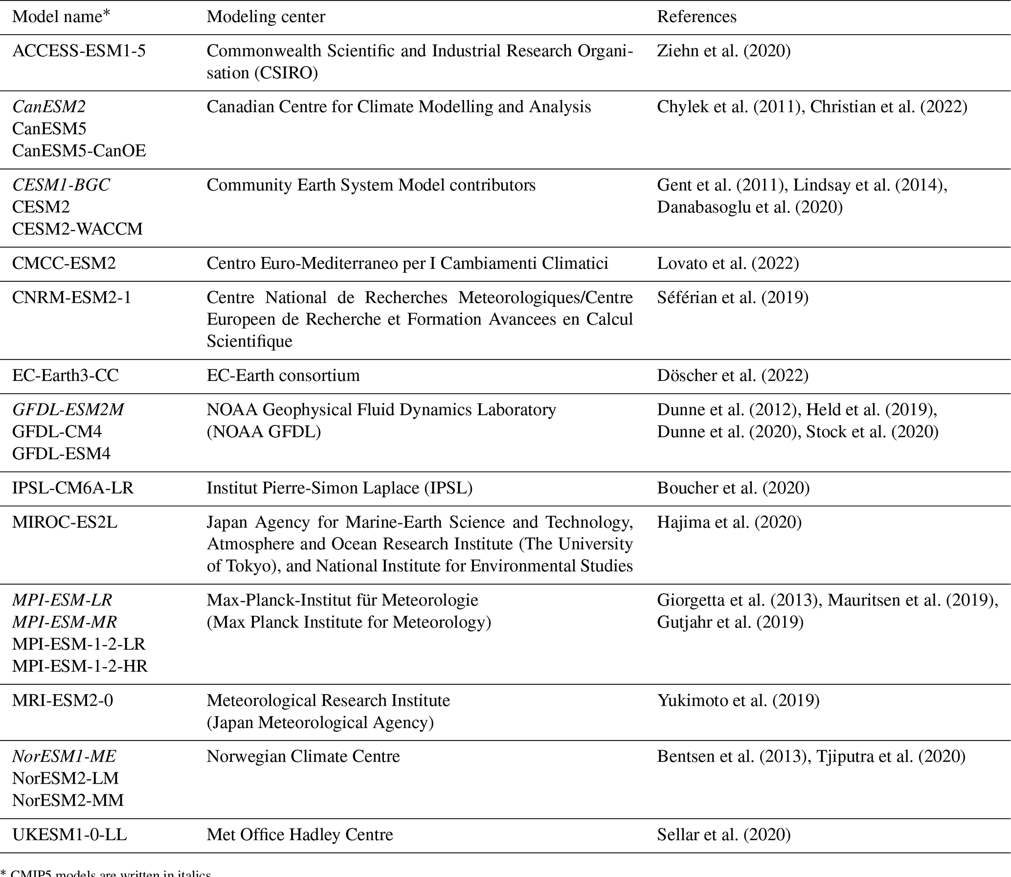
* CMIP5 models are written in italics.

Figure A1Correction of simulated anthropogenic carbon air–sea flux for the late starting date in Earth system models. (a) Multi-model annual mean anthropogenic carbon (Cant) air–sea flux for 17 ESMs from CMIP6 before (dashed lines) and after (solid lines) the correction for the late starting date over the historical period from 1850 to 2014 (black) and for the future from 2015 to 2100 under SSP1-2.6 (blue), SSP2-4.5 (orange), and SSP5-8.5 (red). (b) Cumulative ocean Cant uptake since 1765 (corrected simulated flux) and 1850 (raw simulated flux), (c) difference between cumulative ocean Cant uptake between corrected and raw simulated flux, and (d) the correction factor that was applied. The Cant correction that was estimated by Bronselaer et al. (2017) is shown in (c). The cumulative Cant uptake from 1765 to 1850 was set to 12 Pg C as estimated by Bronselaer et al. (2017).
Table A2Global ocean air–sea CO2 flux estimates based on 17 ESMs from CMIP6 before and after constraint over different periods with corrected and uncorrected estimates and with and without CNRM-ESM2-1. Prior uncertainty is the multi-model standard deviation, and constrained uncertainty is a combination of the multi-model standard deviation after correction and the uncertainty from the correction itself (see Sect. 3.1).

The analyzed variables include the air–sea CO2 flux (fgco2, name of the variable in standardized CMIP output), total dissolved inorganic carbon (dissic), total alkalinity (talk), total dissolved inorganic silicon (si), total dissolved inorganic phosphorus (po4), potential temperature (thetao), salinity (so), and the Atlantic meridional streamfunction (msftmz or msftyz). All ESMs were included for which the entire set of variables was available on the website of the Earth System Grid Federation at the start of the analysis. Based on these variables, all other presented variables were derived.
-
The air–sea Cant flux was calculated as the difference in air–sea CO2 flux between the historical plus future (SSP for CMIP6 and RCP (Representative Concentration Pathway) for CMIP5) simulation and the corresponding pre-industrial control simulation on the native model grids (where possible). The air–sea Cant fluxes were corrected for their late starting date in 1850 (and 1861 for GFDL-ESM2M) and the slightly higher atmospheric CO2 mixing ratio in that year compared to the beginning of industrialization and the start of the CO2 increase in 1765 (Bronselaer et al., 2017). To that end, we scaled the simulated air–sea Cant flux with the anthropogenic change in the atmospheric partial pressure of CO2 (pCO2) with respect to pre-industrial conditions following previous studies (Mikaloff Fletcher et al., 2006; Gruber et al., 2009; Terhaar et al., 2021b):
with Cant(t) being the simulated air–sea Cant flux by the respective ESM in year t and being the corrected air–sea Cant flux. For GFDL-ESM2M, which starts in 1861, the correction was made with respect to pCO2(1861). When pCO2(t) is close to pCO2(1850), their difference becomes unrealistically large, causing overly strong flux corrections. Therefore, we limited the flux correction in magnitude using the correction term in the year 1950 as an upper limit. By doing so, we do not only remove unrealistically high air–sea Cant fluxes before 1950 but also reach excellent agreement with the previously estimated air–sea Cant flux correction term of Bronselaer et al. (2017) (Fig. A1). When the cumulative Cant fluxes since 1765 are shown, an additional amount of 12 Pg C (16 Pg C for GFDL-ESM2M) was added that was estimated to have entered the ocean before 1850 (Bronselaer et al., 2017). For comparison, we also calculated the constrained estimates for the ocean Cant sink when no air–sea Cant flux correction is applied (Table A2). Bronselaer et al. (2017) estimate the uncertainty of the correction to be ± 16 % for cumulative Cant fluxes from 1765 to 1995. Although uncertainties reduce over time, we apply the 16 % from the past to all estimates and hence provide a conservative upper bound of this uncertainty.
-
Accordingly, the change in ocean interior Cant was calculated as the difference in total dissolved inorganic carbon between the historical plus future (SSP/RCP) simulation and the corresponding pre-industrial control simulation on the native model grids (where possible).
-
The change in air–sea CO2 flux that is caused by a changing climate was calculated as the difference in fgco2 in the historical simulation and the “bgc” simulation in which only atmospheric CO2 changes but not the climate. These “bgc” simulations were available for five ESMs (Table A3).
-
The surface ocean Revelle factor was calculated from sea surface total dissolved inorganic carbon (dissic), total alkalinity (talk), total dissolved inorganic silicon (si), total dissolved inorganic phosphorus (po4), potential temperature (thetao), and salinity (so) averaged around the year 2002 (from 1997 to 2007 for CMIP6 and 1999 to 2005 for CMIP5; 2005 is the last year of the historical simulation) using mocsy2.0 (Orr and Epitalon, 2015) with its default constants that are recommended for best practice (Dickson et al., 2007). The years were centered around 2002 to make the Revelle factor comparable to the one estimated based on GLODAPv2, which is normalized to the year 2002 (Lauvset et al., 2016). As the Revelle factor describes the relative change in CT per relative change in pCO2 (Revelle and Suess, 1957), the absolute uptake of CT does not only depend on the Revelle factor but also on the natural CT in the surface ocean. To calculate the buffer capacity for each ESM, the Revelle factor was therefore adjusted in each grid cell by multiplying it by the ratio of observed CT and the simulated CT in each ESM separately. Data from each ESM were regridded on a regular 1∘ × 1∘ grid to make them comparable to the gridded GLODAPv2 data. Furthermore, a mask was applied before the basin-wide-averaged Revelle factor was calculated so that only those values were used for which all ESMs and the gridded GLODAPv2 product had data. In addition, marginal seas (Mediterranean Sea, Hudson Bay, Baltic Sea) were excluded because global ESMs are not designed to accurately represent these small-scale seas. In addition, the surface ocean carbonate ion (CO) concentration was calculated so that the CT-adjusted Revelle factor is mainly determined by the CO concentrations, which itself can be approximated by the difference between surface ocean alkalinity and CT (Fig. A2).
-
The monthly AMOC strength was calculated as the maximum of the streamfunction below 500 m at the latitude in the respective model that is closest to 26.5∘ N for each month from 2004 to 2020. After 2014, simulated outputs from SSP5-8.5 and RCP4.5 were used as all ESMs provided output for these pathways. For SSP5-8.5, the mole fraction of atmospheric CO2 in SSP5-8.5 is 414.9 ppm in 2020 (Meinshausen et al., 2020), 2.5 ppm over the observed mole fraction of atmospheric CO2 in 2020 (NOAA/GML, 2022). For RCP4.5, the mole fraction of atmospheric CO2 is 412.4 ppm in 2020. Such small differences in the mole fraction of atmospheric CO2 do not cause detectable changes in global warming or the AMOC (IPCC, 2021).
-
Future saturation states of aragonite were calculated from simulated changes in total dissolved inorganic carbon (dissic), total alkalinity (talk), total dissolved inorganic silicon (si), total dissolved inorganic phosphorus (po4), potential temperature (thetao), and salinity (so) since 2002 that are added to the respective observed variables from the gridded GLODAPv2 product, which are normalized to 2002, using mocsy2.0 (Orr and Epitalon, 2015) with its default constants that are recommended for best practice (Dickson et al., 2007). By only adding simulated differences, model uncertainties in the initial state of the ocean biogeochemical system in the deeper ocean are removed (Orr et al., 2005; Terhaar et al., 2020a, 2021a, b). All variables were regridded before on a regular 1∘ × 1∘ grid so that they could be added to the gridded GLODAPv2 data. The same mask that was also used to compare the Revelle factor was applied to make all projections comparable.
-
The annual average sea surface salinity between the polar and subtropical front in the Southern Ocean was derived from regridded (1∘ × 1∘ regular grid) monthly sea surface salinity and temperatures (for defining the fronts) following Terhaar et al. (2021b).
-
The area of weakly stratified waters was calculated based on climatologies of the potential temperature and salinity from 1995 to 2014 (Hess, 2022). All data were regridded on a regular 1∘ × 1∘ grid with 33 depth levels before analysis. An area was defined as weakly stratified if the density gradient between the surface and the cell at 1000 m depth was smaller than 0.5 kg m−3 in a given month, assuming that such a small monthly mean gradient allows mixing of water into the lower limb of the AMOC at some time in that month. This predictor, as well as the different ways of calculating the Revelle factor predictor (see Sect. 5, “Robustness of the emergent constraint and possible impact of changing riverine carbon input over time”), was used to test the robustness of the emergent constraint identified here (Table A4).
The model CNRM-ESM2-1 was not used for the constraints because it includes dynamical riverine forcing that no other model includes (Fig. A4) and is not directly comparable. Instead, output from this ESM was prominently used in the section “Robustness of the emergent constraint and possible impact of changing riverine carbon input over time”. However, even if CNRM-ESM2-1 had been included, the results would change by less than 1 % (Table A2).
Table A3Climate-driven changes in the air–sea CO2 flux (Pg C yr−1) as simulated by five Earth system models from CMIP6.
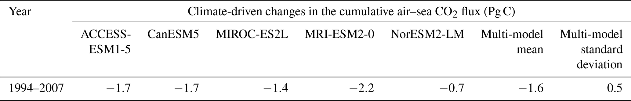
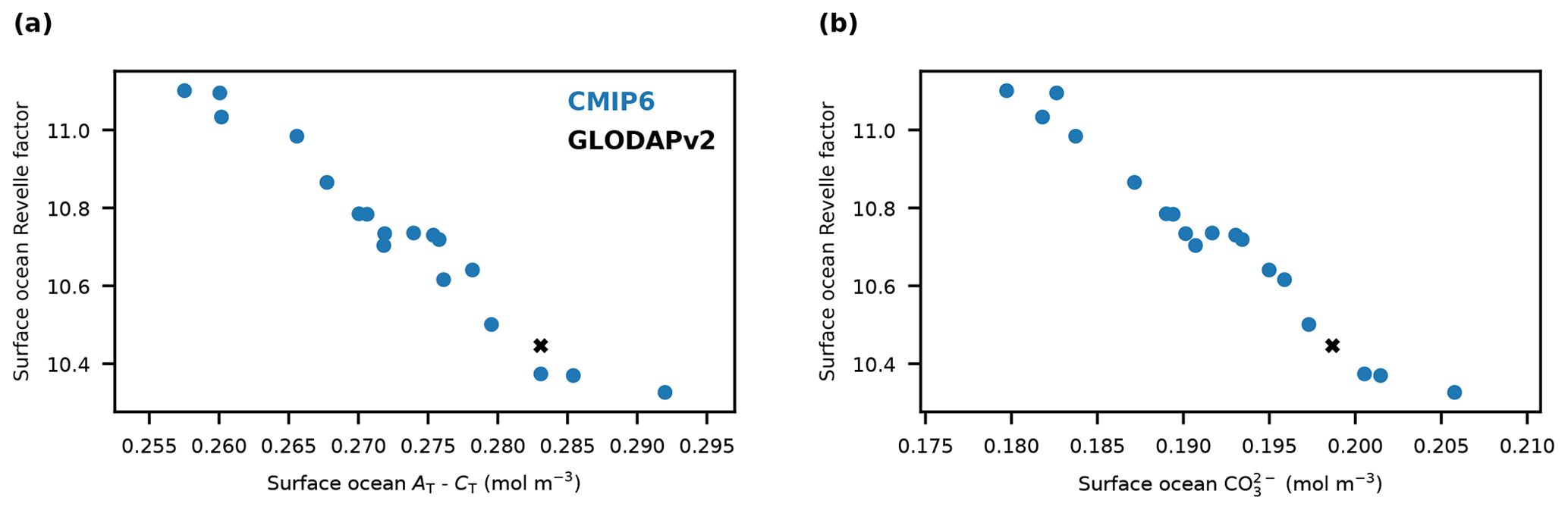
Figure A2Surface ocean Revelle factor against the difference of surface alkalinity and dissolved inorganic carbon, as well as against surface carbonate ion concentrations. Basin-wide-averaged surface ocean Revelle factor as simulated by 18 ESMs from CMIP6 (blue dots) against the basin-wide-averaged surface ocean (a) difference between total alkalinity (AT) and CT and (b) carbonate ion (CO) concentrations. The observation-based estimates from GLODAPv2 are shown as black crosses. The Revelle factor in each ESM was adjusted for biases in the surface ocean CT (see Sect. A1).
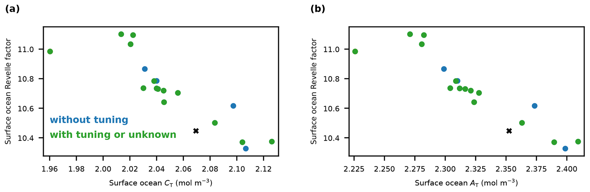
Figure A3Surface ocean Revelle factor against the surface alkalinity and dissolved inorganic carbon. Basin-wide-averaged surface ocean Revelle factor as simulated by 18 ESMs from CMIP6 (blue dots) against the basin-wide-averaged surface ocean (a) total alkalinity (AT) and (b) CT. The observation-based estimates from GLODAPv2 are shown as black crosses. The Revelle factor in each ESM was adjusted for biases in the surface ocean CT (see Sect. A1).
Table A4Constrained global ocean air–sea CO2 flux estimates based on 17 ESMs from CMIP6 with varying predictors.
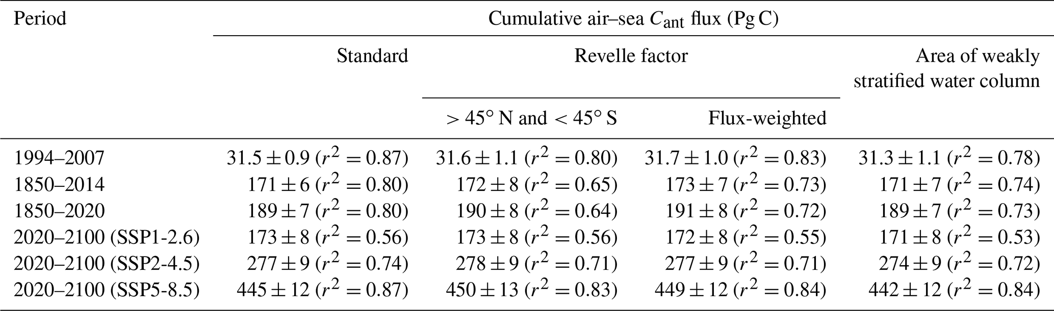

Figure A4Anthropogenic carbon air–sea fluxes and inventory changes simulated by CNRM-ESM2-1. (a) Cumulative air–sea anthropogenic carbon (Cant) fluxes (solid lines) and Cant interior changes (dashed lines) as simulated by CNRM-ESM2-1 for the historic period until 2014 (black) and from 2015 to 2100 under SSP1-2.6 (blue), SSP2-4.5 (orange), and SSP5-8.5 (red), (b) as well as the difference of both quantities. The thin dashed black line in (b) indicates zero difference.
A2 Observations and observation-based products
Throughout this paper, three observation-based products are used to constrain the ESM output.
Monthly climatologies of sea surface salinity and sea surface temperatures from the World Ocean Atlas 2018 (Zweng et al., 2018; Locarnini et al., 2018) were used to derive annual averages and uncertainties of the sea surface salinity between the polar and subtropical fronts in the Southern Ocean following Terhaar et al. (2021b). Climatologies of the World Ocean Atlas 2018 were also used to calculate the area of weakly stratified surface waters.
Time series of the AMOC strength from the RAPID array (McCarthy et al., 2020) were used to calculate monthly means and uncertainties of the AMOC from 2004 to 2020.
The gridded observation-based estimates of total dissolved inorganic carbon, total alkalinity, total dissolved inorganic silicon, total dissolved inorganic phosphorus, in situ temperature, and salinity from GLODAPv2 (Lauvset et al., 2016) were used to calculate the Revelle factor and acted as a starting point for projected saturation states over the 21st century (see above).
A3 Validation of the identified constraint in CMIP5
The emergent constraint identified here was derived from an ensemble of 17 ESMs from CMIP6. To test the robustness of emergent constraints, these constraints should be validated in an independent ensemble of ESMs (Hall et al., 2019). Here, we used all six ESMs from CMIP5, which provided all necessary output variables for this analysis (see Sect. A1). For all these models, the Cant uptake for the period from 1994 to 2007 and from 1850 to 2014 was predicted based on the simulated inter-frontal sea surface salinity in the Southern Ocean, the AMOC strength, and the global ocean basin-wide-averaged Revelle factor using the multi-linear relationship derived from the CMIP6 models (Fig. A5).
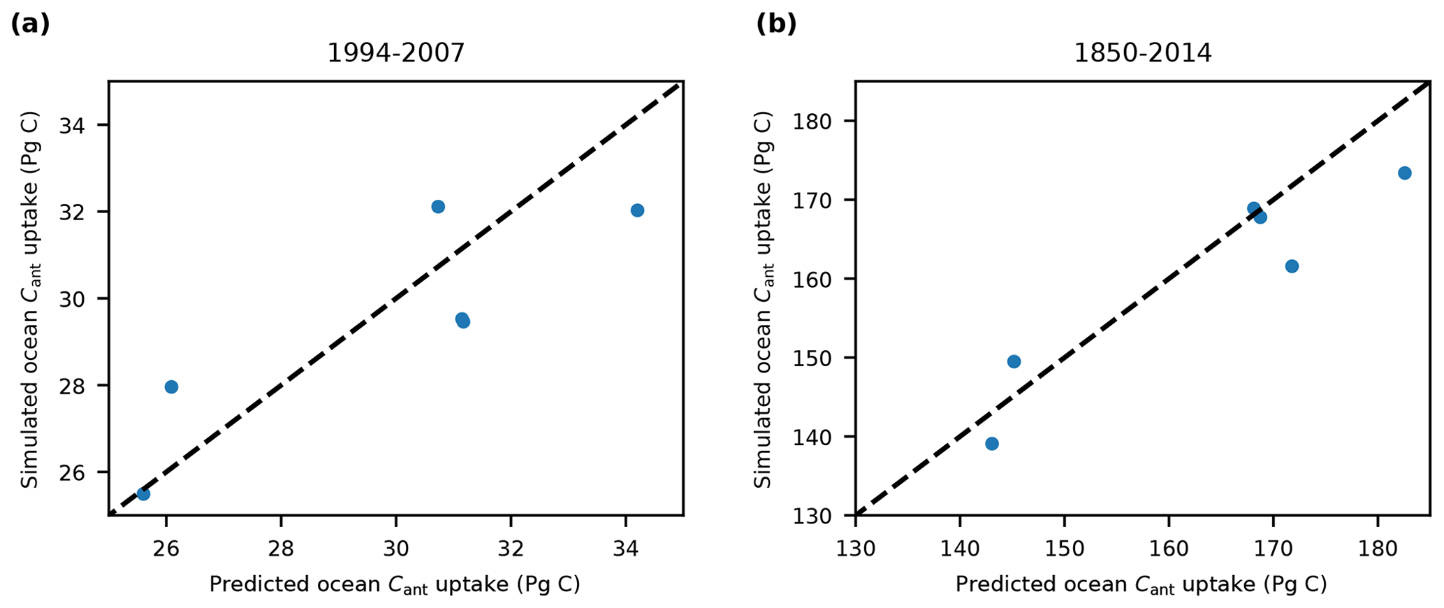
Figure A5Global ocean anthropogenic carbon uptake simulated by Earth system models from CMIP5 against the predicted uptake based on simulated predictors from CMIP6 models. Global ocean anthropogenic carbon uptake simulated by six ESMs from CMIP5 (Table A1) (a) from 1994 to 2007 and (b) from 1850 to 2014 against the predicted anthropogenic carbon uptake based on the simulated CMIP6 predictors in each ESM: the inter-frontal annual mean sea surface salinity in the Southern Ocean, the Atlantic Meridional Overturning Circulation, and the Revelle factor adjusted for surface ocean CT. Please note that two ESMs are at almost the same place in (a) with a predicted Cant uptake of around 31 Pg C.
A4 Comparison between simulated and observed CFC-11 concentrations
Comparison between simulated and observed CFC-11 uptake can be used to estimate the ventilation of waters from the surface waters to the deeper ocean (Hall et al., 2002). Although CFCs can roughly evaluate the ventilation rate of the ocean, no perfect agreement between CFCs and Cant can be expected as CFCs are not taken up at the same speed as Cant (i.e., fast air–sea equilibration timescale for CFC), and their solubility has a different temperature dependency than the solubility of Cant (warm waters can hold less CFCs but more Cant due to their low Revelle factor, whereas cold waters hold more CFCs but less Cant) (Revelle and Suess, 1957; Broecker and Peng, 1974; Weiss, 1974). These differences can lead to differences between uptake, storage, and distribution of CFCs and Cant that can become especially large in high-latitude oceans (Matear et al., 2003; Terhaar et al., 2020b).
Here, we use simulated CFC-11 from ESMs and observed CFC-11 from GLODAPv2.2021 (Lauvset et al., 2021) to provide further evidence that the inter-frontal sea surface salinity in the Southern Ocean and the AMOC are good indicators of the ocean ventilation and that ESMs tend to underestimate the ventilation of surface waters to the deeper ocean. Out of the 18 ESMs from CMIP6, 10 provided simulated three-dimensional fields of CFC-11 (CanESM5, CESM2, CESM2-WACCM, EC-Earth-CC, GFDL-CM4, GFDL-ESM4, MRI-ESM2-0, NorESM2-LM, NorESM2-MM, UKESM1-0-LL). To compare these ESMs to the observed concentrations, all ESMs were sampled at the same time (month and year), the same latitude and longitude, and the same depth as the observations. To assess the ventilation below the mixed layer, we only used observations below 200 m. Furthermore, we limited our assessment to observations until 2004 as CFC-11 in the atmosphere peaked in 1994 (Bullister, 2017), and subducted waters since then might already re-emerge to the surface. Thus, 506 000 measurements remained. As these measurements are not equally distributed and strongly clustered in the Northern Hemisphere (Lauvset et al., 2021), we mapped all measurements on a regular 5∘ × 5∘ grid with 11 depth levels from 200 to 6000 m that increase with depth. In each cell on the grid the average bias was calculated. Afterwards, the volume-averaged bias was calculated for the Southern Hemisphere and the North Atlantic (limited by the Equator and 65∘ N) (Fig. A6).
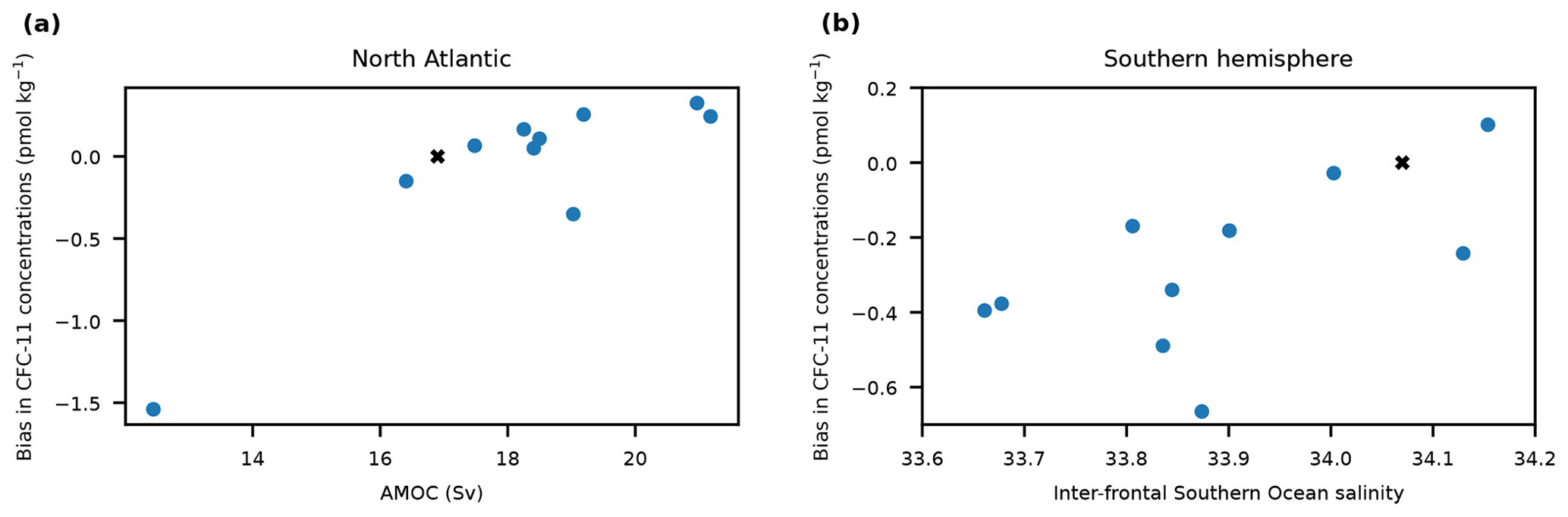
Figure A6Biases in subsurface CFC-11 concentrations between observations against the Atlantic Meridional Overturning Circulation and the inter-frontal Southern Ocean salinity. Basin-wide-averaged biases in CFC-11 concentrations (observations minus simulated) below 200 m for all 10 ESMs that provided simulated CFC-11 (blue dots) (a) in the North Atlantic Ocean (north of the Equator and limited by the Fram Strait, the Barents Sea Opening, and Baffin Bay) and against the AMOC and (b) in the Southern Hemisphere (south of the Equator) against the inter-frontal annual mean sea surface salinity in the Southern Ocean. The observation-based estimates for the AMOC and the inter-frontal annual mean sea surface salinity in the Southern Ocean are shown as black crosses and with zero bias in CFC-11.
A5 Comparison between simulated and observation-based estimates of the interior ocean Cant accumulation
Another way to test the emergent constraint identified here is the comparison to observation-based estimates of the interior ocean Cant accumulation. Here, we compare model results against the estimate for interior ocean Cant accumulation from 1800 to 1994 (Sabine et al., 2004) and from 1994 to 2007 (Gruber et al., 2019a), although different reconstruction methods yield different results (e.g., Khatiwala et al., 2013, their Fig. 4). While a good representation of the interior ocean Cant distribution is not necessarily related to a correct estimate of the air–sea Cant flux, it can provide an indication of the model performance and the robustness of the applied corrections. For both comparisons, we compare the multi-model mean and standard deviation and results from the ESM that represent best the three observational predictors (i.e., GFDL-ESM4). GFDL-ESM4 has a global ocean Revelle factor of 10.37, an inter-frontal sea surface salinity of 34.00, and an AMOC of 18.25. The biases that may exist in the multi-model mean, such as relatively little Cant in the Southern Hemisphere due to a multi-model-averaged sea surface salinity that is too low compared to observed sea surface salinities, should be smaller for GFDL-ESM4.
The comparison to the observation-based estimate of Cant accumulation from 1800 to 1994 (Sabine et al., 2004) demonstrates that the ESMs represent the distribution of Cant in the ocean between the basins and different latitudinal regions well (Table A5). Small underestimations exist in the Indian and Atlantic tropical oceans, as well as in the southern subpolar Atlantic Ocean. The differences in the Indian Ocean may well be to observational uncertainties that are especially large in this relatively under-sampled ocean basin (Sabine et al., 2004; Gruber et al., 2019a). The underestimation in the Southern Atlantic and the Atlantic sector of the Southern Ocean are consistent with an underestimation of the formation of mode and intermediate waters in the Southern Ocean due to a sea surface salinity that is too low. This underestimation is strongly reduced in the GFDL-ESM4 model (Table A6), indicating that the better representation of the inter-frontal sea surface salinity in the Southern Ocean also improves the simulated distribution of Cant in the ocean. Furthermore, GFDL-ESM4 also simulates slightly higher Cant in the North Atlantic, consistent with its AMOC being slightly too high.
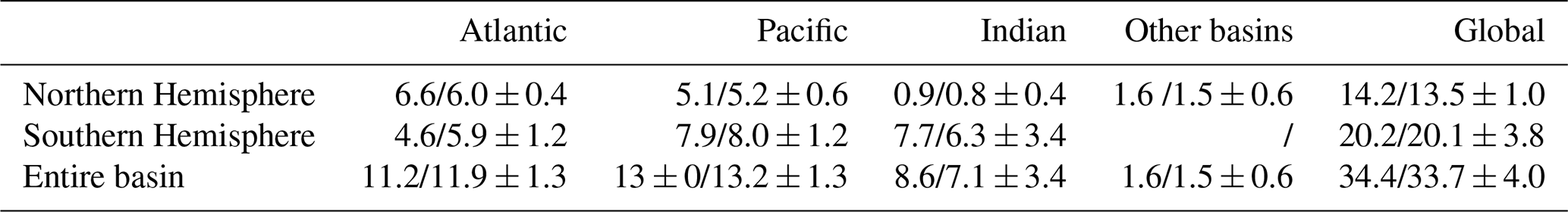
The comparison for the period from 1994 to 2007 also indicates that the ESMs on average simulate the Cant interior storage pattern as estimated based on observations of Gruber et al. (2019a) (Table A7). The ESMs agree with the observation-based estimates with respect to the basin and hemispheric distribution. However, they underestimate on average the storage in the Southern Hemisphere in line with the underestimation of the formation of intermediate and mode waters in the Southern Ocean. When only considering GFDL-ESM4 (Table A8), this underestimation is reduced, and all other regions show very good agreement.
The remaining small difference in both comparisons may be also due to different alignments of the basin boundaries, an unknown distribution of the Cant that entered the ocean before 1850 and has been advected 50 years longer in the ocean interior in the case of Sabine et al. (2004), a different decadal variability in GFDL-ESM4 than in the real world in the case of Gruber et al. (2019a), and uncertainties in the observation-based estimates. Despite all these potential pitfalls, the three-dimensional repartition of Cant between observation-based products and ESMs agree, and the model that best simulates the three key predictors, GFDL-ESM4, is almost identical to the observation-based estimates.
Table A5Distribution of Cant inventories (in Pg C) by basin and latitude band for 1994. The first number in each cell is the multi-model mean and standard deviation across all 18 ESMs from CMIP6, and the second number is from Table S1 in Sabine et al. (2004).
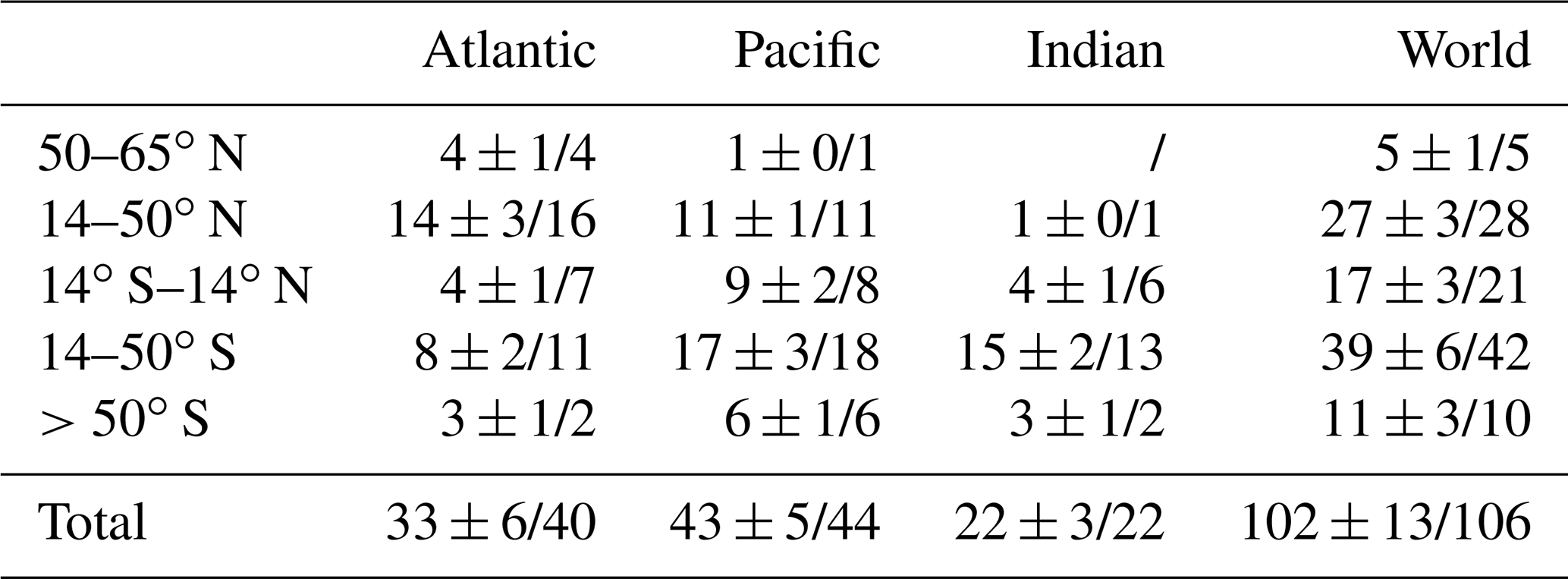
Table A6Distribution of Cant inventories (in Pg C) by basin and latitude band for 1994. The first number in each cell is derived from GFDL-ESM4, and the second number is from Table S1 in Sabine et al. (2004).
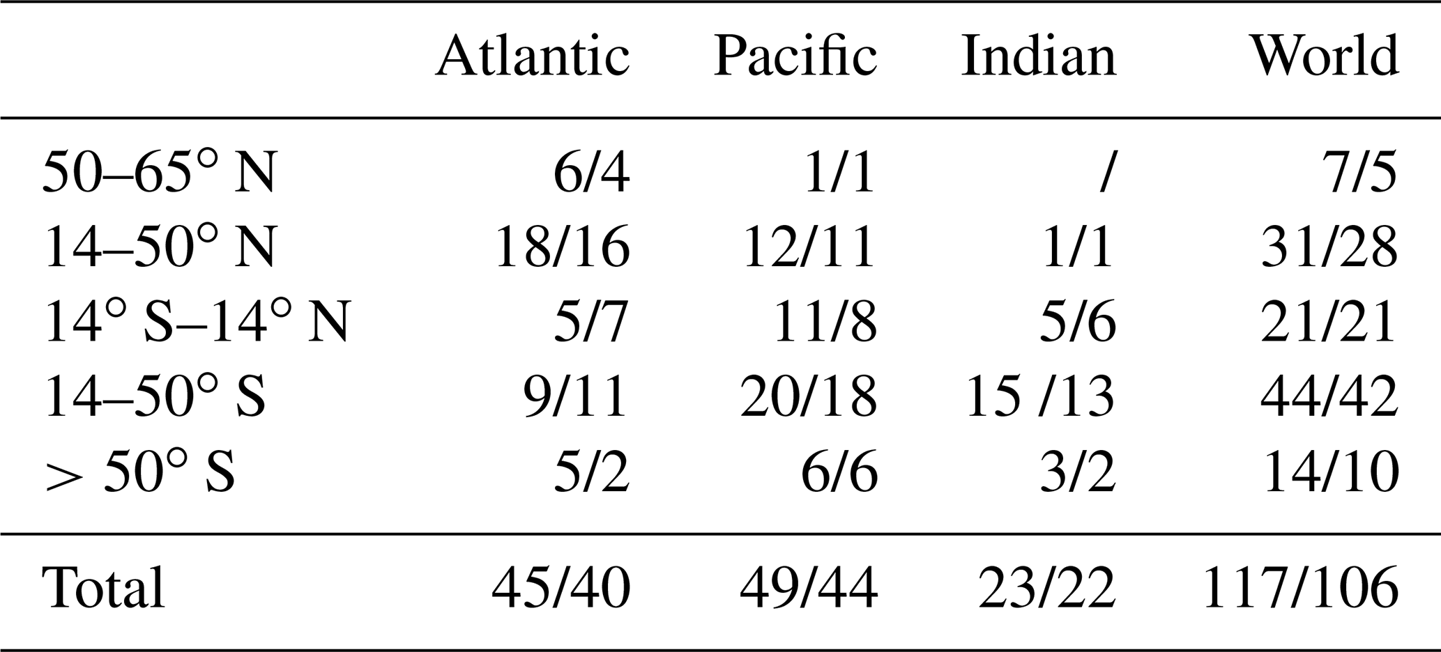
Table A7Distribution of Cant inventories (in Pg C) by basin and hemisphere from 1994 to 2007. The first number in each cell is the multi-model mean and standard deviation across all 18 ESMs from CMIP6, and the second number is from Table 1 in Gruber et al. (2019a).
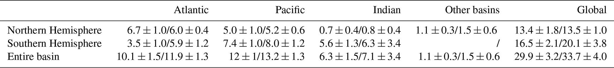
Table A8Distribution of Cant inventories (in Pg C) by basin and hemisphere from 1994 to 2007. The first number in each cell is derived from GFDL-ESM4, and the second number is from Table 1 in Gruber et al. (2019a).
The mocsy2.0 code is publicly available via https://github.com/jamesorr/mocsy (Orr and Epitalon, 2015).
The Earth system model output used in this study is available via the Earth System Grid Federation (https://esgf-node.ipsl.upmc.fr/projects/esgf-ipsl/, last access: 1 June 2022). For further information, please see Table A1.
JT was responsible for conceptualization, methodology, software, investigation, visualization, and writing the original draft. TLF and FJ were responsible for funding acquisition. TLF and FJ were responsible for project administration. JT, TLF, and FJ were responsible for writing, review, and editing.
The contact author has declared that none of the authors has any competing interests.
The work reflects only the authors' view; the European
Commission and their executive agency are not responsible for any use that
may be made of the information the work contains.
Publisher's note: Copernicus Publications remains neutral with regard to jurisdictional claims in published maps and institutional affiliations.
This work was funded by the European Union's Horizon 2020 research and innovation program under grant agreement no. 821003 (project 4C, Climate–Carbon Interactions in the Current Century) (Jens Terhaar, Thomas L. Frölicher, Fortunat Joos) and no. 820989 (project COMFORT, Our common future ocean in the Earth system-quantifying coupled cycles of carbon, oxygen and nutrients for determining and achieving safe operating spaces with respect to tipping points) (Thomas L. Frölicher, Fortunat Joos), as well as by the Swiss National Science Foundation under grant PP00P2_198897 (Thomas L. Frölicher) and grant #200020_200511 (Jens Terhaar, Fortunat Joos). We also thank Donat Hess for his work on the North Atlantic anthropogenic carbon uptake during his master thesis at our institute, as well as Friedrich Burger, Nadine Goris, and Jens Müller for discussions. We also thank one anonymous reviewer and Roland Séférian for their careful and helpful assessment of our manuscript and Jack Middelburg for his efficient editorial handling.
This research has been supported by the Horizon 2020 (4C (grant no. 821003) and COMFORT (grant no. 820989)) and the Schweizerischer Nationalfonds zur Förderung der Wissenschaftlichen Forschung (grant nos. 200020_200511 and PP00P2_198897).
This paper was edited by Jack Middelburg and reviewed by Roland Séférian and one anonymous referee.
Albright, R., Caldeira, L., Hosfelt, J., Kwiatkowski, L., Maclaren, J. K., Mason, B. M., Nebuchina, Y., Ninokawa, A., Pongratz, J., Ricke, K. L., Rivlin, T., Schneider, K., Sesboüé, M., Shamberger, K., Silverman, J., Wolfe, K., Zhu, K., and Caldeira, K.: Reversal of ocean acidification enhances net coral reef calcification, Nature, 531, 362–365, https://doi.org/10.1038/nature17155, 2016.
Aumont, O., Orr, J. C., Monfray, P., Ludwig, W., Amiotte-Suchet, P., and Probst, J.-L.: Riverine-driven interhemispheric transport of carbon, Global Biogeochem. Cy., 15, 393–405, https://doi.org/10.1029/1999GB001238, 2001.
Bakker, P., Schmittner, A., Lenaerts, J. T. M., Abe-Ouchi, A., Bi, D., van den Broeke, M. R., Chan, W.-L., Hu, A., Beadling, R. L., Marsland, S. J., Mernild, S. H., Saenko, O. A., Swingedouw, D., Sullivan, A., and Yin, J.: Fate of the Atlantic Meridional Overturning Circulation: Strong decline under continued warming and Greenland melting, Geophys. Res. Lett., 43, 12252–12260, https://doi.org/10.1002/2016GL070457, 2016.
Bednaršek, N., Tarling, G. A., Bakker, D. C. E., Fielding, S., and Feely, R. A.: Dissolution Dominating Calcification Process in Polar Pteropods Close to the Point of Aragonite Undersaturation, PLoS One, 9, e109183, https://doi.org/10.1371/journal.pone.0109183, 2014.
Behrenfeld, M. J., Gaube, P., Della Penna, A., O'Malley, R. T., Burt, W. J., Hu, Y., Bontempi, P. S., Steinberg, D. K., Boss, E. S., Siegel, D. A., Hostetler, C. A., Tortell, P. D., and Doney, S. C.: Global satellite-observed daily vertical migrations of ocean animals, Nature, 576, 257–261, https://doi.org/10.1038/s41586-019-1796-9, 2019.
Bennington, V., Gloege, L., and McKinley, G. A.: Variability in the global ocean carbon sink from 1959 to 2020 by correcting models with observations, Geophys. Res. Lett., 49, e2022GL098632, https://doi.org/10.1029/2022GL098632, 2022.
Bentsen, M., Bethke, I., Debernard, J. B., Iversen, T., Kirkevåg, A., Seland, Ø., Drange, H., Roelandt, C., Seierstad, I. A., Hoose, C., and Kristjánsson, J. E.: The Norwegian Earth System Model, NorESM1-M – Part 1: Description and basic evaluation of the physical climate, Geosci. Model Dev., 6, 687–720, https://doi.org/10.5194/gmd-6-687-2013, 2013.
Boucher, O., Servonnat, J., Albright, A. L., Aumont, O., Balkanski, Y., Bastrikov, V., Bekki, S., Bonnet, R., Bony, S., Bopp, L., Braconnot, P., Brockmann, P., Cadule, P., Caubel, A., Cheruy, F., Codron, F., Cozic, A., Cugnet, D., D'Andrea, F., Davini, P., de Lavergne, C., Denvil, S., Deshayes, J., Devilliers, M., Ducharne, A., Dufresne, J.-L., Dupont, E., Éthé, C., Fairhead, L., Falletti, L., Flavoni, S., Foujols, M.-A., Gardoll, S., Gastineau, G., Ghattas, J., Grandpeix, J.-Y., Guenet, B., Guez E., L., Guilyardi, E., Guimberteau, M., Hauglustaine, D., Hourdin, F., Idelkadi, A., Joussaume, S., Kageyama, M., Khodri, M., Krinner, G., Lebas, N., Levavasseur, G., Lévy, C., Li, L., Lott, F., Lurton, T., Luyssaert, S., Madec, G., Madeleine, J.-B., Maignan, F., Marchand, M., Marti, O., Mellul, L., Meurdesoif, Y., Mignot, J., Musat, I., Ottlé, C., Peylin, P., Planton, Y., Polcher, J., Rio, C., Rochetin, N., Rousset, C., Sepulchre, P., Sima, A., Swingedouw, D., Thiéblemont, R., Traore, A. K., Vancoppenolle, M., Vial, J., Vialard, J., Viovy, N., and Vuichard, N.: Presentation and Evaluation of the IPSL-CM6A-LR Climate Model, J. Adv. Model. Earth Sy., 12, e2019MS002010, https://doi.org/10.1029/2019MS002010, 2020.
Bourgeois, T., Goris, N., Schwinger, J., and Tjiputra, J. F.: Stratification constrains future heat and carbon uptake in the Southern Ocean between 30∘ S and 55∘ S, Nat. Commun., 13, 340, https://doi.org/10.1038/s41467-022-27979-5, 2022.
Brient, F.: Reducing Uncertainties in Climate Projections with Emergent Constraints: Concepts, Examples and Prospects, Adv. Atmos. Sci., 37, 1–15, https://doi.org/10.1007/s00376-019-9140-8, 2020.
Broecker, W. S. and Peng, T.-H.: Gas exchange rates between air and sea, Tellus, 26, 21–35, https://doi.org/10.1111/j.2153-3490.1974.tb01948.x, 1974.
Bronselaer, B., Winton, M., Russell, J., Sabine, C. L., and Khatiwala, S.: Agreement of CMIP5 Simulated and Observed Ocean Anthropogenic CO2 Uptake, Geophys. Res. Lett., 44, 212–298, https://doi.org/10.1002/2017GL074435, 2017.
Brown, P. J., McDonagh, E. L., Sanders, R., Watson, A. J., Wanninkhof, R., King, B. A., Smeed, D. A., Baringer, M. O., Meinen, C. S., Schuster, U., Yool, A., and Messias, M.-J.: Circulation-driven variability of Atlantic anthropogenic carbon transports and uptake, Nat. Geosci., 14, 571–577, https://doi.org/10.1038/s41561-021-00774-5, 2021.
Buckley, M. W. and Marshall, J.: Observations, inferences, and mechanisms of the Atlantic Meridional Overturning Circulation: A review, Rev. Geophys., 54, 5–63, https://doi.org/10.1002/2015RG000493, 2016.
Bullister, J. L.: Atmospheric Histories (1765–2015) for CFC-11, CFC-12, CFC-113, CCl4, SF6 and N2O (NCEI Accession 0164584), NOAA National Centers for Environmental Information [data set], https://doi.org/10.3334/CDIAC/otg.CFC_ATM_Hist_2015, 2017.
Bushinsky, S. M., Landschützer, P., Rödenbeck, C., Gray, A. R., Baker, D., Mazloff, M. R., Resplandy, L., Johnson, K. S., and Sarmiento, J. L.: Reassessing Southern Ocean Air-Sea CO2 Flux Estimates With the Addition of Biogeochemical Float Observations, Global Biogeochem. Cy., 33, 1370–1388, https://doi.org/10.1029/2019GB006176, 2019.
Caldeira, K. and Duffy, P. B.: The Role of the Southern Ocean in Uptake and Storage of Anthropogenic Carbon Dioxide, Science, 287, 620–622, https://doi.org/10.1126/science.287.5453.620, 2000.
Caldwell, P. M., Bretherton, C. S., Zelinka, M. D., Klein, S. A., Santer, B. D., and Sanderson, B. M.: Statistical significance of climate sensitivity predictors obtained by data mining, Geophys. Res. Lett., 41, 1803–1808, https://doi.org/10.1002/2014GL059205, 2014.
Canadell, J. G., Monteiro, P. M. S., Costa, M. H., Cotrim da Cunha, L., Cox, P. M., Eliseev, A. V., Henson, S., Ishii, M., Jaccard, S., Koven, C., Lohila, A., Patra, P. K., Piao, S., Rogelj, J., Syampungani, S., Zaehle, S., and Zickfeld, K.: Global Carbon and other Biogeochemical Cycles and Feedbacks. In Climate Change 2021: The Physical Science Basis. Contribution of Working Group I to the Sixth Assessment Report of the Intergovernmental Panel on Climate Change, edited by: Masson-Delmotte, V., Zhai, P., Pirani, A., Connors, S. L., Péan, C., Berger, S., Caud, N., Chen, Y., Goldfarb, L., Gomis, M. I., Huang, M., Leitzell, K., Lonnoy,E., Matthews, J. B. R., Maycock, T. K., Waterfield, T., Yelekçi, O., Yu, R., and Zhou, B., Cambridge University Press, Cambridge, United Kingdom and New York, NY, USA, 673–816, https://doi.org/10.1017/9781009157896.007, 2021.
Chau, T. T. T., Gehlen, M., and Chevallier, F.: A seamless ensemble-based reconstruction of surface ocean pCO2 and air–sea CO2 fluxes over the global coastal and open oceans, Biogeosciences, 19, 1087–1109, https://doi.org/10.5194/bg-19-1087-2022, 2022.
Christian, J. R., Denman, K. L., Hayashida, H., Holdsworth, A. M., Lee, W. G., Riche, O. G. J., Shao, A. E., Steiner, N., and Swart, N. C.: Ocean biogeochemistry in the Canadian Earth System Model version 5.0.3: CanESM5 and CanESM5-CanOE, Geosci. Model Dev., 15, 4393–4424, https://doi.org/10.5194/gmd-15-4393-2022, 2022.
Chylek, P., Li, J., Dubey, M. K., Wang, M., and Lesins, G.: Observed and model simulated 20th century Arctic temperature variability: Canadian Earth System Model CanESM2, Atmos. Chem. Phys. Discuss., 11, 22893–22907, https://doi.org/10.5194/acpd-11-22893-2011, 2011.
Claustre, H., Johnson, K. S., and Takeshita, Y.: Observing the Global Ocean with Biogeochemical-Argo, Annu. Rev. Mar. Sci., 12, 23–48, https://doi.org/10.1146/annurev-marine-010419-010956, 2020.
Clement, D. and Gruber, N.: The eMLR(C*) Method to Determine Decadal Changes in the Global Ocean Storage of Anthropogenic CO2, Global Biogeochem. Cy., 32, 654–679, https://doi.org/10.1002/2017GB005819, 2018.
Danabasoglu, G., Lamarque, J.-F., Bacmeister, J., Bailey, D. A., DuVivier, A. K., Edwards, J., Emmons, L. K., Fasullo, J., Garcia, R., Gettelman, A., Hannay, C., Holland, M. M., Large, W. G., Lauritzen, P. H., Lawrence, D. M., Lenaerts, J. T. M., Lindsay, K., Lipscomb, W. H., Mills, M. J., Neale, R., Oleson, K. W., Otto-Bliesner, B., Phillips, A. S., Sacks, W., Tilmes, S., van Kampenhout, L., Vertenstein, M., Bertini, A., Dennis, J., Deser, C., Fischer, C., Fox-Kemper, B., Kay, J. E., Kinnison, D., Kushner, P. J., Larson, V. E., Long, M. C., Mickelson, S., Moore, J. K., Nienhouse, E., Polvani, L., Rasch, P. J., and Strand, W. G.: The Community Earth System Model Version 2 (CESM2), J. Adv. Model. Earth Sy., 12, e2019MS001916, https://doi.org/10.1029/2019MS001916, 2020.
DeVries, T.: The oceanic anthropogenic CO2 sink: Storage, air-sea fluxes, and transports over the industrial era, Global Biogeochem. Cy., 28, 631–647, https://doi.org/10.1002/2013GB004739, 2014.
Dickson, A. G., Sabine, C. L., and Christian, J. R. (Eds.): Guide to Best Practices for Ocean CO2 Measurements, PICES Special Publication 3, 191 pp., North Pacific Marine Science Organization Sidney, British Columbia, https://doi.org/10.25607/OBP-1342, 2007.
Doney, S. C., Busch, D. S., Cooley, S. R., and Kroeker, K. J.: The Impacts of Ocean Acidification on Marine Ecosystems and Reliant Human Communities, Annu. Rev. Env. Resour., 45, 83–112, https://doi.org/10.1146/annurev-environ-012320-083019, 2020.
Döscher, R., Acosta, M., Alessandri, A., Anthoni, P., Arsouze, T., Bergman, T., Bernardello, R., Boussetta, S., Caron, L.-P., Carver, G., Castrillo, M., Catalano, F., Cvijanovic, I., Davini, P., Dekker, E., Doblas-Reyes, F. J., Docquier, D., Echevarria, P., Fladrich, U., Fuentes-Franco, R., Gröger, M., v. Hardenberg, J., Hieronymus, J., Karami, M. P., Keskinen, J.-P., Koenigk, T., Makkonen, R., Massonnet, F., Ménégoz, M., Miller, P. A., Moreno-Chamarro, E., Nieradzik, L., van Noije, T., Nolan, P., O'Donnell, D., Ollinaho, P., van den Oord, G., Ortega, P., Prims, O. T., Ramos, A., Reerink, T., Rousset, C., Ruprich-Robert, Y., Le Sager, P., Schmith, T., Schrödner, R., Serva, F., Sicardi, V., Sloth Madsen, M., Smith, B., Tian, T., Tourigny, E., Uotila, P., Vancoppenolle, M., Wang, S., Wårlind, D., Willén, U., Wyser, K., Yang, S., Yepes-Arbós, X., and Zhang, Q.: The EC-Earth3 Earth system model for the Coupled Model Intercomparison Project 6, Geosci. Model Dev., 15, 2973–3020, https://doi.org/10.5194/gmd-15-2973-2022, 2022.
Dufour, C. O., Griffies, S. M., de Souza, G. F., Frenger, I., Morrison, A. K., Palter, J. B., Sarmiento, J. L., Galbraith, E. D., Dunne, J. P., Anderson, W. G., and Slater, R. D.: Role of Mesoscale Eddies in Cross-Frontal Transport of Heat and Biogeochemical Tracers in the Southern Ocean, J. Phys. Oceanogr., 45, 3057–3081, https://doi.org/10.1175/JPO-D-14-0240.1, 2015.
Dunne, J. P., John, J. G., Adcroft, A. J., Griffies, S. M., Hallberg, R. W., Shevliakova, E., Stouffer, R. J., Cooke, W., Dunne, K. A., Harrison, M. J., Krasting, J. P., Malyshev, S. L., Milly, P. C. D., Phillipps, P. J., Sentman, L. T., Samuels, B. L., Spelman, M. J., Winton, M., Wittenberg, A. T., and Zadeh, N.: GFDL's ESM2 Global Coupled Climate–Carbon Earth System Models. Part I: Physical Formulation and Baseline Simulation Characteristics, J. Climate, 25, 6646–6665, https://doi.org/10.1175/JCLI-D-11-00560.1, 2012.
Dunne, J. P., Horowitz, L. W., Adcroft, A. J., Ginoux, P., Held, I. M., John, J. G., Krasting, J. P., Malyshev, S., Naik, V., Paulot, F., Shevliakova, E., Stock, C. A., Zadeh, N., Balaji, V., Blanton, C., Dunne, K. A., Dupuis, C., Durachta, J., Dussin, R., Gauthier, P. P. G., Griffies, S. M., Guo, H., Hallberg, R. W., Harrison, M., He, J., Hurlin, W., McHugh, C., Menzel, R., Milly, P. C. D., Nikonov, S., Paynter, D. J., Ploshay, J., Radhakrishnan, A., Rand, K., Reichl, B. G., Robinson, T., Schwarzkopf, D. M., Sentman, L. T., Underwood, S., Vahlenkamp, H., Winton, M., Wittenberg, A. T., Wyman, B., Zeng, Y., and Zhao, M.: The GFDL Earth System Model Version 4.1 (GFDL-ESM 4.1): Overall Coupled Model Description and Simulation Characteristics, J. Adv. Model. Earth Sy., 12, e2019MS002015, https://doi.org/10.1029/2019MS002015, 2020.
Egleston, E. S., Sabine, C. L., and Morel, F. M. M.: Revelle revisited: Buffer factors that quantify the response of ocean chemistry to changes in DIC and alkalinity, Global Biogeochem. Cy., 24, GB1002, https://doi.org/10.1029/2008GB003407, 2010.
Eyring, V., Cox, P. M., Flato, G. M., Gleckler, P. J., Abramowitz, G., Caldwell, P., Collins, W. D., Gier, B. K., Hall, A. D., Hoffman, F. M., Hurtt, G. C., Jahn, A., Jones, C. D., Klein, S. A., Krasting, J. P., Kwiatkowski, L., Lorenz, R., Maloney, E., Meehl, G. A., Pendergrass, A. G., Pincus, R., Ruane, A. C., Russell, J. L., Sanderson, B. M., Santer, B. D., Sherwood, S. C., Simpson, I. R., Stouffer, R. J., and Williamson, M. S.: Taking climate model evaluation to the next level, Nat. Clim. Change, 9, 102–110, https://doi.org/10.1038/s41558-018-0355-y, 2019.
Fabry, V. J., Seibel, B. A., Feely, R. A., and Orr, J. C.: Impacts of ocean acidification on marine fauna and ecosystem processes, ICES J. Mar. Sci., 65, 414–432, https://doi.org/10.1093/icesjms/fsn048, 2008.
Falkowski, P. G., Barber, R. T., and Smetacek, V.: Biogeochemical Controls and Feedbacks on Ocean Primary Production, Science, 281, 200–206, https://doi.org/10.1126/science.281.5374.200, 1998.
Friedlingstein, P., Jones, M. W., O'Sullivan, M., Andrew, R. M., Bakker, D. C. E., Hauck, J., Le Quéré, C., Peters, G. P., Peters, W., Pongratz, J., Sitch, S., Canadell, J. G., Ciais, P., Jackson, R. B., Alin, S. R., Anthoni, P., Bates, N. R., Becker, M., Bellouin, N., Bopp, L., Chau, T. T. T., Chevallier, F., Chini, L. P., Cronin, M., Currie, K. I., Decharme, B., Djeutchouang, L. M., Dou, X., Evans, W., Feely, R. A., Feng, L., Gasser, T., Gilfillan, D., Gkritzalis, T., Grassi, G., Gregor, L., Gruber, N., Gürses, Ö., Harris, I., Houghton, R. A., Hurtt, G. C., Iida, Y., Ilyina, T., Luijkx, I. T., Jain, A., Jones, S. D., Kato, E., Kennedy, D., Klein Goldewijk, K., Knauer, J., Korsbakken, J. I., Körtzinger, A., Landschützer, P., Lauvset, S. K., Lefèvre, N., Lienert, S., Liu, J., Marland, G., McGuire, P. C., Melton, J. R., Munro, D. R., Nabel, J. E. M. S., Nakaoka, S.-I., Niwa, Y., Ono, T., Pierrot, D., Poulter, B., Rehder, G., Resplandy, L., Robertson, E., Rödenbeck, C., Rosan, T. M., Schwinger, J., Schwingshackl, C., Séférian, R., Sutton, A. J., Sweeney, C., Tanhua, T., Tans, P. P., Tian, H., Tilbrook, B., Tubiello, F., van der Werf, G. R., Vuichard, N., Wada, C., Wanninkhof, R., Watson, A. J., Willis, D., Wiltshire, A. J., Yuan, W., Yue, C., Yue, X., Zaehle, S., and Zeng, J.: Global Carbon Budget 2021, Earth Syst. Sci. Data, 14, 1917–2005, https://doi.org/10.5194/essd-14-1917-2022, 2022.
Frölicher, T. L. and Joos, F.: Reversible and irreversible impacts of greenhouse gas emissions in multi-century projections with the NCAR global coupled carbon cycle-climate model, Clim. Dynam., 35, 1439–1459, https://doi.org/10.1007/s00382-009-0727-0, 2010.
Frölicher, T. L., Sarmiento, J. L., Paynter, D. J., Dunne, J. P., Krasting, J. P., and Winton, M.: Dominance of the Southern Ocean in Anthropogenic Carbon and Heat Uptake in CMIP5 Models, J. Climate, 28, 862–886, https://doi.org/10.1175/JCLI-D-14-00117.1, 2015.
Gattuso, J.-P. and Hansson, L. (Eds.): Ocean acidification, Oxford University Press, ISBN 9780199591091, 2011.
Gent, P. R., Danabasoglu, G., Donner, L. J., Holland, M. M., Hunke, E. C., Jayne, S. R., Lawrence, D. M., Neale, R. B., Rasch, P. J., Vertenstein, M., Worley, P. H., Yang, Z.-L., and Zhang, M.: The Community Climate System Model Version 4, J. Climate, 24, 4973–4991, https://doi.org/10.1175/2011JCLI4083.1, 2011.
Gerber, M., Joos, F., Vázquez-Rodríguez, M., Touratier, F., and Goyet, C.: Regional air-sea fluxes of anthropogenic carbon inferred with an Ensemble Kalman Filter, Global Biogeochem. Cy., 23, GB1013, https://doi.org/10.1029/2008GB003247, 2009.
Giorgetta, M. A., Jungclaus, J., Reick, C. H., Legutke, S., Bader, J., Böttinger, M., Brovkin, V., Crueger, T., Esch, M., Fieg, K., Glushak, K., Gayler, V., Haak, H., Hollweg, H.-D., Ilyina, T., Kinne, S., Kornblueh, L., Matei, D., Mauritsen, T., Mikolajewicz, U., Mueller, W., Notz, D., Pithan, F., Raddatz, T., Rast, S., Redler, R., Roeckner, E., Schmidt, H., Schnur, R., Segschneider, J., Six, K. D., Stockhause, M., Timmreck, C., Wegner, J., Widmann, H., Wieners, K.-H., Claussen, M., Marotzke, J., and Stevens, B.: Climate and carbon cycle changes from 1850 to 2100 in MPI-ESM simulations for the Coupled Model Intercomparison Project phase 5, J. Adv. Model. Earth Sy., 5, 572–597, https://doi.org/10.1002/jame.20038, 2013.
Gloege, L., McKinley, G. A., Landschützer, P., Fay, A. R., Frölicher, T. L., Fyfe, J. C., Ilyina, T., Jones, S., Lovenduski, N. S., Rodgers, K. B., Schlunegger, S., and Takano, Y.: Quantifying Errors in Observationally Based Estimates of Ocean Carbon Sink Variability, Global Biogeochem. Cy., 35, e2020GB006788, https://doi.org/10.1029/2020GB006788, 2021.
Gloege, L., Yan, M., Zheng, T., and McKinley, G. A.: Improved Quantification of Ocean Carbon Uptake by Using Machine Learning to Merge Global Models and pCO2 Data, J. Adv. Model. Earth Sy., 14, e2021MS002620, https://doi.org/10.1029/2021MS002620, 2022.
Goodwin, P., Williams, R. G., Ridgwell, A., and Follows, M. J.: Climate sensitivity to the carbon cycle modulated by past and future changes in ocean chemistry, Nat. Geosci., 2, 145–150, https://doi.org/10.1038/ngeo416, 2009.
Goris, N., Tjiputra, J. F., Olsen, A., Schwinger, J., Lauvset, S. K., and Jeansson, E.: Constraining Projection-Based Estimates of the Future North Atlantic Carbon Uptake, J. Climate, 31, 3959–3978, https://doi.org/10.1175/JCLI-D-17-0564.1, 2018.
Goris, N., Johannsen, K., and Tjiputra, J.: Gulf Stream and interior western boundary volume transport as key regions to constrain the future North Atlantic Carbon Uptake, Geosci. Model Dev. Discuss. [preprint], https://doi.org/10.5194/gmd-2022-152, in review, 2022.
Gregor, L. and Gruber, N.: OceanSODA-ETHZ: a global gridded data set of the surface ocean carbonate system for seasonal to decadal studies of ocean acidification, Earth Syst. Sci. Data, 13, 777–808, https://doi.org/10.5194/essd-13-777-2021, 2021.
Gregor, L., Lebehot, A. D., Kok, S., and Scheel Monteiro, P. M.: A comparative assessment of the uncertainties of global surface ocean CO2 estimates using a machine-learning ensemble (CSIR-ML6 version 2019a) – have we hit the wall?, Geosci. Model Dev., 12, 5113–5136, https://doi.org/10.5194/gmd-12-5113-2019, 2019.
Griffies, S. M., Winton, M., Anderson, W. G., Benson, R., Delworth, T. L., Dufour, C. O., Dunne, J. P., Goddard, P., Morrison, A. K., Rosati, A., Wittenberg, A. T., Yin, J., and Zhang, R.: Impacts on Ocean Heat from Transient Mesoscale Eddies in a Hierarchy of Climate Models, J. Climate, 28, 952–977, https://doi.org/10.1175/JCLI-D-14-00353.1, 2015.
Gruber, N., Sarmiento, J. L., and Stocker, T. F.: An improved method for detecting anthropogenic CO2 in the oceans, Global Biogeochem. Cy., 10, 809–837, https://doi.org/10.1029/96GB01608, 1996.
Gruber, N., Gloor, M., Mikaloff Fletcher, S. E., Doney, S. C., Dutkiewicz, S., Follows, M. J., Gerber, M., Jacobson, A. R., Joos, F., Lindsay, K., Menemenlis, D., Mouchet, A., Müller, S. A., Sarmiento, J. L., and Takahashi, T.: Oceanic sources, sinks, and transport of atmospheric CO2, Global Biogeochem. Cy., 23, GB1005, https://doi.org/10.1029/2008GB003349, 2009.
Gruber, N., Hauri, C., Lachkar, Z., Loher, D., Frölicher, T. L., and Plattner, G.-K.: Rapid Progression of Ocean Acidification in the California Current System, Science, 337, 220–223, https://doi.org/10.1126/science.1216773, 2012.
Gruber, N., Clement, D., Carter, B. R., Feely, R. A., van Heuven, S., Hoppema, M., Ishii, M., Key, R. M., Kozyr, A., Lauvset, S. K., Lo Monaco, C., Mathis, J. T., Murata, A., Olsen, A., Perez, F. F., Sabine, C. L., Tanhua, T., and Rik, W.: The oceanic sink for anthropogenic CO2 from 1994 to 2007, Science, 363, 1193–1199, https://doi.org/10.1126/science.aau5153, 2019a.
Gruber, N., Landschützer, P., and Lovenduski, N. S.: The variable southern ocean carbon sink, Annu. Rev. Mar. Sci., 11, 159–186, https://doi.org/10.1146/annurev-marine-121916-063407, 2019b.
Gutjahr, O., Putrasahan, D., Lohmann, K., Jungclaus, J. H., von Storch, J.-S., Brüggemann, N., Haak, H., and Stössel, A.: Max Planck Institute Earth System Model (MPI-ESM1.2) for the High-Resolution Model Intercomparison Project (HighResMIP), Geosci. Model Dev., 12, 3241–3281, https://doi.org/10.5194/gmd-12-3241-2019, 2019.
Hajima, T., Watanabe, M., Yamamoto, A., Tatebe, H., Noguchi, M. A., Abe, M., Ohgaito, R., Ito, A., Yamazaki, D., Okajima, H., Ito, A., Takata, K., Ogochi, K., Watanabe, S., and Kawamiya, M.: Development of the MIROC-ES2L Earth system model and the evaluation of biogeochemical processes and feedbacks, Geosci. Model Dev., 13, 2197–2244, https://doi.org/10.5194/gmd-13-2197-2020, 2020.
Hall, A., Cox, P., Huntingford, C., and Klein, S.: Progressing emergent constraints on future climate change, Nat. Clim. Change, 9, 269–278, https://doi.org/10.1038/s41558-019-0436-6, 2019.
Hall, T. M., Haine, T. W. N., and Waugh, D. W.: Inferring the concentration of anthropogenic carbon in the ocean from tracers, Global Biogeochem. Cy., 16, 78-1–78-15, https://doi.org/10.1029/2001GB001835, 2002.
Hauck, J., Zeising, M., Le Quéré, C., Gruber, N., Bakker, D. C. E., Bopp, L., Chau, T. T. T., Gürses, Ö., Ilyina, T., Landschützer, P., Lenton, A., Resplandy, L., Rödenbeck, C., Schwinger, J., and Séférian, R.: Consistency and Challenges in the Ocean Carbon Sink Estimate for the Global Carbon Budget, Front. Mar. Sci., 7, 571720, https://doi.org/10.3389/fmars.2020.571720, 2020.
Hauri, C., Pagès, R., McDonnell, A. M. P., Stuecker, M. F., Danielson, S. L., Hedstrom, K., Irving, B., Schultz, C., and Doney, S. C.: Modulation of ocean acidification by decadal climate variability in the Gulf of Alaska, Commun. Earth Environ., 2, 191, https://doi.org/10.1038/s43247-021-00254-z, 2021.
Hausfather, Z., Marvel, K., Schmidt, G. A., Nielsen-Gammon, J. W., and Zelinka, M.: Climate simulations: recognize the “hot model” problem, Nature, 605, 26–29, https://doi.org/10.1038/d41586-022-01192-2, 2022.
Held, I. M., Guo, H., Adcroft, A., Dunne, J. P., Horowitz, L. W., Krasting, J., Shevliakova, E., Winton, M., Zhao, M., Bushuk, M., Wittenberg, A. T., Wyman, B., Xiang, B., Zhang, R., Anderson, W., Balaji, V., Donner, L., Dunne, K., Durachta, J., Gauthier, P. P. G., Ginoux, P., Golaz, J.-C., Griffies, S. M., Hallberg, R., Harris, L., Harrison, M., Hurlin, W., John, J., Lin, P., Lin, S.-J., Malyshev, S., Menzel, R., Milly, P. C. D., Ming, Y., Naik, V., Paynter, D., Paulot, F., Ramaswamy, V., Reichl, B., Robinson, T., Rosati, A., Seman, C., Silvers, L. G., Underwood, S., and Zadeh, N.: Structure and Performance of GFDL's CM4.0 Climate Model, J. Adv. Model. Earth Sy., 11, 3691–3727, https://doi.org/10.1029/2019MS001829, 2019.
Hess, D.: Constraining the anthropogenic carbon uptake in the North Atlantic over the 21st century, University of Bern, 1–45, https://ube.swisscovery.slsp.ch/discovery/fulldisplay?vid=41SLSP_UBE:UBE&docid=alma99117299352705511&lang=en&context=L, last access: 1 June 2022.
Iida, Y., Takatani, Y., Kojima, A., and Ishii, M.: Global trends of ocean CO2 sink and ocean acidification: an observation-based reconstruction of surface ocean inorganic carbon variables, J. Oceanogr., 77, 323–358, https://doi.org/10.1007/s10872-020-00571-5, 2021.
IPCC: Summary for Policymakers, in: Climate Change 2021: The Physical Science Basis. Contribution of Working Group I to the Sixth Assessment Report of the Intergovernmental Panel on Climate Change, edited by: Masson-Delmotte, V., Zhai, P., Pirani, A., Connors, S. L., Péan, C., Berger, S., Caud, N., Chen, Y., Goldfarb, L., Gomis, M. I., Huang, M., Leitzell, K., Lonnoy, E., Matthews, J. B. R., Maycock, T. K., Waterfield, T., Yelekçi, O., Yu, R., and Zhou, B., Cambridge University Press, https://doi.org/10.1017/9781009157896.001, 2021.
IPCC: Climate Change 2022: Mitigation of Climate Change. Contribution of Working Group III to the Sixth Assessment Report of the Intergovernmental Panel on Climate Change, edited by: Shukla, P. R., Skea, J., Slade, R., Al Khourdajie, A., van Diemen, R., McCollum, D., Pathak, M., Some, S., Vyas, P., Fradera, R., Belkacemi, M., Hasija, A., Lisboa, G., Luz, S., and Malley, J., Cambridge University Press, Cambridge, UK and New York, NY, USA, https://doi.org/10.1017/9781009157926, 2022.
Jacobson, A. R., Mikaloff Fletcher, S. E., Gruber, N., Sarmiento, J. L., and Gloor, M.: A joint atmosphere-ocean inversion for surface fluxes of carbon dioxide: 1. Methods and global-scale fluxes, Global Biogeochem. Cy., 21, GB1019, https://doi.org/10.1029/2005GB002556, 2007.
Joos, F., Plattner, G.-K., Stocker, T. F., Marchal, O., and Schmittner, A.: Global Warming and Marine Carbon Cycle Feedbacks on Future Atmospheric CO2, Science, 284, 464–467, https://doi.org/10.1126/science.284.5413.464, 1999.
Katavouta, A., Williams, R. G., Goodwin, P., and Roussenov, V.: Reconciling Atmospheric and Oceanic Views of the Transient Climate Response to Emissions, Geophys. Res. Lett., 45, 6205–6214, https://doi.org/10.1029/2018GL077849, 2018.
Kawaguchi, S., Ishida, A., King, R., Raymond, B., Waller, N., Constable, A., Nicol, S., Wakita, M., and Ishimatsu, A.: Risk maps for Antarctic krill under projected Southern Ocean acidification, Nat. Clim. Change, 3, 843–847, https://doi.org/10.1038/nclimate1937, 2013.
Khatiwala, S., Tanhua, T., Mikaloff Fletcher, S., Gerber, M., Doney, S. C., Graven, H. D., Gruber, N., McKinley, G. A., Murata, A., Ríos, A. F., and Sabine, C. L.: Global ocean storage of anthropogenic carbon, Biogeosciences, 10, 2169–2191, https://doi.org/10.5194/bg-10-2169-2013, 2013.
Kroeker, K. J., Kordas, R. L., Crim, R. N., and Singh, G. G.: Meta-analysis reveals negative yet variable effects of ocean acidification on marine organisms, Ecol. Lett., 13, 1419–1434, https://doi.org/10.1111/j.1461-0248.2010.01518.x, 2010.
Kroeker, K. J., Kordas, R. L., Crim, R., Hendriks, I. E., Ramajo, L., Singh, G. S., Duarte, C. M., and Gattuso, J.-P.: Impacts of ocean acidification on marine organisms: quantifying sensitivities and interaction with warming, Glob. Change Biol., 19, 1884–1896, https://doi.org/10.1111/gcb.12179, 2013.
Kwiatkowski, L., Bopp, L., Aumont, O., Ciais, P., Cox, P. M., Laufkötter, C., Li, Y., and Séférian, R.: Emergent constraints on projections of declining primary production in the tropical oceans, Nat. Clim. Change, 7, 355–358, https://doi.org/10.1038/nclimate3265, 2017.
Kwiatkowski, L., Torres, O., Bopp, L., Aumont, O., Chamberlain, M., Christian, J. R., Dunne, J. P., Gehlen, M., Ilyina, T., John, J. G., Lenton, A., Li, H., Lovenduski, N. S., Orr, J. C., Palmieri, J., Santana-Falcón, Y., Schwinger, J., Séférian, R., Stock, C. A., Tagliabue, A., Takano, Y., Tjiputra, J., Toyama, K., Tsujino, H., Watanabe, M., Yamamoto, A., Yool, A., and Ziehn, T.: Twenty-first century ocean warming, acidification, deoxygenation, and upper-ocean nutrient and primary production decline from CMIP6 model projections, Biogeosciences, 17, 3439–3470, https://doi.org/10.5194/bg-17-3439-2020, 2020.
Lachkar, Z., Orr, J. C., Dutay, J.-C., and Delecluse, P.: Effects of mesoscale eddies on global ocean distributions of CFC-11, CO2, and Δ14C, Ocean Sci., 3, 461–482, https://doi.org/10.5194/os-3-461-2007, 2007.
Lachkar, Z., Orr, J. C., Dutay, J.-C., and Delecluse, P.: On the role of mesoscale eddies in the ventilation of Antarctic intermediate water, Deep-Sea Res. Pt. I, 56, 909–925, https://doi.org/10.1016/j.dsr.2009.01.013, 2009.
Lacroix, F., Ilyina, T., and Hartmann, J.: Oceanic CO2 outgassing and biological production hotspots induced by pre-industrial river loads of nutrients and carbon in a global modeling approach, Biogeosciences, 17, 55–88, https://doi.org/10.5194/bg-17-55-2020, 2020.
Landschützer, P., Gruber, N., and Bakker, D. C. E.: Decadal variations and trends of the global ocean carbon sink, Global Biogeochem. Cy., 30, 1396–1417, https://doi.org/10.1002/2015GB005359, 2016.
Langdon, C. and Atkinson, M. J.: Effect of elevated pCO2 on photosynthesis and calcification of corals and interactions with seasonal change in temperature/irradiance and nutrient enrichment, J. Geophys. Res.-Ocean, 110, C09S07, https://doi.org/10.1029/2004JC002576, 2005.
Lauvset, S. K., Key, R. M., Olsen, A., van Heuven, S., Velo, A., Lin, X., Schirnick, C., Kozyr, A., Tanhua, T., Hoppema, M., Jutterström, S., Steinfeldt, R., Jeansson, E., Ishii, M., Perez, F. F., Suzuki, T., and Watelet, S.: A new global interior ocean mapped climatology: the 1∘ × 1∘ GLODAP version 2, Earth Syst. Sci. Data, 8, 325–340, https://doi.org/10.5194/essd-8-325-2016, 2016.
Lauvset, S. K., Lange, N., Tanhua, T., Bittig, H. C., Olsen, A., Kozyr, A., Álvarez, M., Becker, S., Brown, P. J., Carter, B. R., Cotrim da Cunha, L., Feely, R. A., van Heuven, S., Hoppema, M., Ishii, M., Jeansson, E., Jutterström, S., Jones, S. D., Karlsen, M. K., Lo Monaco, C., Michaelis, P., Murata, A., Pérez, F. F., Pfeil, B., Schirnick, C., Steinfeldt, R., Suzuki, T., Tilbrook, B., Velo, A., Wanninkhof, R., Woosley, R. J., and Key, R. M.: An updated version of the global interior ocean biogeochemical data product, GLODAPv2.2021, Earth Syst. Sci. Data, 13, 5565–5589, https://doi.org/10.5194/essd-13-5565-2021, 2021.
Lebrato, M., Andersson, A. J., Ries, J. B., Aronson, R. B., Lamare, M. D., Koeve, W., Oschlies, A., Iglesias-Rodriguez, M. D., Thatje, S., Amsler, M., Vos, S. C., Jones, D. O. B., Ruhl, H. A., Gates, A. R., and McClintock, J. B.: Benthic marine calcifiers coexist with CaCO3-undersaturated seawater worldwide, Global Biogeochem. Cy., 30, 1038–1053, https://doi.org/10.1002/2015GB005260, 2016.
Lindsay, K., Bonan, G. B., Doney, S. C., Hoffman, F. M., Lawrence, D. M., Long, M. C., Mahowald, N. M., Keith Moore, J., Randerson, J. T., and Thornton, P. E.: Preindustrial-Control and Twentieth-Century Carbon Cycle Experiments with the Earth System Model CESM1(BGC), J. Climate, 27, 8981–9005, https://doi.org/10.1175/JCLI-D-12-00565.1, 2014.
Locarnini, R. A., Mishonov, A. V., Baranova, O. K., Boyer, T. P., Zweng, M. M., Garcia, H. E., Reagan, J. R., Seidov, D., Weathers, K., Paver, C. R., and Smolyar, I.: World Ocean Atlas 2018, Volume 1: Temperature, Tech. Rep., A. Mishonov Technical Ed.; NOAA Atlas NESDIS 81, https://www.ncei.noaa.gov/access/world-ocean-atlas-2018/ (last access: 1 June 2022), 2018.
Lovato, T., Peano, D., Butenschön, M., Materia, S., Iovino, D., Scoccimarro, E., Fogli, P. G., Cherchi, A., Bellucci, A., Gualdi, S., Masina, S., and Navarra, A.: CMIP6 Simulations With the CMCC Earth System Model (CMCC-ESM2), J. Adv. Model. Earth Sy., 14, e2021MS002814, https://doi.org/10.1029/2021MS002814, 2022.
Marshall, J. and Speer, K.: Closure of the meridional overturning circulation through Southern Ocean upwelling, Nat. Geosci., 5, 171–180, https://doi.org/10.1038/ngeo1391, 2012.
Matear, R. J., Wong, C. S., and Xie, L.: Can CFCs be used to determine anthropogenic CO2?, Global Biogeochem. Cy., 17, 1013, https://doi.org/10.1029/2001GB001415, 2003.
Matsumoto, K., Sarmiento, J. L., Key, R. M., Aumont, O., Bullister, J. L., Caldeira, K., Campin, J.-M., Doney, S. C., Drange, H., Dutay, J.-C., Follows, M., Gao, Y., Gnanadesikan, A., Gruber, N., Ishida, A., Joos, F., Lindsay, K., Maier-Reimer, E., Marshall, J. C., Matear, R. J., Monfray, P., Mouchet, A., Najjar, R., Plattner, G.-K., Schlitzer, R., Slater, R., Swathi, P. S., Totterdell, I. J., Weirig, M.-F., Yamanaka, Y., Yool, A., and Orr, J. C.: Evaluation of ocean carbon cycle models with data-based metrics, Geophys. Res. Lett., 31, L07303, https://doi.org/10.1029/2003GL018970, 2004.
Mauritsen, T., Bader, J., Becker, T., Behrens, J., Bittner, M., Brokopf, R., Brovkin, V., Claussen, M., Crueger, T., Esch, M., Fast, I., Fiedler, S., Fläschner, D., Gayler, V., Giorgetta, M., Goll, D. S., Haak, H., Hagemann, S., Hedemann, C., Hohenegger, C., Ilyina, T., Jahns, T., Jimenéz-de-la-Cuesta, D., Jungclaus, J., Kleinen, T., Kloster, S., Kracher, D., Kinne, S., Kleberg, D., Lasslop, G., Kornblueh, L., Marotzke, J., Matei, D., Meraner, K., Mikolajewicz, U., Modali, K., Möbis, B., Müller, W. A., Nabel, J. E. M. S., Nam, C. C. W., Notz, D., Nyawira, S.-S., Paulsen, H., Peters, K., Pincus, R., Pohlmann, H., Pongratz, J., Popp, M., Raddatz, T. J., Rast, S., Redler, R., Reick, C. H., Rohrschneider, T., Schemann, V., Schmidt, H., Schnur, R., Schulzweida, U., Six, K. D., Stein, L., Stemmler, I., Stevens, B., von Storch, J.-S., Tian, F., Voigt, A., Vrese, P., Wieners, K.-H., Wilkenskjeld, S., Winkler, A., and Roeckner, E.: Developments in the MPI-M Earth System Model version 1.2 (MPI-ESM1.2) and Its Response to Increasing CO2, J. Adv. Model. Earth Sy., 11, 998–1038, https://doi.org/10.1029/2018MS001400, 2019.
McCarthy, G. D., Brown, P. J., Flagg, C. N., Goni, G., Houpert, L., Hughes, C. W., Hummels, R., Inall, M., Jochumsen, K., Larsen, K. M. H., Lherminier, P., Meinen, C. S., Moat, B. I., Rayner, D., Rhein, M., Roessler, A., Schmid, C., and Smeed, D. A.: Sustainable Observations of the AMOC: Methodology and Technology, Rev. Geophys., 58, e2019RG000654, https://doi.org/10.1029/2019RG000654, 2020.
McKinley, G. A., Fay, A. R., Eddebbar, Y. A., Gloege, L., and Lovenduski, N. S.: External Forcing Explains Recent Decadal Variability of the Ocean Carbon Sink, AGU Adv., 1, e2019AV000149, https://doi.org/10.1029/2019AV000149, 2020.
McNeil, B. I. and Matear, R. J.: The non-steady state oceanic CO2 signal: its importance, magnitude and a novel way to detect it, Biogeosciences, 10, 2219–2228, https://doi.org/10.5194/bg-10-2219-2013, 2013.
Meinshausen, M., Nicholls, Z. R. J., Lewis, J., Gidden, M. J., Vogel, E., Freund, M., Beyerle, U., Gessner, C., Nauels, A., Bauer, N., Canadell, J. G., Daniel, J. S., John, A., Krummel, P. B., Luderer, G., Meinshausen, N., Montzka, S. A., Rayner, P. J., Reimann, S., Smith, S. J., van den Berg, M., Velders, G. J. M., Vollmer, M. K., and Wang, R. H. J.: The shared socio-economic pathway (SSP) greenhouse gas concentrations and their extensions to 2500, Geosci. Model Dev., 13, 3571–3605, https://doi.org/10.5194/gmd-13-3571-2020, 2020.
Middelburg, J. J., Soetaert, K., and Hagens, M.: Ocean Alkalinity, Buffering and Biogeochemical Processes, Rev. Geophys., 58, e2019RG000681, https://doi.org/10.1029/2019RG000681, 2020.
Mikaloff Fletcher, S. E., Gruber, N., Jacobson, A. R., Doney, S. C., Dutkiewicz, S., Gerber, M., Follows, M., Joos, F., Lindsay, K., Menemenlis, D., Mouchet, A., Müller, S. A., and Sarmiento, J. L.: Inverse estimates of anthropogenic CO2 uptake, transport, and storage by the ocean, Global Biogeochem. Cy., 20, https://doi.org/10.1029/2005GB002530, 2006.
Morrison, A. K., Frölicher, T. L., and Sarmiento, J. L.: Upwelling in the Southern Ocean, Phys. Today, 68, 27–32, https://doi.org/10.1063/PT.3.2654, 2015.
NOAA/GML: Trends in Atmospheric Carbon Dioxide, NOAA/GML [data set], https://gml.noaa.gov/ccgg/trends/gl_data.html, last access: 1 June 2022.
O'Neill, B. C., Tebaldi, C., van Vuuren, D. P., Eyring, V., Friedlingstein, P., Hurtt, G., Knutti, R., Kriegler, E., Lamarque, J.-F., Lowe, J., Meehl, G. A., Moss, R., Riahi, K., and Sanderson, B. M.: The Scenario Model Intercomparison Project (ScenarioMIP) for CMIP6, Geosci. Model Dev., 9, 3461–3482, https://doi.org/10.5194/gmd-9-3461-2016, 2016.
Orr, J. C. (Ed.): Global Ocean Storage of Anthropogenic Carbon, Inst. Pierre Simon Laplace, Gif-sur-Yvette, France, 116 pp., http://ocmip5.ipsl.jussieu.fr/OCMIP/reports/GOSAC_finalreport_lores.pdf (last access: 1 June 2022), 2002.
Orr, J. C. and Epitalon, J.-M.: Improved routines to model the ocean carbonate system: mocsy 2.0, Geosci. Model Dev., 8, 485–499, https://doi.org/10.5194/gmd-8-485-2015, 2015 (software code available at: https://github.com/jamesorr/mocsy, last access: 1 June 2022).
Orr, J. C., Fabry, V. J., Aumont, O., Bopp, L., Doney, S. C., Feely, R. A., Gnanadesikan, A., Gruber, N., Ishida, A., Joos, F., Key, R. M., Lindsay, K., Maier-Reimer, E., Matear, R., Monfray, P., Mouchet, A., Najjar, R. G., Plattner, G.-K., Rodgers, K. B., Sabine, C. L., Sarmiento, J. L., Schlitzer, R., Slater, R. D., Totterdell, I. J., Weirig, M.-F., Yamanaka, Y., and Yool, A.: Anthropogenic ocean acidification over the twenty-first century and its impact on calcifying organisms, Nature, 437, 681–686, https://doi.org/10.1038/nature04095, 2005.
Orr, J. C., Najjar, R. G., Aumont, O., Bopp, L., Bullister, J. L., Danabasoglu, G., Doney, S. C., Dunne, J. P., Dutay, J.-C., Graven, H., Griffies, S. M., John, J. G., Joos, F., Levin, I., Lindsay, K., Matear, R. J., McKinley, G. A., Mouchet, A., Oschlies, A., Romanou, A., Schlitzer, R., Tagliabue, A., Tanhua, T., and Yool, A.: Biogeochemical protocols and diagnostics for the CMIP6 Ocean Model Intercomparison Project (OMIP), Geosci. Model Dev., 10, 2169–2199, https://doi.org/10.5194/gmd-10-2169-2017, 2017.
Pérez, F. F., Mercier, H., Vázquez-Rodríguez, M., Lherminier, P., Velo, A., Pardo, P. C., Rosón, G., and Ríos, A. F.: Atlantic Ocean CO2 uptake reduced by weakening of the meridional overturning circulation, Nat. Geosci., 6, 146–152, https://doi.org/10.1038/ngeo1680, 2013.
Regnier, P., Resplandy, L., Najjar, R. G., and Ciais, P.: The land-to-ocean loops of the global carbon cycle, Nature, 603, 401–410, https://doi.org/10.1038/s41586-021-04339-9, 2022.
Resplandy, L., Keeling, R. F., Rödenbeck, C., Stephens, B. B., Khatiwala, S., Rodgers, K. B., Long, M. C., Bopp, L., and Tans, P. P.: Revision of global carbon fluxes based on a reassessment of oceanic and riverine carbon transport, Nat. Geosci., 11, 504–509, https://doi.org/10.1038/s41561-018-0151-3, 2018.
Revelle, R. and Suess, H. E.: Carbon Dioxide Exchange Between Atmosphere and Ocean and the Question of an Increase of Atmospheric CO2 during the Past Decades, Tellus, 9, 18–27, https://doi.org/10.1111/j.2153-3490.1957.tb01849.x, 1957.
Riahi, K., van Vuuren, D. P., Kriegler, E., Edmonds, J., O'Neill, B. C., Fujimori, S., Bauer, N., Calvin, K., Dellink, R., Fricko, O., Lutz, W., Popp, A., Cuaresma, J. C., KC, S., Leimbach, M., Jiang, L., Kram, T., Rao, S., Emmerling, J., Ebi, K., Hasegawa, T., Havlik, P., Humpenöder, F., Da Silva, L. A., Smith, S., Stehfest, E., Bosetti, V., Eom, J., Gernaat, D., Masui, T., Rogelj, J., Strefler, J., Drouet, L., Krey, V., Luderer, G., Harmsen, M., Takahashi, K., Baumstark, L., Doelman, J. C., Kainuma, M., Klimont, Z., Marangoni, G., Lotze-Campen, H., Obersteiner, M., Tabeau, A., and Tavoni, M.: The Shared Socioeconomic Pathways and their energy, land use, and greenhouse gas emissions implications: An overview, Global Environ. Chang., 42, 153–168, https://doi.org/10.1016/j.gloenvcha.2016.05.009, 2017.
Ridge, S. M. and McKinley, G. A.: Advective Controls on the North Atlantic Anthropogenic Carbon Sink, Global Biogeochem. Cy., 34, e2019GB006457, https://doi.org/10.1029/2019GB006457, 2020.
Ries, J. B., Cohen, A. L., and McCorkle, D. C.: Marine calcifiers exhibit mixed responses to CO2-induced ocean acidification, Geology, 37, 1131–1134, https://doi.org/10.1130/G30210A.1, 2009.
Rödenbeck, C., Keeling, R. F., Bakker, D. C. E., Metzl, N., Olsen, A., Sabine, C., and Heimann, M.: Global surface-ocean pCO2 and sea–air CO2 flux variability from an observation-driven ocean mixed-layer scheme, Ocean Sci., 9, 193–216, https://doi.org/10.5194/os-9-193-2013, 2013.
Rödenbeck, C., Bakker, D. C. E., Metzl, N., Olsen, A., Sabine, C., Cassar, N., Reum, F., Keeling, R. F., and Heimann, M.: Interannual sea–air CO2 flux variability from an observation-driven ocean mixed-layer scheme, Biogeosciences, 11, 4599–4613, https://doi.org/10.5194/bg-11-4599-2014, 2014.
Rödenbeck, C., DeVries, T., Hauck, J., Le Quéré, C., and Keeling, R. F.: Data-based estimates of interannual sea–air CO2 flux variations 1957–2020 and their relation to environmental drivers, Biogeosciences, 19, 2627–2652, https://doi.org/10.5194/bg-19-2627-2022, 2022.
Rodgers, K. B., Schlunegger, S., Slater, R. D., Ishii, M., Frölicher, T. L., Toyama, K., Plancherel, Y., Aumont, O., and Fassbender, A. J.: Reemergence of Anthropogenic Carbon Into the Ocean's Mixed Layer Strongly Amplifies Transient Climate Sensitivity, Geophys. Res. Lett., 47, e2020GL089275, https://doi.org/10.1029/2020GL089275, 2020.
Sabine, C. L., Feely, R. A., Gruber, N., Key, R. M., Lee, K., Bullister, J. L., Wanninkhof, R., Wong, C. S., Wallace, D. W. R., Tilbrook, B., Millero, F. J., Peng, T.-H., Kozyr, A., Ono, T., and Rios, A. F.: The Oceanic Sink for Anthropogenic CO2, Science, 305, 367–371, https://doi.org/10.1126/science.1097403, 2004.
Sanderson, B. M., Pendergrass, A. G., Koven, C. D., Brient, F., Booth, B. B. B., Fisher, R. A., and Knutti, R.: The potential for structural errors in emergent constraints, Earth Syst. Dynam., 12, 899–918, https://doi.org/10.5194/esd-12-899-2021, 2021.
Sarmiento, J. L. and Sundquist, E. T.: Revised budget for the oceanic uptake of anthropogenic carbon dioxide, Nature, 356, 589–593, https://doi.org/10.1038/356589a0, 1992.
Sarmiento, J. L., Orr, J. C., and Siegenthaler, U.: A perturbation simulation of CO2 uptake in an ocean general circulation model, J. Geophys. Res.-Ocean, 97, 3621–3645, https://doi.org/10.1029/91JC02849, 1992.
Sarmiento, J. L., Le Quéré, C., and Pacala, S. W.: Limiting future atmospheric carbon dioxide, Global Biogeochem. Cy., 9, 121–137, https://doi.org/10.1029/94GB01779, 1995.
Sarmiento, J. L., Hughes, T. M. C., Stouffer, R. J., and Manabe, S.: Simulated response of the ocean carbon cycle to anthropogenic climate warming, Nature, 393, 245–249, https://doi.org/10.1038/30455, 1998.
Séférian, R., Gehlen, M., Bopp, L., Resplandy, L., Orr, J. C., Marti, O., Dunne, J. P., Christian, J. R., Doney, S. C., Ilyina, T., Lindsay, K., Halloran, P. R., Heinze, C., Segschneider, J., Tjiputra, J., Aumont, O., and Romanou, A.: Inconsistent strategies to spin up models in CMIP5: implications for ocean biogeochemical model performance assessment, Geosci. Model Dev., 9, 1827–1851, https://doi.org/10.5194/gmd-9-1827-2016, 2016.
Séférian, R., Nabat, P., Michou, M., Saint-Martin, D., Voldoire, A., Colin, J., Decharme, B., Delire, C., Berthet, S., Chevallier, M., Sénési, S., Franchisteguy, L., Vial, J., Mallet, M., Joetzjer, E., Geoffroy, O., Guérémy, J.-F., Moine, M.-P., Msadek, R., Ribes, A., Rocher, M., Roehrig, R., Salas-y-Mélia, D., Sanchez, E., Terray, L., Valcke, S., Waldman, R., Aumont, O., Bopp, L., Deshayes, J., Éthé, C., and Madec, G.: Evaluation of CNRM Earth System Model, CNRM-ESM2-1: Role of Earth System Processes in Present-Day and Future Climate, J. Adv. Model. Earth Sy., 11, 4182–4227, https://doi.org/10.1029/2019MS001791, 2019.
Séférian, R., Berthet, S., Yool, A., Palmiéri, J., Bopp, L., Tagliabue, A., Kwiatkowski, L., Aumont, O., Christian, J., Dunne, J., Gehlen, M., Ilyina, T., John, J. G., Li, H., Long, M. C., Luo, J. Y., Nakano, H., Romanou, A., Schwinger, J., Stock, C., Santana-Falcón, Y., Takano, Y., Tjiputra, J., Tsujino, H., Watanabe, M., Wu, T., Wu, F., and Yamamoto, A.: Tracking Improvement in Simulated Marine Biogeochemistry Between CMIP5 and CMIP6, Curr. Clim. Chang. Reports, 6, 95–119, https://doi.org/10.1007/s40641-020-00160-0, 2020.
Sellar, A. A., Walton, J., Jones, C. G., Wood, R., Abraham, N. L., Andrejczuk, M., Andrews, M. B., Andrews, T., Archibald, A. T., de Mora, L., Dyson, H., Elkington, M., Ellis, R., Florek, P., Good, P., Gohar, L., Haddad, S., Hardiman, S. C., Hogan, E., Iwi, A., Jones, C. D., Johnson, B., Kelley, D. I., Kettleborough, J., Knight, J. R., Köhler, M. O., Kuhlbrodt, T., Liddicoat, S., Linova-Pavlova, I., Mizielinski, M. S., Morgenstern, O., Mulcahy, J., Neininger, E., O'Connor, F. M., Petrie, R., Ridley, J., Rioual, J.-C., Roberts, M., Robertson, E., Rumbold, S., Seddon, J., Shepherd, H., Shim, S., Stephens, A., Teixiera, J. C., Tang, Y., Williams, J., Wiltshire, A., and Griffiths, P. T.: Implementation of U.K. Earth System Models for CMIP6, J. Adv. Model. Earth Sy., 12, e2019MS001946, https://doi.org/10.1029/2019MS001946, 2020.
Steinacher, M., Joos, F., Frölicher, T. L., Bopp, L., Cadule, P., Cocco, V., Doney, S. C., Gehlen, M., Lindsay, K., Moore, J. K., Schneider, B., and Segschneider, J.: Projected 21st century decrease in marine productivity: a multi-model analysis, Biogeosciences, 7, 979–1005, https://doi.org/10.5194/bg-7-979-2010, 2010.
Stock, C. A., Dunne, J. P., Fan, S., Ginoux, P., John, J., Krasting, J. P., Laufkötter, C., Paulot, F., and Zadeh, N.: Ocean Biogeochemistry in GFDL's Earth System Model 4.1 and Its Response to Increasing Atmospheric CO2, J. Adv. Model. Earth Sy., 12, e2019MS002043, https://doi.org/10.1029/2019MS002043, 2020.
Talley, L. D.: Closure of the Global Overturning Circulation Through the Indian, Pacific, and Southern Oceans: Schematics and Transports, Oceanography, 26, 80–97, https://doi.org/10.5670/oceanog.2013.07, 2013.
Terhaar, J., Kwiatkowski, L., and Bopp, L.: Emergent constraint on Arctic Ocean acidification in the twenty-first century, Nature, 582, 379–383, https://doi.org/10.1038/s41586-020-2360-3, 2020a.
Terhaar, J., Tanhua, T., Stöven, T., Orr, J. C., and Bopp, L.: Evaluation of data-based estimates of anthropogenic carbon in the Arctic Ocean, J. Geophys. Res.-Oceans, 125, e2020JC016124, https://doi.org/10.1029/2020JC016124, 2020b.
Terhaar, J., Torres, O., Bourgeois, T., and Kwiatkowski, L.: Arctic Ocean acidification over the 21st century co-driven by anthropogenic carbon increases and freshening in the CMIP6 model ensemble, Biogeosciences, 18, 2221–2240, https://doi.org/10.5194/bg-18-2221-2021, 2021a.
Terhaar, J., Frölicher, T., and Joos, F.: Southern Ocean anthropogenic carbon sink constrained by sea surface salinity, Sci. Adv., 7, 5964–5992, https://doi.org/10.1126/sciadv.abd5964, 2021b.
Tjiputra, J. F., Schwinger, J., Bentsen, M., Morée, A. L., Gao, S., Bethke, I., Heinze, C., Goris, N., Gupta, A., He, Y.-C., Olivié, D., Seland, Ø., and Schulz, M.: Ocean biogeochemistry in the Norwegian Earth System Model version 2 (NorESM2), Geosci. Model Dev., 13, 2393–2431, https://doi.org/10.5194/gmd-13-2393-2020, 2020.
Vaittinada Ayar, P., Bopp, L., Christian, J. R., Ilyina, T., Krasting, J. P., Séférian, R., Tsujino, H., Watanabe, M., Yool, A., and Tjiputra, J.: Contrasting projections of the ENSO-driven CO2 flux variability in the equatorial Pacific under high-warming scenario, Earth Syst. Dynam., 13, 1097–1118, https://doi.org/10.5194/esd-13-1097-2022, 2022.
Wang, L., Huang, J., Luo, Y., and Zhao, Z.: Narrowing the spread in CMIP5 model projections of air-sea CO2 fluxes, Sci. Rep.-UK, 6, 37548, https://doi.org/10.1038/srep37548, 2016.
Watson, A. J., Schuster, U., Shutler, J. D., Holding, T., Ashton, I. G. C., Landschützer, P., Woolf, D. K., and Goddijn-Murphy, L.: Revised estimates of ocean-atmosphere CO2 flux are consistent with ocean carbon inventory, Nat. Commun., 11, 4422, https://doi.org/10.1038/s41467-020-18203-3, 2020.
Weiss, R. F.: Carbon dioxide in water and seawater: the solubility of a non-ideal gas, Mar. Chem., 2, 203–215, https://doi.org/10.1016/0304-4203(74)90015-2, 1974.
Wenzel, S., Cox, P. M., Eyring, V., and Friedlingstein, P.: Emergent constraints on climate-carbon cycle feedbacks in the CMIP5 Earth system models, J. Geophys. Res.-Biogeo., 119, 794–807, https://doi.org/10.1002/2013JG002591, 2014.
Williamson, M. S., Thackeray, C. W., Cox, P. M., Hall, A., Huntingford, C., and Nijsse, F. J. M. M.: Emergent constraints on climate sensitivities, Rev. Mod. Phys., 93, 25004, https://doi.org/10.1103/RevModPhys.93.025004, 2021.
Winton, M., Griffies, S. M., Samuels, B. L., Sarmiento, J. L., and Frölicher, T. L.: Connecting Changing Ocean Circulation with Changing Climate, J. Climate, 26, 2268–2278, https://doi.org/10.1175/JCLI-D-12-00296.1, 2013.
Yukimoto, S., Kawai, H., Koshiro, T., Oshima, N., Yoshida, K., Urakawa, S., Tsujino, H., Deushi, M., Tanaka, T., Hosaka, M., Yabu, S., Yoshimura, H., Shindo, E., Mizuta, R., Obata, A., Adachi, Y., and Ishii, M.: The Meteorological Research Institute Earth System Model Version 2.0, MRI-ESM2.0: Description and Basic Evaluation of the Physical Component, J. Meteorol. Soc. Jpn. Ser. II, 97, 931–965, https://doi.org/10.2151/jmsj.2019-051, 2019.
Zeng, J., Nojiri, Y., Landschützer, P., Telszewski, M., and Nakaoka, S.: A Global Surface Ocean fCO2 Climatology Based on a Feed-Forward Neural Network, J. Atmos. Ocean. Tech., 31, 1838–1849, https://doi.org/10.1175/JTECH-D-13-00137.1, 2014.
Ziehn, T., Chamberlain, M. A., Law, R. M., Lenton, A., Bodman, R. W., Dix, M., Stevens, L., Wang, Y.-P., and Srbinovsky, J.: The Australian Earth System Model: ACCESS-ESM1.5, J. South. Hemisph. Earth Syst. Sci., 70, 193–214, 2020.
Zweng, M. M., Reagan, J. R., Seidov, D., Boyer, T. P., Locarnini, R. A., Garcia, H. E., Mishonov, A. V., Baranova, O. K., Weathers, K., Paver, C. R., and Smolyar, I.: World Ocean Atlas 2018, Volume 2: Salinity, Tech. Rep., A. Mishonov Technical Ed.; NOAA Atlas NESDIS 81, https://www.ncei.noaa.gov/access/world-ocean-atlas-2018/ (last access: 1 June 2022), 2018.
- Abstract
- Introduction
- Quantifying the past ocean anthropogenic carbon sink with observations and hindcast simulations and existing uncertainties
- Constraining the ocean anthropogenic carbon sink in Earth system models
- Consequences for projected ocean anthropogenic carbon uptake and acidification over the 21st century
- Robustness of the emergent constraint and possible impact of changing riverine carbon input over time
- Conclusion
- Appendix A
- Code availability
- Data availability
- Author contributions
- Competing interests
- Disclaimer
- Acknowledgements
- Financial support
- Review statement
- References