A Numerical reassessment of the Gulf of Mexico carbon system in connection with the Mississippi River and global ocean

Coupled physical–biogeochemical models can fill the spatial and temporal gap in ocean carbon observations. Challenges of applying a coupled physical–biogeochemical model in the regional ocean include the reasonable prescription of carbon model boundary conditions, lack of in situ observations, and the oversimplification of certain biogeochemical processes. In this study, we applied a coupled physical–biogeochemical model (Regional Ocean Modelling System, ROMS) to the Gulf of Mexico (GoM) and achieved an unprecedented 20-year high-resolution (5 km, $\mathrm{1}/\mathrm{22}{}^{\circ }$) hindcast covering the period of 2000 to 2019. The biogeochemical model incorporated the dynamics of dissolved organic carbon (DOC) pools and the formation and dissolution of carbonate minerals. The biogeochemical boundaries were interpolated from NCAR's CESM2-WACCM-FV2 solution after evaluating the performance of 17 GCMs in the GoM waters. Model outputs included carbon system variables of wide interest, such as pCO₂, pH, aragonite saturation state (Ω_Arag), calcite saturation state (Ω_Calc), CO₂ air–sea flux, and carbon burial rate. The model's robustness is evaluated via extensive model–data comparison against buoys, remote-sensing-based machine learning (ML) products, and ship-based measurements. A reassessment of air–sea CO₂ flux with previous modeling and observational studies gives us confidence that our model provides a robust and updated CO₂ flux estimation, and NGoM is a stronger carbon sink than previously reported. Model results reveal that the GoM water has been experiencing a ∼ 0.0016 yr⁻¹ decrease in surface pH over the past 2 decades, accompanied by a ∼ 1.66 µatm yr⁻¹ increase in sea surface pCO₂. The air–sea CO₂ exchange estimation confirms in accordance with several previous models and ocean surface pCO₂ observations that the river-dominated northern GoM (NGoM) is a substantial carbon sink, and the open GoM is a carbon source during summer and a carbon sink for the rest of the year. Sensitivity experiments are conducted to evaluate the impacts of river inputs and the global ocean via model boundaries. The NGoM carbon system is directly modified by the enormous carbon inputs (∼ 15.5 Tg C yr⁻¹ DIC and ∼ 2.3 Tg C yr⁻¹ DOC) from the Mississippi–Atchafalaya River System (MARS). Additionally, nutrient-stimulated biological activities create a ∼ 105 times higher particulate organic matter burial rate in NGoM sediment than in the case without river-delivered nutrients. The carbon system condition of the open ocean is driven by inputs from the Caribbean Sea via the Yucatan Channel and is affected more by thermal effects than biological factors.

1 Introduction

Carbon dioxide (CO₂) concentration in the atmosphere increased approximately 150 % from 1750 to 2019 (Le Quéré et al., 2018), and the storage and transport of carbon in Earth's ecosystem under the context of climate change have been receiving incremental attention over the past decades (Anav et al., 2013; Lindsay et al., 2014; Jones et al., 2016). The direction and magnitude of ocean–atmosphere CO₂ fluxes are subject to change with increasing atmospheric CO₂ concentrations (Smith and Hollibaugh, 1993; Wollast and Mackenzie, 1989; Landschützer et al., 2018), incremental ocean dissolved inorganic carbon (DIC) level (Torres et al., 2011), modification of the coastal alkalinity generation process (Renforth and Henderson, 2017), changes in organic matter (OM) remineralization patterns (Buesseler et al., 2020), and river inputs (Yao and Hu, 2017). As an enormous reservoir, the ocean has taken up some 170 ± 20 PgC (Le Quéré et al., 2018) since the industrial revolution. This alleviates the CO₂ accumulation rate in the atmosphere while inducing a consequent increase in ocean carbon level and a decrease in ocean pH and calcium mineral saturation state (Ω, Doney et al., 2009). Given the role it plays in shaping climate feedback in the long term and the risk for coastal ecosystems under acidification stress, carbon sink quantities and their trends have been studied and monitored by multiple studies (Maher and Eyre, 2012; Czerny et al., 2013; Najjar et al., 2018; Bushinsky et al., 2019).

Nevertheless, mismatches in carbon flux estimates among different studies and difficulties in describing the spatial and temporal pattern of pCO₂ data collected from ship-based measurements have left many vital questions unanswered. Global Earth system models (ESMs) are essential tools for studying the linkage between the ocean carbon cycle and climate change. Extensive utilization of ESMs in hindcasting and coupled biogeochemistry provides pivotal information for understanding the carbon cycle on a global scale (Anav et al., 2013; Laurent et al., 2021; Lindsay et al., 2014; Jones et al., 2016; Todd-Brown et al., 2014). However, their relatively coarse spatial resolution is likely not appropriate to be directly compared with field measurements. It is imperative to apply high-resolution regional ocean models to understand carbon exchange and carbon budget at a regional scale. While high-resolution regional models have been developed to represent the complex patterns of ocean circulation and elemental fluxes on the continental shelves, the regional ocean carbon system is challenging to model and predict due to its high sensitivity to the boundary and initial conditions, uncertainties in the carbon pathway, and complex interactions between the atmosphere, ocean, and land (Hofmann et al., 2011).

The Gulf of Mexico (GoM) is a semi-closed marginal sea. The presence of the Mississippi–Atchafalaya River System (MARS) and the obstructions from the Florida Strait and Yucatan Channel mitigate the impact of the global ocean on the GoM regarding water acidity and carbon levels. Allochthonous nutrients from river input, upwelling, and boundaries shape the general pattern of the carbon cycling in the GoM (Cai et al., 2011; Chen et al., 2000; Delgado et al.,2019; Dzwonkowski et al., 2018; Laurent et al., 2017; Jiang et al., 2019; Sunda and Cai, 2012) and need to be properly included in carbon system modeling of the GoM. Fennel et al. (2011) performed a coupled physical–biological modeling of the northern GoM (NGoM) shelf with the nitrogen cycle to describe the phytoplankton variability under the influence of the MARS covering the period of 1990 to 2004. They found that biomass accumulation in the light-limited plume region near the Mississippi River delta was not primarily controlled bottom-up by nutrient stimulation because of the lack of nutrient limitation in the eutrophic zone. Xue et al. (2016) achieved a first GoM carbon budget and concluded that the export of carbon out of the gulf via the Loop Current is largely balanced by river inputs and influx from the air. Their regional carbon model used three sets of initial and open boundary conditions derived from empirical salinity–temperature–DIC–alkalinity relationships. Although this method of carbon system prescription leveraged the convenience of widely available physical variables and was feasible for regions with scarce DIC and alkalinity data, its reliability was questionable as temperature and salinity alone cannot fully describe the spatial and temporal pattern of these carbon variables. Laurent et al. (2017) presented a regional model study of the eutrophication-driven acidification and simulated the recurring development of extended and acidified bottom waters in summer on the NGoM shelf. They proved that the acidified waters were confined to a thin bottom boundary layer where the production of CO₂ was dominated by benthic metabolic processes. Despite reduced Ω values being produced at the bottom due to acidification, these regions remain supersaturated with aragonite. Chen et al. (2019) presented a unified model to estimate surface pCO₂ by applying machine learning (ML) methods to remote sensing data and cruise pCO₂ measurements. Their ML model confirmed that the GoM was a carbon sink. Recently Gomez et al. (2020) performed another GoM carbon model study covering the period of 1981 to 2014. Their model initial and boundary conditions were derived from a downscaled Coupled Model Intercomparison Project 5 (CMIP5) Modular Ocean Model (25 km resolution, Liu et al., 2015). Their model results showed that the GoM was a sink for atmospheric CO₂ during winter–spring and a source during summer-fall, producing a basin-wide mean CO₂ uptake of 0.35 mol m⁻² yr⁻¹. Nevertheless, their model does not include the DOC pool or the calcification process, which are imperative to describe the dynamic of DIC and alkalinity in the ocean.

Despite the above carbon system regional modeling efforts, we notice that several processes that could contribute significantly to the carbon cycle in the GoM have not been investigated yet. The carbon cycle in the ocean is linked with the nutrient cycle through photosynthetic activities, calcification, and OM remineralization (Anav et al., 2013; Farmer et al., 2021; King et al., 2015). OM remineralization could be the most critical mechanism regulating the ocean carbon system, followed by the CaCO₃ cycle (Lauvset et al., 2020), with the remineralization of small detritus accounting for over 40 % of the DIC production on the shelf (Laurent et al., 2017). Autochthonous nutrients from direct remineralization of OM determine the gradient of DIC in the euphotic layer (Boscolo-Galazzo et al., 2021; Boyd et al., 2019). During this process, the fast-sinking of OM and higher particulate to dissolved ratio foster a larger sedimentation rate and more significant DIC removal of the euphotic layers; on the contrary, the slower sinking and faster decomposition rate of OM favor nutrient and DIC retention in the euphotic layers (Davis et al., 2019; Mari et al., 2017; Turner, 2015). The remineralization of land-derived OM and CaCO₃ precipitation are significant factors controlling air–sea CO₂ flux (Mackenzie et al., 2004). Studies have revealed that the formation of marine CaCO₃ (Burton and Walter, 1987; Inskeep and Bloom, 1985; Zhong and Mucci, 1989; Zuddas and Mucci, 1998) and the dissolution of marine CaCO₃ mineral are Ω-dependent as well (Adkins et al., 2021). The Ω will be depressed as more CO₂ dissolves in seawater and can be used as an indicator for the buffering capacity of the ocean carbonate system. Given that Ω influences the calcification rate of marine organisms and regulates the acidity of bottom waters, it should be considered in the CaCO₃ cycle for a comprehensive carbon cycle assessment.

By using the biogeochemical boundaries from one of the latest CMIP6 products, our model inherited the climate perturbation signals (Liu et al., 2021) and the accumulative effect of carbon variables from the global solutions. Our regional model includes critical carbon cycle processes lacking in previous efforts, including the most up-to-date carbonate chemistry thermodynamic parameterization, phosphate cycling, formation and dissolution of CaCO₃, and the inclusion of the DOC as a semi-labile carbon pool. The objective of this study is (1) to assess the feasibility and robustness of utilizing global model products to drive a regional coupled physical–biogeochemical model and (2) to examine the temporal trend of key variables of the carbon system (pCO₂, pH, air–sea CO₂ exchange, and Ω) of the surface ocean in the GoM. In addition, to evaluate the impact of MARS and the global ocean on GoM's carbon cycling, two perturbed experiments are designed. The following sections are organized: model setup is given in Sect. 2; in Sect. 3, we validate the model's performance against buoys, remote-sensing-based ML solution, and ship-based measurements. The trend of key carbon system variables over the past two decades and an assessment of the contribution of riverine inputs and the global ocean are presented in Sect. 4. An evaluation of our regional model's performance against existing regional models is given in Sect. 5, together with an outlook on future model development.

2 Method

Model setup

Our model is built on the platform of the Coupled Ocean–Atmosphere–Wave–Sediment Transport modeling system (COAWST; Warner et al., 2010). COAWST is an open-source community model which includes the Model Coupling Toolkit to allow data exchange among three state-of-the-art numerical models: Regional Ocean Modelling System (ROMS, svn 820, Haidvogel et al., 2008; Shchepetkin and McWilliams, 2005), the Weather Research and Forecasting model (WRF, Skamarock, et al., 2005), and the Simulating Waves Nearshore model (SWAN, Booij et al., 1999). The carbon model presented in this study is based on a well-validated coupled physical–biogeochemical model by Zang et al. (2019, 2020), which covers the entire GoM waters (Gulf-COAWST, Fig. 1). Gulf-COAWST has a horizontal grid resolution of ∼5 km and 36 sigma-coordinate (terrain-following) vertical levels. A third-order upstream horizontal advection and fourth-order centered vertical advection are used for momentum and tracer advection. The biogeochemical model is developed based mainly on the pelagic N-based biogeochemical model Pacific Ecosystem Model for Understanding Regional Oceanography (NEMURO, Kishi, et al., 2007, 2011). In this study, we extend the original 11 state variables of the NEMURO, including nutrients (Si(OH)₄, NO₃, NH₄), plankton groups (ZP: predator zooplankton, ZL: large zooplankton, ZS: small zooplankton, PL: large phytoplankton, PS: small phytoplankton), dissolved organic nitrogen (DON), particulate organic nitrogen (PON), and opal (OPL), to 17, with added variables of phosphate (PO₄), particulate inorganic carbon (CalC), dissolved organic carbon (DOC), oxygen (O₂), dissolved inorganic carbon (DIC), and total alkalinity (TA). The stoichiometry between carbon and nitrogen in the OM production and remineralization is set to 6.625 following Fennel (2008).

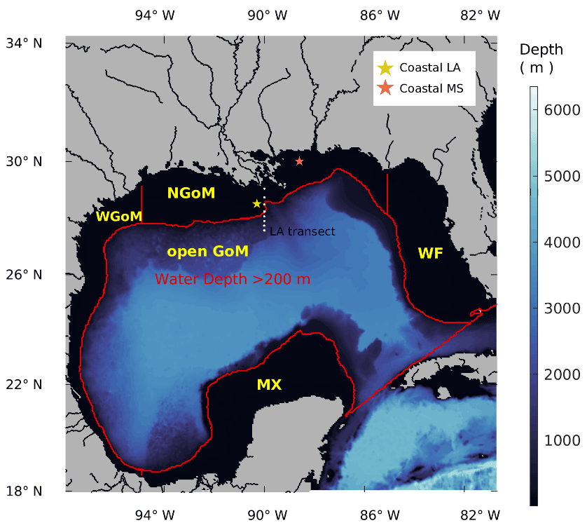
Figure 1 Gulf-COAWST model domain with water depth in color (unit: m). Subregional definitions follow Xue et al. (2016), which are the Mexico shelf (MX), western Gulf of Mexico shelf (WGoM), northern Gulf of Mexico shelf (NGoM), western Florida shelf (WF), and open GoM.

The revised biogeochemical model incorporates key processes regulating the carbon model, including primary production, river DIC, PON and DOC delivery, sediment carbon burial, CO₂ air–sea flux, CaCO₃ cycling, and OM remineralization (Fig. 2). Widely used carbon system variables, such as pCO₂, pH, and Ω, are used as carbon system state indicators. The carbon module that takes in DIC, TA, PO₄, Si (dissolved inorganic silicon), salt, and temperature for calculating pCO₂, pH, Ω_Arag, and Ω_Calc largely follows the recommended best practices (Dickson et al., 2007; Eyring et al., 2016; Orr et al., 2017; Zeebe and Wolf-Gladrow, 2001), with an updated parameter prescription for dissociation constants for carbonic acid (K₁) and the bicarbonate ion (K₂) (Millero, 2010), as well as solubility products for aragonite K_A and calcite K_C (Mucci, 1983) with a pressure effect (Millero, 1982, 2007).

The inorganic carbonate mineral (mainly CaCO₃) forms during the photosynthetic activities of some phytoplankton species and fosters aggregation of detritus and their sinking. The rate of CaCO₃ production follows a dynamic ratio regarding the primary production of small phytoplankton with low-temperature inhibition and enhancement during bloom conditions (Moore et al., 2004). The production and dissolution of CaCO₃ are important processes for ocean acidity regulation, as its production (by 1 unit) nominally takes away a unit of [CO${}_{\mathrm{3}}^{\mathrm{2}-}$] from water, which reduces the alkalinity and DIC by 2 units and 1 unit, respectively. This process routinely happens during photosynthetic activities of some phytoplankton species (such as coccolithophores, parameterized implicitly as a portion of small phytoplankton in this model) and other marine calcifiers. Carbonate minerals produced in the euphotic zone could be treated as equivalent storage of alkalinity and are usually transported towards the ocean sediment through sinking. Aragonite and calcite are two common mineral phases of CaCO₃ secured by marine organisms and are included in the model. Ω_Calc and Ω_Arag are calculated as the equilibrium product of Ca²⁺ and CO${}_{\mathrm{3}}^{\mathrm{2}-}$. When Ω>1, calcification is thermodynamically favored, and when Ω<1, dissolution is thermodynamically favored. In Eq. (1), [Ca²⁺] and [CO${}_{\mathrm{3}}^{\mathrm{2}-}$ ] are the concentrations of calcium and carbonate ions, respectively. [Ca²⁺] is determined through salinity (Millero, 1982, 1995), and [CO${}_{\mathrm{3}}^{\mathrm{2}-}$] is calculated through the carbon module. K_sp is the stoichiometric solubility product dependent on pressure, temperature, and salinity. K_sp is defined for aragonite and calcite as K_A and calcite K_C, respectively.

$$\begin{array}{}\text{(1)}& \mathrm{\Omega }={\displaystyle \frac{\left[{\mathrm{Ca}}^{\mathrm{2}+}\right]\left[{\mathrm{CO}}_{\mathrm{3}}^{\mathrm{2}-}\right]}{K_{\mathrm{sp}}}}\end{array}$$

In our model, the sediment pool of sinking particles is a simplified representation of burial and benthic remineralization processes, whereby the flux of sinking materials out of the bottommost grid point is added to the sediment pool and enters the burial pool (remains inactive) with a dynamic ratio, the active sediment pools undergo enzyme-aided decomposition at rates regulated by temperature and oxygen and then release a corresponding influx of ammonium, DIC, and alkalinity at the sediment–water interface. Our model uses a CO₂ production ratio of 0.138 between sediment aerobic respiration and denitrification (Fennel et al., 2006) and an alkalinity production ratio of 1.93 between pyrite burial and denitrification (Hu and Cai, 2011). Upon being sunk to acidified regions, the dissolution of CaCO₃, regulated by Ω, can consume dissolved CO₂ and neutralize the acid.

The bulk formula for air–sea gas exchange for CO₂ is used following Wanninkhof (1992). Air–sea CO₂ flux is calculated with a time step of 240 s and output in the form of a daily average. The gas transfer velocity coefficient of 0.31 cm h⁻¹ is used in Eq. (2).

$$\begin{array}{}\text{(2)}& F_{{\mathrm{CO}}_{\mathrm{2}}}=k_{\mathrm{660}}{\left({\displaystyle \frac{Sc}{\mathrm{660}}}\right)}^{-\mathrm{1}/\mathrm{2}}s\mathrm{\Delta }p{\mathrm{CO}}_{\mathrm{2}}\end{array}$$

where $F_{{\mathrm{CO}}_{\mathrm{2}}}$ is the air–sea CO₂ flux (in mmol CO₂ m⁻² d⁻¹), Sc is the Schmidt number (nondimensional) (calculated following Wanninkhof, 2014), s is the solubility of CO₂ in seawater (in mol CO₂ m⁻³ µatm⁻¹) (calculated following Weiss, 1974), and ΔpCO₂ is the air–sea pCO₂ difference (in µatm). The term k₆₆₀ is the quadratic gas transfer coefficient in cm h⁻¹ (converted to m d⁻¹). We calculated the air–sea CO₂ flux using the relationships of gas exchange with wind speed at 10 m over the sea surface (U₁₀), following Wanninkhof (1992). We used the ocean convention for the CO₂ flux; i.e., a positive flux is defined as the ocean being a sink of atmospheric CO₂. Air pCO₂ level is prescribed using a fitted curve from the column-averaged dry-air mole fraction of atmospheric carbon dioxide from 2002 to the present derived from a satellite product (merged dataset from SCIAMACHY/ENVISAT, TANSO-FTS/GOSAT, and OCO-2, https://cds.climate.copernicus.eu/, last access: 24 May 2021; Dils et al., 2014).

Figure 2 Schematic plot showing major processes incorporated in the carbon cycle.

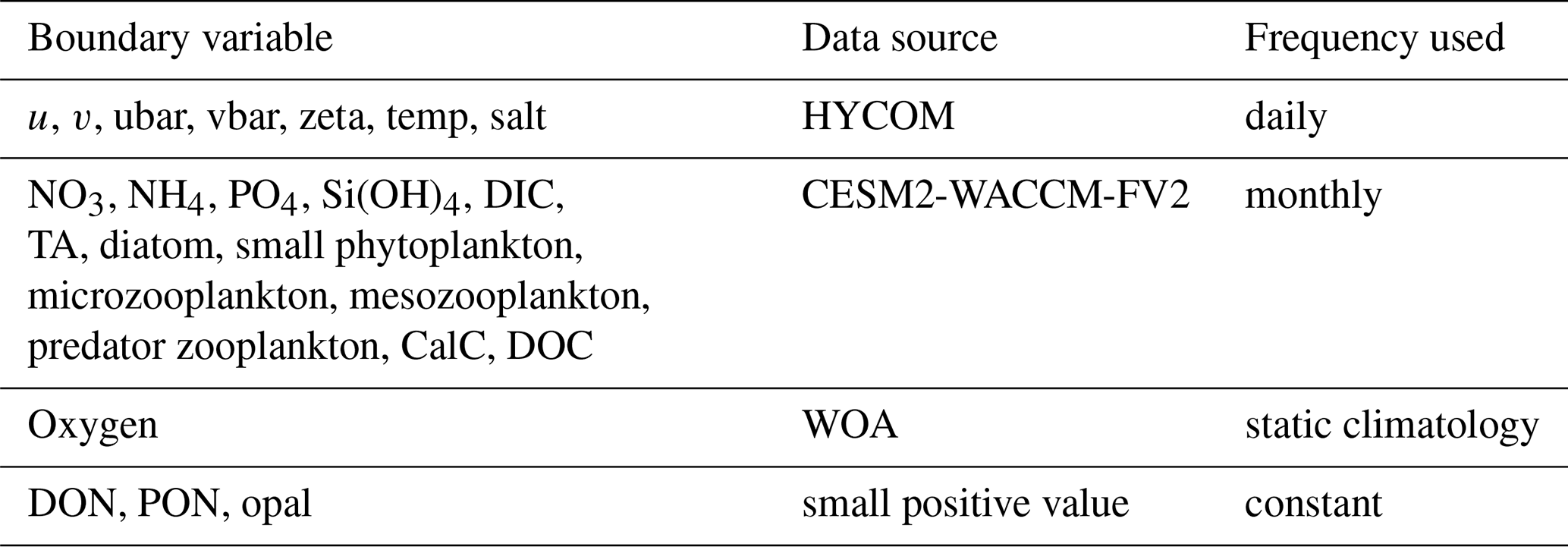
We performed a 20-year model hindcast covering the period of 1 January 2000 to 31 December 2019. The physical model setup was similar to that of Zang et al. (2020), with ocean physical initial and boundary conditions interpolated from the $\mathrm{1}/\mathrm{12}{}^{\circ }$ data-assimilated Hybrid Coordinate Ocean Model (HYCOM/NCODA, GLBu0.08/expt_19.1, expt_90.9, expt_91.0, expt_91.1, expt_91.2, and GLBv0.08/expt_93.0, https://www.hycom.org, last access: 27 September 2021; Chassignet et al., 2003, 2013). Physical boundary conditions are of daily frequency and include u, v, ubar, vbar, zeta, temperature, and salt. Atmospheric forcings with 6-hourly frequency include ground-level or sea surface downwelling shortwave and longwave radiation, ground-level or sea surface upwelling shortwave and longwave radiation, surface air pressure, surface air temperature, relative humidity, precipitation, wind at 10 m. They were extracted from the NCEP Climate Forecast System Reanalysis (CFSR) (Saha et al., 2010) and Climate Forecast System Version 2 (CFSv2) (Saha et al., 2011). See Table A2 for a list of model forcing frequencies.

The Coupled Model Intercomparison Project 6 (CMIP6) participating GCMs consume enormous research resources and generate unprecedented knowledge on global carbon system evolution with a whole-ecosystem conservation perspective (Bentsen et al., 2019; Bethke et al., 2019; Boucher et al., 2021, 2018; Danabasoglu, 2019a, b; Danabasoglu, 2019c, d; Guo et al., 2018; Jungclaus et al., 2019; Krasting et al., 2018; Lovato et al., 2021; Neubauer et al., 2019; Seland et al., 2019; Swart et al., 2019; Wieners et al., 2019; Ziehn et al., 2019). Utilizing GCMs results in a refined regional model that extends their research value, especially in bridging coarse GCM products with in situ field observations. With the interannual variation estimated by GCMs, the regional model could take advantage of global models by using dynamic boundaries that reflect climate oscillations and carbon accumulation in oceanic waters. In this study, we carefully evaluate various GCM products as candidates for initial and boundary conditions for the biogeochemical model. The two prognostic variables dissolved inorganic carbon (DIC) and total alkalinity (TA) are the essential data needed to drive a regional oceanic carbon model. There are no time-varying observational products or reanalysis of DIC and TA that have ideal three-dimensional coverage of the GoM. NCAR's CESM2-WACCM-FV2 solution was chosen to serve as the model boundary due to its relatively small bias in the carbonate variables in the GoM, relatively high horizontal resolution in the GoM compared with other GCMs, and availability of nutrients and carbon variables (see Table A1 for more details). Monthly boundary conditions of the biogeochemical variables (DIC, DOC, TA, NO₃, PO₄, Si, NH₃) are extracted from CESM2-WACCM-FV2 solutions (historical, r1i1p1f1, nominal resolution 100 km, Danabasoglu, 2019b). As the global model simulation ended in December 2014, the biogeochemical boundary condition of 2014 was used repeatedly for the period from 2015 to 2019. The oxygen boundary condition is static without temporal changes since O₂ is not available from the CESM2-WACCM-FV2 and is interpolated from the World Ocean Atlas 2018 (WOA18) product (Boyer et al., 2018; García et al., 2019). Freshwater and terrestrial nutrient inputs from 47 major rivers discharged to the GoM are applied as point sources with daily frequency. River discharge and water quality data for rivers in the US are collected from the US Geological Survey (USGS) stations (https://maps.waterdata.usgs.gov, last access: 25 August 2020). River DOC is prescribed following the values reported by Shen et al. (2012), with additional references from several other studies (Reiman and Xu, 2019; Stackpoole et al., 2017; Wang et al., 2013; Xu and DelDuco, 2017). Mexican river discharge data are collected from BANDAS (https://www.gob.mx/conagua, last access: 25 December 2019). Water quality data for Mexican rivers are prescribed as the average of that of the Mississippi and Atchafalaya rivers. River nutrient and carbon load are reconstructed from available USGS observations (see Fig. 3 for time series of river DIC and TA input). Missing river alkalinity values are interpolated from climatological values, and missing river DIC values are calculated from pH and alkalinity using the MATLAB program CO2SYS (Lewis and Wallace, 1998). Validations of the model's performance in physics, nutrient cycle, and primary production can be found in Zang et al. (2019, 2020). In this study, we focus on the model's performance in the carbon cycle, which is presented in the next section.

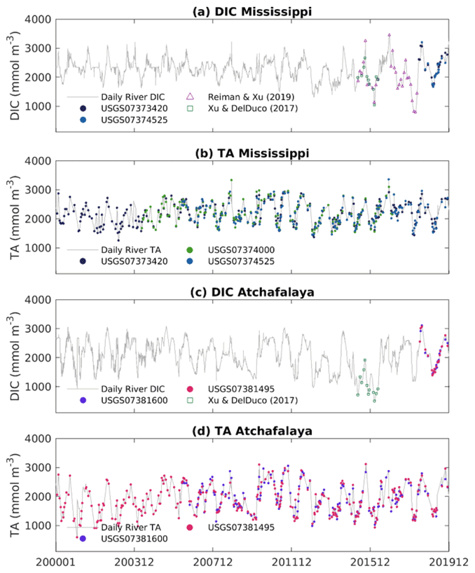
Figure 3 River DIC and TA concentration prescribed in the model. Grey lines are the interpolated daily concentration values; colored data points are raw data collected from multiple sources.

Since the model-simulated DIC concentration in the water column is sensitive to initial conditions (Hofmann et al., 2011; Xue et al., 2016), using the initial condition from a snapshot (January 2000) of the global model result would be appropriate as the global model has been well stabilized up to the year 2000 from its “pre-industry” experiment. The regional model has the benefit of swift spin-up, with the biogeochemical model typically completing its spin-up in 1 year (e.g., Große et al., 2019; Laurent and Fennel, 2019; Laurent et al., 2021). We conducted a series of sensitivity tests and confirmed that a 1-year spin-up period (the year 2000) is sufficient for our current model setup. All results presented below are based on model outputs from 2001 to 2019 unless otherwise specified. To quantify the impact of river discharge and the global ocean on the carbon system in the GoM, in addition to the control experiment wherein the historical product of the CESM2-WACCM-FV2 experiment is applied as the boundary conditions (from here, experiment “His”), two perturbed experiments, “Bry” and “NoR”, are added. The Bry experiment has clamped DIC and TA conditions as those of the year 2000 for all following years while keeping all other experiment setups the same as that of the His. The NoR experiment eliminates the presence of all rivers in the model while keeping the rest of the experiment setup the same as that of the His. As most available observations are confined to the surface ocean, except for the GOMECC transects, for this study we focus on the surface ocean carbon condition in the NGoM and open GoM waters.

3 Validation

This section focuses on the validation of the model results via comparison against autonomous mooring systems with surface pCO₂ measurements, ship-based measurements from the Gulf of Mexico Ecosystems and Carbon Cruise transects (GOMECC, Barbero et al., 2019; Wanninkhof et al., 2013, 2016), and pCO₂ underway measurements (data downloaded from https://www.ncei.noaa.gov/access/oads/, last access: 15 August 2021). Direct observations of the GoM carbon system have been recognized as unbalanced among seasons due to fewer data points available in winter compared to other seasons. To overcome the sporadic direct measurement dataset, we also performed a model–data comparison against the remote-sensing-based ML product of sea surface pCO₂ by Chen et al. (2019).

3.1 Model–buoy comparisons

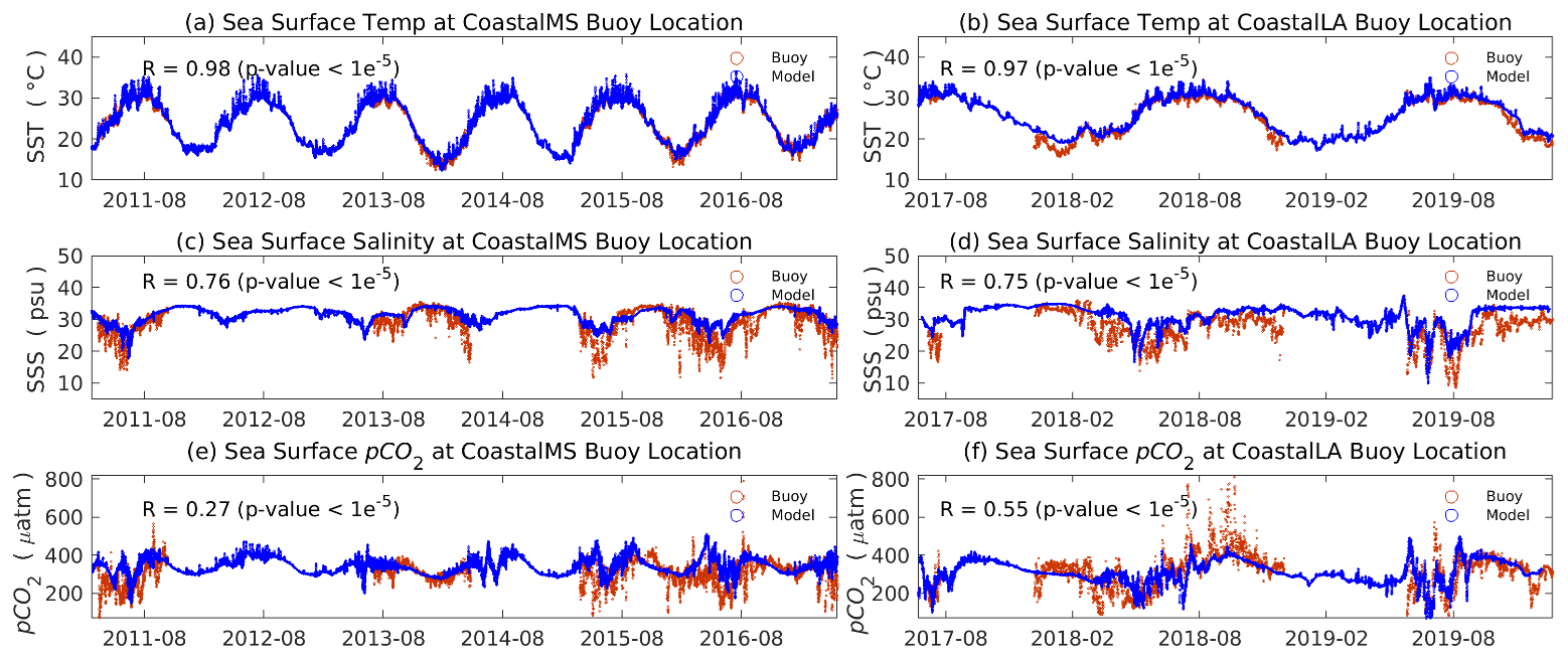
Temporal variability of sea surface pCO₂ was recorded by the autonomous mooring system at two sites (CoastalMS and coastal LA) operated by the Atlantic Oceanographic and Meteorological Laboratory (AOML) of the National Oceanic and Atmospheric Administration (NOAA). The CoastalMS buoy site (for location see Fig. 1, data coverage: 14 January to 9 December 2009; 17 March 2011 to 4 August 2012; 10 July 2013 to 10 February 2014; 10 February to 3 May 2014; 12 December 2014 to 22 March 2015; 30 March 2015 to 22 September 2016; 23 September 2016 to 29 May 2017) is predominately impacted by the Mississippi River followed by the coastal ocean, whereas the CoastalLA buoy site (data coverage: 14 July to 7 November 2017; 14 December 2017 to 26 April 2019; 4 June 2019 to 12 August 2020; 12 August 2020 to 25 August 2021; 25 August to 29 November 2021) is mutually influenced by the Mississippi River and the coastal ocean. The high-frequency measurements provide a time-resolved picture of year-round changing pCO₂ values. Temperature and salinity can influence the chemical equilibrium in the carbonate system, therefore shifting the pCO₂ values. Validating the temperature and salinity at these two mooring sites is a prerequisite before looking into the surface pCO₂ levels. In Fig. 4, the top four panels compare the sea surface temperature (SST) and salinity (SSS) between model and buoy measurements and show satisfying model–data agreements, with correlation coefficients larger than 0.75. At CoastalMS, the range for sea surface pCO₂ is 150∼ 600 µatm. Sea surface pCO₂ records are more volatile at CoastalLA with a maximum value >800 µatm and a minimum value around 150 µatm. Following the salinity drop, pCO₂ at the CoastalMS site is simultaneously reduced, demonstrating the river's influence on both salinity and pCO₂. At CoastalLA, however, the pCO₂ level does not necessarily follow the trend of salinity, implying complex controlling factors in addition to the river inputs. The bottom two panels of Fig. 4 show acceptable agreement between measured and simulated sea surface pCO₂, with a correlation coefficient of 0.27 between modeled and observed surface pCO₂ at the CoastalMS buoy location and a correlation coefficient of 0.55 between modeled and observed surface pCO₂ at the CoastalLA buoy location. We notice model–data discrepancies in April 2018 at CoastalLA and July 2011 at CoastalMS and ascribe such bias to the uncertainty in the riverine DIC input prescription and the limited model horizontal resolution (∼ 5 km).

Figure 4 Time series of SST, SSS, and pCO₂_sea at sites CoastalLA and CoastalMS.

3.2 Model–cruise comparisons

Cruise carbon measurements include underway water pCO₂ data and conductivity–temperature–depth (CTD) bottle results. We compare the model result at the LA transect with the observations of GOMECC cruises conducted at the same location during GOMECC1 in 2007, GOMECC2 in 2012, and GOMECC3 in 2017. Measurements of TA during GOMECC cruises followed Dickson's definition (1981), wherein the TA is expressed as Eq. (3).

$$\begin{array}{}\text{(3)}& \begin{array}{rl}\mathrm{TA}& =\left[{\mathrm{HCO}}_{\mathrm{3}}^{-}\right]+\mathrm{2}\left[{\mathrm{CO}}_{\mathrm{3}}^{\mathrm{2}-}\right]+\left[B{\left(\mathrm{OH}\right)}_{\mathrm{4}}^{-}\right]+\left[{\mathrm{OH}}^{-}\right]\\ & +\left[{\mathrm{HPO}}_{\mathrm{4}}^{\mathrm{2}-}\right]+\mathrm{2}\left[{\mathrm{PO}}_{\mathrm{4}}^{\mathrm{3}-}\right]+\left[{\mathrm{H}}_{\mathrm{3}}{\mathrm{SiO}}_{\mathrm{4}}^{-}\right]+\left[{\mathrm{NH}}_{\mathrm{3}}\right]\\ & +\left[{\mathrm{HS}}^{-}\right]-\left[{\mathrm{H}}^{+}\right]-\left[{\mathrm{HSO}}_{\mathrm{4}}^{-}\right]-\left[\mathrm{HF}\right]\\ & -\left[{\mathrm{H}}_{\mathrm{3}}{\mathrm{PO}}_{\mathrm{4}}\right]-\left[{\mathrm{HNO}}_{\mathrm{2}}\right]\end{array}\end{array}$$

Equation (3) contains 14 variables, among which $\left[{\mathrm{PO}}_{\mathrm{4}}^{\mathrm{3}-}\right]$ is explicitly modeled as an active tracer, $\left[{\mathrm{HCO}}_{\mathrm{3}}^{-}\right]$, $\left[{\mathrm{CO}}_{\mathrm{3}}^{\mathrm{2}-}\right]\left[B{\left(\mathrm{OH}\right)}_{\mathrm{4}}^{-}\right]$, [OH⁻], $\left[{\mathrm{HPO}}_{\mathrm{4}}^{\mathrm{2}-}\right]\left[{\mathrm{H}}_{\mathrm{3}}{\mathrm{SiO}}_{\mathrm{4}}^{-}\right]$, [H⁺], [HF], [H₃PO₄], and $\left[{\mathrm{HSO}}_{\mathrm{4}}^{-}\right]$ are calculated by the carbon module, and [HS⁻], [HNO₂], and [NH₃] are unaccounted for. Figure 5 shows the vertical profiles of observed DIC, TA, and their ratio collected at the LA transects (−90^∘ W, 27.5–29.1^∘ N, shown in Fig. 1) overlaid with the model solution; the top 200 m depth is stretched three times to have a better view of the more densely sampled observational data, and a black dot is placed in the location of each observational data point, with the oversized colored dot representing the value of the measurement. All three transects were taken during July when nutrient supply from the MARS was high. Model-simulated profiles at the transects are taken from the closest date of the daily averaged output. The general trends in Fig. 5 for DIC, TA, and their ratio demonstrate a good match between the model result and the in situ CTD data. A relatively low surface DIC concentration (<2150 mmol m⁻³) above the 200 m isobath demonstrates the river's influence at the NGoM. The general increasing trend of DIC with depth confirms the presence of a biological pump, whereby inorganic carbon is utilized during photosynthesis in the euphotic layer. Subsequently, the generated OM sinks into deeper waters while being remineralized along the way. The TA profiles show more variation compared with DIC, for which a lower TA concentration (<2380 milliequivalents m⁻³) could generally be found at the surface as the direct dilution from river discharge, followed by a quick increase to ∼ 2380 milliequivalents m⁻³ in the euphotic layer due to photosynthetic activities, which generate alkalinity. Deeper, the TA profiles show a decreasing trend between 200 and 700 m, which could be explained by the water column respiration and nitrification. The TA profiles show a slow increase from 800 m and deeper, which coincides with the alkalinity generation processes in sediment and possibly dissolution of carbonate minerals, both adding to the bottom water TA. The TA $/$ DIC ratio has a maximum at the surface due to low DIC concentration and decreases with depth as DIC concentration increases. The last column in Fig. 5, namely (d), (h), and (l), quantifies the difference between the model solutions as well as the observations and the distribution of the difference. Figure 5d shows that 51.2 % of model–obs difference for DIC is within [$-\mathrm{10},\mathrm{10}$] µmol kg⁻¹. Similarly, Fig. 5h shows that 49.8 % of model–obs difference for TA is within [$-\mathrm{10},\mathrm{10}$] µmol kg⁻¹, and Fig. 5l shows that 91.6 % of model–obs difference for the TA $/$ DIC ratio is within [−0.02 0.02]. The model's root mean square error (RMSE) for DIC, TA, and the TA $/$ DIC ratio over the GOMECC (2007–2017) LA transect dataset is 30.97, 26.86, and 0.014, respectively.

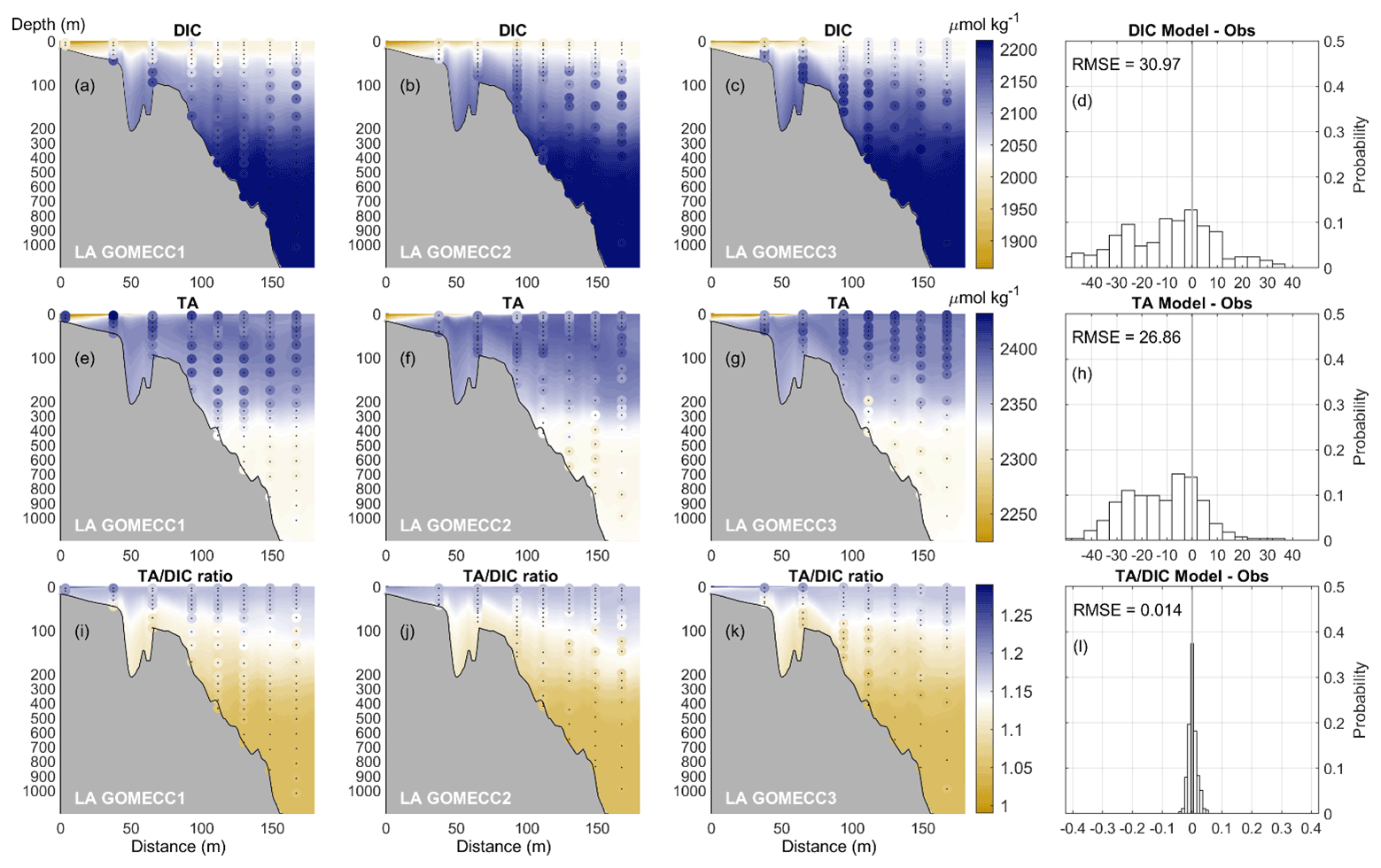
Figure 5 Discrete measurement of DIC and TA along the LA transect during GOMECC1, GOMECC2, and GOMECC3 cruises shown as oversized scattered dots (with the little black dots indicating their locations) compared with model results in color contour, with the water depth shown on the left side of each figure in meters. The distributions of model bias and RMSE for DIC, TA, and the TA $/$ DIC ratio combining the three GOMECC cruises at the LA transect are shown in (d), (h), and (l), respectively.

3.3 Model–ML pCO₂ product comparisons

Direct comparison between cruise measurements of ocean surface pCO₂ and daily averaged model results might suffer from systematic bias due to the sparsity of cruise data, both temporally and spatially. The ML model generates surface pCO₂ from Chen et al. (2019) integrated >220 cruise surveys for 2002–2019 and MODIS ocean color product covering 2002–2017. The comparison between the two surface pCO₂ products is shown in Fig. 6, where surface pCO₂ results from Chen et al. (2019) are denoted as “ML” and results from this work are denoted as “Model” for the monthly climatology from July 2002 to December 2017. The two results exhibit a similar spatial distribution of surface pCO₂, with our model result revealing more dominant features from the Loop Current in the open ocean. Compared with the ML model, our model produces lower pCO₂ estimates over NGoM during winter and fall, higher pCO₂ estimates over WF during summer, and a stronger influence from the Caribbean Sea. Chen et al. (2019) reported that no satellite data were found for pCO₂<145 µatm or >550 µatm during their model development. This can also be a factor when considering the differences between the two products. Further comparison between our model and other products can be found in Sect. 5.1.

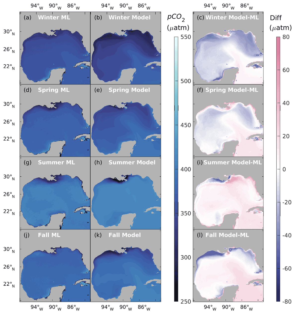
Figure 6 Comparison of surface pCO₂ between the ML model (Chen et al, 2019) and this work.

Besides buoy records, transects, and the ML products, we also perform an extensive model–data comparison using available ship-based underway pCO₂ measurements from the Ocean Carbon and Acidification Dataset (https://www.ncei.noaa.gov/access/oads/, last access: 12 October 2021). These extensive model–data comparisons give us confidence that our model, driven by carbon boundary conditions from the global model, can reproduce temporal, spatial, and vertical variability of the CO₂ dynamics in the GoM.

4 Result

In this section, we present the spatial and temporal pattern of key carbon system variables, namely pCO₂, pH, Ω, and air–sea CO₂ flux simulated over the past 20 years in the GoM. In this study, we emphasize the surface carbon condition in two regions: NGoM and the open GoM, where most existing in situ data are distributed. We perform a linear fit of the time series of the key carbon system variables in each region and show the fitted relationships in Fig. 7. The slopes of the fitted linear plot give estimations of the change rate of each carbon variable over the past 2 decades.

Figure 7 Time series and trend analysis of sea surface (a) pCO₂, (b) pH, and (c) Ω_Arag for the NGoM (blue) and open GoM (red). Solid lines depict the daily spatial mean value; shaded areas stand for 1 standard deviation, and dashed lines trace the linear fit of the time series.

4.1 pCO₂

We simulate a generally increasing trend in surface pCO₂ level for both NGoM and open GoM, with an increasing rate of 1.61 and 1.66 µatm yr⁻¹, respectively (Fig. 7). Seasonal ocean surface pCO₂ variation is primarily affected by temperature variations. To evaluate the pCO₂ trend without temperature effects, we decouple the thermal and nonthermal components of pCO₂ at the ocean surface using Eqs. (4) and (5) and further extract the pCO₂ variation due to gross primary production and air–sea CO₂ flux. The temperature sensitivity of CO₂ of γ_T=4.23 % per degree Celsius, proposed by Takahashi et al. (1993), is used to perform the thermal decoupling in Eqs. (4) and (5). The thermal effect on pCO₂ (pCO${}_{\mathrm{2}}^{\mathrm{th}}$) is defined as the deviation between apparent pCO₂ and the estimated pCO₂ at the mean SST (denoted as < SST >). The nonthermal counterpart (pCO${}_{\mathrm{2}}^{\mathrm{nt}}$) is obtained by removing the thermal effect from the pCO₂ time series using Eq. (5). Note that this definition of pCO${}_{\mathrm{2}}^{\mathrm{th}}$ is different from the original definition given by Takahashi et al. (2002). The new definition allows the thermal and nonthermal CO₂ components to sum up to the apparent pCO₂. pCO₂ variations due to gross primary production are estimated from the carbon module based on the DIC consumed by gross primary production and denoted as pCO${}_{\mathrm{2}}^{\mathrm{GPP}}$. pCO₂ variations due to air–sea CO₂ flux are calculated from the carbon module based on the DIC change from the air–sea exchange and denoted as pCO${}_{\mathrm{2}}^{\mathrm{flux}}$.

The contribution from gross primary production (GPP) is the process that directly affects the CO₂ uptake, and GPP can be calculated by tracking the photosynthesis activity of diatoms and small phytoplankton (which is a function of solar radiation, temperature, nutrients, and phytoplankton concentrations). Respiration, on the other hand, is more complicated to quantify since it concerns both living biota (phytoplankton, zooplankton) and nonliving detritus (PON, DOC). Both respiration at the surface and respiration that happens in deeper water as detritus sinks modify DIC concentration and create concentration gradients. We leave the respiration in the end-member of the pCO${}_{\mathrm{2}}^{\mathrm{nt}}$ components, which incorporated various mixing processes (e.g., river water and oceanic water mixing, vertical mixing of upwelled waters, horizontal-advection-induced lateral transport of tracers with concentration gradients, and entrainment of waters with different chemical nature – i.e., temperature, salt, DIC, TA, and detritus concentration). Remineralization and respiration are included in the term pCO${}_{\mathrm{2}}^{\mathrm{mixing}}$ due to the result of the two processes altering water chemical nature (DIC, TA, detritus concentration), and the impacts of water chemical nature on pCO₂ are constantly being modified by (and as a result of) the mixing process.

$$\begin{array}{}\text{(4)}& {\displaystyle }p{\mathrm{CO}}_{\mathrm{2}}^{\mathrm{th}}=p{\mathrm{CO}}_{\mathrm{2}}\cdot \left[\mathrm{1}-\exp \left({\mathit{\gamma }}_T\cdot \left(<\mathrm{SST}>-\mathrm{SST}\right)\right)\right]\text{(5)}& {\displaystyle }p{\mathrm{CO}}_{\mathrm{2}}^{\mathrm{nt}}=p{\mathrm{CO}}_{\mathrm{2}}\cdot \exp \left({\mathit{\gamma }}_T\cdot \left(<\mathrm{SST}>-\mathrm{SST}\right)\right)\text{(6)}& {\displaystyle }p{\mathrm{CO}}_{\mathrm{2}}^{\mathrm{nt}}=p{\mathrm{CO}}_{\mathrm{2}}^{\mathrm{GPP}}+p{\mathrm{CO}}_{\mathrm{2}}^{\mathrm{flux}}+p{\mathrm{CO}}_{\mathrm{2}}^{\mathrm{mixing}}\end{array}$$

Figure 8 shows the seasonal and spatial patterns of four decoupled pCO₂ components, namely pCO${}_{\mathrm{2}}^{\mathrm{th}}$, pCO${}_{\mathrm{2}}^{\mathrm{nt}}$, pCO${}_{\mathrm{2}}^{\mathrm{GPP}}$, and pCO${}_{\mathrm{2}}^{\mathrm{flux}}$. The pCO${}_{\mathrm{2}}^{\mathrm{th}}$ patterns in the second row (e, f, g, h) of Fig. 8 reflect the fluctuation of pCO₂ due to thermal effects. Over the four seasons, a general pattern of rising pCO${}_{\mathrm{2}}^{\mathrm{th}}$ from spring to summer and a gradual reduction from summer onwards can be observed. The NGoM shelf exhibits the lowest pCO${}_{\mathrm{2}}^{\mathrm{th}}$ values during winter, while WF shows elevated pCO${}_{\mathrm{2}}^{\mathrm{th}}$ values during summer. The higher pCO${}_{\mathrm{2}}^{\mathrm{th}}$ values in the southern part of the Yucatan shelf reveal the warm water flowing into the GoM from the Caribbean Sea. The top row (a, b, c, d) of Fig. 8 shows the nonthermal component of pCO₂. The relatively high pCO${}_{\mathrm{2}}^{\mathrm{nt}}$ during winter on the NGoM shelf, compared to that of the open GoM, shows the strong solvation effect of CO₂ with low SST, contributing to a high DIC $/$ TA ratio and strong carbon uptake.

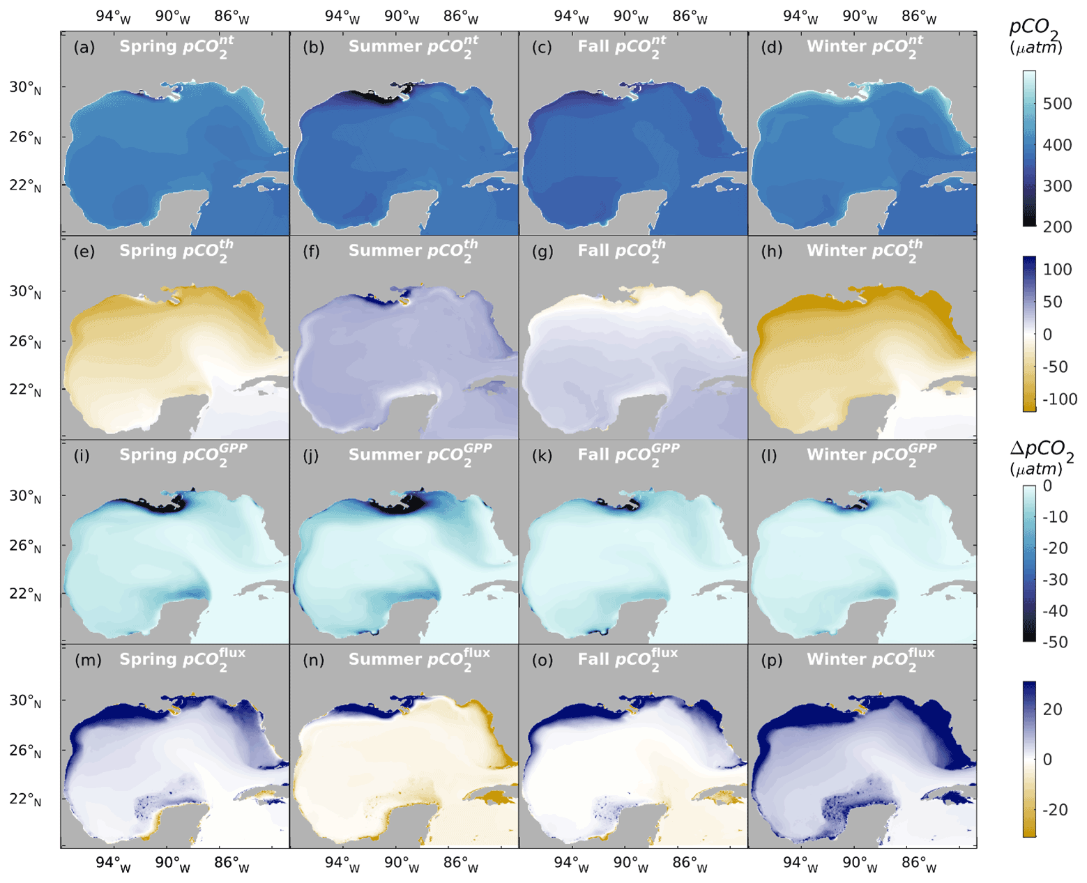
Figure 8 Spatial distribution of sea surface pCO₂ over four seasons. From the top to the bottom row: pCO${}_{\mathrm{2}}^{\mathrm{th}}$ (a through d), pCO${}_{\mathrm{2}}^{\mathrm{nt}}$ (e through h), pCO${}_{\mathrm{2}}^{\mathrm{GPP}}$ (i through l), pCO${}_{\mathrm{2}}^{\mathrm{flux}}$ (m through p; positive indicates the air–sea CO₂ flux works in the direction of increasing sea surface pCO₂).

The lower two rows of Fig. 8 show pCO₂ changes due to the gross primary production and CO₂ air–sea exchange, respectively. The pCO${}_{\mathrm{2}}^{\mathrm{GPP}}$ reflects the intensity of primary production in terms of pCO₂ reduction. pCO${}_{\mathrm{2}}^{\mathrm{GPP}}$ has larger magnitudes in NGoM during spring and summer and is gradually attenuated during and after fall. The large magnitudes of pCO${}_{\mathrm{2}}^{\mathrm{GPP}}$ during summer in NGoM waters and the open GoM region following the extension of the MARS plume suggest strong biological CO₂ removal in those regions. These results show that gross primary production has a stronger regulation on surface pCO₂ during spring and summer in river-dominated waters and upwelling regions. At the same time, a minor contribution from gross primary production can be seen during winter, on the flat and shallow WF, and in the open GoM regions south of the Loop Current.

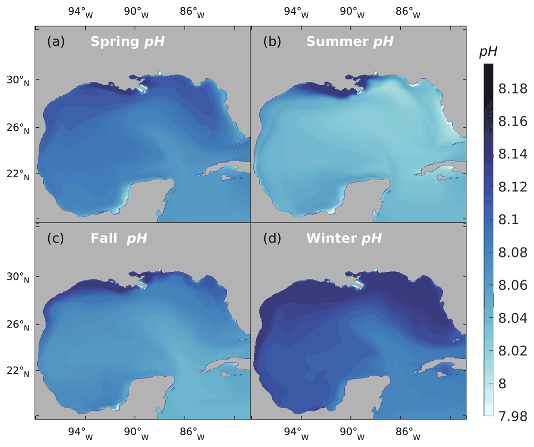
Figure 9 Seasonally averaged sea surface pH over 2001–2019.

The pCO${}_{\mathrm{2}}^{\mathrm{flux}}$ reflects the intensity of air–sea CO₂ exchange attempting to mitigate the disequilibrium caused by local physical and biological processes. The relatively high value of pCO${}_{\mathrm{2}}^{\mathrm{nt}}$ and low magnitude of pCO${}_{\mathrm{2}}^{\mathrm{GPP}}$, as well as low river discharge (minimal river water mixing) in the WF during winter, indicate a strong CO₂ uptake from the atmosphere due to low SST. This analysis agrees with the low pCO${}_{\mathrm{2}}^{\mathrm{th}}$ and high pCO${}_{\mathrm{2}}^{\mathrm{flux}}$ values in the WF during winter, as shown in Fig. 8d and p. Situations during seasons other than winter are more complicated due to biological activities and mixing. The Mississippi delta region has a high pCO${}_{\mathrm{2}}^{\mathrm{th}}$ value during summer; however, combined with the effects of mixing and strong primary production (large magnitude of pCO${}_{\mathrm{2}}^{\mathrm{GPP}}$), this region acts as a strong carbon sink that exhibits a high value of pCO${}_{\mathrm{2}}^{\mathrm{flux}}$ compensated from the atmosphere. Figure 8 demonstrates that most of the time during the year, the surface pCO₂ pattern is not dominated by a single factor but a combination of multiple controlling processes. The result of pCO₂ decomposition agrees with the current view of the pCO₂ dynamic and carbon uptake patterns in the GoM, which is strong carbon uptake during winter due to the thermal effect and high biological CO₂ drawdown during spring and summer under the riverine influence.

4.2 pH

Ocean surface pH in the GoM shows a clear decreasing trend, with a 0.0020 yr⁻¹ decrease over the NGoM region and a 0.0015 yr⁻¹ decrease over the open GoM region. Figure 9 shows the seasonal pattern of ocean surface pH over the GoM. Spatial and seasonal pH patterns show larger variation over the NGoM, especially on the inner shelf (depth <50 m). The pH level in the surface water is closely associated with temperature, photosynthetic activities, and water mixing. The high pH value on the NGoM shelf reveals the strong influence of riverine alkalinity export and nutrient-stimulated primary production. The lower pH values on the WF shelf during summer and the generalized greater pH values over NGoM during winter demonstrate the high pH sensitivity to SST. The upwelling region along the western Yucatan shelf shows reduced pH values all year-round compared with its surrounding waters. The upwelling along the WGoM slope has a similar effect of reducing and maintaining a relatively low pH, effectively forming a pH boundary between the shelf water and the open GoM. The open GoM is largely dominated by the warmer and lower-pH water from the Caribbean Sea throughout the year.

4.3 Aragonite and calcite saturation state

Aragonite undersaturation occurs ([CO${}_{\mathrm{3}}^{\mathrm{2}-}$] <66 µmol kg²) before calcite undersaturation ([CO${}_{\mathrm{3}}^{\mathrm{2}-}$] <42 µmol kg²) (Feely et al., 2022, 2009). As a result, Ω_Calc is approximately 50 % higher than Ω_Arag, and their spatial and seasonal variations are very similar, as shown in Fig. 10. Variations in temperature, alkalinity, and pCO₂ impose important controls on Ω_Arag. The multiyear variability of Ω_Arag at the ocean surface is shown in Fig. 7c. The NGoM region shows a smaller decreasing trend in Ω_Arag (0.0045 yr⁻¹) compared to that of the open GoM (0.0068 yr⁻¹). Note that the data in Fig. 7 do not include water from the shallow shelf waters (water depth <10 m); therefore, the trend in NGoM does not incorporate the condition in coastal estuaries. The spatial distribution of Ω_Arag across the GoM depicts a healthy level of Ω and a low risk of ocean acidification (Fig. 10). While the coastal ocean generally has a relatively high Ω level, some coastal locations warrant special attention when evaluating their tendency towards calcium mineral dissolution. These locations include coastal regions that experience a large load of riverine OM inputs (e.g., the Mississippi River delta in summer) and the upwelling regions that receive relatively higher-acidity water from the bottom ocean (e.g., west of Yucatan). These regions show significant Ω reductions compared to the surrounding waters and are potential victims of ocean acidification. The influence of the river on Ω is complex. On one hand, a high nutrient level of river discharge could stimulate a high photosynthetic rate, which consumes DIC and increases Ω. On the other hand, photosynthesis favors calcification, which consumes carbonate ions and reduces Ω. Therefore, Ω is subject to increase with stronger photosynthesis and decrease with stronger calcification. Hence, the magnitude of the overall effect will depend upon photosynthetic rates and the calcification rate. In this work, two phytoplankton groups are modeled, diatoms (silicifying) and small phytoplankton (implicitly including the calcifying coccolithophores, foraminifera, and dinoflagellates), of which only the small phytoplankton group has the potential to conduct calcification (Raven and Giordano, 2009). Besides being regulated by temperature and small phytoplankton concentration, the calcification rate also depends on the composition of the phytoplankton population. The small phytoplankton group has a survival advantage at relatively low nitrogen concentrations and could be grazed by two zooplankton groups (mesozooplankton and microzooplankton), whereas diatoms are more nutrient-demanding and can be grazed by three zooplankton groups (predator zooplankton, mesozooplankton, and microzooplankton). The competitive phytoplankton evolution shapes the relative rates between photosynthesis and calcification on the NGoM shelf during summer. The reduced Ω to the east of the Mississippi River delta is a combined result of high-DIC water entrained by Loop Current eddies west of the delta and an increased ratio of small phytoplankton in offshore waters.

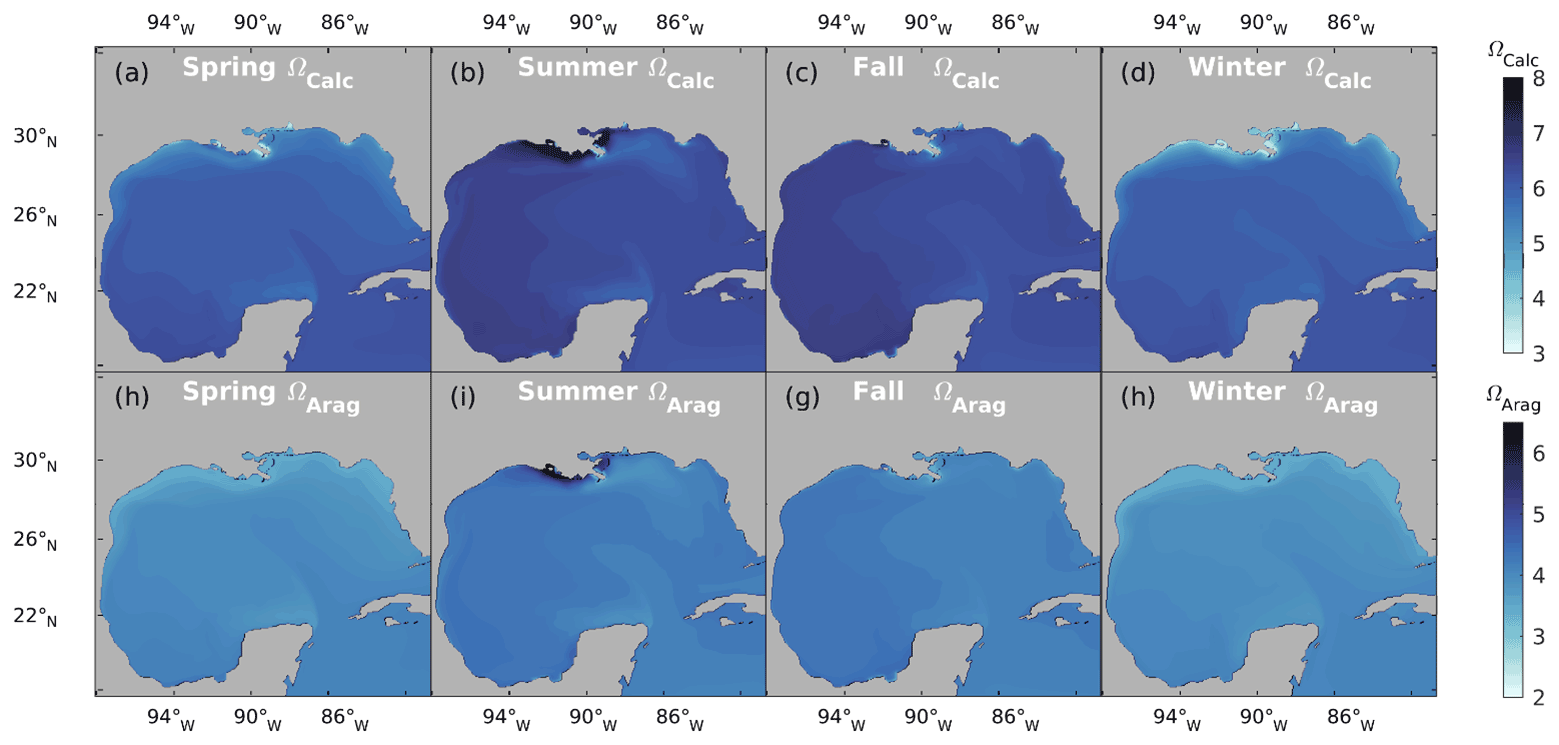
Figure 10 Seasonal mean sea surface Ω_Arag and Ω_Calc over 2001–2019.

4.4 Air–sea CO₂ flux

Air–sea CO₂ flux is calculated from daily averaged model data from 2001–2019 (Table 3). The GoM overall is a CO₂ sink with a mean flux rate of 0.62 mol C m⁻² yr⁻¹ (11.77 Tg C yr⁻¹), which is commensurate with the reported value of 11.8 Tg C yr⁻¹ by Coble et al. (2010). The greatest carbon uptake rate occurs in winter (1.97 mol C m⁻² yr⁻¹), while the weakest carbon uptake is present in fall (0.16 mol C m⁻² yr⁻¹). The strongest carbon efflux is simulated in summer (−0.57 C m⁻² yr⁻¹). On average, water in the NGoM acts as a sink throughout the year, and the water in the open GoM acts as a weak source during summer (and fall for 2002, 2004, 2006, and 2009) and a sink during the rest of the year. The direction and magnitude of the air–sea exchange can be seen in Fig. 11, where a positive number indicates that the ocean is a carbon sink. The NGoM is a very strong CO₂ sink year-round, and the open GoM is a source of CO₂ during summer but a sink in the rest of the year (except during fall in a few years), as shown in Fig. 11b. There are clear trends and patterns in multiyear CO₂ air–sea flux, as shown in Fig. 11a, where a greater air–sea CO₂ flux average could be seen at the end of 2019 than that of 2001, resulting in a stronger carbon influx in both regions. A significant anomaly in the middle part of the record (2009–2011) can be observed, which could result from the influence of a large negative North Atlantic Oscillation (NAO) index and El Niño in 2010 (Buchan et al., 2014). Similar observations in the Caribbean Sea are attributed to the single-year anomalies in the climate indices and the climate mode teleconnection (Wanninkhof et al., 2019).

Figure 11 Air–sea CO₂ exchange over the GoM: (a) multiyear CO₂ flux regression over the weekly mean levels in NGoM and open GoM; (b) seasonal CO₂ air–sea exchange budget over 2 decades in NGoM and open GoM.

4.5 Contribution from river and global ocean

In this section, we further diagnose river discharge and the global ocean's impacts on the GoM carbon system via a comparison between the control experiment (His) and the two perturbed experiments (Bry and NoR). In the Bry experiment the clamped boundary conditions that maintain the DIC and TA level as that of the year 2000, and in the NoR experiment the river forcing was removed to examine the impact of fluvial input on the coastal carbon system.

Figure 12 shows the multiyear mean levels of the four carbon variables (pCO₂, pH, Ω_Arag, and CO₂ flux) simulated by the three experiments. Table 1 summarizes the mean levels of pCO₂ over the NGoM and open GoM. The definition of pCO${}_{\mathrm{2}}^{\mathrm{th}}$, pCO${}_{\mathrm{2}}^{\mathrm{nt}}$, pCO${}_{\mathrm{2}}^{\mathrm{GPP}}$, pCO${}_{\mathrm{2}}^{\mathrm{flux}}$, and pCO${}_{\mathrm{2}}^{\mathrm{mixing}}$ can be found in Sect. 4.1. The pCO${}_{\mathrm{2}}^{\mathrm{mixing}}$ is defined in Eq. (6), which reflects the pCO₂ level due to the water mixing. It can also be considered the pCO₂ level determined by the water with a multiyear mean temperature and without the influence of gross primary production or air–sea CO₂ flux.

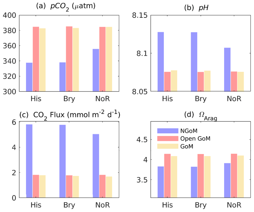
Figure 12 Multiyear synoptic of sea surface pCO₂, pH, CO₂ air–sea flux, and Ω_Arag with His, Bry, and NoR experiments. Color bars show the corresponding mean level from 2001 to 2019. Color legend: blue – NGoM, red – open GoM, yellow – GoM-wide. The units for pCO₂, pH, CO₂ flux, and Ω_Arag are µatm, unitless (full scale), mmol m⁻² d⁻¹, and unitless, respectively (note that the CO₂ air–sea flux used the ocean convention, with a positive value indicating transport from air to sea; i.e., the ocean is a sink).

The most salient difference among the three experiments is the significant elevation of the annual mean pCO₂ level (in Fig. 12) in the NGoM by the NoR experiment, combined with a significantly reduced carbon sink during summer (in Fig. 13, from 0.287 to −0.093 Tg per season using His as a benchmark). The difference can be better resolved by the pCO₂ decomposition results shown in Table 1, where a drastic change in the water carbon system emerges in the NGoM during the NoR experiment (compared to the other experiments with river input), evidenced by the large pCO${}_{\mathrm{2}}^{\mathrm{mixing}}$ value deviating from that of the His and Bry experiment in the NGoM region during spring, summer, and winter. The low values of pCO${}_{\mathrm{2}}^{\mathrm{nt}}$ in NGoM during summer can be explained by a strong biological drawdown of CO₂ associated with the high productivity fueled by the riverine nutrient supply. pCO${}_{\mathrm{2}}^{\mathrm{GPP}}$ components of −35.35 and −35.46 µatm, corresponding to the strong biological drawdown of CO₂ in Bry and His experiments, are in sharp contrast to that of the NoR experiment, which is only −3.10 µatm. Consequently, distinct patterns of CO₂ air–sea flux are shown in Fig. 13, and highly contrasting CO₂ air–sea-flux-induced surface pCO₂ changes are shown in Table 1 (pCO${}_{\mathrm{2}}^{\mathrm{flux}}$). The summer pCO${}_{\mathrm{2}}^{\mathrm{flux}}$ component for NGoM of the two experiments with river inputs exhibits a relatively large value (∼ 43 µatm) compared with that of the NoR experiment (0.2 µatm), demonstrating a much smaller disequilibrium between oceanic and atmospheric pCO₂ when rivers are absent. The changes introduced by removing the river showcase the dominating impact of river input on the NGoM carbon system in terms of gross primary production, surface pCO₂ level, and air–sea CO₂ exchange. Due to the different intensities of gross primary production, in the His experiment sediment PON concentration is 6 times that of the NoR experiment, and riverine nutrients in His fostered a ∼ 105 times higher PON burial rate in NGoM sediments than that of NoR.

Table 1 show a close resemblance in the magnitude and seasonal pattern between the Bry and His experiment in the open GoM region, with a small yet steady reduction in pCO${}_{\mathrm{2}}^{\mathrm{mixing}}$ by the Bry experiment among all seasons. The small reductions in pCO${}_{\mathrm{2}}^{\mathrm{mixing}}$ of the Bry experiment compared to that of His reflect the contribution from extraneous carbon accumulation from the global ocean that is included in the His experiment. As expected, slightly greater CO₂ sink values are reported in Fig. 13 for Bry than His. Since the Bry experiment has a smaller carbon accumulation in the open GoM region compared to that of the His experiment, the ocean surface requires a slightly greater carbon uptake to reach equilibrium with the atmosphere. Since oceanic water is a natural buffer system and the ocean surface is under constant interaction with the atmosphere, it is reasonable that the His and Bry experiments do not show significant differences in surface carbon variables. However, this does not mean that the accumulative signal of DIC from the global ocean is neglectable. As shown in Fig. 14, the ocean water equilibrium witnessed migration over the 20-year simulation. Compared with the Bry experiment, the His experiment received accumulated carbon input from the global ocean and underwent a [CO${}_{\mathrm{3}}^{\mathrm{2}-}$] reduction as large as 15 % in some affected regions at the 100 m depth. Combining the results from the three experiments, we conclude that, in addition to elevated atmospheric CO₂ levels, inputs from both MARS and global oceans contribute to the overall acidification trend in GoM, with the impacts from MARS mainly limited to the NGoM shelf region and the global ocean's impacts spanning the open GoM.

Table 1 Sea surface pCO₂ decomposition among experiments.

5 Discussion

In this study, we demonstrate that the regional high-resolution carbon model can reproduce the spatial and seasonal patterns of ocean surface pCO₂ in the GoM and generate reliable TA $/$ DIC profiles in the NGoM shelf. We detect a consistent acidification trend in the GoM over the past 2 decades. In this section, we present a side-by-side evaluation of the regional model with GCMs, global climatology products, and other regional models, followed by an envisioning of the future outlook and model development.

5.1 Model performance

In this section, we further evaluate the performance of our model via comparison against different global and regional models, as well as climatological products. The GoM region has limited observations of dissolved inorganic carbon (DIC) and total alkalinity (TA), and observational data covering different depths are even fewer. Due to lack of observations, global climatology products either have no coverage in the GoM region, e.g., mapped observation-based oceanic DIC monthly climatology from the Max Planck Institute for Meteorology (MOBO-DIC_MPIM) (NCEI Accession 0221526) (Keppler et al., 2020), or only contain surface carbon variables, e.g., the global gridded dataset of the surface ocean carbonate system called OceanSODA-ETHZ (v2021,NCEI Accession 0220059) (Gregor and Gruber, 2020), climatological distributions of pH, pCO₂, total CO₂, alkalinity, and CaCO₃ saturation in the global surface ocean (NCEI Accession 0164568) (Takahashi et al., 2017), the partial pressure of carbon dioxide collected from surface underway observations in the worldwide oceans (NCEI Accession 0161129) (Bakker et al., 2017), an observation-based global monthly gridded sea surface pCO₂ product (NCEI Accession 0160558) (Landschützer et al., 2017), and a global ocean pCO₂ climatology combining open-ocean and coastal areas (NCEI Accession 0209633) (Landschützer et al., 2020). The most updated global monthly TA (NCEI Accession 0222470) (Broullón et al., 2020b) and DIC (NCEI Accession 0222469) (Broullón et al., 2020a) products offer a 12-month climatology with a $\mathrm{1}{}^{\circ }\times \mathrm{1}{}^{\circ }$ spatial resolution and 102 vertical levels. Nevertheless, these products utilize a neural network approach to achieve three-dimensional coverage. Thus, one should be cautious that the generated monthly climatology products are not built solely from the interpolation of observations (Cervantes-Díaz et al., 2022). Rather, they are machine learning products with many untested assumptions. For instance, they use pCO₂ from LDEOv2016 (Takahashi et al., 2017) and TA from Broullón et al. (2019) to compute surface DIC values to increase the spatial coverage in the training data used by the machine learning model (Broullón et al. 2020a, b). In contrast, GCMs are based on large-scale circulations that are coupled with biogeochemical processes. They utilize rigorous reasoning numerical methods with conservation schemes and should therefore have higher inherent consistency. In the following, we check the bias of several regional model products (see Fig. 15) using mean bias, RMSE, and R defined as follows:

$$\begin{array}{}\text{(7)}& {\displaystyle }\mathrm{Mean}\mathrm{bias}={\sum }_{i=\mathrm{1}}^N\left(M_i-O_i\right)/N,\text{(8)}& {\displaystyle }\mathrm{RMSE}=\sqrt{{\displaystyle \frac{\mathrm{1}}{N}}{\sum }_{i=\mathrm{1}}^N{\left(M_i-O_i\right)}^{\mathrm{2}}},\text{(9)}& {\displaystyle }R={\displaystyle \frac{\mathrm{Cov}\left(M,O\right)}{{\mathit{\sigma }}_{\mathrm{m}}{\mathit{\sigma }}_{\mathrm{o}}}}\end{array}$$

where M stands for model output, O stands for observation, Cov refers to the covariance, and σ indicates the standard deviation. Further, we utilized the Taylor diagram to assess the model's ability to capture spatial patterns with regard to a given set of reference data (Babaousmail et al., 2021). The Taylor skill score (TSS) is defined by Eq. (10):

$$\begin{array}{}\text{(10)}& \mathrm{TSS}={\displaystyle \frac{\mathrm{4}{\left(\mathrm{1}+R\right)}^{\mathrm{2}}}{{\left(\frac{{\mathit{\sigma }}_{\mathrm{o}}}{{\mathit{\sigma }}_{\mathrm{m}}}+\frac{{\mathit{\sigma }}_{\mathrm{m}}}{{\mathit{\sigma }}_{\mathrm{o}}}\right)}^{\mathrm{2}}{\left(\mathrm{1}+R_{\mathrm{0}}\right)}^{\mathrm{2}}}},\end{array}$$

where σ_o and σ_m are the standard deviation of the observation and model, respectively. The value of TSS ranges from 0 to 1, with values close to 1 corresponding to better performance. R is the correlation coefficient between the observation and model, and R_o is the maximum correlation coefficient attainable (we use 0.999).

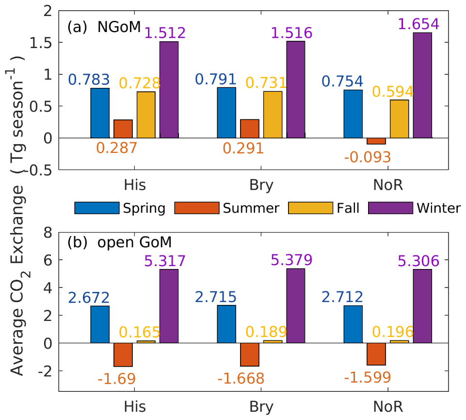
Figure 13 Seasonal air–sea CO₂ exchange at NGoM and the open GoM region among the His (historical), Bry (fixed boundary), and NoR (non-river) experiments.

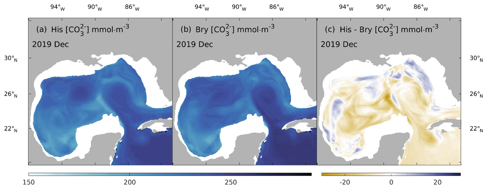
Figure 14 Comparison of monthly averaged carbonate ion concentration ([CO${}_{\mathrm{3}}^{\mathrm{2}-}$]) between His and Bry at 100 m depth in 2019. (a) December mean [CO${}_{\mathrm{3}}^{\mathrm{2}-}$] of the His experiment, (b) December mean [CO${}_{\mathrm{3}}^{\mathrm{2}-}$] of the Bry experiment, and (c) difference between (a) and (b).

The nondimensional model skill defined in Eq. (10) can be used to quantify the improvement of the model to reproduce observed data with regard to the climatological value:

$$\begin{array}{}\text{(11)}& \mathrm{skill}=\mathrm{1}-{\displaystyle \frac{{\sum }_{i=\mathrm{1}}^N{\left(d_i-I\left[m_i\right]\right)}^{\mathrm{2}}}{{\sum }_{i=\mathrm{1}}^N{\left(d_i-c_i\right)}^{\mathrm{2}}}},\end{array}$$

where d_i represents the available measurements, (d_i−ℑ[m_i]) is the observation–model difference, and (d_i−c_i) is the observation–climatology difference (Zhang et al., 2012). Usually, a skill of 0.25 means the model can reproduce 25 % more variance than those already described in climatology. By using the observation–model difference from this work and the observation–climatology difference from other models and climatology, we can evaluate the relative performance between this work as well as other models and climatology – a positive skill value ideally indicates improvement of the model in the numerator over the model and climatology in the denominator, while a negative skill value indicates the opposite. We use the other products as the reference to calculate the observation–product difference in the denominator, use our model to calculate the observation–model difference in the numerator, and list the corresponding skill value in Table 2, indicating the percentage improvement or deterioration gained by this work over the referenced product.

In Fig. 15, we interpolate regional model results to the nearest location of the underway surface pCO₂ measurements. We limited the observational data from 1 January 2001 to 31 December 2014 to ensure the ideal coverage of most products. Model results by Xue et al. (2016) only had temporal coverage from 2005 to 2010. Surface DIC, TA, temperature, and salinity from Gomez et al. (2020) were downloaded from NCEI Accession 0242495 (Gomez et al., 2021) to derive the surface pCO₂ patterns according to the method described in their paper. Underway pCO₂ observation data are compared with model results of the nearest year in Fig. 15. The statistics of model–data comparison are listed in Table 2.

For regional models, the 12-month ML-based climatology product by Chen et al. (2019) has the best performance in terms of RMSE (35.67) and skill (−0.11) (Table 2). However, the 12-monthly climatology product suffers from a temporal disadvantage when compared with model products with smaller time frequency. For example, model Chen 2019 had an R value of 0.54, while the daily averaged model (this work) had an R value of 0.59. The multiyear monthly product by Xue et al. (2016) has the largest RMSE (84.92) among the tested products and overestimates shelf regions while underestimating pCO₂ in the open-ocean region (especially the Loop Current). Overall, model Xue 2016 performs poorly in regard to surface pCO₂ with a low R value of 0.20 and a low TSS of 0.24, and the model in this study can reproduce 80 % more variance than that already described in model Xue 2016 (the skill of this work over model Xue 2016 is 0.80). In addition, the TSS of this work is 0.63, which is higher than that of the model Xue 2016 (0.24), supporting one of the major findings of this work that the NGoM is a carbon sink instead of a source during summer. Likewise, the open ocean should not be as strong a carbon sink as Xue et al. (2016) suggested since their estimated pCO₂ in the open ocean is significantly lower than the observations. Model results by Gomez et al. (2020) had a relatively low RMSE of 42.65 and a relatively high TSS of 0.57 among all models. When using model Gomez 2020 as the reference, this work generated a skill score of 0.22. Figure 15 reveals that model Gomez 2020 tends to overestimate pCO₂ on the northwest shelf of the GoM and underestimate it in the open ocean, especially the southern GoM connected with the Caribbean seas.

In Fig. 16, we extracted the monthly surface pCO₂ trend at two buoy locations from the regional models and climatology products to be compared with the monthly averaged buoy pCO₂ measurements. Taylor diagrams are shown for an integrated evaluation of the standard deviation and correlation coefficient of each model and climatology product concerning observation at the two buoy locations. At the two buoy locations, most products tend to overestimate the summer pCO₂, with model Xue 2016 yielding the largest overestimation. The coastal buoys recorded a typical low during the May, June, and July period, but most products failed to capture such a trend. Global models with coarse resolution and simplified, if any, river flux prescriptions generally perform poorly in the coastal region. Even for the relatively well-performing regional Gomez 2020 and the ML-based model Chen 2019, an overestimation as large as 100 µatm during May or June is found. Such an overestimation likely results in a reduced air–sea CO₂ flux when the ocean is a carbon sink (for flux estimates see Table 3). As shown in Fig. 16, this work can capture the monthly climatology of surface pCO₂ at two buoy locations relatively well. Such agreements result in relatively better correlation coefficients (with smaller p values) and standard deviation within the range of [25 50] for CoastalMS and [50 75] for CoastalLA in Fig16. Both the monthly time series and the Taylor diagrams in Fig. 16 reveal the benefits of this regional model as a good description of the coastal carbon system under the influence of the MARS.

Table 2 Statistics of surface pCO₂ comparison.

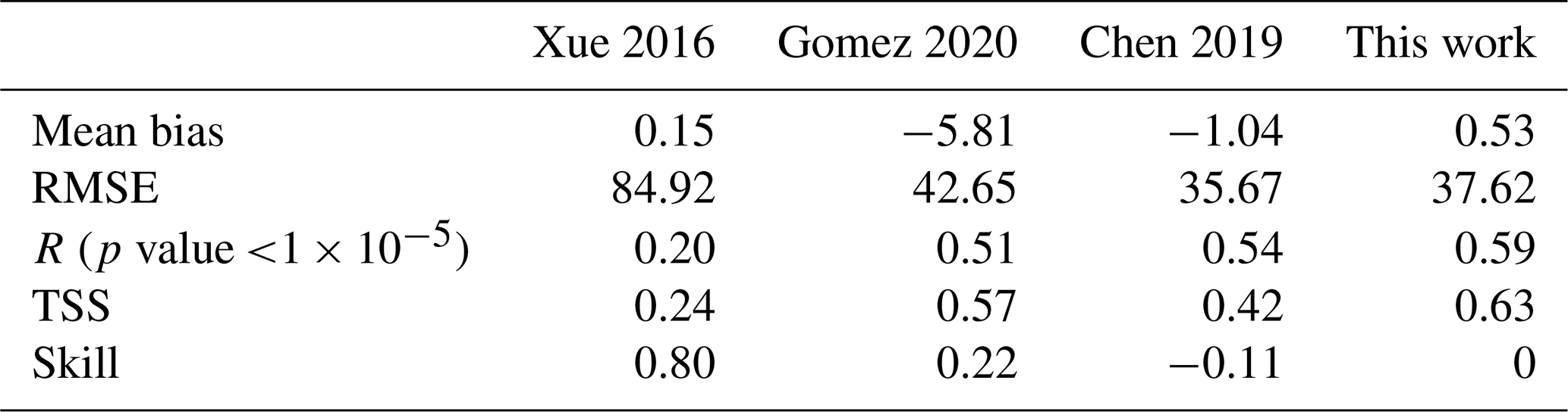
Figure 15 Comparison of sea surface pCO₂ between regional ocean model products (Xue 2016, Gomez 2020, Chen 2019, this work) and underway sea surface pCO₂ measurements. A positive ΔpCO₂ indicates that the product data overestimate sea surface pCO₂. A negative ΔpCO₂ suggests that the product data underestimate sea surface pCO₂. A neutral ΔpCO₂ indicates that the product data agree well with the observed sea surface pCO₂. The white spaces between the cruise lines indicate that these regions do not have observational pCO₂ data and do not indicate neutral bias.

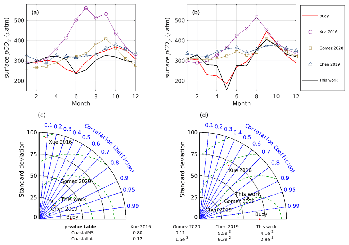
Figure 16 Comparison of sea surface pCO₂ among regional ocean model products (Xue 2016, Gomez 2020, Chen 2019, this work) at two buoy sites. Climatology at the two buoy locations of Gomez et al. (2020) is calculated by multiyear averaging from 2000–2014 model surface results. Climatology at the two buoy locations of Xue et al. (2016) is calculated by multiyear averaging from 2005–2010. Climatology at the two buoy locations of Chen et al. (2019) is calculated from their 12-monthly ML surface pCO₂ product (from July 2002 to December 2017). Buoy raw observations have a frequency of ∼ 3 h, and monthly averages are used to be compared with monthly model estimates. The p value for each correlation coefficient is listed in the p-value table.

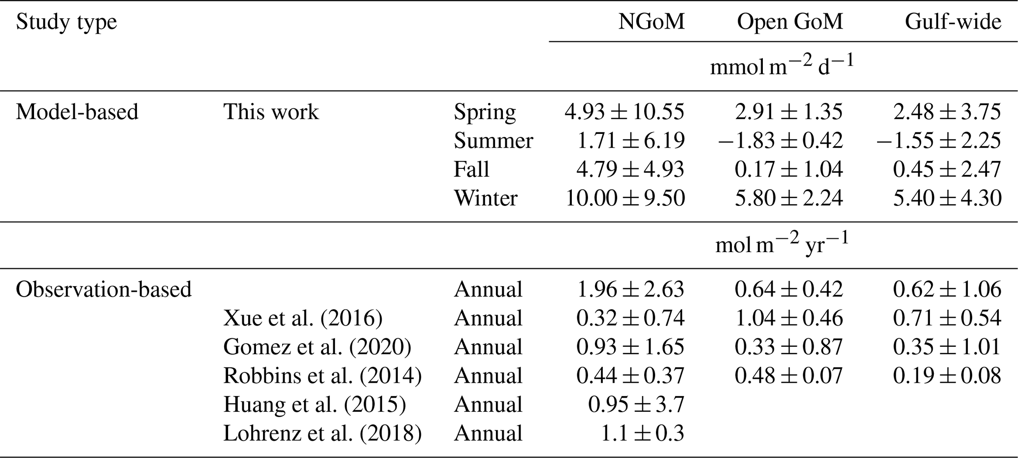
Table 3 Air–sea CO₂ flux comparison among this work and previous studies for the GoM. The mean estimate is followed by the standard deviation with the ± symbol. Positive flux indicates the ocean is a carbon sink with regard to the atmosphere.

5.2 Air–sea flux

In Table 3, we compare the annual air–sea CO₂ flux generated by this work with that reported by Xue et al. (2016) for 2005–2010, Gomez et al. (2020) for 2005–2014, Robbins et al. (2014) for 1996–2012, Huang et al. (2015) for 2004–2008, and Lohrenz et al. (2018) for 2006–2010. Using the same gas transfer velocity parameterization as this study, Xue et al. (2016) simulated a smaller carbon sink in the NGoM and a larger carbon sink estimation in the open GoM due to their overestimation of shelf pCO₂ and underestimation of the open GoM pCO₂, as shown in Fig. 15. The large bias of the open GoM carbon sink by Xue et al. (2016) likely results from the oversimplified prescription of the initial and boundary condition of DIC and TA (based on the empirical relationship with temperature and salinity), which led to an overestimation of carbon sink in the open GoM (1.6 times the value reported by this work and up to 3 times that reported by Gomez et al., 2020). To compare with the flux estimates of Gomez et al. (2020), we rescaled our estimates to the gas transfer velocity parameterization used in their work (based on Wanninkhof, 2014) and produced mean estimations of 1.59 ± 2.13, 0.52 ± 0.34, and 0.50 ± 0.86 mol m⁻² yr⁻¹ for the NGoM, open GoM, and gulf-wide, respectively. It is expected that this work estimated a larger carbon sink in the NGoM region compared with that of Xue et al. (2016) and Gomez et al. (2020), as revealed in Figs. 15a–b and 16a–b. Surface pCO₂ in the coastal region simulated by Xue et al. (2016) is significantly overestimated, as shown in Figs. 15 and 16a–b. This model bias corresponds to the smallest NGoM carbon sink estimation in Table 3. Similarly, surface pCO₂ in the coastal NGoM region and at the two buoy locations was overestimated by Gomez et al. (2020) (Figs. 15b, 16a, b). This pCO₂ overestimation can be a reason for its smaller carbon sink estimation for the NGoM compared with that of Lohrenz et al. (2018), Huang et al. (2015), and this work. Additionally, the NGoM is a carbon source from June to October according to Gomez et al. (2020), which is different from what we simulated in this study (NGoM is a carbon sink all year-round). Combining information from Fig. 16, where Gomez et al. (2020) overestimate pCO₂ by ∼ 50 µatm on average during June at the two coastal locations, we conclude that the NGoM air–sea CO₂ sink by Gomez et al. (2020) is likely underestimated. The observation-based studies by Huang et al. (2015) yielded an annual sink of 0.96 ± 3.7 mol C m⁻² yr⁻¹ for NGoM based on wind data from the monthly satellite product QuikSCAT (12.5 km resolution). Lohrenz et al. (2018) estimated an annual sink of 1.1 ± 0.3 mol C m⁻² yr⁻¹ for NGoM using gas transfer velocities estimated for each 8 d period. To sum up, we conclude that the air–sea CO₂ flux generated by this work is more robust in the NGoM region than that in previous model and climatology products. Nevertheless, a direct carbon flux comparison between model and observation-based studies needs to account for the differences in wind data and the gas transfer velocities.

5.3 Outlook and future model development

A likely warmer climate combined with heavier precipitation and greater river discharge is predicted in the following years for the MARS (Dai et al., 2020; Fischer and Knutti, 2015; Frei et al., 1998; Tao et al., 2014), although climate change might reduce precipitation for some low- and middle-latitude regions (Arora and Boer, 2001; Na et al., 2020). A warmer climate will reduce the momentum of the Loop Current, and less tropical water (reduced by about 20 %–25 %) will be introduced into the GoM from the Caribbean (Liu et al., 2012). As a consequence, the Loop Current might penetrate less into the NGoM and reduce the upwelling along the NGoM and WF slope. Stronger river discharge with nutrient loads will exacerbate the NGoM acidification in bottom water (Laurent et al., 2018) while increasing the surface water biological CO₂ utilization and removal, creating larger river plume regions that exhibit a distinct carbon footprint compared to surrounding waters. Such predictions resemble the perturbation prescribed in the Bry and NoR experiments, wherein a reduced global ocean impact can be assessed by the difference between Bry and His experiments, and impacts from increased river discharge can be assessed by the difference between His and NoR experiments. We anticipate the open GoM to be a stronger carbon sink in the future under the projection of Loop Current weakening. And the NGoM will continue to be a strong carbon sink, with the sink region expanded in response to predicted greater river discharge and smaller momentum in the Loop Current.

Field samples of the carbon system give us synoptic knowledge of the carbon cycle in the ocean. However, carbon system attributes are subject to large fluctuation due to temperature, salinity, mixing, and biological activities; current observations of the carbon system at the sea surface or vertically along transects are far from enough to reveal the carbon system evolution in the GoM. As ship-based observations are limited by spatial coverage and temporal coverage, mooring observations have a high frequency (∼ 3 h) in time but only cover limited geological locations. The ML model derived from remote sensing and cruise data inherits the bias from satellite ocean color products and ship-based measurements, and, more importantly, it assumes that the training data contains all information that defines the system it is trying to predict, which is not necessarily the truth. One benefit of numerical models is to offer information to bridge fragmentary knowledge and fill in the gaps between observations and reality. However, the marine carbon cycle is admittedly a complex process. Several simplifications and parameterizations are needed to perform a numerical simulation. Nevertheless, specifications for some key processes may warrant further investigation and better parameterization. (1) The multiple alkalinity generation processes in the sediment pool (Fennel et al., 2008; Thomas et al., 2009) in current experiments are linked linearly with the aerobic decomposition of PON with a fixed ratio, which can potentially induce large bias during high PON concentrations. The anoxic zone chemistry component can be added to properly simulate the carbonate system in oxygen-deficient conditions (Raven et al., 2021), which can prevail in bottom boundary layer waters in coastal regions in NGoM, especially during summer. Adding in anoxic zone chemistry will also allow a more diversified prescription for TA generation, which plays a key role in the understanding of sediment pH dynamics (Gustafsson et al., 2019; Middelburg et al., 2020). (2) In our model, the density-related fragmentation or flocculation of detritus OM is simplified with one particulate and one dissolved pool, each with a fixed sinking rate. Coagulation and flocculation can transform DOC into particulate OM or subsequently form large aggregates, whose remineralization rate can be much faster (Ploug et al., 1999). The remineralization–sinking dynamic determines the fate of OM decomposition (and water column DIC profile) and should be allowed to have more degrees of freedom in future model development. (3) Calcification in this work can reflect the primary factors regulating marine calcification. However, important feedback from water acidity on the calcification is omitted due to the overall supersaturation with aragonite in GoM shelf waters. Therefore, the modeled CaCO₃ $/$ PON ratio could not reflect the decreasing trends of the CaCO₃ $/$ PON ratio under acidification (Zondervan et al., 2001). (4) Phytoplankton groups can play different roles in carbon cycling given their different sizes, sinking rates, and calcification rates, among others, and their relative ratio would be critical to the carbon dynamic (Le Moigne et al., 2015; Poulton et al., 2007). The interplay between zooplankton grazing and phytoplankton bloom in this work captured the seasonal dynamic but only had fixed modes toward nutrient levels. High nutrient concentration favors the success of diatoms, and a lower nutrient level gives small phytoplankton a competitive advantage in NGoM (Aké-Castillo and Vázquez, 2008; Chakraborty and Lohrenz, 2015; Qian et al., 2003; Strom and Strom, 1996). More phytoplankton groups and possible predation avoidance mechanisms could be added to the model to give the bloom pattern (and subsequently the carbon export) more variance (Liszka, 2018; Rost and Riebesell, 2004). (5) Adding the higher-trophic-level biology could be the next step to improving the model. Marine fishes are reported to produce precipitated carbonates within their intestines at high rates and contribute to TA increase in the top 1000 m of ocean waters (Wilson et al., 2009). (6) This model did not include sediment silicate weathering and carbon flux through atmospheric deposition, which can potentially be important sources and sinks of carbon to the ocean waters as well (Jurado et al., 2008; Wallmann et al., 2008).

6 Conclusions

This study presents a high-resolution regional carbon model for the GoM with fully coupled carbonate chemistry calculations and air–sea interaction. The model can reliably simulate the spatial and temporal pattern of the surface ocean carbon system. We show, for the first time, a solid validation of a regional carbon model via direct comparison against high-frequency CO₂ buoys, TA $/$ DIC vertical profiles along the coastal transects, a remote-sensing-based ML model product, and underway pCO₂ measurements (surface). We calculated the decadal trends of important carbon system variables such as pCO₂, pH, air–sea CO₂ exchange, and Ω over the NGoM and open GoM regions.

The GoM surface pCO₂ values experience a steady increase from 2001 to 2019, with an increasing rate of 1.61 µatm yr⁻¹ in NGoM and 1.66 µatm yr⁻¹ in the open GoM, respectively. Correspondingly, the ocean surface pH is declining at a rate of 0.0020 and 0.0015 yr⁻¹ for NGoM and open GoM, respectively. The surface Ω over the NGoM and open GoM region remains supersaturated with aragonite during the time span of the model but with a slightly decreasing trend. The carbon sink of both NGoM and open GoM regions exhibits increasing trends and will continue to increase at a faster pace in the coming years under the prospect of climate change with rising atmospheric pCO₂.

We decouple the influence on surface pCO₂ into thermal and nonthermal components and further analyze the surface pCO₂ changes due to gross primary production and air–sea CO₂ flux. We find that the low temperature during winter and the biological uptake during spring and summer are the primary drivers making GoM an overall CO₂ sink. During the modeled period of 2001–2009, the GoM overall is a CO₂ sink with a mean flux rate of 0.62 mol C m⁻² yr⁻¹ (11.77 Tg C yr⁻¹). The NGoM region is a CO₂ sink year-round and is very susceptible to changes in river forcing. The open GoM region is dominated by thermal effects and converts from a carbon sink to a source during summer.

The historical simulation (His) and perturbed tests (Bry, NoR) are performed to determine whether observed changes in the GoM carbon system are driven by secondary effects of carbon accumulation from the global ocean or local forcing, such as river inputs. The results show that, in addition to the increasing atmospheric pCO₂ over the GoM, the spatial distribution and trend in carbon system variables could only be explained when the effects of carbon accumulation via boundary conditions and the impact from river discharge are included. Although eliminating carbon accumulation via boundary in the Bry experiment did not bring a significant difference in surface carbon variables compared with that of His, a clear chemical equilibrium shift between [CO${}_{\mathrm{3}}^{\mathrm{2}-}$] and [HCO${}_{\mathrm{3}}^{-}$] can be observed at subsurface depths under the perturbation of the accumulative boundary carbon concentrations. With a projected warming climate, we anticipate the GoM to be a stronger carbon sink due to elevated river discharge and reduced impact from the global ocean.

Appendix A

Table A1 Summary of CMIP6 GCMs considered for boundaries conditions of the regional model.

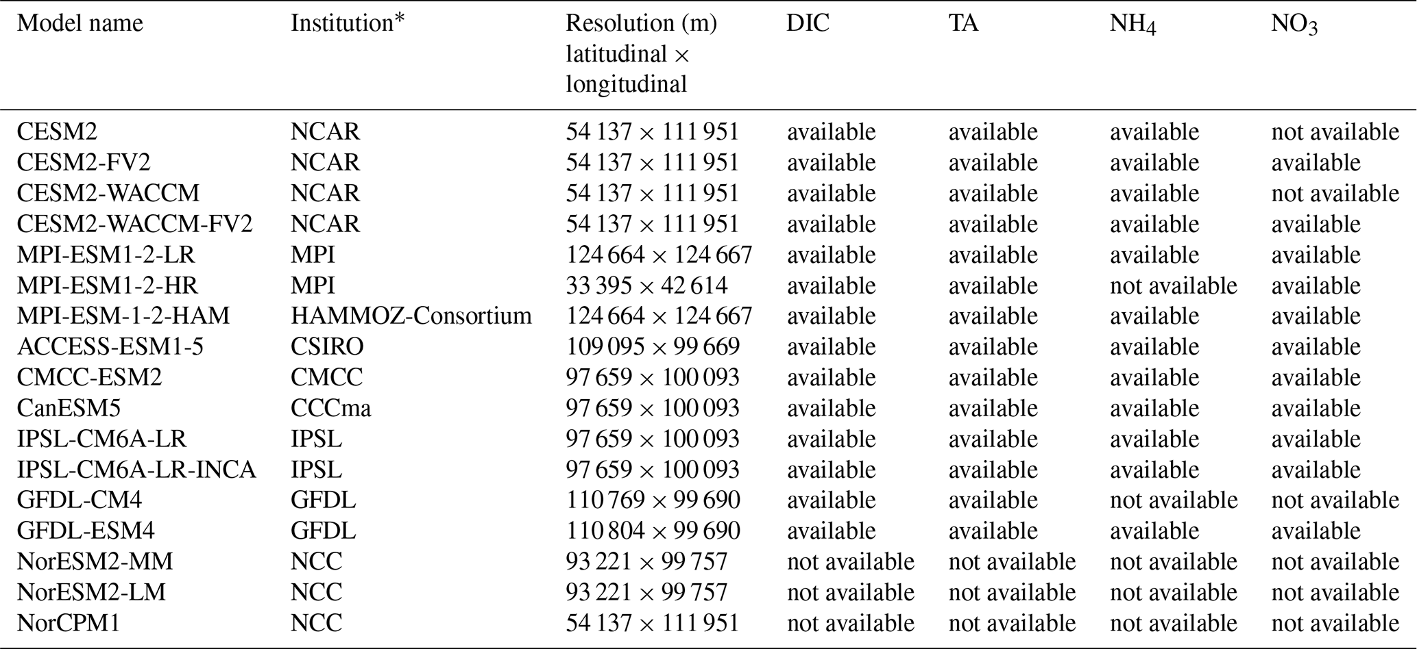
^* Full names of institutions are as follows. CCCma: Canadian Centre for Climate Modelling and Analysis (Canada). CSIRO: Commonwealth Scientific and Industrial Research Organization and Bureau of Meteorology (Australia). CMCC: Centro Euro-Mediterraneo per I Cambiamenti Climatici (Italy). IPSL: L'Institut Pierre-Simon Laplace (France). MPI: Max Planck Institute for Meteorology (Germany). NCC: Norwegian Climate Centre (Norway). NCAR: National Center for Atmospheric Research (US). GFDL: Geophysical Fluid Dynamics Laboratory (US).

Table A2 Model boundary frequency.